the Creative Commons Attribution 4.0 License.
the Creative Commons Attribution 4.0 License.
 | 28 Jan 2022
Thirty-eight years of CO2 fertilization has outpaced growing aridity to drive greening of Australian woody ecosystems
Sami W. Rifai
Martin G. De Kauwe
Anna M. Ukkola
Lucas A. Cernusak
Patrick Meir
Belinda E. Medlyn
Andy J. Pitman
Climate change is projected to increase the imbalance between the supply (precipitation) and atmospheric demand for water (i.e., increased potential evapotranspiration), stressing plants in water-limited environments. Plants may be able to offset increasing aridity because rising CO2 increases water use efficiency. CO2 fertilization has also been cited as one of the drivers of the widespread “greening” phenomenon. However, attributing the size of this CO2 fertilization effect is complicated, due in part to a lack of long-term vegetation monitoring and interannual- to decadal-scale climate variability. In this study we asked the question of how much CO2 has contributed towards greening. We focused our analysis on a broad aridity gradient spanning eastern Australia's woody ecosystems. Next we analyzed 38 years of satellite remote sensing estimates of vegetation greenness (normalized difference vegetation index, NDVI) to examine the role of CO2 in ameliorating climate change impacts. Multiple statistical techniques were applied to separate the CO2-attributable effects on greening from the changes in water supply and atmospheric aridity. Widespread vegetation greening occurred despite a warming climate, increases in vapor pressure deficit, and repeated record-breaking droughts and heat waves. Between 1982–2019 we found that NDVI increased (median 11.3 %) across 90.5 % of the woody regions. After masking disturbance effects (e.g., fire), we statistically estimated an 11.7 % increase in NDVI attributable to CO2, broadly consistent with a hypothesized theoretical expectation of an 8.6 % increase in water use efficiency due to rising CO2. In contrast to reports of a weakening CO2 fertilization effect, we found no consistent temporal change in the CO2 effect. We conclude rising CO2 has mitigated the effects of increasing aridity, repeated record-breaking droughts, and record-breaking heat waves in eastern Australia. However, we were unable to determine whether trees or grasses were the primary beneficiary of the CO2-induced change in water use efficiency, which has implications for projecting future ecosystem resilience. A more complete understanding of how CO2-induced changes in water use efficiency affect trees and non-tree vegetation is needed.
- Article
(15560 KB) - Full-text XML
- BibTeX
- EndNote


Australia is the world's driest inhabited continent. Predicting how climate change will affect ecosystem resilience and alter Australia's terrestrial hydrological cycle is of paramount importance. Australia's woody ecosystems are mostly concentrated in the east, where there are large gradients of precipitation (P) (300–2000+ mm yr−1) and potential evapotranspiration (PET) (800–2100 mm yr−1). Most eastern Australian woodlands occupy water-limited regions where annual PET far exceeds P (Fig. A1 in the Appendix), and tree species have evolved to cope with water-limited conditions (Peters et al., 2021) and high interannual rainfall variability. However, the climate is warming: 8 of Australia's 10 warmest years on record have occurred since 2005 (CSIRO and Bureau of Meteorology, 2020), and Australia's climate has warmed by ∼ 1.5 ∘C since records began in 1910. The warming has likely increased atmospheric demand for water (e.g., PET or vapor pressure deficit, VPD). In most woody ecosystems, the ratio of water supply (i.e., P) to water demand (i.e., PET) has declined in recent decades (Figs. 1, 2a). Eastern Australia has also been impacted by several multi-year droughts, episodic deluges of rainfall (King et al., 2020), and an increasing frequency of severe heat waves (Perkins et al., 2012) in the last few decades. Precipitation changes have been spatially variable over eastern Australia, where northern Queensland grew wetter, and southeastern Australia grew drier (Fig. 2a). In the last 2 decades, southeastern Australia experienced the two worst droughts in the observational record (2001–2009; van Dijk et al., 2013; and 2017–2019; Bureau of Meteorology, 2019). Yet between these two droughts, eastern Australia experienced record-breaking rainfall in 2011 associated with a strong La Niña event. This caused marked vegetation “greening” (e.g., increased foliar cover), even in the arid interior (Bastos et al., 2013; Poulter et al., 2014; Ahlstrom et al., 2015). However, this greening contributed to record-breaking fires in the following year (Harris et al., 2018).
Theory suggests that plant physiological responses to atmospheric carbon dioxide (CO2) may mitigate some of the negative effects of an aridifying climate. However, the magnitude of plant responses to increased atmospheric CO2 has been challenging to establish in field experiments (Jiang et al., 2020b) and from observations (Frankenberg et al., 2021; Zhu et al., 2021; Walker et al., 2020) or to separate from other drivers (e.g., climate variability, disturbances, and changes in land management; Zhu et al., 2016). Studies have used data from the Advanced Very High Resolution Radiometer (AVHRR) satellites to show positive trends in the normalized difference vegetation index (NDVI) over Australia (Donohue et al., 2009). The greening trend is caused by increased leaf area, which has likely resulted from increased atmospheric CO2 concentrations (Donohue et al., 2013; Ukkola et al., 2016). The evidence for increases in leaf area from rising CO2 has also been supported by observations of reduced runoff in Australia's drainage basins (Trancoso et al., 2017; Ukkola et al., 2016).
Yet disentangling the CO2 fertilization effect from other drivers of climate variability and global change has been particularly challenging for satellite-based analyses. It is challenging to attribute causes of greening because co-occurring changes in climate, land use, and disturbance are confounded by the effect of CO2 fertilization. Furthermore, the time series of even the longest systematically collected optical vegetation index records from a single sensor is 20 years (e.g., MODIS Terra). Analysis of trends extending beyond 20 years requires merging satellite records across sensors and platforms. But this requires care to address changes in radiometric and spatial resolution of the sensor as well as drift in the solar zenith angle (Ji and Brown, 2017; Frankenberg et al., 2021) and the time of retrieval. Thus different analytical methodologies have produced disagreements over where greening has occurred (Cortés et al., 2021). One often-used method to provide additional constraint on greening trends has been to compare remote-sensing-derived trends with modeled changes in leaf area index (LAI) from ensembles of dynamic global models (Zhu et al., 2016; Wang et al., 2020). However these model attribution approaches rely on a set of key assumptions. None of the models can accurately predict LAI changes in response to rising CO2 (De Kauwe et al., 2014; Medlyn et al., 2016). Vegetation models have been shown to diverge in their simulation of LAI over Australia (Medlyn et al., 2016; Teckentrup et al., 2021; Zhu et al., 2016) and have bioclimatic rules for determining phenology which may not be appropriate for the highly variable Australian climate and the evergreen Eucalyptus forests (Teckentrup et al., 2021). These model simulations are typically compared with modeled LAI products derived from the red and near-infrared wavelengths of multispectral satellite sensors, of which each product carries specific algorithmic assumptions about canopy-light interception which are conditional upon estimated land cover types. In comparison, NDVI carries no ecosystem-specific assumption and is an effective proxy for leaf area in ecosystems with low to moderate canopy cover (Carlson and Ripley, 1997), a characteristic of eastern Australian woody ecosystems (Specht, 1972; Yang et al., 2018).
Here we ask how much greening trends can be explained by rising CO2. Using eastern Australia as a model system, we used a multi-satellite-derived NDVI record encompassing 38 years with multiple statistical techniques to isolate the influence of CO2 from simultaneous effects of meteorological change and disturbance. Next we contrasted CO2 effects with theoretical predictions based on water use efficiency (WUE) theory for plants and the observed rise in CO2. Finally, we examined whether recent NDVI greening trends have co-occurred with changes in tree or grass cover over the last 2 decades.
2.1 Study area
The study region encompasses the dominant woody ecosystems of eastern Australia (Fig. A1b). We used the National Vegetation Information System 5.1 land cover dataset (Australian Department of Agriculture, Water and the Environment, 2020; Table A1) to select locations designated as “Acacia Forests and Woodlands”, “Acacia Open Woodlands”, “Callitris Forests and Woodlands”, “Casuarina Forests and Woodlands”, “Eucalypt Low Open Forests”, “Eucalypt Open Forests”, “Eucalypt Open Woodlands”, “Eucalypt Tall Open Forests”, “Eucalypt Woodlands”, “Low Closed Forests and Tall Closed Shrublands”, “Mallee Open Woodlands and Sparse Mallee Shrublands”, “Mallee Woodlands and Shrublands”, “Melaleuca Forests and Woodlands”, “Other Forests and Woodlands”, “Other Open Woodlands”, “Rainforests and Vine Thickets”, and “Tropical Eucalypt Woodlands/Grasslands”.
2.2 Climate and remote sensing datasets
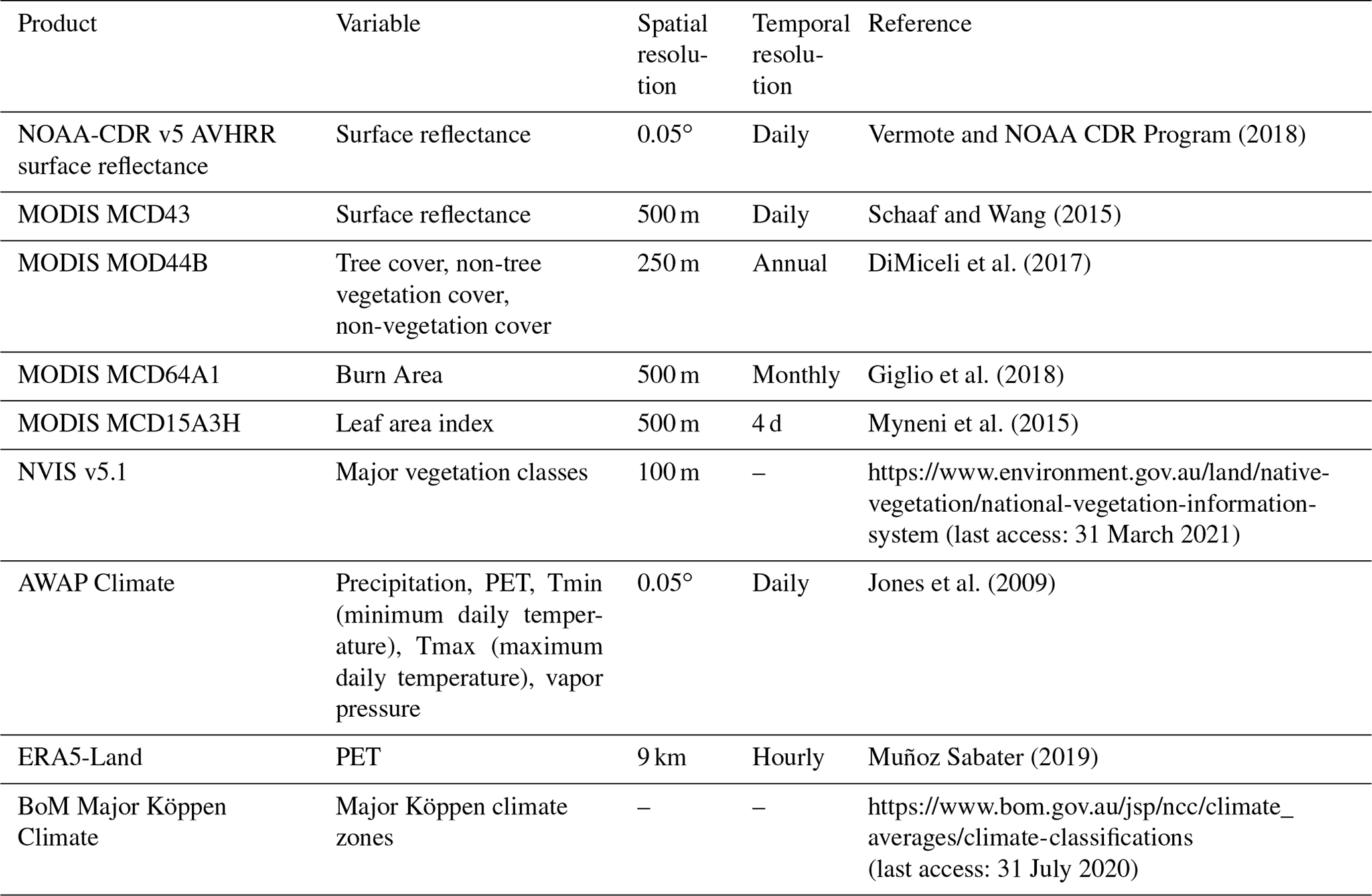
We used the atmospheric CO2 record from the deseasonalized Mauna Loa record (https://www.esrl.noaa.gov/gmd/ccgg/trends/data.html, last access: 5 April 2020) and extracted climate data (Table A1) from the Australian Bureau of Meteorology's Australian Water Availability Project (AWAP; Jones et al., 2009). AWAP is a gridded climate product interpolated to 0.05∘ from a large network of meteorological stations distributed across Australia. Vapor pressure deficit was calculated using daily estimates of maximum temperature and vapor pressure at 15:00 LT (UTC+10). PET was calculated from shortwave radiation and mean air temperature using the Priestley–Taylor method (Davis et al., 2017). The Priestley–Taylor method has been shown to be appropriate for estimating large-scale PET (Raupach, 2000) and is more suited for use in long-term analysis where CO2 has increased than other common formulations such as the Penman–Monteith equation (Greve et al., 2019; Milly and Dunne, 2016), which explicitly imposes a fixed stomatal resistance that is incompatible with plant physiology theory (Medlyn et al., 2001). AWAP measurements of shortwave radiation only extend back to 1990, so we extended the PET record to 1982 by calibrating the ERA5-Land PET record (1980–2019) to the AWAP PET record (1990–2019) by linear regression for each grid cell and then gap-filled the years 1982–1989 with the calibrated ERA5 PET. PET from the Climate Research Unit record (Harris et al., 2014) was highly correlated with both the recalibrated ERA5 PET (r=0.91, 1982–1989) and the original AWAP PET (r=0.97, 1990–2019). Next, we calculated a 30-year climatology of the meteorological variables using the period of 1982–2011 to be close to current standards (World Meteorological Organization, 2017). We used this climatology to define the mean annual P : PET (the moisture index, MIMA) and as the reference to calculate a 12-month running anomaly of annual P : PET (MIanom). Zonal statistics for each meteorological variable were calculated using simplified Köppen climate zones, derived from the Australian Bureau of Meteorology (Fig. 2b, Table A1).
We used surface reflectance from two satellite products to generate the NDVI record: National Oceanic and Atmospheric Administration's Climate Data Record v5 Advanced Very High Radiometric Resolution (AVHRR) Surface Reflectance (NOAA-CDR) and the National Aeronautics and Space Administration's MCD43A4 Nadir Bidirectional Reflectance Distribution Function Adjusted Reflectance (MODIS-MCD43) (Table A1; Schaaf and Wang, 2015). NDVI data were extracted from 1982–2019 at 0.05∘ resolution from the NOAA-CDR AVHRR version 5 product (Vermote and NOAA CDR Program, 2018). The surface reflectance record of AVHRR extends through 2019, but the quality of the record starts to degrade in 2017 because of an increase in the solar zenith angle (Ji and Brown, 2017), causing a sensor-produced decline in NDVI during 2017–2019. For this reason we only use AVHRR surface reflectance data between 1982–2016. We composited monthly mean AVHRR NDVI (NDVIAVHRR) estimates using only daily pixel retrievals with no detected cloud cover (quality assurance band, bit 1). Monthly NDVIAVHRR estimates aggregated from fewer than three daily retrievals were removed. They were also removed when the coefficient of variation in daily retrievals for a given month was greater than 25 %. We also removed NDVIAVHRR monthly estimates where NDVIAVHRR, solar zenith angle, or time of acquisition deviated beyond 3.5 standard deviations from the monthly mean, calculated from a climatology spanning 1982–2016.
We used the MODIS-MCD43 surface reflectance at 500 m resolution to derive NDVI for 2001–2019 (NDVIMODIS). Monthly mean estimates of the surface reflectance were produced by compositing pixels flagged as “ideal quality” (quality assurance, bits 0–1). We also masked disturbances to have greater confidence in our attribution of the targeted drivers of NDVIMODIS change (climate and CO2). The Global Forest Change product v1.7 (Hansen et al., 2013) was used to mask pixels from 2001 onwards that had experienced forest loss due to deforestation or severe stand clearing disturbance. We masked pixel locations that experienced bushfires from the year 2001 onwards. Specifically, these pixels were masked for the year of burning and the following 3 years using the 500 m resolution MODIS-MCD64 monthly burned-area product (Giglio et al., 2018). We terminated the NDVIMODIS time series in August of 2019, prior to the widespread bushfires of late 2019/early 2020. Both NDVIAVHRR and NDVIMODIS datasets were processed using Google Earth Engine (Gorelick et al., 2017) and exported at 5 km spatial resolution, which best approximated the native resolution of the NOAA-CDR AVHRR and AWAP products. Further post-processing used the “stars” (Pebesma, 2020) and “data.table” (Dowle and Srinivasan, 2019) R packages (see “Code and data availability” section).
We merged the processed 1982–2016 NDVIAVHRR with the 2001–2019 NDVIMODIS by recalibrating the NDVIAVHRR with a generalized additive model (GAM). Specifically, we used 1 million observations from the overlapping 2001–2016 portion of both records to fit a GAM using the “mgcv” R package (Wood, 2017) to model NDVIMODIS from AVHRR-derived covariates as
where “s” represents a penalized smoothing function using a thin plate regression spline; SZA is the solar zenith angle; NDVIAVHRR is the uncalibrated NDVI from AVHRR; TOD is time of day of retrieval; and x and y represent longitude and latitude, respectively. The fit GAM was then used to generate the recalibrated AVHRR NDVI. The merged NDVI dataset was created by joining the 1982–2000 recalibrated AVHRR NDVI with the 2001–2019 NDVIMODIS. We further reduced monthly temporal variability in NDVI by calculating a 3-month rolling mean of NDVI, which we used for subsequent statistical model fitting.
2.3 Estimating NDVI and climate trends
We estimated the relative increase in NDVI between 1982–2019 with respect to time (Eq. 2) for each grid cell with an iteratively weighted least squares robust linear model via the “rlm” function in R's MASS package (Venables and Ripley, 2002) as follows.
Here β0 represents the estimated NDVI in 1982, the year term starts at 1982, and the sensor term is a binary covariate that accounts for residual offset differences between the recalibrated AVHRR NDVI and the NDVIMODIS. The relative temporal trends for climate variables and the MODIS vegetation continuous fractions were fit for each grid cell location using the Theil–Sen estimator, a form of robust pairwise regression, with the “zyp” R package (Bronaugh and Werner, 2019). The temporal covariate was recentered to start with the first hydrological year (where the year starts 1 month earlier in December) of the data so that the intercept term represents the mean at the start of the time series. The relative rate of change for each variable was reconstructed by calculating
where β0 and β1 are the intercept and trend derived from Theil–Sen regression.
2.4 Estimating contribution of CO2 and climate toward NDVI trends
We fit six forms of statistical models to the merged NDVI observations in order to quantify the impact of changes in CO2 and meteorological variables on NDVI. Figure 1 shows that the relationship between NDVI and multi-annual mean of P : PET was nonlinear and followed a monotonic saturating sigmoidal relationship. GAMs can characterize a nonlinear response without specifying a functional form, yet the underlying spline parameters are not easily interpreted as the parameters of a fixed nonlinear function. Therefore we fit models with a set of fixed nonlinear functional forms using nonlinear least squares (nls.multstart package in R v4.01; Padfield and Matheson, 2020) and compared models fit using all pixel locations. The nonlinear functional forms included the Weibull function (Eq. 4, Fig. 5), the logistic function (Eq. 5, Fig. A5), and the Richards growth function (Eq. 6 Fig. A6). We focused on the Weibull models because they showed equivalent goodness of fit with fewer parameters than the Richards function models. Next we added a linear modifier to the Weibull function using the covariates of CO2 (µmol µmol−1; Ca) and the ratio of the anomaly of P : PET (MIanom) to the mean annual P : PET (MIMA) as follows:
Here the sensor term is a binary covariate indicating the AVHRR or MODIS sensor. Model-fitted parameters Va and Vd correspond to the asymptote and the asymptote's difference from the minimum NDVI, while cln is the logarithm of the rate constant, and q is the power to which MIMA is raised. The model was fit by individual season with 1 million observations per model fit. Corresponding goodness-of-fit metrics (R2 and root mean square error) were calculated by season (Fig. 5) with 1 million randomly sampled observations.
We tested alternative nonlinear functional forms to characterize the effect of CO2 upon NDVI. A logistic model was fit across space for each hydrological year as
where NDVI is the hydrological year mean value of NDVI for a grid cell location, m is the midpoint, s is a scale parameter, and VA is the asymptote (plotted in Fig. A5). We also used a modified Richards growth function to characterize the CO2 effect upon seasonal NDVI (Fig. A6) as
Here the β terms act to linearly modify the core nonlinear parameters (VA, m, s, q) with the effects of CO2 and MIf.anom. Each seasonal model component was fit across space with 1 million random samples from the total merged NDVI record (approximately 14.3 million observations).
To ensure consistent interpretation of the nonlinear response across P : PET, we also fit linear models explaining NDVI with CO2 and MIanom by season in MIMA bin widths of 0.2 (Eq. 7, Fig. A4). Separate linear models were fit for increments of 0.15 of MIMA for each season using the merged 1982–2019 NDVI record. NDVI was modeled as
where Veg. Class is the NVIS 5.1 vegetation class, and sensor is a binary variable used to account for residual differences between the recalibrated AVHRR NDVI and NDVIMODIS records. To aid the comparison of model effects, we centered and standardized the continuous model covariates before regression. The standardized CO2 and P : PETanom effects (β) are presented in Fig. A4.
Next, to produce spatially varying estimates of the CO2 effect, we fit robust multiple linear regression models to the time series of NDVI for each of the 39 463 pixel locations. The CO2 effect for each grid cell location was simultaneously estimated with the linear effects of the anomalies (anom) of P, PET, VPD, and MI as fractions of their mean annual (MA) values as follows:
Finally we produced a GAM to estimate the CO2 effect in addition to the nonlinear interactions between CO2, mean annual climate, and climate anomalies. Here instead of predetermined nonlinear functional forms, the GAM used penalized smoothing functions (s) to estimate the potentially nonlinear effect of the covariates. The GAM was fit across all pixel locations and estimated the CO2 effect and the effects of the anomalies and mean annual values of VPD, P, and PET as well as sensor epoch as follows:
2.5 A simplified theoretical water use efficiency model
We compared the statistically attributed CO2 amplification of NDVI with the expectation from a simple theoretical model of WUE. Following Donohue et al. (2013), WUE (W) is defined as
where A is leaf-level carbon assimilation (µmol m2 s−1), E is leaf-level transpiration (µmol m2 s−1), Ca is atmospheric CO2 (µmol µmol−1), Ci is intercellular CO2 (µmol µmol−1), χ is , and D is atmospheric vapor pressure deficit (mol mol−1). The relative rate of change in W with respect to a change in Ca can be calculated as
If temperature increases without a corresponding increase in humidity, D increases, which also causes transpiration to rise and thus reduces W. However, W is predicted to increase with CO2, which may offset increases in D. Experiments suggest that χ does not change with Ca but is sensitive to D (Wong et al., 1985; Drake et al., 1997) and can be estimated as being proportional to the square root of D (Medlyn et al., 2011). By substituting into Eq. (11) we can estimate the theoretical combined effect of Ca and D upon Wleaf as
Transpiration per unit ground area is strongly controlled by water supply in warm, water-limited environments with relatively low leaf area such as eastern Australia (Specht, 1972); therefore we approximate canopy transpiration (Ecanopy) as
where L is leaf area. The change in Ecanopy can then be defined as
If we assume there is no overall change in precipitation then we can assume change in Ecanopy is tightly coupled to the water supply; therefore we have
We note that the assumption of constant precipitation is obviously unrealistic, most notably because two major droughts occurred during the observation period. However, over much longer periods (i.e., 1910–2018) precipitation in eastern Australia has been relatively stationary (Ukkola et al., 2019).
NDVI is linearly related to foliar cover (F) until LAI ≈ 3 (m2 m−2) (Carlson and Ripley, 1997), which is predominantly the case when P : PET < 1. Most woody ecosystems in eastern Australia are strongly water-limited with LAI ≤ 1 (m2 m−2), where NDVI is approximately proportional to the fraction of foliar cover:
Then substituting Eq. (15) into Eq. (12) gives
If we assume that the benefit towards Wleaf from rising Ca is split evenly between the relative changes in Aleaf and F, we can predict the change towards NDVI to be
We compared the WUE theoretical model with the robust linear models fit for each pixel location (Eq. 8) and the GAM (Eq. 9) fit across the study region. The WUE theoretical model assumes no change in P but does account for changes in VPD. Therefore in using the statistical models to compare with the WUE predictions, we generated counterfactual predictions from the statistical models with no precipitation anomaly but with the observed increases in CO2 and VPD. One weakness with the application of this WUE theoretical model is the uncertainty regarding the assumed allocation of the Wleaf benefit towards either Aleaf or F (e.g., LAI; see above). Donohue et al. (2017) proposed a similar model to Eq. (18), the partitioning of equilibrium transpiration and assimilation (PETA) hypothesis, where the relative allocation to leaf area is predicted to decline with increasing resource availability (which could be inferred from growing season LAI). We calculated the expectation from the PETA hypothesis as another point of comparison with the CO2-attributable effect on NDVI.

Figure 1Individual grid cell temporal 38-year trajectories of the normalized difference vegetation index (NDVI) and the ratio of annual precipitation (P) to potential evapotranspiration (PET). A vector field plot showing the direction of change in mean annual NDVI and P : PET between 1982–1986 and 2015–2019 for 1000 randomly sampled grid cell locations (color indicates direction of change in P : PET as indicated by legend). An inset shows a magnification of the samples from the 0.1–0.4 P : PET range. The distributions of mean P : PET (mm mm−1) and NDVI for the period of 1982–1986 are shown as histograms above and to the right of the main panel. Note that the majority of arrows shift towards higher aridity (lower P : PET) and higher NDVI.
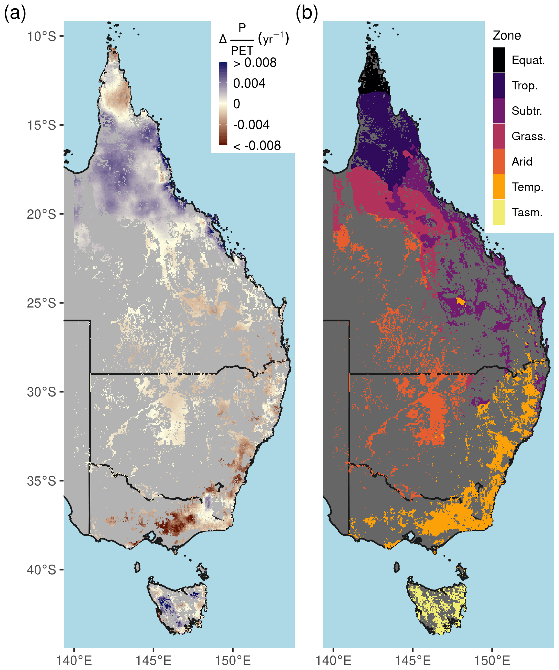
Figure 2Long-term aridity change and climate zones. (a) The linear trend of annual P : PET (the moisture index) between 1982–2019, (b) simplified Köppen climate zones. Climate zone abbreviations correspond to Equatorial (Equat.), Tropical (Trop.), Subtropical (Subtr.), Grassland (Grass.), Temperate (Temp.), and Temperate Tasmania (Tasm.).
3.1 Long-term greening in a changing climate
Parts of northern Queensland grew wetter, but aridity (as measured by reduced P : PET) increased in over 52 % of eastern Australian woody ecosystems since 1982 (Figs. 1, 2a). Aridity decreased over northern Queensland, encompassing the entirety of Equatorial and Tropical regions and most of the Grassland and Subtropical regions, driven by large wet-season increases in precipitation (Fig. A2a). Widespread increases in PET were evident from September–February (Fig. A2b). At the same time as these changes in climate were occurring, over 92 % of these regions experienced overall greening (Fig. 3a), including regions where P : PET declined (Figs. 1, 2b, A3). The relative increases in NDVI were comparable between the earlier AVHRR epoch (1982–2000) and the later MODIS epoch (2001–2019) at 5.7 % (CI = [−2.9 %, +20.3 %]) and 5.1 % (CI = [−6.4 %, +20.1 %]), respectively. However, the spatial patterns of greening and/or browning differed between epochs (Fig. 3b), and most regions also showed high decadal-scale variability in greening and/or browning trends (Fig. 4). The overall greening trends between the AVHRR 1982–2000 epoch and the MODIS 2001–2019 epoch generally agree across regions and seasons. However linear NDVI trends fit over shorter intervals of 10 years are much less consistent (Fig. 4), exemplifying the importance of estimating trends over long enough periods to average over decadal-scale variability. Long-term browning only occurred in the Arid region (Figs. 3, 4). Nevertheless, by examining NDVI trends over nearly 40 years, we were able to separate regional decadal-scale variability from the overall broad greening trend across eastern Australia (Figs. 3, 4, A3).
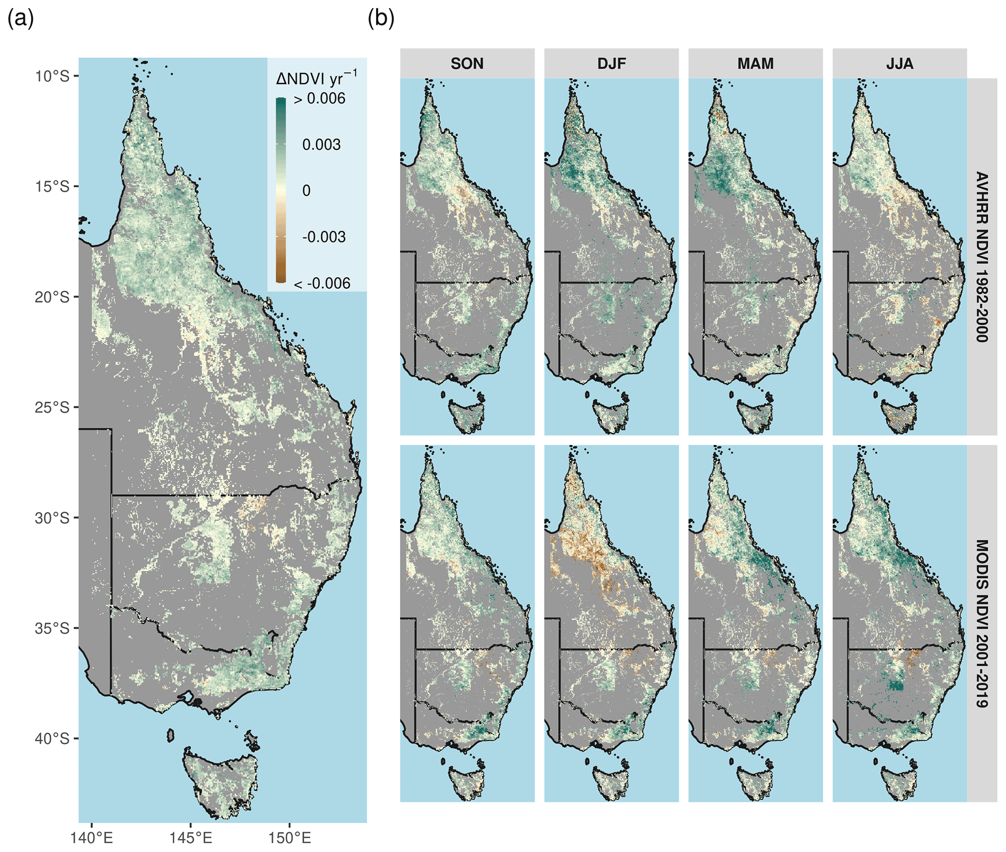
Figure 3Overall long-term NDVI change and change shown by satellite epoch and season. (a) The annual rate of NDVI change from the merged satellite record spanning 1982–2019. The seasonal AVHRR NDVI between 1982–2000 (b, top row) and MODIS NDVI between 2001–2019 (b, bottom row). Non-woody ecosystem regions are masked in gray. A notable browning trend is evident at the interface of the Grassland and Arid regions during DJF of the MODIS time period. Note: season abbreviations correspond to September–October (SON), December–February (DJF), March–May (MAM), and July–August (JJA).
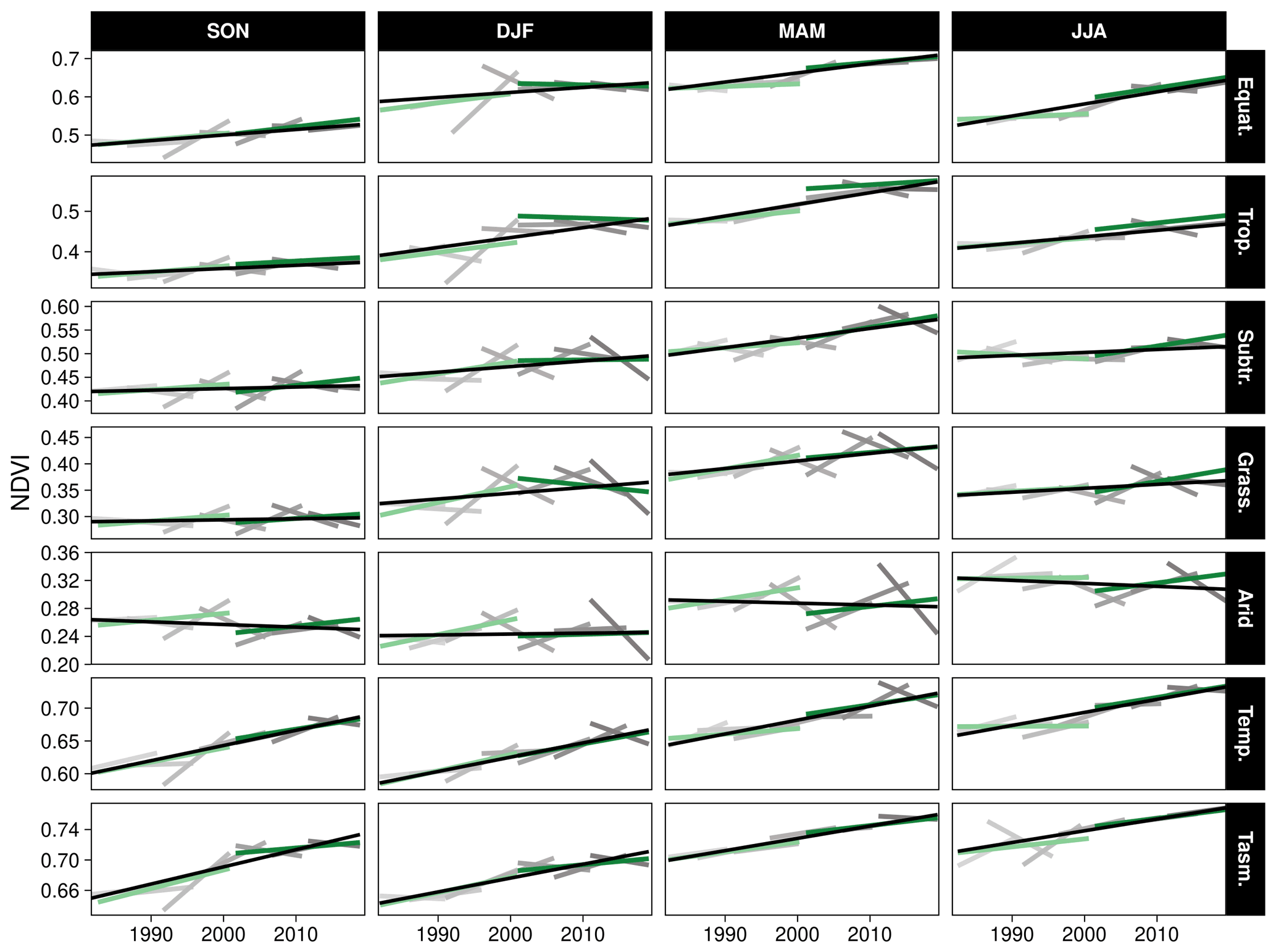
Figure 4Variability in linear trends over varying time periods by season and climate zone. The black line represents the overall 1982–2019 trend, the light-green line represents the calibrated 1982–2000 AVHRR, and the green line represents the 2001–2019 MODIS. Gray colors indicate linear trends from overlapping 10-year time intervals. The boundaries of the climate zones are shown in Fig. 2b. Note: climate zone abbreviations correspond to Equatorial (Equat.), Tropical (Trop.), Subtropical (Subtr.), Grassland (Grass.), Temperate (Temp.), and Temperate Tasmania (Tasm.). Season abbreviations correspond to September–October (SON), December–February (DJF), March–May (MAM), and July–August (JJA).
3.2 Empirical attribution of the CO2 effect
We found consistently positive NDVI responses to CO2 across the moisture gradient of P : PET for all seasons, with the greatest increases located in regions of higher P : PET (>0.5) (Fig. 5). The nonlinear Weibull models showed a larger CO2-attributable effect on NDVI in regions of higher P : PET (Fig. 5), but the effect size of the NDVI response to CO2 was largely consistent across model forms (Figs. A4–A7). The CO2-attributable increase in NDVI between 1982–2019 ranged from approximately 5 % in the Arid interior regions to >20 % in the wettest Tropical and Temperate regions (Fig. 5a). This was consistent with linear model forms when fit for individual grid cell locations (Eq. 8, Fig. 6) as well as by comparing the CO2 effect size across 16 linear models fit for grid cell locations grouped into bins spanning 0.1 increments of P : PET (Eq. 7, Fig. A4). The GAM fit across grid cell locations also indicated a larger CO2 effect in regions with higher P : PET (Figs. 6, 7b). Quantile regression with generalized additive models showed a pronounced response to CO2 across the distribution of pixels with both low and high NDVI (10–97.5 percentiles) across the full aridity gradient of P : PET (Fig. A7).
A recent study found that the global CO2 fertilization effect was halved between the 1980s and 2000s (Wang et al., 2020). In contrast to the estimates over eastern Australia from Wang et al. (2020), we found no consistent evidence of a decline in the effect of CO2 on NDVI through time. Neither the GAM estimates nor the robust linear model estimates of the CO2 effect showed any consistent evidence of a weakening CO2 effect between 1982–2000 and 2001–2019 (Fig. 6). The central 25th–75th percentiles of the distribution of robust linear model effect sizes overlapped in all regions between epochs. The central 25th–75th percentiles of the GAM-estimated distributions also overlapped, with the exception of the Grassland and Arid regions, where the CO2 effect was larger during 2001–2019. Consistent with the finding of a greater CO2 effect in wetter regions (Fig. 5), the robust linear models and the GAM estimated the CO2 effect to be greatest in the Equatorial and Tropical regions and lowest in the Arid region (Fig. 6).
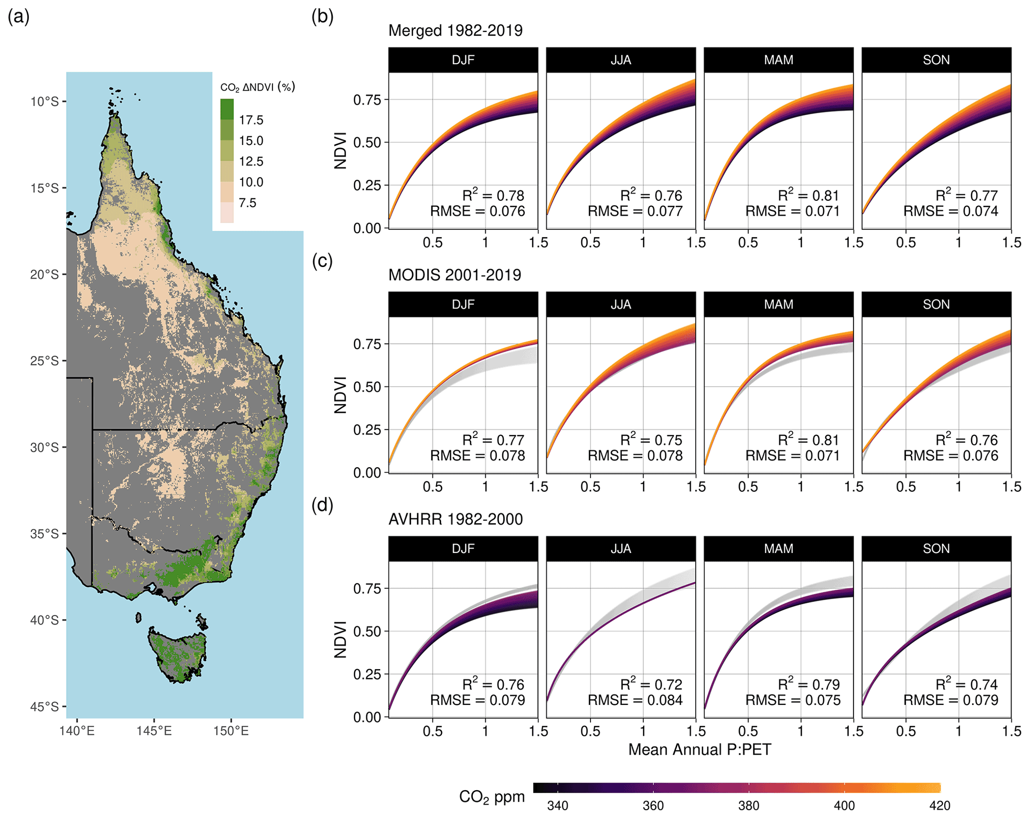
Figure 5Effect of increasing CO2 on seasonal NDVI across P : PET. Predictions of seasonal NDVI as a function of mean annual P : PET fit using a standard Weibull function (see “Methods”, Eq. 2), modified with linear effects of CO2, the running 12-month anomaly of P : PET, and the satellite sensor. The CO2 concentration gradient represents the atmospheric CO2 change between 1982–2019. Panel (a) maps the total predicted contribution of CO2 towards the relative increase in NDVI between 1982–2019 assuming no anomaly of P : PET. Panel (b) shows the merged sensor response between 1982–2019 across the gradient of mean annual P : PET, (c) shows the model response when fit using just MODIS MCD43 data between 2001–2019, and (d) shows the response when the model was fit with the recalibrated AVHRR data between 1982–2000. The AVHRR- and MODIS-satellite-epoch NDVI predictions are plotted in gray for (b) and (c), respectively.
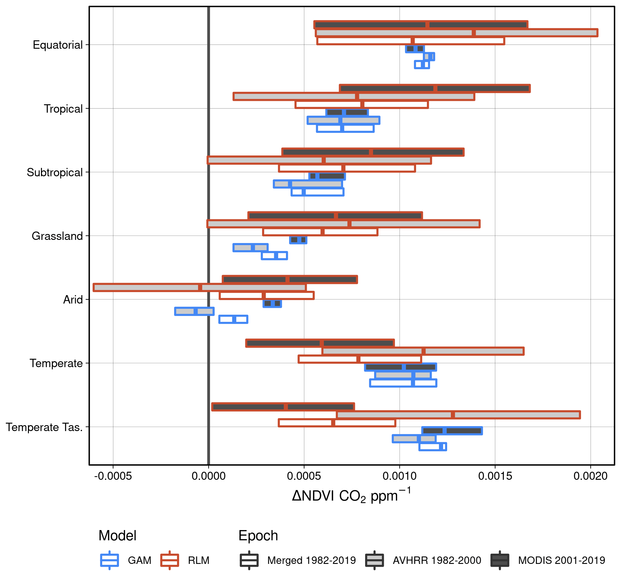
Figure 6Boxplot representation of the CO2-attributable effect upon changing NDVI. Here the 25th, 50th, and 75th percentiles of the CO2-attributable effect on NDVI are shown. The robust linear models (RLM; see “Methods”, Eq. 13) were fit for each individual grid cell location, whereas the generalized additive model (GAM; see “Methods”, Eq. 14) was fit using all grid cell locations. The distribution of RLMs yielded a median R2 of 0.58 and RMSE of 0.025 over the merged period. The GAM had an overall R2 of 0.91 and RMSE of 0.049.
3.3 CO2-driven greening and expectations from water use efficiency
The range of statistically estimated CO2-attributable greening responses were compared with the expectation from the theoretical CO2 water use efficiency model. The Donohue et al. (2013) CO2×WUE model (see “Methods”) accounts for changes in VPD but assumes no change in water supply. Assuming an equal split in the benefits of WUE between greater carbon assimilation and increased foliage cover (see below for alternative assumptions), the model predicted an 8.7 % (10th–90th percentile range [+6.8 %, +10.2 %]) increase in NDVI (proxy for foliage cover; see “Methods”). This compared to an estimated 11.7 % ([+4.6 %, +14.6 %]) relative increase from the GAM when accounting for a simultaneous increase in VPD (which the WUE accounts for) and factoring out the effects of changing precipitation and PET (which the WUE model does not account for). We needed to assume differing levels of allocation to foliar gain (i.e., not 50 %) for the theoretical WUE model to match the statistically estimated CO2 effect (Fig. 7e). Regions of higher P : PET (Equatorial, Tropical, Temperate, and Temperate Tasmanian) required greater allocation fractions than 50 %, whereas the allocation fraction would be between 25 %–50 % for regions with lower P : PET (Arid, Grassland, and Subtropical). In comparison, the PETA hypothesis (Donohue et al., 2017) predicted the greatest CO2 effect on leaf area to be in regions with the lowest LAI, but this was not supported by the statistically estimated CO2 effect on NDVI (Fig. A9). Despite having the lowest LAI, the Arid region received the smallest CO2 effect, but it is worth noting that the Arid region also experienced the greatest increase in VPD and reduction in P over the 38-year period (Figs. 7a, A8). In contrast, the largest estimated CO2-attributable effects on greening were found to be in the Equatorial and Tropical areas.
3.4 Co-occurring shifts in aridity, NDVI, and vegetation cover
The shifts in P : PET and NDVI were accompanied by vegetation cover changes in some regions. Most notably, the Arid and Temperate regions experienced the strongest zonally averaged declines in P : PET (Fig. 8a) and increases in VPD (Fig. A8). Seasonal greening trends were relatively similar apart from the aforementioned exceptions in the Grassland. The MODIS vegetation continuous fraction data from 2001–2018 indicated that most regions experienced modest changes in tree vegetation cover. The largest decline in tree cover occurred in the Temperate regions (Figs. 8c, A10). Most regions experienced declines in non-vegetated (bare) cover, increases in non-tree vegetation, and modest change in tree cover (Fig. 8c); however the proportional increase in non-tree vegetation typically exceeded tree cover increases (Fig. A10).
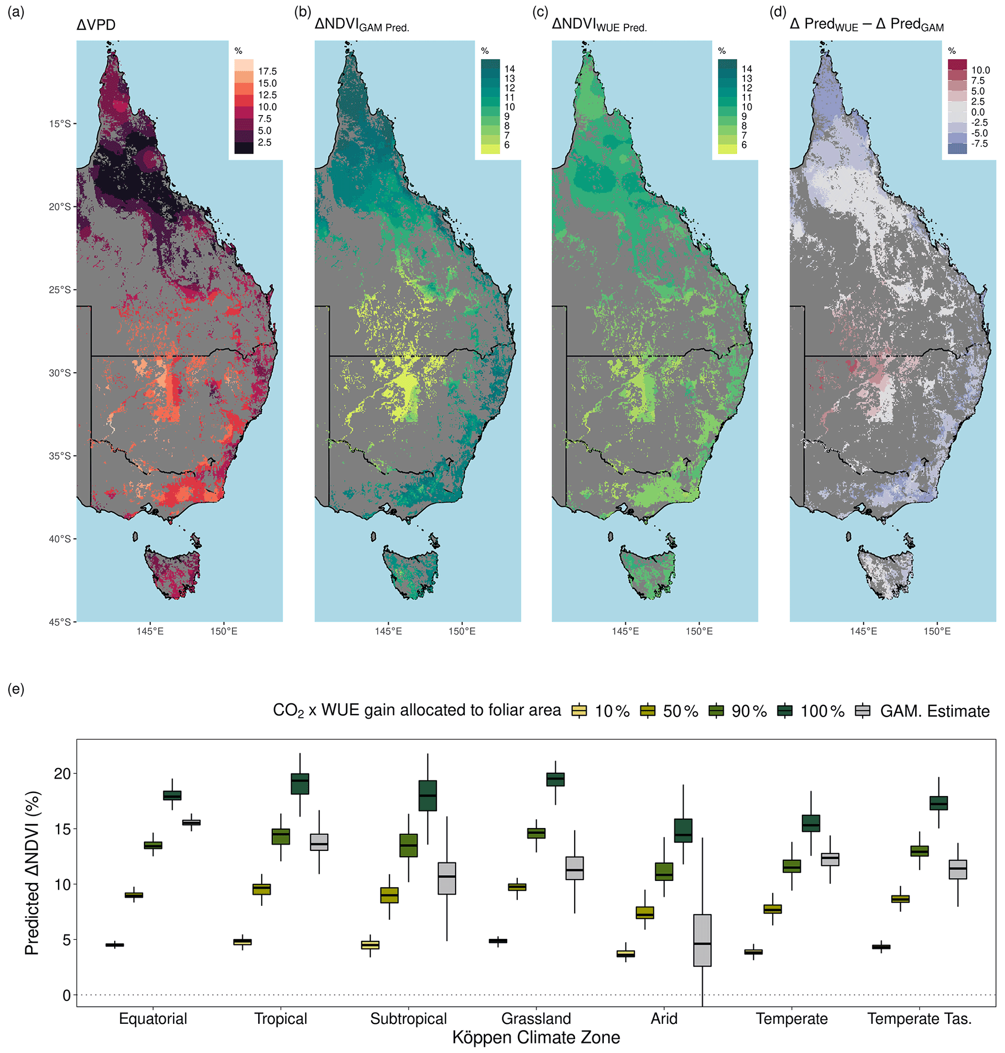
Figure 7Long-term changes in vapor pressure deficit and comparison between the ΔNDVI due to CO2 and the expected CO2 fertilization effect on foliar area due to gains in water use efficiency (WUE). (a) The relative increase in the annual mean of vapor pressure deficit (VPD) between 1982–2019. (b) The predicted relative increase in NDVI due to CO2 (see “Methods”, Eq. 14) with a concurrent increase in VPD. (c) The relative expected increase in NDVI following the theoretical WUE prediction where 50 % of the gain is allocated to foliar area (see “Methods”, Eq. 11). (d) The difference between the predictions of relative NDVI from the WUE model with 50 % allocation and the GAM-estimated relative increase caused by CO2. Blue regions indicate where the GAM prediction was greater than the WUE prediction. (e) Boxplot of the expected relative NDVI % increase from WUE gains due to CO2 fertilization depending upon differing levels of foliar allocation from the CO2 benefit toward WUE and the GAM-estimated NDVI% increase due to CO2 (see “Methods”, Eq. 11). The boxplot distribution of the Equatorial region appears collapsed because the Equatorial portion of the region is relatively small (a).
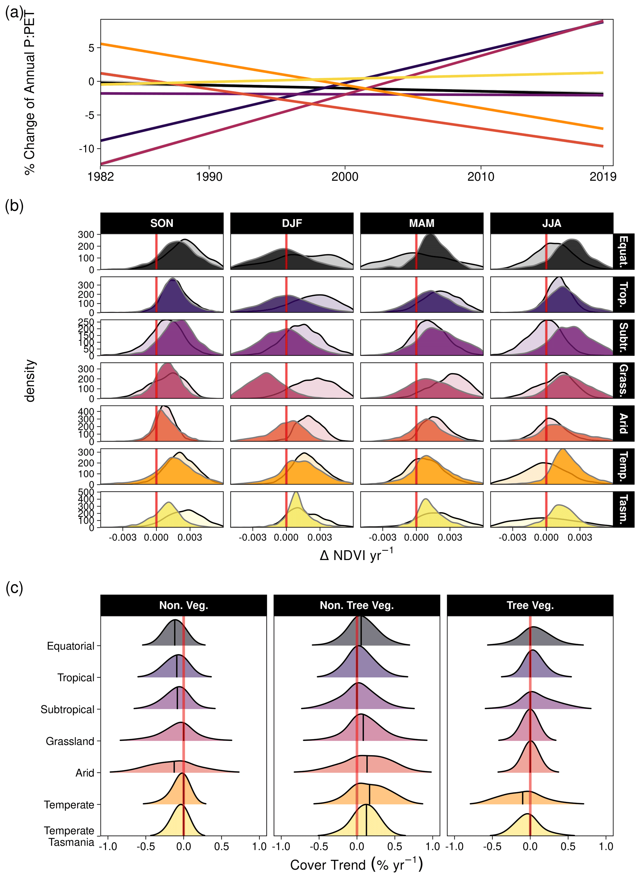
Figure 8The relative percentage change in P : PET by climate zone and corresponding distributions of ΔNDVI yr−1 and percentage annual change in vegetation cover fraction. (a) The linear relative changes in annual P : PET trend by climate zone between 1982–2019, as estimated by robust regression (see “Methods”). The annual P : PET change (%) and corresponding standard error were as follows: Equatorial (−0.045 ± 0.01), Tropical (0.477 ± 0.005), Subtropical (−0.007 ± 0.005), Grassland (0.576 ± 0.006), Arid (−0.293 ± 0.006), Temperate (−0.342 ± 0.004), and Temperate Tasmania (0.047 ± 0.005). (b) Distribution of linear long-term NDVI trends for the six climate clusters by season using the Theil–Sen estimator. Filled distributions are trends from the MODIS sensors (2001–2019), and transparent (black outline) distributions are from the AVHRR sensors (1982–2000). (c) Distributions of the linear pixel-level trends using the Theil–Sen estimator for non-vegetated cover, non-tree vegetation cover, and tree cover between 2000–2018. The median is overlaid. Note that climate zone abbreviations are as follows: Equatorial (Equat.), Tropical (Trop.), Subtropical (Subtr.), Grassland (Grass.), Temperate (Temp.), and Temperate Tasmania (Tasm.).
4.1 Australian woody vegetation as model systems to quantify CO2 fertilization
Australia is ideal to explore the CO2 contribution towards vegetation greening because there are fewer confounding effects to drive greening. Forest trees are evergreen, and the growing season is rarely limited by temperature or radiation. The study region spans a large moisture gradient (Fig. A1a), but unlike much of the global tropics, the large majority of the study region is not so cloudy as to prevent multiple high-quality multispectral satellite retrievals per month. Australia has also not been subjected to other prominent drivers of greening such as nitrogen deposition (Ackerman et al., 2019). Nevertheless, Australia has experienced notable land use change during the study period such as high rates of deforestation in Queensland and northern New South Wales (Evans, 2016). However, we excluded affected pixel locations from the analysis.
Prior global analyses on warm arid environments have quantified the CO2 effect on greening (Donohue et al., 2013). More expansive global-scale analyses of all terrestrial vegetation using dynamic global vegetation model attribution have found evidence to connect Australia's greening to changes in atmospheric CO2 concentration (Winkler et al., 2021), while an earlier study did not (Zhu et al., 2016). Australian studies documented the greening trend up to 2010 using the long-term AVHRR record (Donohue et al., 2009; Ukkola et al., 2016) and have been able to partially attribute CO2 as a driver of greening in sub-humid and semi-arid regions. Here we advanced upon prior research to separate the effects of disturbance and changes in aridity and moisture in order to quantify the CO2 fertilization effect across the full spectrum of moisture availability experienced by Australian woody ecosystems, notably for 38 years.
4.2 Regional differences in greening and browning through time
Despite the region's high decadal-scale variability in NDVI (Fig. 4), the nearly 4-decade-long record allowed us to separate the CO2 effect on NDVI from the anomalies caused by drought (e.g., 2003–2009) or high rainfall (e.g., La Niña 2010–2011). Although the long-term greening trends we document in the 9 years following earlier studies are generally consistent (Donohue et al., 2009; Ukkola et al., 2016), our results diverge and lead to key differences in interpretation of why NDVI has continued to increase. First, while the relative increases in NDVI between the 1982–2000 AVHRR epoch (5.7 %) and the 2001–2019 MODIS epoch (5.1 %) are comparable (Figs. 3b, 8b), the underlying reasons for the change differ. VPD changed minimally between 1982–2000, whereas it rapidly increased between 2001–2019 (Fig. A8). These increases were largest in the most Arid and Temperate regions (12.7 % and 11 % since 1982, respectively; Fig. 6), and when coupled with seasonal reductions in precipitation (Fig. A2) these would have partially offset benefits from increased intrinsic water use efficiency (Eq. 17). In contrast, more than half of the Equatorial, Tropical, Subtropical, and Grassland regions in northern Queensland experienced increases in precipitation since 1982 (Fig. A2; Ukkola et al., 2019), thus allowing these locations to exceed the predicted NDVI increases from the WUE model (Fig. 7d).
It should be noted that not all regions experienced consistent greening trends throughout the observation period. For example, “greening” shifted to “browning” during the austral summer (December–February) in the Arid and Grassland regions of Queensland between the 1982–2000 and 2001–2019 records (Fig. 3b). It is unclear why browning occurred during austral summertime in the Grassland region (Figs. 3b, 4, 8b). The declines in NDVI during 2001–2019 may have been meteorologically driven and related to shifts in the distribution of wet- and dry-season precipitation (Fig. A2). Alternatively, the shift could be due to changes in fire and cattle management that have been particularly prevalent across regions of Queensland in recent decades (Seabrook et al., 2006). Further, greening may have been suppressed in parts of Queensland because cattle ranching activity has intensified and has driven forest conversion to managed pasture in the region (McAlpine et al., 2009).
4.3 Attributing a CO2 fertilization contribution towards greening
Plants increase their rates of photosynthesis in response to rising atmospheric CO2 whilst also reducing stomatal conductance, which reduces evaporative losses, and combined, the two responses lead to greater WUE (Ainsworth and Rogers, 2007; Morison, 1985). In water-limited ecosystems, it has been hypothesized that this physiological response by plants to CO2 should result in increased leaf biomass (Donohue et al., 2013; Ukkola et al., 2016). While all of our statistical approaches indicated a year-round positive CO2 effect, in contrast to theory the effect was consistently greater in regions with higher P : PET (Figs. 5–7, A4–A7). Our analysis also diverges with a global coarse-scale analysis that found weakening of the CO2 fertilization effect across both southeastern and northern Australia (Wang et al., 2020). We found no meaningful difference in the CO2-attributable effect towards greening between the AVHRR 1982–2000 and MODIS 2001–2019 epochs to support the finding of a temporally weakening CO2 effect (Fig. 6). The WUE model predicted similar relative rates of NDVI increase between the two epochs (4.5 % and 4.7 % for AVHRR and MODIS), yet for different reasons. CO2 increased by 30 ppm between 1982–2000, while VPD changed minimally, and precipitation increased in Queensland and the Arid region (Fig. A8), all of which are favorable to increasing NDVI. In contrast, the larger CO2 increase between 2001–2019 (40 ppm) was offset by a spatially ubiquitous increase in VPD (3.7 %, CI = [−0.4 %, 8.6 %]; Fig. A8) and the occurrence of two multi-year droughts (Millennium Drought, 2003–2009, and The Big Dry, 2017–2020). Despite the widespread evidence of the CO2 effect, the WUE model notably underpredicted greening in some regions (Fig. 7).
4.4 Deviations from WUE
We found that the CO2 effect on foliar area was the smallest in the driest climate regions (Figs. 5–6, A4–A7). This was at odds with the WUE prediction (at 50 % allocation; Fig. 7e) and contrary to the expectation that the greatest WUE-derived benefit from CO2 would be in drier climates (Donohue et al., 2017; McMurtrie et al., 2008). These deviations may have resulted from ecosystems processes beyond the scope of a simple model, such as more severe nutrient limitations, the phenology of the vegetation composition, belowground root processes, and disturbances not captured by the satellite products (e.g., small fires, grazing). Browning in the Grassland region (Figs. 3b, A3) may have been caused by distinct dry-season phenological differences between overstory woody vegetation and understory C4 grasses (Moore et al., 2016), which are dominant there (Murphy and Bowman, 2007). C4 grasses may have been favored over C3 because precipitation increased during the austral summer over the course of the study (Fig. A2), and this higher concentration of rainfall during the warmest months is thought to favor C4 grasses (Hattersley, 1983; Knapp et al., 2020; Murphy and Bowman, 2007). Finally, the linear dependency of leaf area upon VPD in the theoretical model may be ill-suited for extreme anomalously arid conditions because NDVI observations suggest a strongly nonlinear relationship with large VPD anomalies (Fig. A11).
We explored how much of the higher WUE benefit would have to be allocated to match the GAM-estimated CO2-attributed changes in NDVI. Allocation rates far greater than 50 % would be required to match the WUE prediction in the Tropical and Equatorial zones (Fig. 7e), whereas allocation would need to be less than 50 % to match the GAM estimate in the Arid region. The Arid region experienced the greatest relative increase in VPD (Figs. 7a, A8), yet the theoretical model still predicted a small but positive increase in NDVI (Fig. 7c), which the GAM estimate suggests would be closer to a 10 % rather than 50 % foliar allocation level from the WUE benefit (Fig. 7d). Nevertheless, the smaller effect over the Arid region was consistent with earlier observational findings across Australia (Ukkola et al., 2016) and experimentation from the Nevada Desert FACE experiment (Smith et al., 2014).
4.5 Relation to ecosystem CO2 fertilization experiments
Notably, a 4-year-long ecosystem-scale CO2 manipulation experiment carried out in a mature Eucalyptus woodland in Sydney (EucFACE) did not observe an increase in leaf area under elevated CO2 (Jiang et al., 2020b). The experimental site is located upon phosphorus poor soils, typical of Australia. The lack of a leaf area growth response observed at EucFACE is not necessarily inconsistent with the greening effect observed in this study. Our observational window of 38 years is much longer than the elevated CO2 exposure time in the experiment (4 years in Jiang et al., 2020b), covers different CO2 increments (historical vs. future), and could imply that woodlands are eventually able to liberate belowground phosphorus to support greater biomass growth on longer timescales. Increased autotrophic soil respiration and belowground productivity were observed at EucFACE under elevated CO2 exposure (Drake et al., 2016; Jiang et al., 2020b), as was a brief period of enhanced nitrogen and phosphorus mineralization (Hasegawa et al., 2016). Over time, this increased investment of carbon belowground could potentially liberate sufficient phosphorus to support an expansion of leaf area. The reduced allocation to foliar area in the Arid region (Fig. 7e) may reflect that extra carbon derived from CO2 is allocated belowground to increase water uptake or mitigate other resource limitations such as soil phosphorus (Jiang et al., 2020a).
4.6 Vegetation composition shifts
Most grid cell locations in the Temperate zone experienced simultaneous apparent declines in tree cover and increases in non-tree vegetation cover (e.g., grasses and shrubs) (Figs. 8c, A10). This is surprising because we focused this regression analysis on 2001–2018 in order to exclude the reduced tree cover due to the catastrophic megafires of 2019/20 (Nolan et al., 2020). Some may question the ability of the MODIS Vegetation Continuous Fraction product (DiMiceli et al., 2017) to accurately distinguish Australian tree cover from non-tree vegetation (Sexton et al., 2013; Adzhar et al., 2021); however this pattern is consistent with a recent lidar-derived tree cover time series of Australia (Liao et al., 2020). Future work may seek to uncover trends in the green vegetation fraction by analyzing higher-resolution data derived from the Landsat constellation, such as Geoscience Australia's vegetation fractional cover product (Gill et al., 2017). The decline in tree cover suggests that the drought starting in 2017 was already killing trees prior to the 2019/20 megafires. Field observations of tree decline remain relatively rare, but a citizen science initiative has documented more than 300 locations of non-fire-related mass tree mortality between 2018–2020 (Atlas of Living Australia, 2020). Similarly, a study using an experimental constrained plant hydraulics model to predict the regions at risk of drought-induced tree mortality found greater risk in the same arid regions of southeastern Australian forests and woodlands (De Kauwe et al., 2020). These predicted regions of mortality coincide with where we document the greening trends that fell short of the theoretical WUE expectation. These rapid shifts in vegetation underlie the need for greater continuous field vegetation monitoring to capture change imposed by climate extremes.
We separated the effects of disturbance and meteorological anomalies with statistical models to show that increasing CO2 produced nearly 4 decades of widespread vegetation greening across eastern Australia. The large agreement between a theoretical model and the statistically estimated CO2 effect indicated that greening resulted from an increase in water use efficiency. Vegetation greening occurred despite a highly variable and increasingly arid climate and on soils particularly poor in phosphorus, which have likely acted as a constraint on growth. While rising atmospheric CO2 ameliorated what would have been a browning woody ecosystem response to declining P : PET, the CO2 effect was insufficient to promote greening when both P and P : PET experienced long-term decline, as observed in the more arid regions in our study. Further, it is unknown whether further increases in atmospheric CO2 will continue to enable vegetation to mitigate increases in aridity and VPD under future warming. It is also unclear if trees or grasses are the primary contributors to the recent greening trend. Future localized work is urgently needed to better understand recent changes in tree and grass competition under an increasingly arid climate, which will be essential to help forecast ecosystem resilience. Finally, our results have important implications for understanding Australia's terrestrial water availability. Greening trends signal changes in evapotranspiration and runoff and therefore need to be considered in planning for future land and water resource management on the world's driest inhabited continent.
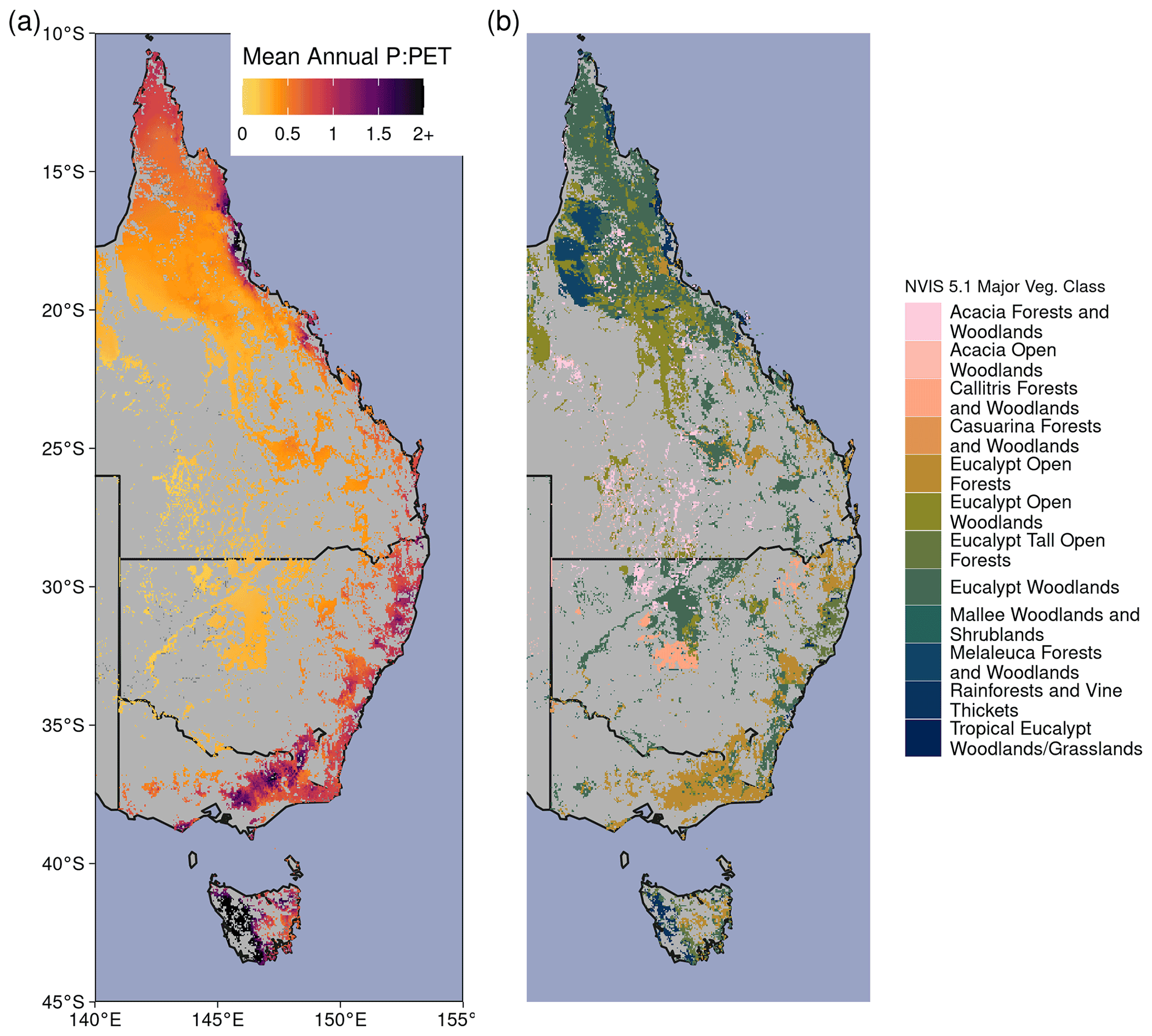
Figure A1(a) Mean Annual P : PET between 1982–2019. (b) Forest and woodland vegetation classes from version 5.1 of the National Vegetation Information System (https://www.environment.gov.au/land/native-vegetation/national-vegetation-information-system, last access: 31 March 2021).
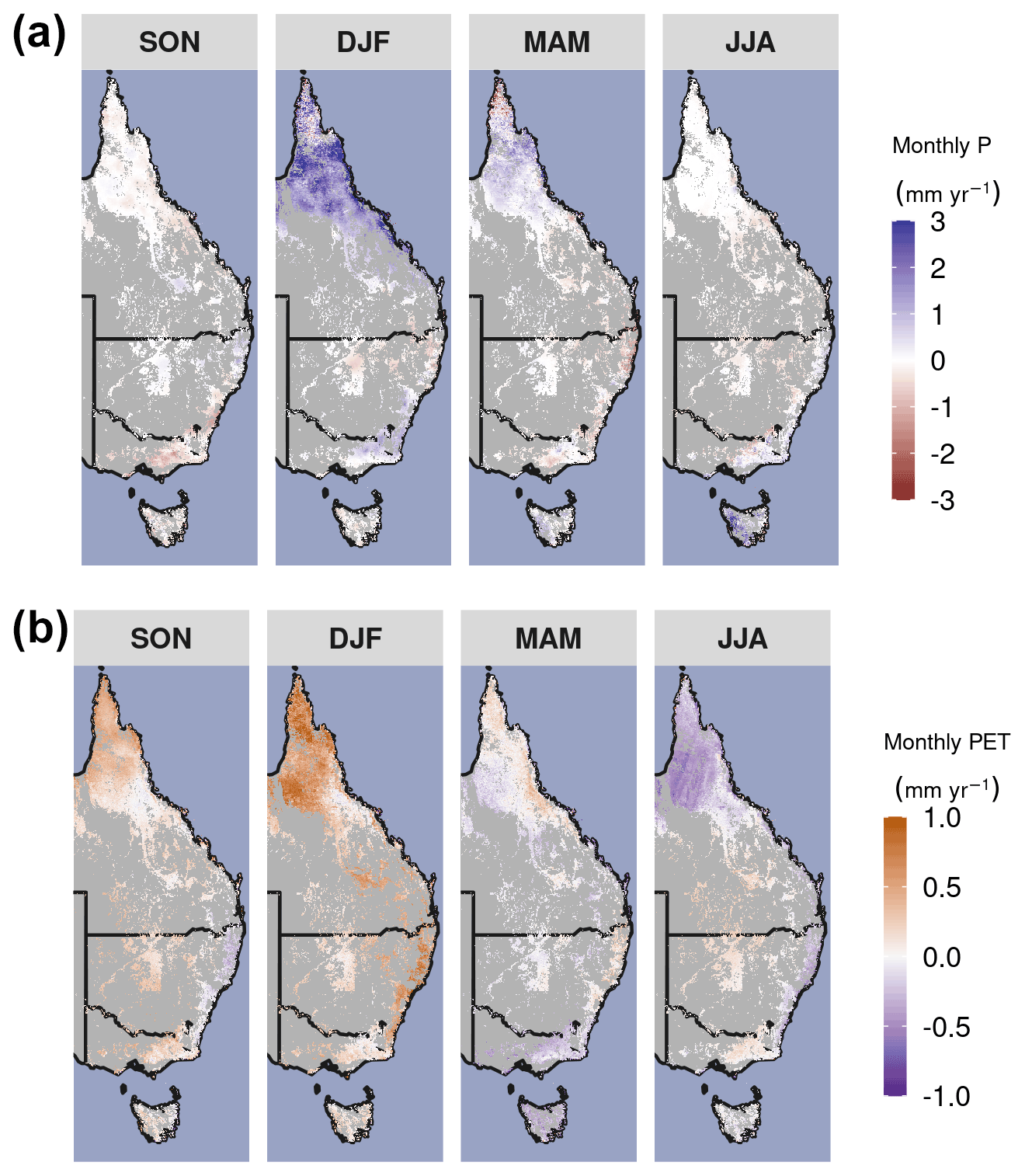
Figure A2Long-term seasonal changes in precipitation (P) and potential evapotranspiration (PET). Linear trend in (a) monthly precipitation and (b) PET by season over the period 1982–2019. Non-forest and woodland regions are masked in gray.
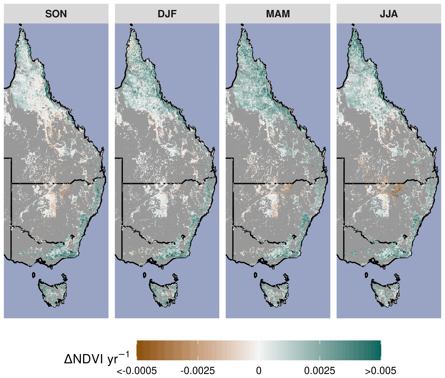
Figure A3The long-term seasonal NDVI linear trend between 1982–2019. The Theil–Sen robust linear trend estimator is used with the calibrated merger of the CDR AVHRR (1982–2000) and MODIS MCD43 (2001–2019) surface reflectance products.
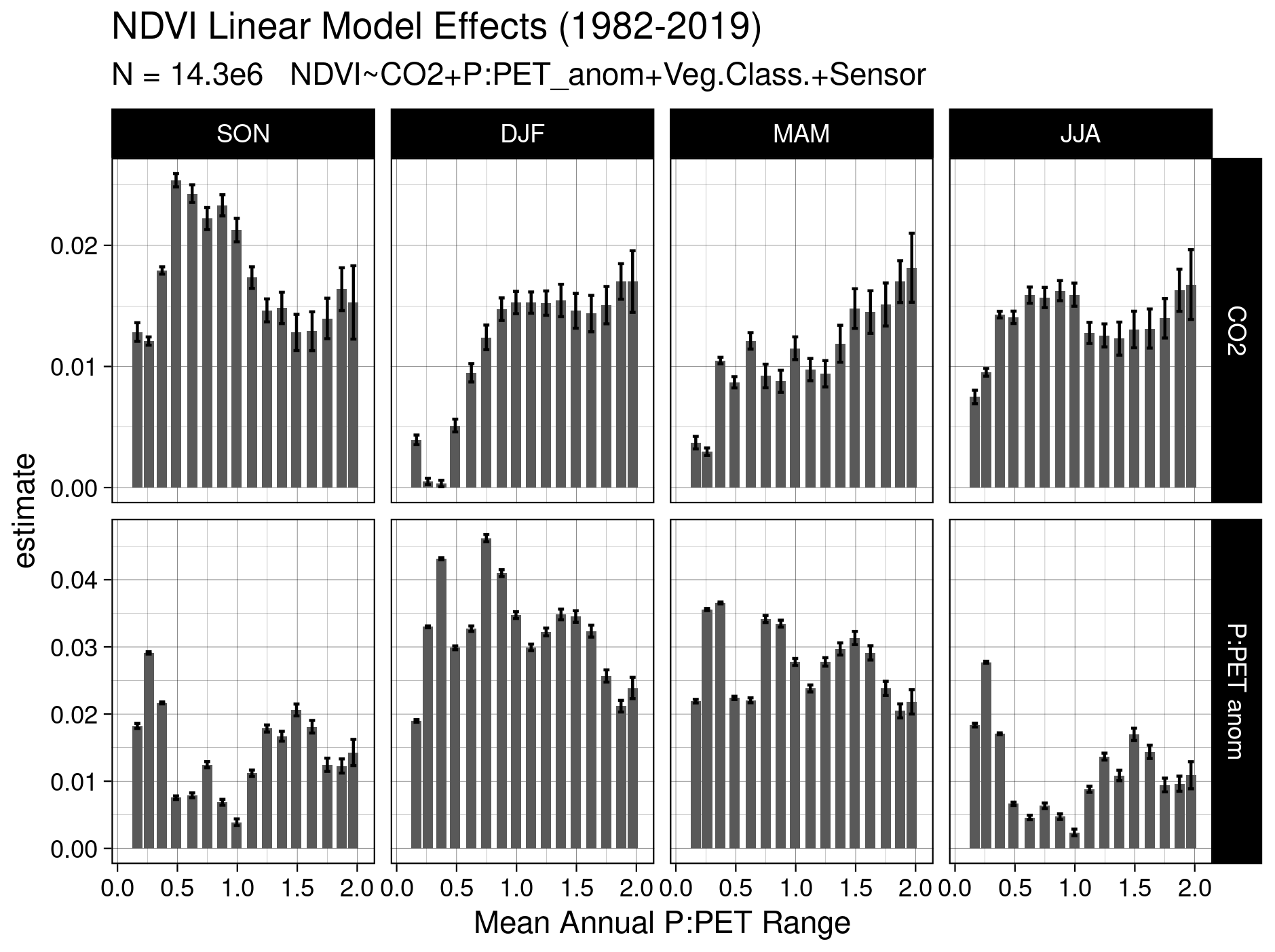
Figure A4Linear model covariate estimates for 128 linear models. The mean annual P : PET range is discretized over 16 increments, where NDVI is modeled as a linear function of CO2, P : PETanom, the NVIS vegetation class, and the sensor. Error bars indicate 2× the standard error in the estimate.
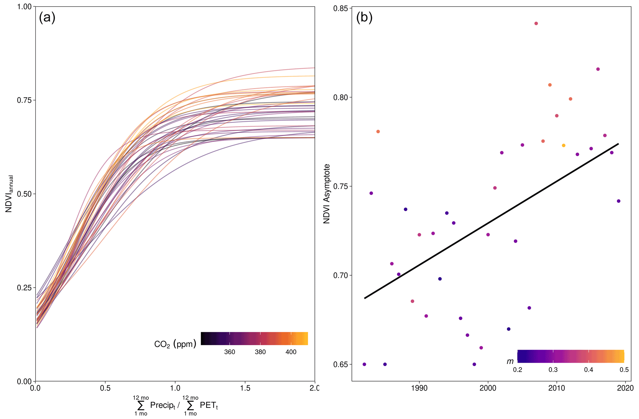
Figure A5NDVI as a logistic function of annual P : PET. (a) Logistic function models, fit per hydrological year. (b) The positive long-term trend in the NDVI asymptote from the logistic model fits; m is the value of P : PET at the inflection point, and “NDVI Asymptote” corresponds to the VA parameter in Eq. (5).
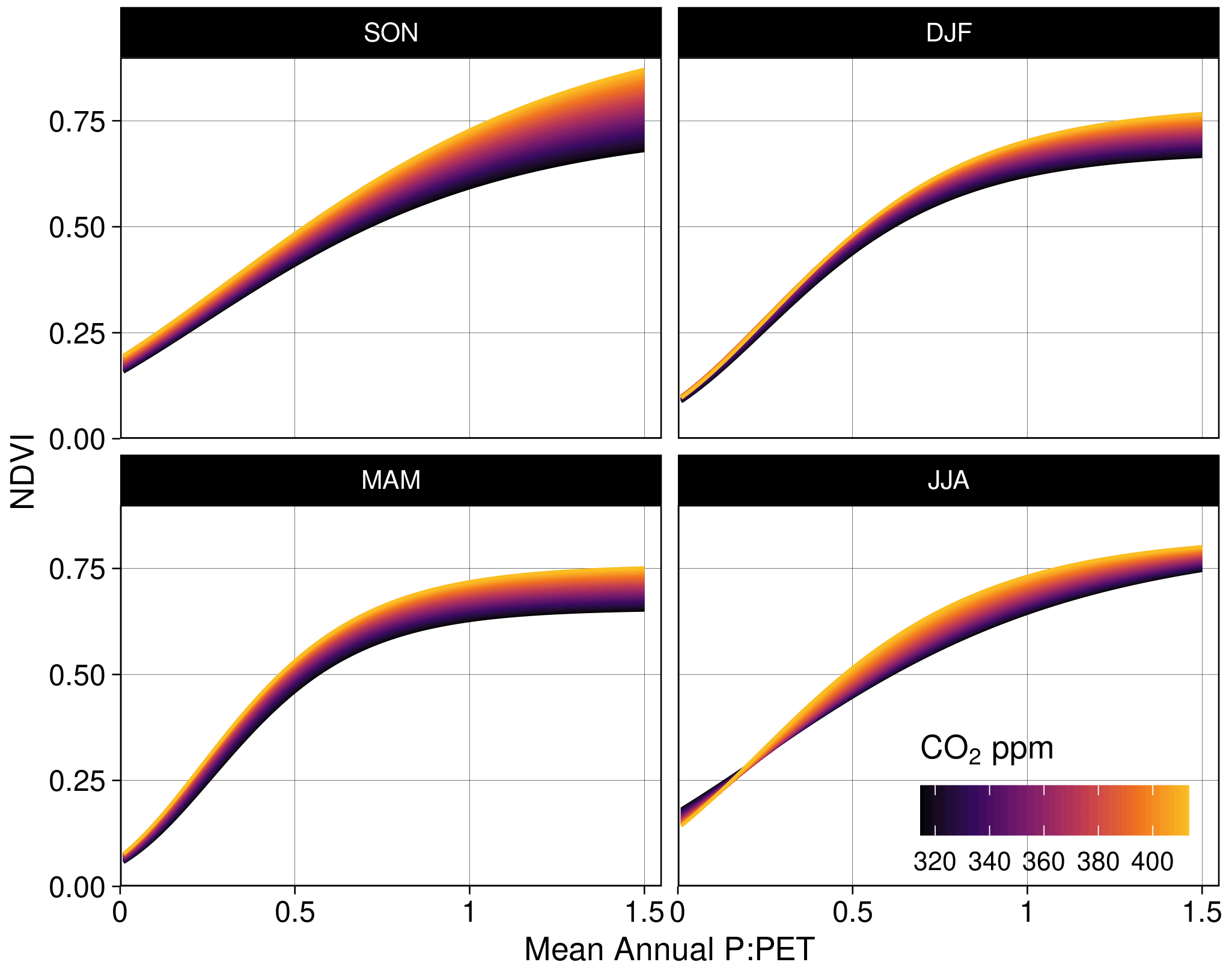
Figure A6Seasonal NDVI as a Richards growth function with linear modifiers of CO2 and the anomaly of P : PET (Eq. 6).
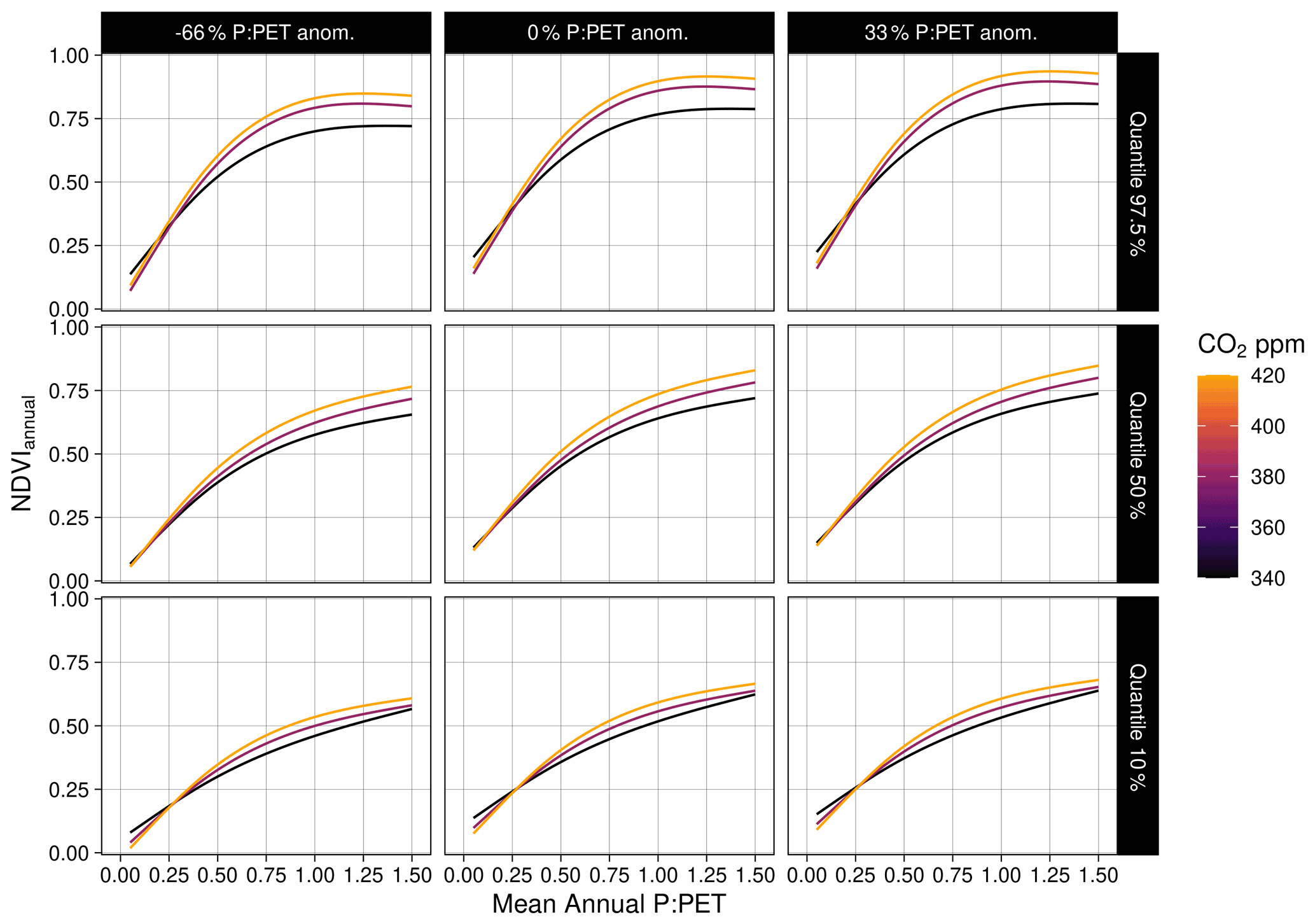
Figure A7Quantile GAM regression predictions across CO2 and anomalies of annual P : PET. NDVI. Here “s” represents a thin plate spline smoothing function, is the 30-year mean annual P : PET, and is the annual anomaly of .
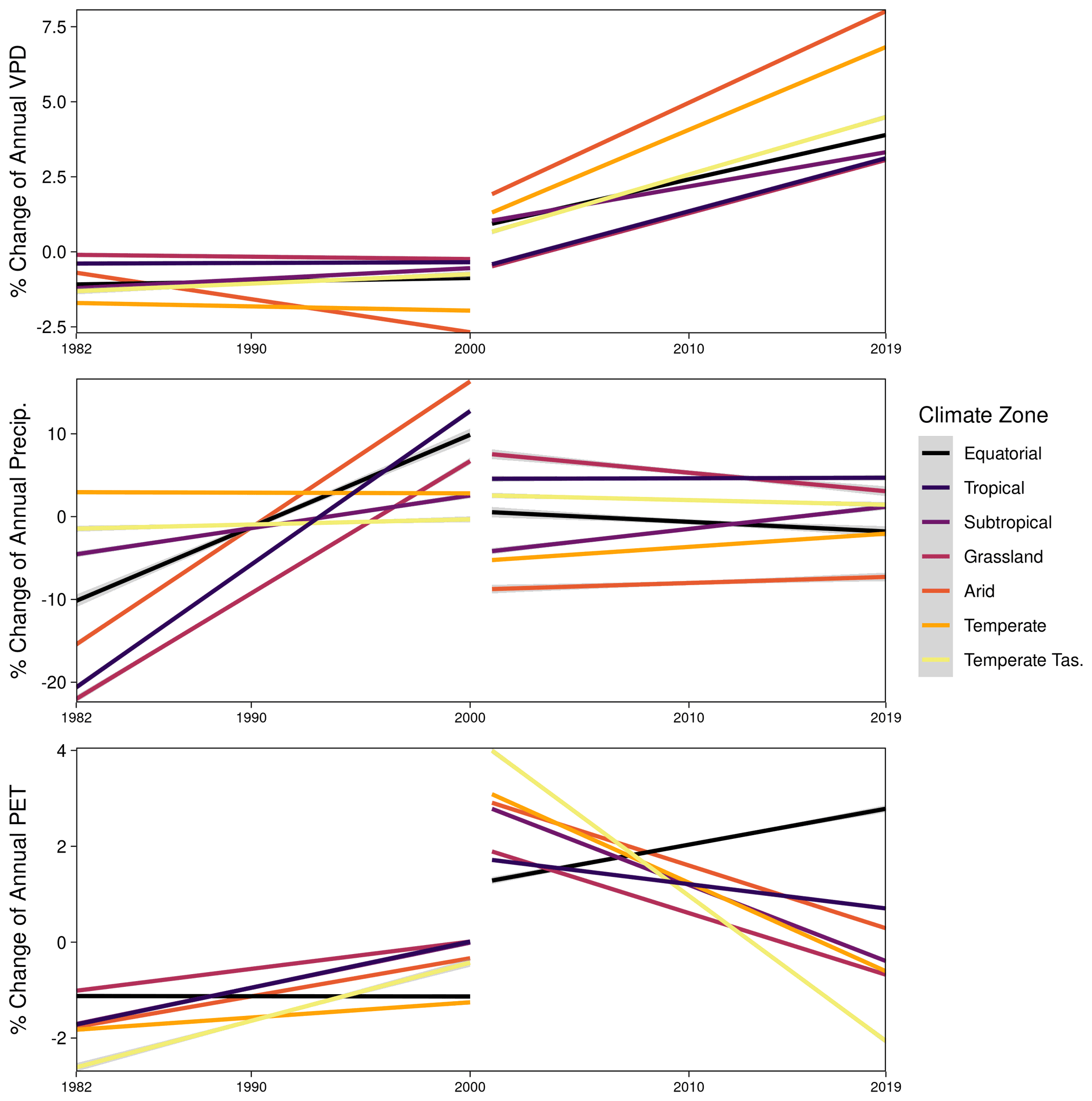
Figure A8The linear relative changes in annual vapor pressure deficit (VPD), precipitation (Precip.), and potential evapotranspiration (PET) by climate zone between satellite epochs AVHRR 1982–2000 and MODIS 2001–2019, as estimated by robust regression. The relative changes are with respect to a climatology period calculated between 1982–2011.
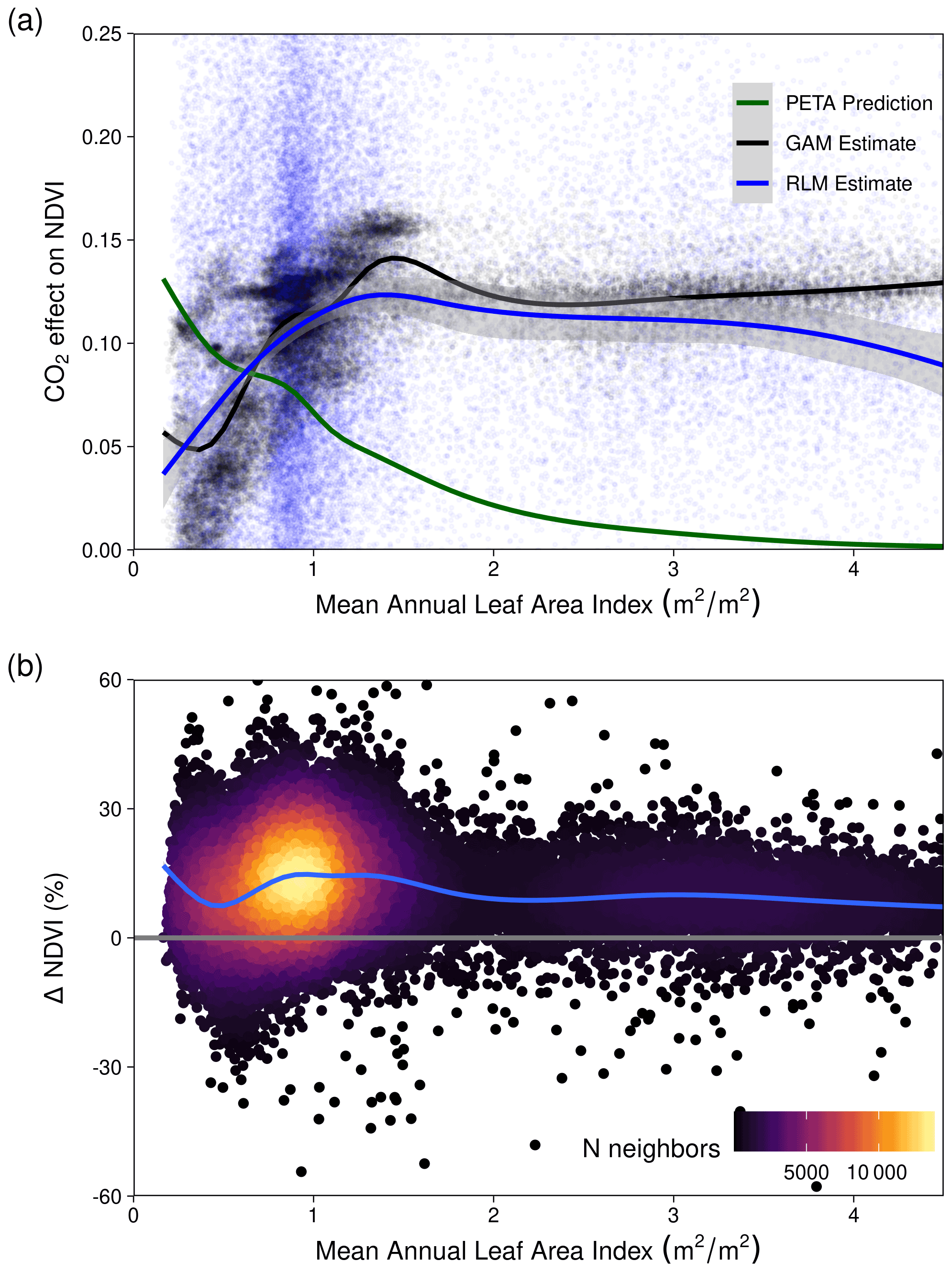
Figure A9(a) The fractional increase in NDVI from CO2 is plotted following predictions from the partitioning of equilibrium transpiration and assimilation (PETA) hypothesis (green), the Generalized Additive Model (GAM; see “Methods”, Eq. 6) estimates, and the pixel-level Robust Linear Model (RLM; see “Methods”, Eq. 5) estimates. Note that we substitute NDVI for the leaf area formulation of the PETA hypothesis (Donohue et al., 2017) because we assume a linear relationship between relative NDVI increase and relative leaf area increase (Donohue et al., 2013; Carlson and Ripley, 1997). (b) The relative change in NDVI between 1982–2019 across the range of mean annual leaf area index calculated with MCD15A3H from 2002–2019.
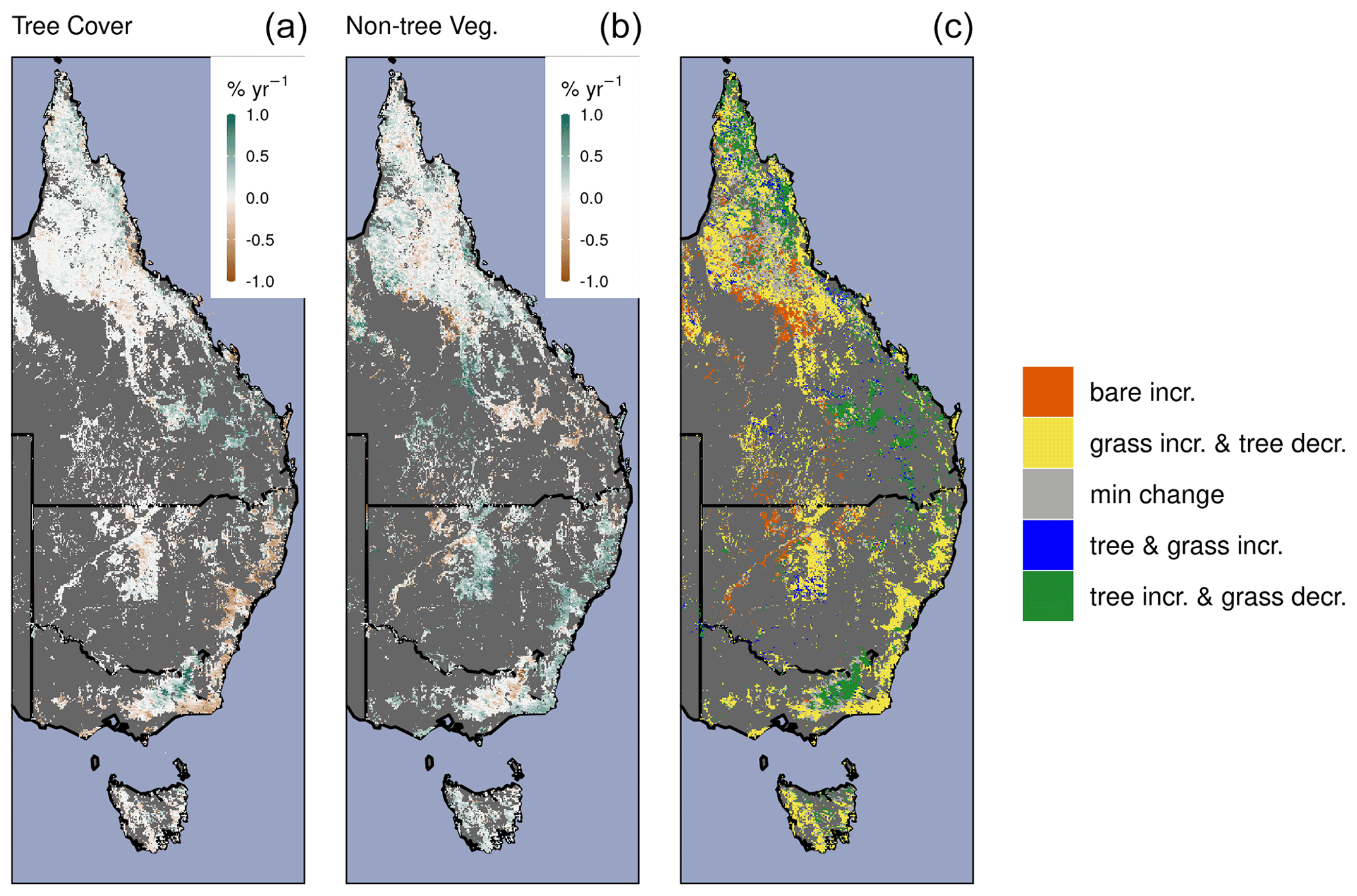
Figure A10The relative shifts in land fraction by tree cover, non-tree vegetation cover (predominantly grasses), and bare ground. Annual rate (2000–2018) of change for tree cover (a), non-tree vegetation (b), and discretized change classes (c). Min change indicates that the annual rate of change in percentage cover was between −0.1 % yr−1 and 0.1 % yr−1.
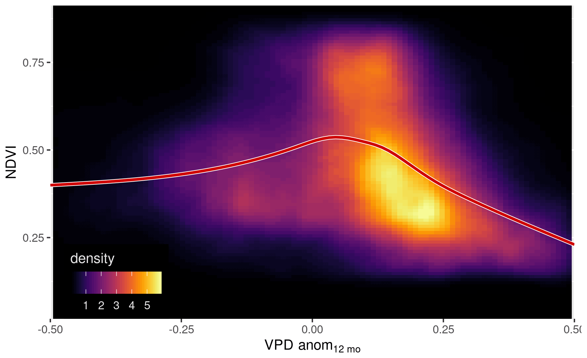
Figure A11The nonlinear dependency of NDVI upon the annual anomaly of vapor pressure deficit. Two-dimensional density plot of NDVI and the running 12-month anomaly of vapor pressure deficit. The red line shows a GAM fit.
All data used are publicly available from sources listed in Table A1. A Git repository with all associated data processing, analysis, and code to reproduce figures is located at https://github.com/sw-rifai/eastern-Australia-CO2-NDVI-change (last access: 18 November 2021) and https://doi.org/10.5281/zenodo.5711964 (Rifai, 2021a). Processed data used in model fitting and figures can be accessed via the Zenodo data repository: https://doi.org/10.5281/zenodo.4340064 (Rifai, 2021b).
SWR, MGDK, PM, LAC, BEM, and AJP designed the study. SWR analyzed the data and produced the figures. SWR and AMU processed climate data. SWR wrote the first draft with MGDK, and all authors have contributed to writing and revising the manuscript.
At least one of the (co-)authors is a member of the editorial board of Biogeosciences. The peer-review process was guided by an independent editor, and the authors also have no other competing interests to declare.
Publisher’s note: Copernicus Publications remains neutral with regard to jurisdictional claims in published maps and institutional affiliations.
We are grateful to Randall J. Donohue (CSIRO Land and Water) for valuable discussion and comments on drafts of this paper.
Sami W. Rifai, Martin G. De Kauwe, Andy J. Pitman, Lucas A. Cernusak, and Patrick Meir received support from the Australian Research Council Discovery Grant (DP190101823). Sami W. Rifai, Martin G. De Kauwe, Anna M. Ukkola, and Andy J. Pitman received support from the ARC Centre of Excellence for Climate Extremes (CE170100023). Martin G. De Kauwe was also supported by the NSW Research Attraction and Acceleration Program and Anna M. Ukkola by an ARC Discovery Early Career Researcher Award (DE200100086). Belinda E. Medlyn received support from the ARC Laureate Fellowship FL190100003.
This paper was edited by Serita Frey and reviewed by two anonymous referees.
Ackerman, D., Millet, D. B., and Chen, X.: Global Estimates of Inorganic Nitrogen Deposition Across Four Decades, Global Biogeochem. Cy., 33, 100–107, https://doi.org/10.1029/2018GB005990, 2019. a
Adzhar, R., Kelley, D. I., Dong, N., Torello Raventos, M., Veenendaal, E., Feldpausch, T. R., Philips, O. L., Lewis, S., Sonké, B., Taedoumg, H., Schwantes Marimon, B., Domingues, T., Arroyo, L., Djagbletey, G., Saiz, G., and Gerard, F.: Assessing MODIS Vegetation Continuous Fields tree cover product (collection 6): performance and applicability in tropical forests and savannas, Biogeosciences Discuss. [preprint], https://doi.org/10.5194/bg-2020-460, in review, 2021. a
Ahlstrom, A., Raupach, M. R., Schurgers, G., Smith, B., Arneth, A., Jung, M., Reichstein, M., Canadell, J. G., Friedlingstein, P., Jain, A. K., Kato, E., Poulter, B., Sitch, S., Stocker, B. D., Viovy, N., Wang, Y. P., Wiltshire, A., Zaehle, S., and Zeng, N.: The Dominant Role of Semi-Arid Ecosystems in the Trend and Variability of the Land CO2 Sink, Science, 348, 895–899, https://doi.org/10.1126/science.aaa1668, 2015. a
Ainsworth, E. A. and Rogers, A.: The Response of Photosynthesis and Stomatal Conductance to Rising [CO2]: Mechanisms and Environmental Interactions: Photosynthesis and Stomatal Conductance Responses to Rising [CO2], Plant Cell. Environ., 30, 258–270, https://doi.org/10.1111/j.1365-3040.2007.01641.x, 2007. a
Atlas of Living Australia: The Dead Tree Detective| Project|BioCollect, available at: https://biocollect.ala.org.au/acsa/project/index/77285a13-e231-49e8-b212-660c66c74bac (last access: 28 November 2020), 2020. a
Australian Department of Agriculture, Water and the Environment: Australian Department of Agriculture, Water and the Environment, available at: http://www.environment.gov.au/ (last access: 31 March 2021), 2020. a
Bastos, A., Running, S. W., Gouveia, C., and Trigo, R. M.: The global NPP dependence on ENSO: La Niña and the extraordinary year of 2011, J. Geophys. Res.-Biogeo., 118, 1247–1255, https://doi.org/10.1002/jgrg.20100, 2013. a
Bronaugh, D. and Werner, A. (for the Pacific Climate Impacts Consortium): Zyp: Zhang + Yue-Pilon Trends Package, available at: https://CRAN.R-project.org/package=zyp (last access: 24 January 2022), 2019. a
Bureau of Meteorology: Annual Australian Climate Statement 2019, available at: http://www.bom.gov.au/climate/current/annual/aus/2019/ (last access: 24 October 2020), 2019. a
Carlson, T. N. and Ripley, D. A.: On the Relation between NDVI, Fractional Vegetation Cover, and Leaf Area Index, Remote Sens. Environ., 62, 241–252, https://doi.org/10.1016/S0034-4257(97)00104-1, 1997. a, b
Cortés, J., Mahecha, M. D., Reichstein, M., Myneni, R. B., Chen, C., and Brenning, A.: Where Are Global Vegetation Greening and Browning Trends Significant?, Geophys. Res. Lett., 48, e2020GL091496, https://doi.org/10.1029/2020GL091496, 2021. a
CSIRO and Bureau of Meteorology: State of the Climate 2020, available at: https://www.csiro.au/-/media/OnA/Files/State-of-the-Climate-2020.pdf (last access: 12 November 2020), 2020. a
Davis, T. W., Prentice, I. C., Stocker, B. D., Thomas, R. T., Whitley, R. J., Wang, H., Evans, B. J., Gallego-Sala, A. V., Sykes, M. T., and Cramer, W.: Simple process-led algorithms for simulating habitats (SPLASH v.1.0): robust indices of radiation, evapotranspiration and plant-available moisture, Geosci. Model Dev., 10, 689–708, https://doi.org/10.5194/gmd-10-689-2017, 2017. a
De Kauwe, M. G., Medlyn, B. E., Zaehle, S., Walker, A. P., Dietze, M. C., Wang, Y.-P., Luo, Y., Jain, A. K., El-Masri, B., Hickler, T., Wå rlind, D., Weng, E., Parton, W. J., Thornton, P. E., Wang, S., Prentice, I. C., Asao, S., Smith, B., McCarthy, H. R., Iversen, C. M., Hanson, P. J., Warren, J. M., Oren, R., and Norby, R. J.: Where Does the Carbon Go? A Model-Data Intercomparison of Vegetation Carbon Allocation and Turnover Processes at Two Temperate Forest Free-Air CO2 Enrichment Sites, New Phytol., 203, 883–899, https://doi.org/10.1111/nph.12847, 2014. a
De Kauwe, M. G., Medlyn, B. E., Ukkola, A. M., Mu, M., Sabot, M. E. B., Pitman, A. J., Meir, P., Cernusak, L. A., Rifai, S. W., Choat, B., Tissue, D. T., Blackman, C. J., Li, X., Roderick, M., and Briggs, P. R.: Identifying Areas at Risk of Drought-induced Tree Mortality across South-Eastern Australia, Glob. Change Biol., 26, 5716–5733, https://doi.org/10.1111/gcb.15215, 2020. a
DiMiceli, C., Carroll, R., Sohlberg, D., Kim, M., and Townshend, J.: MOD44B MODIS/Terra Vegetation Continuous Fields Yearly L3 Global 250 m SIN Grid V006, NASA EOSDIS Land Processes DAAC [data set], https://doi.org/10.5067/MODIS/MOD44B.006, 2017. a, b
Donohue, R. J., McVICAR, T. R., and Roderick, M. L.: Climate-Related Trends in Australian Vegetation Cover as Inferred from Satellite Observations, 1981–2006, Glob. Change Biol., 15, 1025–1039, https://doi.org/10.1111/j.1365-2486.2008.01746.x, 2009. a, b, c
Donohue, R. J., Roderick, M. L., McVicar, T. R., and Farquhar, G. D.: Impact of CO2 fertilization on maximum foliage cover across the globe's warm, arid environments, Geophys. Res. Lett., 40, 3031–3035, https://doi.org/10.1002/grl.50563, 2013. a, b, c, d
Donohue, R. J., Roderick, M. L., McVicar, T. R., and Yang, Y.: A simple hypothesis of how leaf and canopy-level transpiration and assimilation respond to elevated CO2 reveals distinct response patterns between disturbed and undisturbed vegetation, J. Geophys. Res.-Biogeo., 122, 168–184, https://doi.org/10.1002/2016JG003505, 2017. a, b, c
Dowle, M. and Srinivasan, A.: Data.Table: Extension of “data.Frame”, R package version 1.14.0, available at: https://CRAN.R-project.org/package=data.table (last access: 24 January 2022), 2019. a
Drake, B. G., Gonzàlez-Meler, M. A., and Long, S. P.: MORE EFFICIENT PLANTS: A Consequence of Rising Atmospheric CO2?, Annu. Rev. Plant Phys., 48, 609–639, https://doi.org/10.1146/annurev.arplant.48.1.609, 1997. a
Drake, J. E., Macdonald, C. A., Tjoelker, M. G., Crous, K. Y., Gimeno, T. E., Singh, B. K., Reich, P. B., Anderson, I. C., and Ellsworth, D. S.: Short-term carbon cycling responses of a mature eucalypt woodland to gradual stepwise enrichment of atmospheric CO2 concentration, Glob. Change Biol., 22, 380–390, https://doi.org/10.1111/gcb.13109, 2016. a
Evans, M. C.: Deforestation in Australia: drivers, trends and policy responses, Pacific Conservation Biology, 22, 130–150, https://doi.org/10.1071/PC15052, 2016. a
Frankenberg, C., Yin, Y., Byrne, B., He, L., and Gentine, P.: Comment on “Recent Global Decline of CO2 Fertilization Effects on Vegetation Photosynthesis”, Science, 373, eabg2947, https://doi.org/10.1126/science.abg2947, 2021. a, b
Giglio, L., Boschetti, L., Roy, D. P., Humber, M. L., and Justice, C. O.: The Collection 6 MODIS Burned Area Mapping Algorithm and Product, Remote Sens. Environ., 217, 72–85, https://doi.org/10.1016/j.rse.2018.08.005, 2018. a, b
Gill, T., Johansen, K., Phinn, S., Trevithick, R., Scarth, P., and Armston, J.: A Method for Mapping Australian Woody Vegetation Cover by Linking Continental-Scale Field Data and Long-Term Landsat Time Series, Int. J. Remote Sens., 38, 679–705, https://doi.org/10.1080/01431161.2016.1266112, 2017. a
Gorelick, N., Hancher, M., Dixon, M., Ilyushchenko, S., Thau, D., and Moore, R.: Google Earth Engine: Planetary-Scale Geospatial Analysis for Everyone, Remote Sens. Environ., 202, 18–27, https://doi.org/10.1016/j.rse.2017.06.031, 2017. a
Greve, P., Roderick, M. L., Ukkola, A. M., and Wada, Y.: The Aridity Index under Global Warming, Environ. Res. Lett., 14, 124006, https://doi.org/10.1088/1748-9326/ab5046, 2019. a
Hansen, M. C., Potapov, P. V., Moore, R., Hancher, M., Turubanova, S. A., Tyukavina, A., Thau, D., Stehman, S. V., Goetz, S. J., Loveland, T. R., Kommareddy, A., Egorov, A., Chini, L., Justice, C. O., and Townshend, J. R. G.: High-Resolution Global Maps of 21st-Century Forest Cover Change, Science, 342, 850–853, https://doi.org/10.1126/science.1244693, 2013. a
Harris, I., Jones, P., Osborn, T., and Lister, D.: Updated High-Resolution Grids of Monthly Climatic Observations – the CRU TS3.10 Dataset: UPDATED HIGH-RESOLUTION GRIDS OF MONTHLY CLIMATIC OBSERVATIONS, Int. J. Climatol., 34, 623–642, https://doi.org/10.1002/joc.3711, 2014. a
Harris, R. M. B., Beaumont, L. J., Vance, T. R., Tozer, C. R., Remenyi, T. A., Perkins-Kirkpatrick, S. E., Mitchell, P. J., Nicotra, A. B., McGregor, S., Andrew, N. R., Letnic, M., Kearney, M. R., Wernberg, T., Hutley, L. B., Chambers, L. E., Fletcher, M.-S., Keatley, M. R., Woodward, C. A., Williamson, G., Duke, N. C., and Bowman, D. M. J. S.: Biological Responses to the Press and Pulse of Climate Trends and Extreme Events, Nat. Clim. Change, 8, 579–587, https://doi.org/10.1038/s41558-018-0187-9, 2018. a
Hasegawa, S., Macdonald, C. A., and Power, S. A.: Elevated Carbon Dioxide Increases Soil Nitrogen and Phosphorus Availability in a Phosphorus-Limited Eucalyptus Woodland, Glob. Change Biol., 22, 1628–1643, https://doi.org/10.1111/gcb.13147, 2016. a
Hattersley, P. W.: The Distribution of C3 and C4 Grasses in Australia in Relation to Climate, Oecologia, 57, 113–128, https://doi.org/10.1007/BF00379569, 1983. a
Ji, L. and Brown, J. F.: Effect of NOAA Satellite Orbital Drift on AVHRR-Derived Phenological Metrics, Int. J. Appl. Earth Obs., 62, 215–223, https://doi.org/10.1016/j.jag.2017.06.013, 2017. a, b
Jiang, M., Caldararu, S., Zhang, H., Fleischer, K., Crous, K. Y., Yang, J., De Kauwe, M. G., Ellsworth, D. S., Reich, P. B., Tissue, D. T., Zaehle, S., and Medlyn, B. E.: Low Phosphorus Supply Constrains Plant Responses to Elevated CO2: A Meta-analysis, Glob. Change Biol., 26, 5856–5873, https://doi.org/10.1111/gcb.15277, 2020a. a
Jiang, M., Medlyn, B. E., Drake, J. E., Duursma, R. A., Anderson, I. C., Barton, C. V. M., Boer, M. M., Carrillo, Y., Castañeda Gómez, L., Collins, L., Crous, K. Y., De Kauwe, M. G., dos Santos, B. M., Emmerson, K. M., Facey, S. L., Gherlenda, A. N., Gimeno, T. E., Hasegawa, S., Johnson, S. N., Kännaste, A., Macdonald, C. A., Mahmud, K., Moore, B. D., Nazaries, L., Neilson, E. H. J., Nielsen, U. N., Niinemets, U., Noh, N. J., Ochoa-Hueso, R., Pathare, V. S., Pendall, E., Pihlblad, J., Piñeiro, J., Powell, J. R., Power, S. A., Reich, P. B., Renchon, A. A., Riegler, M., Rinnan, R., Rymer, P. D., Salomón, R. L., Singh, B. K., Smith, B., Tjoelker, M. G., Walker, J. K. M., Wujeska-Klause, A., Yang, J., Zaehle, S., and Ellsworth, D. S.: The Fate of Carbon in a Mature Forest under Carbon Dioxide Enrichment, Nature, 580, 227–231, https://doi.org/10.1038/s41586-020-2128-9, 2020b. a, b, c, d
Jones, D., Wang, W., and Fawcett, R.: High-Quality Spatial Climate Data-Sets for Australia, Aust. Meteorol. Ocean., 58, 233–248, 2009. a, b
King, A. D., Pitman, A. J., Henley, B. J., Ukkola, A. M., and Brown, J. R.: The Role of Climate Variability in Australian Drought, Nat. Clim. Change, 10, 177–179, https://doi.org/10.1038/s41558-020-0718-z, 2020. a
Knapp, A. K., Chen, A., Griffin-Nolan, R. J., Baur, L. E., Carroll, C. J., Gray, J. E., Hoffman, A. M., Li, X., Post, A. K., Slette, I. J., Collins, S. L., Luo, Y., and Smith, M. D.: Resolving the Dust Bowl Paradox of Grassland Responses to Extreme Drought, P. Natl. Acad. Sci. USA, 117, 22249–22255, https://doi.org/10.1073/pnas.1922030117, 2020. a
Liao, Z., Van Dijk, A. I. J. M., He, B., Larraondo, P. R., and Scarth, P. F.: Woody Vegetation Cover, Height and Biomass at 25-m Resolution across Australia Derived from Multiple Site, Airborne and Satellite Observations, Int. J. Appl. Earth Obs., 93, 102209, https://doi.org/10.1016/j.jag.2020.102209, 2020. a
McAlpine, C. A., Etter, A., Fearnside, P. M., Seabrook, L., and Laurance, W. F.: Increasing World Consumption of Beef as a Driver of Regional and Global Change: A Call for Policy Action Based on Evidence from Queensland (Australia), Colombia and Brazil, Global Environ. Chang., 19, 21–33, https://doi.org/10.1016/j.gloenvcha.2008.10.008, 2009. a
McMurtrie, R. E., Norby, R. J., Medlyn, B. E., Dewar, R. C., Pepper, D. A., Reich, P. B., Barton, C. V. M., McMurtrie, R. E., Norby, R. J., Medlyn, B. E., Dewar, R. C., Pepper, D. A., Reich, P. B., and Barton, C. V. M.: Why Is Plant-Growth Response to Elevated CO2 Amplified When Water Is Limiting, but Reduced When Nitrogen Is Limiting? A Growth-Optimisation Hypothesis, Funct. Plant Biol., 35, 521–534, https://doi.org/10.1071/FP08128, 2008. a
Medlyn, B. E., Barton, C. V. M., Broadmeadow, M. S. J., Ceulemans, R., Angelis, P. D., Forstreuter, M., Freeman, M., Jackson, S. B., Kellomäki, S., Laitat, E., Rey, A., Roberntz, P., Sigurdsson, B. D., Strassemeyer, J., Wang, K., Curtis, P. S., and Jarvis, P. G.: Stomatal Conductance of Forest Species after Long-Term Exposure to Elevated CO2 Concentration: A Synthesis, New Phytol., 149, 247–264, https://doi.org/10.1046/j.1469-8137.2001.00028.x, 2001. a
Medlyn, B. E., Duursma, R. A., Eamus, D., Ellsworth, D. S., Prentice, I. C., Barton, C. V. M., Crous, K. Y., De Angelis, P., Freeman, M., and Wingate, L.: Reconciling the optimal and empirical approaches to modelling stomatal conductance, Glob. Change Biol., 17, 2134–2144, https://doi.org/10.1111/j.1365-2486.2010.02375.x, 2011. a
Medlyn, B. E., Kauwe, M. G. D., Zaehle, S., Walker, A. P., Duursma, R. A., Luus, K., Mishurov, M., Pak, B., Smith, B., Wang, Y.-P., Yang, X., Crous, K. Y., Drake, J. E., Gimeno, T. E., Macdonald, C. A., Norby, R. J., Power, S. A., Tjoelker, M. G., and Ellsworth, D. S.: Using Models to Guide Field Experiments: A Priori Predictions for the CO2 Response of a Nutrient- and Water-Limited Native Eucalypt Woodland, Glob. Change Biol., 22, 2834–2851, https://doi.org/10.1111/gcb.13268, 2016. a, b
Milly, P. C. D. and Dunne, K. A.: Potential Evapotranspiration and Continental Drying, Nat. Clim. Change, 6, 946–949, https://doi.org/10.1038/nclimate3046, 2016. a
Moore, C. E., Brown, T., Keenan, T. F., Duursma, R. A., van Dijk, A. I. J. M., Beringer, J., Culvenor, D., Evans, B., Huete, A., Hutley, L. B., Maier, S., Restrepo-Coupe, N., Sonnentag, O., Specht, A., Taylor, J. R., van Gorsel, E., and Liddell, M. J.: Reviews and syntheses: Australian vegetation phenology: new insights from satellite remote sensing and digital repeat photography, Biogeosciences, 13, 5085–5102, https://doi.org/10.5194/bg-13-5085-2016, 2016. a
Morison, J. I. L.: Sensitivity of Stomata and Water Use Efficiency to High CO2, Plant Cell Environ., 8, 467–474, https://doi.org/10.1111/j.1365-3040.1985.tb01682.x, 1985. a
Muñoz Sabater, J.: ERA5-Land hourly data from 1981 to present, Copernicus Climate Change Service (C3S) Climate Data Store (CDS) [data set], https://doi.org/10.24381/cds.e2161bac, 2019. a
Murphy, B. P. and Bowman, D. M. J. S.: Seasonal Water Availability Predicts the Relative Abundance of C3 and C4 Grasses in Australia, Global Ecol. Biogeogr., 16, 160–169, https://doi.org/10.1111/j.1466-8238.2006.00285.x, 2007. a, b
Myneni, R., Knyazikhin, Y., and Park, T.: MCD15A3H MODIS/Terra+Aqua Leaf Area Index/FPAR 4-day L4 Global 500 m SIN Grid V006, NASA EOSDIS Land Processes DAAC [data set], https://doi.org/10.5067/MODIS/MCD15A3H.006, 2015. a
Nolan, R. H., Boer, M. M., Collins, L., de Dios, V. R., Clarke, H., Jenkins, M., Kenny, B., and Bradstock, R. A.: Causes and Consequences of Eastern Australia's 2019–20 Season of Mega-Fires, Glob. Change Biol., 26, 1039–1041, https://doi.org/10.1111/gcb.14987, 2020. a
Padfield, D. and Matheson, G.: Nls.Multstart: Robust Non-Linear Regression Using AIC Scores, R package version 1.2.0, available at: https://CRAN.R-project.org/package=nls.multstart (last access: 24 January 2022), 2020. a
Pebesma, E.: Stars: Spatiotemporal Arrays, Raster and Vector Data Cubes, GitHub [software], available at: https://r-spatial.github.io/stars/ https://github.com/r-spatial/stars/ (last access: 24 January 2022), 2020. a
Perkins, S. E., Alexander, L. V., and Nairn, J. R.: Increasing Frequency, Intensity and Duration of Observed Global Heatwaves and Warm Spells, Geophys. Res. Lett., 39, L20714, https://doi.org/10.1029/2012GL053361, 2012. a
Peters, J. M. R., López, R., Nolf, M., Hutley, L. B., Wardlaw, T., Cernusak, L. A., and Choat, B.: Living on the Edge: A Continental-Scale Assessment of Forest Vulnerability to Drought, Glob. Change Biol., 27, 3620–3641, https://doi.org/10.1111/gcb.15641, 2021. a
Poulter, B., Frank, D., Ciais, P., Myneni, R. B., Andela, N., Bi, J., Broquet, G., Canadell, J. G., Chevallier, F., Liu, Y. Y., Running, S. W., Sitch, S., and van der Werf, G. R.: Contribution of Semi-Arid Ecosystems to Interannual Variability of the Global Carbon Cycle, Nature, 509, 600–603, https://doi.org/10.1038/nature13376, 2014. a
Raupach, M.: Equilibrium Evaporation and the Convective Boundary Layer, Bound.-Lay. Meteorol., 96, 107–142, 2000. a
Rifai, S. W.: sw-rifai/eastern-Australia-CO2-NDVI-change: revision_1 (revision_1), Zenodo [code, data set], https://doi.org/10.5281/zenodo.5711964, 2021a. a
Rifai, S. W.: Thirty-eight years of CO2 fertilization have outpaced growing aridity to drive greening of Australian woody ecosystems, version 0.1, Zenodo [data set], https://doi.org/10.5281/zenodo.4340064, 2021b. a
Schaaf, C. and Wang, Z.: MCD43A4 MODIS/Terra+Aqua BRDF/Albedo Nadir BRDF Adjusted RefDaily L3 Global – 500 m V006, NASA EOSDIS Land Processes DAAC [data set], https://doi.org/10.5067/MODIS/MCD43A4.006, 2015. a, b
Seabrook, L., McAlpine, C., and Fensham, R.: Cattle, Crops and Clearing: Regional Drivers of Landscape Change in the Brigalow Belt, Queensland, Australia, 1840–2004, Landscape Urban Plan., 78, 373–385, https://doi.org/10.1016/j.landurbplan.2005.11.007, 2006. a
Sexton, J. O., Song, X.-P., Feng, M., Noojipady, P., Anand, A., Huang, C., Kim, D.-H., Collins, K. M., Channan, S., DiMiceli, C., and Townshend, J. R.: Global, 30-m Resolution Continuous Fields of Tree Cover: Landsat-Based Rescaling of MODIS Vegetation Continuous Fields with Lidar-Based Estimates of Error, Int. J. Digit. Earth, 6, 427–448, https://doi.org/10.1080/17538947.2013.786146, 2013. a
Smith, S. D., Charlet, T. N., Zitzer, S. F., Abella, S. R., Vanier, C. H., and Huxman, T. E.: Long-Term Response of a Mojave Desert Winter Annual Plant Community to a Whole-Ecosystem Atmospheric CO2 Manipulation (FACE), Glob. Change Biol., 20, 879–892, https://doi.org/10.1111/gcb.12411, 2014. a
Specht, R.: Water Use by Perennial Evergreen Plant Communities in Australia and Papua New Guinea, Aust. J. Bot., 20, 273–299, https://doi.org/10.1071/BT9720273, 1972. a, b
Teckentrup, L., De Kauwe, M. G., Pitman, A. J., Goll, D. S., Haverd, V., Jain, A. K., Joetzjer, E., Kato, E., Lienert, S., Lombardozzi, D., McGuire, P. C., Melton, J. R., Nabel, J. E. M. S., Pongratz, J., Sitch, S., Walker, A. P., and Zaehle, S.: Assessing the representation of the Australian carbon cycle in global vegetation models, Biogeosciences, 18, 5639–5668, https://doi.org/10.5194/bg-18-5639-2021, 2021. a, b
Trancoso, R., Larsen, J. R., McVicar, T. R., Phinn, S. R., and McAlpine, C. A.: CO2-vegetation Feedbacks and Other Climate Changes Implicated in Reducing Base Flow, Geophys. Res. Lett., 44, 2310–2318, https://doi.org/10.1002/2017GL072759, 2017. a
Ukkola, A. M., Prentice, I. C., Keenan, T. F., van Dijk, A. I. J. M., Viney, N. R., Myneni, R. B., and Bi, J.: Reduced Streamflow in Water-Stressed Climates Consistent with CO2 Effects on Vegetation, Nat. Clim. Change, 6, 75–78, https://doi.org/10.1038/nclimate2831, 2016. a, b, c, d, e, f
Ukkola, A. M., Roderick, M. L., Barker, A., and Pitman, A. J.: Exploring the Stationarity of Australian Temperature, Precipitation and Pan Evaporation Records over the Last Century, Environ. Res. Lett., 14, 124035, https://doi.org/10.1088/1748-9326/ab545c, 2019. a, b
van Dijk, A. I. J. M., Beck, H. E., Crosbie, R. S., de Jeu, R. A. M., Liu, Y. Y., Podger, G. M., Timbal, B., and Viney, N. R.: The Millennium Drought in southeast Australia (2001–2009): Natural and human causes and implications for water resources, ecosystems, economy, and society, Water Resour. Res., 49, 1040–1057, https://doi.org/10.1002/wrcr.20123, 2013. a
Venables, W. N. and Ripley, B. D.: Modern Applied Statistics with S, Springer, 4th Edn., available at: http://www.stats.ox.ac.uk/pub/MASS4 (last access: 24 January 2022), 2002. a
Vermote, E. and NOAA CDR Program: NOAA Climate Data Record (CDR) of AVHRR Surface Reflectance, Version 5, NOAA National Centers for Environmental Information [data set], https://doi.org/10.7289/V53776Z4, 2018. a, b
Walker, A. P., De Kauwe, M. G., Bastos, A., Belmecheri, S., Georgiou, K., Keeling, R. F., McMahon, S. M., Medlyn, B. E., Moore, D. J. P., Norby, R. J., Zaehle, S., Anderson-Teixeira, K. J., Battipaglia, G., Brienen, R. J. W., Cabugao, K. G., Cailleret, M., Campbell, E., Canadell, J. G., Ciais, P., Craig, M. E., Ellsworth, D. S., Farquhar, G. D., Fatichi, S., Fisher, J. B., Frank, D. C., Graven, H., Gu, L., Haverd, V., Heilman, K., Heimann, M., Hungate, B. A., Iversen, C. M., Joos, F., Jiang, M., Keenan, T. F., Knauer, J., Körner, C., Leshyk, V. O., Leuzinger, S., Liu, Y., MacBean, N., Malhi, Y., McVicar, T. R., Penuelas, J., Pongratz, J., Powell, A. S., Riutta, T., Sabot, M. E. B., Schleucher, J., Sitch, S., Smith, W. K., Sulman, B., Taylor, B., Terrer, C., Torn, M. S., Treseder, K. K., Trugman, A. T., Trumbore, S. E., Mantgem, P. J., Voelker, S. L., Whelan, M. E., and Zuidema, P. A.: Integrating the Evidence for a Terrestrial Carbon Sink Caused by Increasing Atmospheric CO2, New Phytol., 229, 2413–2445, https://doi.org/10.1111/nph.16866, 2020. a
Wang, S., Zhang, Y., Ju, W., Chen, J. M., Ciais, P., Cescatti, A., Sardans, J., Janssens, I. A., Wu, M., Berry, J. A., Campbell, E., Fernández-Martínez, M., Alkama, R., Sitch, S., Friedlingstein, P., Smith, W. K., Yuan, W., He, W., Lombardozzi, D., Kautz, M., Zhu, D., Lienert, S., Kato, E., Poulter, B., Sanders, T. G. M., Krüger, I., Wang, R., Zeng, N., Tian, H., Vuichard, N., Jain, A. K., Wiltshire, A., Haverd, V., Goll, D. S., and Peñuelas, J.: Recent Global Decline of CO2 Fertilization Effects on Vegetation Photosynthesis, Science, 370, 1295–1300, https://doi.org/10.1126/science.abb7772, 2020. a, b, c, d
Winkler, A. J., Myneni, R. B., Hannart, A., Sitch, S., Haverd, V., Lombardozzi, D., Arora, V. K., Pongratz, J., Nabel, J. E. M. S., Goll, D. S., Kato, E., Tian, H., Arneth, A., Friedlingstein, P., Jain, A. K., Zaehle, S., and Brovkin, V.: Slowdown of the greening trend in natural vegetation with further rise in atmospheric CO2, Biogeosciences, 18, 4985–5010, https://doi.org/10.5194/bg-18-4985-2021, 2021. a
Wong, S.-C., Cowan, I. R., and Farquhar, G. D.: Leaf Conductance in Relation to Rate of CO2 Assimilation: I. Influence of Nitrogen Nutrition, Phosphorus Nutrition, Photon Flux Density, and Ambient Partial Pressure of CO2 during Ontogeny, Plant Physiol., 78, 821–825, https://doi.org/10.1104/pp.78.4.821, 1985. a
Wood, S. N.: Generalized Additive Models: An Introduction with R, Chapman and Hall/CRC, 2nd Edn., ISBN 978-1-49872-834-8, 2017. a
World Meteorological Organization: WMO Guidelines on the Calculation of Climate Normals, available at: https://library.wmo.int/doc_num.php?explnum_id=4166 (last access: 31 March 2020), 2017. a
Yang, J., Medlyn, B. E., De Kauwe, M. G., and Duursma, R. A.: Applying the Concept of Ecohydrological Equilibrium to Predict Steady State Leaf Area Index, J. Adv. Model. Earth Sy., 10, 1740–1758, https://doi.org/10.1029/2017MS001169, 2018. a
Zhu, Z., Piao, S., Myneni, R. B., Huang, M., Zeng, Z., Canadell, J. G., Ciais, P., Sitch, S., Friedlingstein, P., Arneth, A., Cao, C., Cheng, L., Kato, E., Koven, C., Li, Y., Lian, X., Liu, Y., Liu, R., Mao, J., Pan, Y., Peng, S., Peñuelas, J., Poulter, B., Pugh, T. A. M., Stocker, B. D., Viovy, N., Wang, X., Wang, Y., Xiao, Z., Yang, H., Zaehle, S., and Zeng, N.: Greening of the Earth and Its Drivers, Nat. Clim. Change, 6, 791–795, https://doi.org/10.1038/nclimate3004, 2016. a, b, c, d
Zhu, Z., Zeng, H., Myneni, R. B., Chen, C., Zhao, Q., Zha, J., Zhan, S., and MacLachlan, I.: Comment on “Recent Global Decline of CO2 Fertilization Effects on Vegetation Photosynthesis”, Science, 373, eabg5673, https://doi.org/10.1126/science.abg5673, 2021. a