the Creative Commons Attribution 4.0 License.
the Creative Commons Attribution 4.0 License.
 | 09 Feb 2022
Test-size evolution of the planktonic foraminifer Globorotalia menardii in the eastern tropical Atlantic since the Late Miocene
Thore Friesenhagen
The mean test size of planktonic foraminifera (PF) is known to have increased especially during the last 12 Myr, probably in terms of an adaptive response to an intensification of the surface-water stratification. On geologically short timescales, the test size in PF is related to environmental conditions. In an optimal species-specific environment, individuals exhibit a greater maximum and average test size, while the size decreases the more unfavourable the environment becomes.
An interesting case was observed in the late Neogene and Quaternary size evolution of Globorotalia menardii, which seems to be too extreme to be only explained by changes in environmental conditions. In the western tropical Atlantic Ocean (WTAO) and the Caribbean Sea, the test size more than doubles from 2.6 to 1.95 and 1.7 Ma, respectively, following an almost uninterrupted and successive phase of test-size decrease from 4 Ma. Two hypotheses have been suggested to explain the sudden occurrence of a giant G. menardii form: it was triggered by either (1) a punctuated, regional evolutionary event or (2) the immigration of specimens from the Indian Ocean via the Agulhas leakage.
Morphometric measurements of tests from sediment samples of the Ocean Drilling Program (ODP) Leg 108 Hole 667A in the eastern tropical Atlantic Ocean (ETAO) show that the giant type already appears 0.1 Myr earlier at this location than in the WTAO, which indicates that the extreme size increase in the early Pleistocene was a tropical-Atlantic-Ocean-wide event. A coinciding change in the predominant coiling direction likely suggests that a new morphotype occurred. If the giant size and the uniform change in the predominant coiling direction are an indicator for this new type, the form already occurred in the eastern tropical Pacific Ocean at the Pliocene–Pleistocene boundary at 2.58 Ma. This finding supports the Agulhas leakage hypothesis. However, the hypothesis of a regional, punctuated evolutionary event cannot be dismissed due to missing data from the Indian Ocean.
This paper presents the Atlantic Meridional Overturning Circulation (AMOC) and thermocline hypothesis in the ETAO, which possibly can be extrapolated for explaining the test-size evolution of the whole tropical Atlantic Ocean and the Caribbean Sea for the time interval between 2 and 8 Ma. The test-size evolution shows a similar trend with indicators for changes in the AMOC strength. The mechanism behind this might be that changes in the AMOC strength have a major influence on the thermal stratification of the upper water column and hence the thermocline, which is known to be the habitat of G. menardii.
- Article
(12139 KB) - Full-text XML
-
Supplement
(1190 KB) - BibTeX
- EndNote


While short-term changes in the size of planktonic foraminifera (PF) calcareous skeletons, so-called “tests”, are thought to be related to changes in environmental conditions (Hecht, 1976; Ortiz et al., 1995; Schmidt et al., 2006; Woodhouse et al., 2021), macroevolutionary increase in the test size is primarily associated with evolutionary adaptation to new ecological niches, for example surface-water stratification (Schmidt et al., 2004; Wade et al., 2016).
Knappertsbusch (2007a, 2016) observed interesting long-term test-size evolution of PF in studies of the G. menardii–G. limbata–G. multicamerata lineage from the late Miocene until the present. His studies revealed a striking size increase in G. menardii in the tropical Atlantic Ocean and the Caribbean Sea in the early Pleistocene from 2.6 to 1.95 and 1.7 Ma, respectively. The size more than doubled within this time interval.
Although the maximum average test size of a species is reached in regions which provide optimal species-specific temperatures and salinities on geologically short time intervals (Hecht, 1976; Schmidt et al., 2006), this event seemed to be too pronounced and incisive to only be related to even a drastic improvement of environmental conditions. Therefore, Knappertsbusch argued that this relatively sudden and pronounced increase had been caused by the occurrence of a new giant G. menardii form in the Atlantic Ocean that may be passively entrained from the Indian Ocean, possibly via an intensified “palaeo-Agulhas” leakage after the onset of the Northern Hemisphere Glaciation (NHG). The Agulhas leakage is mediated by the transport of ring-shaped water masses from the Indian Ocean into the Atlantic Ocean, which separates from the Agulhas Current at its retroflection point at the southernmost tip of Africa (Biastoch et al., 2009; Beal et al., 2011; Laxenaire et al., 2018). These Agulhas Rings are known to transport tropical Indian Ocean biota into the Atlantic Ocean (Norris, 1999; Caley et al., 2012; Villar et al., 2015). A similar mechanism has been proposed for the dispersal of giant menardiform specimens ca. 2 Myr ago (Knappertsbusch, 2016).
During the NHG, permanent ice sheets were established in the Northern Hemisphere. The NHG started ca. 2.7 Myr ago, intensified until 1.8 Ma, and has had a major influence on the global climate and environmental conditions (Raymo, 1994; Tiedemann et al., 1994). The closure of the Isthmus of Panama probably triggered and/or intensified the NHG (Haug and Tiedemann, 1998; Bartoli et al., 2005; O'Dea et al., 2016).
Punctuated gradualism (Malmgren et al., 1983), i.e. rapid test-size evolution, comes to mind as an alternative mechanism to explain the observed patterns. It proposes a regional in situ size evolution under changed niche, nutritional or growth conditions of G. menardii after the onset of the NHG and a simultaneously rapid spread within the entire tropical to subtropical Atlantic Ocean.
The present study documents the associated morphological changes. Particularly, it investigates if the pronounced test-size increase in G. menardii observed in the Caribbean Sea (Knappertsbusch, 2007a) and the western tropical Atlantic Ocean (WTAO; Knappertsbusch, 2016) in the early Pleistocene occurs also in the eastern tropical Atlantic Ocean (ETAO). It seeks new insight for the underlying evolutionary processes. The new data from the ETAO will be discussed against the background of the Agulhas leakage hypothesis and the punctuated gradualism hypothesis while acknowledging the fact that neither the location nor the sampling resolution can unequivocally prove the mentioned hypotheses. The data rather give evidence for the likelihood of these hypotheses by extending the morphological dataset of menardiform globorotallids.
This study follows the strategy of “evolutionary prospection” (Knappertsbusch, 2011). Here, the concept of evolutionary prospection is to map morphological variations of tests of the G. menardii lineage within its entire biogeographic range at several different localities through geological time. This global approach and increasing datasets of test-size measurements of menardiform globorotallids for the last 8 Myr hopefully allow us to disentangle and understand the evolutionary processes behind the observed pattern and general environmental processes influencing test-size evolution.
In this context, a new Atlantic Meridional Overturning Circulation (AMOC) and thermocline hypothesis is proposed, which may explain the evolutionary pattern of the size evolution in the tropical Atlantic during the time interval lasting from 8 to 2 Ma.
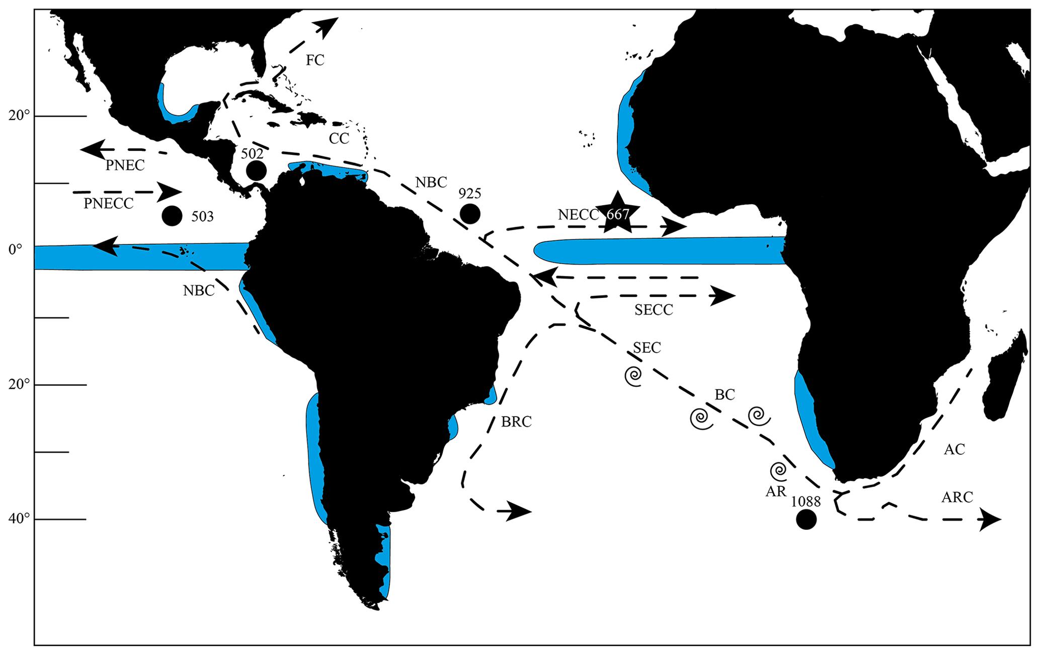
Figure 1Map of the southern and tropical Atlantic Ocean showing the investigated and other important sites, as well as the most important currents. The star marks Site 667 and the black dots Sites 502, 503 and 925, which were investigated by Knappertsbusch (2007a, 2016), as well as ODP Site 1088, which was used by Dausmann et al. (2017) for a reconstruction of the AMOC strength using εNd isotopes. Blue areas show regions of upwelling (Shipboard Scientific Party, 1998, 2003; Merino and Monreal-Gómez, 2009; Clyde-Brockway, 2014; Pelegrí and Benazzouz, 2015; Kämpf and Chapman, 2016). Currents following Shipboard Scientific Party (1998). AC = Agulhas Current, AR = Agulhas Rings, ARC = Agulhas Return Current, BC = Benguela Current, BRC = Brazil Current, CC = Caribbean Current, FC = Florida Current, NBC = North Brazil Current, NECC = North Equatorial Counter Current, PNEC = Pacific North Equatorial Current, PNECC = Pacific North Equatorial Counter Current, SEC = South Equatorial Current, SECC = South Equatorial Counter Current.
2.1 ODP Hole 667A
Ocean Drilling Program (ODP) Hole 667A was visited during Leg 108 and is located at the Sierra Leone Rise in the eastern equatorial Atlantic Ocean (4∘34.15′ N, 21∘54.68′ W; Fig. 1). Several characteristics qualify this site for being investigated in terms of the test-size increase event of G. menardii in the early Pleistocene:
-
This area is located within tropical waters, the known habitat for G. menardii (Caley et al., 2012). Surface sediments show that G. menardii has a high Holocene occurrence at this site. Throughout the studied interval, sediments contain an adequate number of G. menardii and related forms (Manivit, 1989). The core location is outside or within the peripheral northwest African upwelling system (Fig. 1) and therefore only marginally affected by the system for the investigated time interval of the last 8 Myr (Weaver and Raymo, 1989). Thus, there is a relatively long-term water-column stability on the geological timescale at ODP Site 667.
-
This area is within the range of water masses which are affected by the Agulhas leakage (Biastoch et al., 2009; Rühs et al., 2013) so that biota originating in the Indian Ocean are transported by currents up to this location.
-
The preservation of the fossils is good to moderate (Manivit, 1989). It is partly attributed to a sediment deposition depth (present: 3529.3 m water depth below sea level) above the carbonate compensation depth, i.e. the water depth in the ocean, at which the rate of calcium carbonate supply equals the rate of calcium carbonate dissolution and below which no calcite is preserved.
-
For the studied interval from 8 Ma until the present, sedimentation has most likely been continuous. The sediment sequence is only disturbed by a small slump (Shipboard Scientific Party, 1988), which was avoided for sampling.
2.2 Sample selection
The samples were chosen from interglacial periods with a similar age as the investigated samples of the studies of Knappertsbusch (2007a, 2016) (Table 1). The working hypothesis presumes G. menardii to reach its maximum test size during interglacials, inferred from the observation of an overall decrease in population size or even complete absence during glacial intervals in the Atlantic Ocean (Ericson and Wollin, 1956; Sexton and Norris, 2011, and references therein; Portilho-Ramos et al., 2014).
Table 1Studied samples, their depths in metres below seafloor (m b.s.f.) and age (Ma; Neptune model 0667A.loc95 (using magnetostratigraphic, planktonic foraminiferal and calcareous nannofossil data)) of Hole 667A, following the age depth plot of Fig. 2.
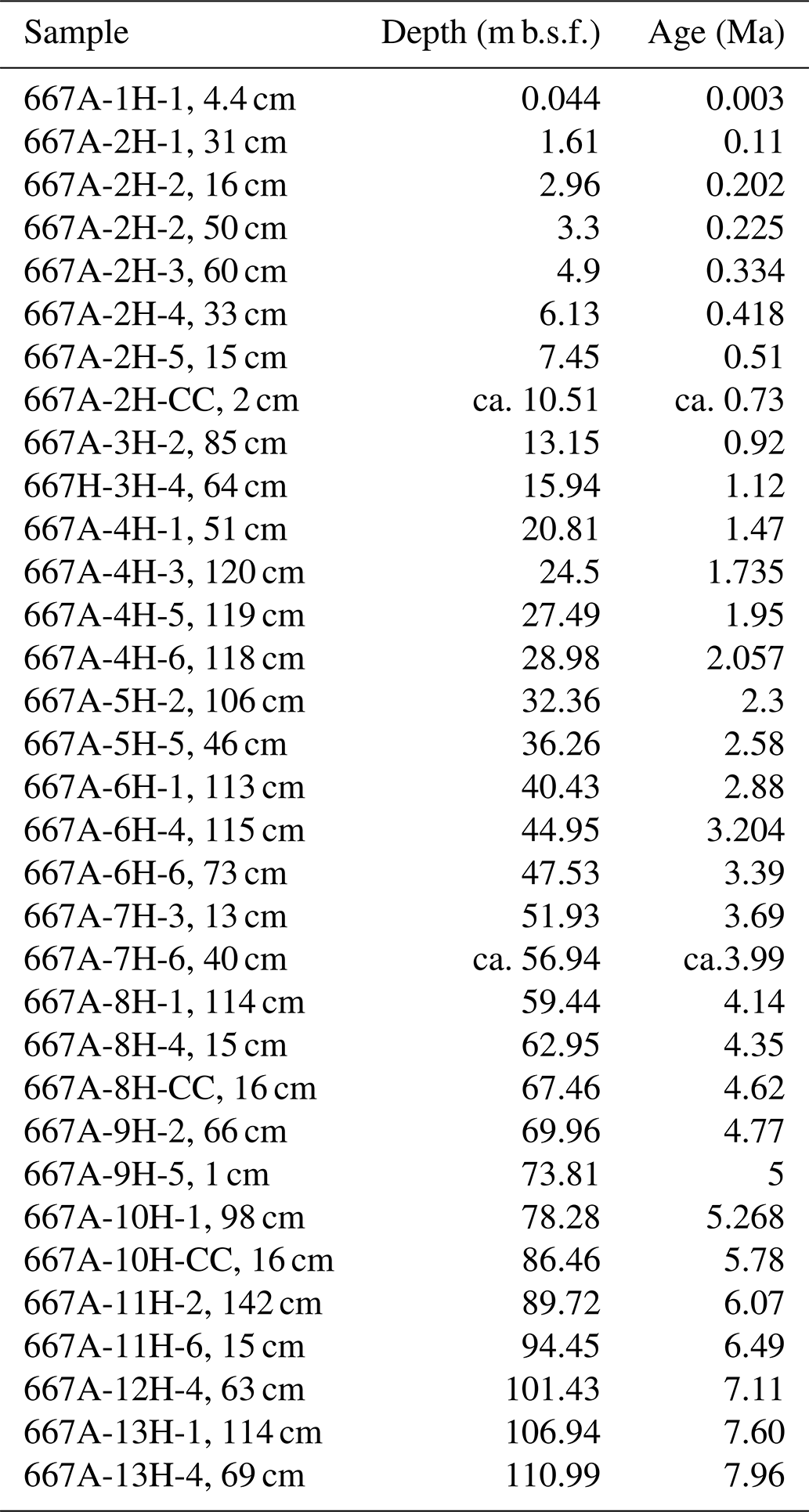
Due to the lack of stable isotopic data for this site, the age depth plot uses biostratigraphic data of PF and nannoplankton (Weaver and Raymo, 1989), as well as magnetostratigraphic events (Shipboard Scientific Party, 1988; Fig. 2). The Age Depth Plot programme by Lazarus (1992) was used to manually draw a line of correlation (loc) through recognised bio- and magnetostratigraphic events (Fig. 2). Using the loc's control points numerical ages were computed by linear interpolation with the help of the Age Maker (Lazarus, 1992) (NEPTUNE Age Model; see Supplement file “667A.loc95.txt”). The age depth plot is based on published core-depth information from Hole 667A (Shipboard Scientific Party, 1988) and biostratigraphic occurrences of first and last occurrence dates of nannofossils, planktonic and benthonic foraminifera, and magnetostratigraphic polarity reversals given in the initial reports and scientific results of that leg. The time chronology of Berggren et al. (1995) was applied to allow direct comparison to previous studies of Knappertsbusch (2007a, 2016).
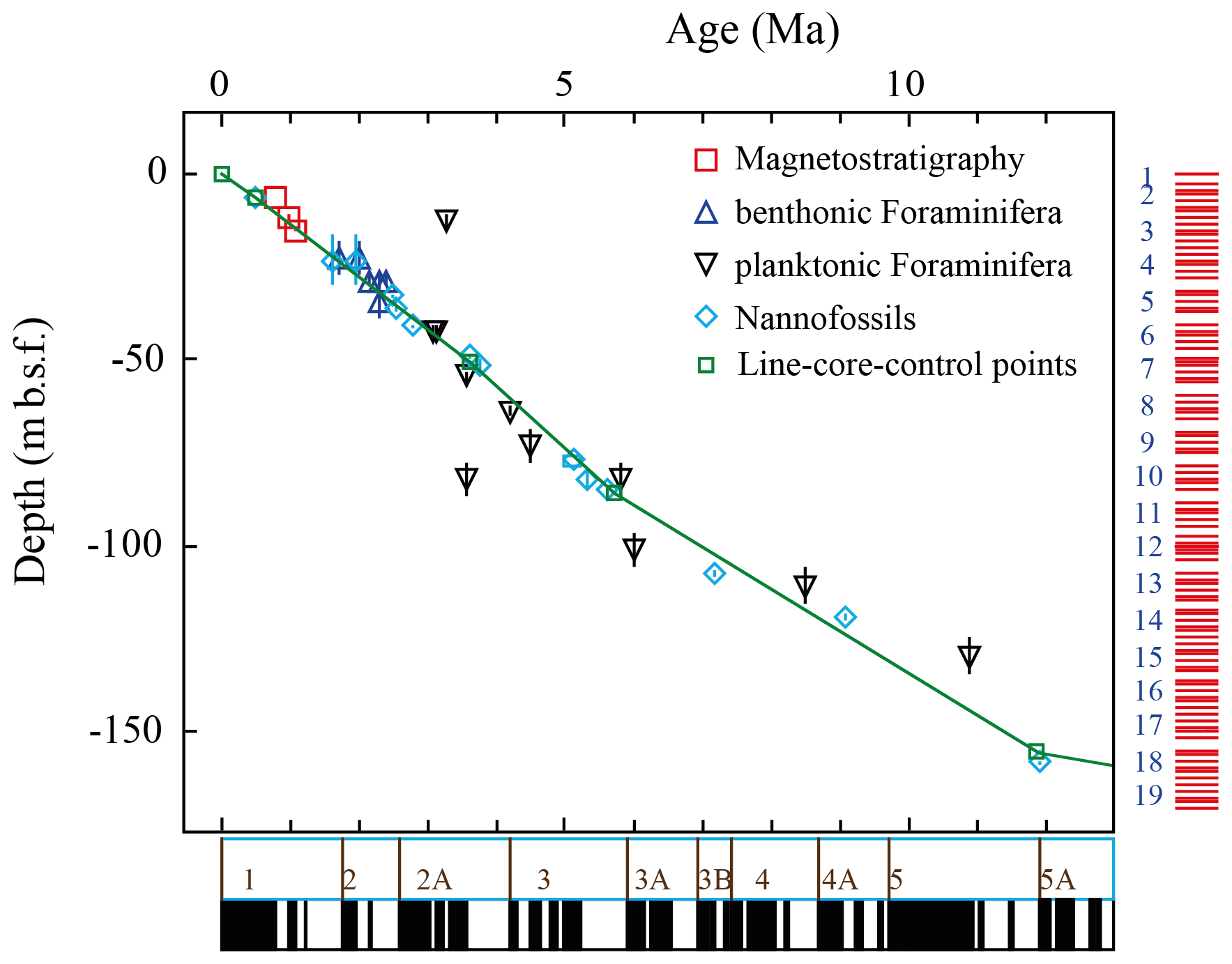
Figure 2Age (Ma) versus depth (m b.s.f. – metre below seafloor) plot for ODP Leg 108 Hole 667A, modified by Michael Knappertsbusch (personal communication, 2021). The green line represents the NEPTUNE Age Model. Biostratigraphic data were taken from Weaver et al. (1989) and from Weaver and Raymo (1989). Magnetostratigraphic data were taken from Shipboard Scientific Party (1988). The vertical bars within the symbols illustrate the depth range in which this event took place. The data for the palaeomagnetic reversals below the x axis are taken from Berggren et al. (1995). The red bars on the right side indicate cores and core recovery.
2.3 Sample preparation and parameter measurement
The procedure for the treatment of the samples follows that of Knappertsbusch (2016).
Approximately 2–3 cm3 bulk sediment per sample were dried at 40 ∘C over night and weighed. In a following step, the samples were gently boiled with water, containing soda as an additive, and wet-sieved with a 63 µm net. The fraction < 63 µm was decanted, dried and preserved. The > 63 µm fraction was dried at 40 ∘C for 24 h and weighed afterwards. A microsplitter was used to split the > 63 µm fraction until at least 200 menardiform specimens could be picked from the sample. This number of specimens was judged to be a reasonable compromise between efforts for picking and manual mounting, imaging, analytical and statistical steps, and the limited amount of time for this project. The specimens were mounted on standard faunal Plummer cells from P.A.S.I. (Prodotti e Apparecchiature Scienze e Industria) in keel view.
The preference was given to keel view because it allows a better orientation into (semi-)homologous positions than the umbilical or spiral views. In G. menardii's sister lineage, Globorotalia tumida, morphological variation in keel view has proven useful for the detection of evolutionary change (Malmgren et al., 1983). Intact specimens showing a menardiform morphology were picked from the sample splits. They include the whole G. menardii lineage, as well as members of the G. tumida lineage. In total, 4482 G. menardii, 764 G. limbata and 228 G. multicamerata specimens were picked from samples at 33 stratigraphic levels back to 8 Ma (Table 1). All study material is stored in the collections of the Natural History Museum Basel.
Digital images of the menardiforms were collected with the Automated Measurement System for Shell Morphology (AMOR), software version 3.28 (Knappertsbusch et al., 2009). This system automatically orientates and photographs tests in keel view to achieve orientation for outline analysis (Knappertsbusch et al., 2009). Repeated orientation tests with AMOR have shown that precision was 11.4 µm (3.2 % of mean radius of a specimen) when magnification was changing and 6.7 µm (1.9 % of mean radius of the test) at constant magnification (MorphCol supplement #29 by Knappertsbusch, June 2021). In addition, the programme “AutoIt” (Mary, 2013) was used for an automated processing of the imaging. The free software ImageJ 1.52i of the National Institute of Health was used to clean and pre-process images for outline coordinate extraction. Processing steps include removal of adhering particles, smoothing, enhancement of contrast, binarization and closing of single pixel embayments before storing the processed pictures as 640×480 pixel and 8 bit grey-level Tiff files. Adapted MorphCol software applications programmed in Fortran 77 from Absoft by Knappertsbusch (2007a, 2016) were used (Appendix Fig. A1) to extract cartesian outline coordinates and to derive morphometric measurements. These applications were converted to Fortran 95 versions and adapted for usage on Windows operating systems. The adapted MorphCol programmes and codes are deposited on the internal media server of the Natural History Museum Basel and will also be available on the PANGAEA repository.
These programmes considerably accelerate the process of measuring several different morphometric parameters from the images. Derived parameters include the spiral height (δX) and the axial length (δY), the aspect ratio (), the area of the specimen in keel view (Ar), the convexities of the spiral (A) and the umbilical (B) side, the ratio of the convexities (, the upper (Φ1) and the lower (Φ2) keel angles, the angle at the apex (Φ3), and the radii of the osculating circles in the upper (Rup) and the lower (Rlo) keel regions (see Fig. 3). This study focuses on the test-size parameter δX, δY and Ar. In order to compare specimens with dextral and sinistral coiling, dextral specimens were vertically mirrored using the adapted “DexFlip_win” programme, modified from Knappertsbusch (2016).
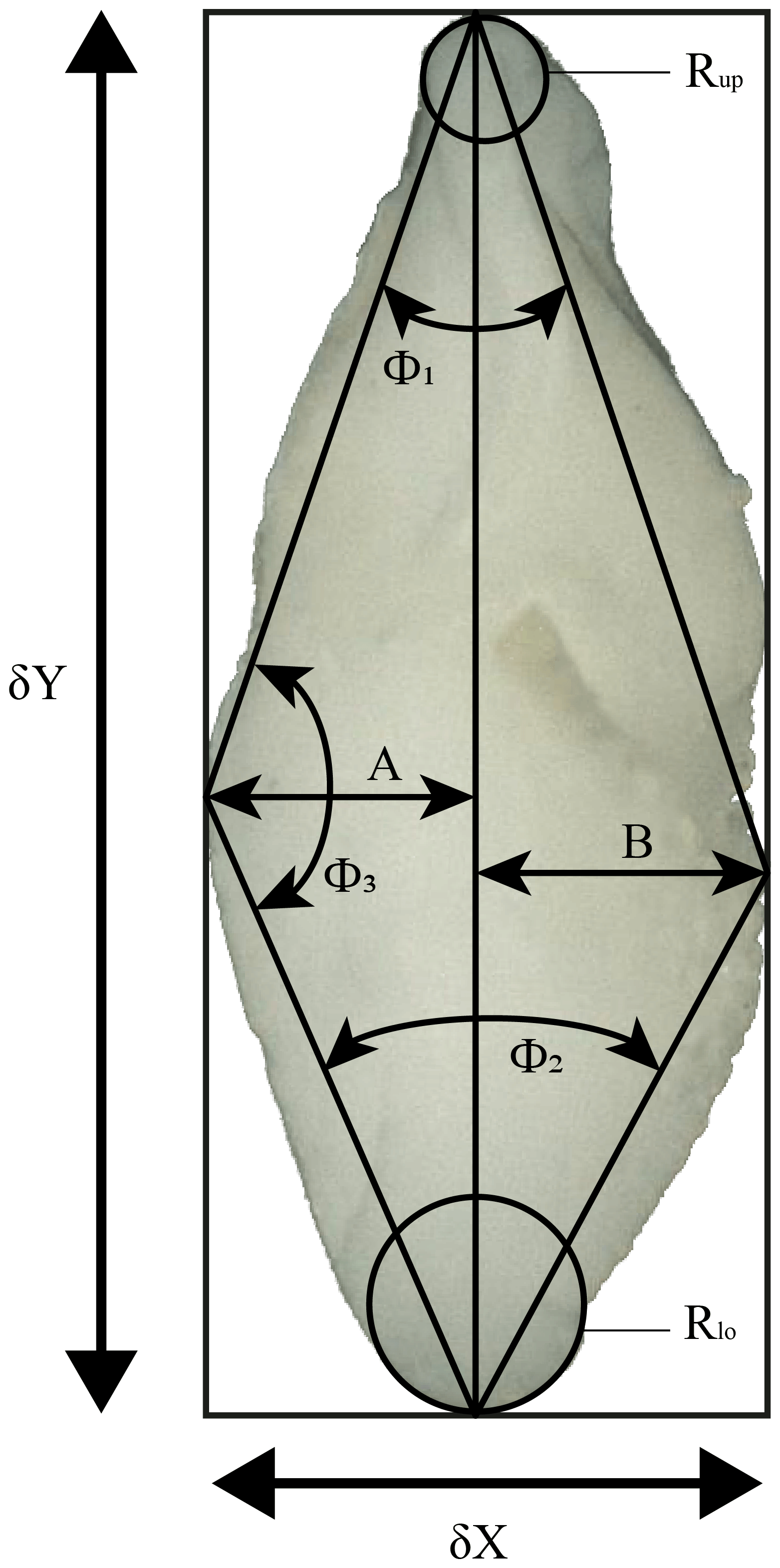
Figure 3Investigated morphometric parameters. δX: spiral height; δY: axial length; Φ1: upper keel angle; Φ2: lower keel angle; Φ3: angle at the apex; A: spiral convexity; B: umbilical convexity; Rup: radius of the osculating circle in upper keel region; Rlo: radius of the osculating circle in lower keel region.
2.4 Globorotalia menardii lineage–species discrimination
The identification on species level of picked menardiform specimens is based on illustrations in Kennett and Srinivasan (1983) and Bolli et al. (1985), as well as comparison with the reference collection to 49 Cenozoic planktonic foraminiferal zones and subzones prepared by Bolli in 1985–1987, which is deposited at the Natural History Museum Basel. This includes the species G. menardii, Globorotalia limbata, Globorotalia multicamerata, Globorotalia exilis, Globorotalia pertenuis, Globorotalia miocenica, Globorotalia pseudomiocenica, Globorotalia tumida, Globorotalia merotumida, Globorotalia plesiotumida and Globorotalia ungulata. Diagnostic features included the size, the outer wall structure (shiny surface due to finer perforation), number of chambers in the last whorl, and the δX and δY ratio. After species determination, forms like G. exilis, G. pertenuis, G. miocenica, G. pseudomiocenica and the G. tumida group, as well as the G. menardii subspecies G. m. cultrata, G. m. fimbriata, G. m. gibberula and G. m. neoflexuosa, were sorted out and not included in the present morphometric study. Thus, the dataset presented herein only contains specimens of G. menardii menardii (in the following referred to as G. menardii), G. limbata and G. multicamerata.
Globorotalia menardii is discriminated from its extinct descendants G. limbata and G. multicamerata by the number of chambers in the last whorl (Fig. 4). This pragmatic approach was applied because the apparently most distinctive morphological character of G. limbata, its limbation of the chamber sutures on the spiral side (Kennett and Srinivasan, 1983), is difficult to recognise and is also observed in G. menardii and G. multicamerata (Knappertsbusch, personal communication; personal observation). In order to solidify a possible cladogenetic pattern between G. menardii and G. limbata, the present study experimented with the pragmatic discrimination that G. limbata, which became extinct during the early Pleistocene at 2.39 Ma (Wade et al., 2011), has only seven chambers in its last whorl. Menardiform specimens with six or fewer chambers were determined as G. menardii. Globorotalia multicamerata has more than seven chambers in its last whorl and became extinct in the Pliocene at 3.09 Ma (Berggren et al., 1995).

Figure 4The investigated species in spiral, umbilical and keel view. 1–3: Globorotalia menardii, typically found during the past 2 Myr in the Atlantic Ocean, sample 667A-1H-1, 3–4 cm, specimen 667011004aK2501. 4–6: Globorotalia menardii, preferentially found in samples older than 2 Ma, sample 667A-6H-4, 113–114 cm, specimen 667064114bK0301. 7–9: Globorotalia limbata, sample 667A-6H-4, 113–114 cm, specimen 667064114aK5701. 10-12: Globorotalia multicamerata, sample 667A-6H-4, 113–114 cm, specimen 667064114aK5201. Scale bar: 100 µm. Images were produced with Keyence VHX-6000 microscope.
Knappertsbusch (2016) refers to the disappearance of G. limbata as a possible pseudoextinction because of the sporadic occurrence of specimens of menardiforms with seven chambers in the last whorl after 2.39 Ma.
2.5 Univariate and contoured frequency diagrams
Statistical analysis and univariate parameter-versus-age plots were prepared with RStudio (V. 3.5.3; RStudio Team, 2020), using the packages psych (Revelle, 2018), readxl (Wickham and Bryan, 2019), ggplot2 (Wickham, 2016), pacman (Rinker and Kurkiewicz, 2018) and rio (Chan et al., 2018). For the generation of contour frequency diagrams (CFDs) the commercial software applications Origin 2018 and Origin 2019 by OriginLab Corporation were used. CFDs per species help to detect shifts in the dominant test size of populations throughout time. The same method was applied in Knappertsbusch (2007a, 2016) and enables a direct comparison of evolutionary change in Hole 667A with previous studies. Emergence and divergence of new frequency peaks between subsequent samples may help to empirically identify signs of cladogenetic splitting or anagenetic evolution in the lineage of G. menardii–G. limbata–G. multicamerata. The CFDs were constructed from so-called “gridded files” obtained by plotting δX versus δY, superposing a grid with grid-cell sizes of ΔX = 50 µm and ΔY = 100 µm (see Knappertsbusch, 2007a, 2016) and then counting the number of specimens per grid cell. This gridding procedure was performed with the programme “Grid2.2_win” (adapted MorphCol software by Knappertsbsuch, 2007, 2016), and the result was a two-dimensional matrix of absolute frequencies of specimens per grid cell. No smoothing of frequencies was applied because experiments revealed an increasing loss of frequency variation with increasing size of bin width. However, in contrast to Knappertsbusch and Mary (2012) and Knappertsbusch (2016), local absolute specimen frequencies were used throughout instead of relative frequencies.
Different contour intervals were used for the CFDs because the number of G. menardii specimens per sample varies from 1 (667A-5H-2, 105–106 cm) to 273 (667A-4H-3, 120–121 cm). This approach increases the legibility of the single CFDs because setting a high contour interval in a sample with few specimens would have levelled out the CFD. Conversely, choosing a low contour interval would lead to exaggerated contour line densities in CFDs when the number of specimens is high.
2.6 Volume density diagrams
Volume density diagrams (VDDs) were made with the commercial software Voxler 4 by Golden Software. This method was shown to be useful to illustrate and visualise evolutionary tendencies in coccolithophores but also in menardiform globorotallids (Knappertsbusch and Mary, 2012). Conceptually, they are constructed by stacking the contour frequency diagrams from different time levels. In this way, the grid cells of plane bivariate contour frequency diagrams expand to include time as the third dimension, e.g. spiral height, axial length and time. The local frequency is the fourth dimension (F). In this manner, a four-dimensional unit (X, Y, time, F) called “voxel” is generated. The component F of a voxel (local frequency) can then be represented as the iso-surface, which is done using Voxler. In other words, the iso-surface of the VDD represents the distribution of a constant local frequency through time (Knappertsbusch, 2016). High iso-values form the core of a VDD and represent abundant specimens. They allow the main evolutionary path through time to be investigated. Low iso-values illustrate rare specimens and show the extremes of test size. They are often related to innovation caused by evolution or represent extreme forms introduced by dispersal.
The protocol for constructing a VDD developed by Knappertsbusch (2007a, 2016) and Knappertsbusch and Mary (2012) was modified to improve the level of coincidence between the plane CFDs and VDDs. The most important changes concern (1) the usage of absolute instead of normalised frequencies in the input files, (2) a different set-up in the gridder option and (3) the modification of the iso-value. A detailed list of the adjustments used is given in the Supplement (File “VDD_set-ups.txt”).
The commercial software PDF3D ReportGen by Visual Technology Services Ltd was used to create the three-dimensional model from the Open Inventor (.iv) file format of a VDD when exported from Voxler.
In a first step of analysis, the test-size evolution of G. menardii at Hole 667A was investigated by plotting δX and δY versus the age. This is the simplest analysis for evolutionary change and allows a direct comparison with previous data from Knappertsbusch (2007a, 2016). At Hole 667A, this test-size variation shows different phases of evolution through time: these two parameters serve as a primary measure for the intraspecific variability in the G. menardii lineage.
3.1 Morphological parameters through time
The comparison of the test size of G. menardii during times of co-occurrence with its sister taxa G. limbata and G. multicamerata and the size after the extinction of G. limbata and G. multicamerata may give evidence about possible shifts in the ecology of G. menardii. Major changes in the size of G. menardii before and after the extinction of its sister taxa probably point to an adaption to a different, new niche, e.g. in terms of “incumbency replacement” (Rosenzweig and McCord, 1991). Between 7.96 and 2.58 Ma, the evolution of δX in G. menardii shows three peaks at 7.11, 5.78 and 3.99 Ma in the mean and median values (Fig. 5). Except for the sample 667A-10H-1, 97–98 cm at 5.26 Ma, at which the maximum size of G. menardii does not decrease as the mean and median do, the maxima of δX follow the trends of the corresponding mean and median values. The maximum values exhibit one peak at 7.11 Ma and two “peak plateaus” from 5.78 to 5.26 Ma and 4.35 to 3.69 Ma. In samples from 2.3 Ma and younger, δX of G. menardii increases to a maximum value of 619 µm in the youngest sample (667A-1H-1, 3–4 cm; 0.003 Ma), which is almost a doubling of the size reached between 7.96 and 2.58 Ma (maximum value 365 µm at 3.69 Ma). Prior to its extinction, G. limbata shows similar maximum (Fig. 5b) and mean δX peaks (Fig. 5d) as G. menardii at 7.11, 5.78 and 4.14 Ma. On average, populations of G. limbata are slightly larger in size than those of G. menardii. Specimens with seven chambers in the last whorl, which are considered as G. limbata, still occur after 2.58 Ma but only sporadically and in low numbers, and no statistically significant statements are possible for those times.
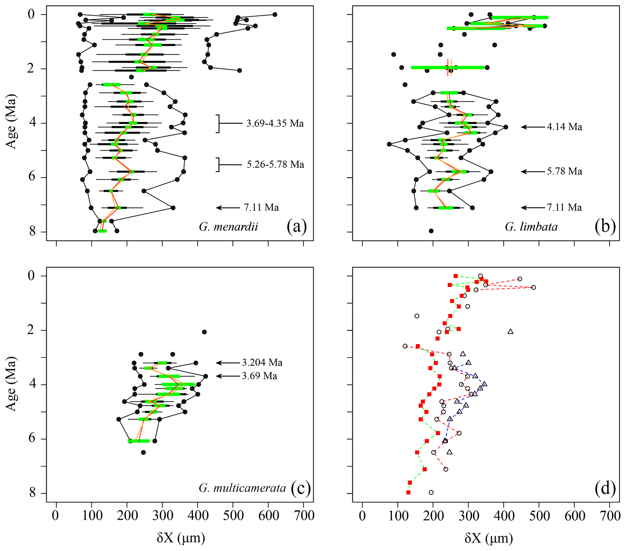
Figure 5Spiral height (δX) in keel view (in µm) versus time (Ma) at ODP Hole 667A for (a) G. menardii, (b) G. limbata, (c) G. multicamerata and (d) the mean values of the three species. In (a)–(c), black dots represent minimum and maximum values. The thin horizontal black bars represent the 10 % to 90 % sample percentiles and thick black bar bars the lower and the upper quartiles, and the green horizontal bar shows the confidence interval of the mean. Means are illustrated as a vertical red line and median values by an vertical orange line. In (d), δX means of G. menardii are shown as red squares, those of G. limbata by black circles and means of G. multicamerata by black triangles. Samples containing fewer than three specimens of the corresponding species are shown as isolated symbols because this number does not allow reasonable statistical analysis.
Globorotalia multicamerata attains the largest size of the three species at times before 3 Ma (Fig. 5c). It surpasses G. menardii and G. limbata in test-size mean and maximum values in all samples in which it occurs (Fig. 5d). Exceptions are the samples at 6.07 Ma, which have the same mean value as G. limbata, and at 2.057 Ma. No specimen was found at 5.78 Ma. Thus, G. multicamerata only exhibit one major peak in the maximum values at 3.69 Ma and in the mean values at 3.99 Ma.
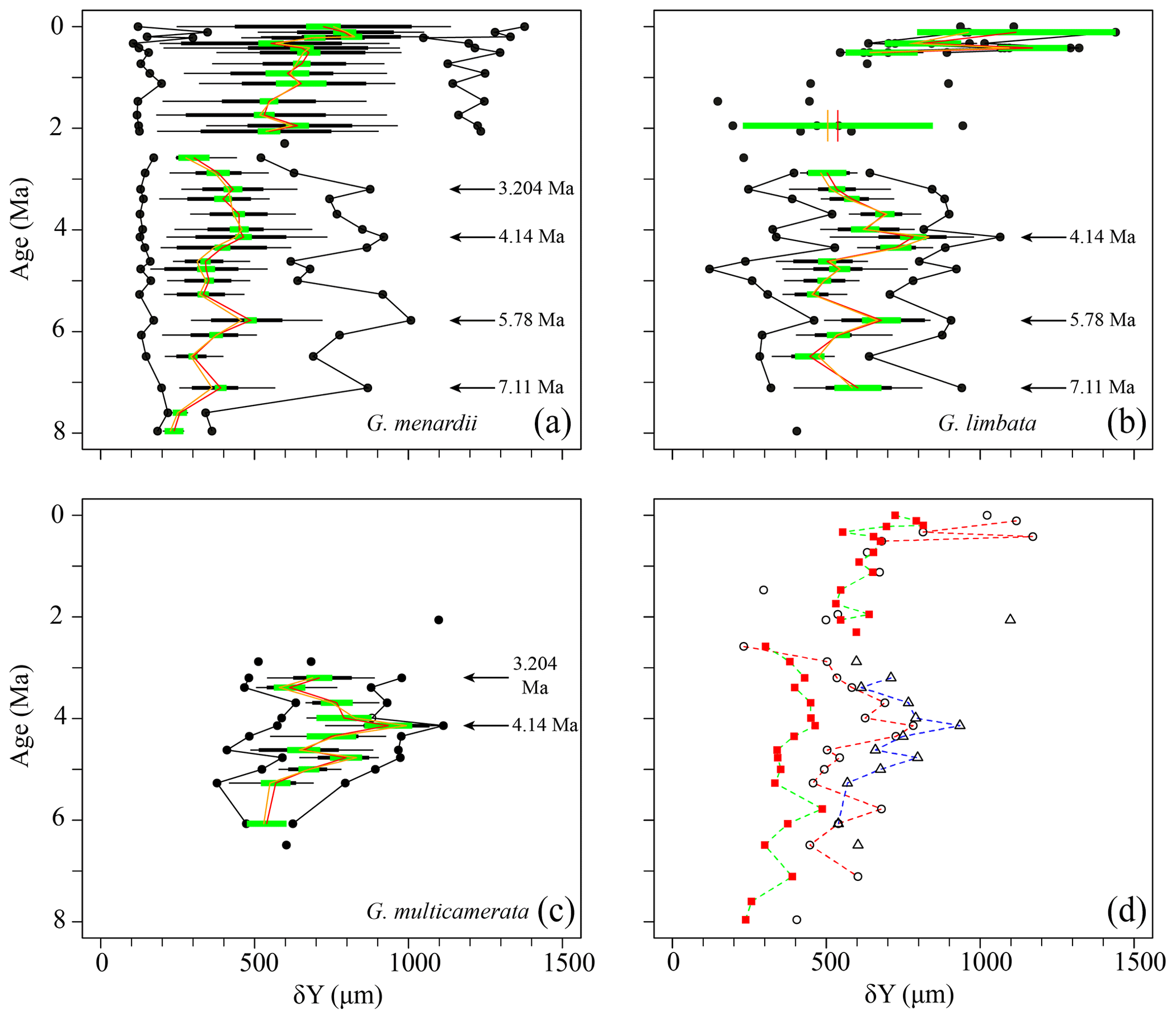
Figure 6Axial length (δY) in keel view (in µm) versus time (Ma) at ODP Hole 667A for (a) G. menardii, (b) G. limbata, (c) G. multicamerata and (d) the mean values of the three species. See Fig. 5 for the explanation of the symbols.
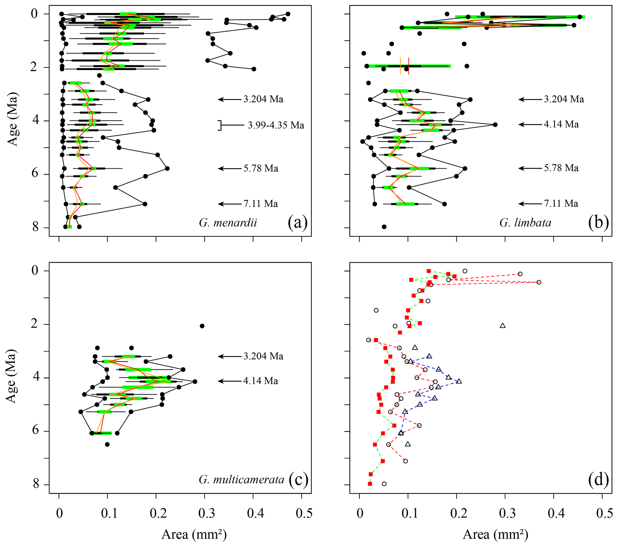
Figure 7Test area (Ar) in keel view (in mm2 ) versus time (Ma) at ODP Hole 667A for (a) G. menardii, (b) G. limbata, (c) G. multicamerata and (d) the mean values of the three species. See Fig. 5 for the explanation of the symbols.
Similar to δX, the mean and median values of δY also show three major peaks (7.11, 5.78, 4.14 Ma) for G. menardii and G. limbata between 7.96 and 2.58 Ma (Figs. 6, 7). Maxima of δY exhibit similar peaks, but note a fourth peak in δY at 3.204 Ma for G. menardii (Fig. 6a).
Measurements of Ar are shown in Fig. 7. Between 7.96 and 2.58 Ma the Ar of G. menardii reveals three peaks at 7.11, 5.78 and 3.204 Ma and a plateau from 4.35 to 3.99 Ma. The data also show a peak in Ar for G. limbata at 4.14 Ma. Between 2.58 and 2.057 Ma, the maximum values of δY (Fig. 6a) of G. menardii more than double from 520 µm to 1235 µm, while Ar increases 5-fold from ca. 0.08 to 0.4 mm2 (Fig. 7).
For G. multicamerata, the maximum and mean δY and Ar values show a similar pattern as δX (Figs. 6c, 7c) but with a major peak at 4.14 Ma. This species exhibits the largest size in these two parameters in comparison to the other two species.
The three parameters show a high degree of overlap between the three species. However, morphological overlap between these species point to strong interspecific size variation. Globorotalia multicamerata exhibited the largest mean population test size and G. menardii the smallest mean size, while G. limbata was intermediate.
3.2 Contour frequency diagrams of spiral height and axial length
As already mentioned in the “Materials and methods” section (Sect. 2.5), CFDs may help to detect patterns of cladogenetic splitting or anagenetic evolution by identifying shifts in the dominant test size of populations through time. The underlying grid-cell size for CFDs (and VDDs in the next section) is 50 µm in δX direction and 100 µm in δY direction.
In general, the contour frequency plots of G. menardii (Fig. 8) show that size measurements vary almost linearly by a diagonal semi-continuous morphocline in the δX and δY morphospace. This trend is due to a flattening of the test during the ontogenetic growth of the individuals (Caromel et al., 2016). As was already recognised in the univariate parameter-versus-time diagrams, two different phases of shell size development can be distinguished in the CFDs. The first phase ranges from 7.96 Ma until about 2.88 Ma and is characterised by populations with a dominant test size smaller than 300 µm in δX and smaller than 600 µm for δY for G. menardii, as well as predominantly unimodal distributions of the population size (Fig. 8). The only sample in this first phase showing bimodality is at 4.35 Ma. At 2.58 and 2.3 Ma, the G. menardii population is very reduced and small or almost completely vanished. A different pattern appeared from 2 Ma until the present. In that younger interval, several samples exhibit visually distinct bimodal distributions along the δX versus δY morphocline (2.057, 1.95, 1.735, 1.12, 0.92, 0.418, 0.334, 0.11 and 0.003 Ma). The smaller mode is limited to a range of 200 µm (δX) and 300 µm (δY), while the larger surpasses 250 µm (δX) and 600 µm (δY) in each case. There is a noteworthy change in the youngest sample (0.003 Ma), where the majority of specimens occur above the diagonal separation line (see Fig. 8), while specimens of older samples are mostly distributed below that line. This is also visible in the VDD in Sect. 3.4.
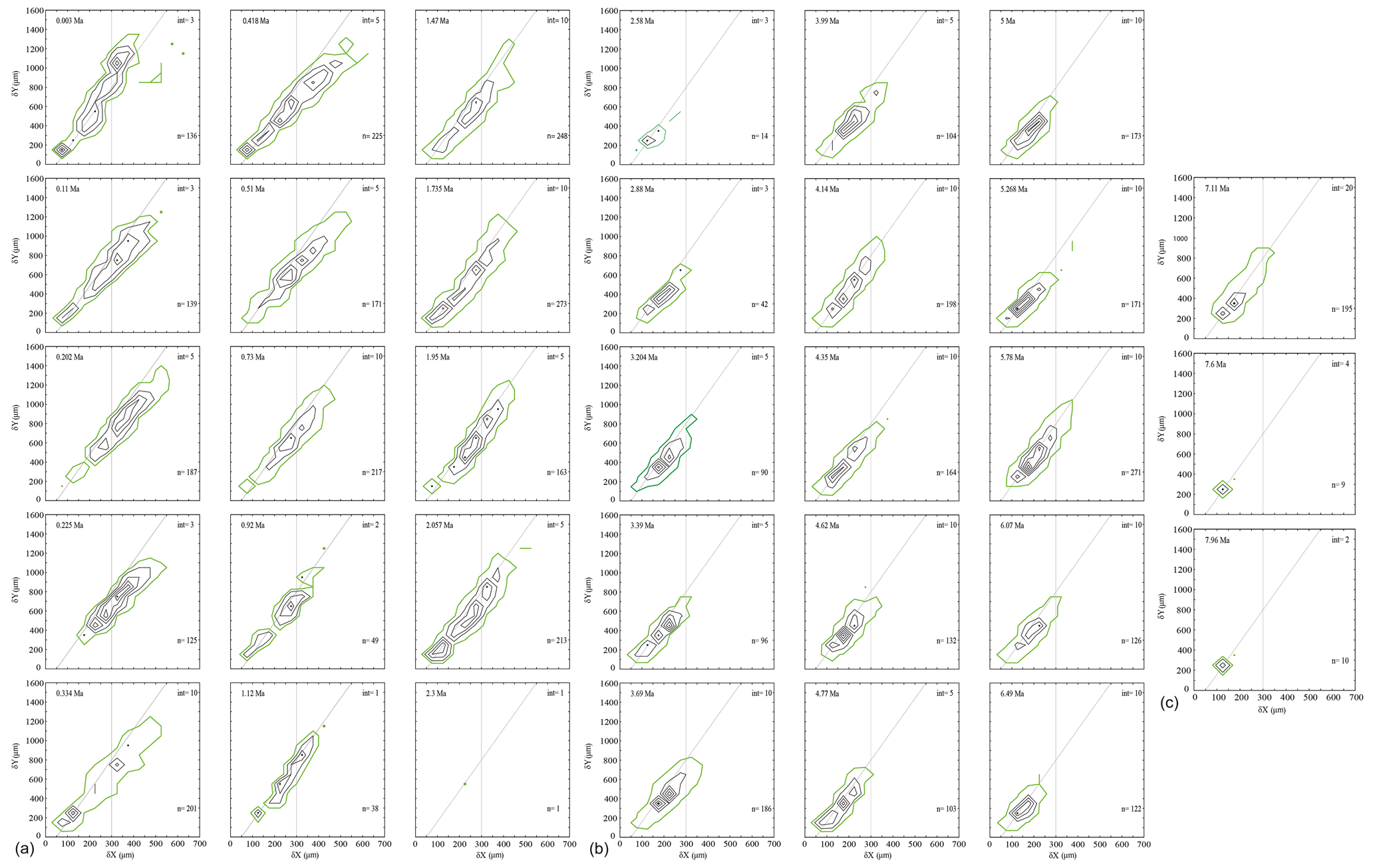
Figure 8(a, b, c) Contoured frequency plots of spiral height (δX) on the x axis versus the axial length (δY) on the y axis of Globorotalia menardii in keel view at ODP 108 Site 667 from 0.003 to 7.96 Ma. The upper-left corner shows the age (Ma). “int” indicates the contour interval in the number of specimens per grid cell. The grid-cell size is 50 µm × 100 µm in direction of δX and δY, respectively. “n” in the lower-right corner gives the number of specimens represented in the diagram. Green-coloured contour lines and dots represent the contour interval from 0 to 1. The diagonal grey line is drawn to separate the morphotype of G. menardii menardii (area below the line) and G. menardii cultrata (area above of the line) proposed by Knappertsbusch (2007a). The vertical grey line at δX = 300 µm delimits the dominant population of G. menardii older than 2.88 Ma and is also drawn for comparison.
3.3 Bimodal patterns in contour frequency diagrams
Several samples younger than 2.057 Ma (2.057, 1.95, 1.735, 1.12, 0.92, 0.418, 0.334, 0.11 and 0.003 Ma) and the sample from 4.35 Ma visually display a bimodal distribution, in which the peaks are separated either at ca. δX = 200 µm or at δX = 300 µm (Fig. 8). If the described bimodality patterns were to indicate speciation within G. menardii, modal centres would connect into continuous branches that diverge for the last 2 Myr. Populations can be more closely inspected through vertical stacking of CFDs via a volume density diagram (see Sect. 3.4).
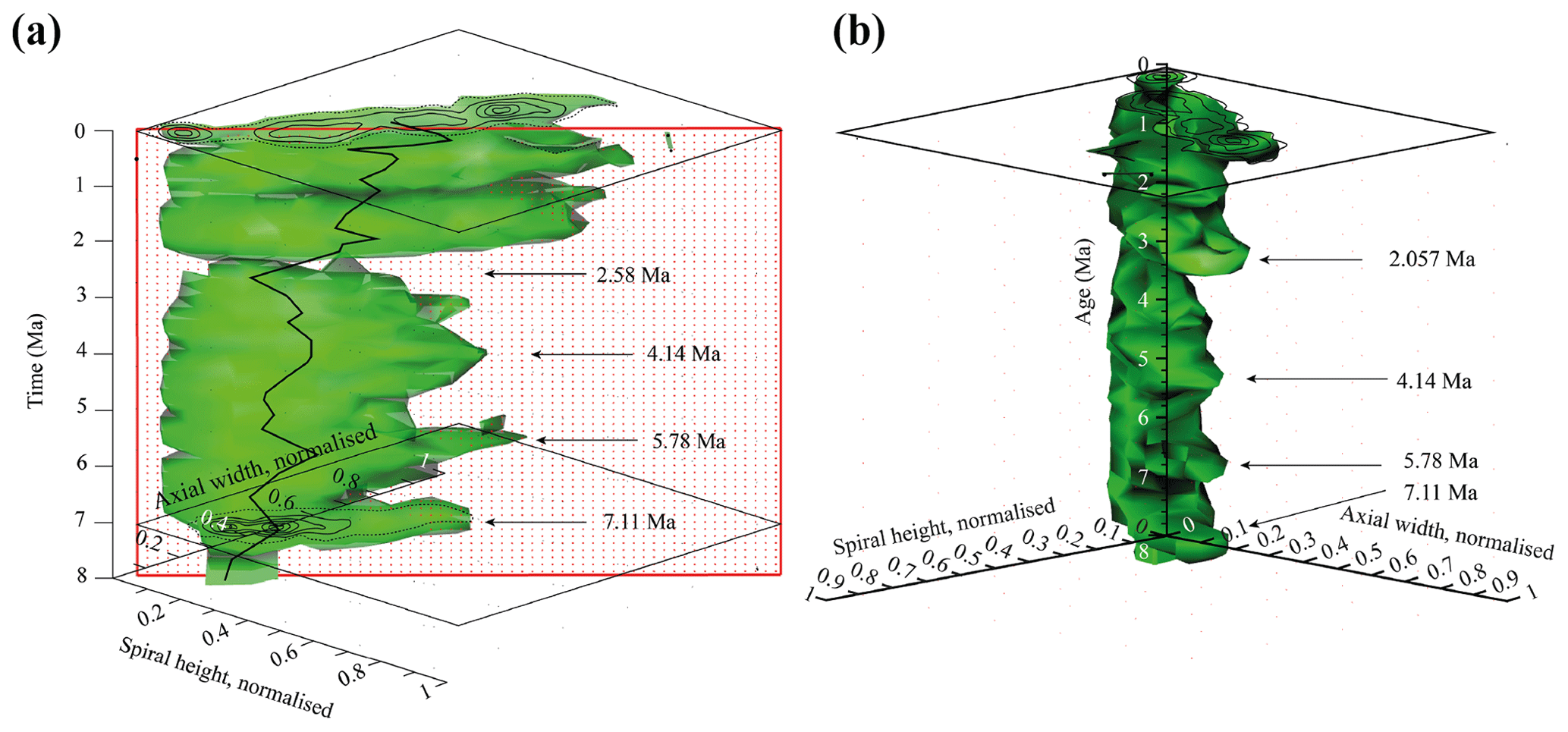
Figure 9Volume density diagrams (VDD) of the normalised spiral height (δX) versus the normalised axial width (δY) over the past 8 Myr for G. menardii at the eastern tropical Atlantic Hole 667A. The shown iso-surface has a value of 0.89447168, which equals the frequency of one specimen. Thus, it represents rare, innovative specimens. (a) VDD in side view. The red, dotted plain represents the section shown in Fig. 10. The CFDs of the samples from 0.003 and 7.11 Ma are displayed. The black line represents the mean values. (b) VDD in front view. The CFD of the sample from 0.003 Ma is displayed as an example. The arrows at 7.11, 5.78 and 4.14 Ma point to size peaks, and the arrow at 2.58 Ma marks the sample with the smallest observed test size. The settings for the VDD construction are given in the Supplement (file “VDD_set-up_data.txt”).
3.4 Volume density diagrams
The iso-surface of Fig. 9 illustrates the test size of rare, often innovative specimens, which either evolved within the Atlantic Ocean or intruded by dispersal. As the VDD is basically a stacking of the individual CFDs, it shows the same peaks at 7.11, 5.78 and 4.14 Ma for G. menardii. The VDD clearly illustrates the size decrease during the interval from 4.14 Ma until 2.58 Ma and the striking size increase from 2.58 to 2.057 Ma (Fig. 9a). The size reached at 2.057 Ma is unprecedented.
Of special note is the aberrant steeper slope of the youngest CFD (0.003 Ma; Fig. 8), which is displayed with respect to the rest of the VDD towards elongated and flattened specimens. Such a trend to flat specimens was also observed in the uppermost Quaternary of DSDP Site 502 (Knappertsbusch, 2007a). In the present case specimens have developed a strong keel and so are presumably not classified as G. m. cultrata.
An interactive version of the VDD can be found in the three-dimensional PDF file “VDD_3D_PDF.pdf” (see Supplement).

Figure 10(a) Longitudinal section (offset value = 0) through the 45∘ view on the volume density diagram of Hole 667A in a palaeoceanographic context. The dotted line represents a density of one specimen per grid cell, and solid lines are contours at density intervals of five specimens per grid cell. The evolution of mean values through time is shown as a thick black line. (1) The time interval in which a shift to increased amplitude of glacial–interglacial cycles and a corresponding 100 Kyr fluctuation in ice sheets is observed (Clemens et al., 1996; Ivanova, 2009). (2) The cooling trend, which leads into the NHG (Chapman, 2000). (3) The mid-Pliocene warm period (mPWP; Haywood et al., 2016). (4) The time interval in which the final closure of the Central American Seaway (CAS) is supposed by Bartoli et al. (2005), Jackson and O'Dea (2013), and O'Dea et al. (2016). (5) The time interval of the Mediterranean salinity crisis (Krijgsman et al., 1999). (6) The intensification of the Late Miocene Antarctic Glaciation (ILMAG) (Chaisson and Ravelo, 1997). (b) The right side shows εNd isotopic curve at Site 1088 in the South Atlantic taken from Dausmann et al. (2017), a proxy for the AMOC strength. The black line with circles represents the original data from Dausmann et al. (2017) and the red line a smoothed version, produced with the RStudios' command “smooth.spline” at the value of 0.35. (c) The black triangles on the left side display the investigated samples. The boxes on the right side show the time intervals in which the giant G. menardii specimens occurred at Sites 667, 925 and 502 and in which the size increase is presumed to have taken place. The arrows show the first appearance date (FAD) of giant G. menardii specimens and the last appearance date (LAD; more than one specimen per sample split) of G. limbata and G. multicamerata at Site 667.
3.5 Longitudinal section of frequencies of spiral height and axial length through time
A longitudinal section through the VDD, as shown in Fig. 10, allows us to check for and identify changes and shifts in the frequencies and to investigate whether modal centres in size distribution arrange along continuous and diverging branches through time. The occurrence of multiple, distinct density peaks in the CFD may indicate the occurrence of populations with different test sizes. If these density peaks combine to continuous morphological clades through time, diverging branches may point to morphological speciation within G. menardii. A clear split into robust branches that separate through time cannot be recognised in Fig. 10. During the time interval from 7.96 to 2.58 Ma, one continuous clade consisting of two or more modes can be identified, which follows the mean value. Higher up in the core, a tendency to a bifurcation into two distinct clades is indicated around 1.735 Ma. This sample was already mentioned to develop bimodality in CFDs (Fig. 8). In the youngest part of the core this bifurcation is no longer observed despite the presence of distinct modal centres in individual CFDs, during which G. menardii tends to gradually increase its test size. The complexity of the size evolution of G. menardii through time is further illustrated in two parallel sections in 45∘ orientation with different offsets and three orthogonal sections at 135∘ (Appendix Figs. A2–A7). The different perspectives of the VDD show other density peak trends. An “ideal” description of maximal evolutionary trends would require a flexural vertical section plain at 45∘.
Figure 10 indicates that the test-size evolution may be directly or indirectly affected by major palaeoceanographic events. The overall decrease from ca. 4 to 2.5 Ma follows the closure of the Isthmus of Panama and the intensification of the NHG. The figure also indicates a potential influence of the AMOC strength on the test size (see Sect. 4.1.3).

Figure 11Percentage of sinistral specimens within the G. menardii population through time. (a) Tropical Atlantic Ocean Site 667 (green; this study), 502 (blue; Knappertsbusch, 2007b) and 925 (orange; Knappertsbusch, 2015). (b) Eastern tropical Pacific Ocean Site 503 (Knappertsbusch, 2007c). The grey areas represent the recognised phases as mentioned in the text. The lighter grey bar from 5.3 Ma until ca. 4 Ma shows the extended phase 1 for Sites 502, 503 and 925.
3.6 Changes in coiling direction in G. menardii
The data also show changes in the coiling direction of G. menardii, which may be related to understand evolutionary changes (see, for example, Bolli, 1950).
In the ETAO, three different phases in the predominant coiling direction of G. menardii were observed, in which patterns in the predominant coiling direction change (Fig. 11a). In the first phase from 7.96 until 5.268 Ma, coiling seems to frequently swing between sinistral and dextral. During the second phase from 5.268 to 2.057 Ma dextrally coiled specimens dominated (> 90 %, except at 2.58 Ma with 78.5 %). In the youngest phase, lasting from 2.057 Ma to present, sinistral coiling prevailed strongly (> 95 %). These phase are in agreement with Bolli and Saunders (1985) and references therein (Bolli, 1950; Bermúdez and Bolli, 1969; Robinson, 1969; Bolli, 1970; Lamb and Beard, 1972; Bolli and Premoli Silva, 1973). It is interesting that sites from the WTAO (925B), the Caribbean Sea (502) and the eastern tropical Pacific Ocean (503) exhibit a similar history of changes in the coiling direction in menardiforms (Fig. 11), although phase 1 extends at these sites until ca. 4.15 Ma, and the stratigraphic resolution for trans-oceanic correlation remains rather low.
Nevertheless, the reversal in the preferential coiling direction from dextral (phase 2) to sinistral (phase 3) at ca. 2 Ma is nearly synchronous at all of the above-mentioned sites and coincides with the stratigraphic entry of giant G. menardii forms in the Atlantic Ocean.
4.1 Size variation in Globorotalia menardii
A substantial test-size increase in G. menardii is observed at Hole 667A. Within the short time interval from 2.58 to 2.057 Ma, the size more than doubles (Figs. 5, 6, 7, 8). Knappertsbusch (2007a, 2016) observed a similar expansion in test-size evolution in western Atlantic ODP Hole 925B and at the Caribbean Sea DSDP Site 502 between 2.58 and 1.95 and 1.7 Ma, respectively. He considered two hypotheses which could explain this observation: a rapid faunal immigration via Agulhas leakage or rapid evolutionary test-size increase by punctuated evolution.
The new data from Hole 667A are discussed in the context of these two hypotheses. Although the results of this site cannot prove or reject one of the hypotheses, they may reveal evidence for their likelihood. A third hypothesis is introduced which proposes the AMOC strength as a possible (palae-)oceanographic influencer on the test size of G. menardii and could explain the size evolution during the time interval from 8 to ca. 2 Ma.
4.1.1 Agulhas leakage hypothesis
In the Agulhas leakage hypothesis, G. menardii is assumed to have been entrained from the subtropical Indian Ocean into the tropical Atlantic Ocean by episodic and especially strong Agulhas faunal leakage events (Knappertsbusch, 2016).
The Agulhas leakage is known to disperse Indian Ocean biota into the Atlantic Ocean on a large scale via giant eddies (Peeters et al., 2004; Caley et al., 2012; André et al., 2013; Villar et al., 2015). These eddies form when water masses of the Agulhas Current separate from the retroflection point off South Africa (e.g. Lutjeharms and Van Ballegooyen, 1988; Norris, 1999; Bard and Rickaby, 2009; Biastoch et al., 2009; Beal et al., 2011; Fig. 1). At ODP Site 1087, which is located in the southern Benguela region, the Agulhas leakage has been found to exist since 1.3 Ma by presence and absence of G. menardii (Caley et al., 2012).
Globorotalia menardii is a well-known tropical dweller (Caley et al., 2012; Schiebel and Hemleben, 2017, and references therein). Over the southern tip of Africa, the tropical provinces of the Atlantic and Indian oceans are disconnected by strong fronts from the transitional province of the Southern Ocean. These frontal barriers are rather difficult to surpass for tropical species like G. menardii and so prevent continuous genetical exchange. The Agulhas leakage mechanism and its probable changes in strength and intensity allow tropical plankton faunas to surmount oceanographic barriers and to transport them from the tropical Indian Ocean into the southern Atlantic and further into the tropical Atlantic (Caley et al., 2012). The relatively sudden appearance of giant G. menardii in the Atlantic Ocean might thus be explained by such a large distance dispersal of tropical populations at a time when the Agulhas leakage became possibly intensified between ca. 2.58 and 2.057 Ma. If true, this would pre-date the existence of the Agulhas leakage by at least 0.7 Myr.
Interestingly, giant menardiforms occurred ca. 0.1 Myr earlier at the ETAO Site 667 than at the WTAO Site 925. Under present oceanographic conditions, simulations showed that Agulhas rings follow predominantly the South Equatorial Current rather than the Benguela Current along the southwest African continent (Biastoch et al., 2009; van Sebille et al., 2011; Rühs et al., 2013; Laxenaire et al., 2018; Fig. 1). With this scenario in mind, one would expect the giant forms to first be transported into the WTAO, which on first sight would contradict the Agulhas hypothesis. However, an eastward meandering and fluctuation in strength of the Agulhas leakage ring pathway during different climatic conditions than today could explain the observed pattern. Instead of traversing the South Atlantic, rings may have drifted closer to the coast of southwest Africa. In such a scenario, the giant G. menardii type dispersing from in the Indian Ocean would have reached the ETAO first.
An alternative idea is proposed by Norris (1999), according to which unfavourable environmental conditions in the WTAO prevented G. menardii from stabilising viable populations, which could explain the size differences during 2.58–1.95 Ma at Hole 925B. The Indian-Ocean-influenced water masses were perhaps further transported to the ETAO via the North Equatorial Countercurrent (Fig. 1), where more favourable conditions prevailed, allowing G. menardii to thrive. A similar hypothesis of presence and absence of suitable environmental conditions was already considered to explain a distinct short pulse of Globorotalia truncatulinoides in the southern Atlantic Ocean at 2.54 Ma (Spencer-Cervato and Thierstein, 1997; Sexton and Norris, 2008).
According to Chaisson and Ravelo (1997), a trade-wind see-saw between the ETAO and the WTAO prevailed, which possibly resulted in unfavourable environmental conditions for G. menardii at Site 925B between 2.5 and 1.95 Ma. These authors argue that trade winds influence the thermocline depth at each side of the equatorial Atlantic Ocean in a reverse way: increased trade winds in the WTAO pile up warm surface waters, leading to a massive thermocline layer and a deeper thermocline. At the same time in the ETAO, increased trade winds shoal the thermocline by inducing upwelling and hence cool the sea surface temperature. This is in agreement with reconstructions (Billups et al., 1999), observations (Niemitz and Billups, 2005) and models (Merle, 1983; Ravelo et al., 1990) about seasonal latitudinal shifts in the position of the trade winds and the Intertropical Convergence Zone (ITCZ). Both influence the depth of the thermocline layer in the eastern and the western tropical Atlantic Ocean in an alternating reversed way.
Globorotalia menardii is a typical thermocline dweller (Fairbanks et al., 1982; Curry et al., 1983; Thunell and Reynolds, 1984; Keller, 1985; Savin et al., 1985; Ravelo et al., 1990; Schweitzer and Lohmann, 1991; Gasperi and Kennett, 1992; Ravelo and Fairbanks, 1992; Gasperi and Kennett, 1993; Hilbrecht and Thierstein, 1996; Stewart, 2003; Steph et al., 2006; Mohtadi et al., 2009; Regenberg et al., 2010; Wejnert et al., 2010; Sexton and Norris, 2011; Davis et al., 2019) and may react sensitively in reproduction, abundance and morphology to vertical shifts of the regional thermal surface-water stratification.
The observed changes in the predominant coiling direction (Fig. 11) also support the Agulhas leakage hypothesis and may point to the establishment of a new Atlantic G. menardii clade past 2 Ma in the Atlantic Ocean. The giant and sinistrally coiling G. menardii form was first observed at the eastern tropical Pacific Ocean Site 503 at 2.58 Ma, while it occurred at the Atlantic Ocean Site 667 ca. 0.5 Myr later. Since the final closure of the Isthmus of Panama between 4 and 2.8 Ma (Chaisson, 2003; Bartoli et al., 2005; O'Dea et al., 2018) prohibited a direct water exchange between the tropical Pacific Ocean and the tropical Atlantic Ocean, the coiling evidence potentially suggests spreading of the giant type from the Pacific Ocean into the Atlantic Ocean via the Indian Ocean and the Agulhas leakage route within 500 Kyr. A study within the Indian Ocean is currently in progress to further test the Agulhas leakage hypothesis.
4.1.2 Punctuated gradualism by local evolution and/or environmental adaptation
A regional, more punctuated evolution of G. menardii into giant forms is another possible process to explain the observed test-size pattern in the tropical Atlantic at ca. 2 Ma.
In PF and other planktonic microfossils, speciation is sometimes observed to happen within short time periods. Examples include the speciation of G. tumida from G. plesiotumida within only 600 Kyr during the late Miocene and early Pliocene at DSDP Site 214 in the southern Indian Ocean (Malmgren et al., 1983). Hull and Norris (2009) suggest an even more rapid speciation for this group in the western tropical Pacific (ODP Hole 806C), where G. tumida was observed to evolve from its ancestor G. plesiotumida in the late Miocene and early Pliocene within 44 Kyr. Pearson and Coxall (2014) observed transitions in the Hantkenina genus from a normal-spined to a tubulospined form within only 300 Kyr. In the case of the Pliocene radiolarian Pterocanium prismatium cladogenetic speciation from its ancestor P. charybdeum was reported to occur within 50 Kyr (Lazarus, 1986).
The mentioned cases show that the giant menardiform morphotype may have evolved rapidly within the 242 Kyr from 2.3 to 2.057 Ma in the ETAO. With the ETAO as “founder area”, a further dispersal into the WTAO within only ca. 100 Kyr and then into the Caribbean Sea within another 250 Kyr cannot be excluded but would require more biogeographic, high-resolution mapping of test-size patterns through time.
A persistent question remains, however: why did such rapid evolutionary change take place especially and only at the time between 2.3 and 2.057 Ma? Answers may be sought in the final closure of the Central American Seaway from ca. 4 Ma until 2.58–2.057 Ma (Chaisson, 2003, O'Dea et al., 2016) and associated environmental changes, as was suggested by Schmidt et al. (2016), Todd et al. (2020), and Woodhouse et al. (2021) for other PF species. Perhaps mainly the establishment of Northern Hemisphere ice sheets (Raymo, 1994; Tiedemann et al., 1994; Bartoli et al., 2005) and the initiation of the NHG were important drivers for such rapid evolutionary events. The global climate cooling caused fundamental changes in the stratification of the upper water column (Chapman, 2000) and undoubtedly led to unfavourable environmental conditions for species like menardiform globorotallids in the Atlantic Ocean (see Sect. 4.2). An ongoing deterioration in viability under environmental pressure of the NHG presumably caused first the extinction of G. multicamerata after 2.88 Ma and then the (pseudo-)extinction of G. limbata after 2.58 Ma at Site 667, which is the same time interval in which the thermocline-dwelling Globoconella puncticulata showed a decreasing trend in test size and finally went extinct at 2.41 Ma (Brombacher et al., 2017, 2021). Isotopic measurements (Keller, 1985; Gasperi and Kennett, 1993; Pfuhl and Shackleton, 2004) suggest that also G. limbata and G. multicamerata were thermocline dwellers, with G. multicamerata living at the top, G. limbata in the centre and G. menardii at the bottom of the thermocline.
These ecological niches were occupied during relatively rapid adaption and evolution from the ancestral G. menardii sensu the “incumbency replacement” process of Rosenzweig and McCord (1991). Support for such a process is also given by consideration of the maximal test growth values attained by the involved species. After extinction of G. multicamerata and G. limbata in the course of the NHG, their niches in the upper to middle thermocline became liberated and could be re-occupied by G. menardii. The settlement of the latter species at higher levels in the water column may have led to optimum growth and development of larger tests. However, isotopic data are required to further test this hypothesis.
Unfortunately, the temporal sampling resolution of this study is too coarse to prove the hypothesis of a punctuated or gradual evolutionary event but could be resolved as soon as higher temporal and spatial sampling intervals are investigated at Hole 667A, Hole 925B and Site 502 in the period between 2.3 and 2.057 Ma.
4.2 Possible influence of the AMOC strength on the test size of G. menardii
Unexpectedly, the measured variations in test-size maxima of G. menardii show a similar trend with the dissolved radiogenic isotope composition of Neodymium (εNd), which is an indicator for the relative long-term strength of the AMOC (Dausmann et al., 2017; see Figs. 10, 12) from the Late Miocene until the early Pleistocene. During time intervals of increasing test size, εNd, and thus the strength of the AMOC, appeared to generally increase as well. In contrast, a decrease in the test size is on average accompanied by a decreasing trend in εNd, the latter suggesting a weak AMOC. The AMOC is the Atlantic part of the global ocean conveyor belt, which causes a redistribution of heat within the global oceans. At the surface, warm and salty water is transported from the South Atlantic Ocean via the Caribbean Sea into the North Atlantic. There, it sinks down, caused by a loss of buoyancy due to the release of heat, and flows southward at depth as the North Atlantic Deep Water. The release of heat in the North Atlantic influences the climate of northeastern Europe, leading to relatively mild winter temperatures (McCarthy et al., 2017).
The εNd isotope is used as a tracer for ocean circulation (Dausmann et al., 2017; Blaser et al., 2019). Erosion and weathering of continental crust, which displays characteristic isotopic signatures from the samarium–neodymium decay system for different continents, is the source of dissolved Nd in the ocean water. After entry to the sea, convection of the characteristic εNd signature to deep waters allows this tracer to reconstruct large-scale patterns in ocean circulation (Blaser et al., 2019).
Water originating in the North Atlantic is known to develop more negative εNd values in comparison to waters of other origin (Dausmann et al., 2017; Blaser et al., 2019). In the study of Dausmann et al. (2017) a continuous high-resolution record for εNd at ODP Site 1088 in the South Atlantic (Fig. 1) was generated and used for the reconstruction of the AMOC strength, where the more negative the εNd values are, the higher the admixture of North Atlantic Deep Water at Site 1088 is, and the stronger the AMOC is. To the best of the authors knowledge this is so far the only εNd record which covers the investigated time interval and larger regional settings of the present study.
Although very preliminary, the present empirical observation of a possible relationship between G. menardii size trends and εNd suggests that a connection between menardiform test size and AMOC strength may exist. A possible linkage between the North Atlantic Deep Water production, and thus the AMOC strength, and the abundance of G. menardii in the Atlantic Ocean was already proposed by Berger and Wefer (1996) and can be derived from Fig. 10 in Sexton and Norris (2011).
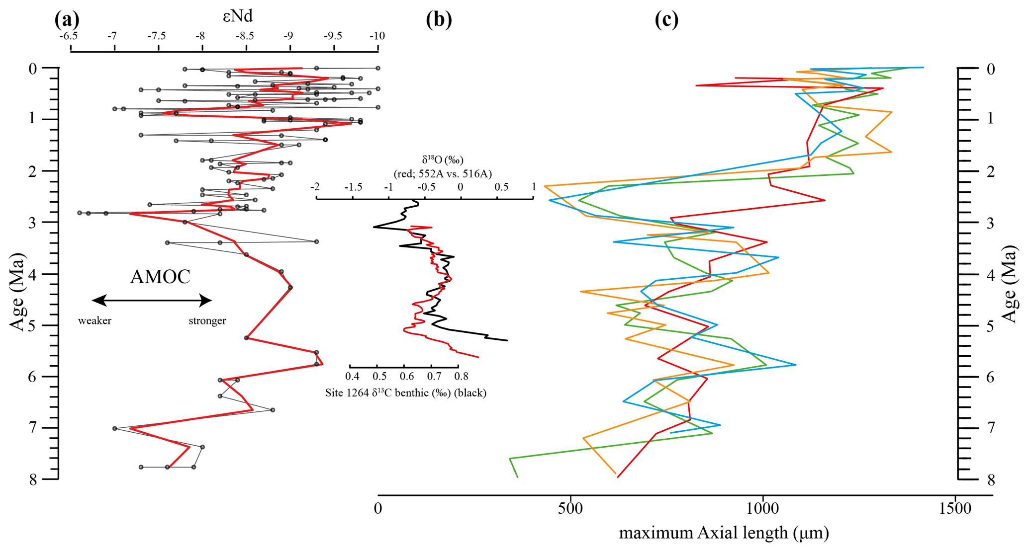
Figure 12Comparison of seawater Neodymium isotope evolution (εNd), a proxy for the strength of the AMOC, and the maximum axial length of Globorotalia menardii. (a) Dausmann et al. (2017): εNd at Site 1088 in the southern Atlantic Ocean. The thin black line shows the original data and the red line a smoothed version, produced with the RStudios' command “smooth.spline” at the value of 0.35. (b) AMOC strength reconstruction by Karas et al. (2017): the red line represents the δ18O seawater gradient of Sites 552A and 516A, while the black one is the benthic δ13C curve from Site 1264. (c) Maximum axial length (δY) versus age (Ma). The green line represents the size evolution of Hole 667A (eastern tropical Atlantic; this study), orange of Hole 925B (western tropical Atlantic; Knappertsbusch, 2015), blue of Site 502 (Caribbean Sea; Knappertsbusch, 2007b) and red of Site 503 (eastern tropical Pacific; Knappertsbusch, 2007c).
Although the maximum test size for Hole 667A also shows a similar trend to the AMOC strength reconstruction of Karas et al. (2017) for the Pliocene (Fig. 12b), the overall correlation between the maximum test size and the linear interpolation of εNd values by Dausmann et al. (2017) remains poor (R2 = 0.1477, Appendix Fig. A8). In the authors opinion, this result is not surprising. The system is most likely not strictly mechanistic, and there are a multitude of subtle interrelationships between ecology and the test size of G. menardii. In order to explain the missing strict, linear and cause-and-effect relationship, one may reason the following hypotheses:
-
The younger giant G. menardii form (0–2 Ma) may have occupied a (slightly) different ecology (ecological niche) in comparison to the ancestral Miocene–Pliocene form (2–8 Ma). The younger type thus might not have been affected in the same way by changes in the AMOC strength than the older form. Evidence for this explanation is given by Fig. A8a in the Appendix. It shows the correlation between linearly interpolated εNd values and the maximum size from Hole 667A for the time interval from 0 to 2 Ma (black points) and 2 to 8 Ma (red points), which fall into two groups. A similar observation is made in the WTAO Hole 925B, where the data allow a clear grouping into the new giant form (0–2 Ma, black dots) and the ancestral form (2–8 Ma, red dots; Fig. A8b in the Appendix).
-
Due to the closure of the Central American Seaway, the Atlantic's hydrography and oceanography altered, and the AMOC strength changed significantly (Haug and Tiedemann, 1998; Haug et al., 2001; Bartoli et al., 2005). The alterations maybe affected the way the AMOC strength influenced the environmental conditions within the Atlantic Ocean so that the AMOC had no major influence on the test size of G. menardii anymore.
The rough parallel trend between G. menardii test size and εNd between 2 and 8 Ma suggests a direct or indirect influence of the AMOC strength on the vertical thermal structure (Haarsma et al., 2008; dos Santos et al., 2010) of the upper-ocean water column in the tropical Atlantic Ocean.
Thus, changes in the strength of the AMOC may be invoked, which shifted the position of the ITCZ and associated trade winds (Billups et al., 1999; Timmermann et al., 2007), and which in turn affect the thermocline strength (Merle, 1983; Chaisson and Ravelo, 1997; Wolff et al., 1999). It is, for example, known that the ETAO thermocline reacts sensitively to variations in the AMOC strength (Haarsma et al., 2008; dos Santos et al., 2010). In this manner, the habitat of G. menardii would have been altered as well. A model for the response of test size of G. menardii under a changing thermocline is presented in the next section.
4.3 A thermocline model for size variation in G. menardii
A number of stable isotopic studies (Curry et al., 1983; Keller, 1985; Savin et al., 1985; Schweitzer and Lohmann, 1991; Gasperi and Kennett, 1992; Ravelo and Fairbanks, 1992; Gasperi and Kennett, 1993; Stewart, 2003; Steph et al., 2006; Mohtadi et al., 2009; Regenberg et al., 2010; Wejnert et al., 2010; Davis et al., 2019), plankton tows (Fairbanks et al., 1982; Thunell and Reynolds, 1984; Ravelo et al., 1990), census data from sediments (Sexton and Norris, 2011) and in situ observation (Hilbrecht and Thierstein, 1996) showed that G. menardii preferably dwells in the thermocline. According to Sexton and Norris (2011) and references therein, this coincides often with vertical habitats of increasing organic particle concentration and segregation, a zone in the thermocline where oxygen consumption due to particle degradation is high and where oxygen content becomes lowered.
Changes in the test size of PF are thought to be related to changes in the environmental conditions (Hecht, 1976; Malmgren and Kennett, 1976; Naidu and Malmgren, 1995; Schmidt et al., 2004; André et al., 2018), assuming that under optimum conditions, test size of species increases to its maximum, while under non-optimum conditions, the size is reduced, although detailed physiological processes at individual levels are still not entirely understood. However, Rillo et al. (2018) argued against the general validity of this hypothesis.
Assuming the “optimum-condition” hypothesis, Fig. 13 presents a model of how the thermocline strength could have influenced the test size of G. menardii: a strong thermocline leads to a stronger density gradient between the surface and the subsurface layer. Often the chlorophyll maximum zone is located at this boundary (Fairbanks et al., 1982; Ravelo and Fairbanks, 1992; Steph et al., 2006), where marine snow accumulates (Möller et al., 2012; Prairie et al., 2015). The increased concentration of degrading particulate organic matter enhances nutritional conditions and favours the test growth of G. menardii. It is, for example, known that nutrient-rich conditions facilitate test-size increase in the PF species Globigerinoides sacculifer (Bé et al., 1981), Globigerinoides ruber, Globigerinita glutinata, Globigerina bulloides and Neogloboquadrina dutertrei (Naidu and Malmgren, 1995). The thermocline may play a crucial role in other aspects of G. menardii's life cycle as well. A strong thermocline and the corresponding high-density contrast are thought to concentrate its gametes and food particles at a narrower zone and thus increase their chance to survive (Norris, 1999; Broecker and Pena, 2014).
This model of ecological factors within the regional thermocline influencing the phenotypic expression of G. menardii fits with Sexton and Norris' (2011) deglaciation proliferation model modulating the stratigraphic distribution of G. menardii. They suggest that G. menardii tracks thermoclines in areas with a moderately low oxygen concentration of ∼ 50–100 µmol kg−1, probably reduced by the degradation of organic matter.
Furthermore, Sexton and Norris (2011) postulate the reduction or vanishing of G. menardii populations during glacial times due to better-ventilated surface water masses, i.e. a weaker thermocline. Weakening of the AMOC during glacial times (Broecker, 1991; Berger and Wefer, 1996; Buizert and Schmittner, 2015) and associated changes in the position of the ITCZ led to a weakening and/or re-positioning of the thermocline so that ambient conditions became less suitable for growth and proliferation of G. menardii.
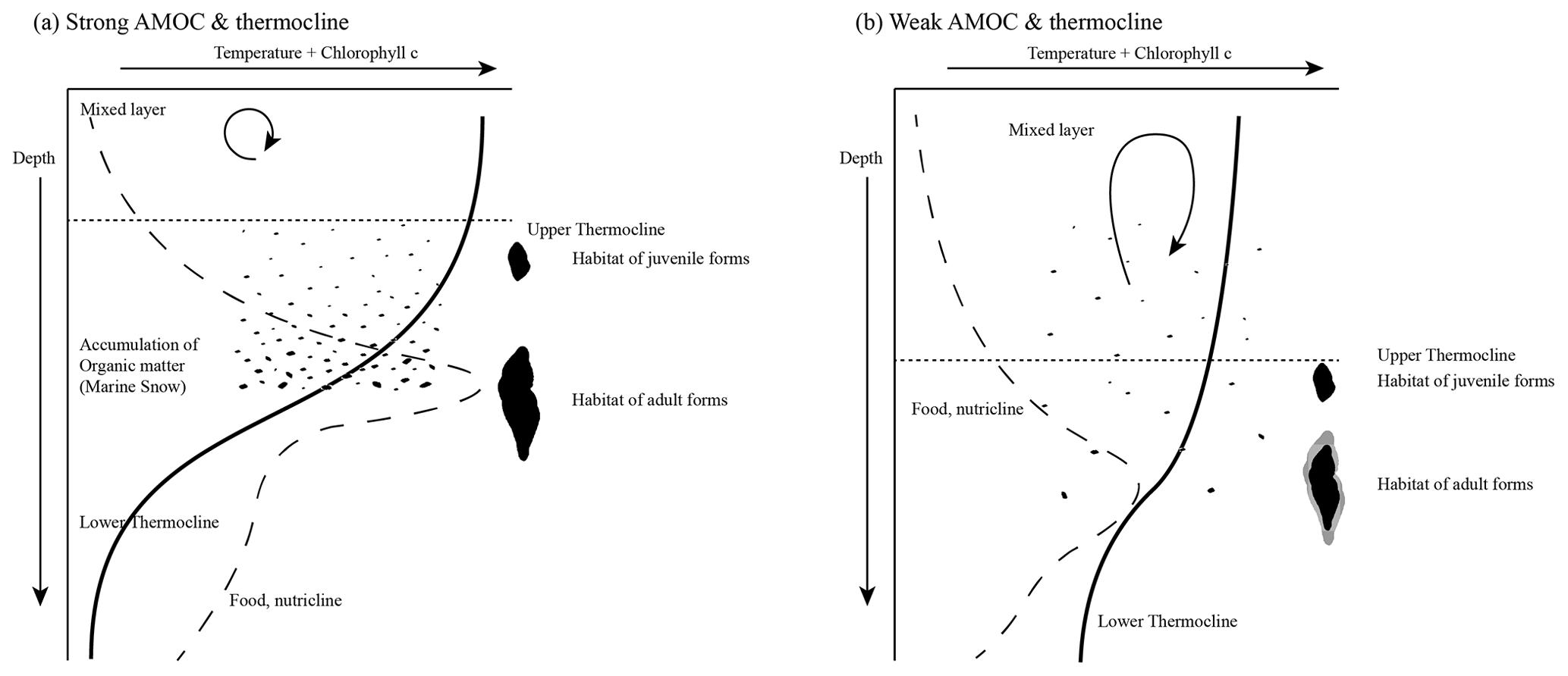
Figure 13Schematic illustration of the AMOC and thermocline hypothesis. Environmental conditions are expressed as changes in the relative temperature (solid line) and the chlorophyll concentration (dashed line) with increasing depth. (a) Relatively strong AMOC and thermocline. A thin mixed layer consists of relatively warm water, while the subsurface layer is cooler. It causes a strong temperature gradient and thus a strong thermocline. This results in an increased accumulation of organic matter (marine snow) and a high concentration of chlorophyll within the thermocline. The concentration of food and the physical conditions may favour the test growth of G. menardii. (b) A relatively cool and deep mixed layer and a warm subsurface layer develop a weak thermocline. In comparison to strong thermocline conditions, the accumulation of chlorophyll and organic matter is low. The physical conditions may also contribute to a reduction in the test growth of G. menardii. Illustration modified by Brown (2007).
The proposed thermocline hypothesis (Fig. 13) offers a possible way to explain the test-size evolution of the G. menardii lineage between 7.96 and 2.057 Ma within the tropical Atlantic Ocean, the Caribbean Sea and the Pacific Ocean, assuming analogous conditions.
A causal chain of physiological processes in order to explain the empirical similarity between the AMOC strength and the evolution of test size of G. menardii, however, still remains elusive and needs further investigation.
Test-size measurements of the planktonic foraminifer Globorotalia menardii from the eastern tropical Atlantic Ocean ODP Hole 667A show a striking size increase in the early Pleistocene and a test-size evolution during the past 8 Myr similar to observations done in the tropical Atlantic and Caribbean Sea (Knappertsbusch, 2007a, 2016). The giant forms of G. menardii occurred at ca. 2.06 Ma at Hole 667A, approximately 100 Kyr earlier than its occurrence in the western tropical Atlantic.
The coincidence of the relatively sudden size increase and the prominent change to sinistral coiling during the last 2 Myr give reason to suspect a new, giant G. menardii population in the Atlantic Ocean that is different from ancestral smaller forms. If true, this new menardiform would have appeared already in the eastern tropical Pacific since at least 2.58 Ma. It cannot be excluded that they have been dispersed from there throughout the Pacific and Indian Ocean, and then via Agulhas leakage into the Atlantic Ocean.
The test-size evolution within the time interval from ca. 8 to 2 Ma in the tropical Atlantic Ocean and Caribbean Sea shows a rough parallel trend with the isotopic εNd proxy for AMOC strength. It suggests that the stronger the AMOC becomes, the larger G. menardii grow. This empirical and so far preliminary observation suggests a causal relationship between menardiform test size, thermal upper-water stratification in the habitat of G. menardii and AMOC strength. Further studies are needed to confirm this hypothesis.
A combination of the Agulhas leakage hypothesis and the AMOC and thermocline hypothesis probably provides the most reasonable explanation for the observed Atlantic test-size evolution since the late Miocene, assuming that both models are related to each other. While the size evolution seemed to be influenced by the strength of the AMOC from 8 to ca. 2 Ma, the Agulhas leakage could have dispersed a new giant, sinistrally coiling G. menardii form from the Pacific Ocean via the Indian Ocean into the Atlantic Ocean within the time interval from 2.58 and 2.057 Ma. The establishment of a new giant form is probably related to a rapid improvement of the environmental conditions for G. menardii, such as a strengthening of the thermocline after the onset of the Northern Hemisphere Glaciation in the tropical Atlantic Ocean.
At present, the alternative hypothesis of a regional and punctuated evolutionary event cannot be dismissed until more palaeobiogeographic data are available at higher geographic resolution, especially from the Indian Ocean realm.
The results of this paper show that for an improvement of a taxonomic distinction between closely related species with high morphological overlap, it is strongly necessary to better include temporal measurements of morphological divergence.
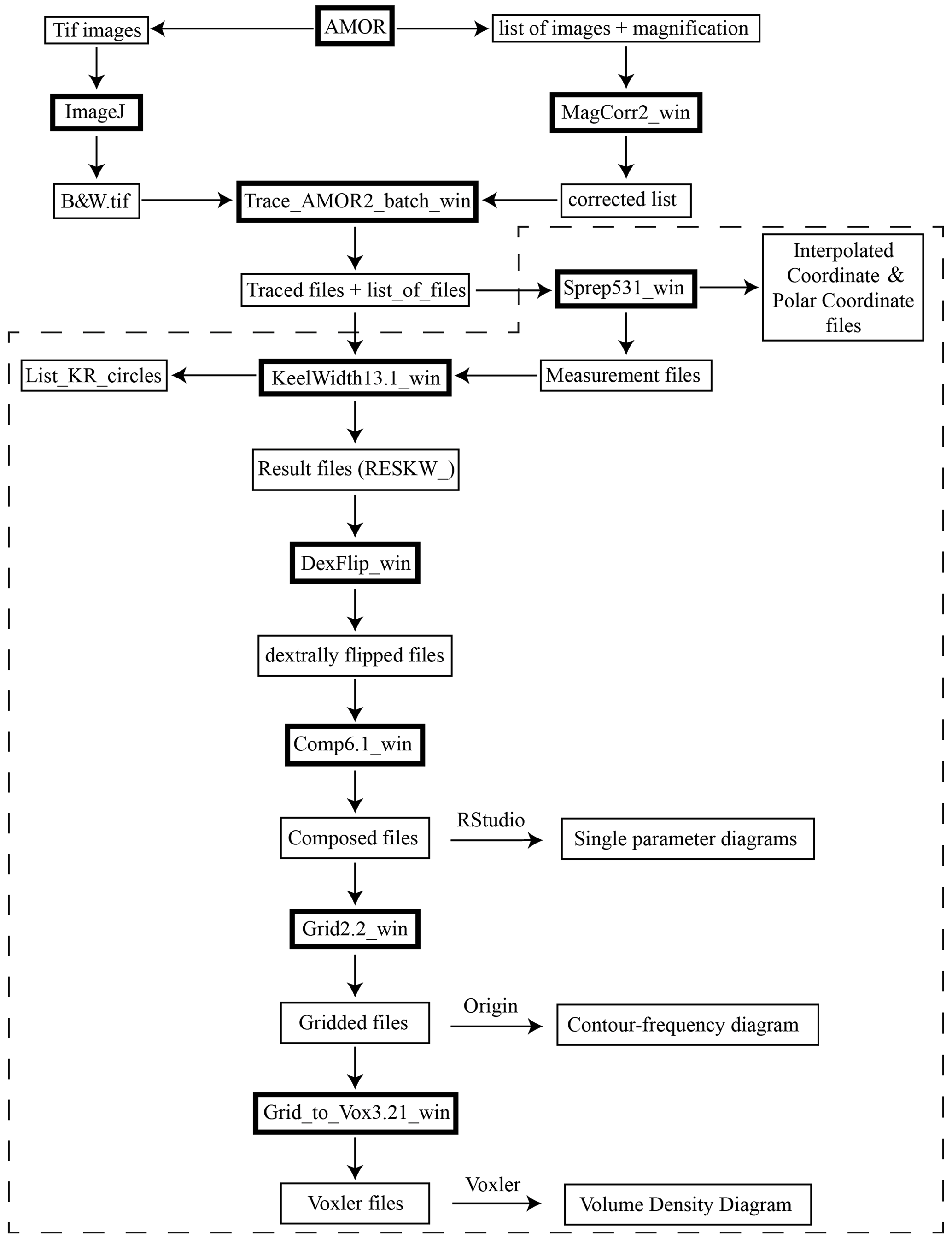
Figure A1Flow chart of MorphCol programmes used. The dashed frame indicates processing steps after sorting of files with respect to species, number of chambers in the final whorl and coiling direction.
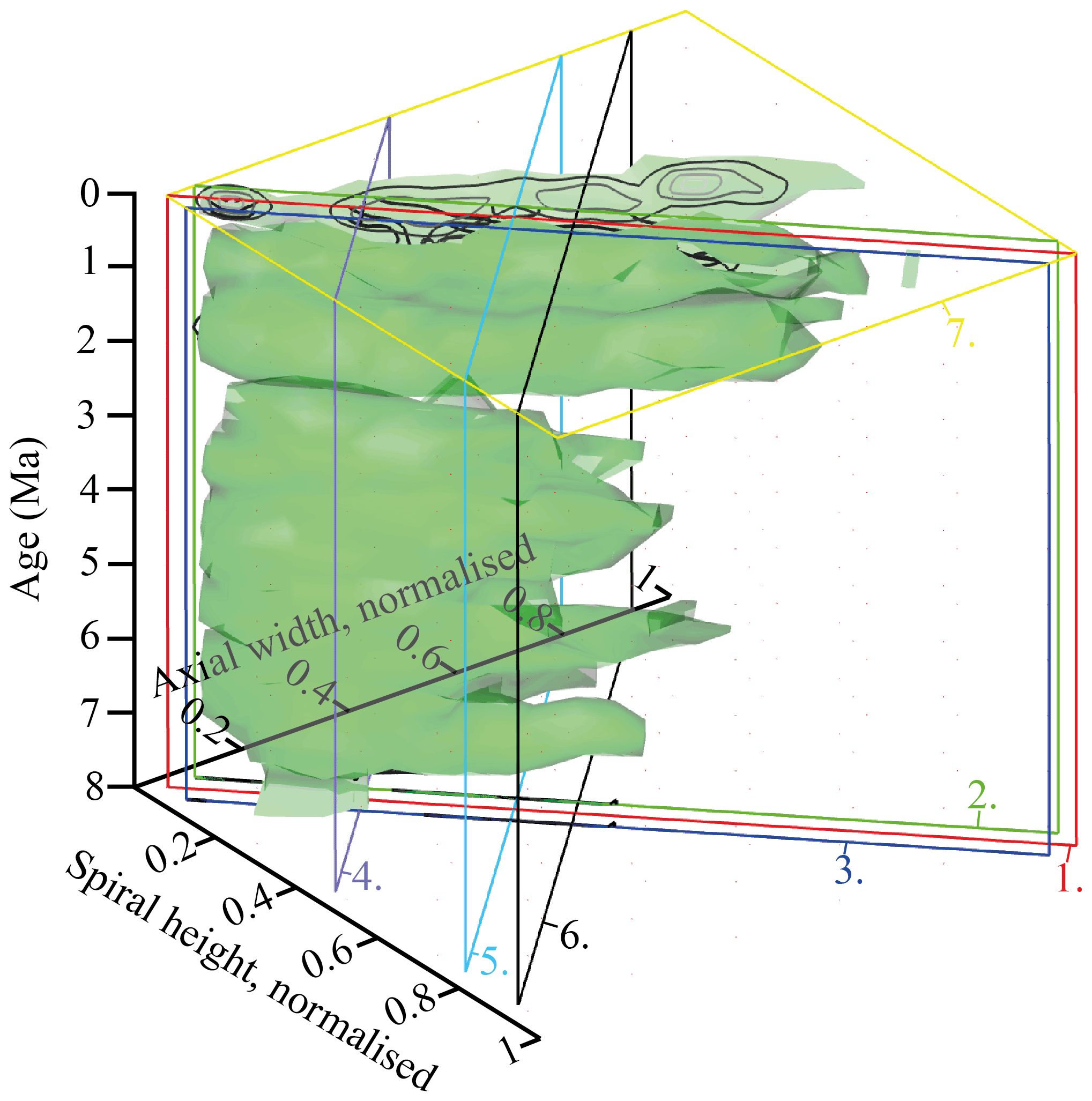
Figure A2VDD of normalised spiral height (δX) versus normalised axial length (δY) during the past 8 Myr for G. menardii. The position of the vertical frontal and sagittal sections shown in Figs. 10 and A3–A7 are indicated as coloured planes. The iso-surface (value = 0.89447168) represents the density of one specimen per grid cell. The red frontal section 1 is that of Fig. 10. Frontal section 2 (green) has an offset value of −0.05 (away from the reader; see Fig. A3). Frontal section 3 (blue) has an offset value of +0.05 (towards the reader; see Fig. A4). Sagittal section 4 (violet, offset = −0.55; Fig. A5), sagittal section 5 (light blue, offset value = −0.23; Fig. A6) and sagittal section 6 (black, offset = −0.1; Fig. A7) are orthogonally positioned in comparison to sections 1, 2 and 3. The yellow transversal plain at 0.003 Ma (7) shows the aberrant orientation of the contour frequency diagram in sample 667A-1H-1, 3–4 cm (see text). The black lines represent contour intervals of 3.
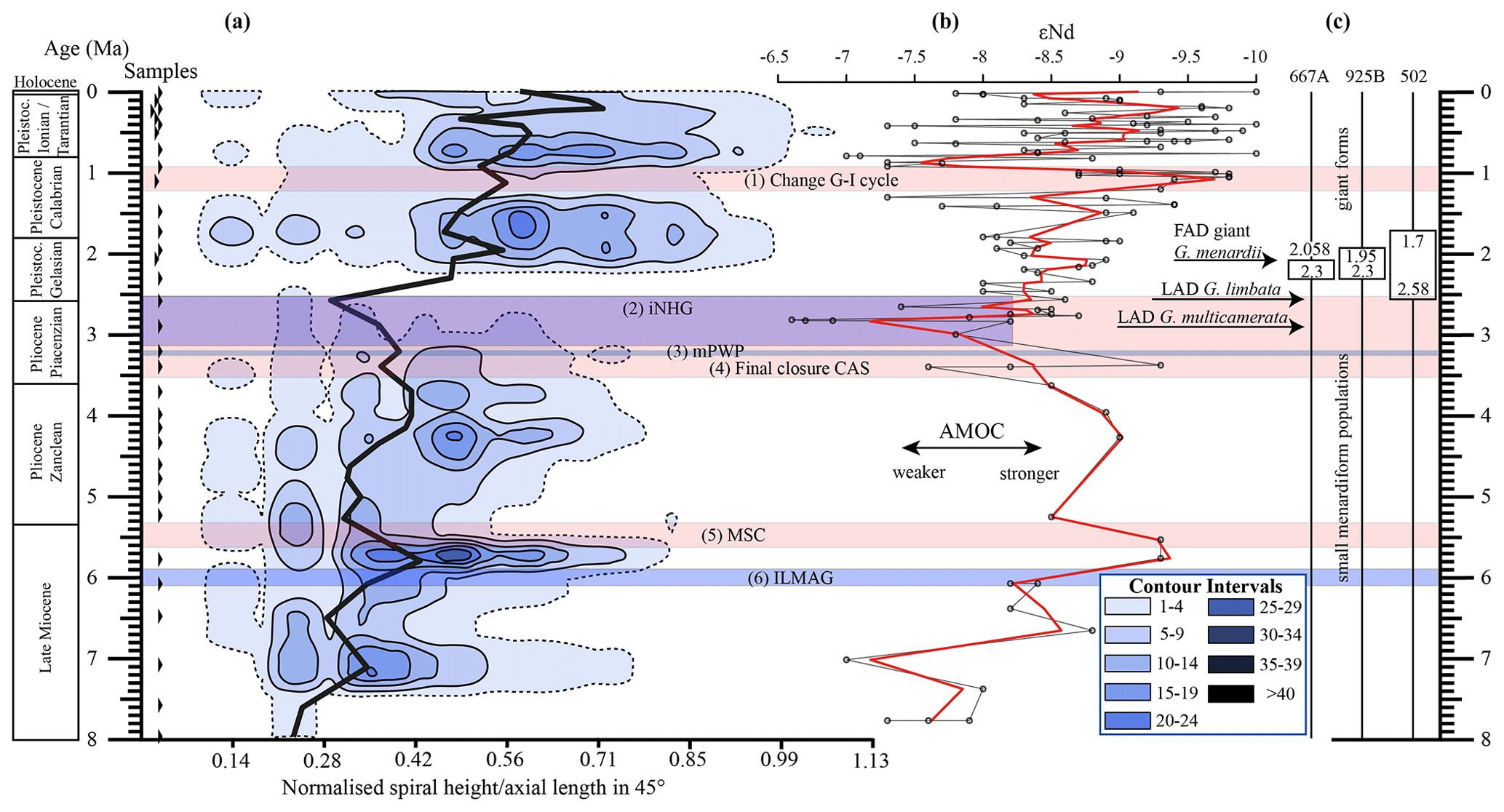
Figure A3Frontal section (offset value = −0.05, away from the reader) through the 45∘ view on VDD of Hole 667A in a palaeoceanographic context. The dotted line represents the interval line 1, and the solid lines show the contours with an interval of 5. The position of this section within the VDD is plotted in Fig. A2. For further explanation, see Fig. 10 in the text.
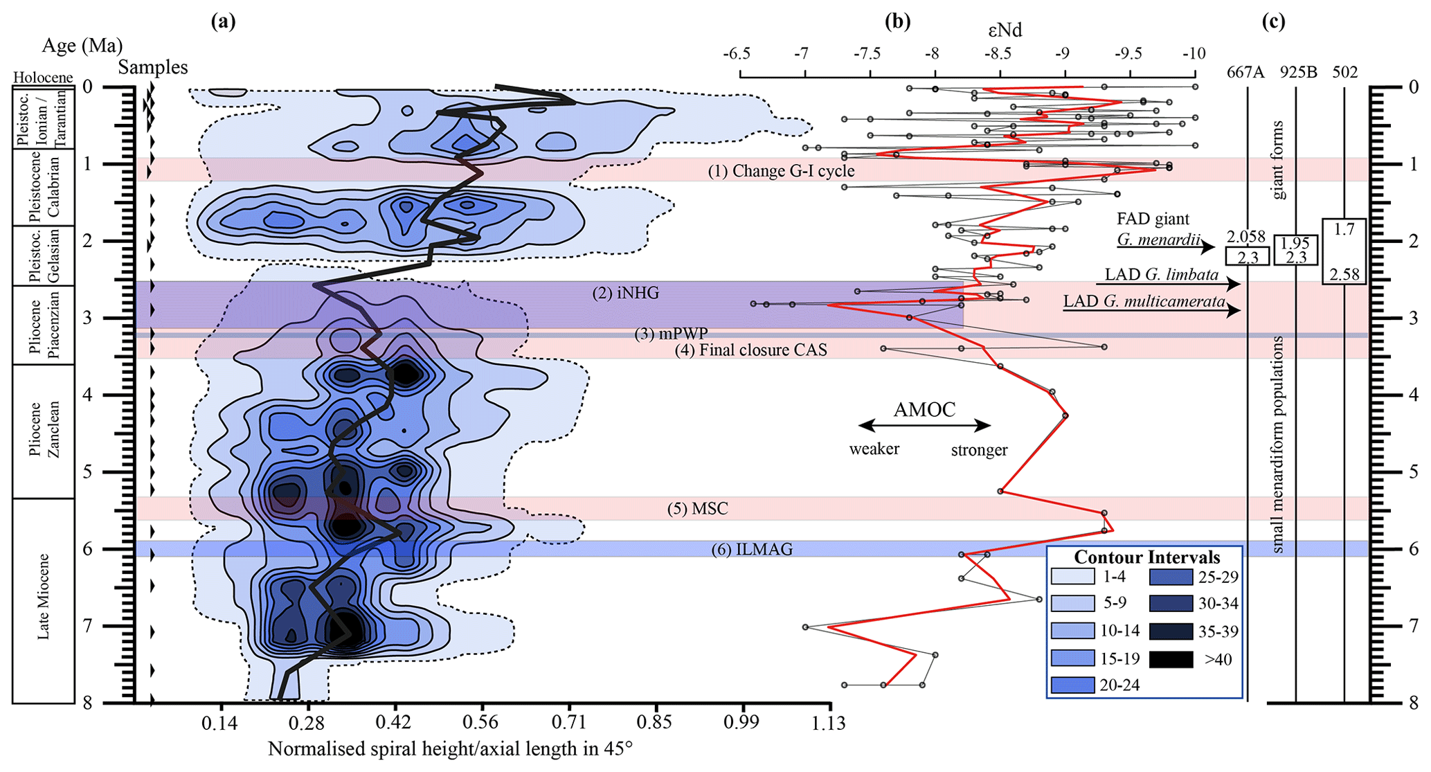
Figure A4Frontal section (offset value = +0.05, towards the reader) through the 45∘ view on VDD of Hole 667A in a palaeoceanographic context. The dotted line represents the interval line 1, and the solid lines show the contours with an interval of 5. The position of this section within the VDD is plotted in Fig. A2. For further explanation, see Fig. 10 in the text.
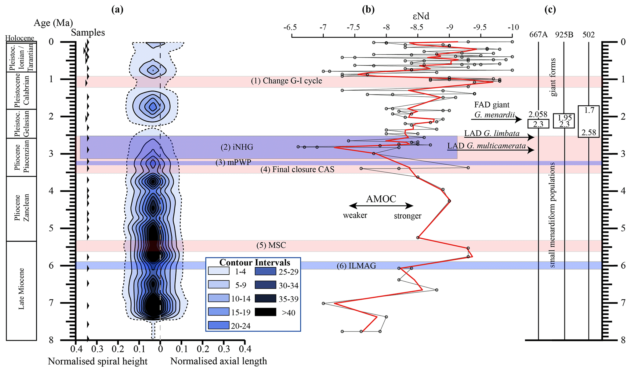
Figure A5Sagittal section with an offset value of −0.55 through the 135∘ view on the VDD of Hole 667A in a palaeoceanographic context. The dotted line represents the interval line 1, and the solid lines show the contours with an interval of 5. The vertical dashed line at x = 0 symbolises the position of the z axis, which is hidden behind the contour plot. The position of this section within the VDD is plotted in Fig. A2. For further explanation, see Fig. 10 in the text.
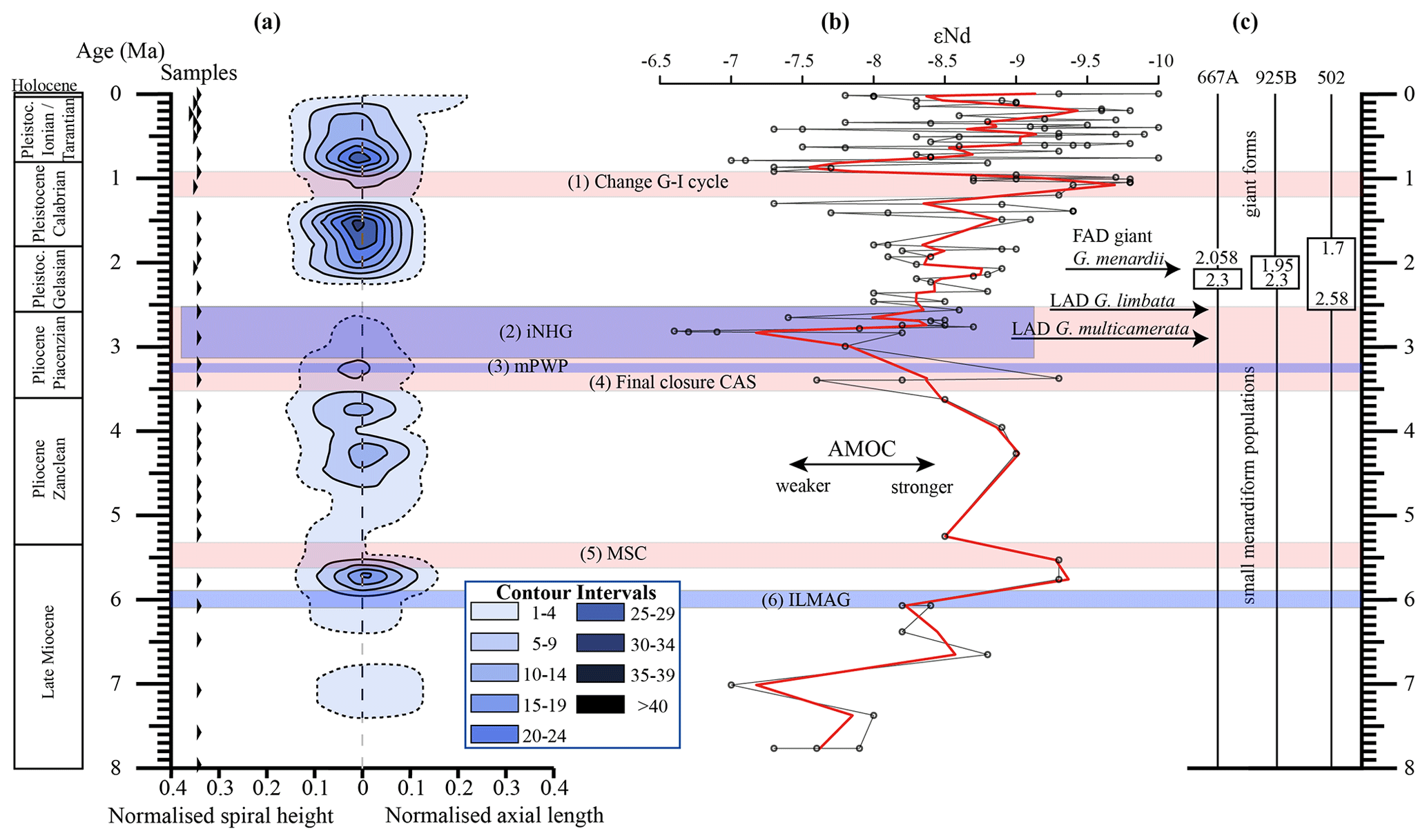
Figure A6Sagittal section with an offset value of −0.23 through the 135∘ view on the VDD of Hole 667A in a palaeoceanographic context. The dotted line represents the interval line 1, and the solid lines show the contours with an interval of 5. The vertical dashed line at x = 0 symbolises the position of the z axis, which is hidden behind the contour plot. The position of this section within the VDD is plotted in Fig. A2. For further explanation, see Fig. 10 in the text.
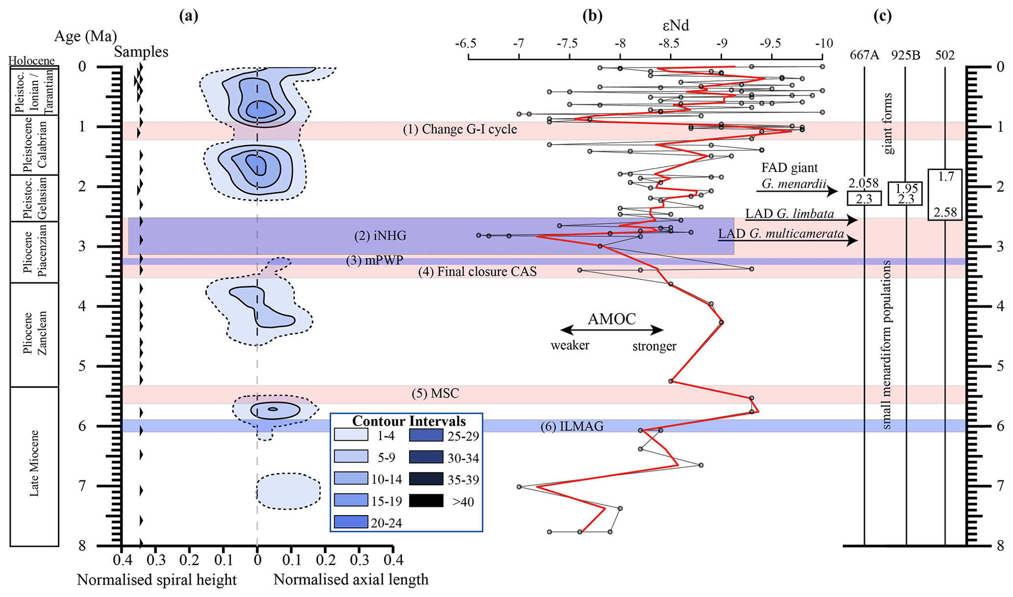
Figure A7Sagittal section with an offset value of −0.1 through the 135∘ view on the VDD of Hole 667A in a palaeoceanographic context. The dotted line represents the interval line 1, and the solid lines show the contours with an interval of 5. The vertical dashed line at x = 0 symbolises the position of the z axis, which is hidden behind the contour plot. The position of this section within the VDD is plotted in Fig. A3. For further explanation, see Fig. 10 in the text.

Figure A8Linearly interpolated εNd values derived from Dausmann et al. (2017) plotted versus the maximum axial length (δY) of G. menardii from 33 sediment samples from Hole 667A and 29 samples from Hole 925B. The samples have an age of up to 8 Ma (Table 1, this study; Knappertsbusch 2016, respectively). (a) Correlation between εNd and δY for all samples of Hole 667A. Black points represent samples with an age between 0 and 2 Ma and red dots samples with an age between 2 and 8 Ma. The black line (1) is the coefficient of determination (R2) for samples with an age of 0–2 Ma and the red one (2) for samples from 2 to 8 Ma. (b) Correlation between εNd and δY for samples of Hole 925B. Red dots represent samples from time intervals 8 to 2 Ma. The bottom-left corner shows the corresponding R2 and p values.
The modified MorphCol programmes, which were used to process the raw data, as well as their codes, will be available at PANGAEA (Friesenhagen, 2022).
The full set of derived and raw data and images will be deposited at PANGAEA (Friesenhagen, 2022). The supplied zip archive Supplement is an extract of all data and contains the necessary data to reproduce the illustrated figures.
The sample material is deposited in the collections of the Natural History Museum Basel, Switzerland, as the reference collection to Friesenhagen (2022).
The supplement related to this article is available online at: https://doi.org/10.5194/bg-19-777-2022-supplement.
The contact author has declared that there are no competing interests.
Publisher's note: Copernicus Publications remains neutral with regard to jurisdictional claims in published maps and institutional affiliations.
Thanks go to the Swiss National Science Foundation (SNF) for funding of this project (SNF nos. 200021_169048/1 and 200021_169048/2). The International Ocean Discovery Program is greatly acknowledged for providing the sample material used in this study (IODP request #047348IODP from 6 December 2016). Without the excellent collaboration with the staff of the Natural History Museum Basel and especially Michael Knappertsbusch, curator of the Geoscience department and initiator and supervisor of this project, this study would not have been possible. Special thanks go to the three anonymous reviewers and the commentator, Nisan Sariaslan, for giving valuable feedback and their help to improve this paper. I would like to thank Stefanie Schumacher of the PANGAEA editorial team for her effort. Last but not least, I am especially obliged to Loïc Costeur, Christian De Capitani, Thomas Kuhn, Bastien Mennecart, Johannes Pietsch, Diana Isabel Rendon Mera, Anja Studer and Alexandra Viertler for feedback, discussions, corrections and support.
This research has been supported by the Swiss National Science Foundation (SNF) (grant nos. 200021_169048/1 and 200021_169048/2).
This paper was edited by Markus Kienast and reviewed by three anonymous referees.
André, A., Weiner, A., Quillévéré, F., Aurahs, R., Morard, R., Douady, C. J., de Garidel-Thoron, T., Escarguel, G., de Vargas, C., and Kucera, M.: The cryptic and the apparent reversed: lack of genetic differentiation within the morphologically diverse plexus of the planktonic foraminifer Globigerinoides sacculifer, Paleobiology, 39, 21–39, https://doi.org/10.5061/dryad.rb06j, 2013.
André, A., Quillévéré, F., Schiebel, R., Morard, R., Howa, H., Meilland, J., and Douady, C. J.: Disconnection between genetic and morphological diversity in the planktonic foraminifer Neogloboquadrina pachyderma from the Indian sector of the Southern Ocean, Mar. Micropaleontol., 144, 14–24, https://doi.org/10.1016/j.marmicro.2018.10.001, 2018.
Bard, E. and Rickaby, R. E. M.: Migration of the subtropical front as a modulator of glacial climate, Nature, 460, 380–383, https://doi.org/10.1038/nature08189, 2009.
Bartoli, G., Sarnthein, M., Weinelt, M., Erlenkeuser, H., Garbe-Schönberg, D., and Lea, D. W.: Final closure of Panama and the onset of northern hemisphere glaciation, Earth Planet. Sc. Lett., 237, 33–44, https://doi.org/10.1016/j.epsl.2005.06.020, 2005.
Bé, A. W. H., Caron, D. A., and Anderson, O. R.: Effects of feeding frequency on life processes of the planktonic foraminifer Globigerinoides sacculifer in laboratory culture, J. Mar. Biol. Assoc. UK, 61, 257–277, https://doi.org/10.1017/s002531540004604x, 1981.
Beal, L. M., De Ruijter, W. P. M., Biastoch, A., and Zahn, R.: On the role of the Agulhas system in ocean circulation and climate, Nature, 472, 429–436, https://doi.org/10.1038/nature09983, 2011.
Berger, W. H. and Wefer, G.: Expeditions into the Past: Paleoceanographic Studies in the South Atlantic, in: The South Atlantic, Springer Berlin Heidelberg, 363–410, https://doi.org/10.1007/978-3-642-80353-6_21, 1996.
Berggren, W. A., Kent, D. V., Swisher, C. C., and Aubry, M.-P.: A Revised Cenozoic Geochronology and Chronostratigraphy, in: Geochronology, time scales and global stratigraphic correlation, edited by: Aubry, M. P. and Hardenbol, J., SEPM (Society for Sedimentary Geology), 54, 129–212, https://doi.org/10.2110/pec.95.04.0129, 1995.
Bermúdez, P. J. and Bolli, H. M.: Consideraciones sobre los sedimentos del Mioceno medio al Reciente de las costas central y oriental de Venezuela, Boletin de Geologia, Ministerio de Minas e Hidrocarburos, 10, 137–223, 1969.
Biastoch, A., Böning, C. W., Schwarzkopf, F. U., and Lutjeharms, J. R. E.: Increase in Agulhas leakage due to poleward shift of Southern Hemisphere westerlies, Nature, 462, 495–498, https://doi.org/10.1038/nature08519, 2009.
Billups, K., Ravelo, A. C., Zachos, J. C., and Norris, R. D.: Link between oceanic heat transport, thermohaline circulation, and the Intertropical Convergence Zone in the early Pliocene Atlantic, Geology, 27, 319–322, https://doi.org/10.1130/0091-7613(1999)027<0319:lbohtt>2.3.co;2, 1999.
Blaser, P., Frank, M., and van der Flierdt, T.: Revealing past ocean circulation with neodymium isotopes, Past Glob. Chang. Mag., 27, 54–55, https://doi.org/10.22498/pages.27.2.54, 2019.
Bolli, H. M.: The direction of coiling in the evolution of some Globorotaliidae, Contributions from the Cushman Foundation for Foraminiferal Research, 1, 82–89, 1950.
Bolli, H. M.: Initial Reports of the Deep Sea Drilling Project, Vol. IV, chap. 25, The Foraminifera of Sites 23-31, LEG 4, U.S. Government Printing Office, 577–644, https://doi.org/10.2973/dsdp.proc.4.125.1970, 1970.
Bolli, H. M. and Premoli Silva, I.: Oligocene to Recent Planktonic Foraminifera and Stratigraphy of the Leg 15 Sites in the Caribbean Sea, in: Initial Reports of the Deep Sea Drilling Project, 15, edited by: Edgar, N. T., Kaneps, A. G., and Herring, J. R., U.S. Government Printing Office, Vol. 15, 475–497, https://doi.org/10.2973/dsdp.proc.15.110.1973, 1973.
Bolli, H. M. and Saunders, J. B.: Plankton Stratigraphy, chap. 6, Oligocene to Holocene low latitude planktic foraminifera, Cambridge University Press, 1, 155–262, ISBN 0521235766, 1985.
Broecker, W. S.: The Great Ocean Conveyor. Oceanography, 4, 79–89, https://doi.org/10.5670/oceanog.1991.07, 1991.
Broecker, W. S. and Pena, L. D.: Delayed Holocene reappearance of G. menardii, Paleoceanogr. Paleocl., 29, 291–295, https://doi.org/10.1002/2013PA002590, 2014.
Brombacher, A., Wilson, P. A., Bailey, I., and Ezard, T. H. G.: The Breakdown of Static and Evolutionary Allometries during Climatic Upheaval, Am. Nat., 190, 350–362, https://doi.org/10.1086/692570, 2017.
Brombacher, A., Wilson, P. A., Bailey, I., and Ezard, T. H. G.: The Dynamics of Diachronous Extinction Associated With Climatic Deterioration Near the Neogene/Quaternary Boundary, Paleoceanogr. Paleocl., 36, e2020PA004205, https://doi.org/10.1029/2020PA004205, 2021.
Brown, K. R.: Biogeographic and morphological variation in late Pleistocene to Holocene globorotalid foraminifera, Ph.D. thesis, University of Basel, available at: https://edoc.unibas.ch/780/ (last access: 20 June 2012), 2007.
Buizert, C. and Schmittner, A.: Southern Ocean control of glacial AMOC stability and Dansgaard-Oeschger interstadial duration, Paleoceanography, 30, 1595–1612, https://doi.org/10.1002/2015pa002795, 2015.
Caley, T., Jiraudeau, J., Malaizé, B., Rossignol, L., and Pierre, C.: Agulhas leakage as a key process in the modes of Quaternary climate changes, P. Natl. Acad. Sci. USA, 109, 6835–6839, https://doi.org/10.1073/pnas.1115545109, 2012.
Caromel, A. G. M., Schmidt, D. N., Fletcher, I., and Rayfield, E. J.: Morphological Change During The Ontogeny Of The Planktic Foraminifera, J. Micropalaeontol, 35, 2–19, https://doi.org/10.1144/jmpaleo2014-017, 2016.
Chaisson, W. P.: Vicarious living: Pliocene menardellids between an isthmus and an ice sheet, Geology, 31, 1085–1088, https://doi.org/10.1130/G19834.1, 2003.
Chaisson, W. P. and Ravelo, A. C.: Changes in upper water-column structure at Site 925, late Miocene-Pleistocene: planktonic foraminifer assemblage and isotopic evidence, in: Proceedings of the Ocean Drilling Program, edited by: Shackleton, N. J., Curry, W. B., Richter, C., and Bralower, T. J., College Station, TX (Ocean Drilling Program), Vol. 154, 255–268, https://doi.org/10.2973/odp.proc.sr.154.105.1997, 1997.
Chan, C.-H., Chan, G. C. H., Leeper, T. J., and Becker, J.: rio: A Swiss-army knife for data file I/O, r package version 0.5.16, https://cran.r-project.org/src/contrib/Archive/rio/ (last access: 7 September 2021), 2018.
Chapman, M. R.: Biotic Response to Global Changes: The Last 145 Million Years, The response of planktonic foraminifera to the Late Pliocene intensification of Northern Hemisphere glaciation, 115, 79–96, Cambridge University Press, https://doi.org/10.1017/CBO9780511535505.007, 2000.
Clemens, S. C., Murray, D. W., and Prell, W. L.: Nonstationary Phase of the Plio-Pleistocene Asian Monsoon, Science, 274, 943–948, https://doi.org/10.1126/science.274.5289.943, 1996.
Clyde-Brockway, C. E.: Inter-Nesting and Post-Nesting Movements and Behavior of East Pacific Green Turtles (Cheloniamydas agassizii) from Playa Cabuyal, Guanacaste, Costa Rica, Masterthesis, Indiana University – Purdue University Fort Wayne, ProQuest Dissertations Publishing, 2014.
Curry, W. B., Thunell, R. C., and Honjo, S.: Seasonal changes in the isotopic composition of planktonic foraminifera collected in Panama Basin sediment traps, Earth Planet. Sc. Lett., 64, 33–43, https://doi.org/10.1016/0012-821x(83)90050-x, 1983.
Dausmann, V., Frank, M., Gutjahr, M., and Rickli, J.: Glacial reduction of AMOC strength and long–term transition in weathering inputs into the Southern Ocean since the mid–Miocene: Evidence from radiogenic Nd and Hf isotopes, Paleoceanography, 32, 265–283, https://doi.org/10.1002/2016PA003056, 2017.
Davis, C. V., Fuqua, L., Pride, C., and Thunell, R.: Seasonal and interannual changes in planktic foraminiferal fluxes and species composition in Guaymas Basin, Gulf of California, Mar. Micropaleontol., 149, 78–88, https://doi.org/10.1016/j.marmicro.2019.05.001,2019.
dos Santos, R. A. L., Prange, M., Castañeda, I. S., Schefuß, E., Mulitza, S., Schulz, M., Niedermeyer, E. M., Damsté, J. S. S., and Schouten, S.: Glacial-interglacial variability in Atlantic meridional overturning circulation and thermocline adjustments in the tropical North Atlantic, Earth Planet. Sc. Lett., 300, 407–414, https://doi.org/10.1016/j.epsl.2010.10.030, 2010.
Ericson, D. B. and Wollin, G.: Micropaleontological and isotopical determinations of Pleistocene climates, Micropaleontology, 2, 257–270, https://doi.org/10.2307/1484180, 1956.
Fairbanks, R. G., Sverdlove, M., Free, R., Wiebe, H. P., and Bé, A. W. H.: Vertical distribution and isotopic fractionation of living planktonic foraminifera from the Panama Basin, Nature, 298, 841–844, https://doi.org/10.1038/298841a0, 1982.
Friesenhagen, T.: Archive to the evolutionary study about menardiform globorotallids (planktonic foraminifer) in the eastern tropical Atlantic ocean ODP Hole 667A, PANGAEA [data set and code], https://doi.pangaea.de/10.1594/PANGAEA.940563, 2022.
Gasperi, J. T. and Kennett, J. P.: Pacific Neogene-Environment, Evolution, and Events, Biostratigraphy and paleoceanography of the Japan Sea based on diatoms: ODP Leg 127, chap. Isotopic Evidence for Depth Stratification and Paleoecology of Miocene Planktonic Foraminifera, Tokyo, University of Tokyo Press, 117–147, ISBN 0 86008 491 4, ISBN 4 13 068206 7, 1992.
Gasperi, J. T. and Kennett, J. P.: Vertical thermal structure evolution of Miocene surface waters Western equatorial Pacific DSDP Site 289, Mar. Micropaleontol., 22, 235–254, https://doi.org/10.1016/0377-8398(93)90046-Z, 1993.
Haarsma, R. J., Campos, E., Hazeleger, W., and Severijns, C.: Influence of the Meridional Overturning Circulation on Tropical Atlantic Climate and Variability, J. Clim., 21, 1403–1416, https://doi.org/10.1175/2007JCLI1930.1, 2008.
Haug, G. H. and Tiedemann, R.: Effect of the formation of the Isthmus of Panama on Atlantic Ocean thermohaline circulation, Nature, 393, 673–676, https://doi.org/10.1038/31447, 1998.
Haug, G. H., Tiedemann, R., Zahn, R., and Ravelo, A. C.: Role of Panama uplift on oceanic freshwater balance, Geology, 29, 207–210, https://doi.org/10.1130/0091-7613(2001)029<0207:ROPUOO>2.0.CO;2, 2001.
Haywood, A. M., Dowsett, H. J., and Dolan, A. M.: Integrating geological archives and climate models for the mid-Pliocene warm period, Nat. Commun., 7, 10646, https://doi.org/10.1038/ncomms10646, 2016.
Hecht, A. D.: An ecologic model for test size variation in Recent planktonic foraminifera; applications to the fossil record, J. Foramin. Res., 6, 295–311, https://doi.org/10.2113/gsjfr.6.4.295,1976.
Hilbrecht, H. and Thierstein, H. R.: Benthic behavior of planktic foraminifera, Geology, 24, 200–202, https://doi.org/10.1130/0091-7613(1996)024<0200:BBOPF>2.3.CO;2, 1996.
Hull, P. M. and Norris, R. D.: Evidence for abrupt speciation in a classic case of gradual evolution, P. Natl. Acad. Sci. USA, 106, 21224–21229, https://doi.org/10.1073/pnas.0902887106, 2009.
Ivanova, E. V.: Paleoceanography of the Northern Indian Ocean: Linkages to Monsoon and Global Thermohaline Paleocirculation, in: The Global Thermohaline Paleocirculation, Springer Netherlands, 107–145, https://doi.org/10.1007/978-90-481-2415-2_5, 2009.
Karas, C., Nürnberg, D., Bahr, A., Groeneveld, J., Herrle, J. O., Tiedemann, R., and deMenocal, P. B.: Pliocene oceanic seaways and global climate, Sci. Rep., 7, 39842, https://doi.org/10.1038/srep39842, 2017.
Jackson, J. B. C. and O'Dea, A.: Timing of the oceanographic and biological isolation of the Caribbean Sea from the tropical eastern Pacific Ocean, Bull. Mar. Sci., 89, 779–800, https://doi.org/10.5343/bms.2012.1096, 2013.
Kämpf, J. and Chapman, P.: The Peruvian-Chilean Coastal Upwelling System, in: Upwelling Systems of the World, Springer International Publishing, 161–202, https://doi.org/10.1007/978-3-319-42524-5_5, 2016. 2016.
Keller, G.: Depth stratification of planktonic foraminifers in the Miocene ocean, in: Geological Society of America Memoirs, Geol. Soc. Am., 163, 177–196, https://doi.org/10.1130/mem163-p177, 1985.
Kennett, J. P. and Srinivasan, M. S.: Neogene planktonic foraminifera. A phylogenetic atlas, Hutchinson Ross Publishing Company, Stroudsburg, Pa, New York, NY, ISBN 0879330708, 1983.
Knappertsbusch, M. W.: Morphological variability of Globorotalia menardii (planktonic foraminifera) in two DSDP cores from the Caribbean Sea and the Eastern Equatorial Pacific, Carnets de Geologie, CG2007, hal-00164930, 2007a.
Knappertsbusch, M. W.: Morphometric data and processing steps of planktonic foraminifera from DSDP Site 68-502, PANGAEA, https://doi.org/10.1594/PANGAEA.863573, 2007b.
Knappertsbusch, M. W.: Morphometric data and processing steps of planktonic foraminifera from DSDP Site 68-503, PANGAEA, https://doi.org/10.1594/PANGAEA.863575, 2007c.
Knappertsbusch, M. W.: Evolution im marinen Plankton, Mitteilungen der Naturforschenden Gesellschaften beider Basel, 13, 3–14, https://doi.org/10.5169/seals-676589, 2011.
Knappertsbusch, M. W.: Raw-data to morphometric investigations about the Neogene planktonic foraminifer Globorotalia menardii and related forms from ODP Hole 154-925B (Céara Rise, western tropical Atlantic), PANGAEA, https://doi.org/10.1594/PANGAEA.855900, 2015.
Knappertsbusch, M. W.: Evolutionary prospection in the Neogene planktic foraminifer Globorotalia menardii and related forms from ODP Hole 925B (Ceara Rise, western tropical Atlantic): evidence for gradual evolution superimposed by long distance dispersal?, Swiss J. Palaeontol., 135, 205–248, https://doi.org/10.1007/s13358-016-0113-6, 2016.
Knappertsbusch, M. W. and Mary, Y.: Mining morphological evolution in microfossils using volume density diagrams, Palaeontologica Electronica, 15, 1–29, https://doi.org/10.26879/278, 2012.
Knappertsbusch, M. W., Binggeli, D., Herzig, A., Schmutz, L., Stapfer, S., Schneider, C., Eisenecker, J., and Widmer, L.: Amor – A New System For Automated Imaging Of Microfossils For Morphometric Analyses, Palaeontologia Electronica, 121, 12.2.2T, 2009.
Krijgsman, W., Hilgen, F. J., Raffi, I., Sierro, F. J., and Wilson, D. S.: Chronology, causes and progression of the Messinian salinity crisis, Nature, 400, 652–655, https://doi.org/10.1038/23231, 1999.
Lamb, J. L. and Beard, J. H.: Late Neogene planktonic foraminifers in the Caribbean, Gulf of Mexico and Italian stratotypes, Harold Norman Fisk Memorial Papers, The University of Kansas Paleontological Contributions, 57, 128921806, 1972.
Laxenaire, R., Speich, S., Blanke, B., Chaigneau, A., Pegliasco, C., and Stegner, A.: Anticyclonic Eddies Connecting the Western Boundaries of Indian and Atlantic Oceans, J. Geophys. Res.-Ocean., 123, 7651–7677, https://doi.org/10.1029/2018JC014270, 2018.
Lazarus, D.: Tempo and mode of morphologic evolution near the origin of the radiolarian lineage Pterocanium prismatium, Paleobiology, 12, 175–189, https://doi.org/10.1017/s0094837300013646, 1986.
Lazarus, D.: Age Depth Plot and Age Maker: Age Modeling of Stratigraphic Sections on the Macintosh Series of Computers, Geobyte, 7, 7–14, 5425155, 1992.
Lutjeharms, J. R. E. and Van Ballegooyen, R. C.: The Retroflection of the Agulhas Current, J. Phys. Oceanogr., 18, 1570–1583, https://doi.org/10.1175/1520-0485(1988)018<1570:TROTAC>2.0.CO;2, 1988.
Malmgren, B. A. and Kennett, J. P.: Biometric analysis of phenotypic variation in Recent Globigerina bulloides d'Orbigny in the southern Indian Ocean, Mar. Micropaleontol., 1, 3–25, https://doi.org/10.1016/0377-8398(76)90003-7, 1976.
Malmgren, B. A., Berggren, W. A., and Lohmann, G. P.: Evidence for punctuated gradualism in the Late Neogene Globorotalia tumida lineage of planktonic foraminifera, Paleobiology, 9, 377–389, https://doi.org/10.1017/s0094837300007843, 1983.
Manivit, H.: Calcareous Nannofossil Biostratigraphy in Leg 108 Sediments, in: Proc. ODP, Sci. Results 108, edited by: Baldauf, J., Heath, G. R., Ruddiman, W. F., and Sarnthein, M., College Station, TX (Ocean Drilling Program), Vol. 108, 35–69, https://doi.org/10.2973/odp.proc.sr.108.126.1989, 1989.
Mary, Y.: Morphologic, biogeographic and ontogenetic investigation of Mid-Pliocene menardellids (planktonic foraminifera), Ph.D. thesis, University of Basel, https://doi.org/10.5451/unibas-006194467, 2013.
McCarthy, G., Smeed, D., Cunningham, S., and Roberts, C.: Atlantic Meridional Overturning Circulation, MCCIP Science Review 2017, MCCIP, Lowestoft, UK, 15–21, https://doi.org/10.14465/2017.ARC10.002-ATL, 2017.
Merino, M. and Monreal-Gómez, M. A.: Marine Ecology, Ocean Currents and Their Impact on Marine Life, Eolss Publishers Co. Ltd., Oxford, 52–74, ISBN 978-1-84826-464-9, 2009.
Merle, J.: Seasonal Variability of Subsurface Thermal Structure in the Tropical Atlantic Ocean, in: Hydrodynamics of The Equatorial Ocean, Proceedings of The 14th International Liege Colloquium on Ocean Hydrodynamics, Elsevier, 31–49, https://doi.org/10.1016/s0422-9894(08)70626-3, 1983.
Mohtadi, M., Steinke, S., Groeneveld, J., Fink, H. G., Rixen, T., Hebbeln, D., Donner, B., and Herunadi, B.: Low-latitude control on seasonal and interannual changes in planktonic foraminiferal flux and shell geochemistry off south Java: A sediment trap study, Paleoceanography, 24, PA1201, https://doi.org/10.1029/2008pa001636, 2009.
Möller, K. O., John, M. S., Temming, A., Floeter, J., Sell, A. F., Herrmann, J.-P., and Möllmann, C.: Marine snow, zooplankton and thin layers: indications of a trophic link from small-scale sampling with the Video Plankton Recorder, Mar. Ecol. Prog. Ser., 468, 57–69, https://doi.org/10.3354/meps09984, 2012.
Naidu, P. D. and Malmgren, B. A.: Monsoon upwelling effects on test size of some planktonic foraminiferal species from the Oman Margin, Arabian Sea, Paleoceanography, 10, 117–122, https://doi.org/10.1029/94pa02682, 1995.
Niemitz, M. D. and Billups, K.: Millennial-scale variability in western tropical Atlantic surface ocean hydrography during the early Pliocene, Mar. Micropaleontol., 54, 155–166, https://doi.org/10.1016/j.marmicro.2004.10.001, 2005.
Norris, R. D.: Reconstruction Ocean History, Hydrographic and tectonic control of plankton distribution and evolution, Springer US, 173–193, https://doi.org/10.1007/978-1-4615-4197-4, 1999.
O'Dea, A., Lessios, H. A., Coates, A. G., Eytan, R. I., Restrepo-Moreno, S. A., Cione, A. L., Collins, L. S., de Queiroz, A., Farris, D. W., Norris, R. D., Stallard, R. F., Woodburne, M. O., Aguilera, O., Aubry, M.-P., Berggren, W. A., Budd, A. F., Cozzuol, M. A., Coppard, S. E., Duque-Caro, H., Finnegan, S., Gasparini, G. M., Grossman, E. L., Johnson, K. G., Keigwin, L. D., Knowlton, N., Leigh, E. G., Leonard-Pingel, J. S., Marko, P. B., Pyenson, N. D., Rachello-Dolmen, P. G., Soibelzon, E., Soibelzon, L., Todd, J. A., Vermeij, G. J., and Jackson, J. B. C.: Formation of the Isthmus of Panama, Sci. Adv., 2, e160088, https://doi.org/10.1126/sciadv.1600883, 2016.
Ortiz, J. D., Mix, A. C., and Collier, R. W.: Environmental control of living symbiotic and asymbiotic foraminifera of the California Current, Paleoceanography, 10, 987–1009, https://doi.org/10.1029/95pa02088, 1995.
Pearson, P. N. and Coxall, H. K.: Origin of the Eocene Planktonic Foraminifer Hantkenina by Gradual Evolution, Palaeontology, 57, 243–267, https://doi.org/10.1111/pala.12064, 2014.
Peeters, F. J. C., Acheson, R., Brummer, G.-J. A., de Ruijter, W. P. M., Schneider, R. R., Ganssen, G. M., Ufkes, E., and Kroon, D.: Vigorous exchange between the Indian and Atlantic oceans at the end of the past five glacial periods, Nature, 430, 661–665, https://doi.org/10.1038/nature02785, 2004.
Pelegrí, J. L. and Benazzouz, A.: Oceanographic and biological features in the Canary Current Large Marine Ecosystem, Vol. 115, chap. 3.4, Coastal upwelling off North–West Africa, IOC–UNESCO, Paris, IOC Technical Series Technical Series, 93–103, IOC/2015/TS/115 REV, http://hdl.handle.net/10261/128554 (last access: 9 October 2019), 2015.
Pfuhl, H. A. and Shackleton, N. J.: Changes in coiling direction, habitat depth and abundance in two menardellid species, Mar. Micropaleontol., 50, 3–20, https://doi.org/10.1016/s0377-8398(03)00063-x, 2004.
Portilho-Ramos, R. D. C., Barbosa, C. F., and Rios-Netto, A. M.: Planktonic foraminiferal variations in the southwestern Atlantic since the last glacial-interglacial cycle, Palaios, 29, 38–44, https://doi.org/10.2110/palo.2012.104, 2014.
Prairie, J. C., Ziervogel, K., Camassa, R., McLaughlin, R. M., White, B. L., Dewald, C., and Arnosti, C.: Delayed settling of marine snow: Effects of density gradient and particle properties and implications for carbon cycling, Mar. Chem., 175, 28–38, https://doi.org/10.1016/j.marchem.2015.04.006, 2015.
Ravelo, A. C. and Fairbanks, R. G.: Oxygen Isotopic Composition of Multiple Species of Planktonic Foraminifera: Recorders of the Modern Photic Zone Temperature Gradient, Paleoceanography, 7, 815–831, https://doi.org/10.1029/92pa02092, 1992.
Ravelo, A. C., Fairbanks, R. G., and Philander, S. G. H.: Reconstructing tropical Atlantic hydrography using planktonic foraminifera and an ocean model, Paleoceanography, 5, 409–431, https://doi.org/10.1029/pa005i003p00409, 1990.
Raymo, M. E.: The Initiation of Northern Hemisphere Glaciation, Ann. Rev. Earth Pl. Sci., 22, 353–383, https://doi.org/10.1146/annurev.ea.22.050194.002033, 1994.
Regenberg, M., Nielsen, S. N., Kuhnt, W., Holbourn, A., Garbe-Schönberg, D., and Andersen, N.: Morphological, geochemical, and ecological differences of the extant menardiform planktonic foraminifera Globorotalia menardii and Globorotalia cultrata, Mar. Micropaleontol., 74, 96–107, https://doi.org/10.1016/j.marmicro.2010.01.002, 2010.
Revelle, W.: psych: Procedures for Psychological, Psychometric, and Personality Research, Northwestern University, Evanston, Illinois, available at: https://CRAN.R-project.org/package=psych (last access: 28 September 2021), R package version 1.8.12, 2018.
Rinker, T. W. and Kurkiewicz, D.: pacman: Package Management for R, Buffalo, New York, available at: http://github.com/trinker/pacman (last access: 17 September 2019), version 0.5.0, 2018.
Rillo, M. C., Miller, C. G., Kucera, M., and Ezard, T. H. G.: Predictability of intraspecific size variation in extant planktonic foraminifera, bioRxiv, https://doi.org/10.1101/468165, 2018.
Robinson, R.: Coiling Directions in Planktonic Foraminifera from the Coastal Group of Jamaica, Gulf Coast Assoc. Geol. Soc. Trans., 19, 555–558, 1969.
Rosenzweig, M. L. and McCord, R. D.: Incumbent replacement: evidence for long-term evolutionary progress, Paleobiology, 17, 202–213, https://doi.org/10.1017/s0094837300010563, 1991.
RStudio Team: RStudio: Integrated Development Environment for R, RStudio, PBC., Boston, MA, https://www.rstudio.com/ (last access: 25 May 2021), 2020.
Rühs, S., Durgadoo, J. V., Behrens, E., and Biastoch, A.: Advective timescales and pathways of Agulhas leakage, Geophys. Res. Lett., 40, 3997–4000, https://doi.org/10.1002/grl.50782, 2013.
Savin, S. M., Abel, L., Barrera, E., Hodell, D., Kennett, J. P., Murphy, M., Keller, G., Killingley, J., and Vincent, E.: The evolution of Miocene surface and near-surface marine temperatures: Oxygen isotopic evidence, in: Geological Society of America Memoirs, Geol. Soc. Am., 163, 49–82, https://doi.org/10.1130/mem163-p49, 1985.
Schiebel, R. and Hemleben, C.: Planktic Foraminifers in the Modern Ocean, Springer Berlin Heidelberg, 1–110, https://doi.org/10.1007/978-3-662-50297-6, 2017.
Schmidt, D. N., Thierstein, H. R., Bollmann, J., and Schiebel, R.: Abiotic Forcing of Plankton Evolution in the Cenozoic, Science, 303, 207–210, https://doi.org/10.1126/science.1090592, 2004.
Schmidt, D. N., Lazarus, D., Young, J. R., and Kucera, M.: Biogeography and evolution of body size in marine plankton, Earth-Sci. Rev., 78, 239–266, https://doi.org/10.1016/j.earscirev.2006.05.004, 2006.
Schweitzer, P. N. and Lohmann, G. P.: Ontogeny and habitat of modern menardiiform planktonic foraminifera, J. Foramin. Res., 21, 332–346, https://doi.org/10.2113/gsjfr.21.4.332, 1991.
Sexton, P. F. and Norris, R. D.: Dispersal and biogeography of marine plankton: Long-distance dispersal of the foraminifer Truncorotalia truncatulinoides, Geology, 36, 899–902, https://doi.org/10.1130/G25232A.1, 2008.
Sexton, P. F. and Norris, R. D.: High latitude regulation of low latitude thermocline ventilation and planktic foraminifer populations across glacial-interglacial cycles, Elsevier, 311, 69–81, https://doi.org/10.1016/j.epsl.2011.08.044, 2011.
Shipboard Scientific Party: Site 667, in: Proc. ODP, Init. Repts. (Pt. B), edited by: Stewart, S. K. and Rose, W. D., College Station, TX (Ocean Drilling Program), Vol. 108, 833–930, https://doi.org/10.2973/odp.proc.ir.108.112.1988, 1988.
Shipboard Scientific Party: Facies Patterns and Authigenic Minerals of Upwelling Deposits off Southwest Africa, in: Proceedings of the Ocean Drilling Program 175 Initial Reports, edited by: Baez, L. A. and Scroggs, J. M., Ocean Drilling Program, Vol. 175, 7–25, https://doi.org/10.2973/odp.proc.ir.175.116.1998, 1998.
Shipboard Scientific Party: Site 1237, in: Proc. ODP, Init. Repts., 202, edited by: Tiedemann, R., Mix, A. C., Richter, C., and Ruddiman, W. F., College Station, TX (Ocean Drillng Program), 1–107, https://doi.org/10.2973/odp.proc.ir.202.108.2003, 2003.
Spencer-Cervato, C. and Thierstein, H. R.: First appearance of Globorotalia truncatulinoides: cladogenesis and immigration, Mar. Micropaleontol., 30, 267–291, https://doi.org/10.1016/s0377-8398(97)00004-2, 1997.
Steph, S., Tiedemann, R., Groeneveld, J., Sturm, A., and Nürnberg, D.: Proc. ODP, Sci. Results, chap. 12, Pliocene Changes in Tropical East Pacific Upper Ocean Stratification: Response to Tropical Gateways?, College Station, TX (Ocean Drilling Program), Vol. 202, 1–51, https://doi.org/10.2973/odp.proc.sr.202.211.2006, 2006.
Stewart, D. R. M.: Evolution of Neogene globorotaliid foraminifera and Miocene climate change, Doctoral dissertation, University of Bristol, https://ethos.bl.uk/OrderDetails.do?uin=uk.bl.ethos.288306 (last access: 9 December 2014), 2003.
Thunell, R. C. and Reynolds, L. A.: Sedimentation of planktonic foraminifera: Seasonal changes in species flux in the Panama Basin, Micropaleontoloty, 30, 243–262, https://doi.org/10.2307/1485688, 1984.
Tiedemann, R., Sarnthein, M., and Shackleton, N. J.: Astronomic timescale for the Pliocene Atlantic 18O and dust flux records of Ocean Drilling Program Site 659, Paleoceanography, 9, 619–638, https://doi.org/10.1029/94pa00208, 1994.
Timmermann, A., Okumura, Y., Clement, A., Dong, B., Guilyardi, E., Hu, A., Jungclaus, J. H., Renold, M., Stocker, T. F., Stouffer, R. J., Sutton, R., Xie, S.-P., and Yin, J.: The Influence of a Weakening of the Atlantic Meridional Overturning Circulation on ENSO, J. Clim., 20, 4899–4919, https://doi.org/10.1175/JCLI4283.1, 2007.
Todd, C. L., Schmidt, D. N., Robinson, M. M., and De Schepper, S.: Planktic Foraminiferal Test Size and Weight Response to the Late Pliocene Environment, Paleoceanogr. Paleocl., 35, e2019PA003738, https://doi.org/10.1029/2019PA003738, 2020.
van Sebille, E., Beal, L. M., and Johns, W. E.: Advective Time Scales of Agulhas Leakage to the North Atlantic in Surface Drifter Observations and the 3D OFES Model, J. Phys. Oceanogr., 41, 1026–1034, https://doi.org/10.1175/2011JPO4602.1, 2011.
Villar, E., Farrant, G. K., Follows, M., Garczarek, L., Speich, S., Audic, S., Bittner, L., Blanke, B., Brum, J. R., Brunet, C., Casotti, R., Chase, A., Dolan, J. R., d'Ortenzio, F., Gattuso, J.-P., Grima, N., Guidi, L., Hill, C. N., Jahn, O., Jamet, J.-L., Le Goff, H., Lepoivre, C., Malviya, S., Pelletier, E., Romagnan, J.-B., Roux, S., Santini, S., Scalco, E., Schwenck, S. M., Tanaka, A., Testor, P., Vannier, T., Vincent, F., Zingone, A., Dimier, C., Picheral, M., Searson, S., Kandels-Lewis, S., Oceanscoordinators, T., Acinas, S. G., Bork, P., Boss, E., de Vargas, C., Gorsky, G., Ogata, H., Pesant, S., Sullivan, M. B., Sunagawa, S., Wincker, P., Karsenti, E., Bowler, C., Not, F., Hingamp, P., and Iudicone, D.: Environmental characteristics of Agulhas rings affect interocean plankton transport, Science, 348, 1261447, https://doi.org/10.1126/science.1261447, 2015.
Wade, B. S., Pearson, P. N., Berggren, W. A., and Pälike, H.: Review and revision of Cenozoic tropical planktonic foraminiferal biostratigraphy and calibration to the geomagnetic polarity and astronomical time scale, Earth-Sci. Rev., 104, 111–142, https://doi.org/10.1016/j.earscirev.2010.09.003, 2011.
Wade, B. S., Poole, C. R., and Boyd, J. L.: Giantism in Oligocene planktonic foraminifera Paragloborotalia opima: Morphometric constraints from the equatorial Pacific Ocean, Newsl. Stratigr., 49, 421–444, https://doi.org/10.1127/nos/2016/0270, 2016.
Weaver, P. P. E. and Raymo, M. E.: Late Miocene to Holocene planktonic foraminifers from the equatorial Atlantic, Leg 108, in: Proc. ODP, Sci. Results 108, edited by: Baldauf, J., Heath, G. R., Ruddiman, W. F., and Sarnthein, M., chap. 5, College Station, TX (Ocean Drilling Program), Vol. 108, 71–91, https://doi.org/10.2973/odp.proc.sr.108.130.1989, 1989.
Wejnert, K. E., Pride, C. J., and Thunell, R. C.: The oxygen isotope composition of planktonic foraminifera from the Guaymas Basin, Gulf of California: Seasonal, annual, and interspecies variability, Mar. Micropaleontol., 74, 29–37, https://doi.org/10.1016/j.marmicro.2009.11.002, 2010.
Wickham, H.: ggplot2: Elegant Graphics for Data Analysis, Springer-Verlag New York, https://doi.org/10.1007/978-3-319-24277-4, 2016.
Wickham, H. and Bryan, J.: readxl: Read Excel Files, available at: https://CRAN.R-project.org/package=readxl (last access: 16 September 2019), R package version 1.3.1, 2019.
Wolff, T., Mulitza, S., Rühlemann, C., and Wefer, G.: Response of the tropical Atlantic thermocline to late Quaternary trade wind changes, Paleoceanography, 14, 374–383, https://doi.org/10.1029/1999PA900011, 1999.
Woodhouse, A., Jackson, S. L., Jamieson, R. A., Newton, R. J., Sexton, P. F., and Aze, T.: Adaptive ecological niche migration does not negate extinction susceptibility, Research Square, 11, 15411, https://doi.org/10.1038/s41598-021-94140-5, 2021.