the Creative Commons Attribution 4.0 License.
the Creative Commons Attribution 4.0 License.
 | 31 Jan 2023
Bioclimatic change as a function of global warming from CMIP6 climate projections
Morgan Sparey
Peter Cox
Mark S. Williamson
Climate change is predicted to lead to major changes in terrestrial ecosystems. However, substantial differences in climate model projections for given scenarios of greenhouse gas emissions continue to limit detailed assessment. Here we show, using a traditional Köppen–Geiger bioclimate classification system, that the latest CMIP6 Earth system models actually agree well on the fraction of the global land surface that would undergo a major change per degree of global warming. Data from “historical” and “SSP585” model runs are used to create bioclimate maps at various degrees of global warming and to investigate the performance of the multi-model ensemble mean when classifying climate data into discrete categories. Using a streamlined Köppen–Geiger scheme with 13 classifications, global bioclimate classification maps at 2 and 4 K of global warming above a 1901–1931 reference period are presented. These projections show large shifts in bioclimate distribution, with an almost exclusive change from colder, wetter bioclimates to hotter, drier ones. Historical model run performance is assessed and examined by comparison with the bioclimatic classifications derived from the observed climate over the same time period. The fraction (f) of the land experiencing a change in its bioclimatic class as a function of global warming (ΔT) is estimated by combining the results from the individual models. Despite the discrete nature of the bioclimatic classification scheme, we find only a weakly saturating dependence of this fraction on global warming f =, which implies about 13 % of land experiencing a major change in climate per 1 K increase in global mean temperature between the global warming levels of 1 and 3 K. Therefore, we estimate that stabilizing the climate at 1.5 K rather than 2 K of global warming would save over 7.5 million square kilometres of land from a major bioclimatic change.
- Article
(49376 KB) - Full-text XML
- BibTeX
- EndNote


Understanding the impacts that climate change will have at a regional level yields vital information for adaptation to climate change. Furthermore, quantifying the performance of climate models is important for the continued improvement of climate models and for understanding the areas where particular models underperform. There are substantial differences in climate model projections for given scenarios of greenhouse gas emissions (Masson-Delmotte et al., 2021). Climate change is predicted to lead to major changes in terrestrial ecosystems (Pörtner et al., 2022).
Here we use the Köppen–Geiger (KG) bioclimate classification to examine and quantify changes in biome under various levels of projected future global warming within the Coupled Model Intercomparison Project phase 6 (CMIP6) climate models (Eyring et al., 2016). CMIP6 is an international collaboration to run a standardized set of potential future scenarios with a range of climate models developed at various institutions. The results make a compelling case for the need to further prioritize climate change mitigation policies. However, this may not be immediately clear to the public or policy makers. Improved understanding of the consequences of climate change is needed, and climate classification schemes can help in that respect.
The biome of a region is largely dictated by that region's climate. Bioclimates are defined by the preferences of living organisms. Bioclimate classification empirically separates regions of the globe based on climate data and the geographical distribution of biomes. The KG bioclimate classification scheme is one of the most established, first developed by Wladimir Köppen (Köppen, 1884) and then enhanced by Rudolf Geiger. The original KG classification scheme consists of 30 separate bioclimates based on the dominant vegetation as determined by Köppen's experience as a botanist. These classifications are based on monthly average temperature and precipitation at each location. The seasonality of these variables, combined with threshold values, determines the bioclimate classification of the region (Peel et al., 2007). Classifications include hot and cold deserts, i.e. regions where there is no rainfall, and tropical rainforests, i.e. regions where the minimum temperature and threshold precipitation are met.
Bioclimate classification systems, such as the KG and Holdridge schemes (Lugo et al., 1999), have been used to map regions and even the entire globe. These maps have been created using observational (Kottek et al., 2006) and climate model data, the latter including CMIP5 (Rahimi et al., 2020; Phillips and Bonfils, 2015) and CMIP6 climate models (Kim and Bae, 2021). Despite the changes and updates suggested by various authors, the classification scheme as originally developed by Köppen and updated by Geiger is still a highly popular climate classification system. Although bioclimate maps for specific years (such as 2100) have previously been created (Beck et al., 2018), an area that is less explored are global KG climate maps at specific levels of global warming. To remove the leading order uncertainty that arises from different climate model sensitivities to radiative forcing (Sherwood et al., 2020; Nijsse et al., 2020) and to make our results relevant to the Paris climate targets (Paris-Agreement, 2015), here we look at changes in KG classification at different levels of global warming (1.5, 2, and 4 K). A streamlined KG scheme is also implemented to visually demonstrate the impacts of warming on global biome distribution.
KG classification maps at 1.5, 2, and 4 K of global warming above reference period levels (taken as the 1901–1931 global mean temperature) are presented. Due to the 30 different classifications in the traditional KG scheme, it can be difficult to identify the changes in bioclimate classification, so we present a novel “streamlined” classification system that allows for easy identification of bioclimate change with a naming scheme that is more intuitive. To quantify this, classification change matrices are also given. By comparing the classifications given by models under the historical experimental run to the known historical observational values and by assessing model deviation from their initial classifications, we gain insight into the performance and behaviours of individual models and the multi-model ensemble mean.
We show there are large shifts in bioclimate distribution under global warming, with an almost exclusive change from colder, wetter bioclimates to hotter, drier ones. Specifically we find the fraction (f) of the land experiencing a change in its bioclimatic class has a weakly saturating dependence on global warming f =, which implies about 13 % of land experiences a major change in climate per 1 K increase in global mean temperature between the global warming levels of 1 and 3 K.
2.1 Köppen–Geiger classification scheme
The Köppen–Geiger (KG) classification scheme has been described extensively in other publications (Peel et al., 2007; Beck et al., 2018). The scheme has also undergone many alterations. Here we follow (Peel et al., 2007), whose criteria for each classification are given in Table 1.
Table 1Classification criteria for the Köppen–Geiger classification scheme. Tmin is the average temperature of the month with the lowest average temperature. Tmax is the average temperature of the month with the highest average temperature. Pmin is the average precipitation of the driest month. Pmax is the average precipitation of the wettest month. Tavg is the mean annual temperature. Pyear is the mean annual precipitation. Pthresh varies according to the following rules (if 70 % of Pyear occurs in winter then Pthresh = 2 × Tavg, if 70 % of Pyear occurs in summer then Pthresh = 2 × Tavg + 28, otherwise Pthresh = 2 × Tavg + 14). Psdry is the precipitation of the driest month in summer, Pwdry is the precipitation of the driest month in winter, Pswet is the precipitation of the wettest month in summer, and Pwwet is the precipitation of the wettest month in winter. In the Northern Hemisphere, summer is defined as AMJJAS and winter as ONDJFM; the opposite is true for the Southern Hemisphere. Due to overlapping criteria, dry (B) climates are prioritized above all others (temperature is given in ∘C, and precipitation is given in centimetres per month and cm yr−1). Here we follow (Peel et al., 2007).

These classifications have three differences compared to those described by (Köppen, 1936). First, C and D climates follow a 0 ∘C threshold instead of −3 ∘C (Russell, 1931). Secondly, BW and BS are distinguished using a 70 % threshold for precipitation seasonality (Peel et al., 2007). Finally, climates C and D subclassifications s and w are made mutually exclusive (Peel et al., 2007). In this analysis, each month is set to have the same length of time ( of a year).
The KG system has been applied to a broad spectrum of scientific interests, including for locally adjusting an irradiation model (Every et al., 2020), for use in hydrological studies (Peel et al., 2001), and for use when modelling the distribution of Lyme disease (Cox et al., 2021).
The outcome of competition between different plant types varies depending on the climatic conditions, such that the long-term equilibrium biome (which is a mixture of different plant types) will also vary with the climate. This is the underlying basis for bioclimatic schemes such as Köppen–Geiger, which is used here to classify the climate rather than to predict biome shifts. Changes in the actual distribution of vegetation also depend on the direct effects of changes in carbon dioxide and nutrient availability and may take decades to materialize (e.g. because the rate of climate change is significant compared to the characteristic multi-decadal timescales of a forest). These changes are best predicted with complex dynamical global vegetation models (DGVMs), which are based on detailed representations of plant physiology and demographic processes (Argles et al., 2022). Although bioclimatic schemes are no substitute for DGVMs to predict vegetation changes, they have the advantage of being transparently simple and offering a more intuitive demonstration of the nature of a projected climate change. It is in this spirit that the Köppen–Geiger bioclimatic scheme is applied in this study.
2.1.1 Streamlined Köppen–Geiger classification scheme
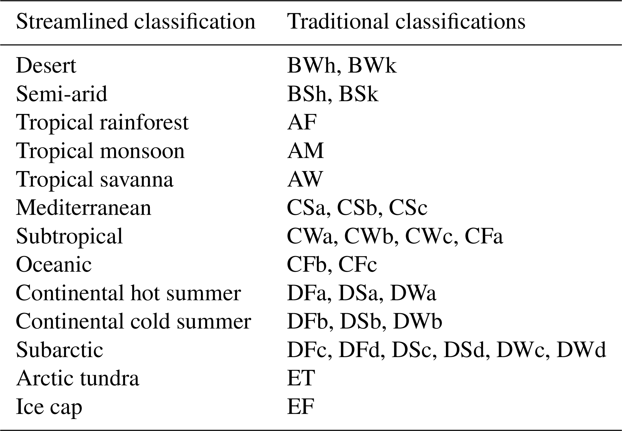
A key goal of bioclimatic classifications is to illustrate climate change in a way that is intuitive. To this end we designed a simplified Köppen–Geiger scheme that combines classifications to make changes clearer in both scale and the nature of projected transitions. Additionally, the new scheme implements a more traditional naming system. A breakdown of this streamlined system and the constituent traditional classifications involved in each of the 13 streamlined classifications is given in Table 2.
Table 2Breakdown of the streamlined classification scheme and the assignment of traditional classifications within the new scheme.
Difference maps are also plotted to demonstrate the geographical locations of major transitions between bioclimatic classifications. These difference maps plot the 10 largest transitions globally (by total land area). Areas for which less than 66 % of the models agree are hatched, demonstrating that in these regions the results are less certain.
Classification change matrices are used to quantify bioclimate transitions in terms of global land area at key levels of global warming. The columns represent the initial classification coverage, and the rows indicate the altered classification distribution. Shading highlights the size of changes in terms of the projected change as a fraction of the initial area of a given bioclimatic class.
2.2 Climate model and observational data
Historical observations of monthly mean temperature and precipitation are from the CRU TS v. 4.05 dataset (Harris et al., 2020). Analogous climate model data come from the “historical” CMIP6 experiments (Eyring et al., 2016). Models within the CMIP6 multi-model ensemble which had readily available historical experiment data and achieved a minimum of 4 K warming under the SSP585 scenario were chosen. These models are listed in Table 3.
Swart et al. (2019a)(Swart et al., 2019b)Swart et al. (2019c)(Swart et al., 2019d)Danabasoglu (2019b)(Danabasoglu, 2019a)Danabasoglu (2019c)(Danabasoglu, 2019d)Boucher et al. (2018)(Boucher et al., 2019)Tang et al. (2019)(Good et al., 2019)Dix et al. (2019a)(Dix et al., 2019b)Danek et al. (2020)(Semmler et al., 2019)Chai (2020)(Cas, 2018)EC-Earth-Consortium (2019b)(EC-Earth-Consortium, 2019a)EC-Earth-Consortium (2019d)(EC-Earth-Consortium, 2019c)Lee and Liang (2020b)(Lee and Liang, 2020a)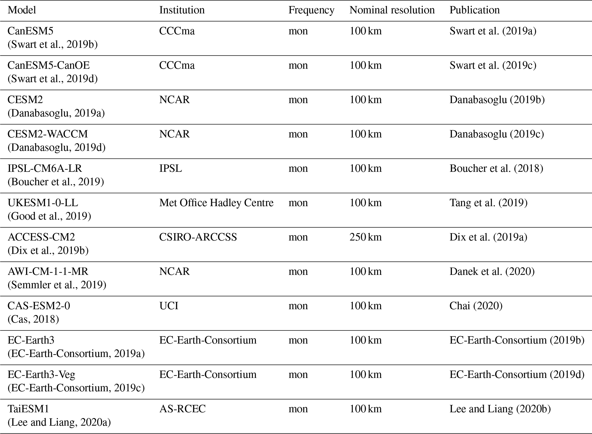
CMIP6 model data were regridded to 0.5∘ by 0.5∘, the same spatial resolution as CRU TS observations. Antarctica was excluded as observations are limited in this region, and we do not expect substantial changes in bioclimatic classification in this region.
The model output data are typically at a coarser resolution than the underlying 0.5∘ climatology. The anomaly-corrected fields therefore contain spatial variability that is solely due to the underlying climatology at scales that are not resolved by a model. This also implies that the diagnosed changes in bioclimatic types (which are dependent on the model anomalies) tend to be somewhat smoother at these finer spatial scales.
2.3 Model performance assessment
Comparison of KG observed classifications with the CMIP6 model-simulated classifications is made for the years 1901–2014. To reduce the effect of short-term variability, model and observational data are smoothed with a 30-year centred rolling mean.
The ability of individual models in the CMIP6 ensemble to simulate KG classifications of observational data during the historical period is assessed in two ways: (i) percentage land area that a model has correctly classified for each year relative to observations and (ii) percentage change in land area classification at each year compared to the initial mean 1901–1931 classifications.
2.4 Maps of KG classification versus global warming
Future KG classification maps under 1.5, 2, and 4 K of annual mean global warming above reference period levels were created from the CMIP6 “SSP585” 2015–2100 future scenario. We used SSP585 because all models pass 4 K under SSP585, which enables us to define changes in bioclimatic zones consistently for these different levels of global warming.
The timing of each warming level is found from the centred 30-year annual mean global surface air temperature above the model's reference temperature, here defined as 1901–1931. Monthly mean anomalies of precipitation and surface air temperature are calculated relative to this same reference period. Model outputs are anomaly corrected to agree with the observational over the period 1901–1931. This is done by calculating anomalies relative to that period for each model and then adding these anomalies to the observational climatology. Multi-model ensemble mean KG classification maps are calculated using the multi-model ensemble mean of the anomalous temperature and precipitation fields at each warming level. As usual in climate modelling, we focus primarily on the ensemble mean, although we note that ensemble mean and ensemble median climates have been found to be very similar (Sillmann et al., 2013; Kim et al., 2020; Li et al., 2021). These maps are hatched to indicate where models disagree on the classification. A grid point is hatched if less than 66 % of the models agree on the classification at the point.
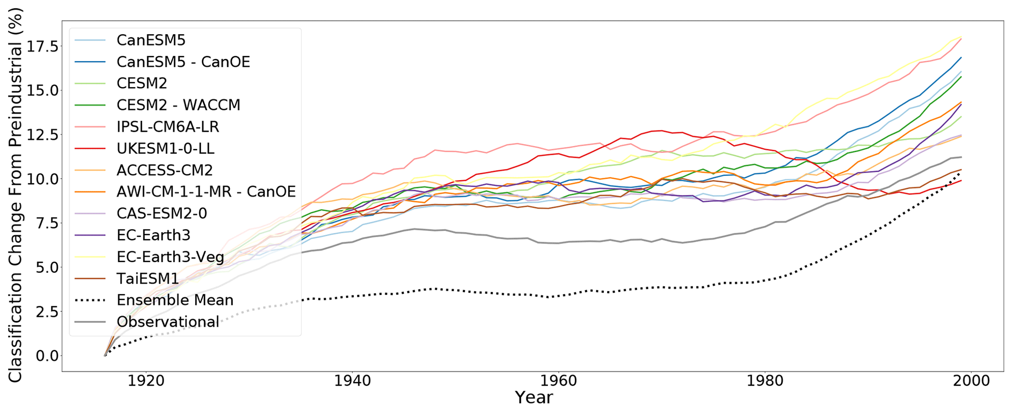
Figure 1The percentage of land area change in KG classification for each model versus year through the 20th century (without anomaly correction). The equivalent trajectory based on the observed climate is shown for comparison in dark grey. The dotted line shows the trajectory derived from the ensemble mean climate.
3.1 Model performance assessment
To gain insight into the behaviour of individual models, we create KG maps of individual models and compare these with maps derived from the observed climate. As expected, there is variation in the classification distribution of models and the observational data. For example, desertification in the Amazon is apparent in CanESM5 and CanESM5-CanOE models (Appendix A). This may show that these models have a tendency towards reduced precipitation in the tropics when compared to other models. Another area of disagreement between the models is the change in biome classification in northern Eurasia and America at various levels of global warming. The multi-model ensemble mean model state, however, reduces the effect of individual model discrepancies and compares favourably with observations.
In Fig. 1, simulated classification changes from the CMIP6 historical runs are compared to those calculated from the observed climate. The CMIP6 models broadly capture the degree of expected global classification change. All models show a similar behaviour: a large change in classifications at the start of the observed period until 1940, when the mid-century then presents an approximately constant set of classification with very little change until 1980, where again all models display further changes in climate classification. Although the multi-model ensemble mean follows the same pattern as the individual models and the observational data, it shows a lesser degree of change throughout the observed time period. This reduced variation is inherent to the nature of this ensemble mean; large changes in individual models have their impact reduced in the meaning process. This may lead to the multi-model ensemble mean displaying a similar but mitigated and delayed trend “lagging” the individual models and the observational data when creating discrete classes from climate data.
To assess the performance of individual models and their multi-model ensemble mean in classifying the bioclimate distribution according to observation-based KG for a particular year, the percentage land area correctly classified by each model every year according to observation-based KG is shown in Fig. 2. The results show that the ensemble mean is one of the best performing for classification. This is in contrast to Fig. 1, which showed that the ensemble mean was one of the worst performing for classification change. The result is also likely due to the reduced variation in data resulting from the averaging process in the creation of the multi-model ensemble mean dataset. The impact of “extreme” values present in each model are averaged out in the multi-model ensemble mean provided they are distributed around the “true” climate values. This would suggest that for individual time points, the ensemble mean is likely to provide the most reliable projection. The results from Figs. 1 and 2 give insight into the behaviour of ensemble mean datasets and when their application is appropriate. Traditionally the ensemble mean has been taken as the most likely scenario and therefore the most representative of the real-world climate. The results presented here indicate that although the ensemble mean is appropriate for assessing model output at individual points, the ensemble mean does not accurately display the variability evident in observed climate data.

3.2 Maps of KG classification versus global warming
Figure 3 shows the multi-model ensemble model mean KG classification for 1.5, 2, and 4 K of global warming above the reference period, as well as the no warming classifications. Plots for individual models for the reference period without anomaly correction and at 1, 1.5, 2, 3, and 4 K of global warming with anomaly correction are shown in Appendix A under the traditional scheme and Appendix B under the streamlined scheme. Comparison to the reference climate suggests that there could be dramatic changes in bioclimate classification, particularly in the middle to high latitudes, as the planet warms. There is less agreement in classification at the boundaries of classified regions, this is expected as the models will likely be split in classifying grid cells as one of two classifications. These changes become more apparent in Fig. 4, which uses the streamlined KG classification scheme and highlights the 10 largest bioclimatic shifts for each level of warming. Figure 4 again demonstrates less certainty at the classification change boundaries; however, the degree of agreement between the models, even at 4 K of warming, is surprisingly high.
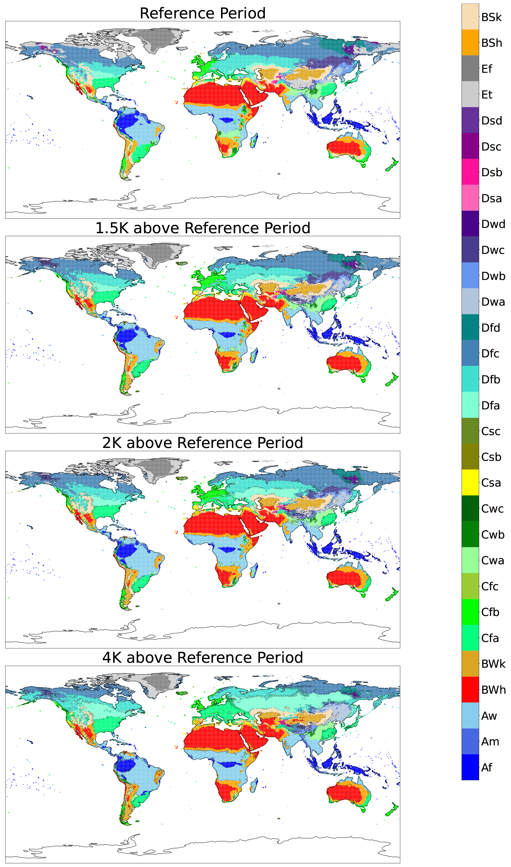
Figure 3Maps of the original KG classifications calculated from the multi-model ensemble mean for the reference period and 1.5, 2.0, and 4.0 K of global warming relative to the reference period. These were calculated from the SSP585 runs by anomaly correction relative to the observed reference climate. Hatching is present when less than 66 % of models agree on a region's classification.
These shifts are almost exclusively from wetter and colder classes to drier and hotter ones as the global temperature increases. This agrees strongly with the results found by Feng et al. (2014), which under CMIP5's RCP8.5 scenario suggested bioclimatic shifts toward warmer and drier types across the global region with climate change. Large areas undergo desertification in the Southern Hemisphere. The majority of North America and northern Eurasia has a shift towards warmer climates as subarctic gives way to continental cold summer, and continental cold summer is replaced by continental warm summer. All changes in classification with the streamlined KG scheme are quantified in Fig. 5. Although the KG scheme exclusively maps climate, the biologic implications of these changes can be seen. The subarctic region has historically been dominated by the boreal forest (Kayes and Mallik, 2020), though there is evidence suggesting a slow northward migration of non-native warmth-adapted tree species into historically boreal areas (Viacheslav et al., 2007; Boisvert-Marsh et al., 2014). However, the rate of global warming far exceeds the rate of boreal migration due to limits on the tree's ability to migrate (McKenney et al., 2007). With the continued reduction in the subarctic bioclimate we predict a likely continuation of these trends. The indicated shift in the Amazon from tropical rainforest to savanna can also be seen; an expansion of white-sand savannas in the Amazon has already been found (Flo and Holmgren, 2021).
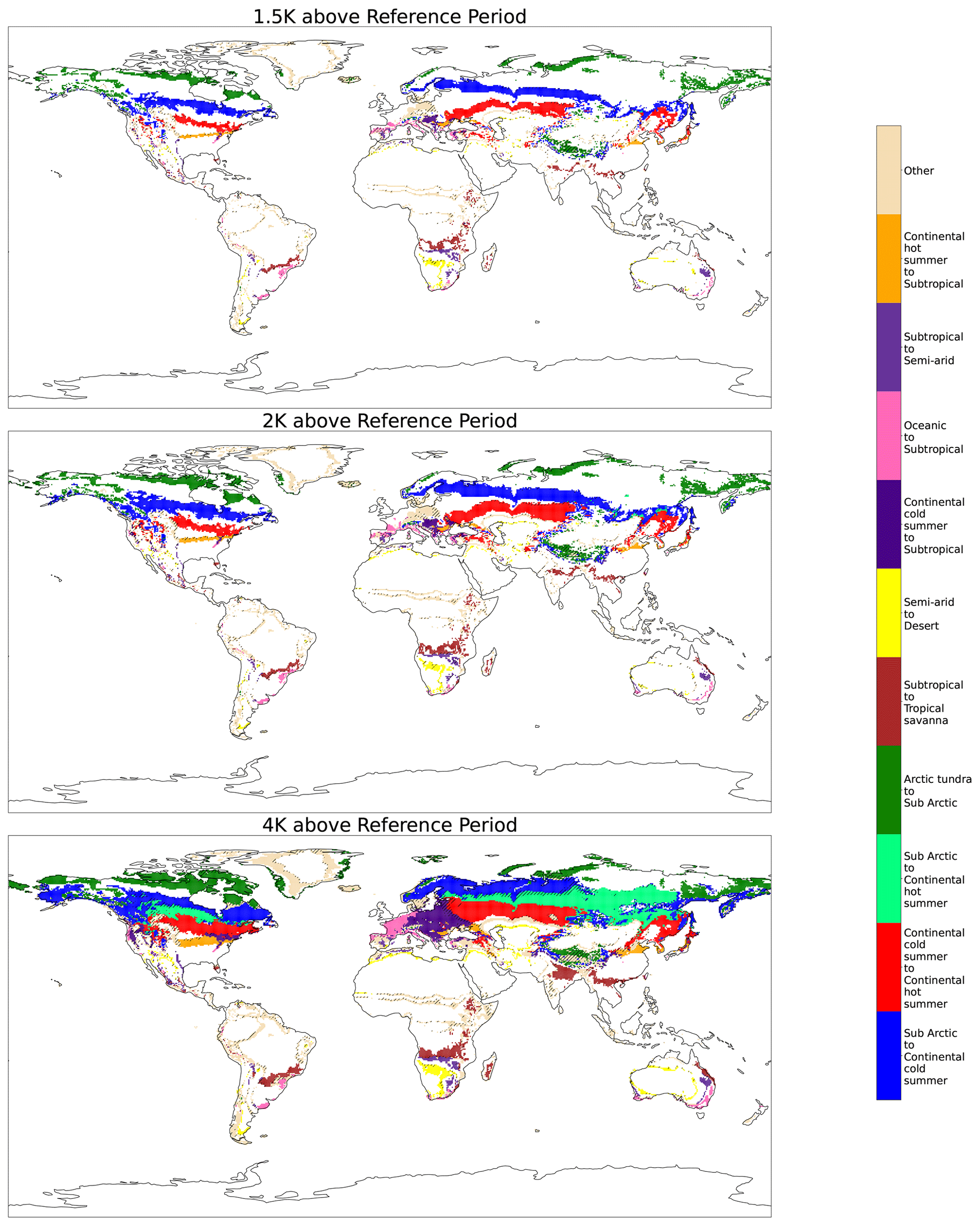
Figure 4Multi-model ensemble mean difference maps highlighting the 10 largest classification changes for 4 K of warming above the reference period using the streamlined classification system. Hatching is present when less than 66 % of models agree on a region's classification change.
At 4 K areas of classification change represent over 33 % of land area. The change in percentage of total land area in Fig. 5c gives some alarming perspectives; for example, at +4 K arctic tundra is indicated to cover over 25 % less land area than in the reference period. At 2 K the models already project substantial changes to the global distribution of bioclimates; at 4 K these changes become even more pronounced.
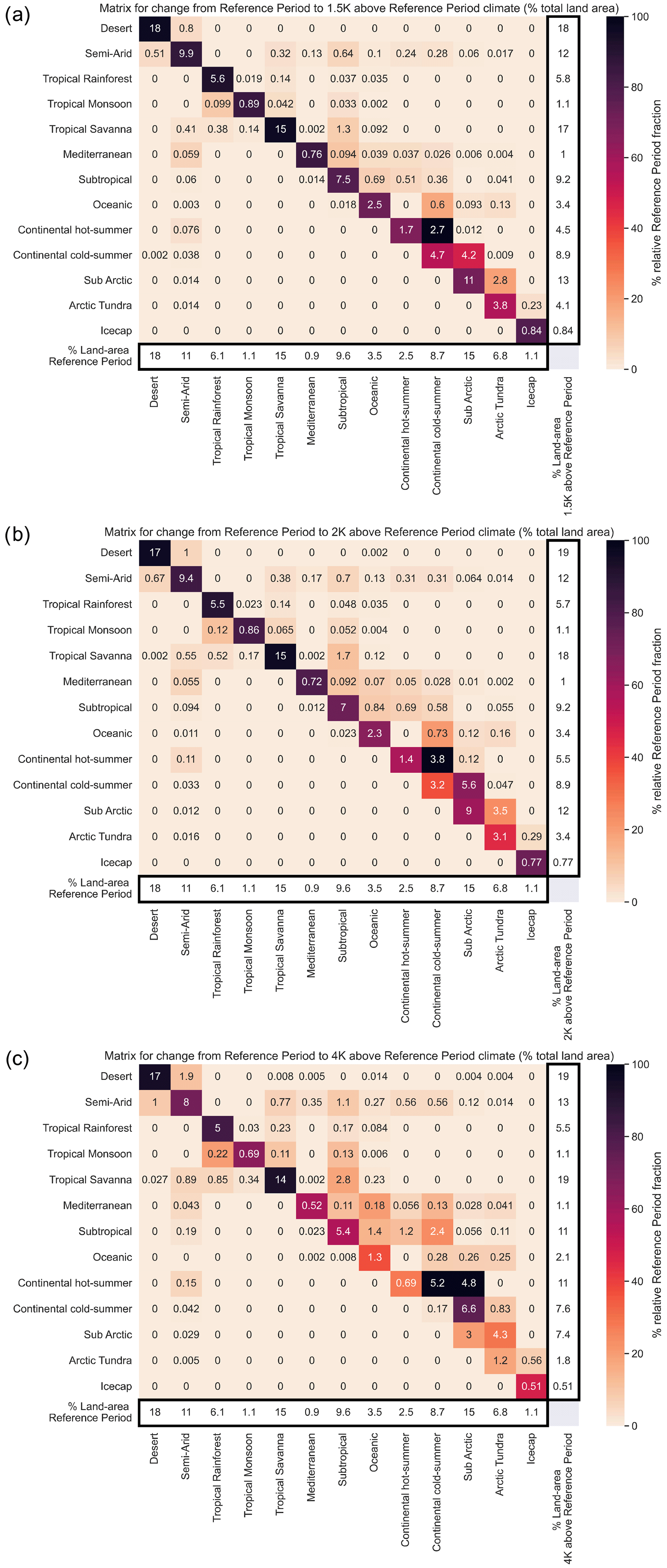
Figure 5Multi-model ensemble mean difference matrices highlighting the classification changes for levels of warming above the reference period of (a) 1.5 K, (b) 2 K, and (c) 4 K using the streamlined classification system.
Table 4Percentage change in the global land area of each of the streamlined classifications per degree of global warming. Change is based on linear approximations of results from reference period to 4 K of warming.
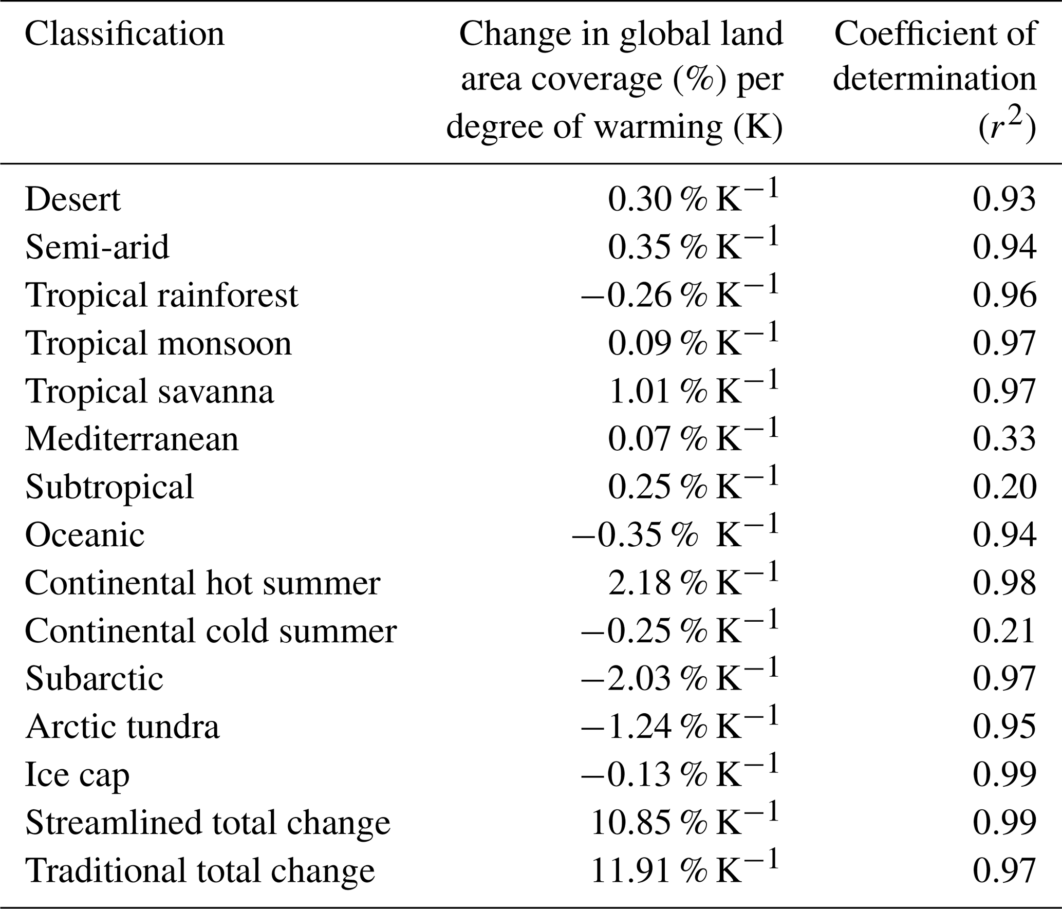
In Table 4 we give the percentage change in global land area of each of the streamlined classifications per degree of warming assuming the dependence is linear up to 4 K of warming. Linear dependence is a good approximation for most classifications with all but three having r2>0.9. The three poorly fitting classifications, those for Mediterranean, subtropical, and continental cold-summer bioclimates, may be transitory classifications whose peak or minimum land area coverage is within the 4 K range the linear equation is based on. Classifications predicted to decrease in global fraction under global warming (with good r2) are tropical rainforest, oceanic, subarctic, arctic tundra, and ice cap, the largest decrease of which globally is subarctic (2.03 % K−1). Classifications that increase under global warming with good certainty are desert, semi-arid, tropical monsoon, tropical savanna and continental hot-summer with the largest increase predicted to be continental hot-summer (2.18 % K−1). Raw plots for these fits without lines fitted can be found in Appendix C.
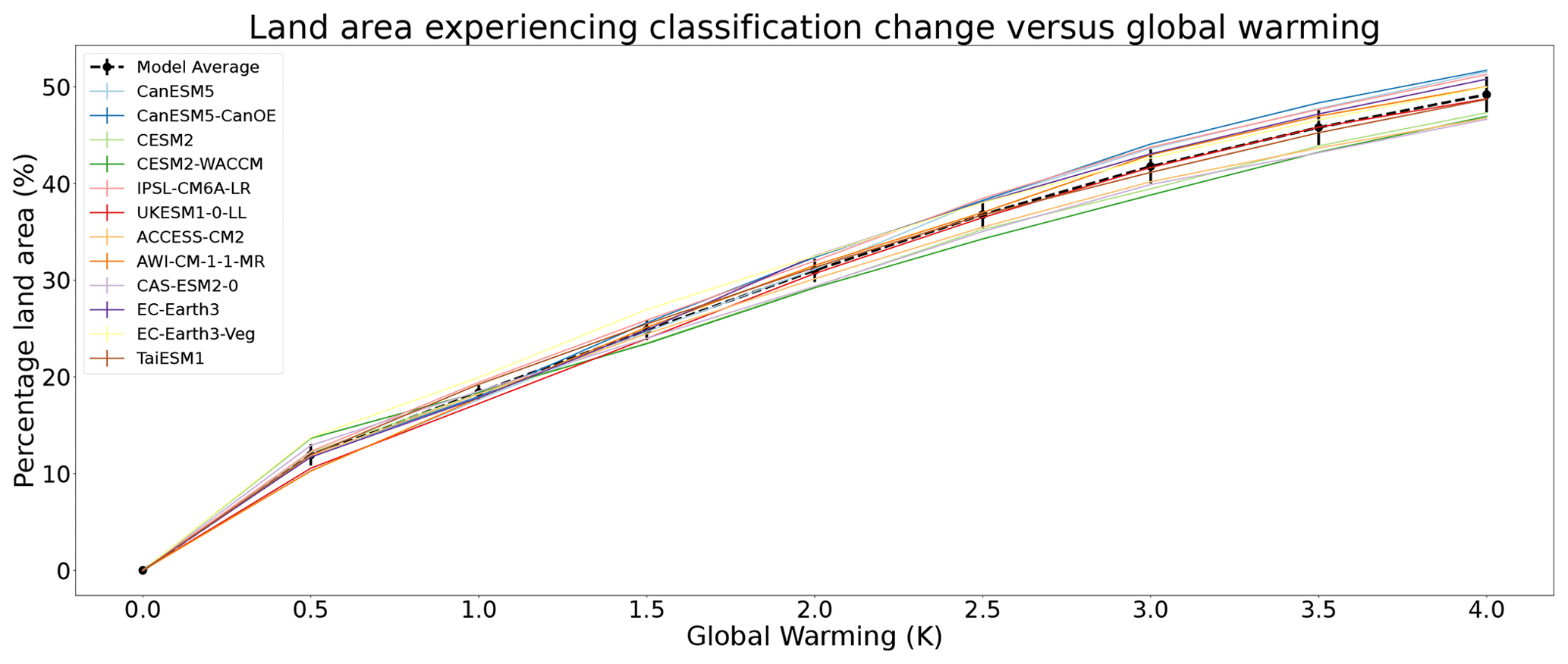
Figure 6The percentage of land area projected to see a change in bioclimate as a function of global warming, using the traditional Köppen–Geiger classification with anomaly correction. Note the robust agreement between models, which implies a multi-model ensemble mean change which is well approximated by .
3.3 Sensitivity of bioclimate to global warming
Figure 6 displays a weakly saturating increase with global warming, the fraction of land area that experiences a change in classification follows Eq. (1):
where f is the fraction of land area that experiences a change in bioclimatic classification, ΔT is the global warming relative to the reference period climate, and k is a fitting parameter. The mean response across the models suggests a value of k∼0.14 K−1. This was calculated to have a coefficient of determination of 0.84. For the range of global warming of particular interest to the Paris Climate Agreement (1 to 3∘C of warming) the land area experiencing a change in bioclimatic classification is approximately 13 % of the global land per kelvin of global warming. The total land area (neglecting Antarctica) is approximately 146 million square kilometres, so this implies a bioclimatic change for 18.9 million square kilometres of land per degree of warming between 1 and 3 K. This highlights the benefits of keeping global warming to 1.5 K as opposed to 2 K of warming, as the 0.5 K difference represents an additional bioclimatic change for over 7.5 million square kilometres of land. These bioclimatic changes being increases of 1 % in land area of desert, tropical savanna, and continental hot summer biomes. Subarctic and arctic tundra decrease by 1 and 0.7 % respectively. Between 1.5 and 2 K there are relatively small or no changes between the remaining classifications in Fig. 5a, b.
Previous studies of classification change with global warming have been regional, studies such as Kim and Bae (2021) suggest a classification area change of approximately 15 % of Asian monsoon regions at 2 K of warming. However, regional assessments at the Equator or in the Southern Hemisphere are likely to under-represent global changes in classification, as the majority of classification change is predicted to be north of 30∘ N (Feng et al., 2014). A quantitative distribution of climate classification changes between global warming levels of 1.5 and 2 K can be seen in Appendix C (note that this breakdown uses the streamlined KG system and subsequently will not represent all changes included in Fig. 6).
Despite the difference in climate projections for given greenhouse gas emissions, we present strong evidence that climate models agree well on the extent of bioclimatic change the global land surface will undergo per degree of global warming. The Köppen–Geiger scheme has been used to present the impact of global warming at 1.5, 2, and 4 K of warming above reference period levels in the form of climate maps, showing the global distribution of bioclimates, and as graphs and classification change matrices at various levels of warming.
Bioclimate classifications are fundamentally climate classifiers, but they are designed to represent and correlate with biome distribution. In this way the warming maps and classification changes represent tangible shifts in the global distribution of ecosystems, giving insight into the nature of Earth at various levels of warming. This paper also uses the Köppen–Geiger scheme as a method for climate model verification that is relevant to the impacts of climate change on ecosystems. The Köppen–Geiger maps at levels of global warming demonstrate the impact that climate change could have. The transition matrices present an easily interpretable method for understanding and quantifying the scale of all classification changes. The results presented by the maps and matrices predict large changes in global bioclimate distribution, with hotter, drier bioclimates expanding and colder, wetter bioclimates shrinking and moving further towards the poles.
The combination of the techniques presented in this paper indicate that the impact of global warming on KG bioclimates is roughly linear for levels of warming between 1 and 3 K. We find that 13 % of land could experience a substantial change in bioclimate per degree Celsius of global warming.
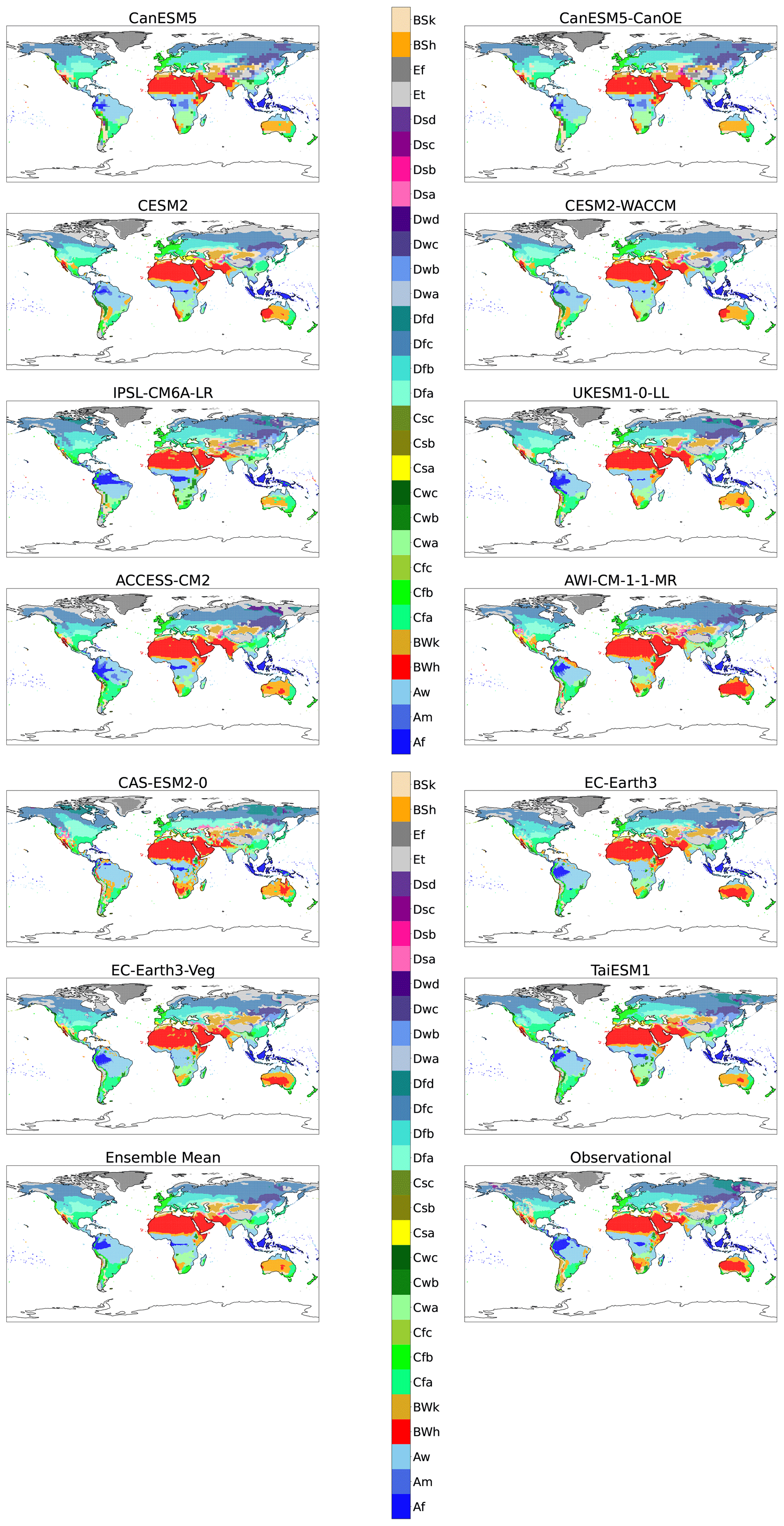
Figure A1Maps of KG classifications for each model for the reference period (1901–1931) without anomaly correction.

Figure A2Maps of KG classifications for each model at +1 K with anomaly correction.
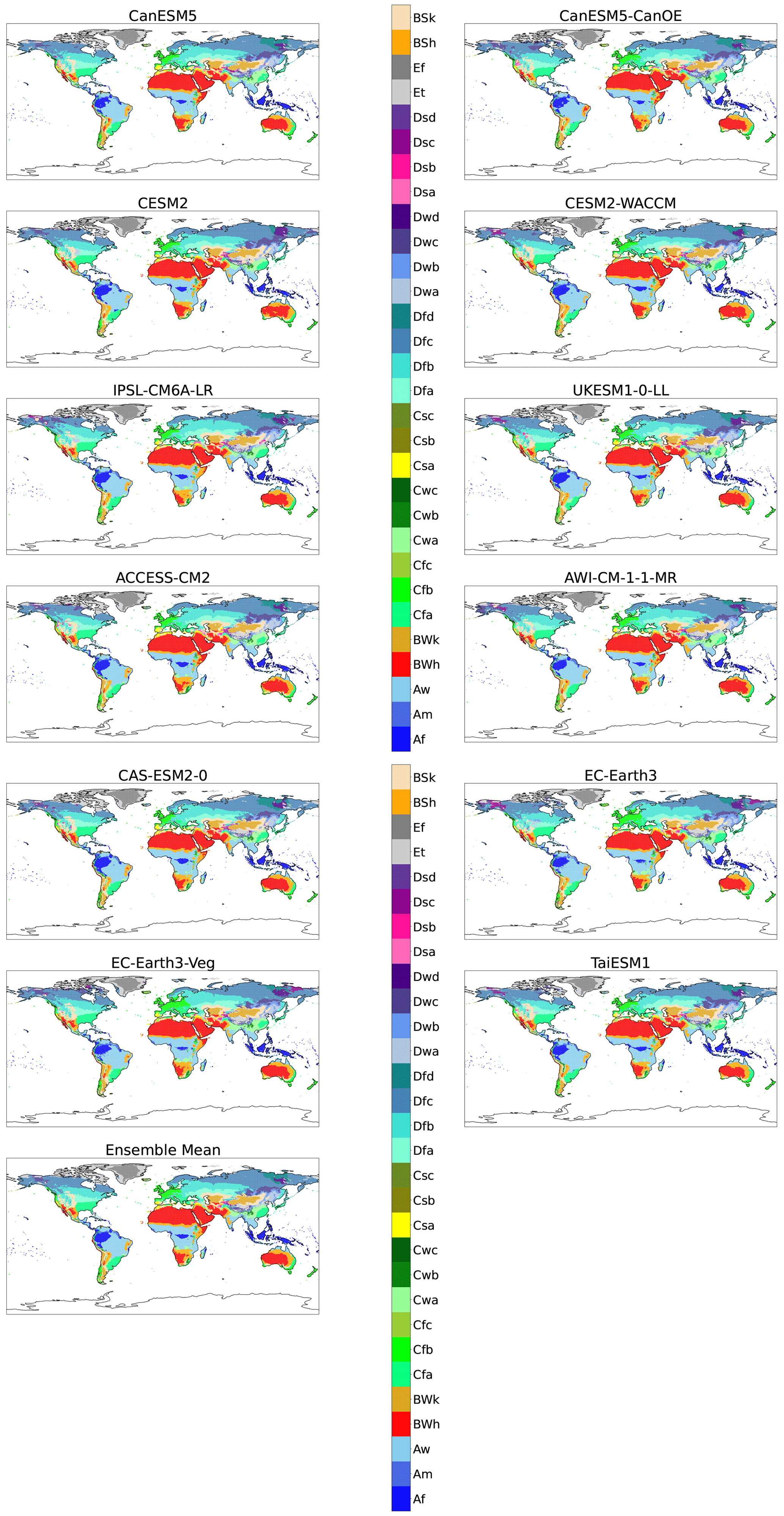
Figure A3Maps of KG classifications for each model at +1.5 K with anomaly correction.
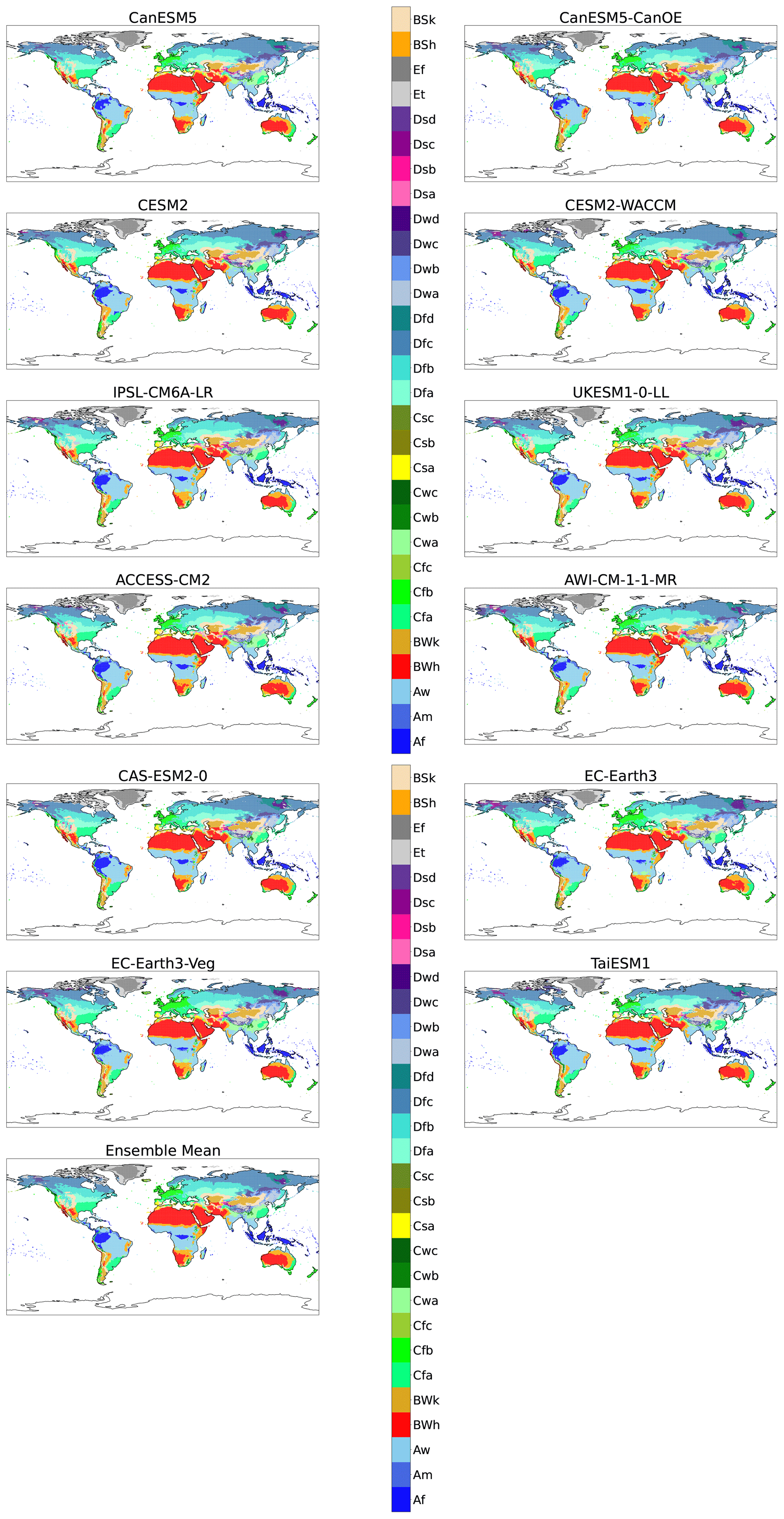
Figure A4Maps of KG classifications for each model at +2 K with anomaly correction.

Figure A5Maps of KG classifications for each model at +3 K with anomaly correction.
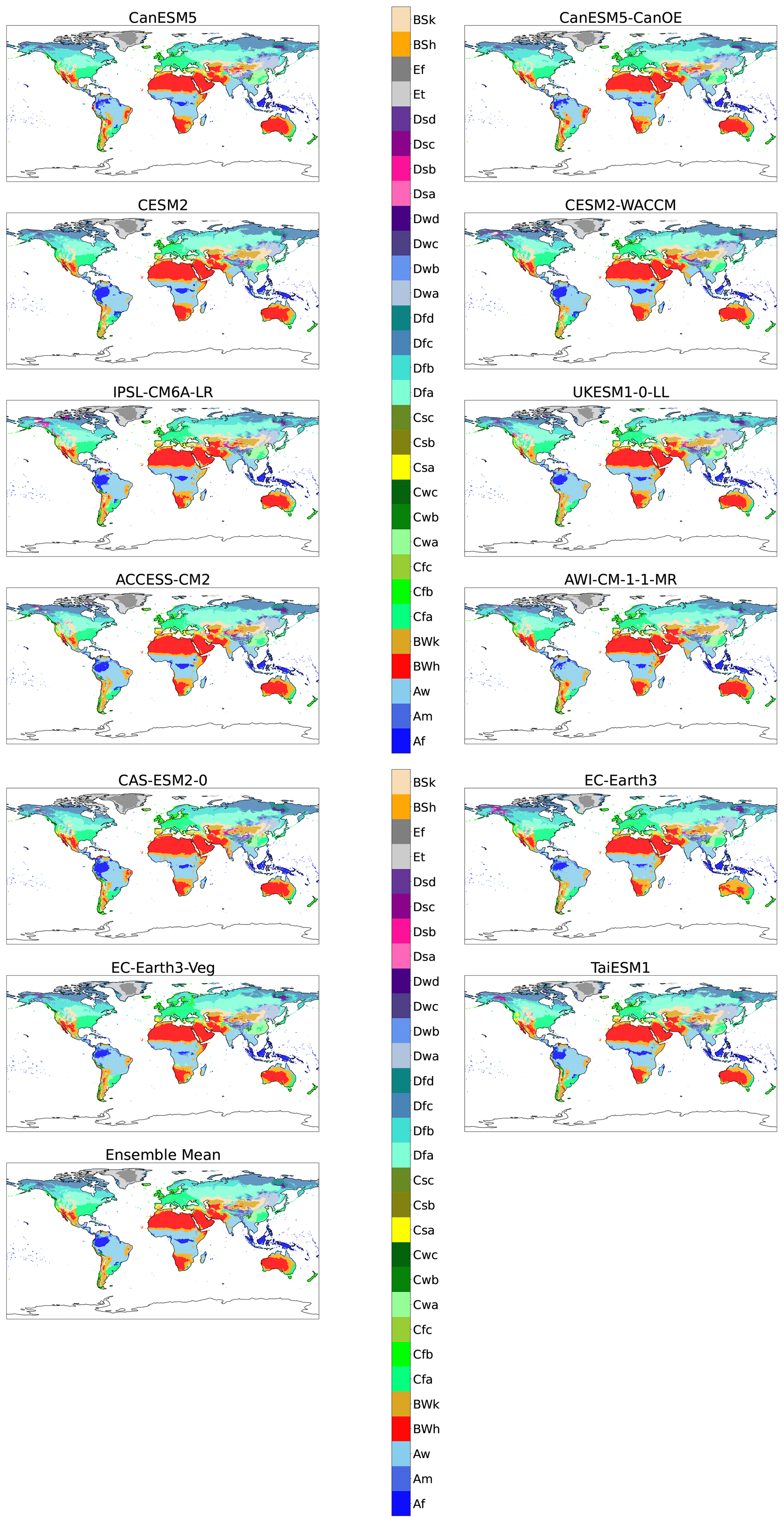
Figure A6Maps of KG classifications for each model at +4 K with anomaly correction.
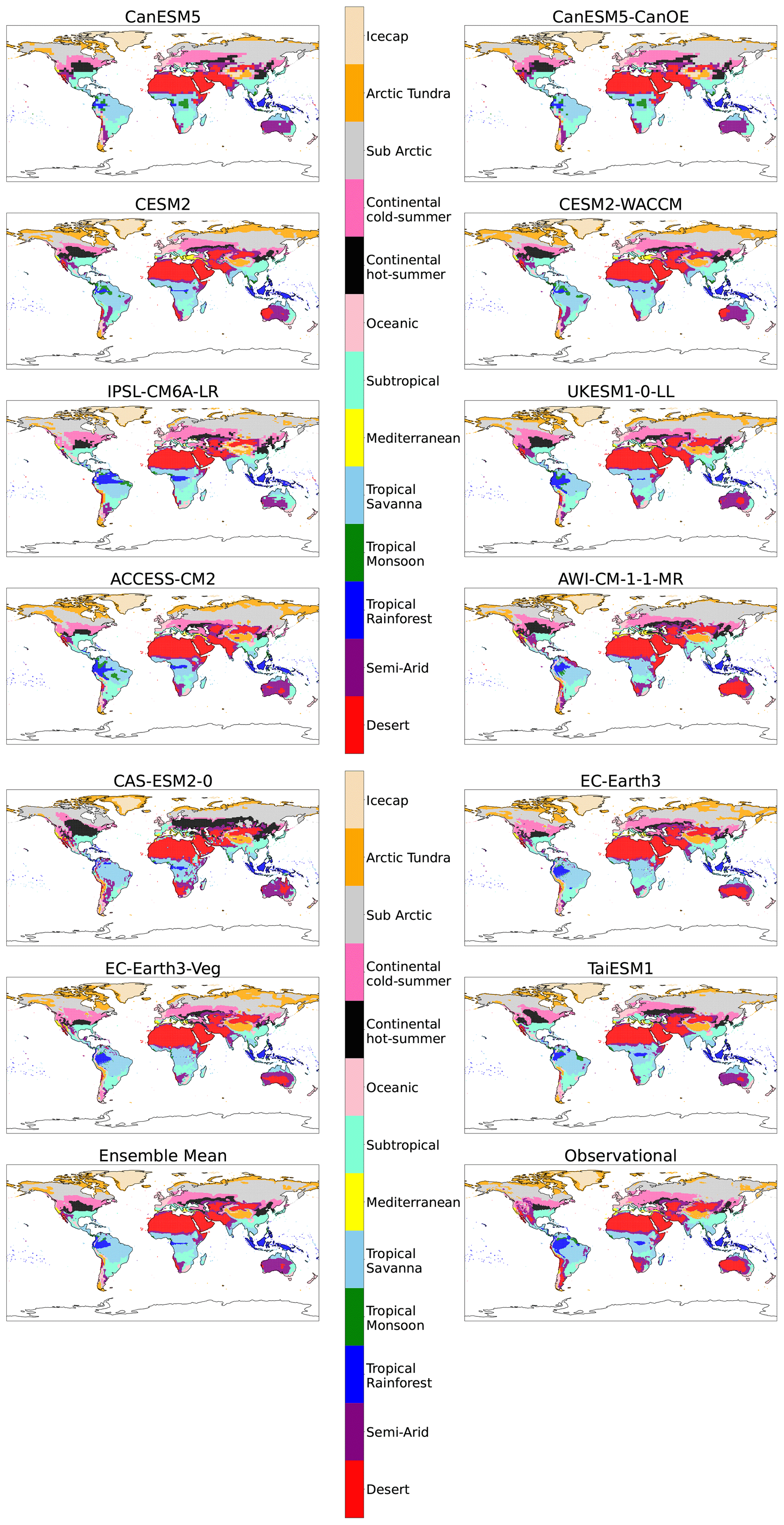
Figure B1Maps of streamlined KG classifications for each model for the reference period (1901–1931) without anomaly correction.

Figure B2Maps of streamlined KG classifications for each model at +1 K with anomaly correction.
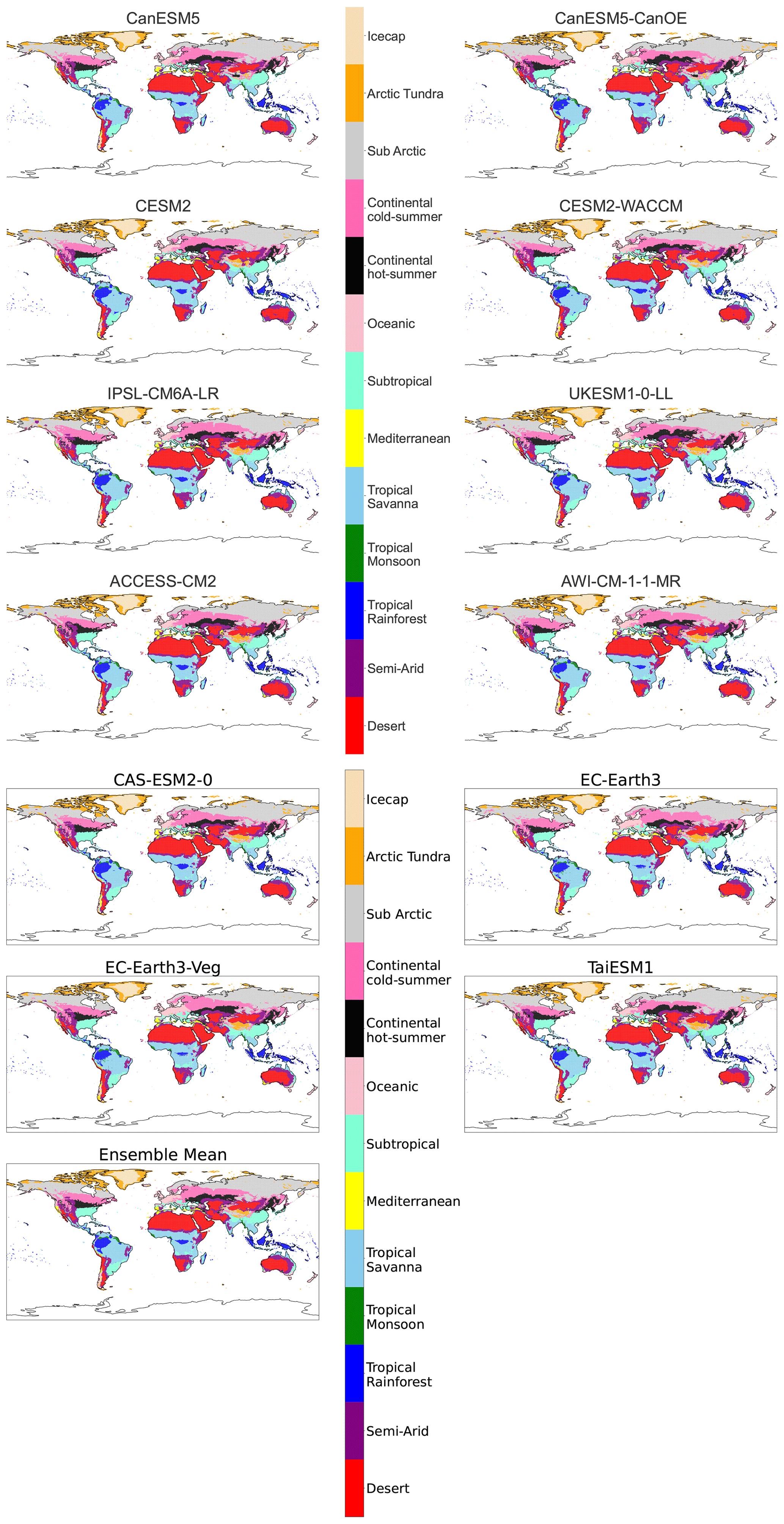
Figure B3Maps of streamlined KG classifications for each model at +1.5 K with anomaly correction.
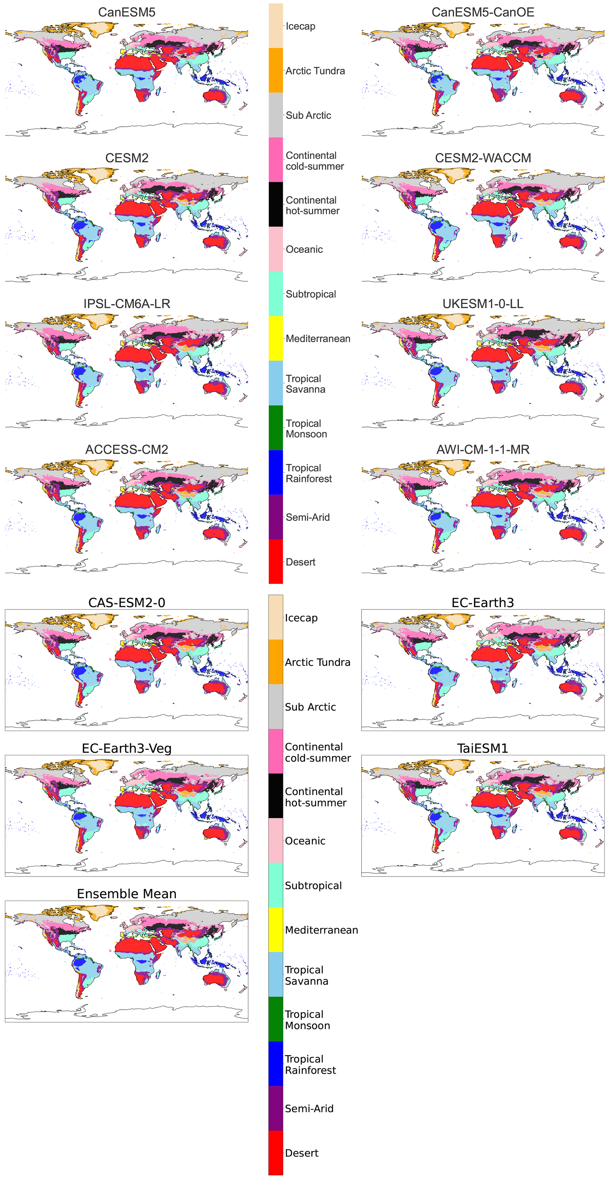
Figure B4Maps of streamlined KG classifications for each model at +2 K with anomaly correction.
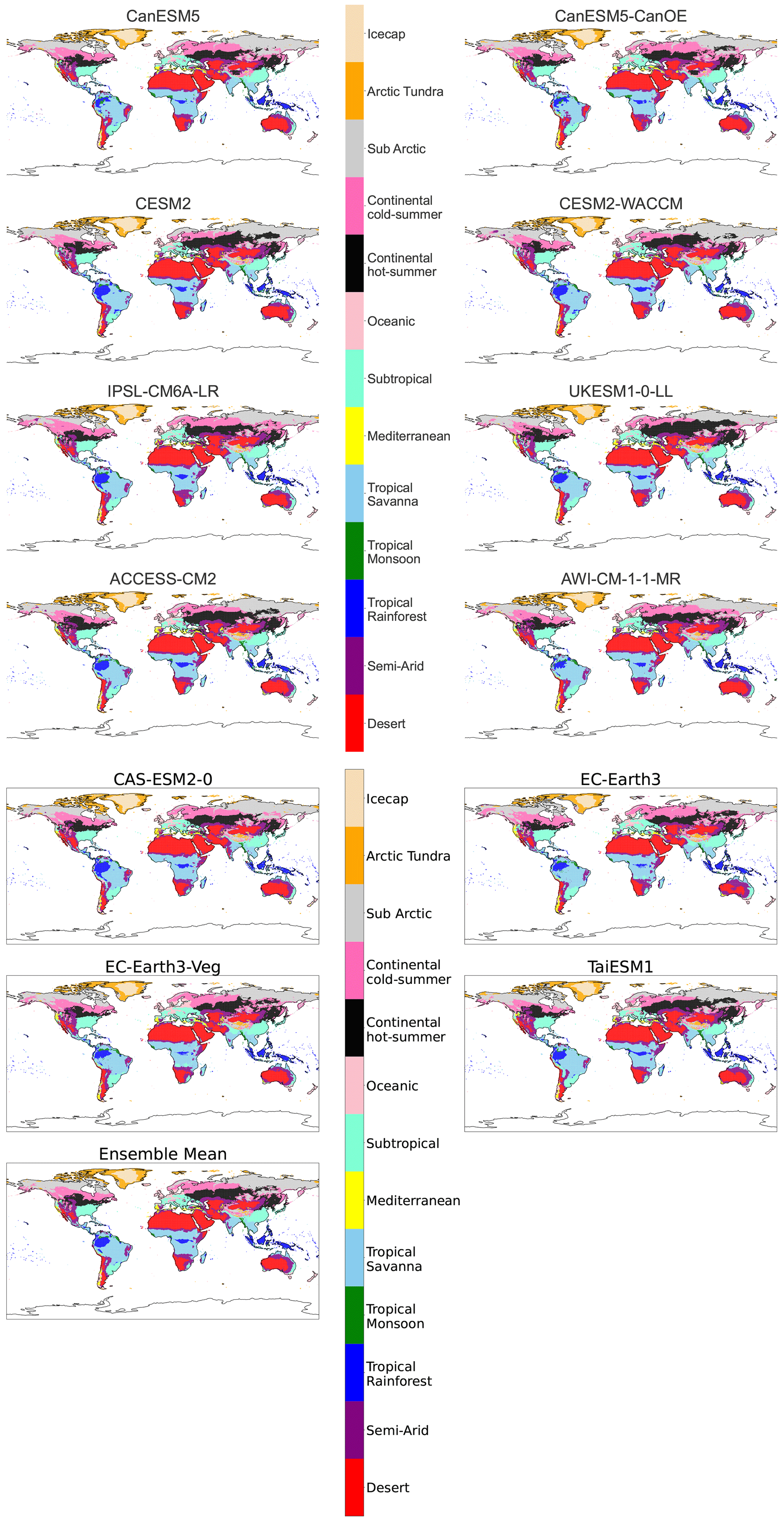
Figure B5Maps of streamlined KG classifications for each model at +3 K with anomaly correction.
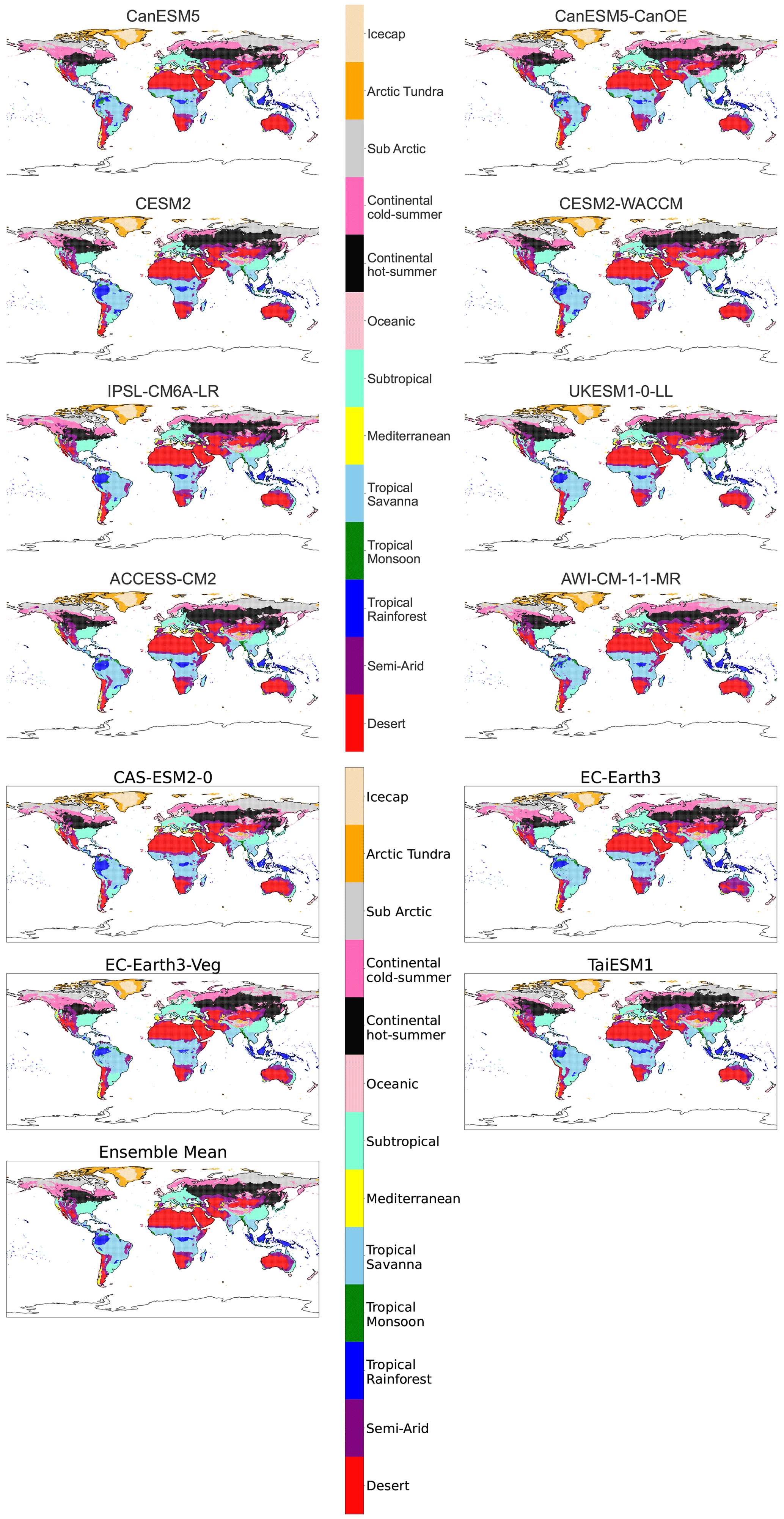
Figure B6Maps of streamlined KG classifications for each model at +4 K with anomaly correction.
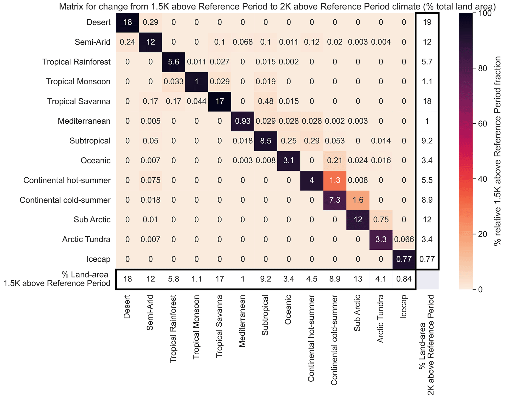
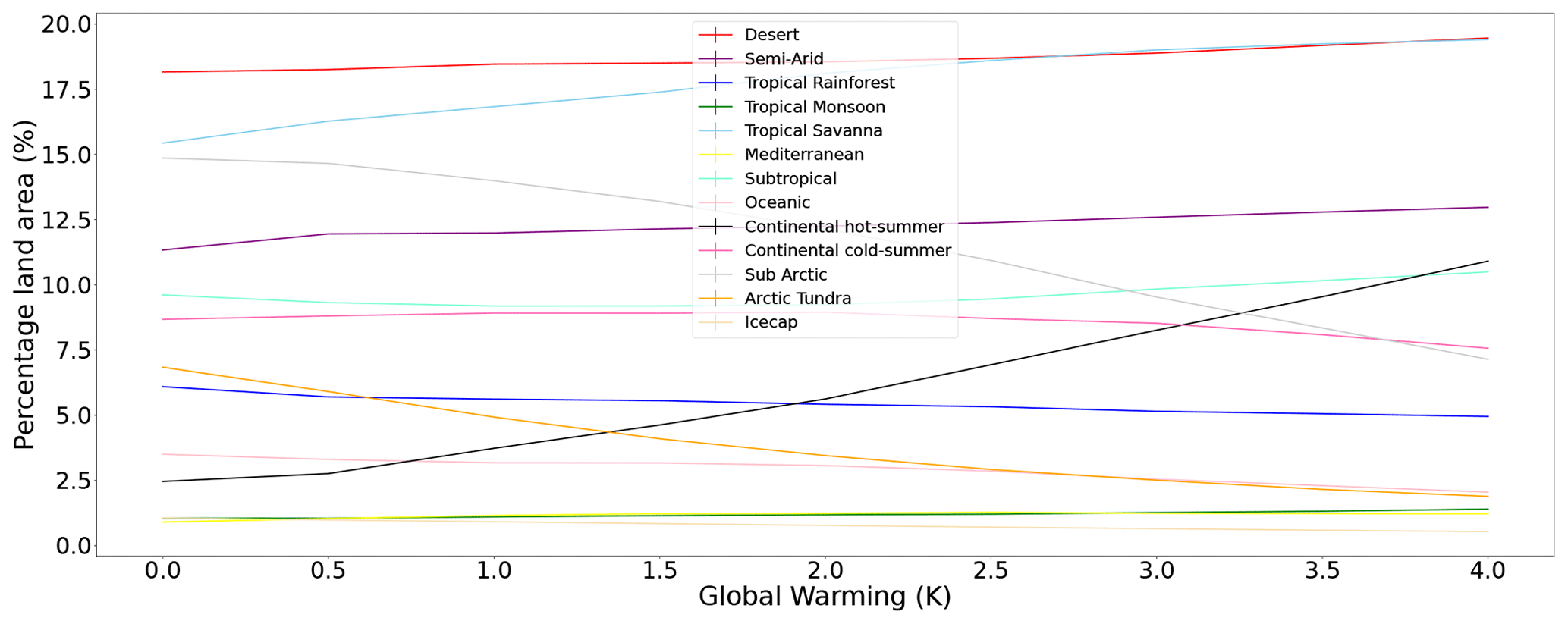
Figure D1Land area distribution of individual streamlined classifications. Classifications that show large growth in their coverage include continental hot summer and tropical savanna. Classifications that show major reductions include ice cap, arctic tundra, and subarctic.
Based on publicly available CMIP6 data (doi10.5194/gmd-9-1937-2016, Eyring et al., 2016).
MS carried out the data analysis and drafted the paper. MSW and PC advised on the study. All authors contributed to the submitted paper.
The contact author has declared that none of the authors has any competing interests.
Publisher's note: Copernicus Publications remains neutral with regard to jurisdictional claims in published maps and institutional affiliations.
We acknowledge the World Climate Research Programme's Working Group on Coupled Modelling, which is responsible for CMIP, and we thank the climate modelling groups for producing and making available model output from the CMIP6 models.
This research has been supported by the European Research Council “Emergent Constraints on Climate-Land feedbacks in the Earth System (ECCLES)” project under the grant no. 742472 (Mark S. Williamson and Peter M. Cox). Peter M. Cox was also supported by the European Union's Framework Programme Horizon 2020 for Research and Innovation under grant agreement no. 821003, Climate–Carbon Interactions in the Current Century (4C) project.
This paper was edited by Martin De Kauwe and reviewed by three anonymous referees.
Argles, A. P. K., Moore, J. R., and Cox, P. M.: Dynamic Global Vegetation Models: Searching for the balance between demographic process representation and computational tractability, PLOS Climate, 1, 1–18, https://doi.org/10.1371/journal.pclm.0000068, 2022. a
Beck, H. E., Zimmermann, N. E., McVicar, T. R., Vergopolan, N., Berg, A., and Wood, E. F.: Present and future Köppen-Geiger climate classification maps at 1-km resolution, Sci. Data, 5, 180214, https://doi.org/10.1038/sdata.2018.214, 2018. a, b
Boisvert-Marsh, L., Périé, C., and Blois, S. D.: Shifting with climate? Evidence for recent changes in tree species distribution at high latitudes, Ecosphere, 5, 23, https://doi.org/10.1890/ES14-00111.1, 2014. a
Boucher, O., Denvil, S., Levavasseur, G., Cozic, A., Caubel, A., Foujols, M.-A., Meurdesoif, Y., Cadule, P., Devilliers, M., Ghattas, J., Lebas, N., Lurton, T., Mellul, L., Musat, I., Mignot, J., and Cheruy, F.: IPSL IPSL-CM6A-LR model output prepared for CMIP6 CMIP historical, https://doi.org/10.22033/ESGF/CMIP6.5195, 2018. a
Boucher, O., Denvil, S., Levavasseur, G., Cozic, A., Caubel, A., Foujols, M.-A., Meurdesoif, Y., Cadule, P., Devilliers, M., Dupont, E., and Lurton, T.: IPSL IPSL-CM6A-LR model output prepared for CMIP6 ScenarioMIP ssp585, https://doi.org/10.22033/ESGF/CMIP6.5271, 2019. a
CAS CAS-ESM1.0 model output prepared for CMIP6 ScenarioMIP ssp585, http://cera-www.dkrz.de/WDCC/meta/CMIP6/CMIP6.ScenarioMIP.CAS.CAS-ESM2-0.ssp585 (last access: 23 January 2023), 2018. a
Chai, Z.: CAS CAS-ESM1.0 model output prepared for CMIP6 CMIP historical, https://doi.org/10.22033/ESGF/CMIP6.3353, 2020. a
Cox, P., Huntingford, C., Nuttall, P., and Sparey, M.: Climate, Ticks and Disease, CABI, https://doi.org/10.1079/9781789249637.0003, 2021. a
Danabasoglu, G.: NCAR CESM2 model output prepared for CMIP6 ScenarioMIP ssp585, https://doi.org/10.22033/ESGF/CMIP6.7768, 2019a. a
Danabasoglu, G.: NCAR CESM2 model output prepared for CMIP6 CMIP historical, https://doi.org/10.22033/ESGF/CMIP6.7627, 2019b. a
Danabasoglu, G.: NCAR CESM2-WACCM model output prepared for CMIP6 CMIP historical, https://doi.org/10.22033/ESGF/CMIP6.10071, 2019c. a
Danabasoglu, G.: NCAR CESM2-WACCM model output prepared for CMIP6 ScenarioMIP ssp585, https://doi.org/10.22033/ESGF/CMIP6.10115, 2019d. a
Danek, C., Shi, X., Stepanek, C., Yang, H., Barbi, D., Hegewald, J., and Lohmann, G.: AWI AWI-ESM1.1LR model output prepared for CMIP6 CMIP historical, https://doi.org/10.22033/ESGF/CMIP6.9328, 2020. a
Dix, M., Bi, D., Dobrohotoff, P., Fiedler, R., Harman, I., Law, R., Mackallah, C., Marsland, S., O'Farrell, S., Rashid, H., Srbinovsky, J., Sullivan, A., Trenham, C., Vohralik, P., Watterson, I., Williams, G., Woodhouse, M., Bodman, R., Dias, F. B., Domingues, C. M., Hannah, N., Heerdegen, A., Savita, A., Wales, S., Allen, C., Druken, K., Evans, B., Richards, C., Ridzwan, S. M., Roberts, D., Smillie, J., Snow, K., Ward, M., and Yang, R.: CSIRO-ARCCSS ACCESS-CM2 model output prepared for CMIP6 CMIP historical, https://doi.org/10.22033/ESGF/CMIP6.4271, 2019a. a
Dix, M., Bi, D., Dobrohotoff, P., Fiedler, R., Harman, I., Law, R., Mackallah, C., Marsland, S., O'Farrell, S., Rashid, H., Srbinovsky, J., Sullivan, A., Trenham, C., Vohralik, P., Watterson, I., Williams, G., Woodhouse, M., Bodman, R., Dias, F. B., Domingues, C. M., Hannah, N., Heerdegen, A., Savita, A., Wales, S., Allen, C., Druken, K., Evans, B., Richards, C., Ridzwan, S. M., Roberts, D., Smillie, J., Snow, K., Ward, M., and Yang, R.: CSIRO-ARCCSS ACCESS-CM2 model output prepared for CMIP6 ScenarioMIP ssp585, https://doi.org/10.22033/ESGF/CMIP6.4332, 2019b. a
EC-Earth-Consortium: EC-Earth-Consortium EC-Earth3 model output prepared for CMIP6 ScenarioMIP ssp585, https://doi.org/10.22033/ESGF/CMIP6.4912, 2019a. a
EC-Earth-Consortium: EC-Earth-Consortium EC-Earth3 model output prepared for CMIP6 CMIP historical, https://doi.org/10.22033/ESGF/CMIP6.4700, 2019b. a
EC-Earth-Consortium: EC-Earth-Consortium EC-Earth3-Veg model output prepared for CMIP6 ScenarioMIP ssp585, https://doi.org/10.22033/ESGF/CMIP6.4914, 2019c. a
EC-Earth-Consortium: EC-Earth-Consortium EC-Earth3-Veg model output prepared for CMIP6 CMIP historical, https://doi.org/10.22033/ESGF/CMIP6.4706, 2019d. a
Every, J. P., Li, L., and Dorrell, D. G.: Köppen-Geiger climate classification adjustment of the BRL diffuse irradiation model for Australian locations, Renew. Energ., 147, 2453–2469, https://doi.org/10.1016/j.renene.2019.09.114, 2020. a
Eyring, V., Bony, S., Meehl, G. A., Senior, C. A., Stevens, B., Stouffer, R. J., and Taylor, K. E.: Overview of the Coupled Model Intercomparison Project Phase 6 (CMIP6) experimental design and organization, [data set], Geosci. Model Dev., 9, 1937–1958, https://doi.org/10.5194/gmd-9-1937-2016, 2016. a, b, c
Feng, S., Hu, Q., Huang, W., Ho, C.-H., Li, R., and Tang, Z.: Projected climate regime shift under future global warming from multi-model, multi-scenario CMIP5 simulations, Global Planet. Change, 112, 41–52, https://doi.org/10.1016/j.gloplacha.2013.11.002, 2014. a, b
Flores, B. M. and Holmgren, M.: White-Sand Savannas Expand at the Core of the Amazon After Forest Wildfires, Ecosystems, 24, 1624–1637, https://doi.org/10.1007/s10021-021-0060, 2021. a
Good, P., Sellar, A., Tang, Y., Rumbold, S., Ellis, R., Kelley, D., and Kuhlbrodt, T.: MOHC UKESM1.0-LL model output prepared for CMIP6 ScenarioMIP ssp585, https://doi.org/10.22033/ESGF/CMIP6.6405, 2019. a
Harris, I., Osborn, T., Jones, P., and Lister, D.: Version 4 of the CRU TS monthly high-resolution gridded multivariate climate dataset, Sci. Data, 7, 109, https://doi.org/10.1038/s41597-020-0453-3, 2020. a
Kayes, I. and Mallik, A.: Boreal Forests: Distributions, Biodiversity, and Management, Part of the Encyclopedia of the UN Sustainable Development Goals book series (ENUNSDG), https://doi.org/10.1007/978-3-319-71065-5_17-1, 2020. a
Kim, J.-B. and Bae, D.-H.: The Impacts of Global Warming on Climate Zone Changes Over Asia Based on CMIP6 Projections, Earth Space Sci., 8, e2021EA001701, https://doi.org/10.1029/2021EA001701, 2021. a, b
Kim, Y. H., Min, S. K., Zhang, X., Sillmann, J., and Sandstad, M.: Evaluation of the CMIP6 multi-model ensemble for climate extreme indices, Weather Clim. Ext., 29, 100269, https://doi.org/10.1016/j.wace.2020.100269, 2020. a
Kottek, M., Grieser, J., Beck, C., Rudolf, B., and Rubel, F.: World Map of the Köppen-Geiger Climate Classification Updated, Meteorol. Z., 15, 259–263, https://doi.org/10.1127/0941-2948/2006/0130, 2006. a
Köppen, W.: Die Wärmezonen der Erde, nach der Dauer der heissen, gemässigten und kalten Zeit und nach der Wirkung der Wärme auf die organische Welt betrachtet, Meteorol. Z., 1, 215–226, https://doi.org/10.1007/s11367-013-0693-y, 1884. a
Köppen, W.: Das geographische System der Klimate,, Gebrüder Borntraeger, 1–44, 1936. a
Lee, W.-L. and Liang, H.-C.: AS-RCEC TaiESM1.0 model output prepared for CMIP6 ScenarioMIP ssp585, https://doi.org/10.22033/ESGF/CMIP6.9823, 2020a. a
Lee, W.-L. and Liang, H.-C.: AS-RCEC TaiESM1.0 model output prepared for CMIP6 CMIP historical, https://doi.org/10.22033/ESGF/CMIP6.9755, 2020b. a
Li, J., Miao, C., Wei, W., Zhang, G., Hua, L., Chen, Y., and Wang, X.: Evaluation of CMIP6 Global Climate Models for Simulating Land Surface Energy and Water Fluxes During 1979–2014, J. Adv. Model. Earth Sy., 13, e2021MS002515, https://doi.org/10.1029/2021MS002515, 2021. a
Lugo, A. E., Brown, S. L., Dodson, R., Smith, T. S., and Shugart, H. H.: The Holdridge life zones of the conterminous United States in relation to ecosystem mapping, J. Biogeogr., 26, 1025–1038, https://doi.org/10.1046/j.1365-2699.1999.00329.x, 1999. a
Masson-Delmotte, V., Zhai, P., Pirani, A., Connors, S., Péan, C., Berger, S., Caud, N., Chen, Y., Goldfarb, L., Gomis, M., Huang, M., Leitzell, K., Lonnoy, E., Matthews, J., Maycock, T., Waterfield, T., Yelekçi, O., Yu, R., and Zhou, B. E.: Summary for Policymakers, in: Climate Change 2021: The Physical Science Basis, Contribution of Working Group I to the Sixth Assessment Report of the Intergovernmental Panel on Climate Change, IPCC, Cambridge University Press., https://doi.org/10.1017/9781009157896, 2021. a
McKenney, D. W., Pedlar, J. H., Lawrence, K., Campbell, K., and Hutchinson, M. F.: Potential Impacts of Climate Change on the Distribution of North American Trees, Bioscience, 57, 939–948, https://doi.org/10.1641/B571106, 2007. a
Nijsse, F. J. M. M., Cox, P. M., and Williamson, M. S.: Emergent constraints on transient climate response (TCR) and equilibrium climate sensitivity (ECS) from historical warming in CMIP5 and CMIP6 models, Earth Syst. Dynam., 11, 737–750, https://doi.org/10.5194/esd-11-737-2020, 2020. a
Paris Agreement to the United Nations Framework Convention on Climate Change, Dec. 12, 2015, T.I.A.S. No. 16-1104, 2015 a
Peel, M. C., McMahon, T. A., Finlayson, B. L., and Watson, F. G.: Identification and explanation of continental differences in the variability of annual runoff, J. Hydrol., 250, 224–240, https://doi.org/10.1016/S0022-1694(01)00438-3, 2001. a
Peel, M. C., Finlayson, B. L., and McMahon, T. A.: Updated world map of the Köppen-Geiger climate classification, Hydrol. Earth Syst. Sci., 11, 1633–1644, https://doi.org/10.5194/hess-11-1633-2007, 2007. a, b, c, d, e, f
Phillips, T. J. and Bonfils, C. J. W.: Köppen bioclimatic evaluation of CMIP historical climate simulations, Environ. Res. Lett., 10, 064005, https://doi.org/10.1088/1748-9326/10/6/064005, 2015. a
Pörtner, H.-O., Roberts, D., Poloczanska, E., Mintenbeck, K., Tignor, M., Alegría, A., Craig, M., Langsdorf, S., S., L., Möller, V., and Okem, A. E.: Summary for Policymakers, in: Climate Change 2022: Impacts, Adaptation, and Vulnerability. Contribution of Working Group II to the Sixth Assessment Report of the Intergovernmental Panel on Climate Change, IPCC, Cambridge University Press., https://doi.org/10.1017/9781009325844, 2022. a
Rahimi, J., Laux, P., and Khalili, A.: Assessment of climate change over Iran: CMIP5 results and their presentation in terms of Köppen–Geiger climate zones, Theore. Appl. Climatol., 141, 183–199, https://doi.org/10.1007/s00704-020-03190-8, 2020. a
Russell, R. J.: Dry climates of the United States, University of California publications in geography, University of California Press, 1931. a
Semmler, T., Danilov, S., Rackow, T., Sidorenko, D., Barbi, D., Hegewald, J., Pradhan, H. K., Sein, D., Wang, Q., and Jung, T.: AWI AWI-CM1.1MR model output prepared for CMIP6 ScenarioMIP ssp585, https://doi.org/10.22033/ESGF/CMIP6.2817, 2019. a
Sherwood, S. C., Webb, M. J., Annan, J. D., Armour, K. C., Forster, P. M., Hargreaves, J. C., Hegerl, G., Klein, S. A., Marvel, K. D., Rohling, E. J., Watanabe, M., Andrews, T., Braconnot, P., Bretherton, C. S., Foster, G. L., Hausfather, Z., von der Heydt, A. S., Knutti, R., Mauritsen, T., Norris, J. R., Proistosescu, C., Rugenstein, M., Schmidt, G. A., Tokarska, K. B., and Zelinka, M. D.: An Assessment of Earth's Climate Sensitivity Using Multiple Lines of Evidence, Rev. Geophys., 58, e2019RG000678, https://doi.org/10.1029/2019RG000678, 2020. a
Sillmann, J., Kharin, V. V., Zhang, X., Zwiers, F. W., and Bronaugh, D.: Climate extremes indices in the CMIP5 multimodel ensemble: Part 1, Model evaluation in the present climate, J. Geophys. Res.-Atmos., 118, 1716–1733, https://doi.org/10.1002/jgrd.50203, 2013. a
Swart, N. C., Cole, J. N., Kharin, V. V., Lazare, M., Scinocca, J. F., Gillett, N. P., Anstey, J., Arora, V., Christian, J. R., Jiao, Y., Lee, W. G., Majaess, F., Saenko, O. A., Seiler, C., Seinen, C., Shao, A., Solheim, L., von Salzen, K., Yang, D., Winter, B., and Sigmond, M.: CCCma CanESM5 model output prepared for CMIP6 CMIP historical, https://doi.org/10.22033/ESGF/CMIP6.3610, 2019a. a
Swart, N. C., Cole, J. N., Kharin, V. V., Lazare, M., Scinocca, J. F., Gillett, N. P., Anstey, J., Arora, V., Christian, J. R., Jiao, Y., Lee, W. G., Majaess, F., Saenko, O. A., Seiler, C., Seinen, C., Shao, A., Solheim, L., von Salzen, K., Yang, D., Winter, B., and Sigmond, M.: CCCma CanESM5 model output prepared for CMIP6 ScenarioMIP ssp585, https://doi.org/10.22033/ESGF/CMIP6.3696, 2019b. a
Swart, N. C., Cole, J. N., Kharin, V. V., Lazare, M., Scinocca, J. F., Gillett, N. P., Anstey, J., Arora, V., Christian, J. R., Jiao, Y., Lee, W. G., Majaess, F., Saenko, O. A., Seiler, C., Seinen, C., Shao, A., Solheim, L., von Salzen, K., Yang, D., Winter, B., and Sigmond, M.: CCCma CanESM5-CanOE model output prepared for CMIP6 CMIP historical, https://doi.org/10.22033/ESGF/CMIP6.10260, 2019c. a
Swart, N. C., Cole, J. N., Kharin, V. V., Lazare, M., Scinocca, J. F., Gillett, N. P., Anstey, J., Arora, V., Christian, J. R., Jiao, Y., Lee, W. G., Majaess, F., Saenko, O. A., Seiler, C., Seinen, C., Shao, A., Solheim, L., von Salzen, K., Yang, D., Winter, B., and Sigmond, M.: CCCma CanESM5-CanOE model output prepared for CMIP6 ScenarioMIP ssp585, https://doi.org/10.22033/ESGF/CMIP6.10276, 2019d. a
Tang, Y., Rumbold, S., Ellis, R., Kelley, D., Mulcahy, J., Sellar, A., Walton, J., and Jones, C.: MOHC UKESM1.0-LL model output prepared for CMIP6 CMIP historical, https://doi.org/10.22033/ESGF/CMIP6.6113, 2019. a
Viacheslav, K., Kenneth, R., and Maria, D.: Evidence of Evergreen Conifer Invasion into Larch Dominated Forests During Recent Decades in Central Siberia, 2007. a