Identifying alpine treeline species using high-resolution WorldView-3 multispectral imagery and convolutional neural networks

Alpine treeline systems are remote and difficult to access, making them natural candidates for remote sensing applications. Remote sensing applications are needed at multiple scales to connect landscape-scale responses to climate warming to finer-scale spatial patterns, and finally to community processes. Reliable, high-resolution tree species identification over broad geographic areas is important for connecting patterns to underlying processes, which are driven in part by species' tolerances and interactions (e.g., facilitation). To our knowledge, we are the first to attempt tree species identification at treeline using satellite imagery. We used convolutional neural networks (CNNs) trained with high-resolution WorldView-3 multispectral and panchromatic imagery, to distinguish six tree and shrub species found at treeline in the southern Rocky Mountains: limber pine (Pinus flexilis), Engelmann spruce (Picea engelmannii), subalpine fir (Abies lasiocarpa), quaking aspen (Populus tremuloides), glandular birch (Betula glandulosa), and willow (Salix spp.). We delineated 615 polygons in the field with a Trimble geolocator, aiming to capture the high intra- and interspecies variation found at treeline. We adapted our CNN architecture to accommodate the higher-resolution panchromatic and lower-resolution multispectral imagery within the same architecture, using both datasets at their native spatial resolution. We trained four- and two-class models with aims to (1) discriminate conifers from each other and from deciduous species, and (2) to discriminate limber pine – a keystone species of conservation concern – from the other species. Our models performed moderately well, with overall accuracies of 44.1 %, 46.7 %, and 86.2 % for the six-, four-, and two-class models, respectively (as compared to random models, which could achieve 28.0 %, 35.1 %, and 80.3 %, respectively). In future work, our models may be easily adapted to perform object-based classification, which will improve these accuracies substantially and will lead to cost-effective, high-resolution tree species classification over a much wider geographic extent than can be achieved with uncrewed aerial systems (UAS), including regions that prohibit UAS, such as in National Parks in the U.S.

1 Introduction

Alpine treeline – the elevational limit of tree occurrence in mountain ecosystems – is remote, rugged, and often difficult or dangerous to access. These factors compound data limitations already prevalent in the field of ecology. Treeline systems are notoriously heterogeneous, and factors that limit treeline elevation exist on many scales (Malanson et al., 2007). Remote sensing technologies potentially overcome access limitations and may enable treeline ecologists to investigate patterns connected to the underlying processes that drive treeline ecologies at multiple scales (Garbarino et al., 2023).

Aerial photography and satellite imagery have been used for decades to map treeline position across regions, which has contributed to the identification of the variables that control treeline position (Wei et al., 2020; Leonelli et al., 2016; Brown et al., 1994; Allen and Walsh, 1996). More recently, research has focused on determining where treelines have advanced to higher elevations and/or densified (Garbarino et al., 2023; Feuillet et al., 2020), as they are predicted to do with increasing average global temperatures (Harsch et al., 2009; Körner, 1998; Holtmeier and Broll, 2005; Brodersen et al., 2019). So far, remote sensing studies at treeline have been primarily focused on patterns and the connection to process is often missing. For example, it is known that some treelines are advancing while others are not (Harsch et al., 2009) but the reasons for this remain unknown and may vary by treeline system (Feuillet et al., 2020).

Bader et al. (2021) presented a useful global framework to guide hypothesis formation about how community structures and spatial patterns are driven by underlying ecological processes, aiming to identify parallels or commonalities across geographic regions. They postulated that concerted efforts to discover and connect these patterns and processes are key to understanding treeline ecosystems, including complex treeline shifts or responses to climate change on multiple scales. In other words, we require remote sensing applications that can extrapolate from finer-scale community processes to spatial patterns within treeline communities to larger scale patterns of treeline community distribution (Garbarino et al., 2023; Bader et al., 2021).

Field research at treeline has demonstrated important how species-specific tolerances and facilitative interactions may influence the position of alpine treeline (Brodersen et al., 2019; McIntire et al., 2016; Resler et al., 2005). For example, treelines formed by Nothofagus species in New Zealand and Hawaii are 200–500 m lower than expected from global isotherms, and Metrosideros treelines in Hawaii are also several hundred meters lower than those dominated by Picea abies (L.) H. Karst., likely due to species-specific tolerances (Körner and Paulsen, 2004). Certain conifer species, such as limber pine (Pinus flexilis E. James) and whitebark pine (Pinus albicaulis Engelm.), both white pines in Family Pinaceae and Subgenus Strobus, are more drought- and stress-tolerant at the seedling stage than other conifers in the Rocky Mountains, which may confer an advantage for establishment under harsh treeline conditions (Ulrich et al., 2023; Hankin and Bisbing, 2021; McCune, 1988; Bansal et al., 2011). In general, the seedling stage is particularly vulnerable to abiotic stressors such as high growing season temperatures and drought (Cui and Smith, 1991; Germino et al., 2002), and recruitment at treeline tends to occur in pulses associated with consecutive years of higher moisture and cooler temperatures (Millar et al., 2015; Batllori and Gutiérrez, 2008). Both limber and whitebark pine are able to establish as seedlings without facilitative aid, i.e., from nurse objects or from other conifers, with greater frequency than other forest trees (Sindewald et al., 2020; Resler et al., 2014; Wagner et al., 2018; Tomback et al., 2016a).

Species-specific facilitative interactions are also important for treeline advance in climatically limited systems, and stress-tolerant species are more likely to act as facilitators (Callaway, 1998; Resler et al., 2005; Pyatt et al., 2016; Batllori et al., 2009). For example, whitebark pine is known to serve as a tree island initiator, facilitating the leeward establishment of other conifers and so conferring greater growth and survival for leeward trees and seedlings (Tomback et al., 2016a, b; Pyatt et al., 2016). Clearly, species identification is an important link between pattern and process in treeline systems where multiple species are present, and remote identification of species would be, quite literally, instrumental.

Remote sensing applications for tree species identification have proliferated with the continuous improvement of spatial, spectral, and radiometric resolutions. These advances in remote sensing technology have led to an exponential increase in species identification studies since 1990 (Fassnacht et al., 2016; Pu, 2021). To date, one study has attempted species identification at treeline using uncrewed aerial systems (UAS) (Mishra et al., 2018; Garbarino et al., 2023). Mishra et al. (2018) succeeded in achieving 73 % overall accuracy in identifying four tree species across a ∼ 140 m × 80 m region of the Himalayas using multispectral UAS imagery. This success highlights the potential and effectiveness of high-resolution UAS data for treeline species identification using an object-based classification approach with image segmentation. This technique can generate vegetation surveys in the Himalayas in a fraction of the time compared to previous methods, and demonstrates the importance of continuing the development of UAS methods for community-level treeline studies. However, work with UAS requires days in the field and some degree of site access, and so may not be suitable for locations with extremely rugged terrain.

Airborne hyperspectral imagery and lidar (or LiDAR – light/laser imaging, detection, and ranging – an active remote sensing platform that uses time lags in reflected laser pulses to measure distances and so map the 3-D surface structure of sensed objects) have also commonly been used in concert for tree species identification (Dalponte et al., 2012; Matsuki et al., 2015; Liu et al., 2017; Shen and Cao, 2017; Voss and Sugumaran, 2008), in some cases with classification accuracies ranging from 76.5 %–93.2 % (Dalponte et al., 2012). However, the sensors and overflights are relatively costly. Traditionally, satellite remote sensing is less costly but has lower spatial resolution. Recently, with the advent of better access and more affordable imagery from higher resolution imaging systems, the scientific community has more choices for tree species research. Airborne multispectral imagery also generally yields high classification accuracy (85.8 %) (Dalponte et al., 2012), suggesting that several approaches with current technology can support species-level tree identification and mapping using a high resolution imaging system.

Despite the lower spatial resolution of satellite imagery, Cross et al. (2019a) accomplished high-accuracy (85.37 %) discrimination among seven rainforest tree species within the La Selva Research Center in Costa Rica using high resolution WorldView-3 (WV-3) imagery (Cross et al., 2019b, a). In this work, a field spectroradiometer was used to determine the foliage spectral reflectance curves (light reflectance) of individual tree species. The curves measured in the field were then compared with the spectral reflectance curves observed in the WV-3 imagery, after atmospheric correction, as a spectral groundtruth (Cross et al., 2019a). Two spectral vegetation indices specific to WV-3 bands were developed (Cross et al., 2019b) and used for object-based classification of a segmented image. Prior to this work, applications of WV-3 imagery for species identification had mixed success and the imagery was often used in combination with machine learning or airborne lidar (Immitzer et al., 2012; Li et al., 2015; Majid et al., 2016; Wang et al., 2016; Rahman et al., 2018).

Here we describe what may be the first to attempt to remotely identify plant species in a treeline system using satellite imagery (Garbarino et al., 2023). We aimed to discriminate six alpine treeline tree and shrub species in the southern Rocky Mountains, using a pixel-based convolutional neural network (CNN) classification of high-resolution WV-3 satellite imagery. CNNs are a type of deep learning model commonly used for image recognition tasks. They are effective at detecting patterns in imagery (or other gridded data) at multiple scales (Goodfellow et al., 2016d; Dubey and Jain, 2019). The focus of our work was to discriminate limber pine – a keystone species of conservation concern – from other species (Schoettle et al., 2019). Limber pine populations are threatened by the spread of white pine blister rust, a disease caused by the non-native, invasive fungal pathogen, Cronartium ribicola J.C. Fisch.; limber pine has already been listed as endangered in Alberta, Canada (Jones et al., 2014; Schoettle et al., 2022). Limber pine is expected to migrate to higher elevations as climate changes (Monahan et al., 2013), but its current treeline distribution is unknown.

2 Methods

2.1 Satellite Imagery Acquisition and Treeline Community Composition

We purchased WV-3 panchromatic and multispectral imagery collected in July 2020 from Maxar, covering two treeline study areas in Rocky Mountain National Park (RMNP), Colorado, USA (Fig. 1). We chose the study areas for their proximity to trail access within the imagery; the Longs Peak study site (0.72 km², ranging from 3250–3620 m elevation) was a 4–6 km hike from the Longs Peak Trailhead and the Battle Mountain study site (1.37 km², ranging from 3250–3560 m elevation) was a 6–8 km hike from the Storm Pass Trailhead. Field work was limited to early mornings before afternoon convection developed into storms with lightning hazards, except for the rare clear day. Access was therefore important for obtaining adequate data for training and validation. RMNP includes a broad geographic area of treeline with many trails allowing for reasonable treeline access. The imagery was collected on 21 July 2020, with 0 % cloud cover and an off-nadir angle of 16.8°. WV-3 data include a panchromatic (black-and-white) band with 31 cm spatial resolution and eight multispectral bands with 1.24 m resolution: coastal blue (400–450 nm), blue (450–510 nm), green (510–580 nm), yellow (585–625 nm), red (630–690 nm), red edge (705–745 nm), near-infrared 1 (N-IR1, 770–895 nm), and near-infrared 2 (N-IR2, 860–1040 nm). The panchromatic band pools spectral information from across the visible and near-infrared regions (450–800 nm) to yield a black-and-white image with higher spatial resolution than the multispectral bands.

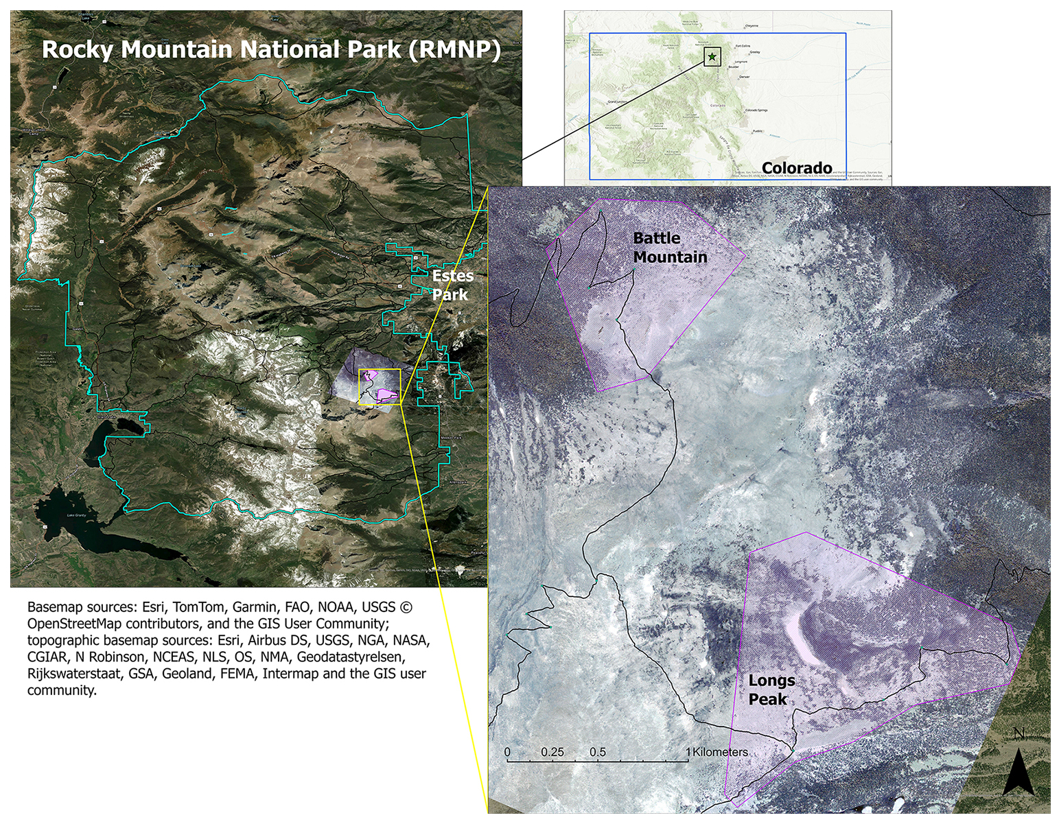
Figure 1 Locations of study areas and WV-3 imagery within RMNP and Colorado. The boundary of Colorado can be seen in blue in the top right inset map. The RMNP boundary is in pale green in the left map; the town of Estes Park is marked for reference. The study areas (Battle Mountain and Longs Peak) are purple polygons visible over the WV-3 imagery extent, displayed in RGB (Red = red band, Green = green band, Blue = blue band) in both the map on the left and the enlarged inset map on the right.

Limber pine is a dominant conifer at treeline in both study areas (Sindewald et al., 2020). The Longs Peak treeline study area communities include dense willow (Salix glauca L., Salix brachycarpa Nutt., and hybrids), Engelmann spruce (Picea engelmannii Engelm.), subalpine fir (Abies lasiocarpa (Hook.) Nutt.), glandular birch (Betula glandulosa Michx.), and quaking aspen (Populus tremuloides Tidestr.). The Battle Mountain treeline study area communities are predominately composed of limber pine with Engelmann spruce, subalpine fir, willow, and glandular birch as minor components.

2.2 Orthorectification and Atmospheric Correction

We collected ground control points (GCPs) at trail junctions and switchbacks, using a Trimble Geo7x Centimeter edition geolocator with a Zephyr 2 antenna mounted on a 1 m carbon fiber pole. GCPs are high-accuracy (5–10 cm) positions of select landscape features visible in satellite imagery. We documented each GCP collection with photos from several angles, indicating the precise location of the point (see Fig. A2), as well as image chips (see Fig. A3) with the position marked from Google Earth Pro (Fig. A3).

Maxar performed rigorous orthorectification to correct for distortions due to terrain; they did this using the nearest neighbor resampling method (preserving the original data values) with the GCP positions and documentation we provided. We requested the nearest neighbor resampling method specifically, to preserve the original reflectance values, as opposed to any method that would substitute the original values with a statistical summary or interpolated value. Cubic convolution resampling is commonly used because it results in a smoother image, but it alters the data values, effectively introducing noise into the data. “Pansharpening” is a similarly inappropriate technique for any analysis that relies on data precision; pansharpening artificially improves the spatial resolution of datasets by modelling statistical relationships between coarser-resolution multispectral imagery with finer-resolution panchromatic imagery and interpolating likely values. The result may aid in visual interpretation for humans, but no new real information is being provided to a CNN. Each larger multispectral pixel is a mixture of spectral signatures of objects at the finer resolution; moving to the finer resolution makes assumptions about the relationship between the two datasets that introduce error and distortions into the data. The coarser-resolution multispectral data may not have enough information for realistic assumptions to be made, and it is likely this approach would inflate the sample size without adding new information. It is possible that more recent deep-learning-based methods of pansharpening could achieve high enough spectral fidelity to justify the step, but we chose to use the data in their native resolutions and adjust our CNN architecture to accommodate the several spatial resolutions. This way, we are still allowing the CNN to learn from the higher-resolution panchromatic data without inflating the sample size of our multispectral data.

Maxar also applied the atmospheric compensation (ACOMP) correction to the imagery, which uses cloud, aerosol, water vapor, ice, and snow (CAVIS) band data collected at the same instance as the multispectral data to identify and correct for atmospheric influences (Pacifici, 2016).

2.3 Field Collections of Polygons Delineating Species Patches

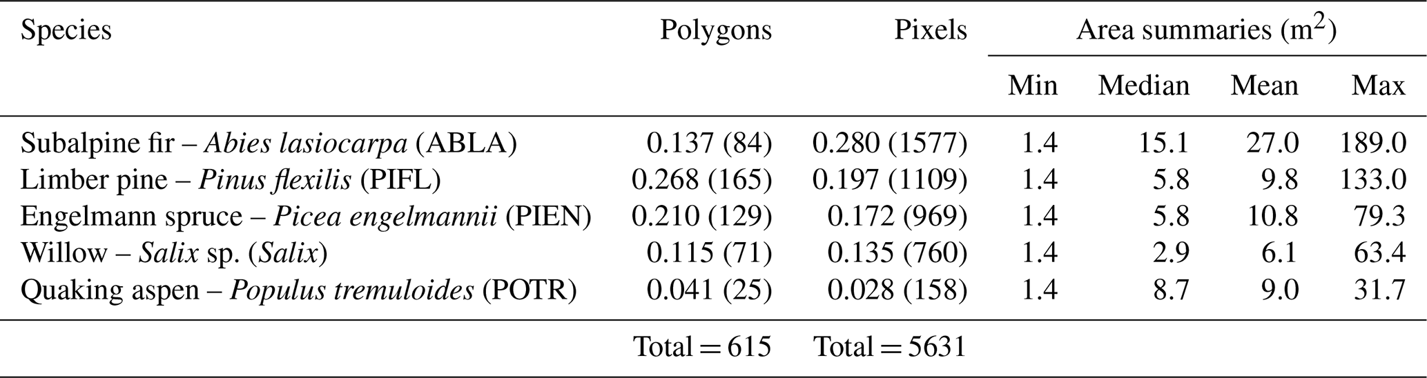
In both study areas combined, we delineated 615 polygons of contiguous, single-species tree/shrub patches in the field that included a total of 165 limber pine, 129 Engelmann spruce, 84 subalpine fir, 71 willow, 141 glandular birch, and 25 aspen (a minor component of the treeline community) (Table 1). The species selected for classification are abundant at these treeline sites and are representative of dominant tree and shrub species at treeline in RMNP. Two shrub species that are also abundant were excluded because they form smaller patches at treeline with areas below the image resolution (less than 1.2 m): common juniper (Juniperus communis L.) and shrubby cinquefoil (Dasiphora fruticosa (L.) Rydb.). A large sample size is necessary to capture the intraspecies variation at treeline in plant condition caused by differences in frost desiccation, wind damage, or water availability, which influences the near-infrared wavelengths in particular (Curran, 1989; Campbell and Wynne, 2011).

We delineated species polygons over five field seasons (2019–2023) to obtain the largest sample size possible in the time available. Our haphazard selection (vs. strict randomization) of species patches that met our criteria was also intended to enable us to obtain as many samples as possible. Species patches were delineated if they were (1) greater than approximately 1 m in area and (2) purely a single species with no contamination from co-occurring species. Ideally, patches were selected which were separated from other tree and shrub species by alpine tundra or rock, but this was not always possible. If patches were bordered by other species or if two pure species patches adjoined, we paused collection to walk to the opposing side of the patch before resuming collection, creating a straight line to indicate greater caution during the later labelling process to ensure training pixels were selected which did not contain any of the adjacent species. We walked the perimeter of each polygon with a Trimble GeoXT or a Geo7x, using differential correction enabled to obtain achieve sub-meter accuracy (typically 10–60 cm at treeline).

Each polygon contained one or more individuals of one given species; apart from limber pine, all of these species may spread clonally at treeline, making discrimination of individual trees or shrubs impossible without a genetic analysis. Limber pine has multi-stemmed growth forms at treeline, but multiple stems may comprise different individuals originating from a single Clark's nutcracker (Nucifraga columbiana (Wilson, A, 1811)) cache of limber pine seeds, presenting the same difficulties (Tomback and Linhart, 1990; Linhart and Tomback, 1985).

We imported the polygon data to ENVI (version 4.8, Exelis Visual Information Solutions, Boulder, CO) and selected multispectral WV-3 pixels that fell entirely within the bounds of each of the polygons. We examined both the panchromatic and multispectral imagery to identify systematic offsets between the polygons and vegetation patches in the imagery. A slight offset of approximately 0.5 m was identified, which reduced the number of viable polygons and pixels for inclusion. We used the shapes of the vegetation patches in the panchromatic imagery and the shapes of the polygons to identify the correct locations of polygons in the imagery and select only pixels that fell within the field-delineated vegetation patches with high confidence. A single operator performed all pixel labelling, and that operator was most often the person in the field delineating patches. The multispectral and panchromatic images were orthorectified together; the pixels aligned across bands and sensors – 4 × 4 panchromatic pixels align precisely with one multispectral pixel. We then exported the reflectance data from each region of interest as CSV files.

Table 1 Class frequencies (proportion of total pixels) for the CNN models. Frequencies are out of 615 polygons and 5631 pixels, respectively. CNNs use a pixel-based classification approach (sample unit = the pixel, not the plant). Table summaries are of labelled region of interest polygons as opposed to the raw, field-delineated polygons; not all field-delineated polygons were useful. The areal summaries are for region of interest polygons.

2.4 Topographic Data

We obtained a 10 m digital elevation model (DEM) from the U.S. Geological Survey EROS Data Center. These raster data are generated by the National Mapping Program from cartographic information and are freely available from the National Map Data Delivery website (https://www.usgs.gov/the-national-map-data-delivery, last access: 25 January 2022). We interpolated the DEM to the resolution of the multispectral data, using a cubic spline resampling method.

2.5 Convolutional Neural Network (CNN) Modelling Methods

We chose to use CNNs to leverage spatial patterns in species distributions. While treeline sites are notoriously heterogeneous, variations in topography and existing vegetation are known to shape snow distribution, which in turn shapes future distribution of plant species due to variation in water availability during the growing season (Hiemstra et al., 2002; Malanson et al., 2007; Zheng et al., 2016). Furthermore, species like Engelmann spruce and subalpine fir tend to co-occur due to similar site preferences and facilitative interactions (Burns and Honkala, 1990; Hessl and Baker, 1997; Gill et al., 2015). All these tendencies translate to spatial patterns detectible in satellite imagery, and CNNs are built to detect patterns in gridded data.

In this section, we describe the methods we used to train the CNN models. Section 2.5.1. introduces CNNs for unfamiliar readers. Section 2.5.2 contains an overview of the CNN model architecture, including an adaptation to allow training on the higher resolution panchromatic imagery before concatenating those data with the multispectral imagery and DEM. Section 2.5.3 provides an overview of the hyperparameter experiment, used to determine the optimal combinations of fixed hyperparameters for the best model performance. In ML models, parameters are the trainable weights and biases within the models, and hyperparameters are values the user pre-defines that guide the training process and do not change during training. Section 2.5.4 describes the explainable artificial intelligence (XAI) methods used to determine which predictors were most important for model performance.

While we describe the CNN architecture first (in Sect. 2.5.2) to explain how the CNN works and is built, the specific architecture was determined in part by the results of several hyperparameter experiments (Fig. 2). The first two hyperparameter experiments are described in Sect. S1.3 and S1.4 of the Supplement, and the final hyperparameter experiment is described in detail in Sect. 2.5.3.

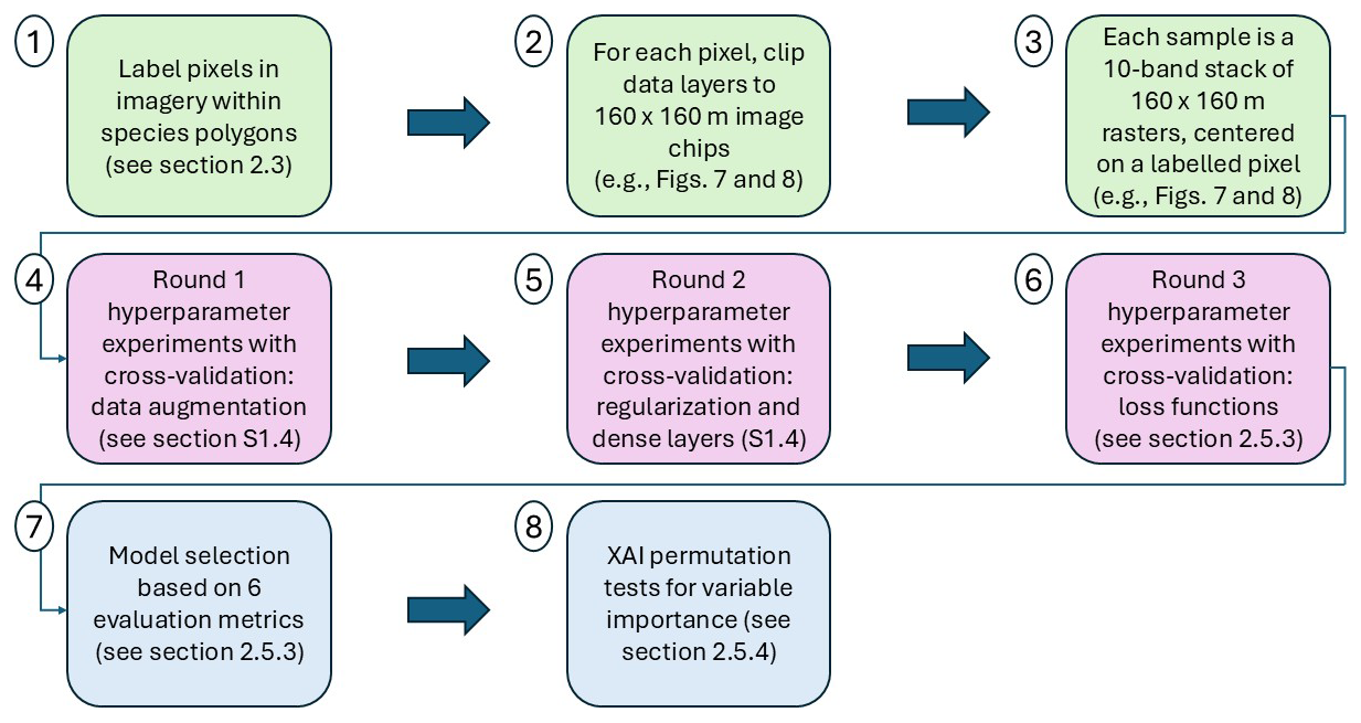
Figure 2 Workflow overview diagram. The first three steps (green) outline how the image data were prepared as image chips prior to CNN model development (see Sect. 2.3 and example inputs in Figs. 7 and 8). In steps four and five, we trained models with varying levels of data augmentation and regularization (see Sect. S1.3 and S1.4 of the Supplement). We used five-fold cross-validation for every variation of each hyperparameter experiment. In steps five and six we experimented with different numbers of dense layers (see Sects. S1.4 and 2.5.3) and in step six we also experimented with six different loss functions. Following the hyperparameter experiments (purple), we proceeded with selecting the best-performing models based on six evaluation metrics (see Sect. 2.5.3). We then ran permutation tests with the top-performing models – an explainable artificial intelligence (XAI) method – to assess variable importance (see Sect. 2.5.4).

2.5.1 Introduction to CNNs

CNNs are a form of neural network that can be spatially aware, detecting patterns in gridded data on multiple spatial scales, and are often used for image recognition tasks (Goodfellow et al., 2016d; Dubey and Jain, 2019). A CNN is structured as a series of convolutional blocks, each containing one or more convolutional layers and ending with a pooling layer (Dubey and Jain, 2019). Each convolutional layer contains many convolutional filters, or “kernels”, containing learned parameters (weights and biases). During convolution, the input channels (or data layers, e.g., the multispectral WV-3 data contain eight channels) are multiplied by a 3-D convolutional filter, typically with dimensions of 3 pixels × 3 pixels × number of input channels. The products of this multiplication are summed to create one pixel in the output feature map (Goodfellow et al., 2016a). The filter slides over the spatial grid of the input imagery; at each position in this grid, it generates one pixel of the output feature map. To produce the desired number of feature maps (M), a convolutional layer contains M filters. Classic image-processing also uses convolutional filters, but the weights are pre-determined. For example, there are known, 3 × 3-pixel kernels that achieve blurring, sharpening, edge detection, etc. A strength of CNNs is that these weights are learned rather than pre-determined. The CNN uses multiple different filters to learn different patterns in the data (detecting edges, textures, parts of objects, whole objects, etc.), which generate multiple feature maps that are sent to the next convolutional layer. (The number of feature maps generated is a fixed hyperparameter set by the user). The resulting feature maps (matrices containing the results of the convolutions) can be thought of as patterns found across all data channels. CNNs may be thought of as “a feature-detector (the convolution and pooling layers) attached to a traditional neural network”, which learns from these detected features and transforms them into predictions (Lagerquist, 2020).

Parameters in a CNN consist of weights and biases in the convolutional filters. A single convolutional filter contains one bias and $K_{\mathrm{h}}\cdot K_{\mathrm{w}}\cdot C_{\mathrm{in}}$ weights, where K_h is the height of the filter in pixels; K_w is the width in pixels; and C_in is the number of input channels. Thus, a single convolutional layer contains C_out biases and $K_{\mathrm{h}}\cdot K_{\mathrm{w}}\cdot C_{\mathrm{in}}\cdot C_{\mathrm{out}}$ weights, where C_out is the number of filters or output feature maps. The model is trained in a series of epochs; in each epoch, the CNN learns from a series of many batches of training samples. In the first epoch, all the weights and biases start from a random initial seed. The first batch of data is input to the CNN, and the loss function is calculated. The loss function is an error metric used to “tell” the ML model how right or wrong it is in its predictions – a feedback mechanism. After the model learns from the training samples in an epoch, the weights and biases are adjusted through backpropagation (explained in detail in Sect. S1.1), using rules of gradient descent to minimize the loss function (the measure of model error).

Another batch of data is fed to the CNN, the loss function is calculated, and backpropagation is repeated. This process repeats for B training batches each containing N data samples, where B and N (both positive integers) are hyperparameters. At the end of the epoch, the validation loss is computed, using data in the validation fold. This in turn repeats for P epochs or stops early once the loss function for the validation fold (also known as out-of-bag error) has not decreased in the last Q epochs, where P and Q (both positive integers) are hyperparameters. The process of training a machine learning (ML) model with small batches (minibatches) of randomly selected training data is known as stochastic gradient descent, and is the most common algorithm used for training by contemporary ML developers to create deep learning models (Goodfellow et al., 2016c, b; Li et al., 2014).

Most of the methods we use are standard in the ML literature, but we recognize our audience may include treeline ecologists for whom these methods are new. We provided further explanations of CNN methods – and their importance – for interested readers in Supplement Sect. S1, including loss functions (Sect. S1.1 and Appendix B), backpropagation (Sect. S1.1), ReLU activation (Sect. S1.2), batch normalization (Sect. S1.2), data augmentation (Sect. S1.3), and dropout (S1.3).

2.5.2 CNN Model Architecture

We trained all CNN models using Keras (version 3.10.0) application programming interface for TensorFlow (version 2.19.0) in Python (version 3.11.5). We used all eight multispectral WV-3 bands, the panchromatic band, and the interpolated DEM as the CNN inputs, yielding a total of 10 channels. A CNN model is a pixel-based classification approach, with a variable number of pixels within each tree or shrub polygon. Before modelling, the data were subset into 160 × 160 m image chips, each centered on one training pixel – one point within one tree or shrub polygon. This initial sub-setting process streamlined the dataset, reducing the RAM and time required to run the model.

The pixel dimensions of each image chip varied by the spatial resolution of the data: 513 × 513 pixels for the panchromatic imagery (31 cm resolution), and 129 × 129 pixels for the multispectral imagery and the interpolated DEM (1.24 m resolution). We adapted the model architecture to accommodate this discrepancy, to leverage the information in the higher-resolution panchromatic imagery, while ensuring that all 10 data channels could be processed together within the CNN. The first two convolutional blocks in the CNN processed only panchromatic imagery (at 31 cm resolution). Each convolutional block consisted of two convolutional layers (with a 3-by-3 convolutional filter), followed by 2-by-2 pooling, which reduces the spatial resolution by half. Hence, in two convolutional blocks, the 513 × 513 panchromatic data were downsampled via max pooling to 257 × 257 (62 cm resolution) and then to 129 × 129 (1.24 m resolution), matching the resolution of the multispectral and interpolated DEM data (Fig. 3). Max pooling helps with edge detection and allows the model to learn patterns on larger spatial scales. Using our classification problem as an example, the CNN could first learn size and shape patterns for species morphologies, associated with the spectral data, and, after pooling, could learn that certain species are found near other species or landscape features at coarser scales (such as rivers, or places of low or high prominence in the DEM). For a more detailed description of each convolutional block, please see Appendix C.

Figure 3 CNN architecture for the six-class model, incorporating panchromatic, multispectral, and DEM inputs at different spatial resolutions. Each convolutional block is represented by a green box labeled “Conv” (actually two series of convolution and activation, followed by batch normalization) and an orange half-oval labeled “Max-pool”. After two convolutional blocks with only the panchromatic data, the multispectral and interpolated DEM data were concatenated with the feature maps from the convolutional blocks (“Concat”). At the end, the feature maps (64 of them, each with 5 × 5 pixels) were flattened (all of the values in all of the feature maps are appended to a 1-D vector, 3200 values long) and followed by one classic NN dense layer (or “fully connected layer”), yielding a vector of six probabilities, one for each class. At each step, the dimensions of the image patch are indicated in pixels, as well as the number of feature maps. For example, the first Conv step yielded four feature maps of 513 × 513 pixels.

After two convolutional blocks, once the panchromatic data were pooled down to the resolution of the multispectral imagery and the interpolated DEM, those channels were concatenated (“Concat” in Fig. 3). Seventeen channels (one raw DEM channel, eight raw multispectral channels, and eight feature maps based on the one panchromatic channel) were fed into the next convolutional block. Then, after five more convolutional blocks (each halving the spatial resolution while increasing the number of feature maps), the last feature maps were flattened (re-organized into a 1-D vector) and fed into a dense layer, or “fully connected layer”. A traditional (spatially agnostic) NN contains only dense layers, which are vectors of values connected to every adjacent value, including all the values in the next (and previous) dense layer(s).

Following the dense layer, we used the softmax activation function to force outputs to range from 0–1 with a sum of 1 (interpretable as probabilities representing all possible events/classes in the sample space) (Goodfellow et al., 2016d). The non-terminal dense layers included a dropout rate of 0.650, and every convolutional and dense layer used an L₂ regularization strength of 10^−6.5. Dropout and L₂ regularization are both regularization methods that help prevent the CNN from overfitting to the training data (see Sect. S1.3 for details). These were fixed hyperparameters, determined to be the best settings via the hyperparameter experiment described in Sect. 2.5.2.

The total number of training samples was 5631. We validated the models using five-fold cross-validation, so for each model, we used four-fifths of our data for training and the remaining fifth of the data for validation. We split the training and validation by individual – for a given organism, either (1) all of the pixels for that organism were in the training set or (2) all of the pixels were in the validation set. After creating the folds, we performed data augmentation (Goodfellow et al., 2016a), turning each original training sample into eight augmented samples. To do this, we first normalized the data, transforming the data from physical values (x) to z-scores (z) based on the mean and standard deviation of each training fold. Data should be separated into training and validation folds before normalization, because otherwise we would be leaking information about the full data distribution from the validation data into the training data. To create an augmented data sample, we add Gaussian noise to the predictors in the original sample, with a mean of 0.0 and standard deviation of 0.2. (The parameters of the Gaussian distribution from which we drew the noise were fixed hyperparameters.) Thus, the final sample size for the training dataset was 45 048 image chips (5631 × 8 augmented samples).

During each epoch, the model was trained with all 45 048 data samples in batches of 64 samples each (703 total batches). Each model was trained for 100 epochs, with a command to stop training early if the loss function did not improve for 15 epochs. We trained all CNN models with the Adam optimizer, using all the Keras defaults, including an initial learning rate of 0.001. The Adam optimizer updates the learning rate after every epoch and adjusts learning rates separately for every model parameter (every weight or bias) (Goodfellow et al., 2016b; Kingma and Ba, 2014). We determined the optimal loss function for our classification problem through the hyperparameter experiments (described in the next Sect. 2.5.2.).

We trained three CNN models, each with a different number of classes. Classification becomes more difficult with each additional class. We pooled classes with fewer data to see whether that would improve model performance, particularly for distinguishing limber pine from the other species with higher accuracy. In addition to the six-class model, we trained a four-class model to separate the three conifers (limber pine, Engelmann spruce, and subalpine fir) from each other and from the deciduous plants (glandular birch, willow, and aspen), the latter grouped together in one class as “Other”. Lastly, because managers may find it useful to discriminate limber pine from other treeline species, we trained a two-class model with limber pine and the other species grouped as “Other”. The CNN architecture for the four- and two-class models was the same as the six-class model, except for the output layer. The output layer produces one probability per class, so its output vector varied in length from two to six (Figs. C1 and C2).

2.5.3 Hyperparameter Experiments and Model Selection

We ran hyperparameter experiments separately for the six-,
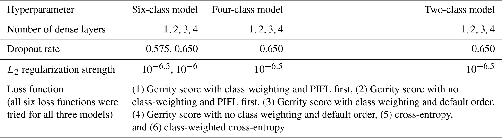
four-, and two-class models (see Supplement Sect. S1.5 for detailed information on what each hyperparameter does within a CNN). Hyperparameters have a strong influence on model performance, so it was important to test a subset of hyperparameter combinations to identify the best versions of the six-, four-, and two-class models. The same four experimental hyperparameters were used for all three experiments: the number of dense layers at the end of the model, the dropout rate (used for non-terminal dense layers, i.e., all dense layers except the output layer that provides the final probabilistic predictions), the L₂ regularization strength (used for all convolutional and dense layers), and the loss function. Table 2 summarizes the values tested for each hyperparameter for each of the three models. The candidate values tested in the experiment for each hyperparameter were chosen for their usefulness in training skillful CNN models in past work (Lagerquist et al., 2019, 2020, 2021). We also tested a wider range of values for (1) the number of dense layers, (2) dropout rate, and L₂ weight (see Supplement Sect. S1.4).

As part of the hyperparameter experiment, we trained the models with two loss functions: cross entropy and the Gerrity score. Cross-entropy is widely used for classification problems; it comes from the field of information theory and describes the bits required to distinguish two distributions (i.e., the distribution of predictions from the distribution of observations) (Lagerquist, 2020). The class frequencies in our dataset were quite unbalanced (Table 1), so we also tested the Gerrity score, which rewards “risky” predictions. That is, in a problem with unbalanced classes, the Gerrity score rewards correct predictions of a lower-frequency class (which are harder) more strongly than correct predictions of a higher-frequency class (which are easier) (Gerrity, 1992). Equations for these metrics can be found in Appendix B and in other published works (Lagerquist et al., 2019; Lagerquist, 2020).

The Gerrity score depends on how classes are ordered numerically. For example, in a six-class problem, the Gerrity score rewards correct predictions of “class 1” more strongly than correct predictions of “class 6”, even if both classes have equal frequency. Thus, by default, we ordered classes from least to most frequent (using the pixel-based class frequencies in Table 1). We also tested the Gerrity score with two modifications. One was the class-weighted Gerrity score, where each data sample in the loss function was weighted by $\ln \frac{\mathrm{1}}{f}$ or ln 50, whichever was lower, where f is the frequency of the correct class. Class-weighting makes the Gerrity score reward risky predictions even more. The second modification was the limber-pine-first (PIFL-first) Gerrity score, where the aforementioned list was reordered to make limber pine “class 1”. The PIFL-first Gerrity score gives higher rewards for correct predictions of limber pine. The Gerrity score varies between −1 and 1. A higher score is better, and as long as it is above 0, the model is performing better than a random model (Lagerquist et al., 2019).

Table 2 Experimental hyperparameter values tested for the six-, four-, and two-class models.

In the six-class experiment, the total number of hyperparameter combinations was 96, representing all possible combinations of four numbers of dense layers, two dropout rates, two L₂ regularization strengths, and six loss functions (Table 2). For every hyperparameter combination (hyperparameter model) we performed five-fold cross-validation, thus training five sub-models; we refer to each set of five cross-validated sub-models as one model (Fig. 4). This yielded a total of 480 sub-models for the six-class experiment (96 × 5) and 120 sub-models for each of the smaller experiments (24 × 5). To evaluate the performance of each hyperparameter model, we used predictions only on out-of-bag samples. For each model, every data sample was out-of-bag, appearing in the validation fold rather than one of the training folds only once. Given that our dataset contained 5631 samples, the results for each hyperparameter model were therefore based on 5631 out-of-bag predictions.

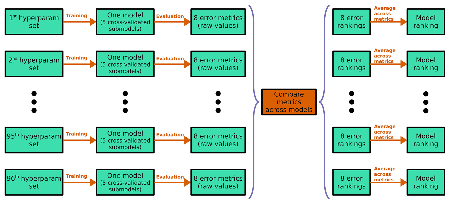
Figure 4 Schematic for the six-class hyperparameter experiment. The two- and four-class experiments follow the same methodology, except with 24 hyperparameter sets (hence, 24 models) instead of 96. Each row corresponds to one model; the black ellipsis (dots) represent the 3rd through 95th models; each green box represents an object (hyperparameter set, model, set of error metrics or rankings); and each orange arrow/box represents a procedure. The purple braces indicate that models are being compared with each other – i.e., they indicate a procedure that cannot be done independently for each model. The last procedure – implied but not shown – is choosing the model with the best “Model ranking”, averaged over all eight error metrics.

We considered eight evaluation metrics: (1) top-1 accuracy, (2) top-2 accuracy, (3) top-3 accuracy, (4) cross-entropy, (5) Heidke score, (6) Peirce score, (7) Gerrity score, and (8) PIFL-first Gerrity score. Top-k accuracy is the fraction of data samples for which the correct class is in the k highest probabilities output by the model; for example, top-2 accuracy is the fraction of data samples for which the correct class is one of the two classes predicted with the highest probability. Top-1 accuracy is usually just called “accuracy”, i.e., the fraction of samples for which the correct class receives the highest probability from the model. Further discussion of all metrics, including mathematical and conceptual definitions, can be found in Appendix B. We ranked each model in terms of each evaluation metric out of the total number of models attempted in the experiment. For the six-class experiment, these rankings were out of 96; for the smaller experiments, these rankings were out of 24. Then, for each model, we averaged its rankings over all eight metrics. The model with the best average ranking was chosen as the best model.

2.5.4 Permutation Tests

Permutation tests are a form of XAI (McGovern et al., 2019), methods that enable interpretation of ML model results in terms of the predictors used. The permutation test comes in four varieties: the single-pass forward, multi-pass forward, single-pass backward, and multi-pass backward. The permutation tests successively permute (shuffle) or de-permute (clean) the values of predictor variables and quantifying the impact that has on model performance. For data with correlated predictors, each variety of the test gives different results (McGovern et al., 2019). Our image data contain both spatial autocorrelation, where nearby pixels are correlated with each other, and spectral correlation, where nearby wavelength bands in the multispectral imagery are correlated with each other. These problems always arise in image data, meaning that methods assuming mutual independence cannot be used. It is important to examine all four varieties of the test and determine which results are consistent to draw robust conclusions.

In the permutation test, permuting a predictor variable refers to shuffling the values of that variable across all data samples (in our case, across all out-of-bag samples), breaking the relationship between the predictor and the target variable (in our case, the species class). In the single-pass forward test, only one predictor variable is permuted at a time, leaving the other variables unchanged. After permuting one predictor variable, the model performance on the clean dataset is compared to performance on the dataset with that variable permuted. If model performance drops significantly with the predictor permuted, then that predictor is considered very important. In the multi-pass forward test, the single-pass forward test is carried out iteratively. Step 1 begins with a clean dataset and determines the most important variable, x_1st, which is then permuted for the duration of the test. Step 2 begins with the output from step 1 (a dataset with x_1st permuted and all other variables unchanged) and determines the second-most important variable, x_2nd, which is then permuted for the remainder of the test. This continues until all predictor variables are permuted. In the single-pass backward test, we begin with a completely randomized dataset, where all predictor variables are permuted. Then only one predictor variable is cleaned up (restored to the correct order) at a time, leaving the other variables permuted. After cleaning up one predictor variable, we measure how much this improves model performance compared to the completely randomized dataset. If the model performance improves significantly when the predictor is cleaned up, then that predictor is considered very important. In the multi-pass backward test, the single-pass backward test is carried out iteratively. Step 1 begins with a completely randomized dataset and determines the most important variable, x_1st, which is then cleaned up for the duration of the test. Step 2 begins with the output from step 1 (a dataset with $x_{\mathrm{1}\mathrm{st}}^{*}$ cleaned up and all other variables still permuted) and determines the second-most important variable, x_2nd, which is then cleaned up for the remainder of the test. This continues until all the predictor variables have been cleaned.

3 Results

3.1 Hyperparameter Experiment Results

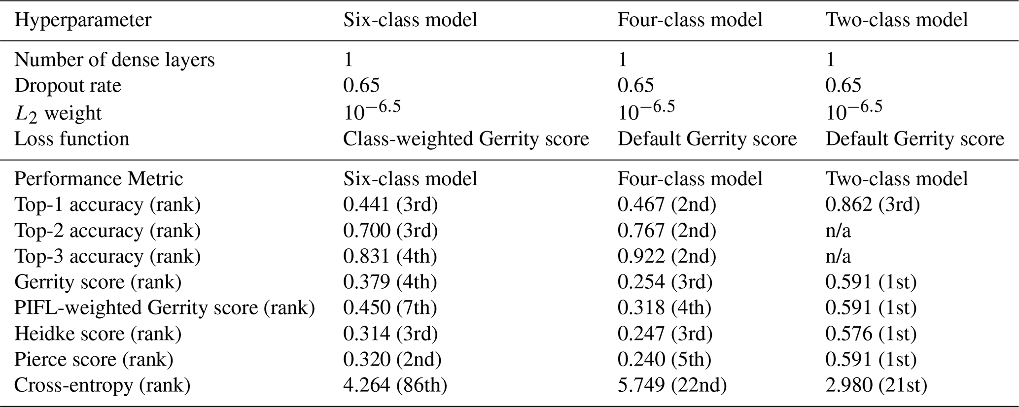
The hyperparameters for each of the selected models (six-class, four-class, and two-class) are shown in Table 3. Figure 5 shows the top-1 accuracy for all models in the six-class experiment. The selected model (circle) had accuracies of 0.44, 0.70, and 0.83 (top-1, top-2, and top-3, respectively), whereas the model with the highest top-1 accuracy (star) had accuracies of 0.45, 0.67, and 0.81. The selected model performed much better on the Gerrity score (0.38 vs. 0.30), comparably on the Heidke and Peirce scores (0.31 and 0.32 vs. 0.32 and 0.32), and only marginally worse on the PIFL-first Gerrity score (0.45 vs. 0.49). The selected model was the best model out of 96 models based on the average of all eight metrics.

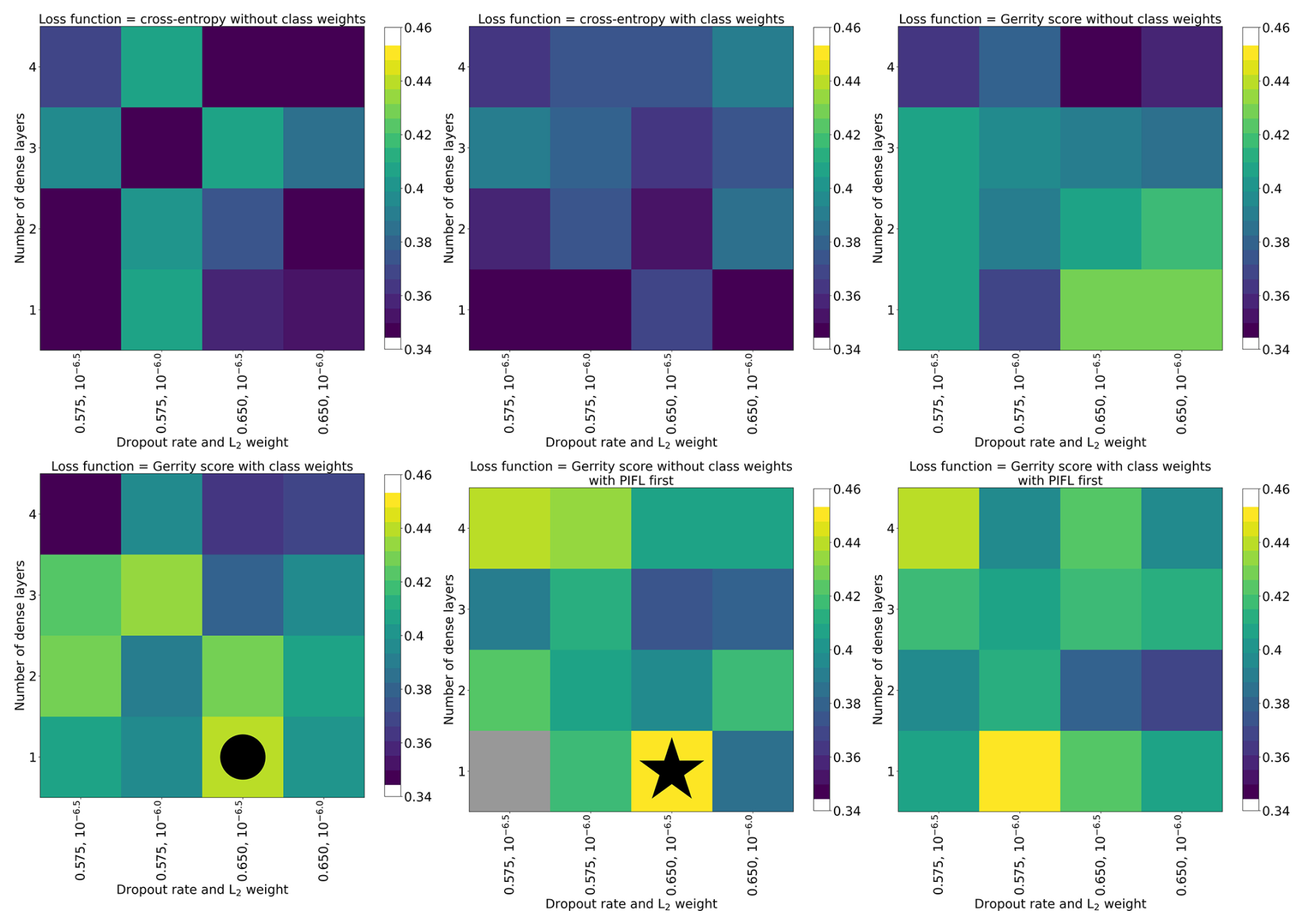
Figure 5 Hyperparameter experiment results for the six-class classification, evaluated by top-1 accuracy. Each grid cell of the figure shows results from a single CNN model (one set of hyperparameters), including results from all five sub-models. In the case of every data sample, the prediction came from a CNN that was not trained on that data sample. The color indicates the top-1 accuracy of the model. The models are organized by their hyperparameter values. The circle indicates the model that was selected from the set. The star indicates the model with the highest top-1 accuracy.

The selected four-class model was the best out of 24 evaluated, with the second-highest ranking for each top-k accuracy, as well as high rankings for the remaining metrics (Table 3). The selected two-class model was again the best balance out of 24 evaluated; it was the top-performing model based on the Gerrity, PIFL-weighted Gerrity, Heidke, and Peirce scores, and was the 3rd best model based on top-1 accuracy (Table 3). Strangely, across the board, models that performed well based on the cross-entropy metric performed poorly based on the other 7 metrics. See Supplement Sect. S2 for the remaining hyperparameter experiment result figures (Figs. S1–S21).

Table 3 Hyperparameters and model performance metrics for the top-performing models. The rank of the selected model with respect to each performance metric is indicated in parentheses. Ranks are out of 96 for the six-class model and out of 24 for the four- and two-class models. All metrics are positively oriented (higher is better) except for cross-entropy, which is negatively oriented. n/a: not applicable.

3.2 Six-Class Model Results

The six-class model performance was good considering the complexity of the task and the spatial and spectral resolution of the data, with a top-1 (overall) accuracy of 44.1 % and a top-2 accuracy of 70.0 % (Table 3). By comparison, a trivial model would have a top-1 accuracy of 28.0 % and a top-2 accuracy of 47.6 %. For a trivial model, the predicted probability of class k is always the frequency of class k in the data. In other words, a trivial model's predictions are the same for every data sample. For the six-class problem, a trivial model would always predict 28.0 % probability of subalpine fir, 18.9 % probability of glandular bitch, etc. (Table 1).

Using the class-weighted Gerrity score was effective, leading to higher overall model performance and for the correct identification of minority classes, though the model performed best at distinguishing the two highest-frequency classes: subalpine fir and limber pine (Fig. 6). Figure 6 shows the classes which the model correctly identified with the greatest frequency, as well as the species it most often tended to confuse.

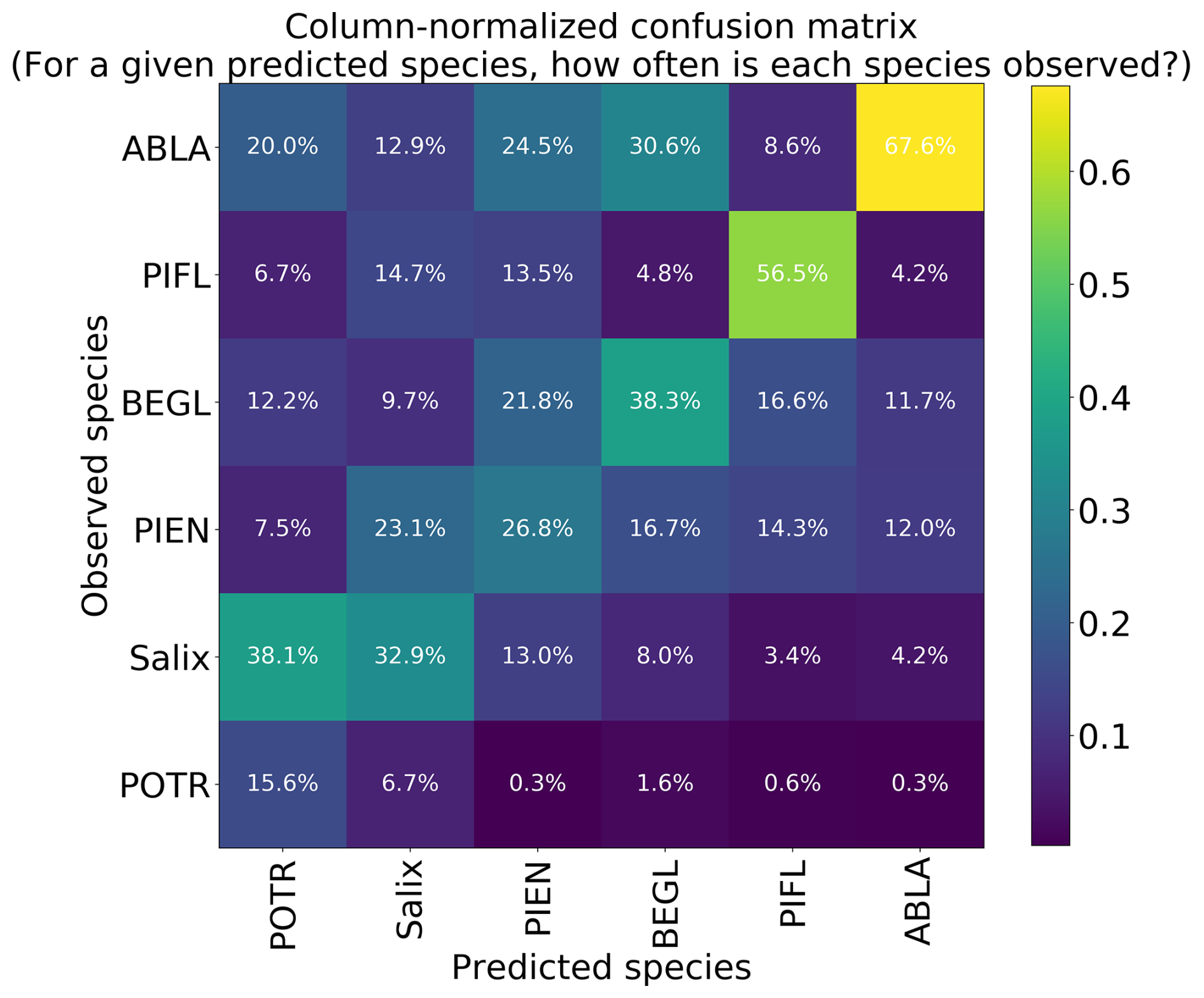
Figure 6 Column-normalized confusion matrix for the six-class model. Classes include subalpine fir (ABLA), glandular birch (BEGL), Engelmann spruce (PIEN), limber pine (PIFL), aspen (POTR), and willow (Salix).

Limber pine was most often confused with willow and Engelmann spruce in the six-class model (Fig. 6), likely because of the model's reliance on the panchromatic band (see Figs. 8b, d, and S39). While limber pine does not grow as true krummholz at treeline (Holtmeier, 2009), it is stunted and flagged and resembles willow or other shrubs in the panchromatic imagery. Figure 7 shows an example of a “best hit” identification of limber pine from the six-class model, which correctly predicted limber pine with 100 % probability. The example is representative of the dispersed pattern and small size of limber pine at treeline. See Supplement Sect. S5.1 for other best hits.

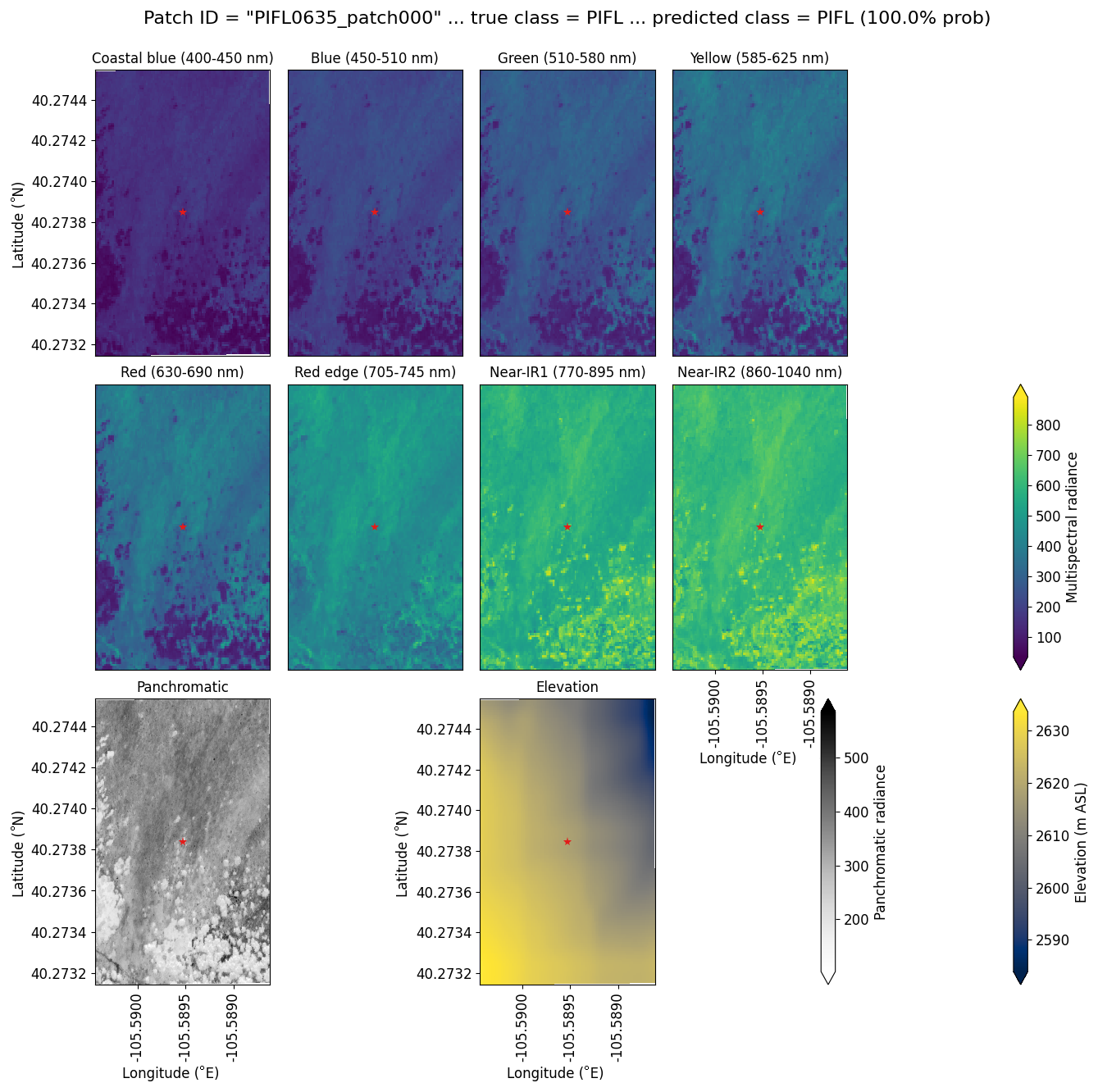
Figure 7 An example of a “best hit” classification of PIFL from the six-class model, where the model correctly predicted PIFL with 100 % probability. This example (image chip or patch) is from the Battle Mountain study site. All eight multispectral bands, the panchromatic band, and the DEM are shown. The red star in the center of each image patch is the pixel being classified. Units of radiance are W m⁻² sr⁻¹ µm⁻¹.

Subalpine fir was most often confused with glandular birch, once again likely due to reliance on textural information in the panchromatic band (Figs. 9b, d, and S43 in Supplement Sect. S4); both species form large patches on the landscape that appear similar without additional structural information, such as height. Engelmann spruce was the least distinguishable after aspen, which was a lower-frequency class and has a similar growth pattern (in the panchromatic imagery) to both glandular birch and subalpine fir. Engelman spruce and subalpine fir tend to co-occur (with the same elevational distribution) (Sindewald et al., 2020; see also Figs. S44, and S45). Their mean spectral radiance curves appear to be statistically distinguishable in the coastal blue, blue, green, yellow, red, and red edge bands (Fig. S27), but the CNN relied less on these bands (Fig. 8). An example of a worst-case confusion between Engelmann spruce and subalpine fir can be seen in Fig. 8. Although the panchromatic band was very important for model performance (Fig. 9b and d), likely due to its high spatial resolution, it was not enough to distinguish the treeline forms of these species by their morphology or spatial distribution on the landscape.

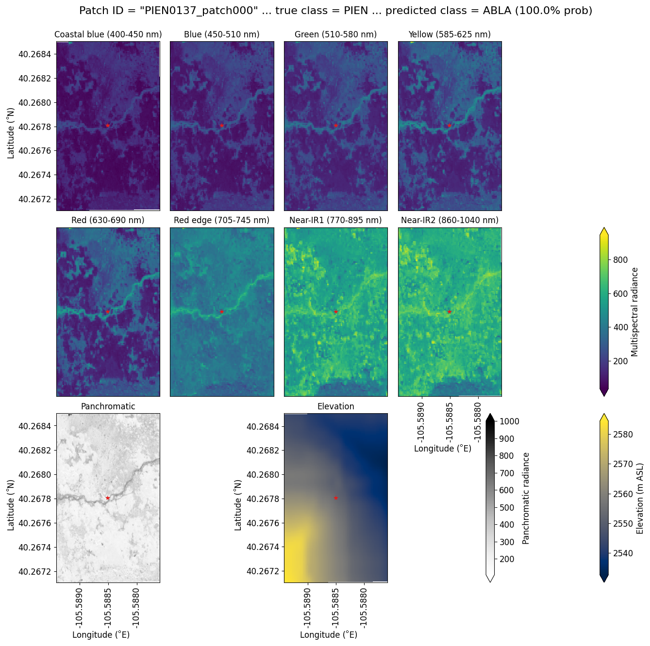
Figure 8 An example of a “worst confusion” classification of PIEN as ABLA from the six-class model, where the model incorrectly predicted PIEN as ABLA with 100 % probability. This example (image chip or patch) is from the Longs Peak study site. All eight multispectral bands, the panchromatic band, and the DEM are shown.

Based on the results of the permutation tests, elevation was the most important predictor for model performance (Fig. 9a, b, and d), which makes sense biologically. Willow species thrive in riparian areas, and at the Longs Peak site they are typically found along creeks or in topographic depressions where snow gathers (Fig. S47). Similarly, glandular birch, subalpine fir, and Engelmann spruce grow more abundantly in areas where late-lying snowpack provides moisture through the start of the growing season (Figs. S43 and S44) (Burns and Honkala, 1990; Hessl and Baker, 1997; Gill et al., 2015). Limber pine, by contrast, is a drought- and stress-tolerant conifer that often occupies on convex sites or wind-swept ridges where snow is blown clear (McCune, 1988; Ulrich et al., 2023; Steele, 1990). The spatial distribution of species samples and the spatial accuracy of model predictions can be seen in Appendix D. In figure D1a, we see that willow, in particular, clusters near a riparian area of the Longs Peak study area. However, the models did not exclusively predict species where they are most often found. While the models appear to be relying on elevation to make use of spatial patterns in species distributions, the models are not exclusively relying on topographic data (Figs. D1 and D2).

Several multispectral WV-3 bands were also important for model performance, as evidenced by the multi-pass forward and backward tests (Fig. 9b and d), including red, green, yellow, coastal, blue, and near-IR2. The visible bands emerged as important predictors for distinguishing aspen from the other species in the six-class model (Fig. S46). While the multispectral bands were clearly important, they did have as strong an influence on model performance as did elevation or the panchromatic band, indicating the six-class CNN model did not rely on those data as heavily (Fig. 9).

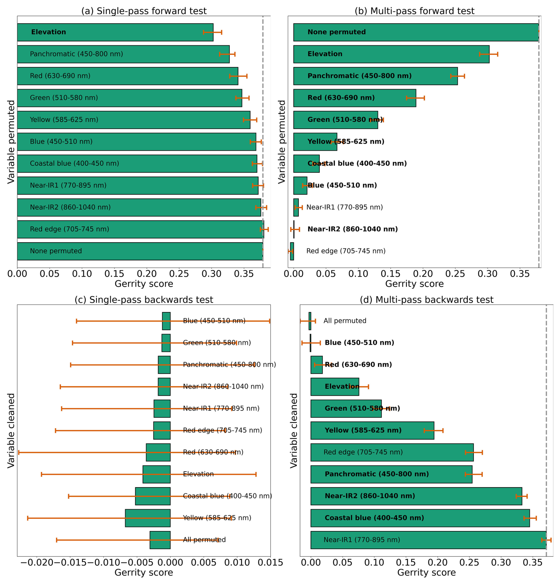
Figure 9 Results from each kind of permutation test to assess predictor importance for the six-class model. Predictors in bold have a significant effect on model performance when permuted, according to a 95 % confidence interval over 100 random perturbations of the given predictor. Within each panel, predictor importance decreases from top to bottom, so the most important predictors are at the top. Our evaluation metric for this permutation test is the Gerrity score.

3.3 Four-Class Model Results

The four-class model performed slightly better than the six-class model overall, with top-1 and top-2 accuracies of 46.7 % and 76.7 %, respectively (Table 3). A trivial model could at most have top-1 and top-2 accuracies of 35.1 % and 63.1 %, respectively. The model was best at correctly identifying subalpine fir, with the predicted species being correct 60.4 % of the time (Fig. 10). The model did least well at correctly identifying limber pine (39.3 %), confusing it with the deciduous species pooled into the “Other” class. Engelmann spruce was the lowest frequency class in the four-class dataset (17.2 % of the samples), and since the top model was trained with the default Gerrity loss and not the PIFL-first Gerrity loss, the model was most penalized for incorrect classification of Engelmann spruce. The result was that the four-class model was almost twice as effective at identifying Engelmann spruce as the six-class model (50 % vs. 26.8 %).

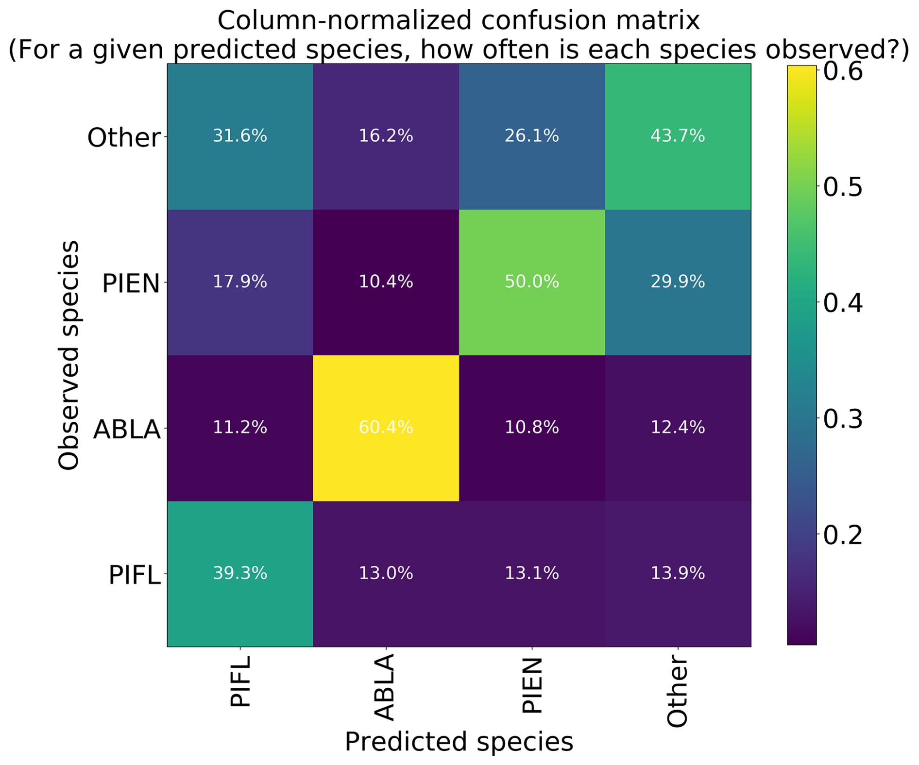
Figure 10 Column-normalized confusion matrix for the four-class model. Classes include subalpine fir (ABLA), Engelmann spruce (PIEN), limber pine (PIFL), and other classes pooled as “Other”.

The permutation tests were consistent in showing the importance of the panchromatic data to four-class model performance (Fig. 11a, b, and d). As discussed above, the high spatial resolution of the panchromatic data likely allowed the CNN to distinguish growth forms and patterns of species occurrence and co-occurrence on the landscape (Figs. D3 and D4). The panchromatic band emerged as the most important predictor for all four classes (Figs. S48–S51). Multispectral bands red, green, blue, and yellow also emerged as significant predictors (Fig. 11b and d), particularly for correct identification of ABLA, PIEN, and Other (Figs. S48, S49, and S50).

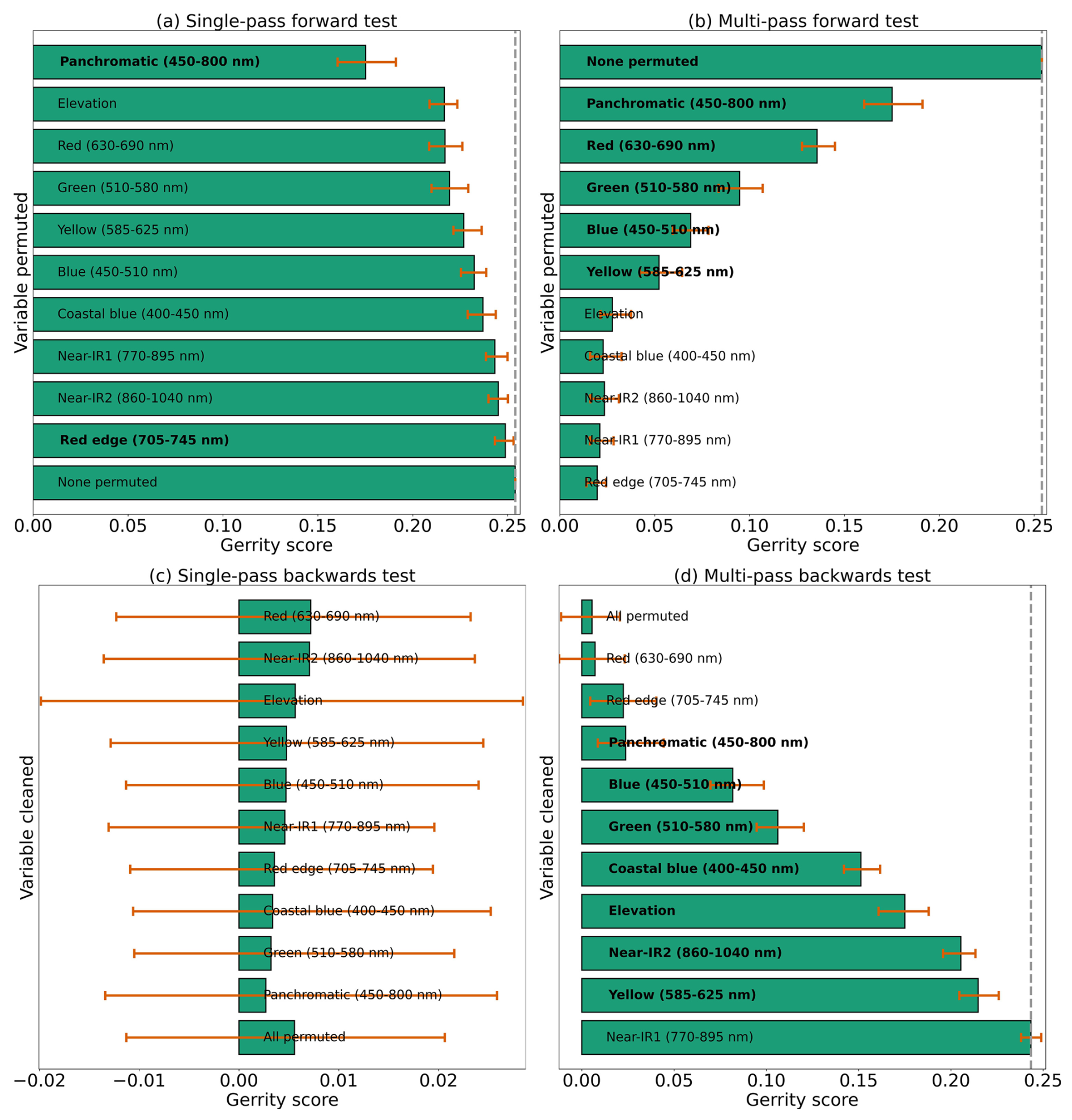
Figure 11 Results from each variety of the permutation test to assess predictor importance for the four-class model. Formatting is explained in the caption of Fig. 10.

3.4 Two-Class Model Results

The two-class model had the highest top-1 accuracy at 86.2 %, though much of this skill is attributable to its correct prediction of the majority class (“Other”); a trivial model would have a top-1 accuracy of 80.3 %, which is the frequency of Other. The model correctly identified limber pine 64.0 % of the time (Fig. 12), which is still an improvement over the success rates for the six-class (56.5 %) and four-class (39.3 %) models.

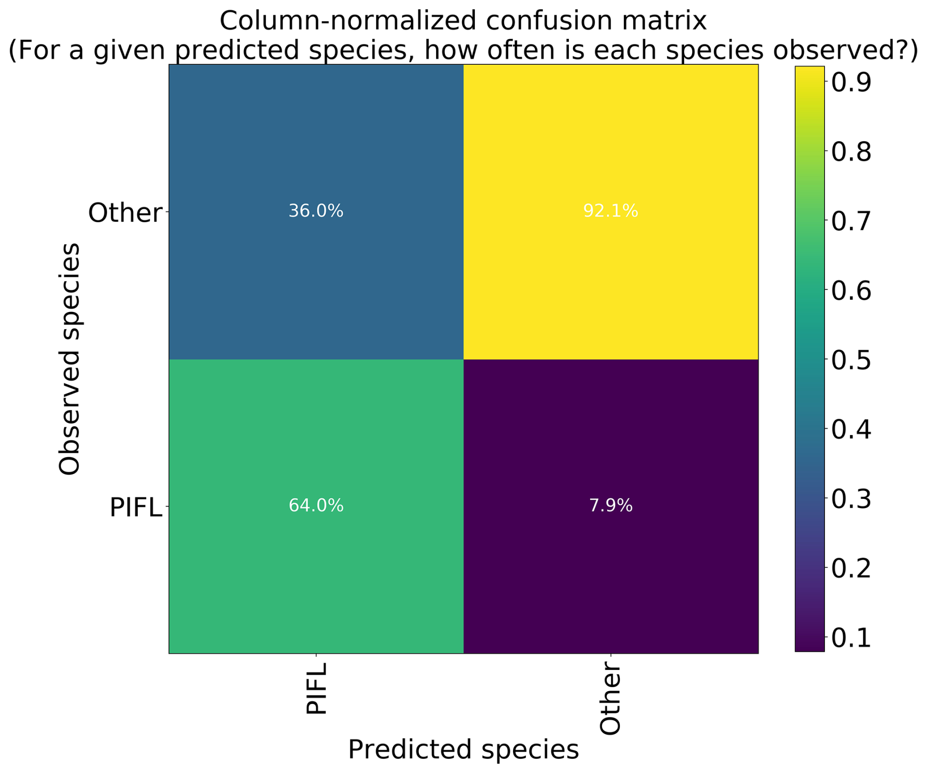
Figure 12 Column-normalized confusion matrix for the two-class model. Classes include limber pine (PIFL) and other classes pooled as “Other”.

With the goal of distinguishing limber pine from other treeline species, the panchromatic band emerged as the most important predictor by far – nearly half the model skill depended on the higher spatial resolution panchromatic band (Fig. 13a, b, and d). The red, yellow, green, and blue bands were also important for discriminating limber pine from other species. Limber pine tends to form low-density stands, with individuals spaced almost evenly across the landscape (Figs. 6, D5, and D6). Unlike subalpine fir and Engelmann spruce, limber pine also does not form large, sprawling krummholz mats or grow in large patches like glandular birch, willow, and aspen. The relatively lower spatial resolution of the multispectral WV-3 bands may have limited the usefulness of these data for distinguishing limber pine, although several bands were still significant predictors in the permutation tests for limber pine (Fig. S52).

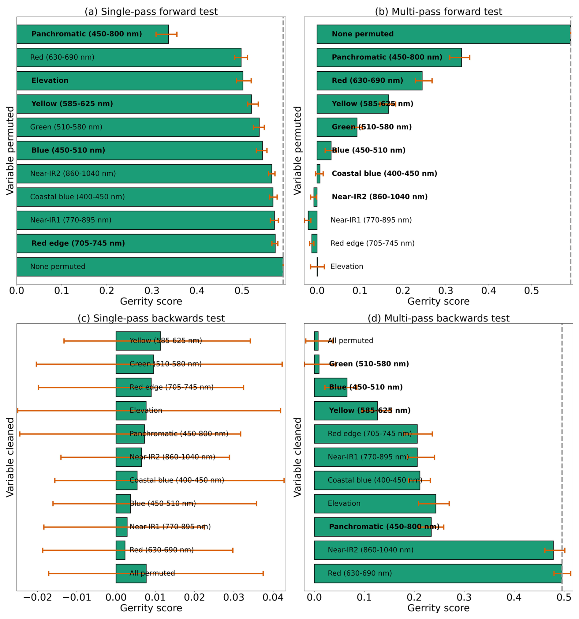
Figure 13 Results from each variety of the permutation test to assess predictor importance for the two-class model. Predictors in bold have a significant effect on model performance when permuted, according to a 95 % confidence interval over 100 random perturbations of the given predictor. Within each panel, predictor importance decreases from top to bottom, so the most important predictors are at the top. Our evaluation metric for this permutation test is the Gerrity score.

4 Discussion

This study may be the first attempt to use satellite imagery to identify woody plant species in a treeline ecosystem. Our goal was to discriminate six alpine treeline tree and shrub species in the Southern Rocky Mountains, using a pixel-based Convolutional Neural Network (CNN) classification of high-resolution Worldview-3 (WV-3) satellite imagery. We were particularly interested in identifying limber pine from other treeline species, especially since it is a species of conservation concern and its distribution at treeline in Rocky Mountain National Park is incompletely known.

4.1 Overview of CNN Model Performance

Overall, our results had mixed success. The six-class model performed reasonably well given the difficulty of the problem, with 44.1 % top-1 and 70 % top-2 accuracy – much better than a trivial model could achieve (28.0 % and 47.6 %, respectively). The four-class model did not improve classification accuracy as much as expected, with 46.7 % top-1 and 76.7 % top-2 accuracy (vs. 35.1 % and 63.1 %, respectively, for a trivial model). The simplified two-class model achieved a fairly high overall accuracy of 86.2 % (vs. 80.3 % for a trivial model). The two-class model distinguished limber pine from other trees and shrubs with 64.0 % accuracy, which, on its own, may not be useful for more than identifying regions of treeline where high-probability limber pine pixels tend to cluster. However, the model did notably well (92.1 %) at identifying pixels that are not limber pine.

4.2 Predictor Importance

The panchromatic band was the most important predictor based on the results of the XAI permutation tests, both for overall model performance in all three models, and for identifying limber pine specifically. This makes sense both biologically and in terms of the model structure. The models were trained on the panchromatic imagery for two convolutional blocks before the multispectral and elevation data were introduced to the model; this architectural design allowed us to make use of the higher resolution panchromatic data to detect fine-scale spatial patterns, and it likely also reinforced the mathematical influence of these data in the final model predictions. Treeline species often have distinctive physiological growth responses to stressors (e.g., high winds and heavy snowpack), and their krummholz growth forms vary in their spatial patterns. Limber pine frequently occurs as a solitary tree on the landscape, occupying very few pixels and surrounded by alpine tundra (Sindewald et al., 2020). Other species are more likely to form larger patches through vegetative layering and are also more likely to co-occur on the landscape. The CNN models still relied heavily on the panchromatic data for these species, but they also made greater use of the multispectral imagery for discrimination among these species.

Elevation was the second most important predictor for six-class model performance after the panchromatic band. When discerning among six species classes, the CNN clearly picked up on topographic patterns in species distribution on the landscape. The species of willow classified here (Salix glauca L., Salix brachycarpa Nutt., and hybrids) are most abundant near creeks in the Longs Peak study area, with aspen not much farther away (Cooper, 1908). This may generalize when the model is applied at a broader geographic scale; willow and aspen tend to be found in regions with more moisture (Baker, 1989; Coladonato, 1993; Uchytil, 1992; Howard, 1996). Engelmann spruce and subalpine fir tend to be found further from creeks, but in topographic depressions with late-lying snowpack (Burns and Honkala, 1990; Hessl and Baker, 1997; Gill et al., 2015). Glandular birch and limber pine are more often found on slopes, and limber pine occupies windswept ridges with early snowmelt (McCune, 1988; Ulrich et al., 2023; Steele, 1990; Cooper, 1908).

Multispectral bands were consistently identified as important predictors, suggesting that the CNN model utilized the multispectral imagery despite its lower spatial resolution, compared with the panchromatic imagery. The visible bands detect variation in concentrations of photosynthetic pigments in the leaves, which differ among species. The near-infrared (N-IR) region of the spectrum varies based on cellular structure, which changes with water content, making N-IR bands useful for assessing plant health (e.g., the normalized difference vegetation index or NDVI) (Curran, 1989; Campbell and Wynne, 2011). Trees vary widely in condition at treeline due to varying levels of frost desiccation, wind damage, or water availability (Tranquillini, 1976, 1979). The relatively lower importance of the N-IR bands for discriminating species at treeline may mean that damage to trees and shrubs introduces variation across species that almost overshadows species-specific responses to these stressors.

However, the lower importance of the N-IR and red edge bands may also be because the CNN models prioritized the higher resolution spatial data and spatial patterns of species distributions in the panchromatic imagery over their spectral differences. Table S1 of Sect. S3 of the Supplement summarizes the WV-3 bands where pairs of species may be statistically distinguished. Each pair of species differs in at least one band except for Engelmann spruce and willow, which overlapped across all eight bands. Interestingly, species pairs commonly differed significantly in the near-infrared bands. The fact that these bands were less important for CNN performance suggests that the models relied on panchromatic data first and only used the multispectral or DEM data second – whenever the panchromatic data were not informative. In those cases (e.g., cases where species growth forms were similar), the models made greater use of the DEM and visible bands. It is possible that the near-infrared bands are more correlated with the panchromatic band, and so the models obtained little additional information from the N-IR and red edge bands. This is plausible given that both the near-infrared bands and the panchromatic band are responsive to plant structure.

4.3 Model Generalizability

While our models have been validated through five-fold cross-validation, we need to test these models on the classification of geographically distinct treeline communities. Machine learning models tend to over-fit models, which is why we employed several regularization methods to reduce the risk of overfitting and to improve generalizability (see Supplement Sect. S1.4). However, the importance of the elevation data in species classifications, despite its low original resolution of 10 m, suggests that these models could have learned idiosyncratic topographic patterns at the two study sites (i.e., the “Clever Hans” problem, where machine learning models pick up on signals in the data that are sometimes collinear with more meaningful signals, much like the popular history horse, Clever Hans, who could respond to emotional anticipation in humans but could not, in fact, count) (Lapuschkin et al., 2019; Pfungst, 1911). If the models learned that moisture-sensitive species tend to occur in topographic depressions, where snow persists into the spring, they could still generalize well to other treeline locations. The figures showing spatial model performance (Appendix D) were encouraging in this respect; we saw no obvious spatial biases indicating that the models only performed well for different species when they were located in hotspots of species occurrence at a given site. On the other hand, if the models relied on proximity to a creek that ran through the study site, they may perform less well at treeline sites at comparable elevations but without a creek. In future work, we will test these models on a geographically independent dataset.

4.4 Trade-offs of Computation and Data Acquisition Costs and Increases in Model Accuracy

The use of combined hyperspectral and lidar data is increasingly considered the gold standard for identifying trees with remote sensing data, but our work opens the door for more cost-effective methods for researchers and managers. Ørka and Hauglin (2016) compared remote sensing data acquisition costs and found that high-resolution commercial satellite imagery is much less expensive than airborne aerial imagery (Ørka and Hauglin, 2016). Cost estimates do not include subsequent computational costs incurred through the analysis of such datasets, which can also represent a barrier for wider-scale implementation; not every manager and researcher has the training or money to make use of supercomputing resources.

WV-3 potentially represents a better balance of cost and classification accuracy. WV-3 imagery is cheaper than aerial imagery and provides comparable resolution. The addition of ACOMP atmospheric correction is important, because this method uses CAVIS data collected simultaneously with the multispectral and panchromatic data, yielding highly accurate corrections (Pacifici, 2016). However, as our study showed, even WV-3 data may have spatial resolution that is too low for classification of treeline vegetation species.

UAS data may yield better results than WV-3 given their very high spatial resolution (sub-meter). In fact, Onishi and Ise (2021) demonstrated that a classification accuracy of over 90 % for seven species can be achieved using only red-green-blue (RGB) imagery, classified with a CNN (Onishi and Ise, 2021). These authors also used an XAI method, guided Grad-CAM, to determine that the CNN was focusing on canopy shapes for its classification. Our findings support theirs: spatial resolution is important for tree species classification problems. The UAS approach may also be best for classification problems requiring high temporal resolution (e.g., monthly). If data collection spans multiple years or multiple seasons, the UAS approach may be the most cost-effective. UAS, however, are prohibited on some public lands in the United States, particularly in national parks and congressionally designated wilderness areas, which include most treeline areas of conservation interest.

5 Conclusions

To our knowledge, we are the first to use satellite imagery to distinguish tree and shrub species in alpine treeline ecosystems (Garbarino et al., 2023). Our study approach fills an important methodological gap, enabling researchers to connect landscape- and local-level treeline patterns and local treeline processes by leveraging field research on treeline species. Species-level maps of alpine treeline would enable researchers to better stratify field sampling efforts to understand interspecies dynamics, as well as how species tolerances influence treeline elevation advance (or lack thereof).

Our models have proven useful for identifying probability hotspots for limber pine occurrence at treeline, supporting ongoing research and management of this ecologically important conifer. Our methods are also more cost-effective than techniques relying on hyperspectral and lidar data collected with aircraft and are applicable to a broader geographic extent than UAS. Our work may also support the ongoing research and conservation of limber pine in the Rocky Mountains of the U.S. and Canada (Schoettle et al., 2019).

However, we believe that adapting these models to an object-based classification approach will improve classification accuracies and allow landscape-level species identification without the need to train additional models. We anticipate that outputs from our CNN models, in the form of pixel-level probability maps for classified species, may be easily processed into segmented images of tree and shrub objects for object-based classification. While beyond the scope of the present work, segmentation and object-based classification will be the necessary next steps to apply these methods at a landscape scale. Once these methods are developed, we may be able to use satellite imagery to map limber pine's distribution at treeline and monitor the distribution of this important species as climate changes.

Appendix A: Field Methods

Collecting ground control points (GCPs) with a multispectral satellite without tasking the satellite (and placing targets) is quite challenging; we selected GCPs opportunistically, aiming to cover as much of the image as possible. Much of the image, especially lower in elevation, was forested, and taller trees obscured ground features. Much of the rest of the image was tundra, with very few targetable features. We collected GCPs at the corners of switchbacks and at trail junctions, always at or above treeline where these features could be clearly seen in the image. We were able to collect 15 GCPs (Fig. A1), six of which were in the Battle Mountain study area and four of which were in the Longs Peak study area.

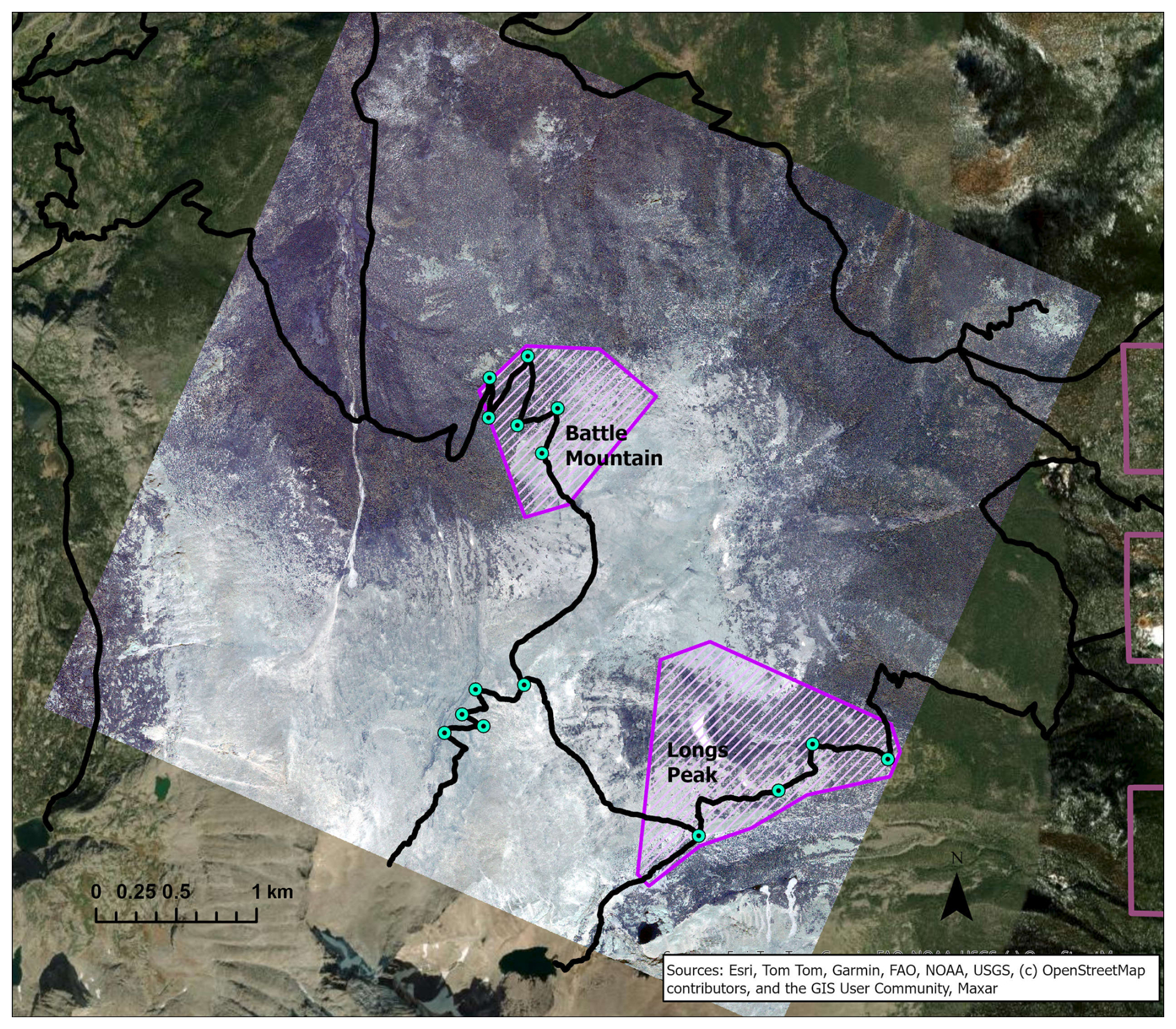
Figure A1 Teal points mark the locations of ground control points collected in Rocky Mountain National Park over the WV-3 satellite image, displayed in RGB. The Battle Mountain and Longs Peak study areas are delineated in purple. Trails are marked with black lines. Please see Fig. 1 for copyright details.

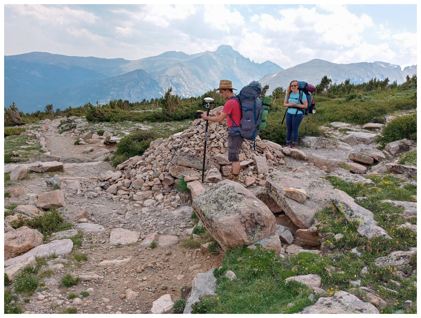
Figure A2 Lucas Rudasill and Laurel Sindewald collecting a ground control point and descriptive metadata at the corner of a switchback next to a cairn in RMNP. This photo was included, with the GPS data, descriptive metadata, and image chips, to inform MAXAR orthorectification.

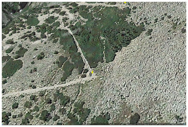
Figure A3 Example of an image chip from Google Earth Pro with the GCP position marked precisely on the image, corresponding to the photo documentation in Fig. 26. This image chip was included, with the GPS data, descriptive metadata, and photos, to inform MAXAR orthorectification. © Google Earth.

Appendix B: Loss Functions and Model Evaluation Metrics

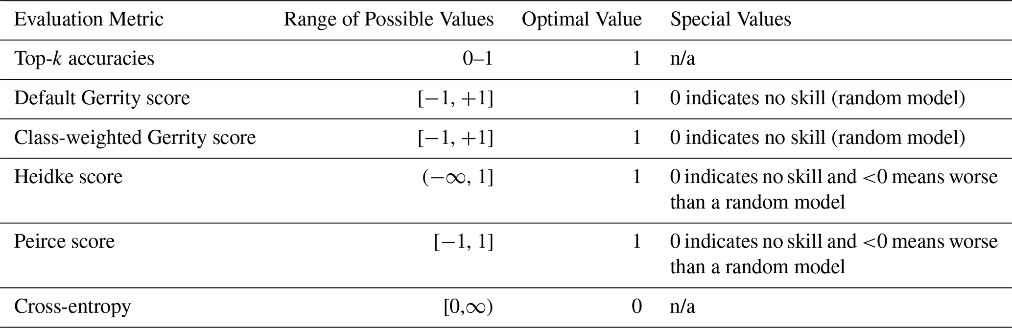
We used eight metrics for model evaluation: top-1, top-2, and top-3 accuracies, the Gerrity score, the PIFL-first Gerrity score, the Heidke and Peirce scores, and cross-entropy. Note that evaluation metrics, used to assess the performance of an already-trained model, are not necessarily the same as the loss function used for training. Only the Gerrity score, PIFL-first Gerrity score, and cross-entropy were used as loss functions in this study. Table B1 summarizes characteristics of each metric.

Table B1 Characteristics of metrics used for model evaluation. n/a: not applicable.

Equation (B1) shows how the Gerrity score is calculated, without additional class-weighting (Gerrity, 1992).

$$\begin{array}{}\text{(B1)}& \left\{\begin{array}{l}\text{Default GS}=\frac{\mathrm{1}}{N}\sum _{i=\mathrm{1}}^K\sum _{j=\mathrm{1}}^K{\text{n}}_{ij}{s}_{ij},\\ s_{ij}=s_{ji}=\frac{\mathrm{1}}{K-\mathrm{1}}\left[\sum _{k=\mathrm{1}}^{i-\mathrm{1}}{a}_k^{-\mathrm{1}}-\left(j-i\right)+\sum _{k=j}^{K-\mathrm{1}}{a}_k\right],\\ a_k=\frac{\mathrm{1}-\frac{\mathrm{1}}{N}{\sum }_{r=\mathrm{1}}^{k}n\left(y_r\right)}{\frac{\mathrm{1}}{N}{\sum }_{r=\mathrm{1}}^{k}n\left(y_r\right)}\end{array}\right.\end{array}$$

where N is the total number of data samples, K is the number of classes, i and j index the predictions and observations, respectively, and n_ij is the number of data samples with the ith class predicted and jth class observed. When i=j (when the prediction matches the observation), s is positive and higher to reward the correct prediction. When i≠j, s is lower or even negative to penalize the incorrect prediction. s_ij is in turn determined by the second function in Equation B1, which determines the weights based on class frequencies to increase the reward when a low-frequency class is correctly predicted and decrease the penalty when a low-frequency class prediction is incorrect. In the second function, which determines the s_ij weights, a_k is the cumulative observation frequency of the first k classes and is defined in the third function. n(y_r) is the number of data samples where the rth class is correct.

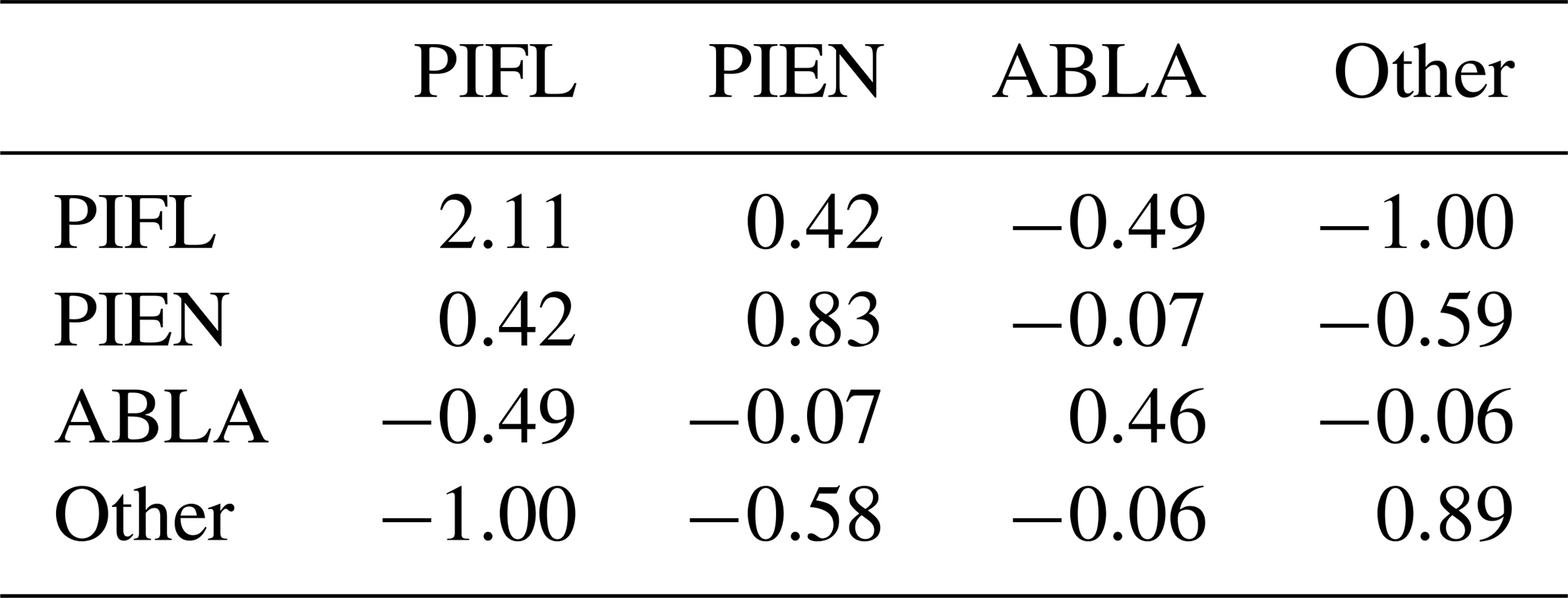
Table B1 is an example of an s-matrix (a matrix of s_ij weights) for the four-class model. The s_ij weights are larger for classes that have lower frequencies but also depend strongly on the order of the classes. For example, PIEN had a low class frequency (0.172) relative to Other (0.351), so the s_ij (PIEN, PIEN) weight was higher than any of the weights for Other. Because PIEN was the first class indexed for the Gerrity score, and because s_ij is calculated based on a_k, which is the cumulative observation frequency of the first k classes, the (PIEN, PIEN) weight was greater than the (PIFL, PIFL) weight, even though PIFL had the almost same class frequency as PIEN.

Table B2 The s-matrix for the default Gerrity score for the four-class model. The class frequences were 0.172 for PIEN, 0.197 for PIFL, 0.280 for ABLA, and 0.351 for Other.

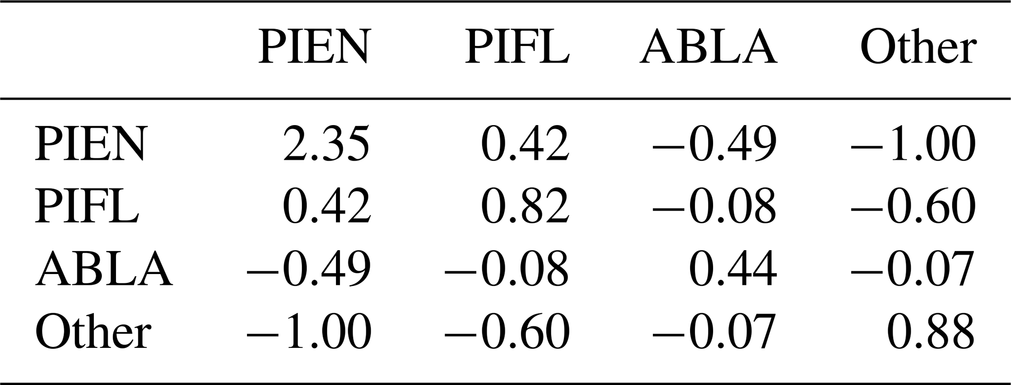
The reverse was true when PIFL was indexed first in the Gerrity score: PIFL had by far the highest weight, even though PIFL had only a slightly lower class frequency than PIEN (Table B3).

Table B3 The s-matrix for the PIFL-first Gerrity score for the four-class model. The class frequences were 0.172 for PIEN, 0.197 for PIFL, 0.280 for ABLA, and 0.351 for Other.

Equation (B1) shows the default Gerrity score, which does not have additional class-weighting. We also added weights to the equation to prioritize the low-frequency classes even more heavily. Equation (B2) shows the class-weighted Gerrity score, which replaces the first function defined in Eq. (B1). (The other two functions remain the same.)

$$\begin{array}{}\text{(B2)}& \text{Weighted GS}=\left\{\begin{array}{l}\frac{{\sum }_{i=\mathrm{1}}^K{\sum }_{j=\mathrm{1}}^K{w}_j{n}_{ij}{s}_{ij}}{{\sum }_{i=\mathrm{1}}^K{\sum }_{j=\mathrm{1}}^K{w}_j{n}_{ij}}\\ w_j=\ln \left(\min \left(\frac{\mathrm{1}}{f_j},\mathrm{50}\right)\right)\end{array}\right.\end{array}$$

where f_jis the observed frequency of the jth class and w_j is the resulting weight. The weighting function we devised limits the degree to which a class can be prioritized by capping the weight at the natural log of 50.

Cross-entropy is simpler than the Gerrity score. Cross-entropy quantifies the number of bits required to distinguish the distribution of model predictions from the distribution of observations. Cross-entropy is calculated using Eq. (B3), and its characteristics are listed in Table B1.

$$\begin{array}{}\text{(B3)}& \mathit{\epsilon }=-{\displaystyle \frac{\mathrm{1}}{N}}\sum _{i=\mathrm{1}}^N\sum _{k=\mathrm{1}}^K{y}_{ik}{\log }_{\mathrm{2}}\left(p_{ik}\right)\end{array}$$

where N is the number of data samples, K is the number of classes, p_ik is the model-predicted probability that the ith sample belongs to the kth class, and y_ik is a binary indication of the correct class, which is 1 if the ith example belongs to the kth class and 0 otherwise.

The Heidke (Heidke, 1926) and Peirce (Peirce, 1884) scores are similar in that they both measure the proportion of correct predictions above and beyond those that would be expected from a random model (Lagerquist et al., 2019). Their equations differ slightly. The Heidke score can be calculated with Eq. (B4) and its domain is listed in Table B1.

$$\begin{array}{}\text{(B4)}& \text{Heidke score}={\displaystyle \frac{\frac{\mathrm{1}}{N}\sum _{k=\mathrm{1}}^K{n}_{kk}-\frac{\mathrm{1}}{N^{\mathrm{2}}}{\sum }_{k=\mathrm{1}}^{K}n\left(P_k\right)n\left(y_k\right)}{\mathrm{1}-\frac{\mathrm{1}}{N^{\mathrm{2}}}{\sum }_{k-\mathrm{1}}^{K}n\left(P_k\right)n\left(y_k\right)}}\end{array}$$

where N is the total number of data samples, K is the total number of classes,n_kkis a correct prediction of class k, n(P_k) is the number of samples where the kth class is predicted, and n(y_k) is the number of samples where the kth class is observed. The Peirce score can be calculated with Eq. (B5) and shares these term definitions.

$$\begin{array}{}\text{(B5)}& \text{Peirce score}={\displaystyle \frac{\frac{\mathrm{1}}{N}{\sum }_{k=\mathrm{1}}^K{n}_{kk}-\frac{\mathrm{1}}{N^{\mathrm{2}}}{\sum }_{k=\mathrm{1}}^{K}n\left(P_k\right)n\left(y_k\right)}{\mathrm{1}-\frac{\mathrm{1}}{N^{\mathrm{2}}}{\sum }_{k=\mathrm{1}}^{K}n{\left(y_k\right)}^{\mathrm{2}}}}\end{array}$$

Appendix C: Convolutional Neural Network Architecture Diagrams (Four- and Two-Class Models)

The panchromatic data were input to the first convolutional block, labeled “Conv 513 × 513 × 4” and “Max pool 257 × 257 × 4” in Fig. 3. All convolutional blocks in our CNN contained two convolutional layers, using 3 × 3-pixel convolutional filters or “kernels”. The first convolutional layer in this block transformed the panchromatic data to two feature maps, via two learned convolutional filters. The second convolutional layer in the block then transformed the two feature maps to four feature maps, via four learned filters. Each convolutional layer was followed by an activation function, which is a pixel-by-pixel non-linear transformation. Activation functions are the key component enabling neural networks to learn non-linear relationships. Our specific activation function was the leaky rectified linear unit (ReLU) with a slope parameter of 0.2 (Nair and Hinton, 2010). Furthermore, each activation function was followed by batch normalization (Ioffe and Szegedy, 2015), which restores values in the maps to an approximately standard normal distribution. (The predictor variables followed a standard normal distribution, ensured by our z-score transform, but the operations carried out in a CNN can warp this distribution, which leads to slower training convergence.) After two convolutional layers with activation and batch normalization, we used max pooling to reduce the spatial resolution by half. With max pooling, the maximum value for each set of four pixels is retained. The full series of convolution > activation > batch normalization > convolution > activation > batch normalization > pooling made up one convolutional block (Figs. 3, C1, and C2). CNN model architecture diagrams for the four-class and two-class models are shown in Figs. C1 and C2, respectively.

Figure C1 CNN architecture for the four-class model, incorporating panchromatic, multispectral, and DEM inputs at different spatial resolutions. The architecture is the same as the six- and two-class models, but with a different number of probabilities output by the final dense layer.

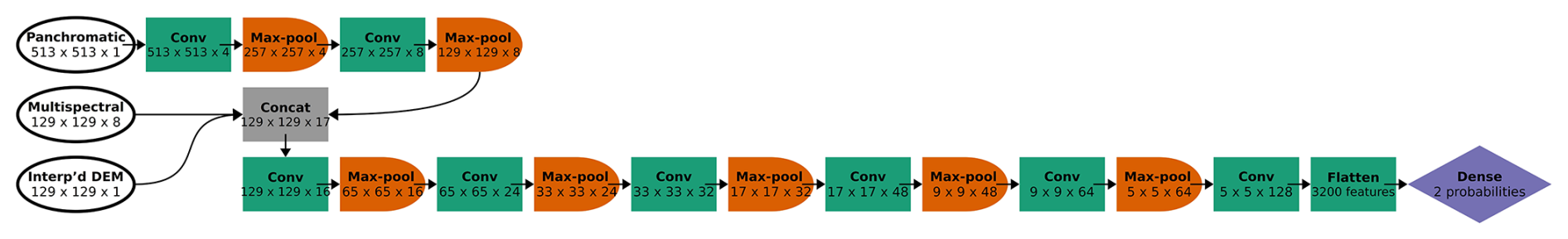
Figure C2 CNN architecture for the two-class model, incorporating panchromatic, multispectral, and DEM inputs at different spatial resolutions. The architecture is the same as the six- and four-class models, but with a different number of probabilities output by the final dense layer.

Appendix D: Spatial Diagrams of Model Performance

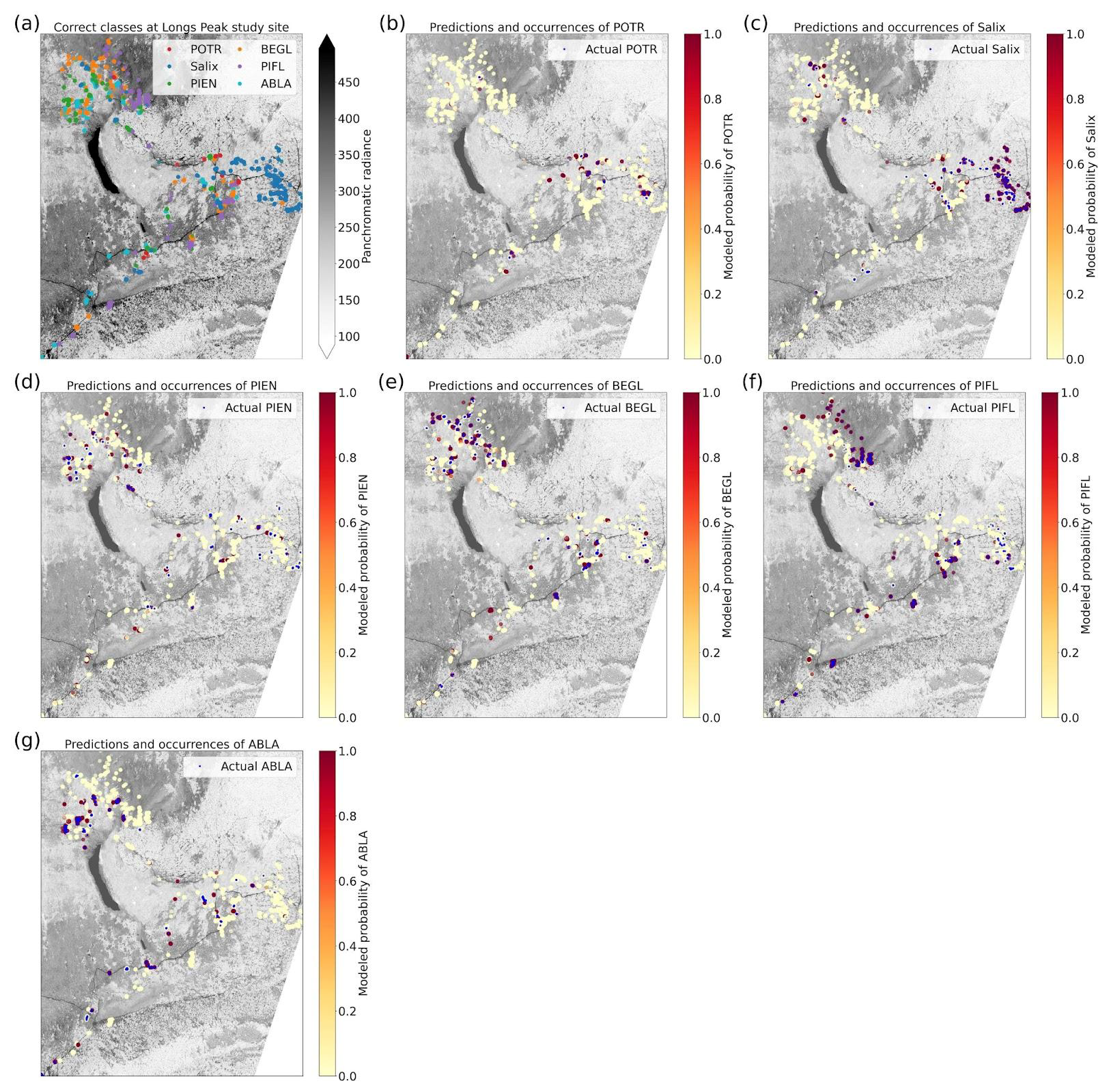
Figure D1 argets and out-of-bag predictions for the 6-class model at the Longs Peak study site. (a) Targets (actual classes) with panchromatic radiance (W m⁻² sr⁻¹ µm⁻¹) plotted in the background.  Panchromatic radiance is plotted at quarter resolution (1.24 m instead of 0.31 m), due to memory limitations. (b) Out-of-bag predictions and actual occurrences of POTR.  For each data sample (one data sample = one polygon pixel, as in Table 1), the yellow-to-red marker shows the modeled probability that the data sample is POTR, while the presence of a blue marker indicates that the sample is actually POTR.  Hence, faint yellow markers (probability ≅0) with no blue marker on top can be considered true negatives; faint yellow markers with a blue marker can be considered false negatives; dark red markers (probability ≅1) with a blue marker can be considered true positives; and dark red markers with no blue markers can be considered false positives. (c) Same as panel b but for Salix. (d) Same but for PIEN. (e) Same but for BEGL. (f) Same but for PIFL. (g) Same but for ABLA.

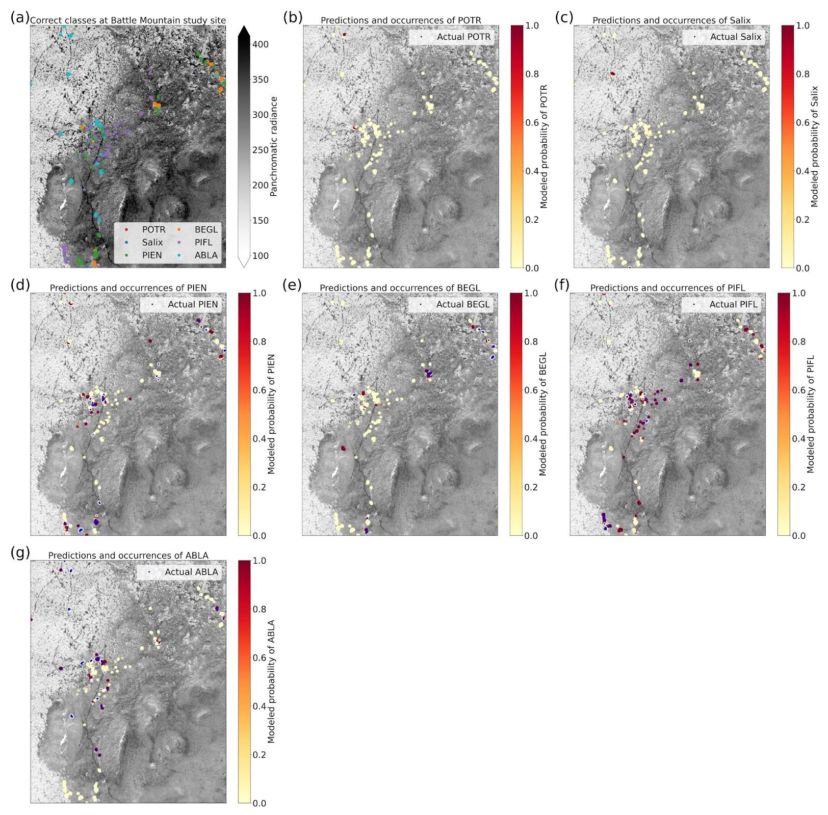
Figure D2 Targets and out-of-bag predictions for the 6-class model at the Battle Mountain study site. Formatting is explained in the caption of Fig. D1.

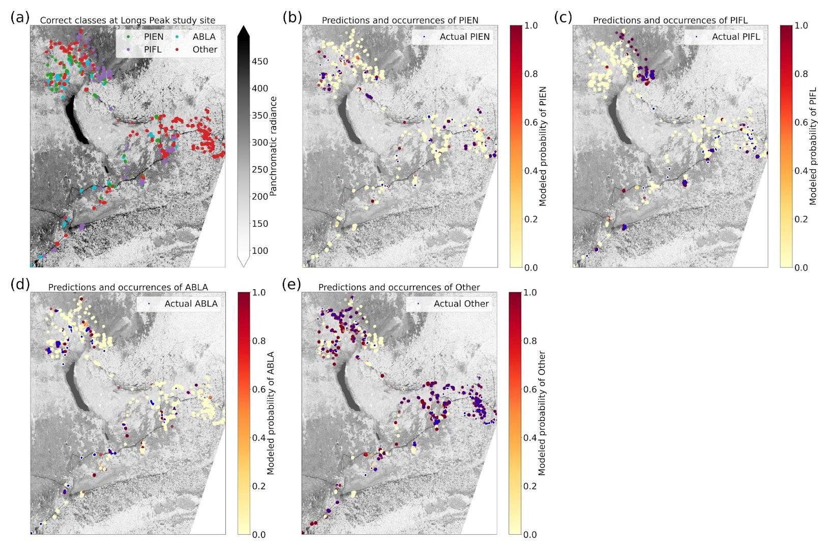
Figure D3 Targets and out-of-bag predictions for the 4-class model at the Longs Peak study site. Formatting is explained in the caption of Fig. D1.

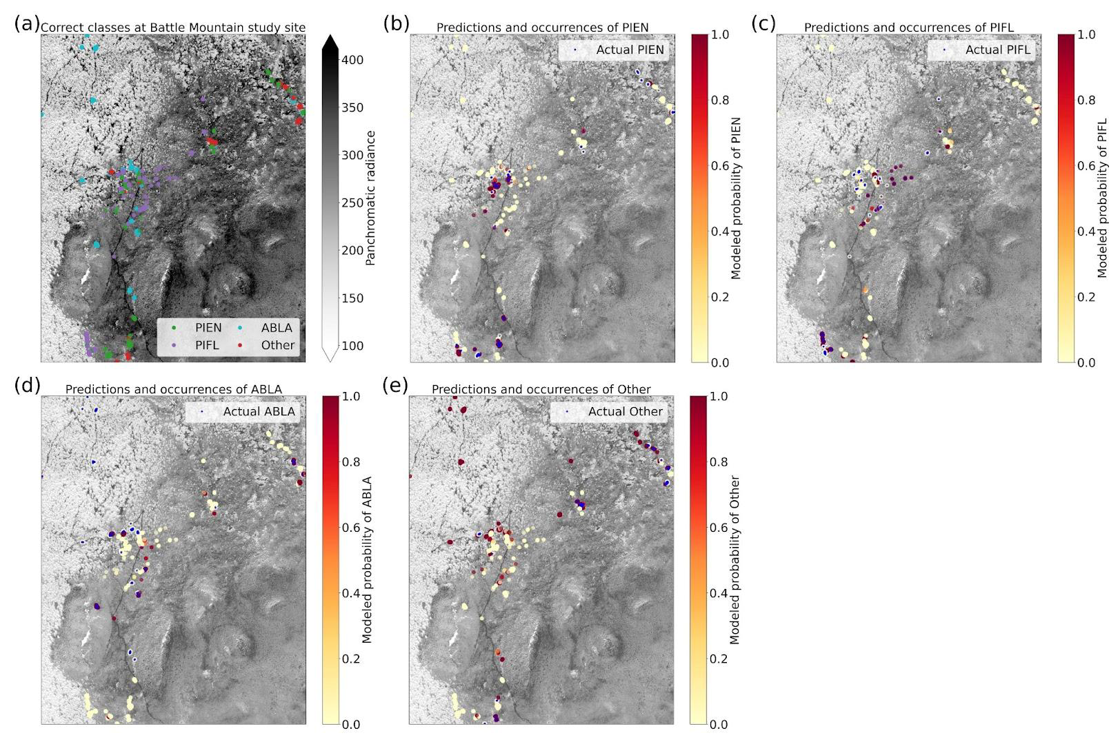
Figure D4 Targets and out-of-bag predictions for the 4-class model at the Battle Mountain study site. Formatting is explained in the caption of Fig. D1.

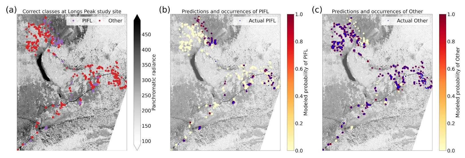
Figure D5 Targets and out-of-bag predictions for the 2-class model at the Longs Peak study site.  Formatting is explained in the caption of Fig. D1.

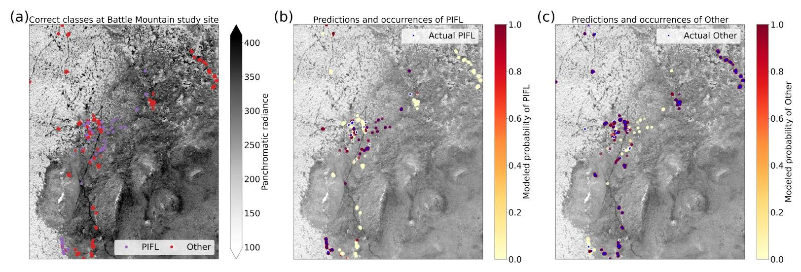
Figure D6 Targets and out-of-bag predictions for the 2-class model at the Battle Mountain study site. Formatting is explained in the caption of Fig. D1.