Multi-stress interaction effects on BVOC emission fingerprints from Oak and Beech: A cross-investigation using Machine Learning and Positive Matrix Factorization

Forest ecosystems are increasingly stressed through heatwaves, drought periods, and other factors such as ozone pollution or insect infestations. These stressors have a profound impact on the emissions of biogenic volatile organic compounds (BVOC) from trees, which in turn influence aerosol formation and atmospheric oxidation cycles and thus feedback on the atmospheric cleansing capacity and climate change itself. While previous studies have investigated the impacts of specific stressors on BVOC emissions, analyses of combined stress effects are rare, even though the stressors seldomly occur in isolation. This study investigates the impact of heat and (nighttime) ozone stress, both individually and in combination, on BVOC emissions from two ecologically significant temperate tree species: European beech (Fagus sylvatica L.) and English oak (Quercus robur L.). In a climate-controlled chamber, both tree species were subjected to heat stress (38 ± 3.3 °C) and ozone stress (∼ 120 ppb), separately and in combination. BVOC emission rates were measured using proton transfer reaction time-of-flight mass spectrometry, and the results were compared across pre-stress, heat, ozone, and combined heat-ozone conditions.

Heat stress elicited the strongest emission increases of isoprene, monoterpene, and green leaf volatiles in both species, while ozone suppressed the emissions of most BVOCs. Combined stress led to non-additive responses different from those in single-stress scenarios. Both machine learning and positive matrix factorization analyses were performed to identify key VOC fingerprint markers that may be applied to identify stress-impacted emissions from field data, and both methods showed good agreement. The OH reactivity of the emissions, which serves as a measure for their atmospheric chemistry and ozone formation impacts, was consistently highest under heat stress for both species. However, nighttime ozone stress led to reduced OH reactivity of emissions (by 10 %–18 %).

Our results underscore that the study of realistic combinations of stressors is crucial to understand future BVOC emissions and indicate that BVOC emissions could alter atmospheric chemistry and feedback with air quality and climate as heatwaves and pollutant-induced stress become more frequent due to climate change.

1 Introduction

The interaction between the atmosphere and forest ecosystems is crucial to understand, as it is an essential part of global biogeochemical and water cycles. A variety of atmospheric factors, including drought and increasing temperatures, can affect the integrity of the biosphere and its biodiversity (Pecl et al., 2017). However, the biosphere also has the capacity to influence the atmosphere (Arneth et al., 2010) by emitting various biogenic volatile organic compounds (BVOCs) from plants or soil (Pugliese et al., 2023). Every year, the terrestrial biosphere releases around 1000 Tg of BVOCs into the atmosphere (Guenther et al., 1993; Sindelarova et al., 2014), encompassing over 1700 identified organic compounds (Knudsen and Gershenzon, 2006) with diverse chemical properties and atmospheric lifetimes. BVOCs, being highly reactive, rapidly react with oxidant gases upon emissions, with lifetimes ranging from minutes (e.g., isoprene) to several days (e.g., methanol). The primary mechanisms of BVOC reactions involve the oxidation by hydroxyl radicals (OH) and ozone (O₃) (Finlayson-Pitts and Pitts, 1997). These processes have substantial implications for the formation of tropospheric ozone and secondary organic aerosols, subsequently influencing air quality, cloud formation and contributing to climate dynamics (Palm et al., 2018; Vella et al., 2023).

Over the past century, the global average temperature has risen by 1.5 °C (IPCC, 2023). With the recent intensification of global climate change, there has been a noticeable increase in the frequency and intensity of heatwaves worldwide (Pastor et al., 2024; Perkins-Kirkpatrick and Lewis, 2020). This trend is particularly pronounced in Europe (Rousi et al., 2022; Schuldt et al., 2020). Also, projections indicate that by 2100, the global temperature may further increase by 2–6 °C (Daussy and Staudt, 2020), and this warming will increase drought risk (Cook et al., 2018; IPCC, 2021). Consequently, this phenomenon not only directly impacts plant primary productivity but also has cascading effects on biogeochemical cycling processes within terrestrial ecosystems. As temperature (Roy et al., 2024) and soil water content are key drivers of plant metabolism, this anticipated climate change scenario is expected to heighten stress levels on plants (Jiang et al., 2019; Schuldt et al., 2020), leading to substantial changes in BVOC emissions. However, the overall direction of that change is to date uncertain, complicating BVOC predictions under future climate (Szopa et al., 2021) – one of the reasons for this uncertainty being the impact of climate-induced (combined) stressors.

Tropospheric O₃ concentrations are rising globally (0.5 %–2.0 % yearly). Climate change is also expected further to exacerbate ground-level O₃ at local and regional scales, increasing the frequency of high pollution days. Regions like Europe are likely to experience more elevated O₃ events (Royal Society, 2008). As a highly phytotoxic gas, O₃ significantly affects plant growth and development, with acute exposure causing necrotic damage and chlorophyll loss in leaves (Karnosky et al., 2007). To complicate matters, the interaction between O₃ exposure and trees is reciprocal (Paoletti, 2009): trees are affected by O₃, and influence O₃ levels in the air. Forest vegetation interacts complexly in regulating local tropospheric ozone concentrations, as trees can both scavenge and contribute to O₃ formation. The net effect depends on factors such as tree species, physiological status, environmental conditions, and air chemistry (Kivimäenpää et al., 2013; Pinto et al., 2010).

Plant-released BVOCs, significantly influenced by external factors (Fitzky et al., 2019; Darbah et al., 2010), are essential for intra- and interspecific communication (Heil and Karban, 2010), defense mechanisms against herbivores and pathogens (Dicke and Baldwin, 2010), and other biotic and abiotic interactions (Graham et al., 2024; Yu et al., 2022; Fitzky et al., 2019; Jud et al., 2016). These compounds primarily stem from metabolic processes from the leaf mesophyll tissues (e.g., mevalonate (MVA), methylerythritol phosphate (MEP), Lipoxygenase (LOX) or Shikimate pathway). More specifically, MEP and MVA are responsible for isoprenoid production (Bergman et al., 2024), including monoterpenes (MTs) and diterpenes, which contribute to thermal tolerance, whereas the LOX pathway is integral to green leaf volatiles production in response to mechanical damage or herbivory (Kutty and Mishra, 2023). While basic patterns of BVOC emissions in response to light and temperature are reasonably well understood and parameterized (Guenther et al., 2012), a large uncertainty around BVOC emissions is caused by the impact of stress. When plants undergo stress induced by factors such as drought, heat, herbivory, or elevated ozone levels, they can undergo fundamental changes in the composition and quantity of their emissions (Holopainen et al., 2018; Darbah et al., 2010). This introduces a notable challenge in accurately predicting BVOC emissions under varying stress conditions.

Under non-stressed conditions (i.e., constitutive emissions), plants typically invest a low amount of carbon, approximately 1 %–2 % of assimilated carbon (Fineschi et al., 2013), in BVOC emissions. However, during stress, emissions can increase significantly, sometimes exceeding the use of 10 % of the assimilated carbon (Niinemets et al., 2010). The response of plants to heat stress depends on the intensity of the temperature (Guenther et al., 1993). As a defensive mechanism, plants increase isoprenoid production, and it has been proposed that plant thermotolerance can be enhanced by protecting photosynthetic apparatus (Li and Sharkey, 2013; Sharkey, 2005). However, this mechanism remains debated: Harvey et al. (2015) showed that physiological concentrations of isoprene are likely too low to directly stabilize thylakoid membranes, while more recent work Zuo et al. (2025) suggests that isoprenoids may instead contribute to thermotolerance through signaling pathways (Ca²⁺-mediated) that regulate stress-responsive proteins, maintain photosynthetic efficiency, and induce heat shock responses. Also, heat stress can cause very high emissions of isoprene and monoterpenes by enhanced biosynthesis or increased vapor pressure of stored compounds (Werner et al., 2020) that the temperature-based models for constitutive emissions cannot explain (Nagalingam et al., 2023). High temperatures reduced the de novo emissions of certain BVOCs, particularly in conifers, where thermal stress amplifies the release of monoterpenes stored in resin ducts and induces the production of green leaf volatiles (Kleist et al., 2012). Numerous studies (Bourtsoukidis et al., 2012; Fitzky et al., 2023; Genard-Zielinski et al., 2018; Kivimäenpää et al., 2013, 2016; Kleist et al., 2012; Pikkarainen et al., 2022; Khedive et al., 2017) have emphasized that BVOC emission rates are species-specific and depend on external meteorological factors (such as soil moisture, temperature, and CO₂ concentrations). For example, higher sesquiterpene emissions were observed in Scots pine during heat stress (Kivimäenpää et al., 2016), whereas lower sesquiterpene and monoterpene emissions were found for European beech under heat stress (Kleist et al., 2012). From the drought and heatwaves experiments of Aleppo pine, Birami et al. (2021) showed that most BVOC emissions exponentially increased during the first heat wave. However, the emissions of monoterpenes and methyl salicylate showed reduced temperature sensitivity on the second heatwave.

Under O₃ stress, plants reduce O₃ influx into their tissue by regulating stomatal closure, mediated by calcium ions and hormonal signals (Guo et al., 2024). As O₃ induces the formation of reactive oxygen species (ROS), plants use enzymatic defenses (e.g., catalase, superoxide dismutase) to detoxify and mitigate lipid peroxidation in cell membranes (Feng et al., 2021). Also, it can activate the involved antioxidant enzymes gene expression (e.g., glutathione S-transferase, L-ascorbate peroxidase) (Baier et al., 2005) resulting in induced and modulated emission of BVOC. Studying Norway spruce, Kivimäenpää et al. (2013) found that a moderate temperature increase (∼ 1 °C above ambient) significantly enhanced BVOC emissions, especially monoterpenes and sesquiterpenes, but this effect was partially suppressed by elevated ozone levels (∼ 1.5× ambient). Elevated O₃ concentration (80 ppb) significantly increased the BVOC (mainly isoprene) emission rate of Chinese red pine (Xu et al., 2012). Moreover, Peron et al. (2021) found that isoprene emissions decreased while monoterpene and sesquiterpene emissions increased under combined drought and ozone stress in Oak. But under drought stress (without O₃), Fitzky et al. (2023) identified slightly elevated monoterpene and isoprene emissions from beech and oak.

Multiple abiotic and biotic stressors can interact in additive, antagonistic, or synergistic ways, modifying plant physiological processes and BVOC composition beyond single-stressor expectations. For instance, Lantz et al. (2019) have shown that the combined effects of elevated temperature and CO₂ on isoprene emission are highly interactive rather than independent: temperature exerts a dominant influence on emission rates, whereas elevated CO₂ can suppress isoprene production even in the triose-phosphate limitation. Likewise, exposure to multiple air pollutants or concurrent abiotic–biotic stresses (e.g., O₃ × herbivory) can trigger complex, non-linear responses that may enhance defensive signaling, alter stomatal conductance, and consequently modify volatile uptake and emission dynamics (Papazian and Blande, 2020; Yu et al., 2022). The overall impact of stress-induced changes in BVOC emissions still remains elusive, specifically under multiple stressors (Yang et al., 2025), as the effect of blending two stressors, like heat + O₃ or O₃ + elevated CO₂ is not well-understood (Holopainen et al., 2018), and responses may vary between species, as we discussed.

Therefore, this study specifically aimed (1) to investigate BVOC emission patterns from both tree species under heat or ozone and combined stress in controlled environmental conditions, (2) to identify specific stress marker BVOCs for beech and oak for the identification of stress-induced BVOC emissions in future field measurements, (3) to estimate the potential atmospheric impact of changing emission patterns in terms of OH reactivity as an indicator for ozone formation potential. We applied stressors sequentially on the same individuals to simulate realistic environmental stress storylines.

2 Materials and methods

2.1 Experimental set-up

2.1.1 Plant chamber and stress treatment

The experiment was carried out in PLUS (Plant Chamber Unit for Simulation) which can be coupled to the atmosphere simulation chamber SAPHIR (Simulation of Atmospheric PHotochemistry In a large Reaction Chamber) at the Forschungszentrum Jülich, Germany, during the spring, 2024. This study focuses on direct plant emission measurements obtained from the PLUS chamber (Fig. 1a). Emissions were introduced to SAPHIR for ixidation experiments that will be subject of a future analysis. The PLUS plant container is a custom-build, gas-tight, temperature- and light-controlled container that can house up to six tree-type plants. Inside the chamber, a rectangular aluminum frame supports a 9.32 m³ Teflon film enclosure containing the upper portions of potted trees. This enclosure separates the soil from the stems and the leaves of the trees. PLUS operates in a dynamic flow-through mode using a turbulent airflow of 100 L min⁻¹ of synthetic air that passes through the Teflon enclosure, ensuring homogeneous, steady-state conditions inside the chamber. Important environmental factors within the PLUS chamber, such as temperature, photosynthetically active radiation (ranging from 0 to 800 µmol m⁻² s⁻¹ at a distance of one meter), and soil moisture, were controlled (Hohaus et al., 2016). After installation of the experimental saplings, the PLUS Teflon enclosure was kept at a slight overpressure of approximately 35 Pa to prevent any trace gases from diffusing into the enclosure. The synthetic air was mixed with 400 ppm CO₂ to maintain levels necessary for plant photosynthesis. More details about the functional and structural description can be found in Hohaus et al. (2016).

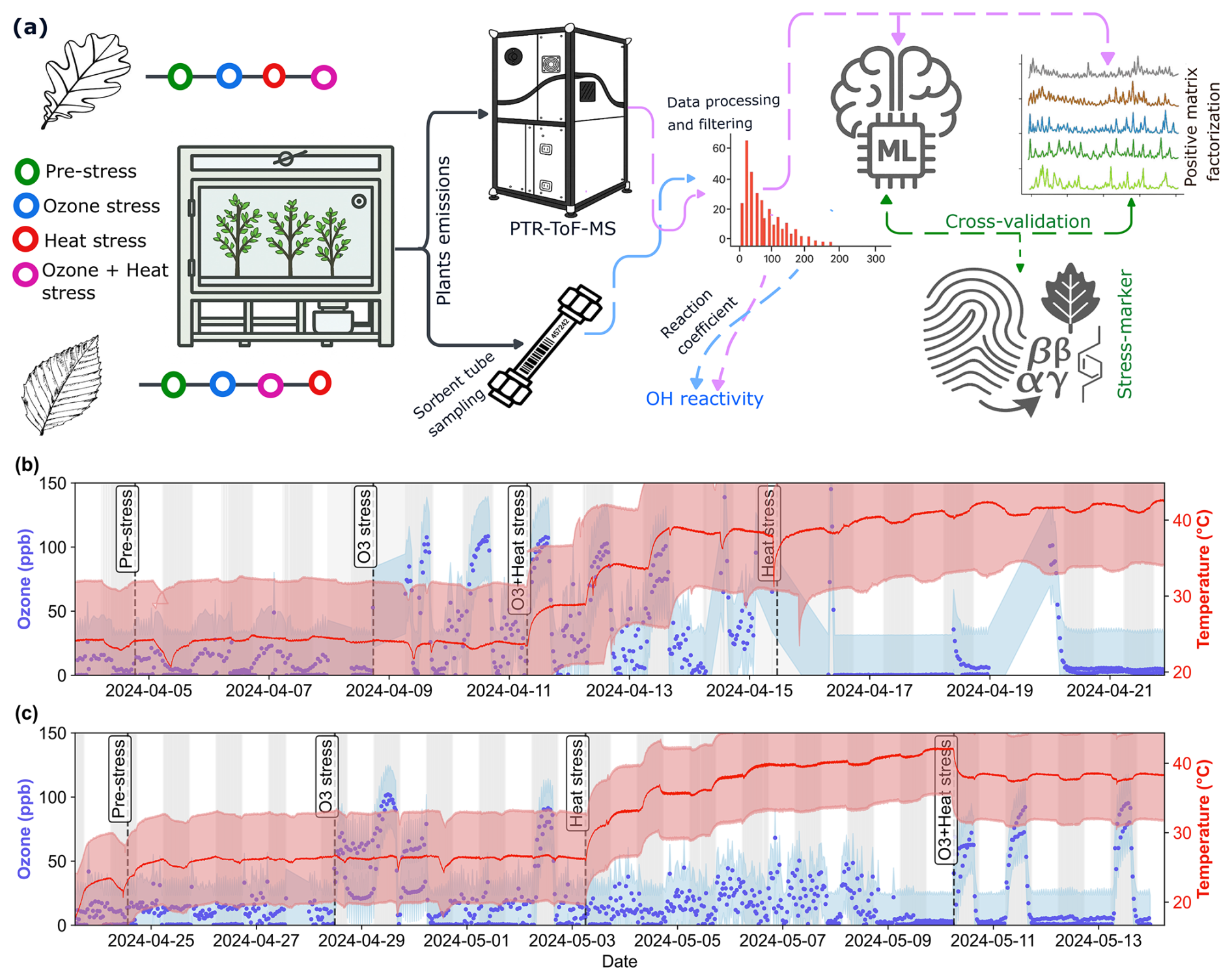
Figure 1 Overview of experimental design and stress timeline for beech and oak. (a) Schematic illustration of the experimental setup, data processing and analysis pipeline, (b, c) time series of ozone concentration (blue) and temperature (red) during pre-stress and stress phases for beech (b) and oak (c). The experiment is divided into four consecutive phases: Pre-stress, O₃ stress, Heat stress, and O₃ + Heat stress, indicated by vertical dashed lines. White and grey background areas represent day and night periods, respectively. Shaded regions around lines represent the standard deviation from the mean ozone concentration and temperature.

Experiments were conducted with the two major broadleaf forest tree species in Germany: Quercus robur L. (English oak) and Fagus sylvatica L. (European beech). Before the experiment, 24 saplings of ∼ 1.4 m in height of beech (12 individuals) and oaks (12 individuals) were selected under conditions ensuring they were disease- and pest-free, had straight stems, and were overall healthy. The plants were kept in a greenhouse under near-ambient light conditions with photosynthetically active radiation. During this period, they were watered regularly. To quantify the total leaf area of each plant, all leaves were photographed against solid blue backgrounds at known distances and scales right before installing them in the plant chamber. Four images were taken from different angles for each individual to reduce bias. Then we processed these images using the ImageJ software according to Schneider et al. (2012), to extract the leaf area, and estimated total leaf area using the geometric means.

The stress treatments were applied sequentially on the same set of individuals to simulate realistic environmental scenarios (“storylines”). This experimental approach was designed to reflect natural conditions, where trees in the same landscape may experience heatwaves and ozone pollution either simultaneously, sequentially, or in varying order.

The first experiment was conducted with beech trees from 3 to 23 April 2024 (Fig. 1b). Six trees were selected from the 12 available and placed into the plant chamber. Stems were sealed with Teflon foil to isolate the canopy from the soil. One beech branch had to be cut for the tree to fit into the chamber, potentially impacting emissions in the first days of the experiment. The first 24 h after setting up the experiment were considered the plant adaptive period, and data from this period were excluded from the analysis. Oak experiments were conducted in a similar fashion from 24 April 2024 to 13 May 2024, using the six healthiest individuals (Fig. 1c).

Following the pre-stress period, ozone, ozone + heat, and solely heat stress were periodically induced on the beech trees. For heat stress experiments, temperature was gradually increased (Fig. 1b, c) and ozone was (except for two days for the oak experiment, Fig. 1c) applied during the night cycle. The reason for this approach was twofold: On the one hand, this approach avoided reactions of emitted terpenoids with ozone during the day, when emissions are highest, which would interfere with quantifying primary BVOC emissions because it would produce oxygenated VOC products. For later analysis of BVOC emissions we excluded data from nights and from the two days where ozone was applied, to avoid ozone impacts on the observed VOCs. In addition, this allowed us to study the understudied phenomenon of nighttime ozone exposure of trees. Previous studies (e.g. An et al., 2024; He et al., 2022; Musselman and Minnick, 2000), have reported that certain areas can experience relatively high ozone concentrations at night, while plants can be more susceptible to ozone stress at night than during the daytime because they have lower defenses at night (Musselman and Minnick, 2000).

The ozone concentration in both experiments ranged from 0 to 120 ppb. During nighttime ozone stress and ozone + heat stress, ozone concentrations were 90 ± 21.5 and 93.1 ± 19.6 ppb, respectively. Soil moisture was maintained at 50 %–80 % (relative sensor readings) with air temperatures ranging from 20 to 44 °C. When no heat stress was applied, air temperature was 25.9 °C (±0.6 °C). During heat stress and combined stress, it was 38 ± 3.3 and 38.1 ± 0.4 °C, respectively. The applied heat stress was selected to simulate ecologically realistic and physiologically stressful conditions comparable to recent Central European heatwave events, where canopy temperatures frequently exceed 35–40 °C (Schuldt et al., 2020). Light conditions remained constant during the day (UTC (coordinated universal time) 16:00–06:00), with lights turned off at night (UTC 06:00-16:00). At the end of the experiments (after ozone + heat stress), the plants had wilted.

2.1.2 VOC emission measurements: PTR-ToF-MS

Air was sampled from the SAPHIR-PLUS chamber through a thermally insulated and heated $\mathrm{1}/\mathrm{4}$” (0.635 cm) PFA line with a flow rate of ∼ 3 L min⁻¹. Real-time BVOC signals were measured using a proton transfer reaction time-of-flight mass spectrometer (Vocus PTR-ToF-MS, Krechmer et al., 2018) with a 1 s time resolution. The PTR-ToF-MS was operated with a drift tube temperature of 100 °C, a drift voltage of 600 V, and a drift pressure of 2.5 mbar in proton transfer ionization (H₃O⁺) mode. Mass resolution of the instrument was around 8000.

A gas standard mixture containing 19 compounds with masses ranging from 33 amu (atomic mass unit) to 671 amu (Table S1, in the Supplement), that was calibrated against a gravimetrically prepared, certified standard, was used for regular calibrations. PTR-ToF-MS data was processed using Tofware. A mass list was prepared with 500 compounds for both experiments from a mass-to-charge ratio ($m/z$) range of 18 to 450 amu (details in supplementary data, sheet “Identity_mz”). Zero air measurements were conducted hourly and used for background subtraction.

Sensitivities for compounds not included in the gas standard were estimated using a theoretical calibration method according to Cappellin et al. (2012). This involved fitting a sigmoidal function, which reflects the expected transmission characteristics of a Vocus-PTR-ToF-MS after dead time correction, to the reaction-rate-normalized sensitivities of VOCs that were calibrated using the gas standard and are known to not fragment or cluster (Jensen et al., 2023; Pfannerstill et al., 2023). Emission rates were calculated from such derived concentrations using the chamber flow rate and the leaf area (Edtbauer et al., 2021).

To ensure quality and reliability, emissions data were filtered using a systematic signal-to-noise ratio (SNR) approach. For each compound, the SNR was calculated as the ratio of its measured emissions to its corresponding LOD value at each time point. Compounds were selected whose SNR was greater than or equal to 3 for at least 30 % of the time series. Compounds that did not meet both the SNR threshold and the minimum temporal coverage requirement were excluded from further analysis. Applying the SNR threshold, 80 and 82 VOC species for beech and oaks were selected, respectively. The uncertainties in both the theoretical and gas-standard calibrations were assessed based on average estimates. For the theoretical calibration, the uncertainty was estimated at 51.3 %, while the gas-standard calibration uncertainty, consisting of the calibration standard uncertainty and the mass flow controller uncertainty, was estimated at 10 %.

Exact masses and attributed chemical formulas are reported. Attribution of compound names to chemical formulas was performed to the best of our knowledge, however, identification is tentative because the PTR method cannot distinguish isomers and is subject to fragmentation.

2.1.3 Terpenoid composition: GC-MS

The PTR-ToF-MS method (Sect. 2.1.2) identifies exact masses of compounds which can be attributed to a chemical formula but cannot separate isomers. Structural identification of mono- and sesquiterpenes was performed by sampling onto stainless steel tubes (Markes International Limited, England) packed with Tenax TA (porous organic polymer) and Carbograph 1TD (graphitized carbon black) sorbents.

Sorbent tube sampling was performed with a modified MTS-32 autosampler (Markes International Limited, England), which was directly connected to the PLUS via a PFA line. The autosampler consists of a stainless steel manifold block, timer, mass flow controller, vacuum pump (Laboport N86 KT.18, KNF, France), and a copper ozone scrubber treated with potassium iodide. Sorbent tubes were fitted with diffusion locking caps (Markes International Limited) to prevent contamination. Flow rates during sample collection varied from 50 to 300 mL min⁻¹ due to technical constraints of the autosampler, with 300 mL min⁻¹ occurring during the oak experiment's pre-stress and ozone exposure phases. However, this variation is not likely to affect the results. After sampling, sorbent tubes were sealed with brass storage caps and stored at 4 °C until analysis.

Analysis of the sorbent tubes was performed with an Agilent gas chromatograph coupled with a mass spectrometer (7890A GC–5975C inert MSD, Santa Clara, USA). Sorbent tubes were thermally desorbed at 250 °C for 10 min (TD100-xr, Markes International, Llantrisant, UK) and cryofocused at 10 °C, before being transferred to the GC–MS system through a capillary column at 160 °C. An HP-5MS capillary column (50 m × 0.2 mm × 0.33 µm, Agilent Technologies, Santa Clara, USA) was used to separate the VOCs with a carrier gas flow of 1.2 mL min⁻¹ of helium. The oven program used an initial temperature of 40 °C for 3 min, before ramping at 5 °C min⁻¹ to 210 °C, and again at 20 °C min⁻¹ to 250 °C, and a final hold of 8 min to give a total runtime of 47 min. The ion source and quadrupole temperatures were held at 230 and 150 °C, respectively. No-injection column blanks and empty stainless-steel cartridges (containing no sorbent material) were run periodically alongside the samples to provide an indication of background contamination arising from the analytical system (e.g., siloxanes, phthalates). Travel blanks (unopened, pre-cleaned sorbent cartridges that travelled to and from the field site alongside the sample tubes) were also analysed.

Chromatograms from the GC-MS laboratory analysis were processed using the PARADISe V.6.1 software (Quintanilla-Casas et al., 2023). Compounds were identified based on pure standards and tentative identification based on matches with the NIST 2023 Mass Spectral Library (National Institute of Standards and Technology, Gaithersburg, MD, USA). Compounds with a match factor above 800 and probability above 30 were accepted, as well as compounds with 3 hits of the same structural formula. Incompatible compounds were manually assessed and identified by structural formula or probable matches. Concentrations were quantified using the external standards. In the cases of unavailable standards, the closest structurally related standard compounds were used. Contaminant compounds that are known to arise from plastics (e.g., phthalates) from storage or transport or from column degradation (siloxanes), were excluded from the dataset.

Identification of mono- and sesquiterpenes from GC-MS data was used to calculate OH reaction rates for the average isomeric composition for each experiment phase. Species-stress-specific OH reaction rate coefficients are available in supplementary data. Only daytime emission data were used to account for both de novo and stress-induced BVOC emissions.

2.2 Integrated analytical approach

BVOC emissions in response to stress are not static; they change over time as the stress persists or alleviates. Also, plants might start emitting a particular compound as a response to an initial stress signal, and the concentration might increase, decrease, or change composition, with many different compounds being emitted simultaneously as the stress continues. Given this complexity, classical statistical methods are limited unless the underlying relationship between variables is understood or predefined. In contrast, advanced algorithms (e.g, machine learning, positive matrix factorization) excel in uncovering complex, nonlinear patterns without requiring explicit assumptions about variable interactions. Therefore, machine learning (ML) and positive matrix factorization (PMF) were used to comprehensively analyze BVOC stress fingerprints (Fig. 1a).

A supervised ML model classified four treatment categories: pre-stress, ozone stress (nighttime), heat stress, and ozone + heat stress, based on consecutive emission profiles. To interpret the model's decision-making process and identify the important features, SHapley Additive exPlanations (SHAP) were used. SHAP analysis enabled features or BVOC compound-level interpretability by indicating whether high or low emissions of individual VOCs contributed to specific stress classifications, thereby providing both directionality and diagnostic specificity.

In parallel, PMF, an unsupervised source apportionment method, extracted latent emission profiles and their temporal dynamics. PMF resolved the VOC emissions into co-varying compound groups (factors) corresponding to physiological responses (e.g., early heat stress, oxidative damage, late heat stress, etc.). PMF and ML offer complementary perspectives: PMF elucidates temporal emission patterns, whereas ML identifies the most informative features for distinguishing stress types. The comparison between results from ML and PMF thus allows for higher certainty in fingerprint identification than one single method would provide.

2.2.1 Machine learning model: Random Forest

Time-resolved VOC measurements from beech and oak experiments under four stress conditions were used to train a machine learning model for classifying stress conditions (Fig. 1). It contains 20 min resolution daytime VOC data over the 2 months (Figs. S5a and S6a in the Supplement) containing the emission rate of each VOC, stress label, and time. A structured preprocessing pipeline was applied to ensure the integrity of the input data and enhance model performance. First, the dataset was checked for invalid measurements in VOC emission features; no missing, null, or zero values were found. Then, variance-based filtering was applied to remove quasi-constant features to reduce redundancy and exclude non-informative VOCs. Subsequently, correlation was checked between the features (by Pearson correlation). Features showing absolute correlation coefficients greater than 90 % were flagged and reviewed individually. Known fragment or water cluster ions were removed. For instance, isoprene (C₅H${}_{\mathrm{9}}^{+}$) correlated with an r² of 0.93 with C₃H${}_{\mathrm{5}}^{+}$, which represents a known fragment ion rather than a distinct compound. Subsequently, a logarithmic transformation was applied to reduce skewness, scale down extreme flux magnitudes, and improve distribution symmetry. To normalize feature scales and stable model optimization, the log-transformed data were standardized.

The dataset was split chronologically into training and test subsets for model training using a stratified temporal splitting approach (Figs. S5c and S6c). Within each stress class, 70 % of the earliest samples were allocated to the training set and 30 % to the test set. This approach ensured temporal separation between training and test periods, also a balanced representation of all classes (Figs. S5b and S6b). An alternative configuration was used as a sensitivity check in which an equal number of samples were randomly selected from each day and assigned to the training and test sets. No substantial differences in model performance were observed between the two approaches.

A random forest (RF) model was used to classify stress due to its robustness, interpretability, and ability to handle structured data. The implementation followed the scikit-learn python framework (Pedregosa et al., 2012) for machine learning. A hyperparameter optimization step was performed using grid search to tune the number of trees, maximum tree depth, minimum number of samples per split, and minimum number of samples per leaf. The optimization was carried out using 3-fold cross-validation with the weighted F₁ score as the evaluation metric. Model performance was recorded across all parameter combinations, and the one with the highest validation score was selected for the final model fitting.

Robustness of the model was evaluated through a non-parametric bootstrapping procedure over 1000 iterations. Test predictions were resampled with replacement to recalculate accuracy and weighted F₁ scores in this process. Kernel density estimation was then applied to evaluate uncertainty and performance variability. For predictive uncertainty, Shannon entropy was calculated from the class probability outputs of the random forest for each test observation. Samples with higher entropy values corresponded to greater uncertainty in the predicted class. The distribution of entropy values was analyzed across prediction accuracy (correct vs. incorrect) and further assessed within each stress category. Also, time series analyses were conducted to illustrate temporal dynamics in prediction confidence.

To determine feature importance and interpret the model's predictions, SHapley Additive exPlanations (SHAP, Lundberg and Lee, 2017) was used with the TreeExplainer method. This is a game-theory based approach that attributes the output prediction of a model to its input features, providing an interpretable solution of feature importance that is both local (according to stress type) and global (in overall model for all stress conditions). SHAP values were calculated for all samples in the test set and then combined to create class-specific feature importance rankings. The top 15 VOC features with the highest mean absolute SHAP values were identified for each stress condition. Pairwise comparisons were performed to evaluate feature redundancy and specificity across classes, and the overlaps and unique features were examined. Finally, potential stress-related chemical fingerprints were identified after using the SHAP values and their influence on the predictions for that specific stress.

2.2.2 Positive matrix factorization

To cross-investigate the random forest outcomes, we performed PMF analysis on VOC species measured by the Vocus-PTR-ToF-MS. The PMF model was used to identify the VOC time series into factor profiles, factor time series, and residuals, thereby isolating characteristic stress-related emission patterns. The PMF model has been widely applied to identify different sources and chemical processes of VOCs measured by PTR-ToF-MS across anthropogenic to biogenic emissions (Bhattu et al., 2024; Gkatzelis et al., 2021; Song et al., 2024). The analysis was conducted separately for beech and oak using the Multi-linear Engine (ME-2) and implemented via the Source Finder (SoFi) package (version 8.6.4.4) with Igor-Pro software (version 9.05). The bilinear PMF model resolved the sample matrix into two non-negative matrices: factor profiles (F) representing characteristic mass spectra and factor contributions (G) representing the temporal evolution of each profile, with an associated residual matrix (E).

The cleaned dataset was used as the data matrix, and error matrices were created by 15 % of the measured concentration, combined with twice the standard deviation observed during periods when the signal remained stable. Before selecting the final factor solution, we went through multiple checks: we checked whether the factor's time series appeared random or lacked a clear pattern, inspected the y axis to determine if the factor's contribution was small or noisy, and checked correlation of the factor's time series with main compounds. We also checked the explained variation to identify which compounds were most strongly linked to each factor. Finally, we looked at the time series of those compounds to assess whether they appeared random or noisy.

Results from PMF (top 15 compounds) and ML-based SHAP (top 15 compounds) analyses were integrated as cross-investigation for comprehensive fingerprint identification. Taken together, the integration of PMF and SHAP results extends the understanding of VOC emission tracers under stresses shown in Sect. 3.6.

3 Results and discussion

3.1 Species and stress matter: Beech vs Oak behave differently beyond additive reaction to combined stressors

Isoprene (C₅H${}_{\mathrm{9}}^{+}$, $m/z$ 69.069) emissions were influenced by various stress conditions, with the highest emissions observed under heat stress for both species (Fig. 2). Under pre-stress (acclimation) conditions, the emission rate for beech was 0.003 (±0.0006, standard deviation) nmol m⁻² s⁻¹, i.e. close to zero, as expected (Karl et al., 2009; Moukhtar et al., 2005). Under heat stress, beech switched from a low/non-isoprene emitter to an isoprene emitter, rising to 0.22 (±0.08) nmol m⁻² s⁻¹ (Fig. 3a). This could be a strategy to increase thermotolerance (Sharkey et al., 2001), as beeches are more sensitive to heat stress than oaks (Raftoyannis and Radoglou, 2002). Nighttime ozone stress, on the other hand, led to a reduction in isoprene emissions in beech, consistent with Feng et al. (2019), who reported an 8 % decrease in isoprene emissions under elevated ozone levels. Under combined stress, isoprene emissions increased moderately (to 0.01 nmol m⁻² s⁻¹) for beech, while oaks showed significantly lower emissions under this condition. Despite the reduction caused by heat and ozone stress, oaks still emitted more isoprene than beeches overall (Fig. 2b). Under combined stress, isoprene decreased significantly, which may be a compensatory response. This trend is also observed in Arctic regions (Rinnan et al., 2020) and temperate forests (van Meeningen et al., 2016, 2017). That compensatory isoprene response could be part of a broader stress-signaling and recovery system (Jud et al., 2016). More recent evidence suggests its role extends beyond physical membrane stabilization, involving phosphorylation-mediated signaling and regulation of chloroplast movement and stress-responsive proteins (Weraduwage et al., 2024).

The terpenoid emissions varied substantially depending on the stress, and species. Since PTR-MS cannot distinguish between different mono- and sesquiterpene isomers, we here discuss the sum of all C₁₀H₁₆ compounds as monoterpenes (MTs) and the sum of C₁₅H₂₄ compounds as sesquiterpenes (SQTs), while changes in composition of MT and SQT emissions are discussed below. Monoterpene emissions in beech increased substantially under O₃ + heat stress (↑728 %) (Fig. 2). Beech sesquiterpene emissions decreased across all stress conditions (↓84 % under heat), because we induced elevated sesquiterpene emissions pre-stress through cutting a branch. Therefore, this result cannot be generalized. However, a temperature-dependent increase is expected, as shown and parameterized for beech by Moukhtar et al. (2005). Monoterpene emissions from oak were substantially increased by heat stress (88 %) and slightly reduced by nighttime ozone (24 %) and combined stress (17 %). Pinto et al. (2010) warned that emissions could be underestimated due to the rapid reactions between ozone and MTs, which may mask the true extent of chemical defenses. This issue was alleviated here by applying ozone stress exclusively during plants' nighttime, flushing out residual ozone in the morning, and reporting the daytime emissions that followed the nighttime stress.

Oaks' SQTs emissions substantially increased (0.022 nmol, 430 % compared to acclimation) under heat stress. Ozone and combined stress inhibited SQT emissions by ∼ 50 % compared to pre-stress conditions in both species. While oxidative stress can sometimes induce SQT emissions, some studies (Vo and Faiola, 2023) have reported a decrease in emissions with ozone exposure. For protection against ozone stress, not the amount but the ozone reactivity of the emissions is decisive (Sect. 3.3). It is important to note that stress response is usually non-linear and depends on factors such as dose levels. A study on a Central European spruce forest (Bourtsoukidis et al., 2012) found that temperature is a key driver of sesquiterpene emissions in moderately polluted environments, but when ozone levels surpass a critical threshold, emissions are more closely linked to ozone concentrations.

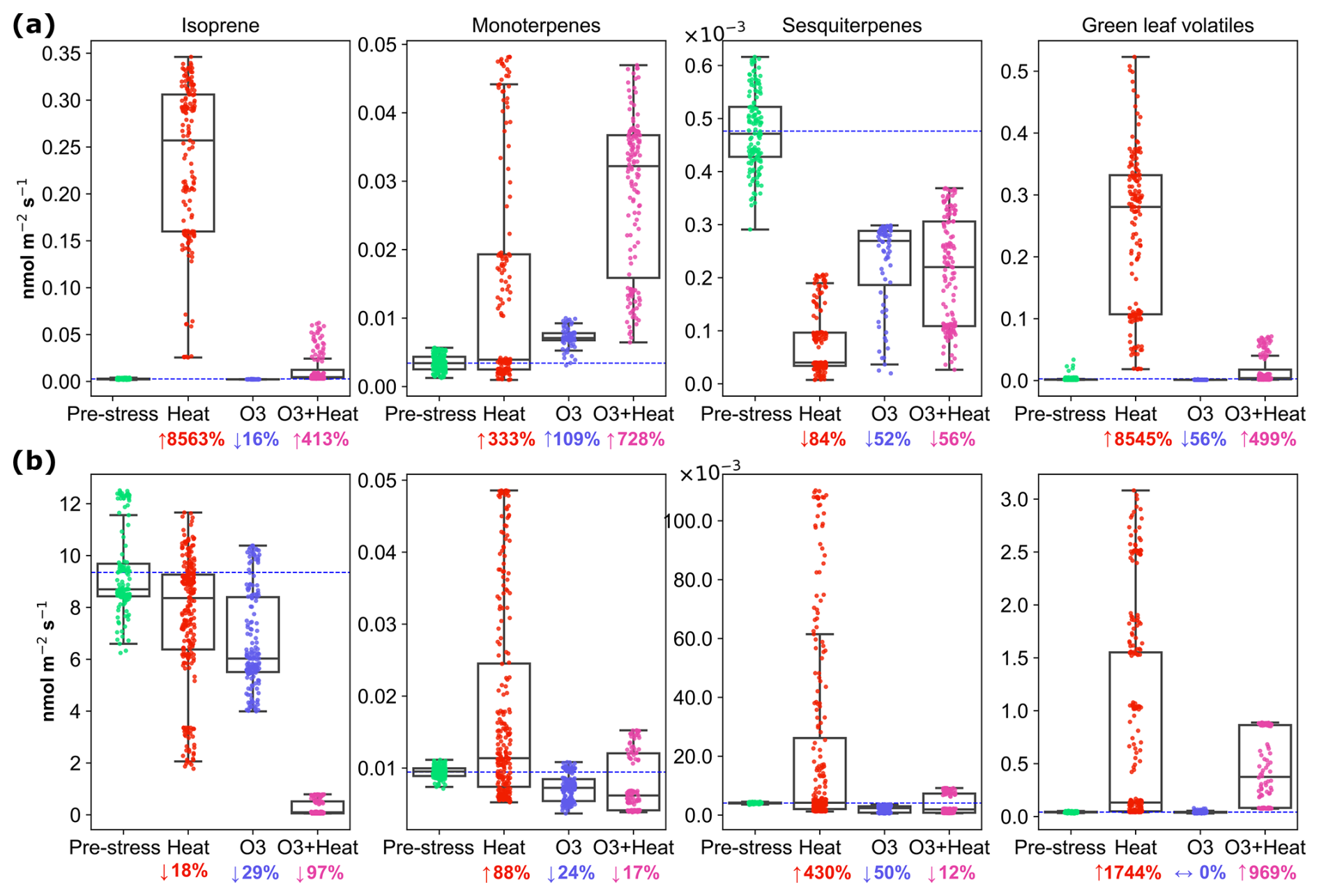
Figure 2 Emissions of isoprene, monoterpene, sesquiterpene, and green leaf volatile emissions from (a) beech and (b) oak under pre-stress, heat, O₃, and combine stress (O₃ + heat) conditions. Boxes represent interquartile ranges, horizontal lines indicate medians, and whiskers show the data spread. The dashed horizontal blue line represents the average pre-stress emission level for reference. Percent changes compared to average pre-stress levels are indicated by ↑ = increase, ↓ = decrease, ↔ = no change.

Green leaf volatiles (GLVs) were substantially increased by heat stress and less by combined stress in both species, while nighttime ozone stress barely affected the green leaf volatiles. This aligns with previous studies, which have demonstrated that GLVs are rapidly emitted in response to increased metabolic activity under high temperatures (Cofer et al., 2018; Jardine et al., 2015; Rieksta et al., 2023).

Table 1 Percentage change in emission rates of volatile organic compounds under four biosynthetic pathways, MEP (Methylerythritol Phosphate), LOX (Lipoxygenase), SKP (Shikimate), and MVA (Mevalonate) in beech and oak for three stress conditions. Sign (+/−) indicate increases or decreases in emission relative to the pre-stress baseline (set at 0 %). Superscript letters (a–d) denote statistically significant differences within each row, with different letters indicating significant variation among stress events (p<0.05).

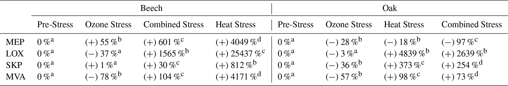
Compounds tentatively identified from PTR-ToF-MS measurements were assigned to pathways based on their known biosynthetic origins or related to pathways adapted from Fitzky et al. (2023) (Table 1). These were used to estimate shifts in major plant biosynthetic pathways (LOX, MEP, MVA, and SKP) under different stress conditions. The single and combined stress treatments showed the fundamental differences in how each species reacts to abiotic stress. During heat and combined stress, compounds related to MEP and SKP pathways (Fitzky et al., 2023) were increased, e.g., isoprene, monoterpenes, benzaldehyde (C₇H₇O⁺, $m/z$ 107.05) and phenethyl acetate (C₁₀H₁₃O${}_{\mathrm{2}}^{+}$, $m/z$ 165.091) (Table 1). Based on these observations, beech activated the plastid-localized metabolic pathways, particularly the MEP and SKP pathways, under both heat and combined ozone-heat stress (Table 1). Stress induced high isoprene and monoterpene emissions (Fig. 2a) under heat and combine stress, possibly by increased enzyme synthesis or accumulation of dimethylallyl diphosphate and geranyl diphosphate (Nogués et al., 2006), indicating a chloroplast-centric metabolic shifting to an active investment in photoprotection (Peñuelas and Munné-Bosch, 2005), redox homeostasis (Loreto et al., 2004), and antioxidant defense (Singsaas, 2000). Notably, while beech also showed substantial increases in emissions from cytosolic pathways (MVA and LOX), including acetaldehyde (C₂H₅O⁺, $m/z$ 45.03), hexanal (C₆H₁₃O⁺, $m/z$ 101.09), C₆H₁₁O⁺ (hexenal, $m/z$ 99.08), hexanol fragment (C₆H${}_{\mathrm{13}}^{+}$, $m/z$ 85.10) these appeared to be part of a broader, integrated metabolic adjustment, coordinated with plastidial pathways (MEP and SKP), following a diel cycle (Figs. 3a, c) contributing a balanced physiological response rather than a primary damage response.

Oak showed a different physiological strategy. Sesquiterpenes, hexenyl acetate (C₈H₁₅O${}_{\mathrm{2}}^{+}$, $m/z$ 143.10), acetaldehyde, hexanal and other compounds (Table A2) related to LOX and MVA pathways increased significantly during heat stress and under combined stress (except SQTs). The overall LOX and MVA pathway shift during those stressors is significant (Table 1). This points to a more cytosol- and membrane-centric defense mechanism (LOX, MVA) by a dominant activation of the LOX pathway particularly under heat and combined stress. Sesquiterpenes are the primary products of MVA, which significantly increased by heat (Fig. 2b) and are associated with membrane lipid peroxidation (Lõpez et al., 2011) and rapid oxidative signaling (Basile et al., 2025).

The VOC response to nighttime ozone alone was relatively low compared to heat or combined stress in both species, likely due to limited stomatal uptake during nighttime exposure, resulting in a weaker trigger of VOC biosynthesis (Table 1), unless combined with additional stressors (i.e., heat). Several studies have shown that plants can recover from ozone stress within 24–72 h, depending on the species (Kanagendran et al., 2018; Velikova et al., 2005). While this recovery potential may have moderated the observed ozone response, it also provided an opportunity to capture ecologically realistic post-exposure dynamics. The exposure to nocturnal ozone reflects ecologically relevant conditions, as recent studies have reported frequent nocturnal ozone events, where ozone concentrations remain elevated or even increase at night due to residual layer mixing and limited nighttime deposition (Musselman and Minnick, 2000; An et al., 2024), especially in mountainous areas such as most of German forests. Although stomatal conductance is generally lower at night, it is not negligible, and nocturnal ozone flux into leaves can still occur, potentially leading to oxidative stress when plant defense capacity is reduced (Musselman and Minnick, 2000). It has been reported that trees in regions with high ozone levels can have stomata open at night (Caird et al., 2007).

Peron et al. (2021) observed in oak that the combination of ozone with drought altered VOC emission profiles and led to opposing feedback compared to ozone alone. While ozone-induced oxidative stress can stimulate VOC emissions, the magnitude and composition of these emissions are highly dependent on factors such as plant species, developmental stage, stress severity and environmental conditions (Pinto et al., 2010; Renaut et al., 2009), emphasizing the complexity of plant responses to ozone. Mechanistically, ozone exposure leads to intracellular Reactive Oxygen Species (ROS) accumulation and the activation of stress signaling compounds (e.g. jasmonic acid) (Kangasjärvi et al., 2005). Furthermore, chronic ozone exposure leads to downregulation of photosynthetic enzymes such as RuBisCO (Pelloux et al., 2001), suppression of carbon fixation, and activation of offset metabolic pathways including phosphoenol pyruvate carboxylase (Gaucher et al., 2006) and the pentose phosphate pathway (Dizengremel et al., 2008). This metabolic shifting may further constrain VOC production under ozone.

Implementing stress sequentially on the same individuals may have carry-over or “lingering” effects from prior stress (Kleist et al., 2012) and represents as such a realistic scenario that a tree may experience in an ecosystem. However, this non-traditional approach makes the results of each stress scenario linked to the previous sequence and thus not generalizable on their own. Recent studies showed that repeated or sequential stress exposure can induce a form of physiological stress memory, wherein plants retain molecular or metabolic imprints that influence subsequent responses (Fleta-Soriano and Munné-Bosch, 2016; Liu et al., 2022a). Such memory arises through transient chromatin modifications, persistent activation of defense-related genes, and metabolic reprogramming that can enhance or attenuate volatile production upon re-exposure (Ding et al., 2012; Xin and Browse, 2000). For instance, Blande et al. (2014) highlighted that prior oxidative or thermal stress may reallocate carbon and energy resources, altering precursor availability for VOC synthesis, leading to reduced emissions under prolonged exposure but more rapid or efficient activation during mild re-exposure.

3.2 Plants' stress-induced diel emission dynamics

Under pre-stress conditions, terpenoid emissions, specifically monoterpenes (MTs) and sesquiterpenes (SQTs), followed the expected diel cycle, with emissions peaking during the light period and falling at night (Fig. 3), consistent with their strong dependence on light. This pattern aligns with established findings that emission rates are modulated by environmental variables such as temperature and light (Guenther et al., 1995). However, exposure to abiotic stressors, particularly heat and the combination of ozone and heat, results in the loss of their distinct diel behavior. MT (C₁₀H₁₆, $m/z$ 137.13) emissions lost their clear diel behavior under severe heat stress, and so do SQT (C₁₅H₂₄, $m/z$ 205.19) emissions from oaks, but not from beeches. Green leaf volatile (GLV) (C₆H₁₀O, $m/z$ 99.08) emissions also showed a diel pattern, but emissions increased after nightfall under pre-stress and nighttime ozone stress, and are continuously elevated under heat and combined O₃ + heat stress. This nighttime GLV emission is in line with other studies; for instance, Brilli et al. (2011) showed that both poplar and oak showed noticeable bursts of GLV emissions following transitions from light to dark, even without stress or wounding. We attributed these transient increases to physiological changes in membrane stability and pH associated with darkening.

Figure 3 Diel variation in isoprene, monoterpene (MTs), sesquiterpene (SQTs), and green leaf volatile (GLVs) emissions from beech (a, c, e, g) and oak (b, d, f, h) under four conditions: pre-stress, O₃ stress, heat stress and O₃ + heat. On the x-axis, the unshaded region (16:00–06:00 UTC) corresponds to the plants' daytime (lights on), while the grey shaded region represents the plants' nighttime (lights off). Data points are diel averages and shaded areas around them represent the standard deviation. A version of this figure that is normalized to the maximum diel emission is presented in the Supplement (Fig. S7).

Despite oak being an isoprene emitter and beech a non-isoprene emitter, both species showed similar responses (in pattern or diel variation) to heat and ozone stress, although with different magnitudes (Fig. 3). In oak, heat was applied after ozone, while in beech, heat followed the combined stress, yet the main stress-induced emission patterns were consistent across species.

3.3 Stress reshapes potential atmospheric impacts of BVOC emissions

BVOC emission composition from beech and oaks varied between the stress events (Fig. 4), and so does the reactivity of the sum of the ∼ 80 observed BVOC species with hydroxyl radicals (Fig. 5). Total molar BVOC emissions decreased under O₃ stress in both species compared to pre-stress, were highest under heat stress, and went back to a similar range as pre-stress under combined O₃ + heat stress (Fig. 5a).

Emitted OH reactivity was calculated following

$$\begin{array}{}\text{(1)}& {\mathrm{OHR}}_F={\sum }_i^n{k}_{\mathrm{OH},{\mathrm{VOC}}_i}\cdot F_{{\mathrm{VOC}}_i},\end{array}$$

where OHR_F is the emitted OH reactivity in m s⁻², k_OH,VOC is the reaction rate constant of a VOC with the OH radical in m³ molecules⁻¹ s⁻¹, and F_VOC is the emission rate of the VOC in molecules m⁻² s⁻¹.

Emitted OH reactivity followed the same pattern as summed VOC emissions (Fig. 5), with the highest emitted OH reactivity under heat stress for both species. Summed calculated OH reactivity was higher in oak than beech emissions due to its higher BVOC emissions, especially of highly reactive isoprene.

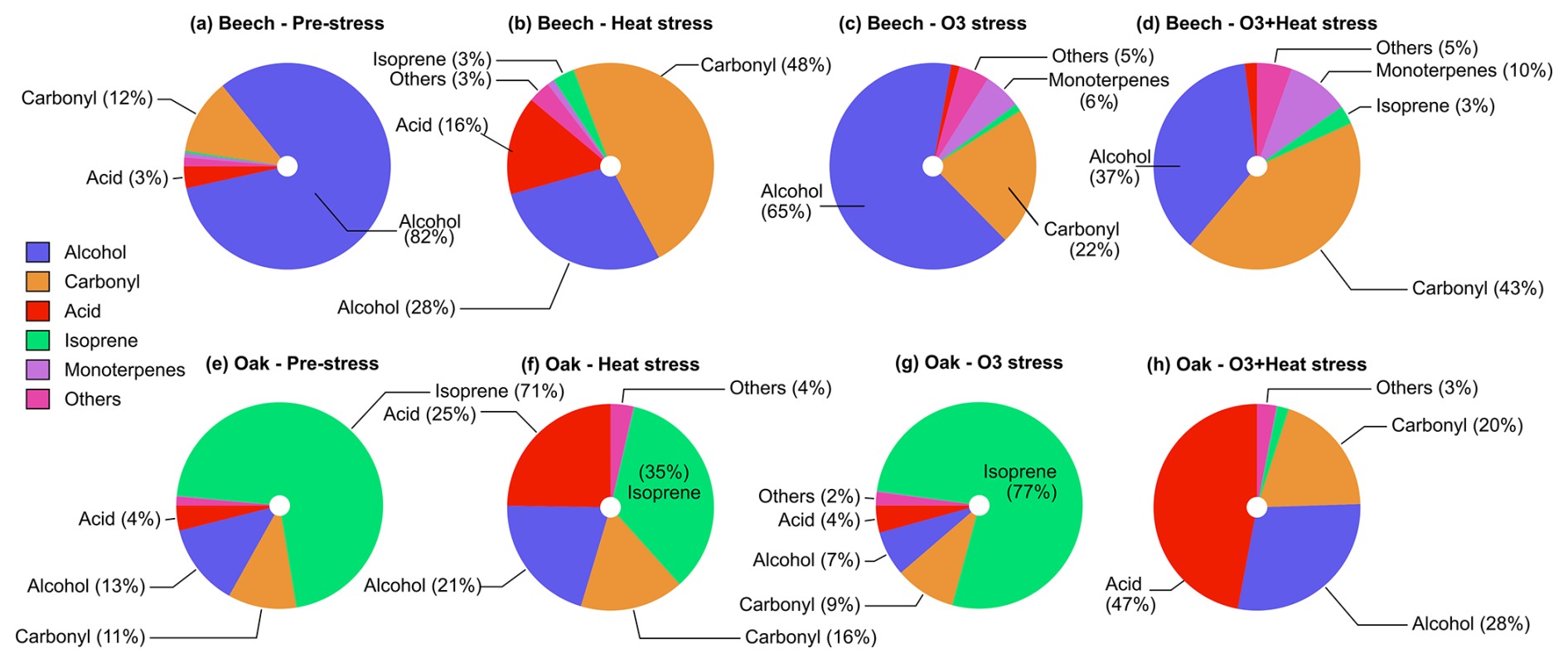
Figure 4 Composition (mole-based) of volatile organic compound classes emitted by (a–d) beech and (e–h) oak under different environmental stress conditions.

Heat stress and combined O₃ + heat stress in beech induced emissions with a more diverse emission profile compared to O₃ and pre-stress stress. The emission profile was dominated by alcohols and carbonyls, which together accounted for over 70 % of the total emissions and monoterpenes (10 %) (mole-based). Among the alcohols, methanol (CH₅O⁺, $m/z$ 33.03), and ethanol (C₂H₇O⁺, $m/z$ 47.05) were the primary contributors, while acetaldehyde, and butanal/methyl ethyl ketone (MEK, C₄H₉O⁺, $m/z$ 73.06) were the main carbonyls. Monoterpenes (10 %) increased substantially under combined stress in beech. Oak emissions were consistently dominated by isoprene pre-stress (71 %), as well as under O₃ (77 %), while contributions from alcohols, carbonyls and acids increased substantially under heat and combined stress. In oak, acetic (C₂H₅O${}_{\mathrm{2}}^{+}$, $m/z$ 61.02) and propanoic acids (C₃H₇O${}_{\mathrm{2}}^{+}$, $m/z$ 75.04) were the main contributor species of the acid fraction. Carbonyl and alcohol composition similar to that of beech. Both species diversified their emitted BVOC mixture under heat and combined stress compared to pre-stress conditions.

OH reactivity was much higher under heat stress rather than combined ozone and heat stress in both species with different magnitudes. Isoprene dominated OH reactivity emitted from oaks under pre-stress and O₃ stress but not heat and combined stress. In beech, heat stress led to OH reactivity dominated by carbonyls (∼ 25 %, mainly acetaldehyde), acids (∼ 27 %, primarily acetic acid), and alcohols (∼ 20 %, mostly methanol), with isoprene (∼ 12 %). When ozone was added on top of heat as a co-stressor, the profile was altered, carbonyls increased to ∼ 30 % (now including more acetone), alcohols remained stable (∼ 20 %), and with more monoterpenes (∼ 20 %) contributions. However, oak showed a different pattern: under heat stress, OH reactivity was driven mainly by isoprene (∼ 56 %) and acids (∼ 23 %, acetic acid). With combined additive (ozone-heat) stress, there was a shift towards the acid group ∼ 66 % and carbonyls to ∼ 14 % (notably hexenal and acetaldehyde), while isoprene dropped to just ∼ 4 %.

In beech, MTs contributed only 1.7 % to emitted OH reactivity under heat stress but ∼ 21 % under combined ozone-heat stress. Oak maintained a minimal MTs-OH reactivity contribution (∼ 1 %) under both heat and combined stress. Monoterpene composition influenced the monoterpene impacts on OH reactivity (Fig. S3). For example, under heat stress, the MT composition in oak emissions changed from the highest contributor being α-pinene (cyclic) towards a higher contribution of more highly reactive citral (acyclic). In beech, sabinene dominated the monoterpene emissions and reactivity during all parts of the experiment, except during heat stress, when the monoterpene composition diversified and emissions of other highly reactive monoterpenes like phellandrene, citral and limonene increased (Fig. S3). The shift towards more acyclic terpenes under stress is in line with other studies (Graham et al., 2024; Khalaj et al., 2021).

O₃ stress substantially reduced total BVOC emissions in both beech (∼ 700 %) and oak (∼ 23 %) compared to pre-stress levels, resulting in a corresponding drop in total OH reactivity by ∼ 200 % in beech and ∼ 7 % in oak (Fig. 5). Interestingly, in beech, O₃-stress phase OH reactivity became dominated by terpenoids (MTs, SQTs), ∼ 25 % of total reactivity, compared to just ∼ 10 % during the pre-stress phase. Oak maintained a consistently isoprene-dominated OH reactivity profile (∼ 90 %) in both stress phases. Physiologically, O₃ alters stomatal regulations and oxidative damage to leaf tissues (more in Sect. 3.2), reducing BVOC biosynthesis and de novo emissions. These emission discrepancies between the species under the same stress also carry the species-dependent stress-action message. While beech appears to shift toward a plastid-centric investment in diverse terpenoid defenses, oak maintains a sustained isoprene production. Moreover, SQT emissions during O₃ stress showed the highest fraction of caryophyllene (Fig. S4), which is among the most reactive sesquiterpenes towards ozone, which could be a potential strategy for protection against oxidative stress.

Although our experiments showed species-specific differences in OH reactivity of BVOC emissions under different stress conditions, one consistent pattern appeared: heat stress consistently elevated atmospheric OH reactivity. This potentially reduces the availability of atmospheric oxidants for other trace gases and can slow down the breakdown of key pollutants (e.g., methane, CO). During heatwaves, elevated VOC emissions combined with high OH reactivity can significantly contribute to the formation of tropospheric ozone (depending on NO_x concentration) and secondary organic aerosols. This effect will be more pronounced in urban and semi-urban areas, where biogenic and anthropogenic emissions interact, especially under intense sunlight.

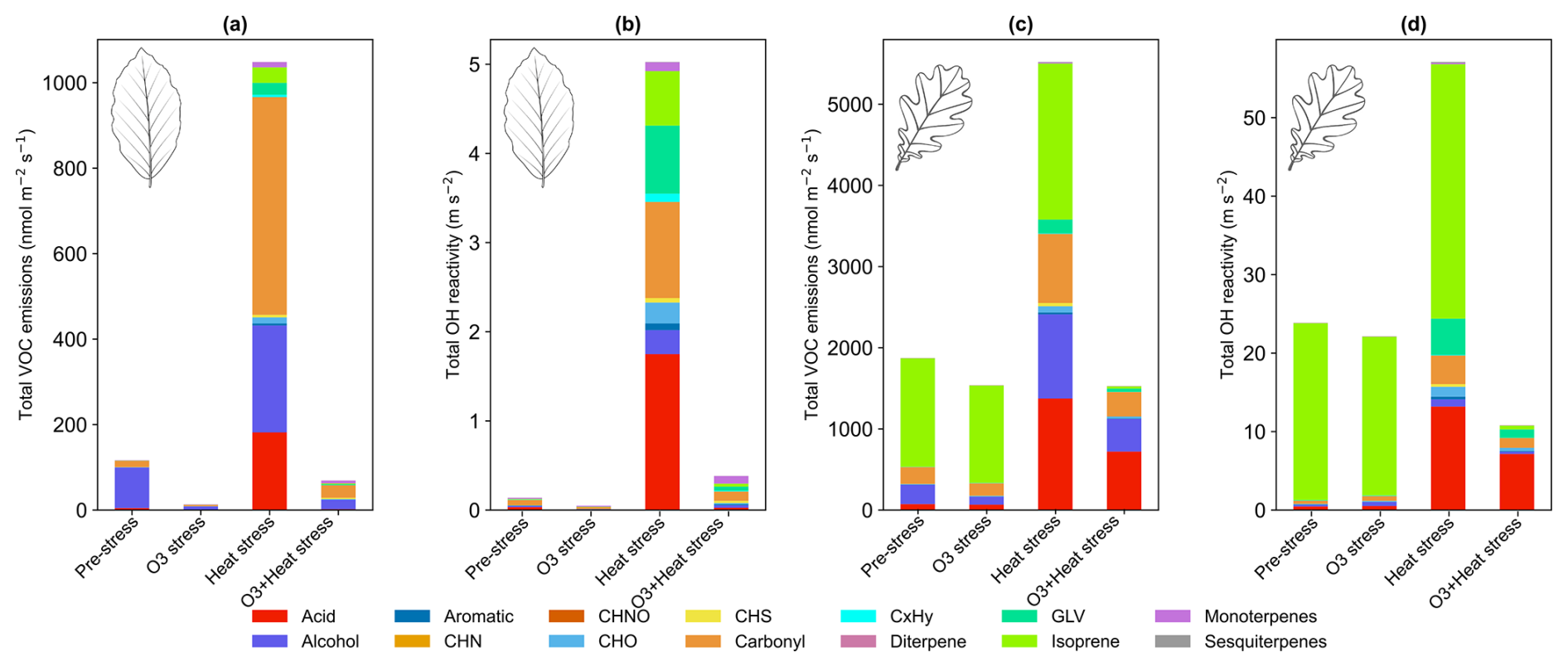
Figure 5 Total volatile organic compound emissions under different stress conditions and their corresponding calculated OH reactivity contributions for (a, b) beech and (c, d) oak.

Comparing with field studies, Churkina et al. (2017) showed that biogenic VOCs contributed ∼ 60 % to ozone formation during the 2006 Berlin heatwave. Additionally, Zhu et al. (2024) showed that the combination of terpenoids and NOx accounted for more than 55 % of the maximum daily 8 h average ozone formation in Los Angeles. Air quality simulations over Paris during June–July 2022 reported urban tree emissions increased secondary organic matter by an average of 5 % (up to 14 % during heatwaves) and ozone concentrations by 1 % on average (up to 2.4 % during heatwaves), with localized increases (Maison et al., 2024). Oak and beech are common tree species found in central and northern European urban and peri-urban areas (Jandl et al., 2025). Our observations, showing that OH reactivity of emissions under heat stress conditions increases by ∼ 97 % (beech) or ∼ 58 % (oak), support the expectation that ozone pollution in urban areas may increase with more frequent heat waves.

In the real world, especially in an urban atmosphere, several stressors occur at the same time, so that a discussion of additive stress is important. Based on our experiment, beech trees increase their OH reactivity of emissions by ∼ 60 % under combined ozone and heat stress, whereas oaks reduce it by ∼ 54 %. In the context of European cities and forests, this becomes especially important. Central and Western Europe, including countries like Germany, has large areas dominated by European beech (e.g., in Germany 14.8 %), which may lead to increased atmospheric oxidation potential. Naturally, with species heterogeneity in forests, compensatory effects are possible: one species may increase while another decreases OH reactivity, and OH reactivity may be not change substantially overall. A critical concern is the physiological consequences of prolonged additive stress, as evidenced by our experiment, where all plants wilted and died by the end of the combined stress period. Beyond atmospheric consequences, additive stress poses a potential threat to tree vitality and forest ecosystem resilience.

3.4 Random forest model

3.4.1 Consistency and uncertainties

The classification matrix for all classes from the trained random forest model for beech and oak shows precision and recall of 0.95 to 1.0 (Figs. 6a–b). It compares predicted versus actual stress categories, where the diagonal elements represent correct predictions (true positives) and off-diagonal elements indicate misclassifications. Precision reflects how many samples predicted for a class were correct, recall measures how many true samples of that class were correctly identified, and the F₁-score combines both into a balanced accuracy measure. From the matrix, it is clear that the model can effectively discriminate between the different stresses.

Model evaluation was not restricted to standard classification metrics but was extended to explore the classification's consistency, reliability, and uncertainty. Shannon Entropy (uncertainty in prediction) was used to quantify the classification confidence (Fig. 6c–d). Entropy values close to 0 indicate that the model made confident predictions (i.e., one class strongly dominated the probability distribution), whereas higher entropy values reflect greater uncertainty between classes. Most samples showed low entropy values, indicating that the classifier was highly confident across most conditions. A smaller number of predictions have moderate to high entropy (but less than the threshold).

To further assess the relationship between uncertainty and misclassification, entropy distributions were compared between correctly and incorrectly classified samples (Fig. 6e–f). Incorrect predictions were generally associated with comparatively high entropy, confirming that the entropy well captured classification uncertainty rather than random variability. Also, no random entropy spikes were observed across conditions, supporting the model's stability. In addition, the time series entropy (see Figs. S5d and S6d) showed that most classifications were made with high certainty (entropy < 0.6), though slight increases occurred under combined O₃ + heat stress, potentially reflecting overlapping BVOC patterns and the model's sensitivity to complex stress signals. Performance stability was also checked across classes; bootstrapped distributions of classification scores with low variance (Figs. S5e–f, S6e–f) indicate the model's consistency. These evaluations confirmed that trained models are useful in classifying stress types.

The UpSet plots (Figs. 6g–h) show the dominant BVOC fingerprints (SHAP-derived compounds) that contributed most strongly to classifying each stress type and shared or overlapping compounds between stresses. For example, certain VOC features appeared across both O₃ and combined O₃ + heat stress, suggesting common biochemical pathways or coordinated defense mechanisms.

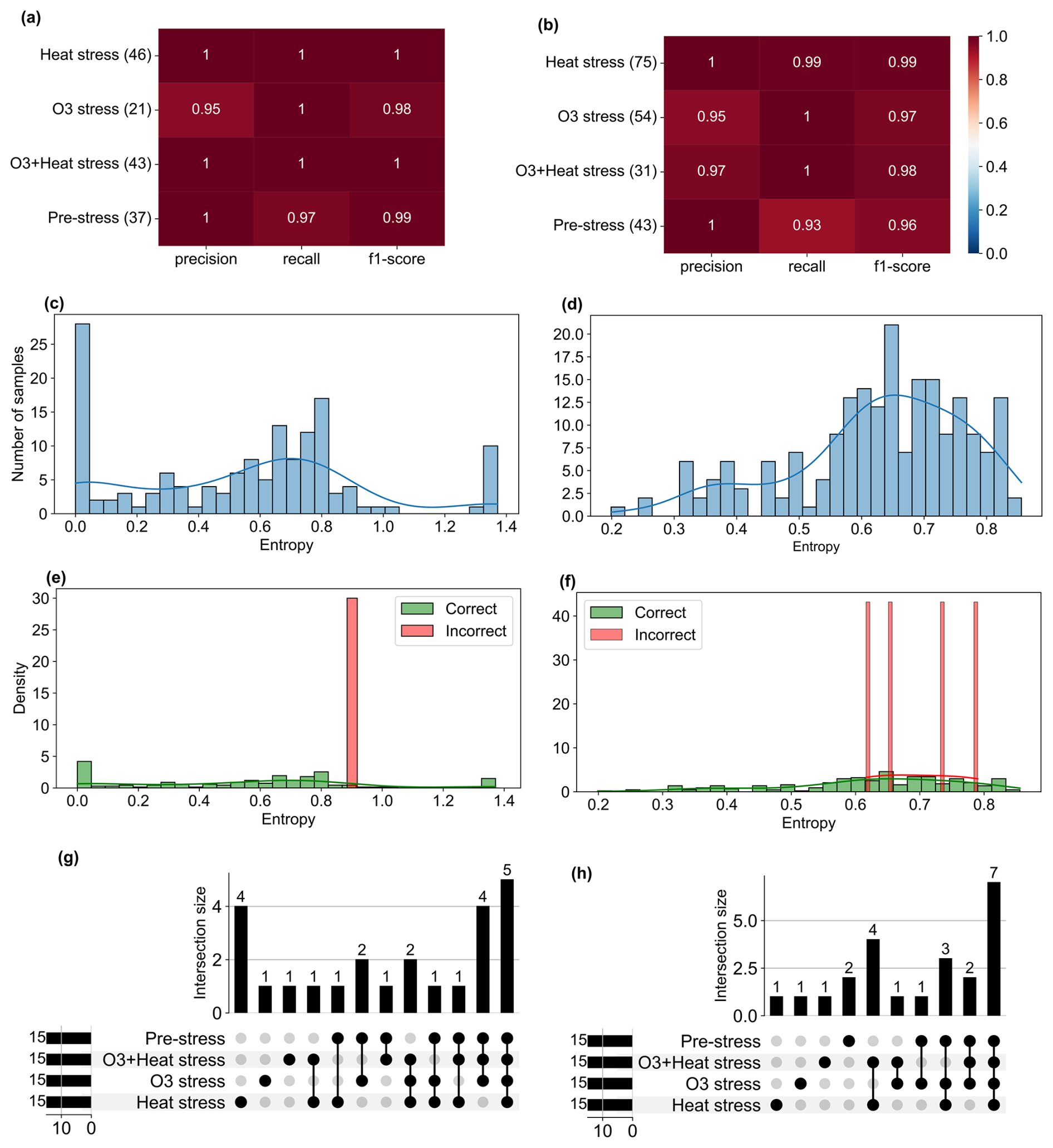
Figure 6 Performance metrics, uncertainty, and misclassification analysis of the Random Forest model for stress classification in (left) beech and (right) oak. (a–b) Precision, recall, and F₁-score for each stress class based on the test set. Numbers in parentheses indicate the number of test samples per class. (c–d) Distribution of Shannon entropy values of predicted class probabilities across all test samples. (e–f) Entropy distributions of correctly and incorrectly classified samples. (g–h) Plots showing intersections of SHAP-identified top 15 stress markers among the four stress classes. Bars represent the number of ions unique to or shared between classes. Insets indicate total counts.

3.4.2 SHAP resolved stress fingerprints

SHAP values from Random Forest models (Figs. A1 and A2 in the Appendix A) were used to identify stress-specific compound fingerprints for both beech and oak, as well as interspecific differences associated with stress conditions. Beech primarily depended on a limited number of compounds under each stress scenario (Fig. 7a). In the O₃ stress condition, markers such as propanol (C₃H₉O⁺, $m/z$ 61.06), methanol (CH₅O⁺, $m/z$ 33.03), ionone (C₁₃H₂₁O⁺, $m/z$ 193.15), and tolualdehyde (C₈H₉O⁺, 121.06) were most prominent, typically contributing with positive SHAP values when suppressed or low emission rate (Figs. 7a and A1). These patterns point toward ozone-induced suppression of certain biosynthetic pathways (details Sect. 3.2). Under heat stress, the most dominant contributors included C5 carbonyls (C₅H₁₀O⁺, $m/z$ 87.08), methyl-vinyl-ketone (MVK, C₄H₇O⁺, $m/z$ 71.05), phenethyl acetate (C₁₀H₁₃O${}_{\mathrm{2}}^{+}$, $m/z$ 165.01), isoprene, benzoid fragments (C₆H${}_{\mathrm{7}}^{+}$, $m/z$ 79.05, possibly from shikimate pathway products), hexanal (C₆H₁₃O⁺,$m/z$ 101.09) and cumenol (C₉H₁₂OH⁺, $m/z$ 137.09). Their increased emissions significantly shifted predictions towards the heat stress class. These BVOCs reflect thermal degradation and markers of heat stress. Interestingly, under combined O₃ + heat stress, monoterpenes (C₁₀H${}_{\mathrm{17}}^{+}$, $m/z$ 137.13) were strongly activated (Fig. 3a) and have high positive SHAP values (Figs. 7 and A1d), forming a unique and dominant fingerprint for beech under O₃ + heat stress.

Similar to beech, under nighttime ozone stress, oak showed several BVOCs such as propanol, acetaldehyde, sesquiterpenes and pyruvic acid were identified with high SHAP values, despite their low absolute intensities in ozone-stressed samples. The classifier assigned strong predictive importance to their reduced presence, meaning lower emissions (Table S4) of these features were informative for ozone-related stress discrimination. Such low-emission driven feature patterns highlight that the model's decision was not driven by elevated emissions but rather by reducing specific volatiles during ozone exposure. Oak's heat stress fingerprints were primarily shaped by elevated pyruvic acid (C₃H₅O${}_{\mathrm{3}}^{+}$, $m/z$ 89.02), formic acid (CH₃O${}_{\mathrm{2}}^{+}$, $m/z$ 47.01), tolualdehyde, isoprene, and phenol (C₆H₇O⁺, $m/z$ 95.05) emissions (Fig. 7b). The combined O₃ + heat stress condition showed a compound profile largely driven by markers shared with the individual stress states, but with amplified effect sizes. Particularly, sesquiterpenes, MVK, phenethyl acetate (C₁₀H₁₃O${}_{\mathrm{2}}^{+}$, $m/z$ 165.09), benzoid fragments, formic acid, and ionone were dominant BVOC fingerprints.

A limited number of BVOC (20 %–25 % of the total emission signal) were unique to individual stress conditions among the top 15 stress fingerprint compounds in both species. Several BVOCs consistently appeared as markers for specific stress types, independent of species, while others showed species-specific stress. These overlapping BVOC fingerprints or signatures imply that certain VOCs may reflect core metabolic responses to abiotic stress, regardless of species-specific physiology.

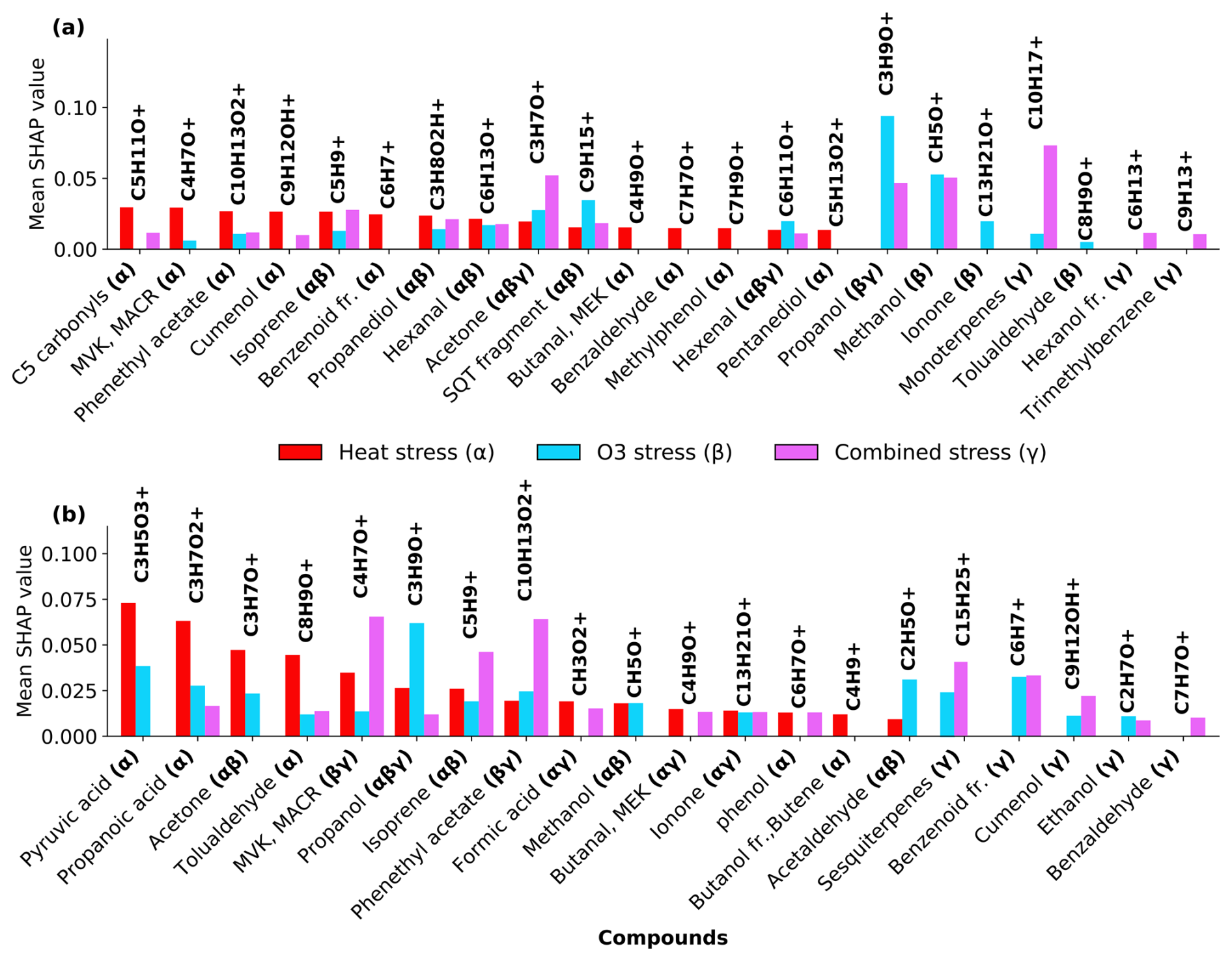
Figure 7 SHAP-based (SHapley Additive exPlanations) feature importance of volatile organic compounds (VOCs) for classifying stress conditions in beech (a) and oak (b). “fr.” refers to fragments. Bar plots show the mean SHAP values of potential VOCs fingerprint under heat stress (α), ozone stress (nighttime) (β), and combined O₃ + heat stress (γ).

3.5 Positive matrix factorization

3.5.1 PMF factor interpretation

PMF was used to apportion the stress profile and identified a six-factor solution for both beech (Fig. 8) and oak (Fig. 9). Details about the PMF analysis and the rationale for selecting the six factors are provided in Sect. 2.2.2 and Appendix B.

In Beech, Factor 1 is characterised as the “Pre-stress or baseline factor” because it shows consistent and low signal intensity throughout the period (Fig. 8). Additionally, it has weak correlations between the top contributing VOCs and with the factor-time series, and the explained variance for these compounds was minimal. This reflects the background emissions under unstressed conditions. Factor 2 is termed the “late heat response” factor due to its steady emissions increase (after ∼ 38 °C) beginning toward the end of the O₃ + heat phase and continuing into the heat stress period. This gradual rise coincides with the sharp increase in chamber temperature, indicating that this factor likely captures delayed thermal stress responses. Factor 3 is identified as the “plant decay” factor, as it becomes prominent after the stress, and the time series suggests a delayed emission peak independent of immediate heat or ozone exposure. This temporal dissociation implies involvement in cell lysis, consistent with the observation that all plants had wilted by the end of the experiment. Factor 4 is considered the “combined stress” factor, as it shows a distinct peak coinciding with the period of simultaneous O₃ + heat exposure. The time series shows a rapid, stress-synchronous response. Factor 5 is designated the “severe heat stress” factor, characterized by a sharp and isolated peak during the highest temperature phase of the experiment (42 °C), without overlap from ozone exposure. Factor 6 is interpreted as the “early heat stress” factor, with a narrower temporal window earlier than the main O₃ + heat peak and displays an earlier response to rising temperatures (∼ 36–38 °C) before full stress onset.

In Oak, Factor 1 is identified as the “Pre-stress or baseline factor” due to its moderate contribution across all phases, including the pre-stress and early ozone exposure, without showing any substantial sharp peak (Fig. 9). Its VOC composition is broad but with low correlation (without considering isoprene, oak generally emits isoprene) and explained variance for most top compounds, likely representing constitutive emissions and ambient-level biological activity. Factor 2 is associated with the “O₃ + heat stress,” peaking sharply during the overlapping ozone and heat phase. Factor 3 is labelled the “late heat stress factor,” as it indicates a delayed increase after the peak heat stress events have abated. Factor 4, termed the “initial heat stress factor,” dominates during the standalone heat phase and peaks just after the onset of heat stress. Factors 5 and 6 are described as the “severe heat stress,” showing the maximum contribution during the peak heat stress temperature (∼ 42 °C), after which they consistently decline.

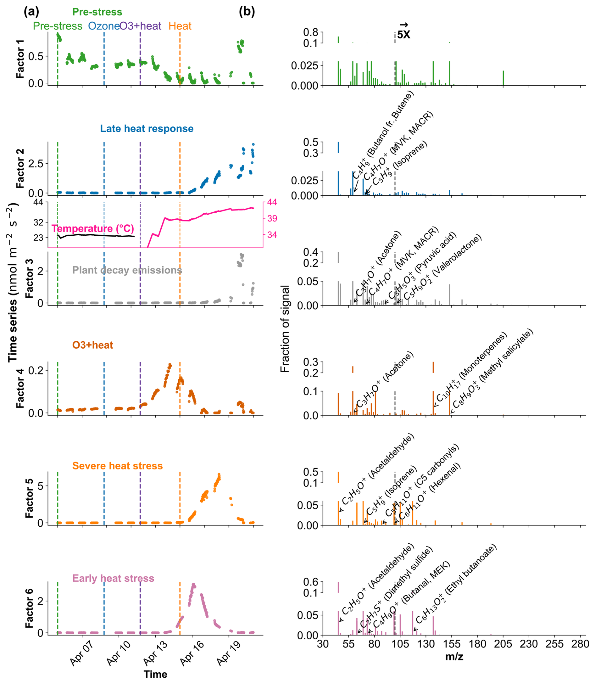
Figure 8 Positive Matrix Factorization (PMF) analysis of VOC emission profiles from beech under different environmental stress conditions. (a) Time series of a six-factor PMF solution. Colored vertical dashed lines indicate the starting of different stress phases. (b) Corresponding mass spectra ($m/z$ profiles) of each factor and their relative signal contributions, $m/z$ 100–280 are scaled by a factor of 5.

3.5.2 PMF-resolved stress-VOCs profiles for stress fingerprints

The early heat stress factor for beech (Fig. 10a) was characterized by hexenal, isoprene, ethyl butanoate (C₆H₁₃O${}_{\mathrm{2}}^{+}$, $m/z$ 117.09), MEK, and monoterpene fragments (C₆H${}_{\mathrm{9}}^{+}$, $m/z$ 81.07). Similar fingerprint patterns were also seen in the severe heat stress and late heat response factors. Additionally, the severe heat stress factor uniquely showed contributions from MVK, benzenoid fragments, and C₅H₈O (C₅H₈OH⁺, $m/z$ 85.06), making it apart from the other heat-related factors. These findings are consistent with studies showing that temporary heat stress triggers the biosynthesis of GLVs (e.g, hexenal) and isoprene, which serve as rapid markers of membrane perturbation and ROS signaling within leaf tissues (Bao et al., 2023; Kleist et al., 2012; Turan et al., 2019). Particularly, isoprene is well-documented to increase cell membrane stability during thermal stress and is frequently emitted by deciduous trees under elevated temperatures (Bao et al., 2023; Iwasa et al., 2024). As heat stress persists, the VOC emission for late heat stress remains similar but becomes more complex with contributions from MVK, benzenoid fragments, and C₅H₈O (C₅H₈OH⁺, $m/z$ 85.06). MVK emissions are predominantly endogenous under thermal stress (Cappellin et al., 2019), and benzenoid compounds accumulate during acute heat exposure (Liu et al., 2022b), representing the activation of distinct stress-related metabolic shifts over time.

The O₃ + heat stress factor showed (Fig. 10 a) a distinct VOC response and was strongly dominated by monoterpenes (C₁₀H${}_{\mathrm{17}}^{+}$, $m/z$ 137) with additional supporting signals from monoterpene fragments, acetone (C₃H₇O⁺, $m/z$ 59.04), Methyl salicylate (C₈H₉O${}_{\mathrm{3}}^{+}$, $m/z$ 153.05) and propendiol (C₃H₈O₂H⁺, $m/z$ 77.05). Elevated monoterpene emissions are generally attributed to temperature-induced responses in plants and have even been described as a 'thermometer of plants' (Jardine et al., 2017). Furthermore, monoterpenes serve as antioxidants, helping to mitigate oxidative stress caused by both elevated temperatures and ozone by quenching ROS and contributing to cross-tolerance against double abiotic stresses. On the other hand, acetone emissions have been associated with cellular decay and ozone-induced damage, as described in several studies (Davison et al., 2008; Loubet et al., 2022; Wu et al., 2019).

The plant decay factor was temporally shifted toward the end of the experiment, particularly after the peak of combined O₃ + heat stress. The chemical profile was not distinct from the other factors, with typical stress marker compounds, e.g., acetaldehyde, ethanol, acetone, hexanal, benzoid fragments, and isoprene. Most of these low $m/z$ compounds, notably ethanol, acetone, and acetaldehyde, are by-products of altered respiratory activity and fermentative metabolism under high temperature as discussed before, may be due to cell-lysis.

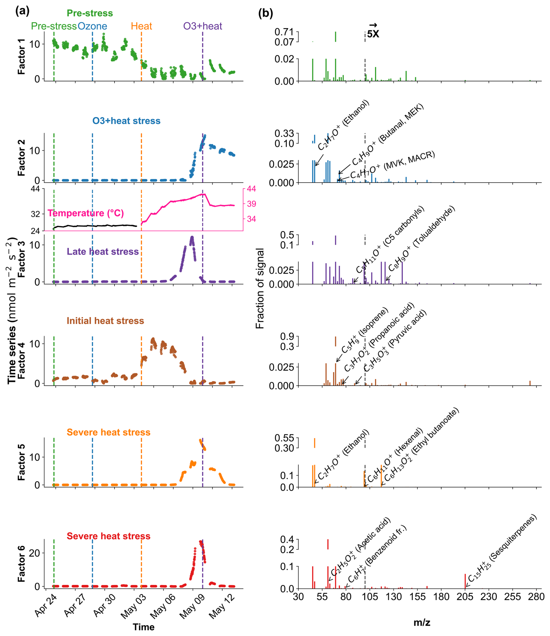
Figure 9 Positive Matrix Factorization (PMF) analysis of VOC profiles in oak under different environmental stress conditions. (a) Time series of a six-factor PMF solution. Colored vertical dashed lines indicate the starting of different stress phases. (b) Corresponding mass spectra ($m/z$ profiles) of each factor and their relative signal contributions, $m/z$ 100–280 are scaled by a factor of 5.

In oak (Fig. 10b), initial heat stress was characterized by distinct fingerprints of isoprene, propanoic acid, MEK, pyruvic acid (C₃H₄O${}_{\mathrm{3}}^{+}$, $m/z$ 87), and cyclopentadiene. Interestingly, a similar VOC signature reappeared during the late heat stress phase, and this recurrence suggests that both the duration and intensity of thermal exposure led to repeated cycles of oxidative metabolism and membrane adjustment. Elevated isoprene is a hallmark VOC in oaks and responds sharply (Table S4) to rapid temperature increases as thermoprotectant (Li et al., 2010). Also, the co-presence of pyruvic acid, MEK, and propanoic acid could be due to activated glycolytic and pyruvate turnover pathways to supply energy for thermal resilience (Loreto and Schnitzler, 2010). In contrast, severe heat stress induced a distinct chemical signature dominated by sesquiterpenes, benzenoid fragments, hexanal, and ethyl butanoate. These compounds are often linked to more advanced or prolonged heat stress responses as discussed earlier in beech, potentially involving membrane degradation and lipid oxidation.

The factor associated with the combined O₃ + heat stress showed (Fig. 10b) unique dominance of acetone, acetic acid, MVK, MEK, butene, and ethanol. Acetone has been associated with cellular decay and ozone damage in multiple studies (Davison et al., 2008; Loubet et al., 2022; Wu et al., 2019). Notably, the co-emission of MVK and MEK supports the mechanistic model by Cappellin et al. (2019), which showed that MEK could be produced biogenically from MVK within plant tissues via stress-induced pathways decoupled from isoprene biosynthesis. The presence of MVK and MEK in high abundance (Table S4) under combined O₃ + heat stress, but not necessarily under isolated ozone or heat periods, emphasizes that this transformation pathway is particularly prominent when plants simultaneously encounter intensified ozone and heat stress.

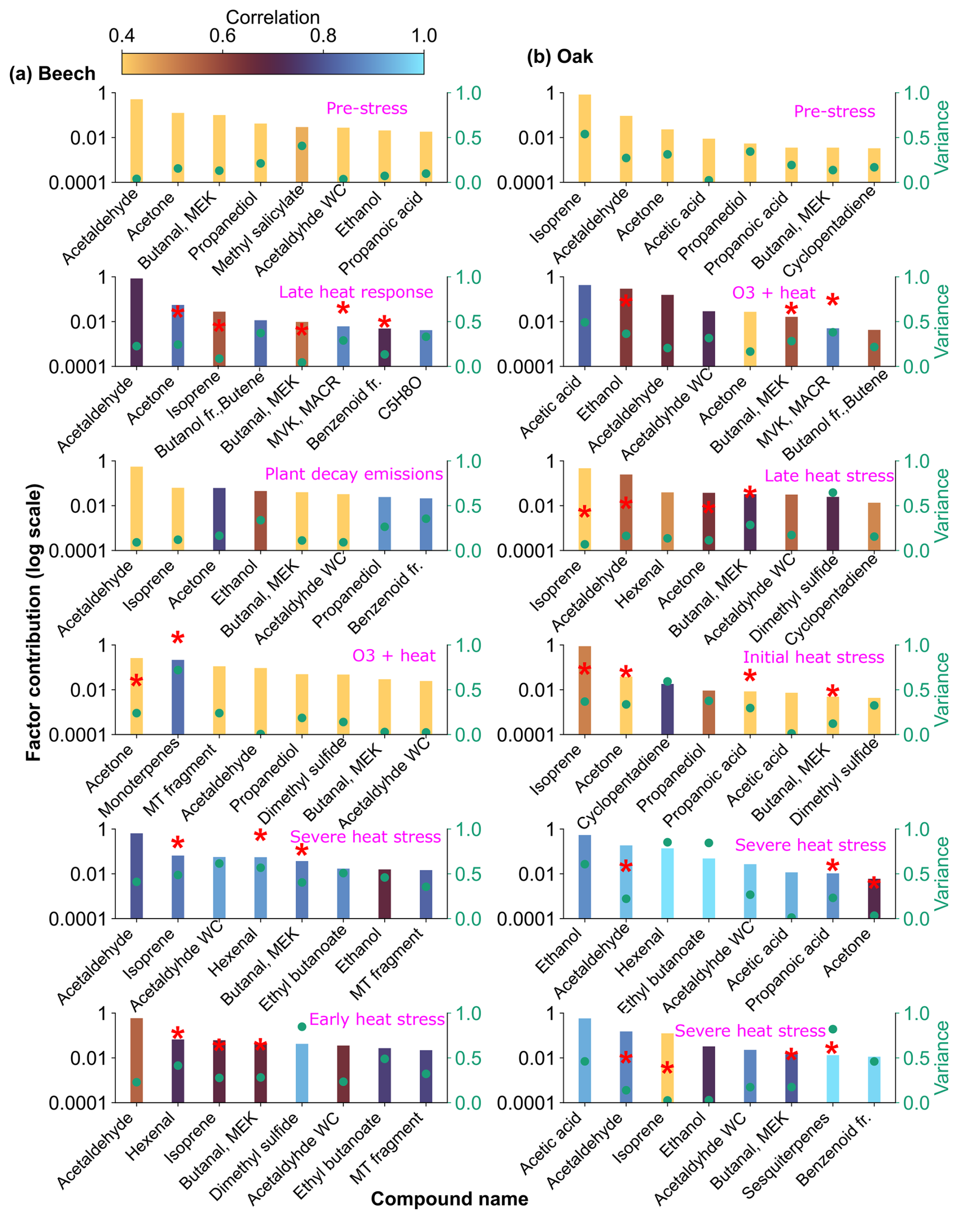
Figure 10 Top 8 stress-BVOC markers for each factor for (a) Beech and (b) Oak. Bar plots show the relative contribution of specific compounds, while green dots represent the correlation coefficient with the respective factor time series. Color shading indicates their correlation with the corresponding factor timeseries, and asterisks (*) denote compounds that were also identified as fingerprints by the machine learning.

3.6 Do ML and PMF tell the same story of stress-specific fingerprints?

Both PMF and ML approaches identified overlapping VOC fingerprints for specific stressors, along with species-specific differences in these fingerprints (Table 2). For example, elevated isoprene appeared as a heat stress marker across both species, signifying it could be a potential universal heat stress marker. Conversely, elevated sesquiterpenes were found as markers only for severe heat stress for oak, which may be related to the non-generalizable sesquiterpene emissions we induced in the beech experiment by having to cut one branch. Stress-BVOCs like acetone, MVK, MEK, and benzenoid fragments, although marked in both species, varied in intensity and timing, showing possible differences in oxidative stress responses or cell membrane degradation (Fig. 10).

Table 2 Stress-specific volatile organic compound fingerprints in Beech and Oak under heat, ozone, and combined ozone + heat stress. Superscripts denote identification by Machine Learning (ψ) or Positive Matrix Factorization (φ).

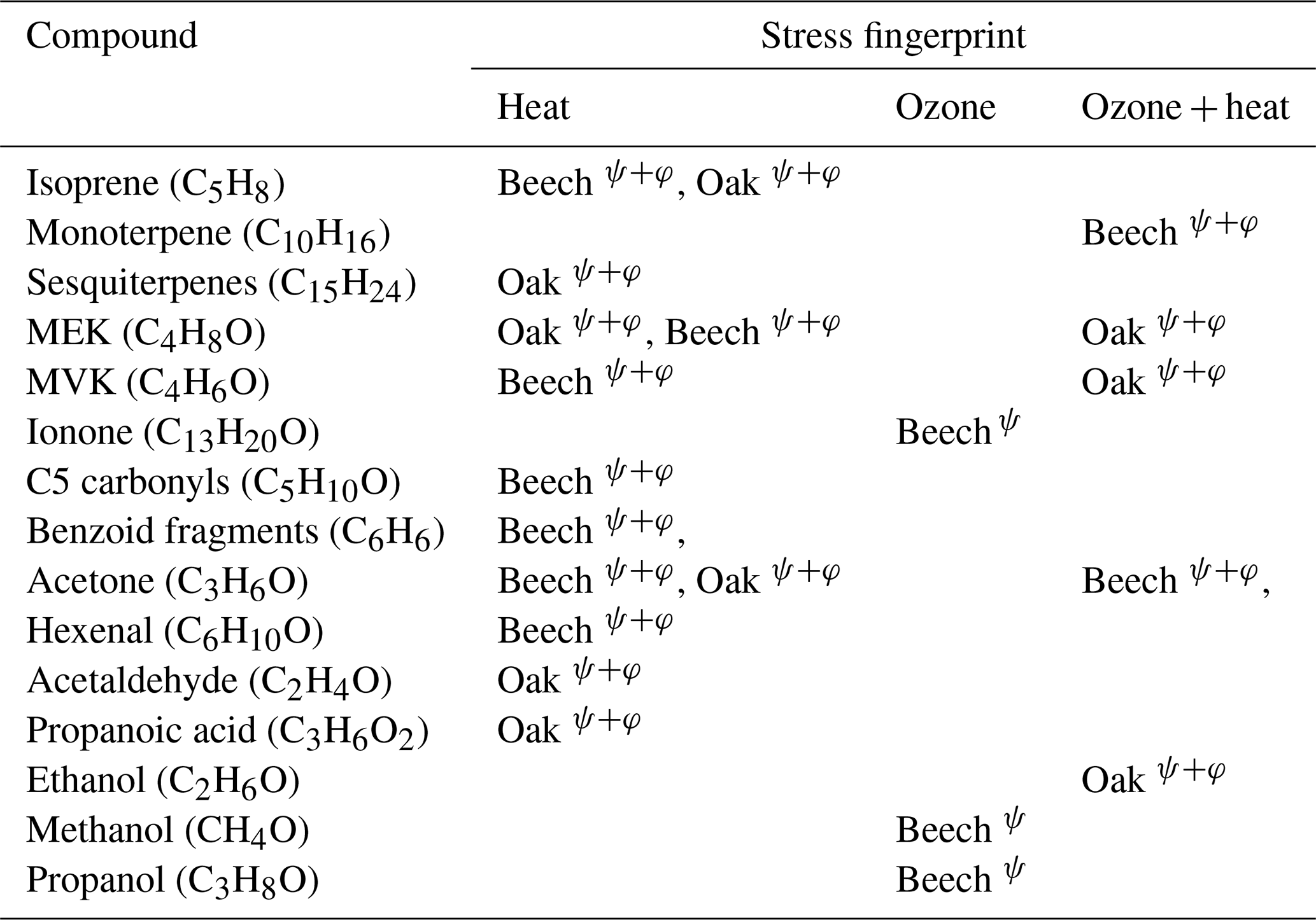
PMF, being an unsupervised approach, identifies hidden factors based on variance structures within the data, whereas ML classification is a supervised method guided by predefined stress labels. Consequently, while both approaches converged on the same dominant fingerprints, the ML model identified several additional ozone-specific markers that PMF did not resolve, potentially because of their small magnitude. Conversely, PMF successfully differentiated contextual emission patterns (e.g., early, late heat stress) (Figs. 8–9). The additional rationale for using these fundamentally different approaches was to evaluate how consistently they capture stress-related features and how effectively they can distinguish overlapping stress events. As shown in Table 2, a substantial proportion of the identified fingerprints were consistent between both methods. Collectively, PMF and ML offer complementary perspectives: PMF elucidates temporal emission patterns, whereas ML identifies the most informative features for distinguishing stress types.

3.7 Consequences of a shift to stress-related biogenic VOC emission patterns in a warming climate

Projected climate change trends indicate an increase in the frequency of hot days and heatwaves, leading to compound heat-ozone waves (Hertig et al., 2020; Yang et al., 2022). The relative contributions of various BVOC classes emitted by beech and oak trees are expected to shift significantly due to heat stress (Fig. 7). Thus, urban areas containing such trees may experience a notable alteration in the composition of emitted BVOCs, with biogenic sources becoming increasingly influential on urban air quality. For instance, elevated isoprene and monoterpene emissions during heat stress can enhance ozone formation potential, as these compounds readily react with atmospheric oxidants, thereby raising ozone levels in urban environments where high levels of nitrogen oxides from combustion are present, particularly on hot summer days (Pfannerstill et al., 2024).

Moreover, O₃ itself reacts with olefinic BVOCs like isoprene and terpenes to produce additional OH radicals (Di Carlo et al., 2004), creating a positive feedback loop that can amplify BVOC oxidation in the atmosphere. This OH production from O₃-BVOC reactions can further extend tropospheric ozone and secondary organic aerosol formation, compounding the effects of heatwaves on urban pollution levels. Also, the rising prevalence of BVOCs under warmer conditions raises concerns regarding their interactions with anthropogenic emissions. In areas with both high nitrogen oxide levels and high BVOC emissions from vegetation, this loop could drive periodic spikes in ozone and fine particulate matter, contributing to regional pollution events.

4 Conclusion

This study provides an investigation of how biogenic volatile organic compounds (BVOCs) are modulated in response to heat and nighttime ozone stress, by two dominant deciduous European forest tree species, beech and oak, and to our knowledge, for the first time, in response to the combination of both stressors. Our findings highlight distinct species-specific patterns in the emissions of key BVOCs like isoprene, monoterpenes, sesquiterpenes, and green leaf volatiles, which vary considerably depending on the type of stress encountered. Combined ozone + heat stress elicited emission responses that were distinct from both singular stress applications, highlighting the complexity of real-world stress scenarios where multiple stressors likely happen in combination. In order to facilitate stress identification in future field measurements, we identified stress-specific fingerprint BVOC markers for each stress using machine learning (Random Forest) and cross-validation by Positive matrix factorization (PMF).

Beech switched from a low/non-isoprene emitter to an isoprene emitter under heat stress. While oxidative stress (∼ 120 ppb O₃) suppressed the isoprene emissions by 16 %, the addition of heat still led to a considerable increase, though less than heat alone. Though Oak is a high isoprene emitter, its isoprene emissions were reduced under stress. Under combined ozone + heat stress, they decreased significantly. Green leaf volatiles were substantially increased by heat stress and less by combined stress in both species, while ozone stress barely affected the green leaf volatiles. Beech activated plastid-localized pathways under heat and combined ozone + heat stress, whereas oak relied on cytosolic and membrane-associated defenses. Total molar BVOC emissions decreased under O₃ stress in both species compared to pre-stress, were highest under heat stress, and went back to a similar range as pre-stress under combined O₃ + heat stress. Emitted OH reactivity followed the same pattern, with the highest emitted OH reactivity under heat stress for both species.  Distinct VOC fingerprints were associated with specific stress types in each species. For example, in beech, combined stress was uniquely marked by increased monoterpenes emission. In oak, it was characterized by elevated methyl-vinyl-ketone and ethanol.

As a caveat, the experiment involved branch cutting to fit one beech plant into the plant chamber, which may not fully replicate the acclimation phase of this species properly. The induction of sesquiterpenes through cutting in beech limits the generalizability of some pathway results. Additionally, since stress treatments were applied sequentially and in different orders for the two species, sequence-specific effects cannot be separated from overall stress responses. The outcomes thus represent species-specific responses under the applied sequences rather than generalizable effects of stress order. Since the duration and intensity of stress influence how much it changes plant emissions, our results may not be generalizable for all ozone, heat, and O₃ + heat situations. Future research could validate our findings through integrative approaches (including factorial or randomized stress sequences), on the one hand going into biomolecular directions for a better understanding of the plant reactions, and on the other hand photochemical oxidation of the plant emissions to investigate their impact on atmospheric chemistry. The stress-specific BVOC markers identified in this study proposed an auspicious path for rapid stress detection in Beech and Oak, yet their broader applicability across species (in landscape level) or even within different genotypes of the same species remains an open question.

Our findings demonstrate that tree species under combined abiotic stress can either amplify or reduce their contribution to atmospheric reactivity, depending on species-specific physiology and stress magnitude. This has direct consequences for tropospheric ozone formation, secondary organic aerosol formation, and urban air quality, especially during heat waves. As heatwaves and pollutant stress events become more frequent due to climate change, shifts in VOC emissions and potential dieback in sensitive species like beech could significantly alter atmospheric chemistry, ecosystem function, and carbon budgets. As knowledge on the interactions between multi-stressed trees and the atmosphere grows, these dynamics must be incorporated into regional climate models and policy planning for urban greening and forest management.

Appendix A: SHapley Additive exPlanations: Random Forest

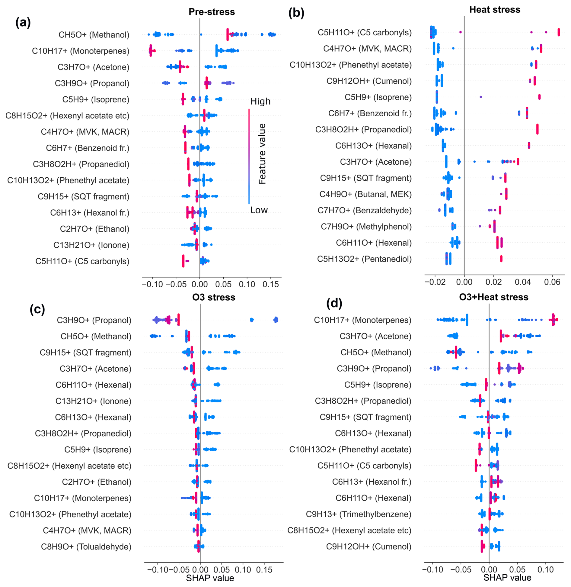
Figure A1 SHAP summary plots based on the trained Beech Random Forest model the top 15 important BVOC features for classifying each stress condition. (a) Pre-stress, (b) heat stress, (c) O₃ stress, and (d) O₃ + heat stress. Each point represents a SHAP value for a specific compound in an individual sample, with colors indicating feature value. Positive SHAP values indicate a stronger association with the predicted stress class.

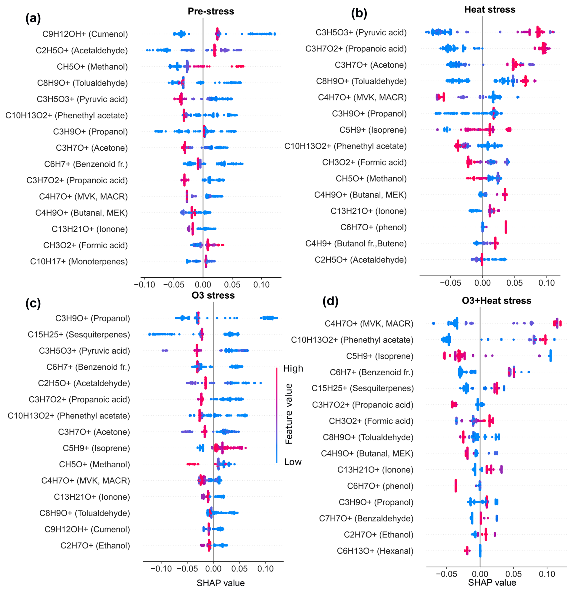
Figure A2 SHAP summary plots based on the trained Oak Random Forest model the top 15 important BVOC features for classifying each stress condition. (a) Pre-stress, (b) heat stress, (c) O₃ stress, and (d) O₃ + heat stress. Each point represents a SHAP value for a specific compound in an individual sample, with colors indicating feature value. Positive SHAP values indicate a stronger association with the predicted stress class.

Appendix B: Positive Matrix Factorization (Validation)

In beech and oak PMF, a range of possible solutions 3 to 10 factors were evaluated through a series of quantitative analysis. The choice of the 3 to 10 factor range was based on the expected complexity of plant VOC emissions, which are influenced by multiple overlapping processes including baseline metabolic activity, temperature-induced emissions, ozone responses, or decay. Solutions with fewer than three factors were excluded from the outset as biologically implausible. Conversely, solutions above 10 factors tended to produce overly fragmented and unstable profiles, making them less reliable for interpretation and comparison. As mentioned in Sect. 2.2.2, multiple checks were performed before deciding on the final solution. One last strategy was to test the PMF factor solution, how each factor reproduces the temporal structure of the raw VOC signals, and the residual (unexplained) signal. All potentially stress-relevant BVOCs (identified through ML) were assessed for reproducibility and residual (unexplained) signal to ensure the selected factor solution is statistically robust.

For example, for beech, the 3 to 5 factor solutions substantially underestimated monoterpene peaks during combined ozone and heat stress phases (Fig. B1a–c). On the other hand, solutions with 7 or more factors began to split monoterpenes into separate profiles, introducing artifacts such as unrelated low-level noise contributions (Fig. B1e). Based on this, the 6-factor solution was selected as it reproduces the peak intensities and temporal patterns without introducing overfitting artefacts or excessive noise (Fig. B2).

Similarly, for oak, sesquiterpenes were poorly captured in lower-factor solutions (Fig. B3). These high-mass compounds were either lumped into broad stress-related profiles or ignored altogether, leading to underrepresentation. Only in the 6-factor solution was a distinct and coherent representation of sesquiterpenes observed in Oak, aligning with stress onset and peak emissions. Beyond the 6 factors, this signal began to fragment.

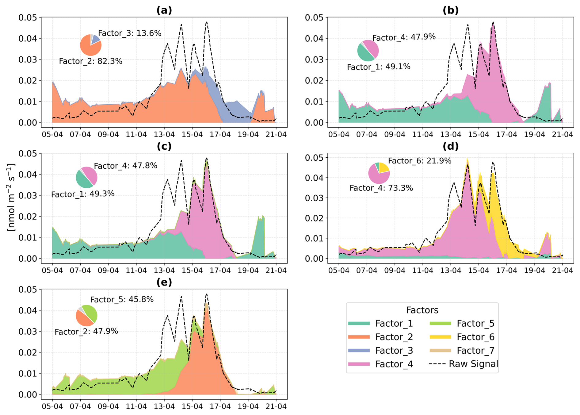
Figure B1 Stacked monoterpene time series showing PMF-resolved factor contributions for 3-factor (a) to 7-factor (e) solutions in Beech. Each subplot represents a different PMF solution. Colored areas correspond to contributions from individual factors, while the white area under the curve indicates unexplained. Inset pie charts represents the total contribution of each factor to the monoterpene signal.

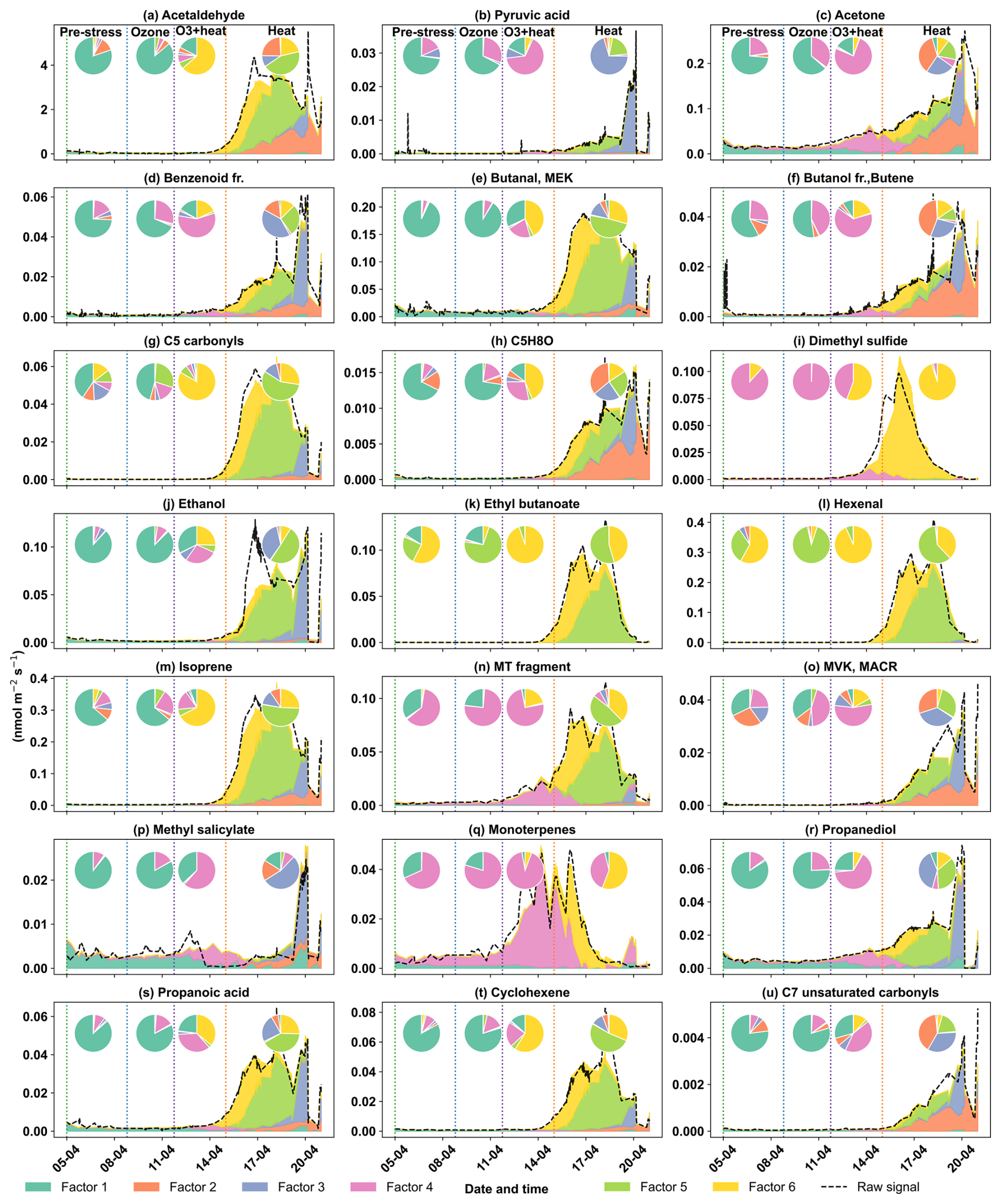
Figure B2 Stacked time series of PMF-resolved contributions for selected BVOC compounds during the Beech experiment. The black dashed lines indicate the original concentration of specific compounds, while stacked colored areas represent contributions from the six PMF-resolved factors. Each compound's emission is displayed across the four stress periods (Pre-stress, O₃ stress, O₃ + Heat stress, Heat stress), separated by vertical dashed lines. Inset pie charts show the relative contribution of each factor to compound emissions within each stress period, as a factor dominance.

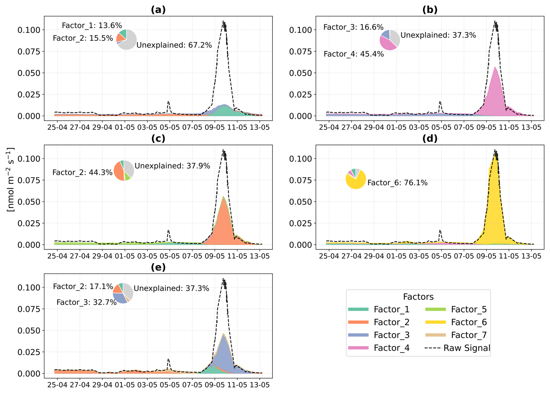
Figure B3 Stacked sesquiterpenes time series showing PMF-resolved factor contributions for 3-factor (a) to 7-factor (e) solutions in Oak. Each subplot represents a different PMF solution. Colored areas correspond to contributions from individual factors, while the white area under the curve indicates unexplained. Inset pie charts represents the total contribution of each factor to the sesquiterpenes signal.

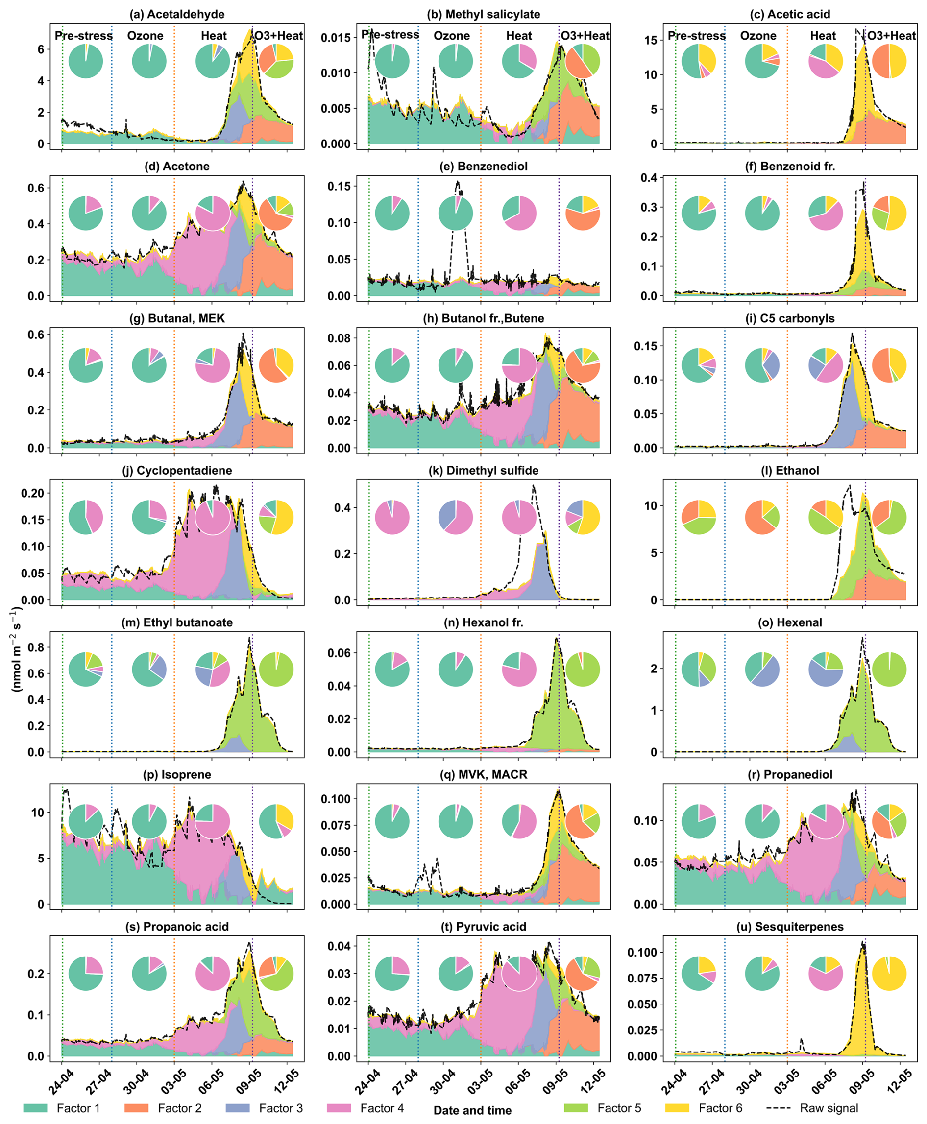
Figure B4 Stacked time series of PMF-resolved contributions for selected BVOC compounds during the Oak experiment. The black dashed lines indicate the original concentration of specific compounds, while stacked colored areas represent contributions from the six PMF-resolved factors. Each compound's emission is displayed across the four stress periods (Pre-stress, O₃ stress, O₃ + Heat stress, Heat stress), separated by vertical dashed lines. Inset pie charts show the relative contribution of each factor to compound emissions within each stress period, as a factor dominance.