Annual growth rates of column-averaged CO₂ inferred from Total Carbon Column Observing Network (TCCON)

Monitoring annual atmospheric CO₂ growth rates is a key constraint on assessing the long-term effectiveness of emission reduction strategies. We analyzed annual growth rates of column-averaged dry-air mole fractions of CO₂ (XCO₂) using long-term data from 12 sites within the Total Carbon Column Observing Network (TCCON), spanning four regions: the Arctic, two Northern Hemisphere midlatitude bands (40–50 and 30–40° N), and the Southern Hemisphere. While in situ ground-based measurements provide detailed records of near-surface CO₂ concentrations, XCO₂ reflects the column-averaged abundance across the entire atmosphere, offering a complementary perspective.

We compared TCCON-derived growth rates with ground-based in situ observations from the Mauna Loa Observatory (MLO). Three calculation methods – Monthly Mean (MM), Fourier Fit residuals (FF), and Dynamic Linear Model (DLM) – were evaluated, with particular attention to the Eureka site, where polar night introduces substantial data gaps. In addition, the Copernicus Atmosphere Monitoring Service (CAMS) reanalysis product was used to assess consistency with TCCON-based growth rates and to evaluate each method's robustness to missing data. Among the methods tested, the DLM approach proved most resilient to data gaps.

Regionally averaged CO₂ growth rates, calculated from 2010 or from the earliest available data through 2024, ranged from approximately 2.33 to 2.40 ppm yr⁻¹. The most prominent signal was associated with the 2015–2016 El Niño – Southern Oscillation (ENSO) event, during which growth rates increased by up to 1.7 ppm yr⁻¹. The impact of COVID-19-related emission reductions in 2020 was also examined: a decline of 0.4 ppm yr⁻¹ was observed in the 30–40° N region, whereas other regions showed no significant decline. Correlation analysis between growth rates and ENSO strength revealed significant relationships in the Southern Hemisphere and at Mauna Loa, but not in northern mid- or high-latitude regions.

1 Introduction

It is estimated that Earth's global surface temperature was more than 1 °C warmer in the decade 2011–2020 compared to pre-industrial levels (Lee et al., 2023). The rise in Earth's surface temperature has severe consequences, including sea level rise, extreme heat events, drastic shifts in precipitation patterns, and droughts, all of which pose significant risks to ecosystems and human societies (Lee et al., 2023). To mitigate these impacts and achieve the goals set by the Paris Agreement, limiting global temperature rise to 1.5 °C by 2050, there is an urgent need to drastically reduce anthropogenic greenhouse gas (GHG) emissions and reach net-zero CO₂ emissions (UNFCC, 2015; Lee et al., 2023).

Since the Industrial Revolution, anthropogenic CO₂ emissions have generally increased each year, but with occasional declines during major global events, such as the 2008 economic recession and the 2020 COVID-19 pandemic (Crippa et al., 2023). During these periods, economic slowdowns led to temporary reductions in CO₂ emissions. The COVID-19 pandemic, in particular, provides a unique opportunity to evaluate the atmospheric response to an abrupt and large-scale drop in emissions. In 2019, global CO₂ emissions were estimated at 37.8 Gt yr⁻¹ (Crippa et al., 2023). According to IPCC scenarios consistent with limiting warming to 1.5 °C, global GHG emissions must decline by approximately 84 % by 2050 relative to 2019 levels (Lee et al., 2023), implying steep reductions in gross emissions and/or increased CO₂ removal. This corresponds to an average annual reduction of approximately 1 Gt CO₂ yr⁻¹. Due to restrictions related to the COVID-19 pandemic, global fossil fuel CO₂ emissions in 2020 decreased by approximately 1.9 Gt compared to 2019 (Crippa et al., 2023), a drop nearly twice as large as this expected annual average. Understanding whether such reductions are detectable in atmospheric CO₂ concentrations is crucial for assessing the effectiveness of future emission reduction strategies.

Data from National Oceanic and Atmospheric Administration (NOAA) Global Monitoring Laboratory indicate that the annual CO₂ growth rate, as measured at the Mauna Loa Observatory, decreased by 8 % in 2020. However, this reduction is relatively small compared to the much larger increases observed during strong El Niño events, such as the 45 % increase in 2015–2016 (NOAA, 2024). This highlights the challenge of distinguishing between natural variability and anthropogenic emission changes. Moreover, monitoring atmospheric CO₂ concentrations across multiple regions is essential, as the detectability of emission-driven changes can vary due to differences in regional fossil fuel emissions, biospheric fluxes, and atmospheric transport patterns. For example, mid-latitude regions with high anthropogenic emissions may exhibit more immediate responses, while remote or high-latitude regions may show delayed or muted signals.

Several surface in-situ observation sites around the world monitor CO₂ concentrations in the atmosphere, however, surface measurements are more sensitive to local emissions, especially when observation sites are located near high-emission regions, and they are greatly affected by boundary layer dynamics. Total column observations, on the other hand, are less sensitive to local emissions and more representative of regional emissions (Keppel-Aleks et al., 2011). Given their larger spatial footprints, total column measurements provide more information for inverse modeling of regional emissions and trends. Moreover, with advancements in remote sensing techniques from space, column-averaged dry–air mole fraction of CO₂ can now be measured in remote regions, enabling broader spatial coverage.

The Total Carbon Column Observing Network (TCCON) with 28 stations across four continents, provides long-term ground-based remote sensing observations of CO₂ that are also widely used for validating satellite measurements (Wunch et al., 2010). Satellite missions, such as GOSAT and OCO-2, have been measuring total column CO₂ from space since 2009 and 2014, respectively (Yokota et al., 2009; Crisp, 2015), significantly enhancing global monitoring of CO₂ levels in the atmosphere. These satellite datasets have also been incorporated into the Copernicus Atmosphere Monitoring Service (CAMS), which assimilates measurement data to produce CO₂ flux estimates and gapless total column mole fractions all over the world (Agustí-Panareda et al., 2023).

In-situ networks, TCCON, satellite observations, and CAMS reanalysis all offer valuable datasets for investigating CO₂ growth rates across different regions of the world. Several studies have employed ground-based and space-based total column data to examine CO₂ trends and their driving factors. For instance, Lindqvist et al. (2015) compared CO₂ column mole fractions from the GOSAT satellite with measurements from various TCCON stations, providing insights into the seasonal and interannual variability of atmospheric CO₂. Sussmann and Rettinger (2020) developed a framework for deriving annual growth rates from TCCON column-averaged dry-air mole fractions of carbon dioxide (XCO₂) and estimating uncertainties. They applied this method to assess the detectability of COVID-19-related CO₂ emission reductions, highlighting the challenge of distinguishing small anthropogenic signals from natural variability. Buchwitz et al. (2018) used an ensemble-based satellite product to calculate annual CO₂ growth rates both globally and by latitude bands, later refined with updated measurements and an improved ensemble version (Reuter et al., 2020). Extending this work, Labzovskii et al. (2021) analyzed CO₂ growth rates derived from 24 TCCON stations and compared them to results from CarbonTracker, CAMS reanalysis, and satellite-based estimates by Reuter et al. (2020). Collectively, these studies demonstrate how integrating TCCON and satellite data products enhances our understanding of interannual variability in CO₂ growth rates across different regions.

In this study, we aim to quantify and interpret regional differences in atmospheric CO₂ growth rates using long-term TCCON total column measurements, in-situ observations, and CAMS reanalysis data. Specifically, our objectives are to:

• 1.

  evaluate and compare three established methods for estimating annual CO₂ growth rates, identifying the most robust approach for datasets with irregular sampling;

• 2.

  investigate how interannual variability – particularly associated with Southern Oscillation (ENSO) events – and anthropogenic emission changes, such as the 2020 COVID-19-related reduction, influence observed CO₂ growth rates across regions. Building on Sussmann and Rettinger (2020), this work extends the temporal coverage to include the year 2020, expands the analysis to additional TCCON stations across four latitude bands (30–50° N, Arctic, and Southern Hemisphere), and integrates reanalysis data to evaluate methodological and regional differences in CO₂ growth-rate behavior.

Section 2 offers an overview of the measurement sites and modeled products utilized in this study. In Sect. 3, we provide a brief introduction to three methods for calculating annual growth rates and describe their application to our datasets. Section 4 presents the results of the growth rate calculation method analysis, along with the calculated growth rates for each study region based on the most effective method. Finally, Sect. 5 discusses the implications of our findings and explores potential future applications of this analysis.

2 Data

In this analysis, we use XCO₂ measurements from 12 TCCON sites and surface CO₂ in-situ observations from Mauna Loa Observatory (MLO) to compare CO₂ growth rate trends. Although the focus of this study is on total column measurements, MLO is included due to its long-term record, its central role in global CO₂ growth rate assessments (e.g., NOAA's Global Monitoring Laboratory (NOAA GML), UK Met Office analyses (Betts et al., 2024)). In addition its high-altitude location, makes it more representative of the free troposphere and therefore more comparable to total column observations.

In addition, we include a gridded modeled total column CO₂ product from the CAMS Reanalysis (Agustí-Panareda et al., 2023; Chevallier, 2024), which assimilates satellite retrievals from OCO-2 together with surface and aircraft observations to provide spatially and temporally continuous estimates of atmospheric CO₂. The CAMS dataset has a spatial resolution of 1.4°×0.7° and a 3 h temporal resolution, spanning from 2014 to 2023. This product is used for comparison with the observational data and offers the advantage of continuous global coverage that complements the sparser ground-based network. However, because it is produced through data assimilation, it may smooth fine-scale variability and reflect assumptions inherent in the underlying transport model and flux priors. Nevertheless, its continuous and gap-free nature makes it particularly valuable for testing the sensitivity of growth-rate estimation methods and for quantifying the impact of data gaps on trend calculations.

2.1 In-Situ Measurement Site

The Mauna Loa Observatory provides the longest continuous atmospheric CO₂ record, initiated by the Scripps Institution of Oceanography in 1958 and complemented by NOAA's GML, which has conducted continuous in-situ measurements since 1974 (Lan et al., 2025; Thoning et al., 2024). For this study, we use the continuous in-situ dataset from NOAA/GML at MLO, which is widely employed for calculating annual growth rates. For example, the UK Met Office uses Mauna Loa data to forecast annual CO₂ growth rates within their seasonal-to-decadal climate models (Betts et al., 2024).

2.2 TCCON Sites

We utilize the XCO₂ data from 12 TCCON sites, the column-averaged dry-air mole fraction of CO₂ retrieved using the GGG software by profile scaling (TCCON Team, 2020; Laughner et al., 2024). The a priori profiles are constructed using meteorological data from the Goddard Earth Observing System Forward Processing for Instrument Teams (GEOS-FP-IT) atmospheric data assimilation system (Lucchesi, 2013). TCCON column retrievals are scaled to the World Meteorological Organization (WMO) trace gas scale using aircraft- or balloon-based measurements (Laughner et al., 2024).

To investigate the atmospheric response to changes in anthropogenic CO₂ emissions, we choose a subset of TCCON stations in various regions. Recognizing that the majority of fossil fuel emissions occur in the mid-latitudes of the Northern Hemisphere (30–50° N) and considering the latitudinal gradient in CO₂ we choose three stations in each of the two different latitude bands 40–50 and 30–40° N. We also choose three stations in the high Northern latitudes to investigate the growth rate in the Arctic region. In addition, we consider three stations in the Southern Hemisphere where CO₂ growth is largely influenced by transport from the Northern Hemisphere (Dargaville et al., 2003). From each region, we select sites that are not located in highly urbanized areas, have at least five years of observations, and include data extending to 2020, ensuring a sufficient number of data points for robust growth rate trend analysis.

Strong et al. (2022)Buschmann et al. (2022)Kivi et al. (2022)Sussmann et al. (2025)Wennberg et al. (2022a)Morino et al. (2022)Wennberg et al. (2022b)Iraci et al. (2022)Shiomi et al. (2022)Deutscher et al. (2023b)Deutscher et al. (2023a)Pollard et al. (2022)Thoning et al. (2024)Chevallier et al. (2023)

Table 1 TCCON, in-situ, and CAMS data used for CO₂ growth rate calculation: site locations, measurement periods and average number of measurements per year.

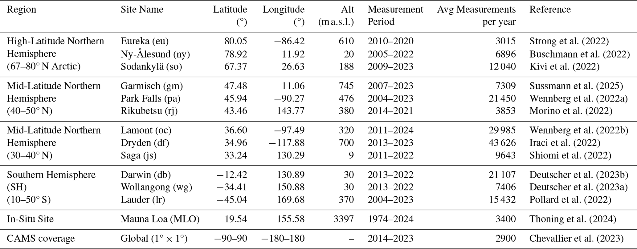
We choose three sites from higher latitudes in the Northern Hemisphere (67–80° N): 1. Sodankylä, a rural area located in Northern Finland (Kivi et al., 2022; Kivi and Heikkinen, 2016); 2. Ny-Ålesund, which hosts AWIPEV Arctic Research Base (Alfred Wegener Institute for Polar and Marine Research and the French Polar Institute Paul-Émile Victor) on the Svalbard Norwegian island in northern Europe (Buschmann et al., 2022); and 3. Eureka located in Nunavut, which hosts the Polar Environment Atmospheric Research Laboratory (PEARL) (Strong et al., 2022).

For the Northern latitude bands 40–50° North, we choose 1. Park Falls located in Wisconsin USA, within the boreal forest (Wennberg et al., 2022a), 2. Garmisch, located in a small town in Southern Germany in the foothills of the Alps (Sussmann et al., 2025); and 3. Rikubetsu in the island of Hokkaido, Northern Japan, positioned in a rural, mountainous region (Morino et al., 2022).

For the Northern latitude bands 30–40° N, we choose 1. Dryden, California, USA, at the NASA Armstrong Flight Research Center (AFRC) on Edwards Air Force Base (Iraci et al., 2022), desert area, located 150 km northeast of Los Angeles. 2. Lamont, a rural area located in Southern Great Plains in Oklahama, USA (Wennberg et al., 2022b). 3. Saga, a small town located in the island of Kyushu in Southern Japan (Shiomi et al., 2022).

The three Southern Hemisphere stations that meet our time series criteria are: 1. Darwin, Australia, located in Northern Australia (Deutscher et al., 2023b); 2. Wollongong, located in Southeast Australia (Deutscher et al., 2023a); and 3. Lauder, located on New Zealand's South Island (Pollard et al., 2022). Although these stations fall within different latitude bands, the relatively subdued variability in CO₂ levels across the Southern Hemisphere enables meaningful comparisons of CO₂ growth trends by combining data from these locations (Stephens et al., 2013). Data from Darwin and Wollongong are available starting in 2013, while Lauder provides an earlier record beginning in 2010. The 2010–2012 Lauder record used here was provided privately and is not included in the publicly available TCCON files. Accordingly, Lauder is used exclusively to estimate growth rates for 2011–2013, and from 2014 onward, all three sites are included in the Southern Hemisphere average.

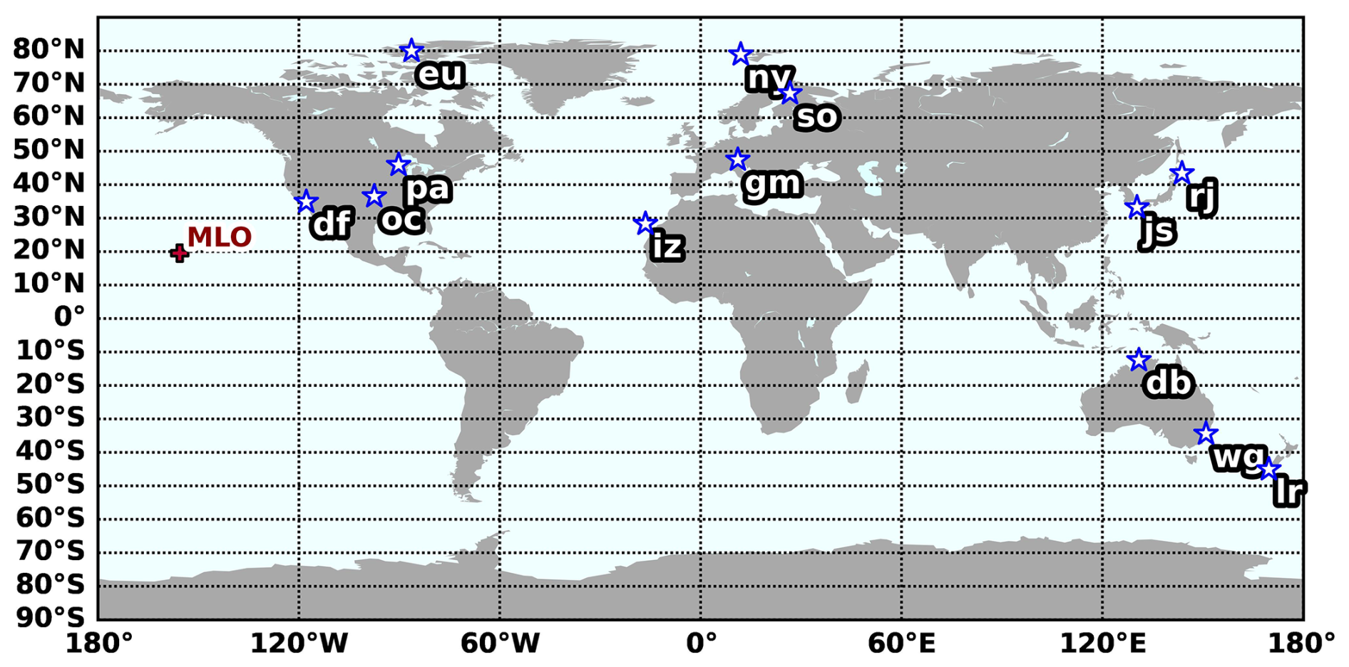
Figure 1 Selected TCCON stations used in this study (marked by white stars). High–latitude NH sites: eu (Eureka), ny (Ny-Ålesund), so (Sodankylä). 40–50° N latitude band: gm (Garmisch), pa (Park Falls), rj (Rikubetsu), 30–40° N Latitude band: oc (Lamont), df (Dryden) , js (Saga). Southern Hemisphere sites db (Darwin), wg (Wolangong), lr (Lauder) are marked by white stars. The in situ measurement site, Mauna Loa Observatory (MLO), is indicated by a red cross. Global map based on Natural Earth public domain data and plotted using the Cartopy Python library (Met Office, 2024; Natural Earth, 2025).

Table 1 summarizes the measurement sites used in this study, including their geographic locations, measurement periods, and the average number of individual measurements per year as an indicator of data availability. TCCON measurements are based on roughly 2 min acquisition intervals and are only taken when sunlight is available, whereas Mauna Loa data consist of hourly averages collected continuously, independent of weather or time of day. Consequently, the number of data points from Mauna Loa is substantially lower. The geographic distribution of the selected sites is shown in Fig. 1.

2.3 Modelled Reanalysis Product

CO₂ growth rates derived from TCCON measurements may be affected by biases when significant temporal gaps occur, as TCCON retrievals require direct sunlight and cannot be performed under cloudy conditions or at night. In high-latitude regions, extended periods of low solar elevation or polar night can result in full seasonal gaps, further increasing the risk of biases in annual growth rate estimates.

To evaluate the potential impact of these data gaps, we use the CAMS reanalysis product as a complementary dataset (Agustí-Panareda et al., 2023; Chevallier, 2024). Its spatiotemporal continuity enables us to simulate the effect of TCCON sampling patterns on annual growth rate estimates and to assess the sensitivity of different growth-rate calculation methods to irregular data availability.

3 Methods

Accurately calculating annual CO₂ growth rates is critical for understanding atmospheric trends and identifying regional differences. In this study, we evaluate three commonly used methods to assess their robustness and sensitivity to data gaps, particularly at sites with limited observational coverage. A sensitivity analysis is performed to examine how data availability affects growth rate estimates by applying these methods to both TCCON measurements and CAMS satellite reanalysis data at sites with the most pronounced data gaps. Finally, we apply the most reliable method, based on this evaluation, to the regionally averaged time series for each study region.

3.1 Data Preparation

For TCCON, we use the publicly available dataset processed with GGG2020 (TCCON Team, 2020; Laughner et al., 2024), excluding CO₂ measurements with errors exceeding 3 ppm to ensure high data quality. The only exception is the 2010–2012 Lauder record, which was provided privately by the site principal investigator. For MLO in-situ measurements, only observations classified as valid according to the NOAA three-character quality control flag were included in the analysis. These datasets differ in temporal resolution: TCCON provides measurements every 2 min whenever sufficient solar radiation is available, MLO data are reported hourly, and CAMS reanalysis offers continuous, gap-free data at 3 h intervals.

To mitigate random noise and represent atmospheric variability on synoptic scales, we aggregate the data into weekly averages following the approach of Sussmann and Rettinger (2020). To ensure consistency, we analyze TCCON and MLO data starting from 2010 and align comparisons with CAMS reanalysis data from 2014 onward. For spatial consistency, we use the CAMS grid point nearest to each TCCON site.

The resulting weekly time series for each TCCON site dataset, as well as the regional averages, are shown in Fig. A1, illustrating the differences in sampling frequency and data coverage across sites. Regional growth rates are calculated by averaging the weekly time series from stations within each region, which reduces the influence of outliers, increases sampling density, and thereby decreases statistical uncertainty in the regional growth rate estimates. This results in narrower confidence intervals and a more representative, stable regional trend. Although data availability varies across sites – sometimes causing unequal contributions – combining multiple stations overall improves estimate robustness.

3.2 Growth Rate Calculation Methods

We examine three previously established methods to estimate annual CO₂ growth rates: the Monthly Mean (MM), Fourier Fit residuals (FF), and Dynamic Linear Model (DLM). The growth rate here refers to the increase in atmospheric CO₂ concentration, expressed in parts per million per year (ppm yr⁻¹), calculated over a one-year period. Each method is applied to weekly averaged data to minimize short-term variability and to maintain consistency across datasets with differing temporal resolutions. These three methods were selected based on their prior use in similar studies (Buchwitz et al., 2018; Sussmann and Rettinger, 2020; Hachmeister et al., 2024) and their suitability for datasets with varying temporal coverage and data density.

3.2.1 Monthly Mean (MM)

The Monthly Mean (MM) method, originally introduced by Buchwitz et al. (2018) for satellite observations and later applied to TCCON ground-based measurements by Labzovskii et al. (2021), estimates annual growth rates by first computing the average CO₂ value for each calendar month m (e.g., January, February, etc.) in each year y, denoted as C_y,m. This yields up to 12 monthly averages per year. Monthly growth rates are then calculated by differencing the same months from consecutive years, i.e., $\mathrm{\Delta }{C}_{y,m}=C_{y,m}-C_{y-\mathrm{1},m}$. The annual growth rate for year y is then obtained by averaging the available monthly growth rates as

$$\begin{array}{}\text{(1)}& {\text{gr}}_y={\displaystyle \frac{\mathrm{1}}{N_y}}\sum _{m=\mathrm{1}}^{N_y}\mathrm{\Delta }{C}_{y,m}\end{array}$$

where N_y is the number of months with valid data in both year y and year y−1. The associated uncertainty is estimated by calculating the standard deviation σ_y of the ΔC_y,m values and scaling it to account for incomplete month coverage, i.e., $\mathit{\delta }{\text{gr}}_y={\mathit{\sigma }}_y\cdot \sqrt{\mathrm{12}/N_y}$. This method is valued for its simplicity and ease of implementation; however, it is sensitive to data gaps, as missing months may reduce N_y and potentially introduce biases in the estimated annual growth rates.

3.2.2 Fourier Fit (FF)

The Fourier Fit (FF) method combines linear regression with a Fourier series to model the long-term trend and seasonal cycle in CO₂ time series, as described by Sussmann and Rettinger (2020). The fit is expressed as $F(t,a_{\mathrm{0}},a_{\mathrm{1}},b_{\mathrm{1}},\mathrm{\dots },b_{\mathrm{8}})$, where a₀ is the intercept, a₁ is the slope of the linear trend, and b₁ to b₈ are the Fourier coefficients for four annual harmonics. The residuals are calculated as the difference between the measured CO₂ values M and the model fit: M−F(t). These residuals represent deviations from the overall trend at each time step and are used to quantify annual offsets.

For each year, a constant offset a_0,yr is fitted to the residuals, representing how that year's median deviates from the overall fit. The annual growth rate is then calculated as the difference in these offsets between consecutive years, added to the linear trend term a₁, as follows:

$$\begin{array}{}\text{(2)}& {\text{gr}}_{\text{yr}}=a_{\mathrm{0},\text{yr}}-a_{\mathrm{0},\text{yr}-\mathrm{1}}+a_{\mathrm{1}}\end{array}$$

This formulation captures both the long-term linear increase in CO₂ and interannual deviations from the trend. Confidence intervals are estimated using bootstrap resampling with 5000 iterations, following Sussmann and Rettinger (2020), with the 2.5th and 97.5th percentiles defining the 95 % confidence interval.

3.2.3 Dynamic Linear Model (DLM)

The Dynamic Linear Model (DLM) is a statistical framework well suited for analyzing time series with irregular sampling and data gaps. For example, Laine (2020) applied it to analyze ozone trends in the atmosphere, and later adapted for satellite-based methane retrievals by Hachmeister et al. (2024). For this analysis, we use the “dlmhelper” package developed by Hachmeister (2025), which streamlines the application of Dynamic Linear Model (DLM) in atmospheric datasets.

We determine the best-fit model from an ensemble of DLMs with different numbers of harmonic components (1, 2, 3, or 4), selecting the configuration that yields the lowest total covariance level. In most regions, the best performance is obtained using four harmonics, while in the Arctic region, only one harmonic is selected, as the extended winter data gaps limit the stability of higher-order harmonics and may lead to overfitting.

We apply the DLM to fit weekly time series of XCO₂, providing estimates of the underlying CO₂ levels at that temporal resolution. The DLM method provides a fit on the same temporal resolution as the input data, so using weekly input results in a weekly-resolved growth rate time series. From this, we calculate annual growth rates as the difference between deseasonalized annual means of the DLM fit in consecutive years:

$$\begin{array}{}\text{(3)}& {\text{gr}}_{\text{yr}}^{\text{DLM}}={\mathit{\mu }}_{\text{yr}}-{\mathit{\mu }}_{\text{yr}-\mathrm{1}}\end{array}$$

where μ_yr is the mean of the deseasonalized, detrended DLM fit for year yr. The associated uncertainty in each annual growth rate is estimated as the square root of the sum of the annual level covariances from adjacent years, i.e., ${\mathit{\sigma }}_{\text{gr},\text{yr}}^{\text{DLM}}=\sqrt{{\mathit{\sigma }}_{\mathit{\mu },\text{yr}}^{\mathrm{2}}+{\mathit{\sigma }}_{\mathit{\mu },\text{yr}-\mathrm{1}}^{\mathrm{2}}}$. Uncertainties tend to be larger at the beginning and end of the time series due to edge effects, as the DLM has fewer observations to constrain the model at the boundaries.

A visual comparison of the three methods and their respective definitions of growth rate is shown in Fig. A2.

3.2.4 Method Evaluation and Selection

To assess the robustness of the three methods, we evaluate them at three sites with varying data coverage. Mauna Loa (MLO) offers high-quality, near-continuous hourly in-situ measurements, including nighttime observations. Lamont, a TCCON site located in a region with frequent sunlight, provides a dense and consistent dataset. In contrast, Eureka, a high-latitude TCCON site, experiences sparse measurements a pronounced data gap during the polar night in winter due to the absence of sunlight.

To evaluate the impact of such data gaps in a high-latitude context, we conduct a sensitivity analysis at Eureka using the gap-free CAMS reanalysis dataset. Growth rates are first calculated using the complete CAMS time series, then recalculated after downsampling the dataset to match the temporal coverage of the TCCON measurements. This comparison reveals the method most resilient to missing data, which is subsequently applied to the regionally averaged TCCON time series across the four study regions.

4 Results

4.1 Growth rate calculation method comparison

To evaluate the performance of different growth rate calculation methods, we applied three approaches to the three representative sites selected in Sect. 2.2. We used all available data from 2009 onward, allowing annual growth rates to be derived starting in 2010. Figure A3 displays the time series of measurements from the three stations. The MLO in-situ measurements cover the entire period, except for a gap from December 2022 to 4 July 2023, caused by the Mauna Loa Volcano eruption (Thoning et al., 2024). Lamont TCCON measurements began in April 2011, allowing for annual growth rate calculations from 2012 onward. Eureka has data available from 2010, but there are no measurements for 2012 and 2013. Furthermore, measurements were interrupted in July 2020 because of instrument issues that could not be addressed due to COVID-19 travel restrictions, limiting growth rate calculations to data available through 2020.

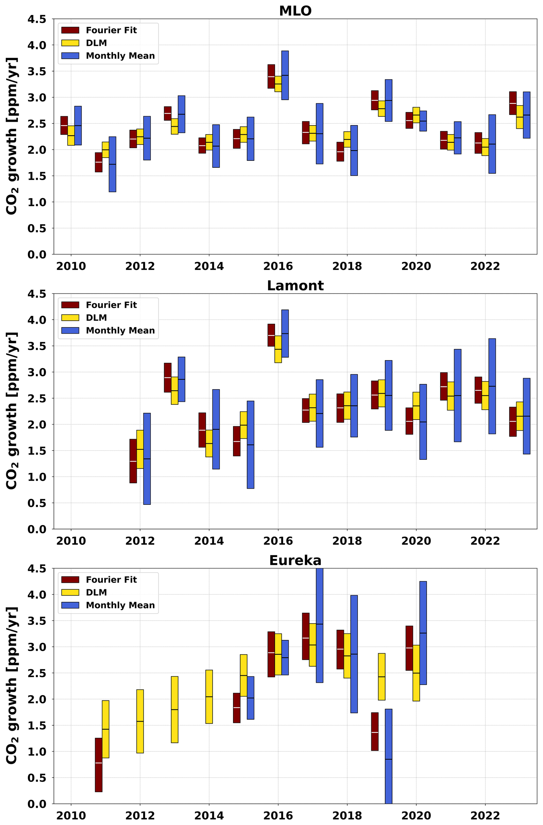
Figure 2 Annual CO₂ growth rates are plotted by year for each of the three sample sites using three different methods. The central line within each bar indicates the median growth rate, and the bar length reflects the associated uncertainty, which is defined separately for each method.

Figure 2 presents annual growth rate estimates and the associated uncertainty ranges at each station using the three different methods. While each method uses its own approach to estimate uncertainties, a qualitative comparison shows that the Monthly Mean method tends to produce broader uncertainty ranges, making it more difficult to resolve year-to-year changes. By contrast, the Fourier Fit and DLM methods yield comparatively smaller uncertainty ranges, as evaluated within each method's framework. The uncertainty in the annual growth-rate estimates also depends on the number of available observations, with larger confidence intervals occurring in years or sites with fewer measurements.

At Eureka, the DLM interpolates growth rates during the 2012–2014 gap. However, these estimates must be interpreted with caution, as they rely on the assumption of smooth variation, and cannot capture potential short-term fluctuations similar to those seen at Lamont and MLO during that period.

At MLO and Lamont, the growth rates from all three methods show close agreement. At Eureka, a notable discrepancy appears in 2019 between the DLM estimate and the other two methods, possibly due to data sparsity at this station. The following section explores the sensitivity of each method to data gaps in more detail.

4.1.1 Gap sensitivity analysis

Figure A4 presents the CAMS reanalysis XCO₂ time series overlaid with TCCON measurements at Eureka. This overlay demonstrates the practical advantage of using CAMS in Arctic regions, where TCCON observations are frequently unavailable due to polar night or instrument downtime. To assess whether the observed differences in growth rate estimates between TCCON and CAMS stem from actual variability or are primarily driven by data availability, the CAMS dataset was downsampled to match the temporal coverage of the TCCON measurements.

To perform the downsampling, the high-frequency TCCON data were first averaged into 3 h means to match the native temporal resolution of the CAMS reanalysis. Next, both time series were merged by timestamp, and only 3 h intervals where both TCCON and CAMS had valid data were retained. This allowed the CAMS dataset to be filtered such that its temporal coverage mirrored that of TCCON. The resulting downsampled CAMS data were then averaged into weekly means – consistent with the treatment of other datasets – prior to applying the growth rate calculation methods. The downsampled CAMS time series is also included in Fig. A4 for reference. The analysis period was restricted to 2014 onward to match the start date of the CAMS reanalysis product.

For both the TCCON and downsampled CAMS datasets, the DLM ensemble member with the lowest level covariance corresponded to a configuration with only one seasonal parameter, which we selected for our analysis. Similarly, for the FF method, we initially applied four harmonics as used for other stations, but significant data gaps in the Eureka record led to overfitting. To improve the stability of the fit and align with the DLM configuration, we reduced the model to a single seasonal parameter. The MM method does not involve curve fitting and instead relies on the available monthly data. Due to the relatively sparse measurements at Eureka, the MM approach resulted in broader uncertainty ranges reflecting the smaller sample size.

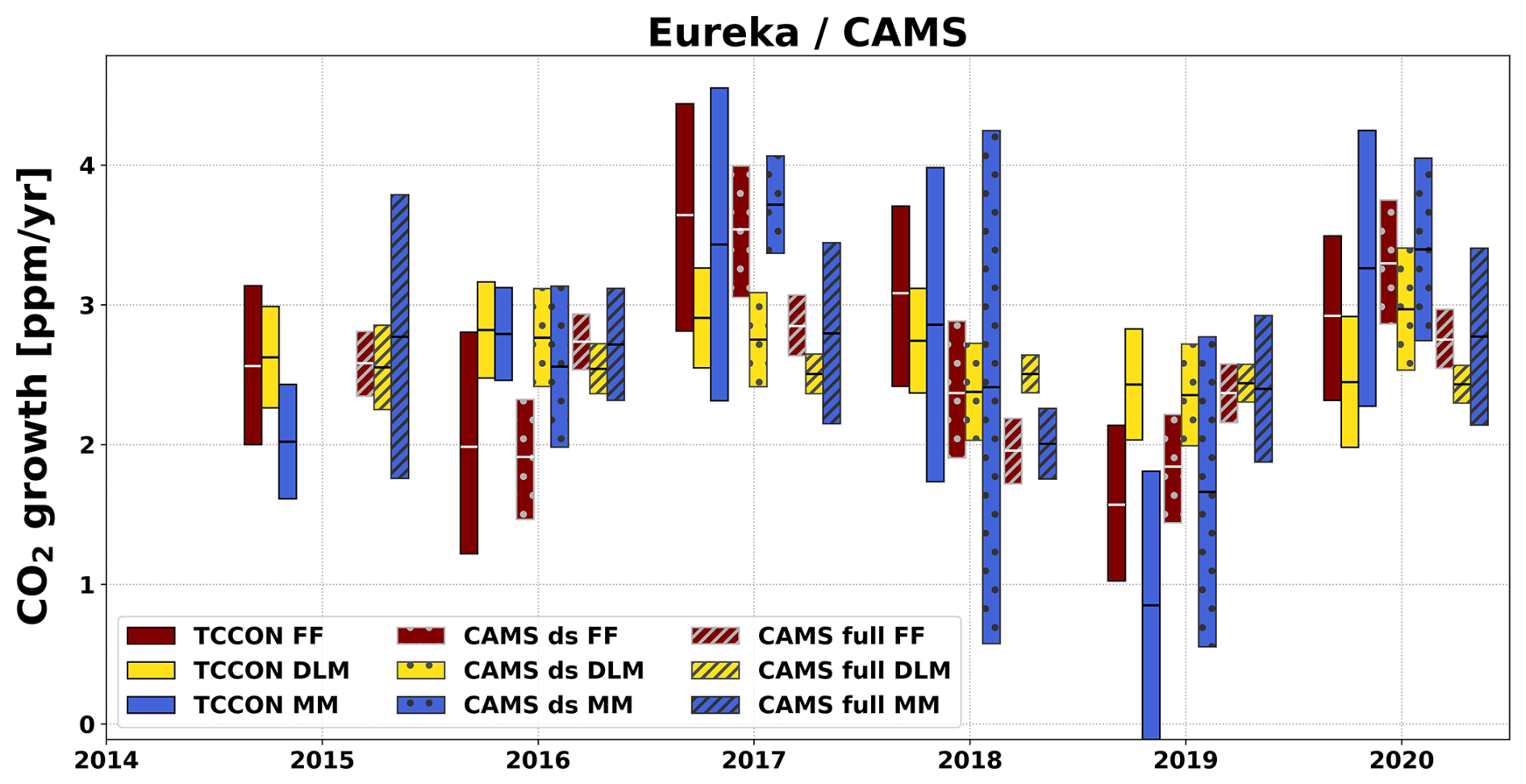
Figure 3 Annual CO₂ growth rates plotted for Eureka and the closest CAMS grid point original and downsampled (ds) to match the TCCON measurements, using the three approaches for calculating growth rate. The x-axis represents calendar years. The central line within each bar indicates the median growth rate, and the bar length reflects the associated uncertainty, which is defined separately for each method.

Figure 3 illustrates the annual CO₂ growth rates at Eureka, derived from both TCCON measurements and CAMS reanalysis data. For the TCCON dataset (solid bars), all three methods produce broadly consistent growth rates, except for 2019, as noted earlier. The MM method (blue) shows larger uncertainties, in line with its statistical formulation, making it less sensitive to interannual variability. In contrast, the DLM (yellow) and FF (maroon) methods exhibit sharper year-to-year changes.

When applied to full-resolution CAMS data, all three methods agree well within uncertainty across all years (hatched bars). For the downsampled CAMS dataset (dotted bars), which mimics TCCON's temporal availability, the absence of data in 2014 prevents growth rate calculation for 2015. In subsequent years, the FF and MM methods exhibit noticeable shifts in mean growth rates compared to full-resolution CAMS, particularly in 2016–2017 – suggesting these methods are more sensitive to sampling density. The DLM method appears least affected by downsampling, with results (dotted yellow) staying within the envelope of both the full CAMS and TCCON estimates, including in 2019.

In 2019, which was previously identified as a year with atypical behavior in the TCCON dataset, the DLM method remained notably stable across all datasets, indicating greater robustness to data irregularities and gaps. In contrast, the FF and MM methods exhibited shifts more strongly influenced by irregular sampling. The MM method has the advantage of being computationally simple and performs reasonably well in the presence of moderate data gaps, but it lacks the resolution needed to capture interannual variability. The FF method generally produces uncertainty ranges comparable to those of the DLM but is computationally intensive due to the bootstrap resampling procedure. The DLM method, while also computationally demanding because of ensemble fitting and model selection, offers the greatest stability and reliability, particularly for remote-sensing datasets with discontinuous temporal coverage. For this reason, we adopt the DLM method for investigating CO₂ growth rates across different regions.

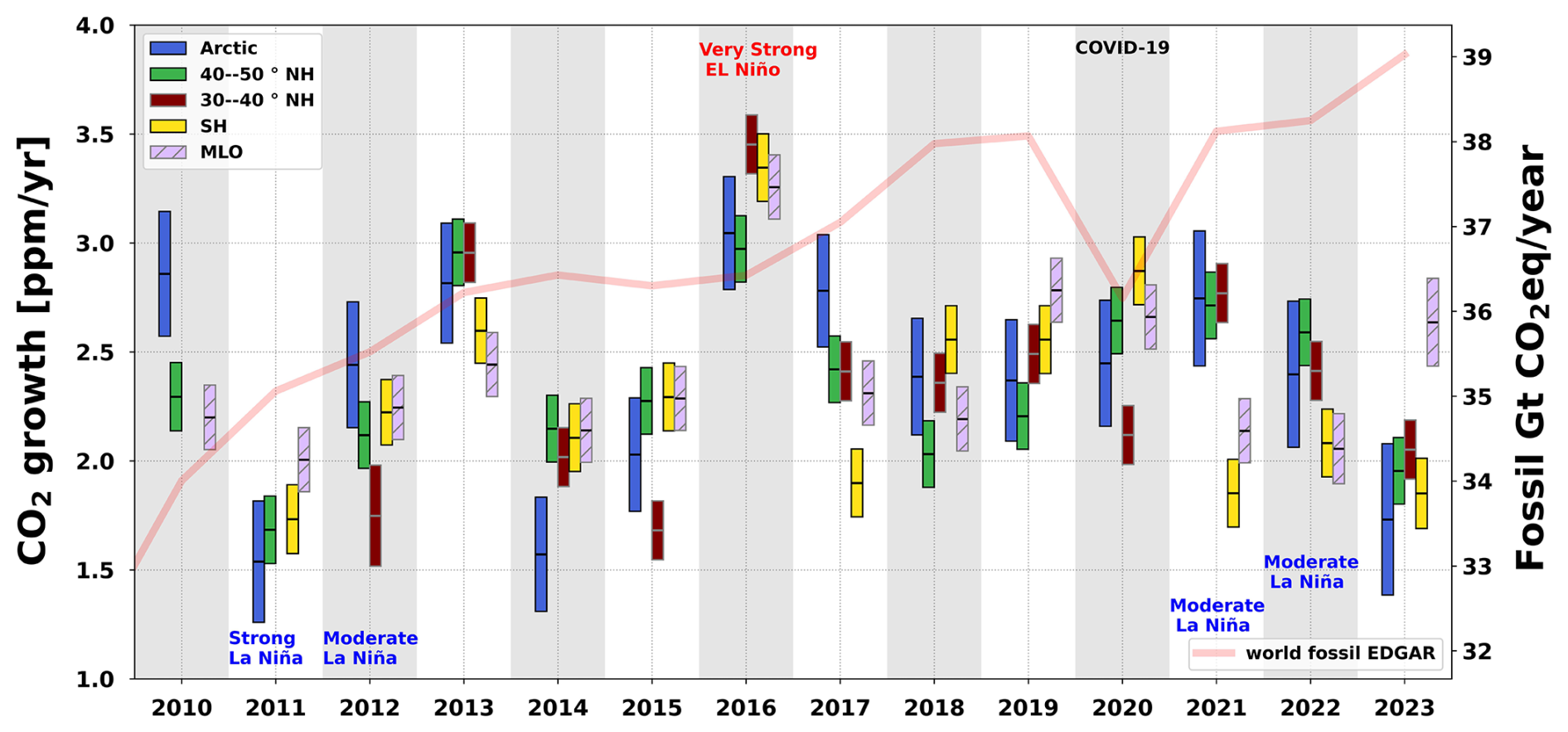
Figure 4 Annual growth rates and their uncertainty ranges for the four TCCON regions and MLO, calculated using the DLM method shown by year. The central line within each bar indicates the median growth rate, and the bar length reflects the associated uncertainty. The red line represents global fossil fuel CO₂ emission trends from EDGAR.

4.2 Interannual variations in CO₂ growth rates

Figure 4 illustrates the interannual variations in CO₂ growth rates across the four TCCON study regions and the MLO in situ site, overlaid with fossil fuel emissions from the Emissions Database for Global Atmospheric Research (EDGAR) database (Crippa et al., 2023). Detailed annual growth rates for individual sites within each region are provided in Fig. A5.

Overall, CO₂ growth rate trends show broad agreement across regions, despite year-to-year variability. Long-term average growth rates are remarkably similar – around 2.4 ppm yr⁻¹ – for the Arctic, 30–40° N, 40–50° N, and MLO in situ, with uncertainties ranging from ± 0.3 to ± 0.5 ppm yr⁻¹. The Southern Hemisphere shows a growth rate of 2.3 ± 0.6 ppm yr⁻¹. The reported uncertainties represent the standard deviation of annual growth rates, reflecting interannual variability. The overlapping uncertainty ranges indicate consistent long-term CO₂ growth trends across these spatial domains.

Table 2 Annual CO₂ growth rate anomalies (ppm yr⁻¹, with percentage change relative to the previous year in parentheses) for various regions and the Mauna Loa Observatory (MLO), shown alongside fossil fuel emission changes (from EDGAR) and ENSO classifications. Statistical significance is based on non-overlapping uncertainty ranges; strongly significant anomalies are highlighted in bold.

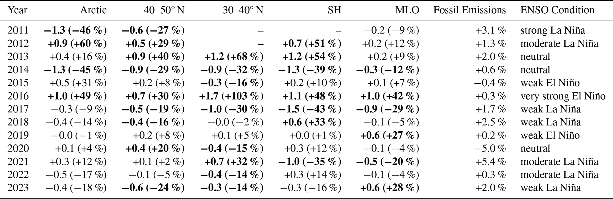
To better illustrate the interannual variability, Table 2 presents the CO₂ growth rate anomalies alongside ENSO conditions and fossil fuel emission changes. In 2016, a year marked by a strong El Niño event, all regions exhibited statistically significant increases in CO₂ growth rates compared to 2015, with most sites showing large absolute increases exceeding 1 ppm yr⁻¹. An exception is the 40–50° N region, which showed a smaller but still statistically significant increase of +0.7 ppm yr⁻¹. The strong El Niño event in 2016 led to enhanced CO₂ growth rates globally due to widespread drought and fire activity that reduced biospheric uptake. The weaker response observed at 40–50° N likely reflects the reduced sensitivity of mid-latitude ecosystems to ENSO-driven climate anomalies, consistent with findings by Zhang et al. (2019), who reported that ENSO and gross primary production (GPP) coupling is strongest in tropical and arid regions and weaker or lagged in temperate and boreal zones.

In 2020, following a notable 5 % reduction in fossil fuel CO₂ emissions, a distinct divergence in growth rates is observed across regions. While the MLO site shows only a slight decline compared to 2019, the Arctic and Southern Hemisphere exhibit modest increases that fall within the range of interannual variability and are not statistically significant. In contrast, the 40–50° N region shows a statistically significant increase in growth rate, whereas the 30–40° N region experiences a significant but modest decrease of −0.4 ppm yr⁻¹ relative to 2019. Given the substantial drop in anthropogenic emissions, the decrease in the 30–40° N latitude band likely reflects its regional sensitivity to reduced fossil fuel activity – an effect not clearly observed elsewhere. This interpretation is supported by fossil fuel emission maps from EDGAR (Fig. A6), which show that the majority of anthropogenic CO₂ emissions occur within the 30–40° N latitude band that encompasses large urban and industrial areas. In contrast, the 40–50° N band includes more biosphere-dominated regions, where CO₂ variability is influenced primarily by temperature-driven changes in uptake. Consequently, the contrasting behavior between these two bands likely reflects differences in the dominant drivers of CO₂ variability, with additional contributions from region specific differences.

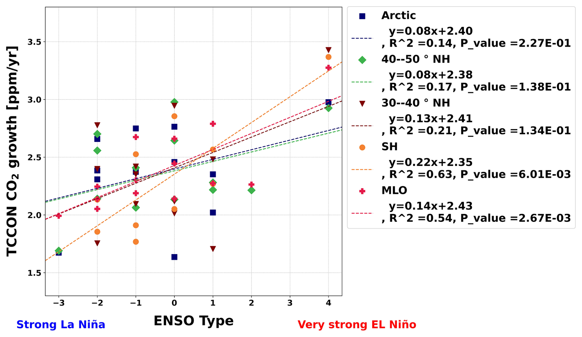
Figure 5 Correlation between TCCON calculated growth rates in four regions and MLO growth rates vs the ENSO strength each year as defined by NOAA.

The plot also highlights the influence of strong and moderate La Niña events on regional CO₂ growth rate patterns. In 2011, during a strong La Niña, a statistically significant decline in growth rates is observed in the 40–50° N region and the Arctic. This was followed by a moderate La Niña in 2012, after which all regions experienced increases in growth rates, likely reflecting a rebound from the preceding strong La Niña. In 2013, northern mid-latitudes saw growth rates rise by an additional 0.8–1.2 ppm yr⁻¹ relative to 2012. These increases are possibly the result of the combined effects of the transition out of the two-year La Niña phase and a concurrent rise in anthropogenic CO₂ emissions, which followed a steady upward trajectory between 2010 and 2013.

A similar pattern is observed during the 2021–2022 La Niña period: CO₂ growth rates declined at MLO and in the Southern Hemisphere, while the Arctic and northern high latitudes showed little change in 2021. Notably, the 30–40° N region exhibited a statistically significant increase that year, likely reflecting a rebound in fossil fuel emissions after the COVID-19 reductions. However, by 2022, the continued La Niña conditions appear to have exerted a broader suppressive effect on CO₂ growth rates across multiple regions. This declining trend persisted into 2023 for all TCCON regions, with particularly significant decreases in the 30–40 and 40–50° N latitude bands, while MLO showed a rebound. These results highlight the spatial heterogeneity of biospheric and atmospheric responses to ENSO variability and suggest the need for further analysis to better understand the underlying mechanisms.

Figure 5 further explores the relationship between ENSO strength and the calculated CO₂ growth rates in each region. Positive ENSO values correspond to El Niño events, while negative values indicate La Niña conditions. We adopt the ENSO strength classification used by Labzovskii et al. (2021), which ranges from −3 for strong La Niña to +4 for very strong El Niño, consistent with the Oceanic Niño Index (ONI) classifications provided by NOAA (https://ggweather.com/enso/oni.htm, last access: 21 July 2025). To account for the lag between oceanic temperature anomalies and their influence on the carbon cycle, we associate the second year of each two-year ENSO phase with the atmospheric response. This lag reflects the time needed for sea surface temperature changes to affect biospheric activity and CO₂ fluxes.

The correlation analysis reveals no statistically significant relationship between ENSO strength and CO₂ growth rates in the Arctic, 40–50° N, or 30–40° N regions (P-values > 0.05). In contrast, significant correlations with low P-values and high R² values are found for the Southern Hemisphere and MLO, suggesting a stronger sensitivity to ENSO-driven variability in these regions.

5 Conclusions

TCCON provides a valuable dataset for investigating regional CO₂ growth rates globally. While TCCON measurements offer precise and consistent data, regional variations in station coverage introduce uncertainties, particularly in areas with sparse or intermittent observations. Using multiple stations within a region increases data density, helping to reduce uncertainty in regional growth rate estimates. Particularly in high-latitude regions, winter data gaps can introduce biases when calculating annual CO₂ growth rates, but the Dynamic Linear Model further improves trend estimation by dynamically adapting to changing growth rates and effectively handling data gaps – an essential capability given the inherently discontinuous nature of TCCON data. Furthermore, comparison with CAMS reanalysis shows good agreement with TCCON, indicating that even where TCCON data are absent, CAMS can provide consistent growth rate estimates.

Noticeable changes in annual growth rates can be observed in years affected by specific ENSO events or anthropogenic emission shifts. A relatively strong correlation is found between growth rates at Mauna Loa and in the Southern Hemispheric TCCON sites with ENSO strength, whereas other regions show no clear relationship. This spatial variability likely arises from a combination of factors, including differences in biospheric sensitivity to ENSO events. For instance, Zhang et al. (2019) demonstrate that tropical and arid/semiarid regions – such as large parts of Australia – are among the most sensitive to ENSO variability in terms of gross primary production (GPP). The 2020 case study indicates that the 30–40° N latitude band exhibits a stronger sensitivity to changes in fossil fuel emissions, likely due to its higher baseline anthropogenic activity.

In-situ measurements at the MLO site provide valuable insights into changes in atmospheric CO₂ mole fractions in response to climate variability. However, extending this analysis to include TCCON measurements from different regions enhances our understanding of CO₂ trends in relation to policy-driven emission reductions. Regional growth rate estimates derived from TCCON can serve as independent validation tools for emission inventories and climate policies, particularly in regions with strong fossil fuel sources. This highlights the importance of maintaining and expanding the TCCON network to support long-term atmospheric monitoring and climate mitigation efforts.

Although this study focused on regions with long-term TCCON measurements, an important next step is to extend the analysis to under-observed areas that lack TCCON coverage. By leveraging the CAMS reanalysis product's global, gap-free coverage, along with satellite datasets from missions such as OCO-2, OCO-3, and GOSAT, it will be possible to infer CO₂ growth rates in regions such as Africa, South America, and Southeast Asia. This expanded analysis will help assess whether trends observed in well-sampled regions are globally representative and could support the development of robust, region-specific emission verification systems. It may also provide valuable insights for countries that are currently data-sparse but are significant contributors to global emissions.

Appendix A: Supplementary figures

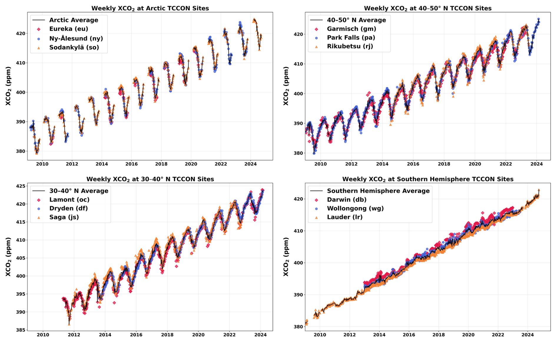
Figure A1 Time series of weekly XCO₂ measurements from selected TCCON stations and regional averages, covering the period from 2009 to 2024. Each panel corresponds to a different study region: (top left) Arctic sites, (top right) 40–50° N, (bottom left) 30–40° N, and (bottom right) Southern Hemisphere sites. Colored markers represent individual TCCON station measurements, while the black line shows the smoothed regional average, with gaps masked where data is not available.

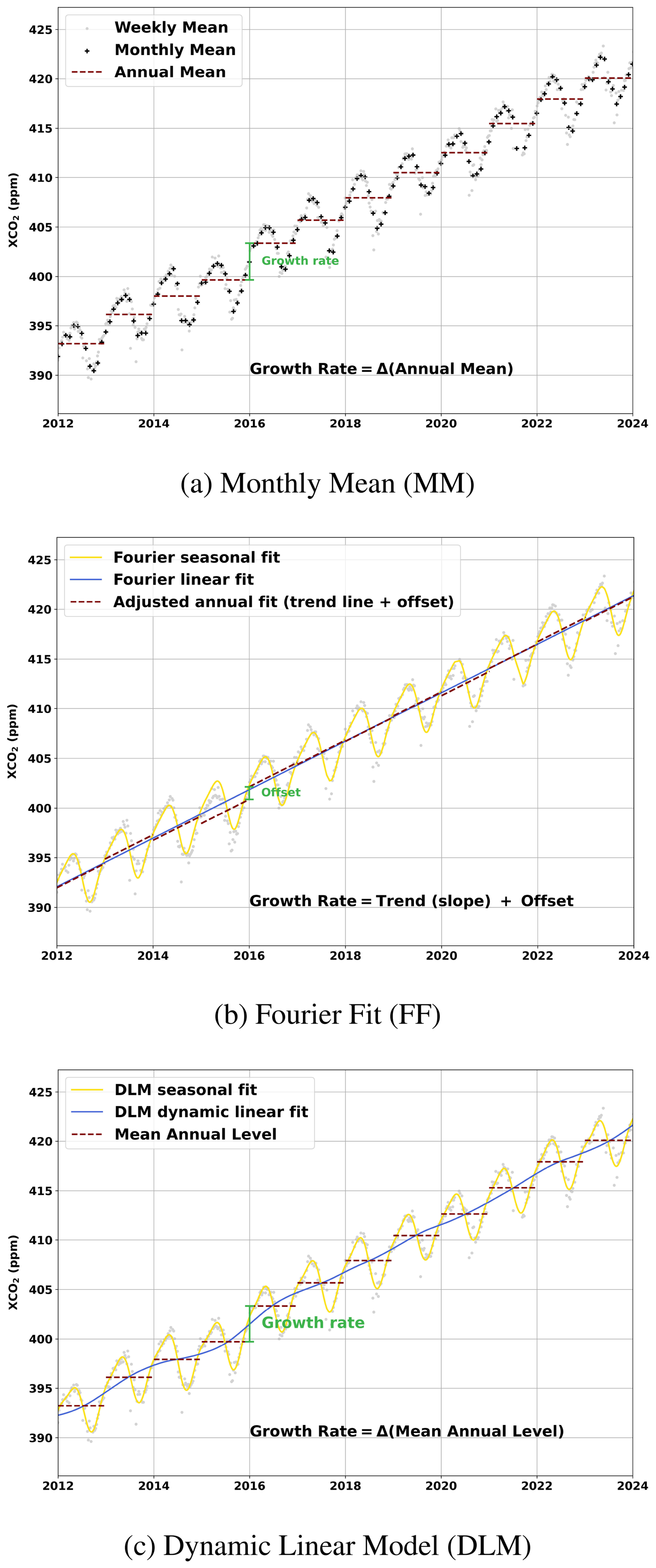
Figure A2 Illustration of the three methods used to derive annual CO₂ growth rates at Lamont TCCON station: (a) Monthly Mean (MM), (b) Fourier Fit (FF), and (c) Dynamic Linear Model (DLM). In panel (a), black crosses indicate monthly mean XCO₂ values, with dashed red lines showing annual means; the growth rate is defined as the difference between consecutive annual means (ΔAnnual  Mean). In panel (b), the blue line represents the linear trend, the yellow curve the full Fourier seasonal fit, and dashed red lines the adjusted annual fits after applying yearly offsets; the total growth rate combines the long-term trend (slope) with the offset contribution. In panel (c), the DLM decomposition is shown, where the blue line depicts the dynamic linear trend, the yellow line the seasonal component, and dashed red lines mark the mean annual levels. The green segment in each panel illustrates an example of year-to-year changes used to calculate the corresponding growth rates.

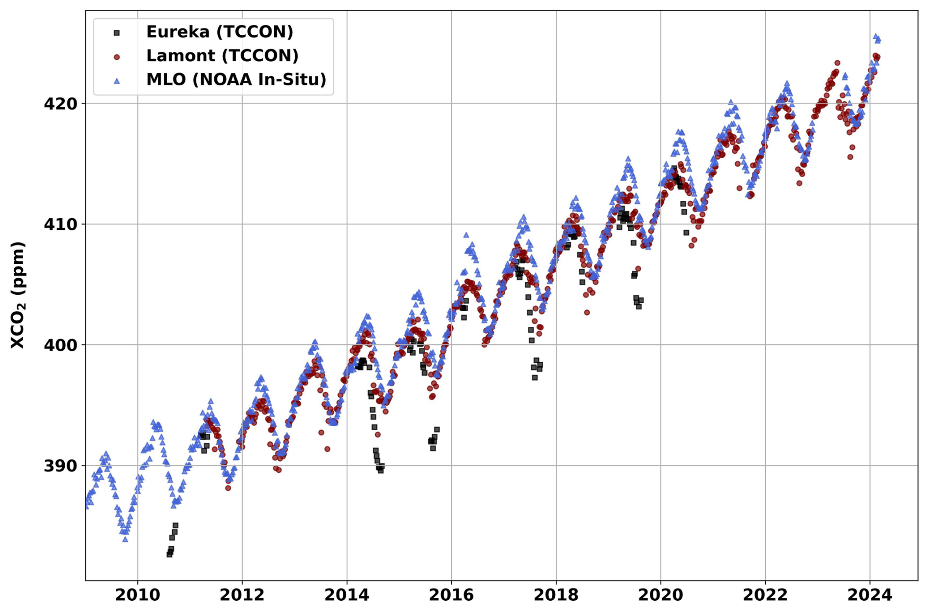
Figure A3 Time series of weekly averaged ground-level CO₂ concentrations from the NOAA MLO site and weekly averaged XCO₂ measurements from the Lamont and Eureka TCCON sites

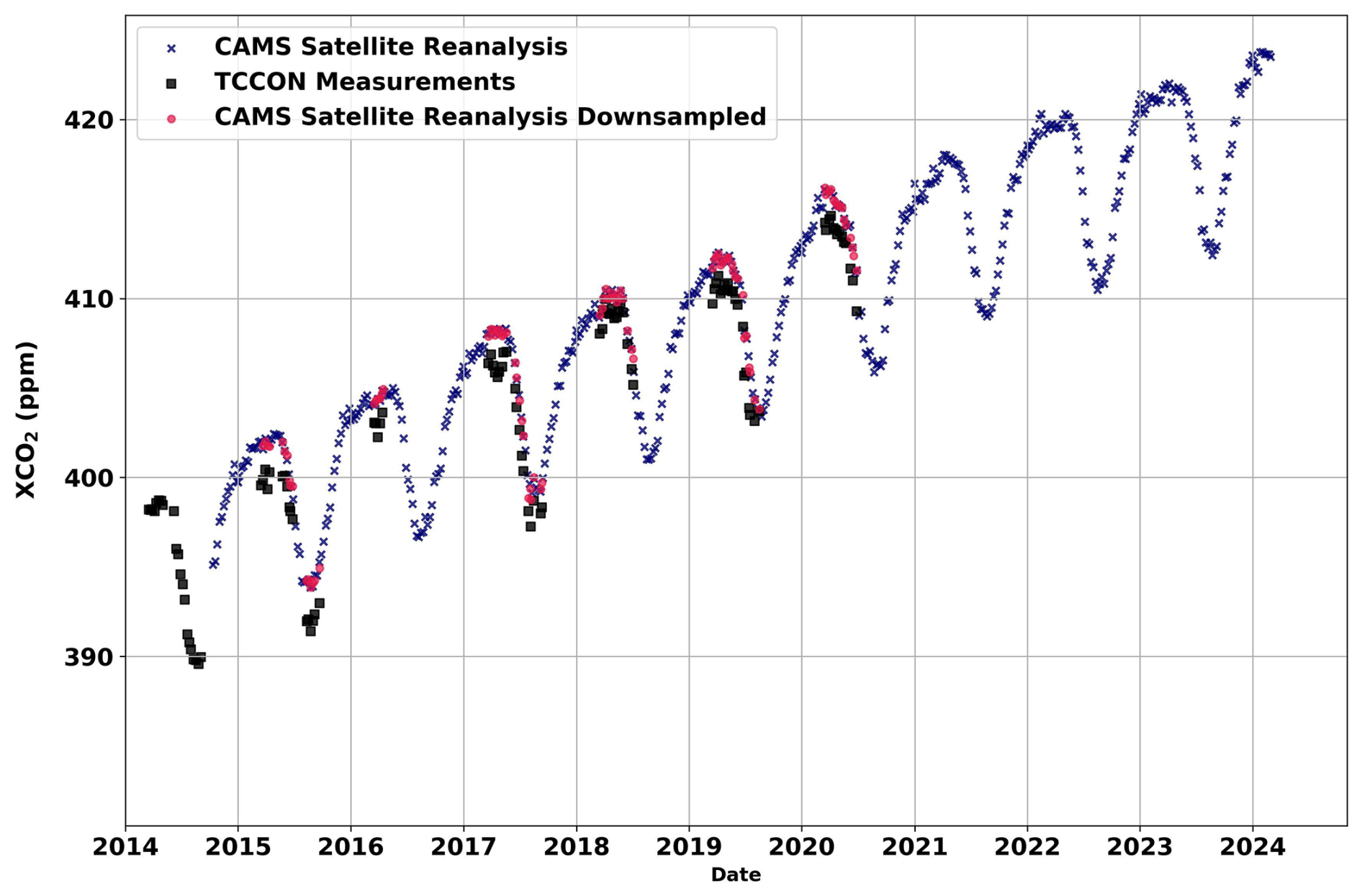
Figure A4 Time series of weekly averaged XCO₂ from the Eureka TCCON overlaid with CAMS reanalysis data from the nearest grid point to each as well as the downsampled CAMS timeseries.

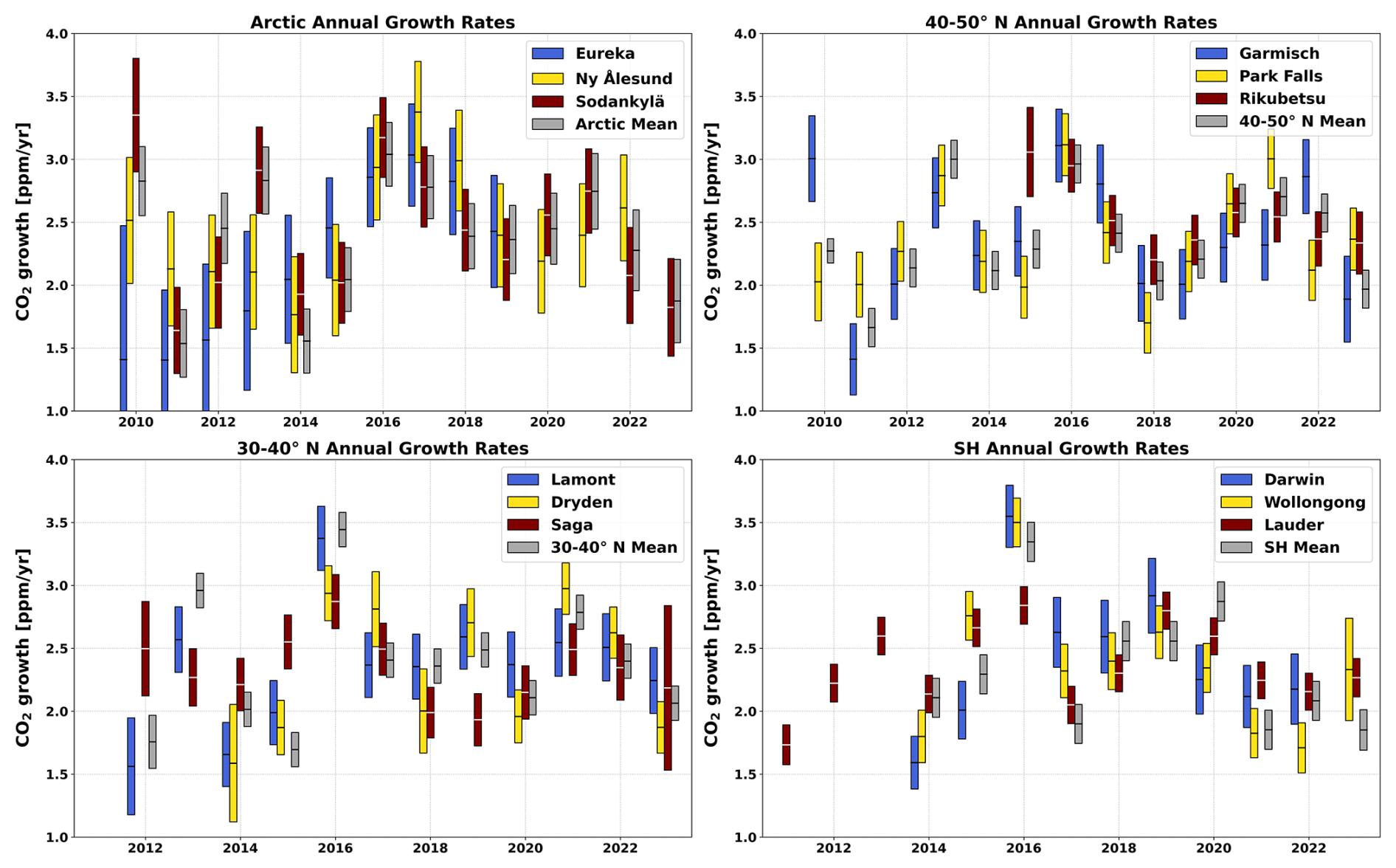
Figure A5 Annual CO₂ growth rates derived from TCCON stations, covering 2009–2024. Each panel corresponds to a different study region: (top left) Arctic sites, (top right) 40–50° N, (bottom left) 30–40° N, and (bottom right) Southern Hemisphere sites. Colored bars show annual growth rates for individual stations, and grey bars indicate the average of all sites within the region. The central line within each bar indicates the median growth rate, and the bar length reflects the associated uncertainty.

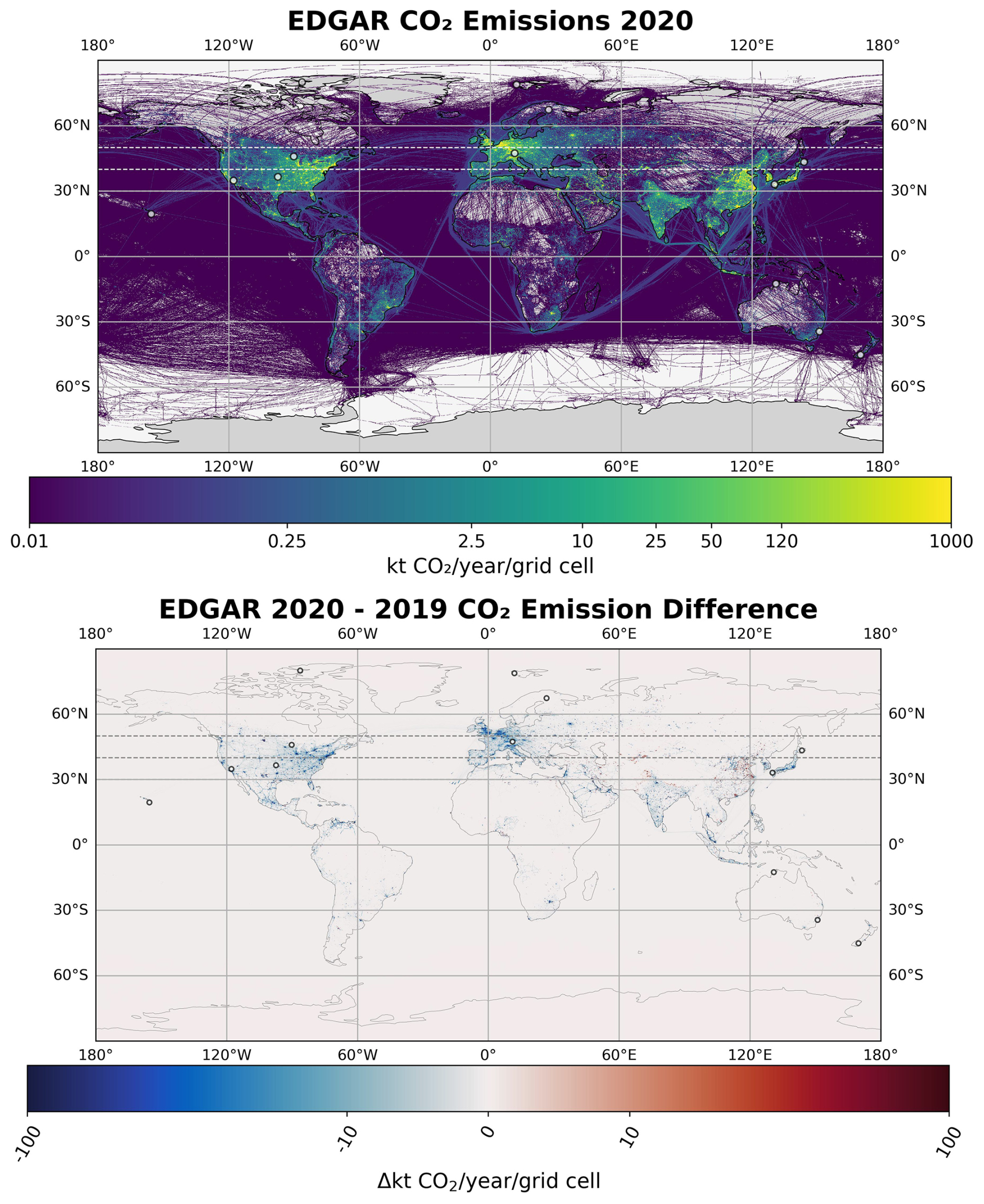
Figure A6 Top: Map of 2020 fossil fuel emissions based on the EDGAR 2020 fossil fuel flux data, displayed at a 0.1° × 0.1° resolution (Crippa et al., 2023). Bottom: Map showing the difference in emissions between 2020 and 2019 at the same resolution. The locations of TCCON stations used in this study are marked with yellow circles, while additional horizontal lines at 40 and 50° N are added to indicate the latitude bands used for regional analysis. Global map based on Natural Earth public domain data and plotted using the Cartopy Python library (Met Office, 2024; Natural Earth, 2025).