Alternative dynamic regimes of marine biogeochemical models in perturbed environments

The existence of alternative dynamic regimes or equilibria has been widely observed in the biosphere and the climate system. In order to assess the potential impacts of climate change and develop effective mitigation and adaptation strategies, a comprehensive knowledge of these alternative regimes is crucial. We studied marine biogeochemical cycles, which are fundamental for sustaining ocean life and for climate regulation, with a state-of-the-art biogeochemical model. We investigated whether the perturbation of the environment (e.g. air temperature, wind velocity, nutrient input) to extreme values can push biogeochemical cycles into a different regime. We have established that alternative regimes exist and that the biogeochemical cycles commonly respond reversibly to the perturbation of the environment, i.e. when the perturbation is removed the original regime is recovered. A single forcing, depletion of nutrients, induced hysteresis in the dynamic regimes associated with changes in the planktonic trophic web, which sustains the biogeochemical cycles. The large number of numerical simulations, with a 1D water-column physical-biogeochemical model, under a vast range of environments and methodologies (sequential simulations, initial condition perturbation and demographic stochasticity) underpins the generality of the results and the sensitivity analysis of the model parameters confirms the accuracy of the model even under extreme environments. The occurrence of alternative dynamic regimes permitted us to identify possible dangerous path of the ocean state under the future climate, such as the hysteretical response under the changes of nutrient influx.

1 Introduction

Ecosystems exhibit characteristic dynamics shaped by internal processes that tend to drive them toward a theoretical equilibrium (Scheffer et al., 2001). However, human activities and anthropogenic climate change are altering these dynamics, pushing ecosystems into alternative states. A well-documented example is coral reefs, which may shift from coral-dominated to algal-dominated systems (Mumby et al., 2007; Norström et al., 2009; Schmitt et al., 2019). When alternative (two or more) equilibrium states exist, such shifts can occur, often with profound ecological and social consequences. These transitions can be difficult to reverse and hard to predict (Scheffer et al., 2001; Scheffer and Carpenter, 2003; Beisner et al., 2003; Schmitt et al., 2019; Suding et al., 2004).

Identifying stable states in nature is particularly challenging due to the inherent heterogeneity and stochasticity of ecological systems, which fluctuate over time as a result of complex interactions among their components (Sánchez-Pinillos et al., 2023). For this reason, Scheffer et al. (2001) suggested focusing on dynamic regimes rather than stable states. A dynamic regime refers to the characteristic dynamics of an ecosystem under specific environmental conditions and in the absence of major perturbations. For example, in ocean biogeochemical cycles, chlorophyll concentration can be considered a state variable: the intensity of the spring chlorophyll bloom in temperate oceans represents a dynamic regime. If environmental conditions change, the bloom intensity, and consequently the dynamic regime, may also shift. Importantly, a dynamic regime is stable under unperturbed environmental conditions but is not stationary (e.g. the chlorophyll bloom occurs only during a limited period of the year). Examples of alternative dynamic regimes have been found in aquatic and terrestrial ecosystems (Donovan et al., 2018; Lindegren et al., 2012; Hewitt and Thrush, 2010; Petraitis, 2013; Schooler et al., 2011; Schröder et al., 2005; Suding et al., 2004; Vandermeer et al., 2004) and physical systems (Van Westen et al., 2024; Wendt et al., 2024), but marine biogeochemical cycles are still poorly investigated in this context, with the exception of plankton communities (Bode, 2024; Kléparski et al., 2024; Molinero et al., 2013; Phlips et al., 2021; Soulié et al., 2022).

Biogeochemical cycles refer to the natural pathways through which essential elements and compounds circulate between living organisms and the physical environment. These cycles, including the carbon, nitrogen and phosphorus cycles, are fundamental to the maintenance of life on Earth as they regulate the availability of nutrients necessary for biological processes (Falkowski et al., 1998). Ocean biogeochemical cycles contribute to mitigating the climate crisis by absorbing carbon dioxide from the atmosphere (Falkowski et al., 1998). A fundamental role is played by plankton, which act as mediators of these processes and are responsible for half of the Earth's oxygen production (Naselli-Flores and Padisák, 2023). Due to difficulties in field observation in the marine environment, marine biogeochemical cycles are also studied using numerical models that simulate interactions among plankton communities and nutrient cycles (Fennel et al., 2022). These models offer valuable insights into the state, variability, and long-term trends of marine ecosystems, supporting scientific research and policy decisions. Their importance is underscored by their integration into major initiatives such as the European Copernicus Marine Service (CMS) and the Coupled Model Intercomparison Project Phase 6 (CMIP6; Eyring et al., 2016). Anthropogenic and natural climate change has already led to a shift in the dynamic regimes of marine ecosystems (Knowlton, 1992; Hare and Mantua, 2000; Möllmann and Diekmann, 2012). It is therefore imperative to assess whether modern biogeochemical models are able to predict alternative dynamic regimes and to identify which factors may cause a regime shift.

We assessed the occurrence of alternative dynamic regimes in the biogeochemical flux model (BFM; Vichi et al., 2020), which is used for operational purposes under the European initiative (CMS; Salon et al., 2019), i.e. to assess past, current and short-term (days to months) forecast of ocean ecosystem state. We investigated, as dynamic regimes, the seasonal properties of the planktonic ecosystem (chlorophyll bloom and deep chlorophyll maximum) and biogeochemical functions (e.g. total production of chlorophyll and nutrient recycling). A large range of environmental forcing intensities has been applied to push the set of biogeochemical cycles, hereafter referred to as the system, into alternative regimes. Since climate change is exacerbating extreme events (Gruber et al., 2021), the model was run under extreme values for the external forcings to assess the impact on alternative regimes. Particular attention has been given to whether the response of the system to the perturbation of the environmental conditions is reversible or hysteresis occurs. The conservation of ecosystems need knowledge on hysteresis because it can limit the ability to recover a desired state (Carpenter et al., 1999; Gladstone-Gallagher et al., 2024; Guarini and Coston-Guarini, 2024; Van De Leemput et al., 2016). The occurrence of alternative dynamic regimes, reversibility and hysteresis was assessed using three methods: (i) a sequence of simulations with increasing and then decreasing external forcings; (ii) an ensemble of simulations with increasing external forcing, where an ensemble of initial conditions was run for each forcing value; (iii) an ensemble of simulations with increasing external forcing, with demographic stochasticity implemented in the model. Demographic stochasticity origins from the uncertainty in birth and death events (Lindo et al., 2023; Melbourne, 2012) and may push a system to alternative regimes (DeMalach et al., 2021). These idealized numerical experiments are intended to reveal the fundamental, non-linear properties and potential thresholds inherent in the modeled biogeochemical system. The identification of alternative regimes and hysteresis under constant conditions provides crucial insight into which environmental drivers have the capacity to push the system into a different, potentially persistent state. This knowledge of the system's vulnerabilities is a critical first step in understanding how it may respond to stochastic extreme events and long-term trends, which characterize the real ocean.

This is the first time, to our knowledge, that alternative dynamic regimes have been comprehensively studied in biogeochemical models. We have investigated more than 4000 possible scenarios, taking into account each dynamic regime, the magnitude of the forcings and the numerical experiments, in order to obtain general results suggesting under which environmental forcing alternative dynamic regimes exist and whether the system is reversible or hysteresis occurs. The ability to run simulations over a period of 100 years also confirmed that the regimes are not transient, which is a risk when short-term observations are used to identify alternative dynamic regimes (Schröder et al., 2005).

2 Methods

2.1 Biogeochemical model

Plankton dynamics and biogeochemical cycles in a 1-D water column are produced by the coupling between the Biogeochemical Flux Model (BFM) (Vichi et al., 2020) and the General Ocean Turbulence Model (GOTM) (Burchard and Petersen, 1999). This model configuration is described in detail in Álvarez et al. (2023) and in the BFM code manual (Vichi et al., 2020). Here we give a brief overview of the model, focusing on the plankton dynamics, and a more detailed overview is provided in the Supplement.

The biogeochemical flux model (BFM) consists of a system of N_tot=54 ordinary differential equations describing the cycling of carbon, phosphorus, nitrogen, ammonium, silica and oxygen through inorganic, living, dissolved and particulate organic phases. The transmission of light in the water column is resolved in 33 wavebands centered on wavelengths ranging from 250 to 3700 nm (Lazzari et al., 2021b), with the light being absorbed and scattered by the water, phytoplankton, chromophoric dissolved organic matter (CDOM) and detritus (Álvarez et al., 2023). GOTM, which applies vertical mixing to the BFM variables, can describe a one-dimensional water column representing saline, thermal and turbulence dynamics. BFM and GOTM are combined at runtime using the Framework for Aquatic Biogeochemical Models (FABM) (Bruggeman and Bolding, 2023). Since the computational resources required for a 1-D simulation are much smaller than for a global 3-D model, we were able to perform a large number of long simulations, but the horizontal gradients at the application sites must be either negligible or parameterized to properly describe reality.

The BFM describes the lower trophic level of marine ecosystems with primary producers (phytoplankton), predators (zooplankton) and decomposers (bacteria). These groups are then subdivided into plankton functional types (PFTs), which differ in their ecological function. Phytoplankton are subdivided into diatoms (P1), nanoflagellates (P2), picophytoplankton (P3) and dinoflagellates (P4). Zooplankton in nanoflagellates (Z6), microzooplankton (Z5), omnivorous mesozooplankton (Z4) and carnivorous mesozooplankton (Z3). Bacteria (B1) are represented by a single PFT and are responsible for the fundamental aspect of recycling organic compounds into inorganic constituents such as nitrate, phosphate and silicates. The growth of primary producers is limited by nutrients (phosphate, nitrate and ammonium), light and temperature; diatoms also require silicate to form a protective shell. In the original version of the BFM, the rate of metabolic processes increases monotonically with the water temperature (Lazzari et al., 2021a). We have adopted the more realistic description of Blackford et al. (2004) so that the rate of these processes increases with temperature up to a threshold (32 °C), after which the rate slowly decreases, representing enzyme degradation at high temperatures (see Eq. S4 in the Supplement). The grazing of phytoplankton by zooplankton is described by a Holling type II functional response (Gentleman et al., 2003). Both phytoplankton and zooplankton release CO₂ by respiration and organic matter by excretion. The main function of bacteria is the remineralization of particulate detritus and dissolved organic matter, but they can also act as competitors to phytoplankton by taking up inorganic nutrients from the water, depending on their internal nutrient quota.

The coupled GOTM-BFM model requires atmospheric and biogeochemical forcing. We have implemented the model at the site Bouée pour l'acquisition de Séries Optiques à Long Term (BOUSSOLE) with the 1-D water column setup described in (Álvarez et al., 2023). Atmospheric forcing is provided by the ECMWF ERA5 dataset, spectral light composition at the sea surface by the OASIM model (Lazzari et al., 2021b) and temperature, salinity and biogeochemical variables come from the reanalysis of the biogeochemistry of the Mediterranean Sea (Cossarini et al., 2021). We prevented the possible occurrence of unphysical drifts during long simulations by including in the model, through the nudging presented in the Sect. 2.3, a relaxation effect of the following variables to observational data: temperature, salinity, phosphate, nitrate, oxygen, alkalinity, dissolved inorganic carbon. The relaxation time is very long in order to minimize the effects on seasonal timescale on which response indicators are considered. The model was numerically integrated with climatological-averaged forcings from 2000 to 2050 with a time step of 10 min, and the day-to-day averages of the last 5 years of the model output were stored.

The BOUSSOLE site is located in the Ligurian Sea over deep waters (2350–2500 m), where currents are extremely weak due to its position near the center of the basin's cyclonic circulation, making a 1-D configuration appropriate. The site experiences strong winter mixing, that homogenizes the water column, and a marked spring–summer stratification, which together shape its ecological response (Antoine et al., 2006). This seasonal cycle drives a shift from nutrient-rich winter conditions supporting the spring bloom to strongly oligotrophic summer surface waters, with chlorophyll concentration often <0.1 mg m⁻³ (Antoine et al., 2006). These dynamics are correctly reproduced by the model, as showed by the climatological annual distributions of chlorophyll, phosphate, nitrate, ammonium and photosynthetically active radiation PAR (see Fig. 1). These features suggest that the system is sensitive to perturbations affecting nutrient supply and mixing conditions during winter and spring and light attenuation during summer.

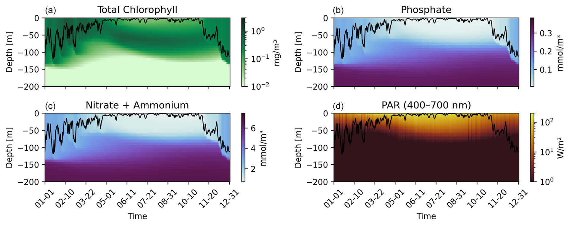
Figure 1 Hovmöller plots of oceanographic variables at the BOUSSOLE site for a climatological year, obtained from model outputs. Each panel shows the temporal evolution along the top 200 m of the water column: (a) Total Chlorophyll [mg m⁻³], (b) Phosphate [mmol m⁻³], (c) Nitrate + Ammonium [mmol m⁻³], and (d) Photosynthetically Active Radiation (PAR, 400–700 nm) [W m⁻²]. The black line in each panel represents the mixed layer depth (MLD).

2.2 Alternative dynamic regimes

We are interested in the existence of alternative stable states in our modeled ecosystems. Since real ecosystems are never stationary because natural populations always fluctuate (e.g. due to a seasonal environment), we adopt the nomenclature of Scheffer and Carpenter (2003) and indicate the “stable states” with the term “dynamic regimes”. In particular, we define a dynamic regime as the characteristic dynamics expressed by an ecosystem under given environmental conditions. By characteristic dynamics we mean a specific pattern of the system that persists over time while maintaining consistent properties. Alternative dynamic regimes occur when two or more distinct regimes can exist within the same ecosystem. In the following, the terms dynamic regime and regime are used interchangeably. Two types of alternative dynamic regimes are possible (Beisner et al., 2003): (i) coexisting regimes, where multiple regimes can exist under the same conditions and the ecosystem may shift from one to another in response to disturbances affecting the state variables; and (ii) condition-dependent regimes, where different regimes arise only under different conditions, such as changes in environmental forcings that alter the ecosystem regime.

When a parameter changes due to a perturbation, the dynamic regime of the ecosystem may change, tracing a (forward) path through the space of possible dynamic regimes. When the perturbation is relaxed (backward path) and the parameter returns to its original value, two scenarios are possible. The dynamic regime can return to its original value by following the same trajectory it followed under the perturbation (see Fig. 2, left panel), in which case the system is reversible. If the regime moves along a different trajectory (see Fig. 2, right panel), the system exhibits hysteresis (Beisner et al., 2003), which can only occur if alternative dynamic regimes exist for the same value of the parameter. After hysteresis, it may be more difficult or even impossible for the system to return to its original state, which is why predicting hysteresis is fundamental for ecologists and managers.

A minimal model showing alternative dynamic regimes and hysteresis is the Hill model (Scheffer et al., 2001), which is a mathematical model describing an ecosystem property X under environmental forcings:

$$\begin{array}{}\text{(1)}& {\displaystyle \frac{\mathrm{d}X}{\mathrm{d}t}}=a-bX+rf\left(X\right)\end{array}$$

where a is an environmental condition that promotes X, b is the rate of decay of X, r is the rate at which X recovers, where

$$\begin{array}{}\text{(2)}& f\left(X\right)={\displaystyle \frac{X^p}{X^p+h^p}}.\end{array}$$

f(X) is a function with a threshold, called the Hill function, and p a parameter determining the steepness of the switch occurring around h. For phytoplankton, one could interpret X as biomass, a as nutrient input, b as predation and r as migration.

We are interested in the steady state value $\overline{X}$ of the state variable X, or the dynamic regime as in the BFM case, and in particular to its dependency on the model parameters p and a. For different values of p, $\overline{X}$ responds differently to perturbation of the environmental condition a. For example for p=2 (and $b=r=h=\mathrm{1}$), for each value of a there is only a corresponding $\overline{X}$, showing therefore a reversible response to the variation of a (see left panel of Fig. 2). For higher p (p≥4 and $b=r=h=\mathrm{1}$, numerically obtained), two values of $\overline{X}$ are possible for the same a, giving rise to hysteresis (see right panel of Fig. 2). In the Hill model, dynamic regimes correspond to stationary solutions of the state variable $\stackrel{\mathrm{̃}}{X}$, where $\mathrm{d}\stackrel{\mathrm{̃}}{X}/\mathrm{d}t=\mathrm{0}$. In contrast, the BFM lacks stationary solutions due to daily and seasonal forcings, and dynamic regimes are defined as state variable values at specific times and depths that characterize biogeochemical processes. For example, for the annually recurring surface chlorophyll peak, the dynamic regime is defined as the value of its intensity under the specific environmental conditions of the simulation (e.g., an annual mean air temperature of 17 °C). In the BFM, these environmental conditions are determined by the model forcings, which play the role of parameter a in the Hill model; by varying forcing magnitude, the model can visit different (alternative) dynamic regimes. To minimize numerical noise, dynamic regimes were estimated as the mean over the final five simulated years. We quantitatively discriminate alternative regimes occurring at the same environmental condition computing the coefficient of variation (CV) between the two regimes, CV>0.1 indicates different regimes and hysteresis occurred.

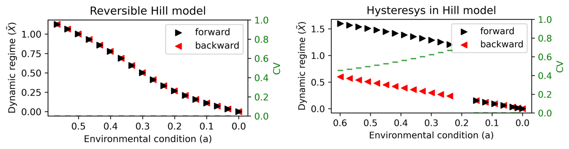
Figure 2 Bifurcation diagrams showing the response of the Hill model's dynamic regimes to the environmental condition a. The y axis value ($\stackrel{\mathrm{̃}}{X}$) is the steady state solution of the Hill model (Eq. 1). The left panel show a reversible response of the Hill model with parameters p=2 and $b=r=h=\mathrm{1}$, the forward path (black), from original to extreme environmental condition, and the backward path (red), from extreme to original environmental condition, follow the same trajectory satisfying CV<0.1. The right panel show the hysteresis in the Hill model with parameters p=18 (chosen to obtain a figure similar to the BFM outputs shown in the following) and $b=r=h=\mathrm{1}$, the forward path (black), from original to extreme environmental condition, and the backward path (red), from extreme to original environmental condition, follow different trajectories satisfying CV>0.1.

2.3 Nudging of biogeochemical variables

Relaxation of model variables through nudging is used both to prevent unphysical drifts (Sect. 2.1) and as a theoretical forcing to perturb the system (Sect. 2.4). Therefore, clarification of the nudging approach is warranted; here we use phosphate as an illustrative example. Phosphate nudging means that the variable phosphate relaxes during the simulation to a certain vertical profile with a certain relaxation time τ, i.e. at each point of the vertical grid the phosphate variable is evolved as follows

$$\begin{array}{}\text{(3)}& \begin{array}{rl}{\displaystyle \frac{\partial P}{\partial t}}(z,t)& =\left(\begin{array}{c}\text{physical}\\ \text{processes}\end{array}\right)+\left(\begin{array}{c}\text{biogeochemical}\\ \text{processes}\end{array}\right)\\ & -\left({\displaystyle \frac{P(z,t)-P_{\mathrm{nudging}}(z,t)}{\mathit{\tau }}}\right).\end{array}\end{array}$$

To prevent unphysical drift the vertical profile (P_nudging) is obtained from observations. In contrast, in our perturbation experiments the nudging acts as a forcing: the vertical profile toward which the model relaxes is systematically increased or decreased. The perturbation is applied uniformly across the vertical grid, and a relaxation timescale of τ=1 year is used, consistent with Álvarez et al. (2023). Perturbing the phosphate nudging profile in this way is analogous to varying the parameter a in the Hill model. Similar considerations apply to the nudging of the other variables.

2.4 Experiments setup

We investigated the occurrence of alternative dynamic regimes under the perturbations of 5 parameters of the coupled GOTM-BFM model, analogues to the parameter a in the Hill model, related to the environment in which the ecosystem is located, thus we refer to them as environmental forcings. These forcings were selected based on their ecological relevance: air temperature and wind as the major drivers of vertical mixing, suspended particulate matter (SPM) as the main factor limiting light availability, phosphate as a key determinant of nutrient concentrations (given that nitrogen is supplied through both nitrate and ammonium), and oxygen to capture potential hypoxia effects. The magnitude of the forcing perturbations was chosen to be large relative to the climatological mean in order to explore potential thresholds, while remaining within the range of extreme but physically plausible conditions reported in observations and paleoclimate records (Blanchard-Wrigglesworth et al., 2023; Blomquist et al., 2017; Cossarini et al., 2021; Grisogono and Belušić, 2009; Lohmann et al., 2020; Palter et al., 2005; Walbröl et al., 2024). The atmospheric forcings have a temporal dimension with seasonal variability and no inter-annual variability, the marine forcings also depend on the depth. To examine the emergence of alternative regimes under extreme environmental conditions, a constant offset was added to the forcings to modify their annual mean. Simulations were carried out under annually, repeating environmental conditions, with different simulations distinguished only by their mean forcing magnitude, while retaining identical intra-annual variability. The mean of the forcing has a role similar to the environmental condition a of the Hill model. Long periodic simulations were performed to remove transient dynamics and ensure convergence to stable dynamic regimes. The full list of studied forcings and their range of variability is given in Table 1.

We identified a list of target indicators focusing on the plankton community and biogeochemical cycles. We examined 6 indicators related to the chlorophyll bloom, 6 indicators related to the deep chlorophyll maximum (DCM), and 8 indicators related to the aggregated system production and cycling. These indicators are commonly used in studies assessing the state and sensitivity of marine biogeochemical cycles (Ciavatta et al., 2025). The full list of target indicators with the computation method is given in Table 2.

We performed 4 experiments consisting of a set of simulations, with a different protocol to reach the dynamic regime. This is done to understand if the results depend on the specific choices used to construct the experiment. For each experiment we considered all the perturbations of the 5 environmental forcings. A schematic of the simulation procedure, for each experiment, is shown in Fig. 3. Prior to the experiments, a spin-up simulation with a duration of 40 years was carried out to enable a restart in which the model had already relaxed to the dynamic regimes.

Table 1 List of the forcings. In the column “Variation of the mean” the sign “+” indicates that the annual mean is increased of the range of values between square brackets, while the sign “−” indicates that the annual mean is decreased. The range of values of the original annual means for some forcings is due to a vertical variability through the water column.

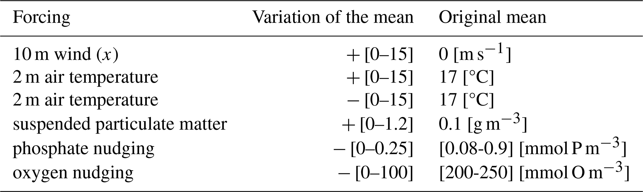
Table 2 List of the target indicators of the ecosystem studied as system response to the perturbation of parameters, divided in three major categories: CHL bloom, DCM, aggregated ecosystem production and cycling.

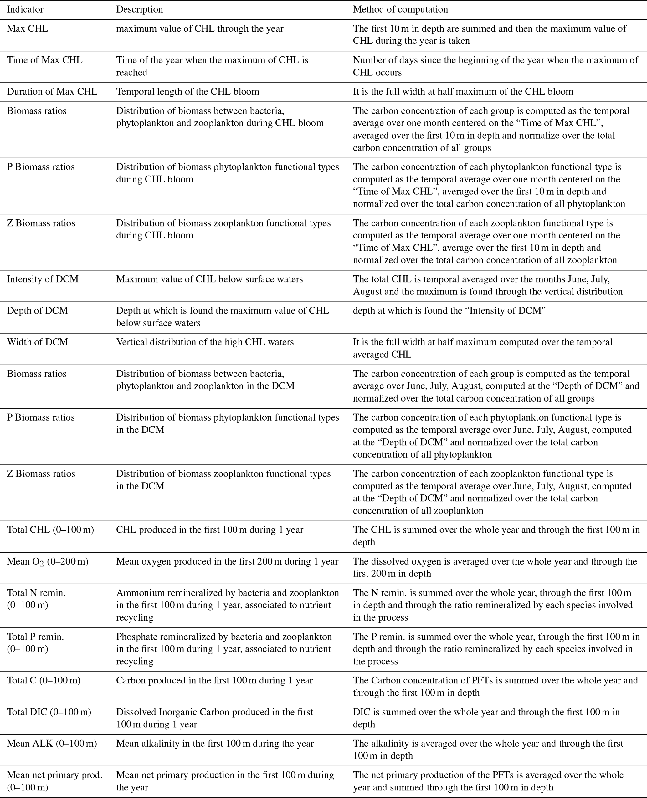
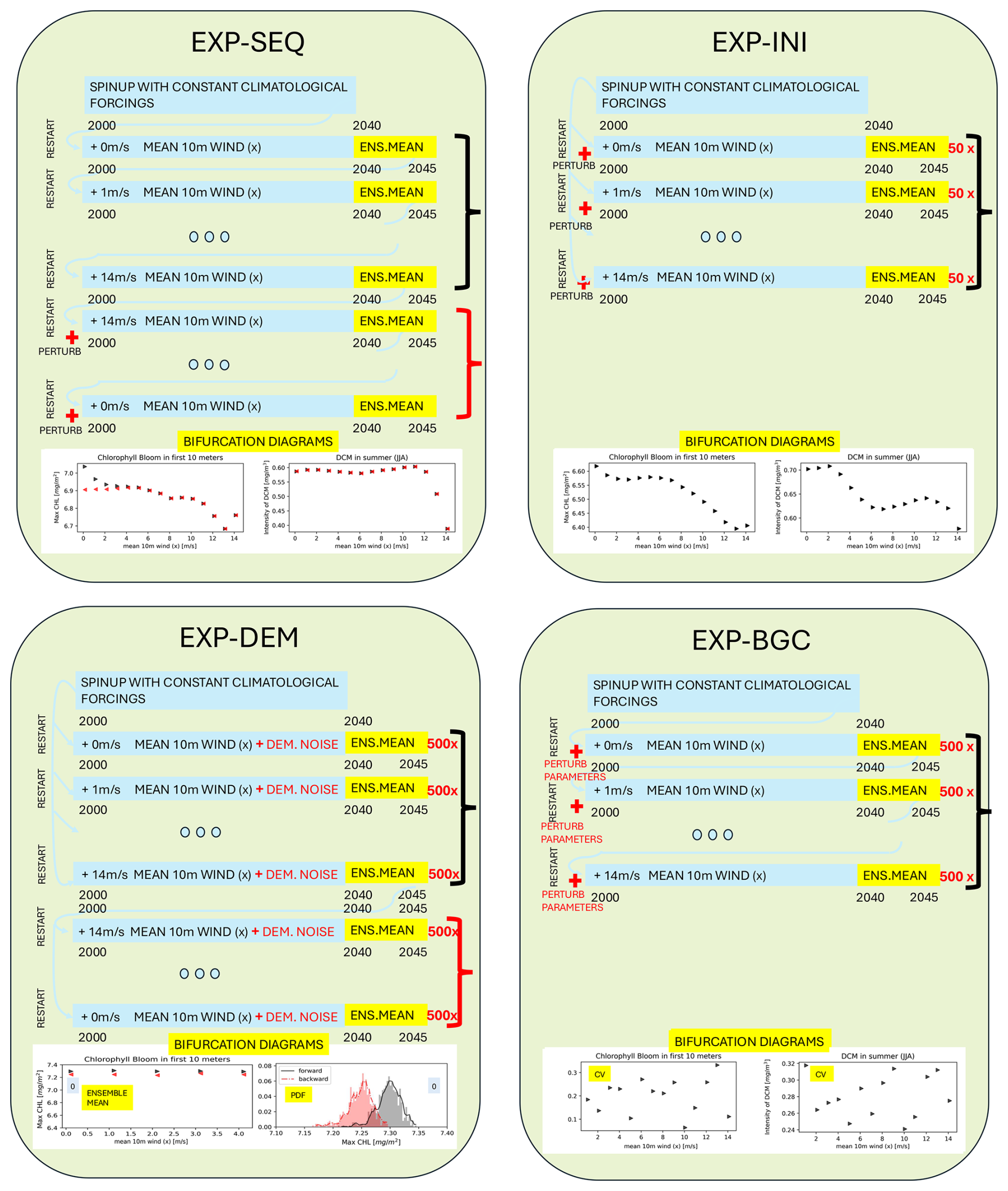
Figure 3 Protocols of the simulation experiments EXP-SEQ, EXP-INI, EXP-DEM, and EXP-BGC. The experiments methodology is described in Sect. 2.4. For each EXP we considered the effects of the perturbation of the 6 environmental forcings, listed in Table 1, over all the target indicators, listed in Table 2. Here the forcing 10 m wind (x) is taken as an example.

2.4.1 EXP-SEQ: Sequential simulations

The first experiment (EXP-SEQ) is designed to test whether the ecosystem follows the same path when an environmental forcing is gradually intensified as when it is gradually relaxed, i.e. whether the system is reversible or whether it exhibits hysteresis. To address this question, two sets of 15 sequential simulations with a length of 45 years were carried out for each forcing: in the first set of simulations, i.e. forward simulations, the mean value of the forcing was increased (decreased); the second set, i.e. backward simulations, restarts from the end of the first set and the mean value is decreased (increased), in this set the concentration of living species is perturbed at the beginning of the simulation. The perturbation prevents extinction and allows to observe new alternative regimes with respect to the forward simulations. The PFTs concentration is characterized by three intra-cellular quota element (C, N, P). The perturbation is applied to these quota as follows: $+{\mathrm{10}}^{-\mathrm{2}}$ C for carbon, $+{\mathrm{10}}^{-\mathrm{4}}$ N for nitrogen and $+{\mathrm{10}}^{-\mathrm{5}}$ P for phosphorus, equally for each species. This perturbation represents a demographic variability, always present in natural populations which is not described by the model and can prevent extinction. The day-to-day mean of the last 5 years of each simulation is stored. The dynamic regimes are computed for each simulation and plotted in a bifurcation diagram (similarly to Fig. 2) to determine whether the system is reversible or hysteresis occurs. The sequence of simulations is repeated separately for each forcing.

2.4.2 EXP-INI: Random initial condition simulations

Alternative dynamic regimes may, in theory, be associated with specific initial conditions. As a result, EXP-SEQ could potentially overlook these regimes. The second experiment (EXP-INI) aims to determine whether the model can reach different dynamic regimes purely as a result of varying the initial conditions, and to assess how this sensitivity depends on the magnitude of the environmental forcings. To explore this, for each magnitude of the investigated forcing, e.g. for a mean 10 m wind (wind at 10 m above the sea surface), we performed an ensemble of 50 simulations with different initial conditions: (i) for carbon and nutrients of the plankton species, a random value ranging ±70 % from the restart value provided by the spinup simulation with climatological forcings; (ii) for the remaining variables, the restart of the spinup simulation. The simulation ensembles are then used to generate bifurcation diagrams, which allows to observe whether alternative dynamical regimes exist simultaneously for the same magnitude of environmental forcings. The simulations ensemble is repeated separately for each forcing.

2.4.3 EXP-DEM: Demographic noise simulations

The third experiment (EXP-DEM) investigates whether random fluctuations in the plankton populations, inherent in realistic ecosystems, can drive the system from one dynamic regime to another, and how this sensitivity depends on the magnitude of the environmental forcings. If there are alternative dynamic regimes, a stochastic perturbation can push the system into the region of attraction of another dynamic regime. In this experiment, we incorporated the stochasticity of birth and death events, which are assumed to be independent between individuals, like the demographic noise in the biogeochemical model. This effect can be represented by a multiplicative white noise acting on the biomass of the plankton species with a sublinear scaling with respect to the biomass (Arnoldi et al., 2019). In the BFM, we applied the noise to the biomasses of bacteria, phytoplankton and zooplankton. The biomass Xⁱ of a general PFT is evolved by the following stochastic differential equation

$$\begin{array}{}\text{(4)}& \mathrm{d}{X}^i={\text{BFM}}_{X^i}(\mathit{X},t)\mathrm{d}t+D^i{k}^i\sqrt{X^i}\mathrm{d}W,\end{array}$$

where ${\text{BFM}}_{X^i}$ denotes the deterministic dynamics of the biomass Xⁱ provided by the deterministic version of the BFM, X is the vector of the N_tot state variables, W is a Wiener process and $k^i=\sqrt{\mathrm{1}\mathrm{mg}\mathrm{C}{\mathrm{m}}^{-\mathrm{3}}}$ is a normalization factor. We studied three noise intensities $D^i=[\mathrm{0.01},\mathrm{0.001},\mathrm{0.0001}]d^{-\mathrm{1}/\mathrm{2}}$, equal for each PFT. For each magnitude of the investigated forcing we performed an ensemble of 500 stochastic simulations from which we computed an averaged dynamic regime, used to generate bifurcation diagrams, and the probability distribution function (PDF) of the regime. The simulation ensemble is repeated separately for each forcing. We performed two set of simulations one using as initial conditions the restart of the spinup simulation (forward simulations), another using as initial condition the ensemble mean of the restarts of the forward simulation with the largest environmental forcing (backward simulations). These two sets are compared similarly as done in the experiment EXP-SEQ.

2.4.4 EXP-BGC: Biogeochemical parameters sensitivity analysis

The fourth experiment (EXP-BGC) aims to assess whether the dynamic regimes identified by the model are sensitive to the parametrization of the biogeochemical model (BFM), and to what extent, with the ultimate goal of constraining the uncertainty of the findings. To this end, we perturbed 10 key parameters governing plankton dynamics, selected from those identified as most influential in the SEAMLESS project (Ciavatta et al., 2022), based on a global sensitivity analysis of the model. For the 4 phytoplankton PFTs, we perturbed 2 parameters regulating primary productivity: the maximum specific productivity ($p\mathit{\_}\mathrm{sum}\in [\mathrm{1.25},\mathrm{4.75}]{\mathrm{d}}^{-\mathrm{1}}$) and the reference ratio Chl:C ($p\mathit{\_}\mathrm{qlcPPY}\in [\mathrm{0.005},\mathrm{0.038}]\mathrm{mg}\mathrm{Chl}\mathrm{mg}{\mathrm{C}}^{-\mathrm{1}}$). For the microzooplankton, characterizing the plankton dynamics being in the center of the modeled food web (Occhipinti et al., 2023), we perturbed two parameters regulating its growth: the assimilation efficiency ($p\mathit{\_}\mathrm{pu}\in [\mathrm{0.35},\mathrm{0.65}]$) and the fraction of activity excretion ($p\mathit{\_}\mathrm{pu}\mathrm{\_}\mathrm{ea}\in [\mathrm{0.35},\mathrm{0.65}]$). For each magnitude of the forcing studied we performed an ensemble of N_ens=500 simulations with different parameters. The simulation ensemble is repeated separately for each forcing. The simulation ensembles are then used to compute the coefficient of variation (CV) of the dynamic regimes at each magnitude of the environmental forcings, with the aim of investigating a relationship with the parameter uncertainty and the strength of the forcings. The CV is computed for a dynamic regime χ over the simulation ensemble as

$$\begin{array}{}\text{(5)}& {\text{CV}}_{\mathit{\chi }}={\displaystyle \frac{{\mathit{\mu }}_{\mathit{\chi }}}{{\mathit{\sigma }}_{\mathit{\chi }}}}={\displaystyle \frac{{\sum }_{\mathit{\alpha }=\mathrm{1}}^{N_{\mathrm{ens}}}{\mathit{\chi }}_{\mathit{\alpha }}/N_{\mathrm{ens}}}{\sqrt{{\sum }_{\mathit{\alpha }=\mathrm{1}}^{N_{\mathrm{ens}}}({\mathit{\chi }}_{\mathit{\alpha }}-{\mathit{\mu }}_{\mathit{\chi }}{)}^{\mathrm{2}}/N_{\mathrm{ens}}}}},\end{array}$$

where μ_χ and σ_χ are, respectively, the mean and standard deviation of the dynamic regime χ over the ensemble of simulations, numbered $\mathit{\alpha }=\mathrm{1},\mathrm{\dots },N_{\mathrm{ens}}$, and χ_α is the dynamic regime computed for the simulation α.

3 Results

3.1 EXP-SEQ

In the experiment performing sequential simulations under variation of environmental forcing (EXP-SEQ), we found both reversibility and hysteretic response of the system. We present the results related to the forcings associated to reversible response in Fig. 4 and associated to hysteresis in Fig. 5.

We observe reversible response in many experiments, the model visits alternative dynamic regimes under the variation of wind, air temperature (airt), suspended particulate matter (spm) and oxygen (oxy), not shown, among those of Table 2. The visited regimes are the same (differences satisfy CV<0.1) in the forward path, where the forcing increases, and in the backward path, where the forcing decreases (see Fig. 4). The system is, thus, reversible under these forcings because the dynamic regime can return to its original value (the first value on the left in each plot) by following the same trajectory it followed under the perturbation.

The model showed the presence of hysteresis under the variation of phosphate nudging. The system never returns to the dynamic regime it was in before the perturbation of the environmental forcings. The forward path, from original to extreme environmental forcing, and the backward path, from extreme to original environmental forcing, follows different trajectories. Under phosphate nudging perturbation the hysteresis is evident for all the indicators presented in Table 2 (see Figs. 5, S5 and S6). The results, confirmed by additional simulations over a period of 100 years (not shows), indicate therefore that hysteresis is not a transitory phenomenon.

We show how the plankton community is impacted by the perturbation of the environmental forcing, in the bottom panels of Figs. 4 and 5. The hysteresis under the perturbation of phosphate nudging is related to a change in the composition of the trophic web. In the backward trajectory fewer species are present in the community, in particular one phytoplankton functional type (picophytoplankton – P3 –) and two zooplankton functional types (het. nanoflagellates – Z6 – and microzooplankton – Z5 –; omnivorous mesozooplankton – Z4 – recovers only for the smallest values of nutrient depletion). In contrast, the other forcings are able to induce only reversible changes in the community composition, e.g. air temperature warming reduce the relative biomass of phytoplankton with respect to zooplankton and bacteria during the surface chlorophyll bloom.

In the Supplement, Figs. S1–S8, we show the response of all the target indicators presented in Table 2. Oxygen nudging has no strong difference in dynamic regimes and is not shown. Furthermore, we found that the decrease in air temperature has an effect similar to the increase in wind on the indicators, which is related to an increase in the mixing of the water column at lower temperature or stronger wind, therefore it is not shown.

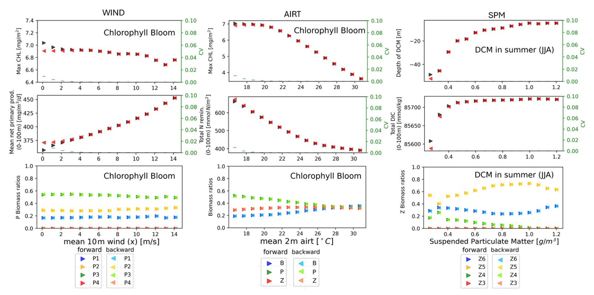
Figure 4 EXP-SEQ setup: Bifurcation diagrams showing the reversible response of the model's dynamic regimes associated to seasonal properties (top row), annual production and cycling (mid row) and community composition (bottom row) to wind (left column), air temperature (mid column) and SPM (right column). The mean magnitude of the environmental forcings (x axis) goes from its original value (left) to extreme values (right). The panels show a reversible response: the forward path (black), from original to extreme environmental condition, and the backward path (red), from extreme to original environmental condition, follow the same trajectory. For community composition (bottom row) the forward path, from original values to extreme values, is showed in darker colours and the backward path, from extreme values to original values, is showed in lighter colours. Different colours indicates different plankton groups (mid panel) or plankton functional types (left and right panels). The reversibility has been quantified with CV<0.1, shown in green. The methodology is presented in Sect. 2.4.1.

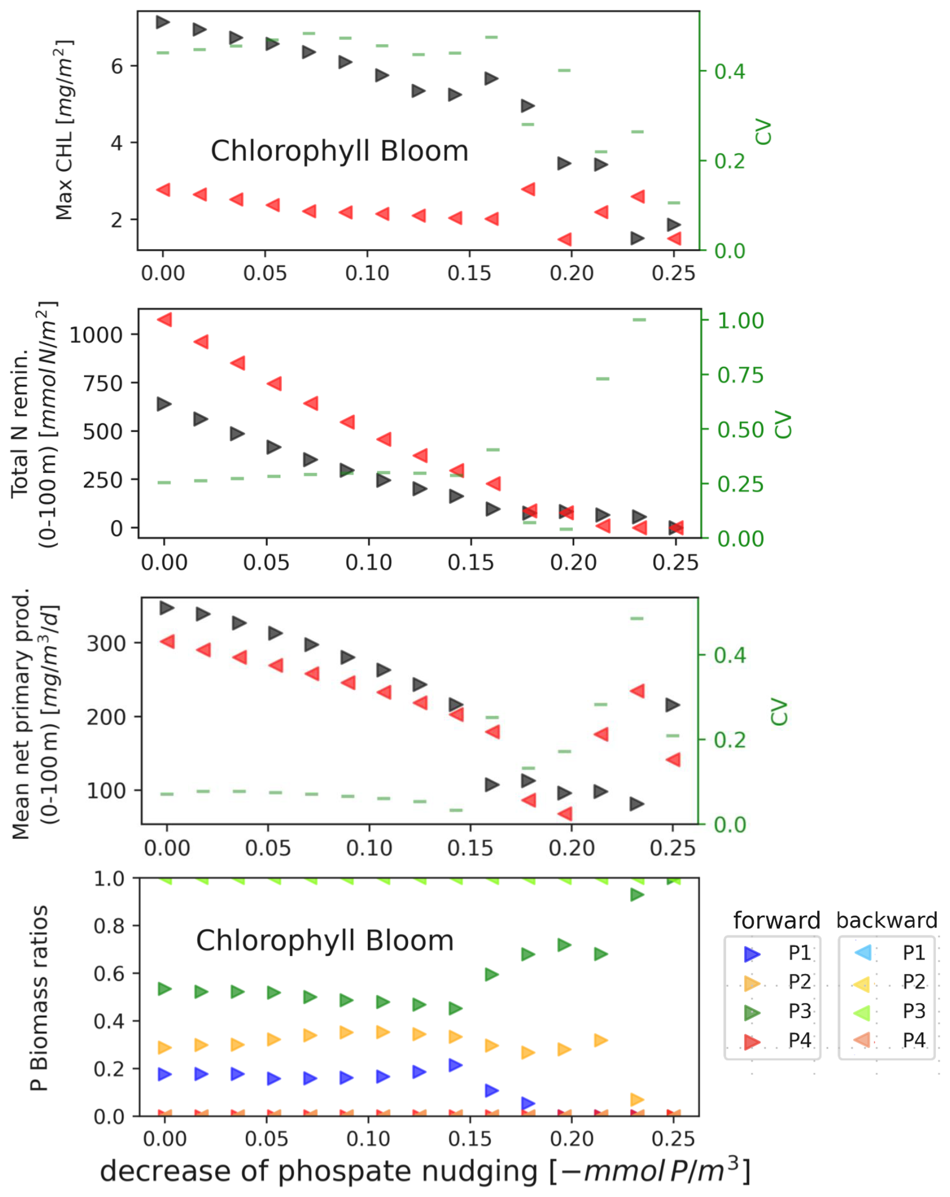
Figure 5 EXP-SEQ setup: Bifurcation diagrams showing the hysteretical response of the model's dynamic regimes associated to seasonal properties (top row), cycling (second row), annual production (third row) and community composition (bottom row) to phosphate nudging. The mean magnitude of the environmental forcings (x axis) goes from its original value (left) to extreme values (right). The panels show the hysteresis, the forward path (black), from original to extreme environmental condition, and the backward path (red), from extreme to original environmental condition, follow different trajectories. The forward path, from original values to extreme values, is showed in darker colours. For community composition (bottom row) the forward path, from original values to extreme values, is showed in darker colours and the backward path, from extreme values to original values, is showed in lighter colours. Different colours indicates different phytoplankton functional types. In the backward simulations only P3 (in green) is present. The hysteresis has been quantified with CV>0.1, shown in green. The methodology is presented in Sect. 2.4.1.

3.2 EXP-INI

Carrying out numerical simulations with random initial conditions on PFTs, under variation of environmental forcing (EXP-INI), we found that the system has, in all the cases, reversible response (see Fig. 6). As all indicators in Table 2 responded similarly to the forcings in Table 1, we show only a few representative examples. While in EXP-SEQ hysteresis was associated with strongly different alternative regimes in how the biomass is subdivided between plankton types (see Fig. 5, bottom panel), in EXP-INI no alternative regimes are found for the same magnitude of environmental forcing, not even in biomass ratios between PFTs (compare Figs. S5 and S9, bottom three panels of both columns, see Supplement).

The difference between the results of EXP-SEQ and EXP-INI is related to the fact that in EXP-SEQ we used as initial conditions the end of the previous simulation in the sequence of simulations, e.g. the initial conditions of the forward simulation with mean wind 5 m s⁻¹ were the end of the simulation with mean wind 4 m s⁻¹. In the EXP-INI experiment, only the initial conditions for carbon, phosphorus and phosphate of the plankton functional types are perturbed.

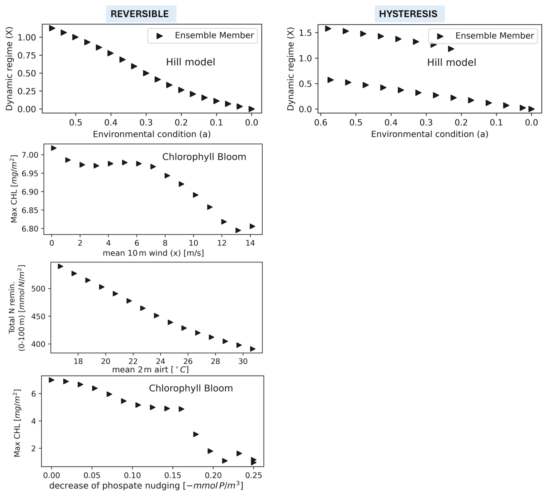
Figure 6 EXP-INI setup: Bifurcation diagrams showing the response of the model's dynamic regimes to environmental forcings. The mean magnitude of the environmental forcings (x axis) goes from its original value (left) to extreme values (right). The left panels show a reversible response: for each value of the environmental forcings all the ensemble members with different initial conditions visit the same dynamic regime (only one triangle). The right panels show the hysteresis, for some values of the environmental forcings different ensemble members visit different dynamic regimes (two triangles in column). The first row is a simplified representation of the response to environmental forcing using the Hill model (Scheffer et al., 2001), where a is a parameter of the model. The methodology is presented in Sect. 2.4.2. The other rows show the response of the dynamic regimes to the variation of 3 environmental forcings (wind, air temperature and phosphate nudging). Hysteresis never occurs for the studied forcings. CV is not shown because always smaller than 0.1.

3.3 EXP-DEM

In the experiment addressing the effect of demographic stochasticity, performing sequential simulations under variation of environmental forcing (EXP-DEM), the system presented generally a reversible response. As an example, we carried out the simulations under the variation of wind forcing (see Fig. 7), in the range of values which showed the largest difference between regimes in EXP-SEQ. Demographic stochasticity reduces the variability of dynamic regimes in response to the perturbation of the wind forcing, and the magnitude of the regimes changes less than in the deterministic experiment (EXP-SEQ), e.g. compare the first column panels in Fig. 7. The ensemble mean of the dynamic regimes is different respect to their deterministic magnitude, indicating that demographic stochasticity changes the space of possible dynamic regimes. The difference between regimes has a non-monotonic relationship with noise intensity, e.g. there is no difference in chlorophyll bloom maximum regimes for $D=\mathrm{0.001}{\mathrm{d}}^{-\mathrm{1}/\mathrm{2}}$. However the difference never overcome the threshold CV=0.01, therefore demographic noise in not able to induce hysteresis under wind forcing.

Figure 7 Bifurcation diagrams showing the response of the model's dynamic regimes to the increase of wind forcing in the EXP-DEM experimental setup. Each row shows the dynamic regimes for a different noise intensity decreasing from the top row ($D=\mathrm{0.01}{\mathrm{d}}^{-\mathrm{1}/\mathrm{2}}$) to the bottom row (deterministic solution). Along a row the first three panels show the ensemble mean of a dynamic regime for the forward (black) and backward (red) simulations. The last panel, along a row, shows the probability density function of a dynamic regime (Chlorophyll bloom Max CHL) computed over the ensemble of simulations for the first value of wind forcing (unperturbed), indicated by the “0” in the first and last panels. The methodology is presented in Sect. 2.4.3.

3.4 EXP-BGC

The dynamic regimes of the target indicators show variability in response to the perturbation of the configuration of the biogeochemical model parameters (the methodology is presented in Sect. 2.4.4), as shown in Fig. 8. The coefficient of variation (CV) of the dynamic regimes associated with seasonal patterns, chlorophyll bloom and deep chlorophyll maximum (DCM), has a CV of the order of 10⁻¹. Dynamic regimes associated with aggregated variables, e.g. total annual chlorophyll production (Total CHL), show less variability in response to parameter perturbation, with a CV of the order of 10⁻⁴.

The CV of the dynamic regimes does not show an increasing (or decreasing) trend related to the increase in wind velocity (see Fig. 8). The CV under the perturbation of the biogeochemical model parameters represents the sensitivity of the model. Therefore, the sensitivity is not affected by extreme environmental conditions. In Fig. 8 the sensitivity of the model (the dynamic regimes) under the wind forcing is shown, but similar results (no trend in CV) are obtained with the other forcings and are therefore not shown.

Figure 8 Bifurcation diagrams showing the response of the model's dynamic regimes to the perturbation of the model parameters under the increase in wind forcing (EXP-BGC, presented in Sect. 2.4.4). The y axis shows the coefficient of variation (CV) of the dynamic regimes over the ensemble of simulations with different parameters. The CV of the annual production dynamics regimes (rightmost panel) is 3 orders of magnitude lower than that of the seasonal dynamic regimes (first two panels).

4 Discussion

This study uses a comprehensive set of numerical experiments to investigate how environmental conditions affect the potential for alternative dynamic regimes and hysteresis in a complex marine biogeochemical model. The results demonstrate that such nonlinear behaviors, central to the theory of ecological regime shifts, are an emergent property of a model used for operational forecasting. By synthesizing findings across deterministic, stochastic, and sensitivity experiments, we provide a nuanced view of the primary drivers, modulating factors, and implications of these dynamics for marine ecosystems under change.

Environmental Drivers of Alternative Dynamic Regimes

Our deterministic experiments confirm that alternative dynamic regimes can arise under different environmental conditions, consistent with observational evidence of plankton regime shifts across ocean basins (Bode, 2024; Molinero et al., 2013; Reid et al., 2016). The model identifies nutrients (phosphate) as the most decisive driver, generating the most distinct alternative states. This aligns with classic limnological studies (Scheffer and Carpenter, 2003) and coastal observations where nutrient availability structures ecosystem state (Boersma et al., 2015; Peperzak and Witte, 2019). A critical finding is the hysteretic response to phosphate perturbation (Fig. 5), indicating that restoring previous nutrient levels may not reverse an ecosystem shift. This has profound management implications, as hysteresis limits recovery options (Carpenter et al., 1999; Gladstone-Gallagher et al., 2024).

Sea surface temperature is a well-documented primary driver of plankton change (Beaugrand, 2015; Soulié et al., 2022), similarly our model showed primarily reversible responses to atmospheric warming. The effects, reduced bloom intensity, deeper summer chlorophyll maxima, and lower annual productivity, are consistent with observed and projected climate impacts (Morse et al., 2017). Similarly, increased wind stress, which enhances mixing and nutrient supply, led to reversible changes in bloom phenology and increased annual production. Suspended particulate matter (SPM) is a forcing less studied in regime shift contexts. SPM increase induced clear alternative regimes (Fig. 4), primarily through light limitation, causing a shallower chlorophyll maximum and reduced diversity. This process, known as coastal darkening, is an emerging climate-related stressor (Aksnes et al., 2009). Its role is complex: SPM is increasing in high-latitude coastal waters due to glacial melt (Neder et al., 2022) but decreasing in many mid- and low-latitude regions due to human activities (Yan et al., 2025). Our results highlight SPM as a regionally variable driver capable of pushing systems between alternative states, warranting its inclusion in future assessments of ecosystem stability.

A key insight from our experiments is the prevalence of reversible system responses despite the presence of known internal feedback mechanisms within the model structure. Feedback loops, such as nutrient remineralization (Richon and Tagliabue, 2021; Stone and Berman, 1993) and light-phytoplankton interactions (Manizza et al., 2008), are recognized drivers of hysteresis and alternative stable states (Scheffer et al., 2001). Our results suggest that for most forcings (temperature, wind, SPM), these internal feedbacks are either too weak or too linear to create sufficiently deep alternative basins of attraction. Consequently, the system exhibits gradient-like, reversible change rather than catastrophic, hysteretic shifts when these drivers are altered. The singular exception is phosphate, where feedbacks related to nutrient competition, recycling efficiency, and trophic structure appear strong enough to create path dependence. This distinction between reversible and hysteretic responses is critically important. Reversible dynamics imply a greater capacity for ecosystem recovery following management intervention. In contrast, the observation of hysteresis under phosphate stress signals a fragile system, where crossing a threshold can lead to an irreversible shift to a potentially less desirable state that persists even after the original stressor is removed. For operational forecasting and ecosystem-based management, correctly diagnosing which type of response a system is prone to, reversible or hysteretic, is fundamental to setting realistic recovery targets and anticipating long-term outcomes under changing environmental pressures (Guarini and Coston-Guarini, 2024; Stecher and Baumgärtner, 2022).

4.1 The modulating roles of Initial Conditions, Stochasticity, and Model Parameters

The absence of hysteresis in the initial-condition experiment (EXP-INI) contrasts with the phosphate-driven hysteresis in EXP-SEQ. This suggests that, in this model, the long-term trajectory is more strongly governed by the external physico-chemical environment than by the initial plankton assemblage, a finding already observed in other ocean biogeochemical models (Fransner et al., 2020).

The introduction of demographic stochasticity (EXP-DEM) revealed a non-monotonic relationship between noise intensity and the separation of alternative regimes. Noise did not simply amplify or dampen differences but could either increase or decrease the distinction between states (Fig. 7). This novel finding suggests the possible occurrence of non-trivial noise-induced phenomena, as stochastic resonance (Occhipinti et al., 2024). Stochasticity also modulated the sensitivity of dynamic regimes to environmental changes (Fig. 7). We studied the effects of demographic stochasticity in the context of an increase in wind velocity, which induces an increased mixing in the water column. We may hypothesize that noise has a similar effect on mixing of plankton biomass in the water column, e.g. in the near-equilibrium limit Eq. (4) resembles the Ornstein-Uhlenbeck process (Occhipinti et al., 2024), which describes a particle moving under Brownian motion with friction (Uhlenbeck and Ornstein, 1930). Multiplicative noise may overcome wind-driven mixing because it acts along the entire water column and directly affects plankton biomass and modulate the response to wind perturbation. Overall the fact that the system responds to the variation of noise intensity similarly to the variation of wind intensity (visiting two alternative dynamic regimes) allows for the hypothesis that demographic stochasticity is not required in the considered biogeochemical model to visit different alternative dynamic regimes. On the other hand, the non-linear response of dynamic regimes suggests that some stronger phenomena can be sought in the presence of specific noise intensities.

The parameter sensitivity analysis (EXP-BGC) offers validation of the core results. The lower sensitivity of aggregated annual indicators (e.g., net primary production) compared to seasonal dynamic indicators (e.g., bloom characteristics) aligns with other model studies (Kriest et al., 2012). This underscores that the perceived stability or sensitivity of an ecosystem depends fundamentally on the chosen metrics. The model's robustness across a range of environmental perturbations supports its use in climate change studies (Reale et al., 2022). However, we emphasize that structural uncertainties (e.g., trophic complexity, functional diversity) likely exceed parametric uncertainties (Anugerahanti et al., 2020; Llort et al., 2019; Rohr et al., 2023) and could alter regime shift dynamics. For example, a more complex trophic web may include species adapted to ultra-oligotrophic conditions, which could reduce the likelihood of observing hysteresis under nutrient depletion.

4.2 Limitations and Implications for future research

Several limitations of the present study should be recognized. First, despite the model realism, simplifications remain: species diversity is represented by a limited set of PFTs, and some ecological interactions (e.g., adaptive evolution, complex life histories, or detailed benthic–pelagic coupling) are not explicitly resolved. Second, forcings were varied in idealized ways (e.g., sustained nudging or seasonally varying atmospheric drivers without inter-annual variability), so translating thresholds to real-world systems requires caution. Third, while our stochastic formulation captures demographic noise, other sources of variability (environmental stochasticity with temporal autocorrelation, spatial heterogeneity, or anthropogenic disturbances) may yield additional behaviors. Fourth, our model is applied at a specific site, and the responses to the studied perturbations may differ in other regions. For example, in high-latitude areas, future dynamics are primarily driven by stratification and sea-ice decline (Payne et al., 2025; Yamaguchi et al., 2022), so wind and temperature perturbations could elicit stronger responses and potentially induce hysteresis. In coastal upwelling regions, which are not nutrient-limited (Arroyave Gómez et al., 2021), hysteresis is therefore more likely to arise from changes in wind direction that drive upwelling, rather than from phosphate perturbations. In contrast, subtropical gyres, oligotrophic and permanently stratified regions (Dai et al., 2023), may exhibit an even stronger hysteretic response to nutrient depletion, as the absence of winter mixing prevents seasonal homogenization of the water column. Future work could address these gaps by (i) exploring structural model ensembles (multi-model or model-structure perturbation experiments) to quantify structural uncertainty; (ii) including more realistic, temporally correlated stochastic forcings (Occhipinti et al., 2025) and extreme events to test transient tipping; (iii) coupling to higher-resolution physical models to assess spatial effects on regime stability; and (iv) seeking empirical long-term observations to further validate model-inferred transitions and early-warning indicators. Additionally, developing and testing early-warning signals (Dakos et al., 2024) within the framework of complex biogeochemical models represents a vital next step for transforming the detection of alternative regimes from a diagnostic to a predictive capability.

Our results have several applied implications. First, the prevalence of reversible responses suggests that restoration and mitigation can be effective in many contexts, but the presence of hysteresis under nutrient depletion indicates situations where recovery may be slow or require stronger interventions. Second, the sensitivity of metrics to parameter uncertainty highlights the need for a careful choice of ecosystem state indicators. Third, the non-monotonic influence of demographic noise implies that stochasticity can both obscure and reveal alternative regimes, complicating early-warning signal detection but also suggesting new avenues for stochastic early-warning indicators.

A particularly concerning implication arises from the nutrient-depletion-induced hysteresis in the context of ongoing climate change. This is especially relevant for systems like the Arctic Ocean, which is projected to shift toward a more oligotrophic state, with associated changes in phytoplankton community composition and negative impacts on higher trophic levels (Oziel et al., 2017; Zhuang et al., 2021). The potential irreversibility of these transformations, as suggested by our model, further underscores the urgency of following low-emission socio-economic pathways to avoid crossing such ecological thresholds. Furthermore, the occurrence of alternative dynamic regimes in phytoplankton bloom phenology (timing, duration, intensity) raises critical questions regarding their cascading impacts on the broader marine ecosystem, given their foundational role in trophic energy transfer, CO₂ uptake, and carbon export (Nicholson et al., 2025).

5 Conclusion

This study provides the first comprehensive assessment of alternative dynamic regimes and hysteresis in a marine biogeochemical model oriented toward operational applications, bridging theoretical regime shift ecology with applied forecasting. Through an extensive set of numerical experiments, we demonstrate that the model exhibits alternative dynamic regimes under varying environmental conditions, with nutrient (phosphate) availability identified as the critical driver capable of inducing hysteresis. While most forcings (temperature, wind, SPM) elicited reversible responses, the singular case of phosphate hysteresis underscores the heightened management concern associated with nutrient-driven changes. Our results showcase that operational models possess the necessary non-linearity to simulate regime shifts, validating their use in exploring climate impacts and informing precautionary, ecosystem-based management in a changing ocean.