the Creative Commons Attribution 4.0 License.
the Creative Commons Attribution 4.0 License.
 | 27 Mar 2026
Estimation of particulate organic carbon export to the ocean from lateral degradations of tropical peatland coasts
Hiroki Kagawa
Koichi Yamamoto
Sigit Sutikno
Muhammad Haidar
Noerdin Basir
Atsushi Koyama
Ariyo Kanno
Yoshihisa Akamatsu
Motoyuki Suzuki
Peatlands serve as long-term carbon sinks and are distributed across subarctic, Arctic, and tropical regions. However, in tropical and permafrost-dominated coastal areas, coastal erosion and peat mass movement events (PMMs) have emerged as major contributors to peatland degradation. These processes are thought to drive territorial loss and facilitate the export of particulate organic carbon (POC) to marine environments in the form of peaty debris. This study quantifies POC export and assesses the extent of peatland degradation driven by coastal erosion and PMMs in tropical coastal peatlands. Between 2017 and 2018, PMMs impacted approximately 0.68 km2 of land in the northern part of Bengkalis Island, Indonesia, with collapse volumes ranging from 491 to 85 173 m3. Notably, a PMM event on 27 December 2014 resulted in an elevation loss of approximately 2 m, primarily triggered by flooding associated with the failure of a peat weir following 192 mm of rainfall over four days. An analysis of coastline changes from 2018 to 2021 revealed that erosion rates varied by land cover type. Oil palm plantations experienced erosion rates of 3.5 m per 30 d, exceeding those observed in mangrove areas and peat swamp forests. The highest recorded rate – 24.8 m per 30 d – occurred during periods of elevated wind speeds and intense wave activity, highlighting the role of seasonal climatic drivers in accelerating peatland degradation. Estimated specific annual POC export ranged from 6.46 to 24.03 ktC yr−1 due to coastal erosion and 5.07–7.02 ktC yr−1 from PMMs – values approximately 295 to 1089 times greater than typical riverine POC export in tropical wet regions. These findings reveal a previously underrecognized carbon export pathway from tropical peatland coasts to the ocean and suggest that coastal peatland degradation may be a significant yet overlooked component of the marine carbon budget.
- Article
(24410 KB) - Full-text XML
- BibTeX
- EndNote


Peatlands are distributed across subarctic, Arctic, and tropical regions (Fig. A1). Peat, a partially decomposed organic material, accumulates under waterlogged and anoxic conditions, leading to the formation of extensive peatland ecosystems. Throughout the Holocene, peatlands have played a pivotal role in the global carbon cycle by serving as long-term carbon sinks. Globally, they have stored over 600 GtC at a sequestration rate exceeding 5 GtC per century (Kleinen et al., 2010; Yu, 2011). Despite covering only 3 % of the Earth's land surface, peatlands store approximately one-third of the global soil carbon stock. (Rydin and Jeglum, 2006; Page et al., 2011).
Tropical peatlands, primarily located in Southeast Asia, are broadly classified into inland and coastal types (Dommain et al., 2011). Coastal peatlands developed on marine clays and mangrove sediments following Holocene sea-level stabilization and are particularly extensive along the low-lying coasts of Sumatra and Borneo. In Sumatra, Riau Province alone contains more than 60 % of the island's coastal peatland area (Ritung et al., 2011). Tropical peatlands are estimated to store 152–288 Gt of carbon, an amount comparable to about half of the total carbon emissions from peatlands worldwide (Ribeiro et al., 2021). Tropical peatlands account for approximately 23 %–30 % of the global peatland area. Of this, the amount of carbon stored in Indonesia's tropical peatlands is estimated to be 28.1 GtC (13.6–40.5 GtC) (Warren et al., 2017). This disproportionately high carbon storage underscores their global importance.
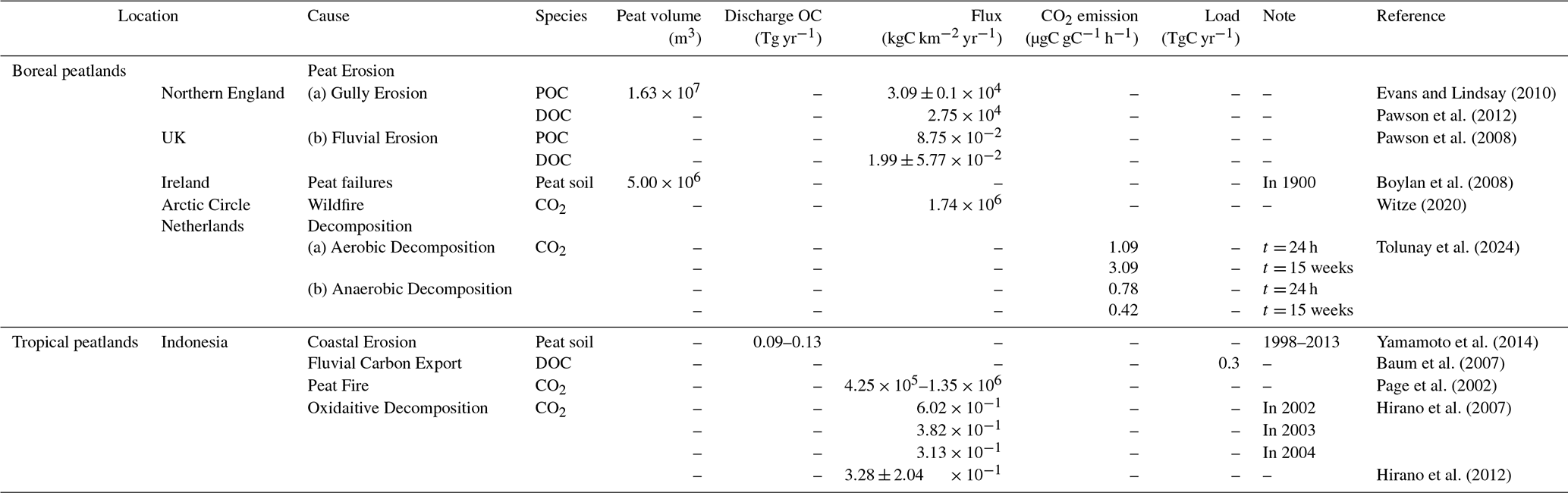
However, these ecosystems are increasingly threatened by deforestation, drainage, and fire, which are transforming tropical peatlands from persistent carbon sinks into net sources of greenhouse gas emissions (Hooijer et al., 2010; Couwenberg et al., 2010). Table B1 summarizes reported values of carbon export from boreal and tropical peatlands, providing a comparative overview across climatic zones. Lateral degradations in boreal peatlands, such as gully erosion and peat failures, are known to cause large-scale peat discharge (Evans and Lindsay, 2010; Boylan et al., 2008). The POC export flux associated with gully erosion has been reported as 3.09 ± 0.1 × 10⁴ gC km−2 yr−1 (Evans and Lindsay, 2010). In contrast, tropical coastal peatlands experience substantial peat loss driven by coastal erosion (Yamamoto et al., 2014). In contrast to fire-related emissions, physical degradation processes such as coastal erosion and peat mass movement events (PMMs) have been underrecognized as a pathway of carbon loss from peatland. Recent research has confirmed that tropical coastal peatlands are undergoing substantial degradation and loss due to coastal geomorphological processes, such as erosion retreat and peat bog burst. Yet, this pathway remains unquantified, especially in contrast to the well-documented fluvial peat erosion processes in boreal and Arctic peatlands (Nabilah et al., 2024). The lack of long-term monitoring of coastal processes and the low number of reported failure events also contribute to this unresolved situation. For example, on Bengkalis Island, the degradation of mangrove vegetation has left peat cliffs exposed to direct tidal and wave forces, leading to toppling failures, rotational slides, and cantilever collapses (Basir et al., 2024). These failures may represent a direct and measurable pathway for the export of particulate organic carbon (POC) to adjacent marine systems; however, the spatial extent and magnitude of this process remain poorly understood.
While lateral erosion and mass movements have been well studied in boreal and Arctic peatlands, distinct mechanisms are observed in those regions (Lantuit et al., 2011; Lantuit and Pollard, 2008; Yunker et al., 1991; Rachold et al., 2002; Lehfeldt and Milbradt, 2000; Sterr, 2008; Nicholls and Cazenave, 2010; Wong et al., 2014; Chambers et al., 2019; Malpica-Piñeros et al., 2024; Chevallier et al., 2023; Dykes and Warburton, 2007; Bowes, 1960; Warburton et al., 2004; Dykes and Jennings, 2011; McCahon et al., 1987; Alexander et al., 1986; Wilford, 1966). For example, erosion along the Bykovsky Peninsula in Siberia is driven by thawing of ice-rich permafrost and storm surges, with buried Holocene peat and ice wedges commonly found in the stratigraphy (Lantuit et al., 2011). Similarly, Arctic coasts in Alaska experience cryogenic processes influenced by permafrost degradation, brackish water, and short ice-free seasons.
In the southern Baltic Sea region, another contrasting model is observed, where Holocene sea-level rise and wave-induced abrasion have eroded glacially derived peat layers overlying lacustrine and glacial till sediments (Furmanczyk and Dudzińska-Nowak, 2009). In the British Isles, raised and blanket bogs – shallow, ombrotrophic peatlands reliant on precipitation – frequently exhibit failure modes such as bog bursts and bog flows (Dykes and Warburton, 2007; Boylan et al., 2008). For example, coastal landslides on Bengkalis Island have closely resembled bog bursts reported in boreal regions (Yamamoto et al., 2019a), and the residual landforms display crack patterns characteristic of progressive failure – a mechanism well established in rock mass collapse (Bjerrum, 1967). However, the landscape of the failure site differs fundamentally, occurring in coastal lowlands rather than upland terrain typical of boreal peatlands. Documented events – such as the peat landslide on Bengkalis Island (Yamamoto et al., 2019a) and the 1966 failure in Malaysia (Wilford, 1966) – suggest that tropical PMMs may share morphological features with boreal failures yet arise under distinctly different hydrological and hydraulic regimes. Despite these differences, the implications for carbon cycling may be broadly comparable.
Global POC export from riverine systems is estimated at 110–230 MtC yr−1 (Galy et al., 2015). Meanwhile, erosion of organic-rich soils–including peat–has increasingly been recognized as a major contributor to the marine carbon budget (Hilton et al., 2015). Particularly in tropical coastal zones, the direct mobilization of peat-derived POC into adjacent seas may represent an underrecognized component of land-to-ocean carbon flux. If ultimately buried in marine sediments, this exported material could function as a long-term carbon sink.
This study focuses on Bengkalis Island as a representative system of tropical coastal peatland degradation. We investigate geomorphic changes associated with coastal erosion and PMMs, with the goal of quantifying the resulting export of POC. By situating these findings within a broader biogeographic and geoclimatic context, this study addresses a critical gap in our understanding of the role of tropical coastal peatlands in global carbon cycling. To support this analysis, we employ a conceptual model (Figs. 1 and 2) that integrates coastal erosion processes and PMMs.
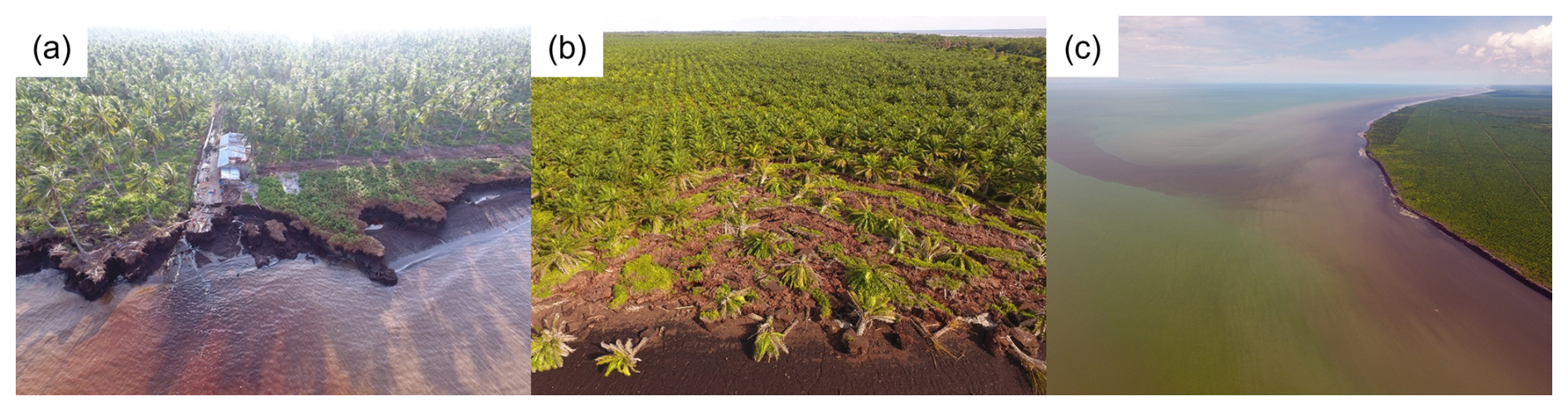
Figure 1Example of lateral degradations in tropical coastal peatland. (a) Coastal erosion (Rangsang Island, Indonesia); (b) Peat mass movement events (Bengkalis Island, Indonesia); (c) Situation where peat is discharged into the ocean due to lateral degradations (Bengkalis Island, Indonesia).
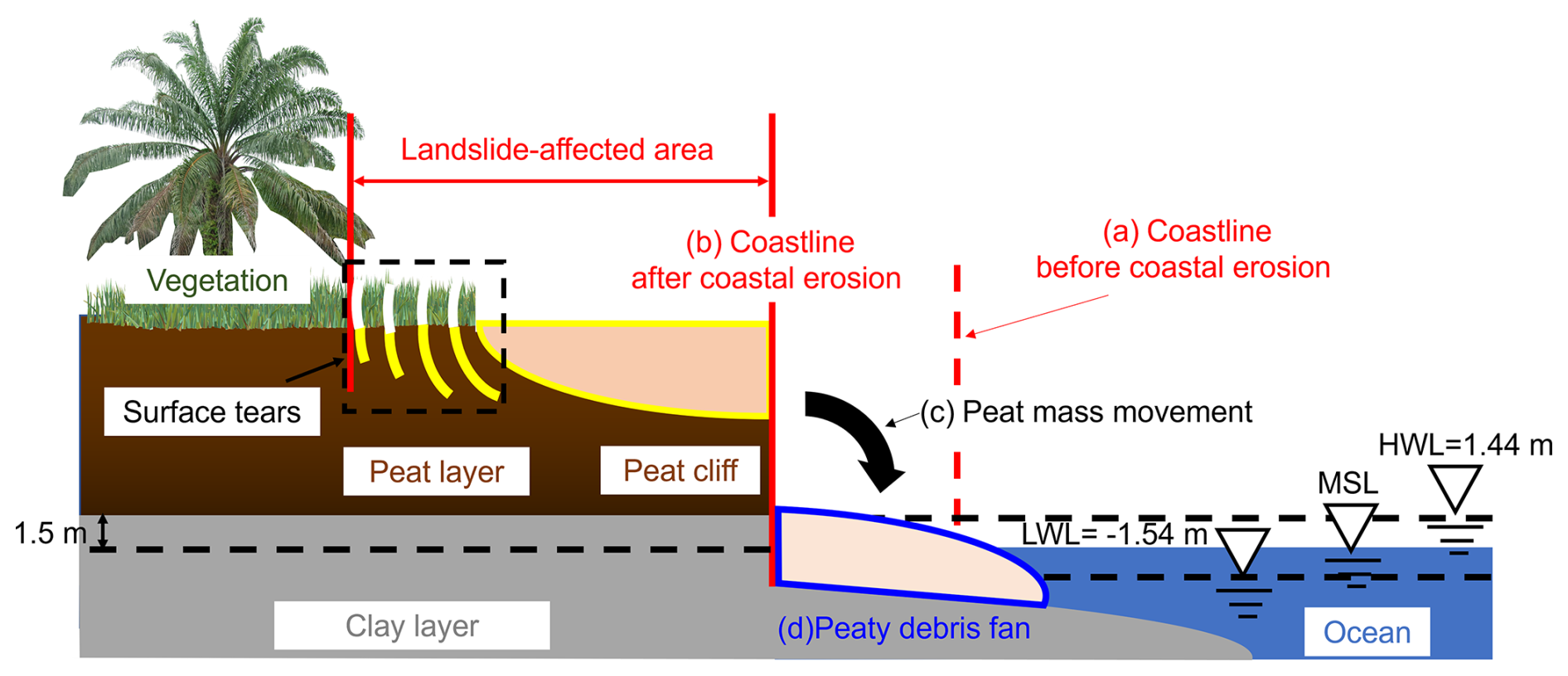
Figure 2Conceptual figure of coastal erosion and PMMs on the peatland coast. Where the High-Water Level (HWL) is 1.44 m, the Mean Sea Level (MSL) is 0 m, and the Low Water Level (LWL) is −1.54 m. (a)–(d) shows the transitional changes in the coastal landform and a cross-section of the coast. (a) coastline before coastal erosion; (b) coastline after coastal erosion; (c) trace of where PMM occurred; and (d) peaty debris fan formed by peat overhanging the coastline due to the occurrence of PMMs. When PMMs occur, cracks through the peat layer, known as surface tears, appear in the hinterland. In this study, the area affected by the landslide was defined as the hinterland from the peaty debris fan to the head of the source of surface tears. Landslide-affected areas have a thinner vegetation cover.
Bengkalis Island in Riau Province, Indonesia, is a tropical coastal peatland island that encompasses the Straits of Malacca and Bengkalis located 1.6° N and 102° E, covering an area of approximately 900 km2 (Fig. 3). Local observations from 2015 to 2018 recorded annual precipitation ranging from 1381 mm to 2402 mm. With peat accumulation dating back 5000 to 6000 years, the island is characterised by its flat topography and is composed primarily of five peat domes, reaching a maximum elevation between 10 and 15 m above sea level (Supardi et al., 1993). Since 1988, land use trends on the island have changed considerably. In 2019, oil palm plantations had expanded to cover 31.12 % of the island's total area, accompanied by the construction of waterways designed to transport oil palm fruit bunches (Umarhadi et al., 2022).
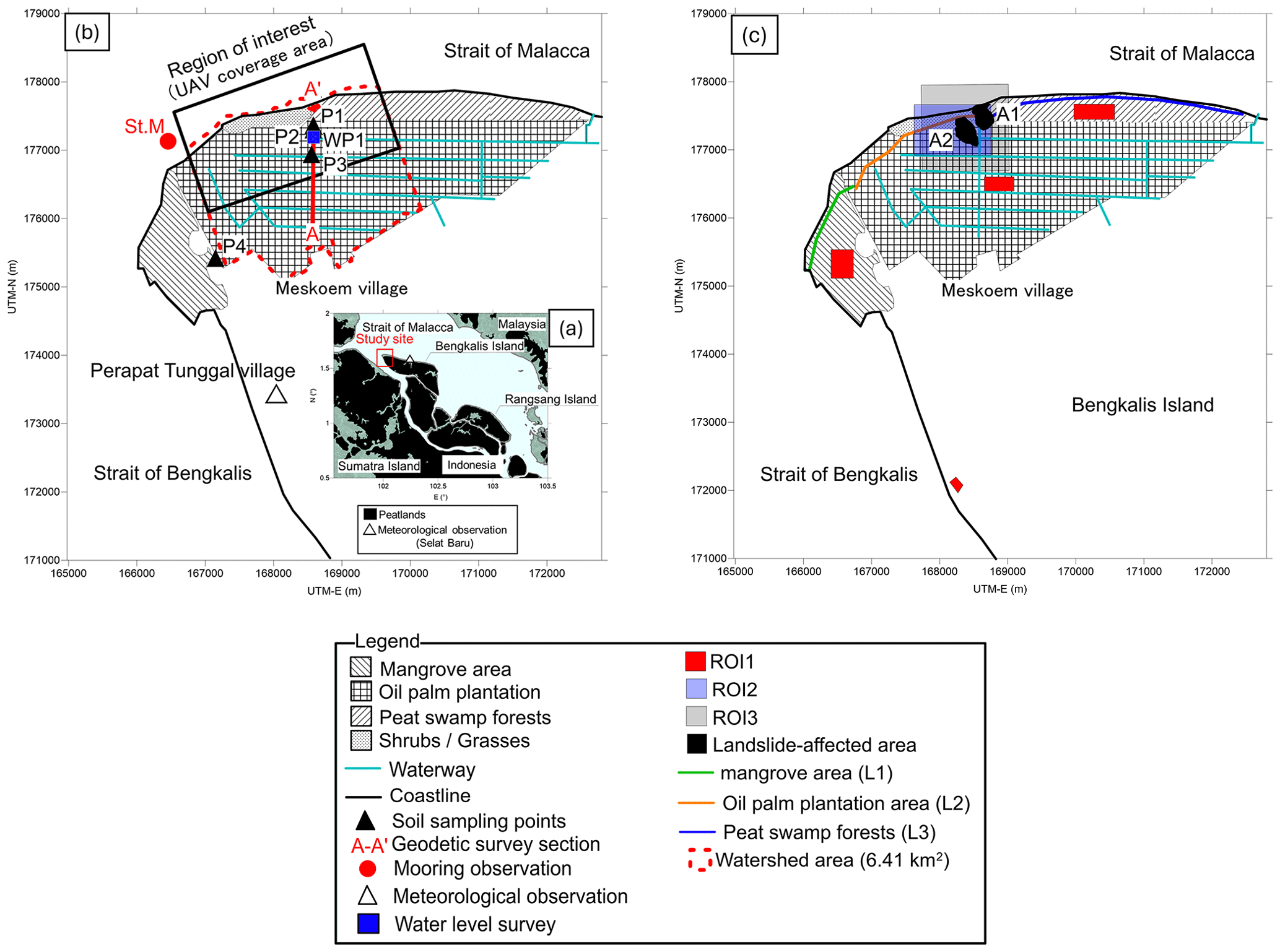
Figure 3Location of the study site (northwest coast of Bengkalis Island). The peat area is delineated referring to Xu et al. (2017). The northern coast of the island is the area eroded by coastal erosion. The classification of land use is based on field observation. (a) provides a regional overview of the study area, (b) identifies the locations of the field survey sites, and (c) shows the sites used for the remote-sensing analysis. ROI1 indicates the area used for the comparison of NDVI between Landsat 8 and Sentinel-2, ROI2 represents the area used to examine the relationship between NDVI and vegetation cover, and ROI3 denotes the area used to identify the timing of occurrence using SAR imagery.
Currently, the northwest area of Bengkalis Island is experiencing considerable coastal erosion. The coastline gradually approached the highest area of the peat dome on northwest Bengkalis Island. Satellite imagery analysis from 22 December 1988 to 18 July 2013, revealed a coastal erosion rate of approximately 34 m yr−1 (Kagawa et al., 2017). Maps created by the US Army Map Service (1955) documented the presence of mangrove belts on all northern coasts. However, these mangrove belts cover only a limited area of the northwest coast, revealing the erasure of inland peatland forests facing the sea and the formation of approximately 6 m tall peat cliffs. Furthermore, the island experienced an average subsidence rate of 2.646 ± 1.839 cm yr−1 between 2018 and 2019, with the northwestern part recording significant subsidence rates of up to 17.416 cm yr−1 due to peat bursts (Umarhadi et al., 2022).
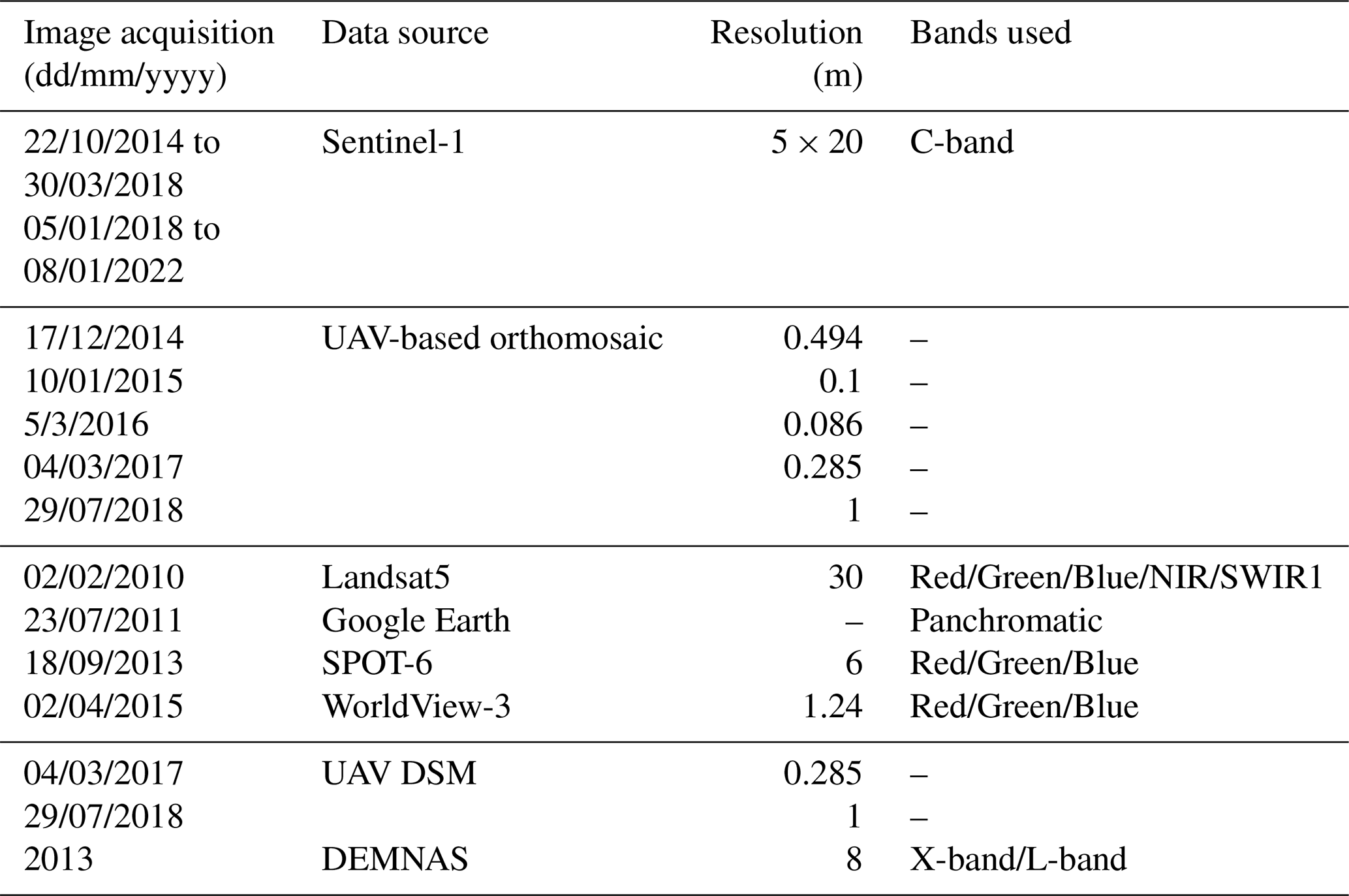
The methodology of this study consists of (Fig. 4): (a) To clarify the actual state of PMMs, we identified the timing of their occurrence, (b) To clarify the actual state of coastal erosion, we estimated the coastline retreat, (c) estimation of barren land area using machine classification satellite images, (d) modification of the digital surface model (DSM) to a digital terrain model (DTM), (e) estimation of the POC from the displacement of peat mass caused by PMMs using field surveys and satellite image analyses, and (f) estimation of the specific annual POC export due to coastal erosion using field survey and satellite image analysis. And the meanings of the abbreviations appearing in this study are given in Table 1 and Fig. 5. In this study, multispectral and panchromatic satellite imagery, aerial photogrammetry, DSM data, cross-sectional land surveys and soil sampling were used to assess coastal and peatland degradation. Table 2 lists the images used in this study. Combining the above steps in Sect. 3.2.1 through 3.2.6 yields the overall workflow depicted in Fig. 4.
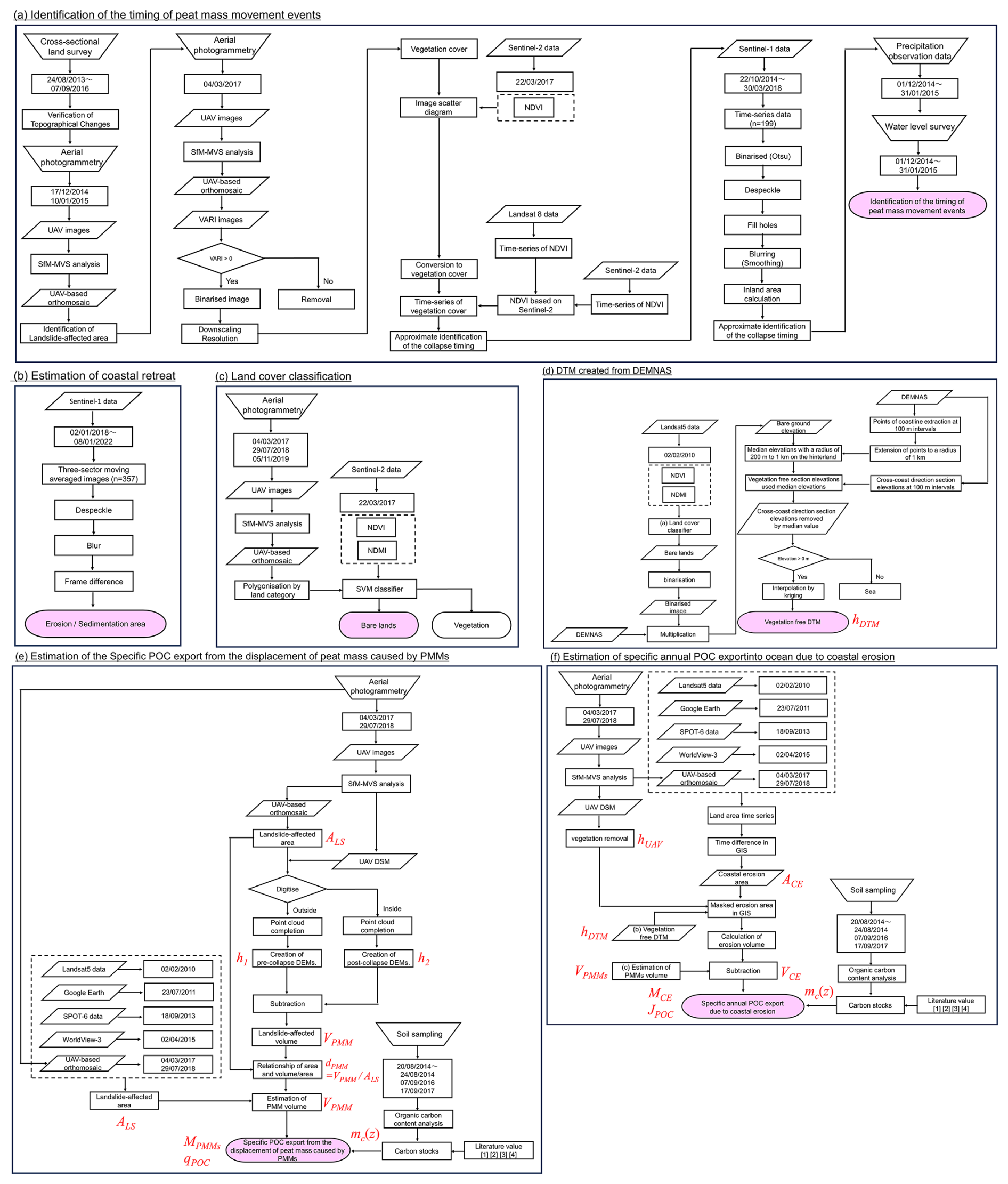
Figure 4Flow chart used in this study for field surveys and satellite image analysis; (a) To clarify the actual state of PMMs, we identified the timing of their occurrence; (b) To clarify the actual state of coastal erosion, we estimated coastline retreat; (c) an estimation of barren land area by machine classification satellite imaging; (d) the modification of a digital surface model (DSM) to a digital terrain model (DTM). Abbreviations used: hDTM – Elevation of DTM; (e) and estimation of POC from displacement of peat mass caused by PMMs. Abbreviations used: ALS – Landslide-affected area, h1 – Elevation before landslide, h2 – Elevation after landslide, VPMM – Peat mass movement volume, dPMM – Depth of affected by landslide, mc(z) – Carbon stocks, MPMMs – Mass of POC due to PMMs, qPOC – specific POC export to ocean due to PMMs; (f) an estimation of the specific annual POC export due to coastal erosion; Literature values [1] [2] [3] [4] sourced from Wahyunto et al. (2003); Dariah et al. (2013); Warren et al. (2012) and Rudiyanto et al. (2018). Abbreviations used: hUAV – Elevation of DSM from UAV photogrammetry, ACE – Coastal erosion area, hDTM – Elevation of DTM, VPMMs – Peat mass movements volume, VCE – Coastal erosion volume, mc(z) – Carbon stocks, MCE – Mass of POC due to coastal erosion, JPOC – Specific annual POC export to ocean due to coastal erosion.
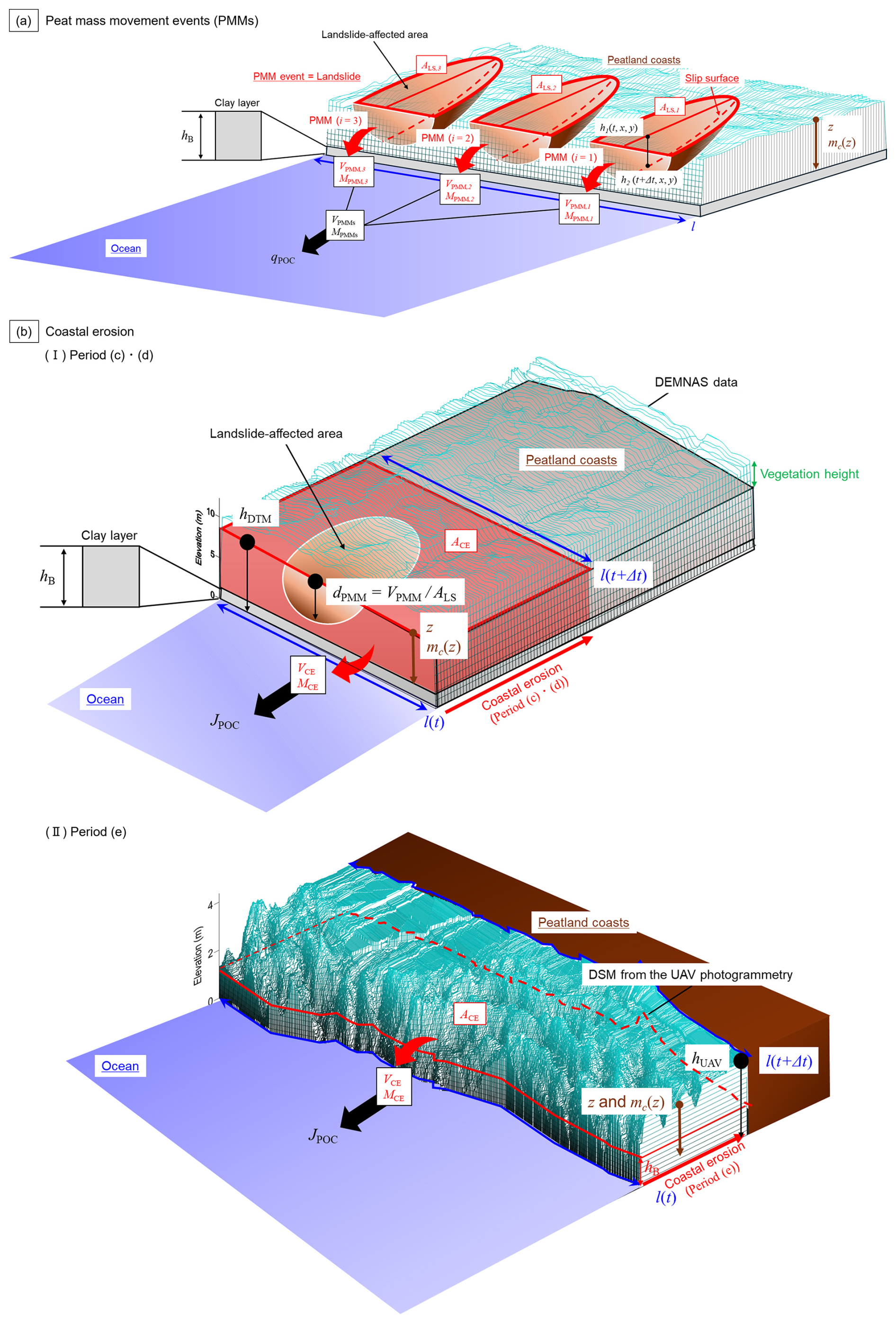
Figure 5Illustrative image of abbreviations. (a) Model of abbreviations associated with peat mass movement events; (b) Model of abbreviations associated with coastal erosion.
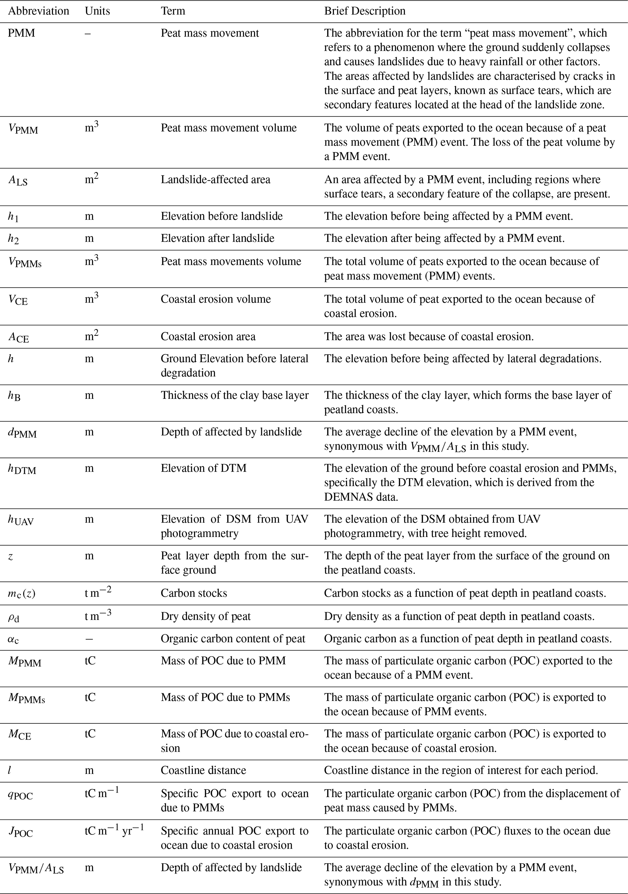
Table 2Remote sensing data used in this study. Satellite imagery data was used in addition to UAV-based orthomosaic and DSM from the aerial photogrammetry results of the field survey.
3.1 Materials
3.1.1 WorldView satellite data and Google Earth image
To identify areas of coastal erosion and PMMs, Google Earth images captured on 23 July 2011 and WorldView-3 multispectral data from 2 April 2015, were used. Launched on 13 August 2014, WorldView-3 operated from a circular sun-synchronous orbit at an altitude of 617 km. WorldView-3 provides eight bands of multispectral data at resolutions of 1.24 (nadir) and 1.38 m (20° off-nadir), and hence a revisit frequency of 4.5 d. Both sensors in the WorldView constellation provide high-resolution Earth observation imagery.
3.1.2 Landsat data
In this study, multispectral Landsat series images, including Landsat 5 Thematic Mapper (TM) and Landsat 8 Operational Land Imager (OLI), were used. Landsat 5 TM images captured on 2 February 2010 were used to delineate coastal erosion and areas affected by landslides. Additionally, Landsat 5 TM imagery was used to extract bare lands. Landsat 5 TM was launched in March 1984 and carries a Multispectral Scanner Subsystem (MSS) and a TM onboard. TM has improved the spectral, radiometric, and spatial resolutions relative to MSS. It aims to provide data continuity to the Landsat Earth observation program, started in the 1970s. These Landsat series data were downloaded from the USGS EarthExplorer (https://earthexplorer.usgs.gov/, last access: 8 February 2026), and the cloud cover in the collected images was 0 %.
3.1.3 Sentinel-1 data
For the identification of the timing of PMM occurrence, Sentinel-1 data acquired from 22 October 2014 to 30 March 2018 were used. The target site is indicated in Fig. 3c (ROI3). In addition, for the estimation of coastal retreat, Sentinel-1 data collected from 5 January 2018 to 8 January 2022 were employed. Sentinel-1 is a constellation of two radar imaging satellites that are part of the European Union's Copernicus Programme. Equipped with C-band synthetic aperture radar (SAR) sensors, Sentinel-1 can capture high-resolution images of the Earth's surface regardless of weather conditions or lighting, making it ideal for continuous monitoring. In its Interferometric Wide Swath mode, it offers a resolution of approximately 5 × 20 m. Its data are used for a variety of applications, including land and ocean monitoring, disaster management, and environmental observation. Data were obtained from USGS EarthExplorer (https://earthexplorer.usgs.gov/).
3.1.4 SPOT-6 data
To elucidate the evolution of PMMs due to coastal erosion, SPOT-6 data captured on 18 September 2013, were used. SPOT-6 provides high-resolution optical images with a resolution of 6 m in multispectral bands. SPOT-6 was launched on 9, September 2012. The satellite is in a nearly circular, sun-synchronous orbit with a period of 98.97 min at an altitude of approximately 694 km. SPOT-6 acquires 12 bit data in five spectral bands: blue, green, red, panchromatic, and near-infrared.
3.1.5 DEMNAS (National Digital Elevation Model in Indonesia)
The National Digital Elevation Model in Indonesia (DEMNAS) is a digital surface model (DSM) that was used to create a vegetation-free DTM for the coastal zone in this study. DEMNAS is the result of interpolation from multiple data sources such as IFSAR, TERRASAR-X and ALOS PALSAR at 5, 5, and 11.25 m resolutions, respectively, with the addition of stereo plotted mass point data in the calculation (EGM2008 vertical datum).
3.1.6 Aerial photogrammetry
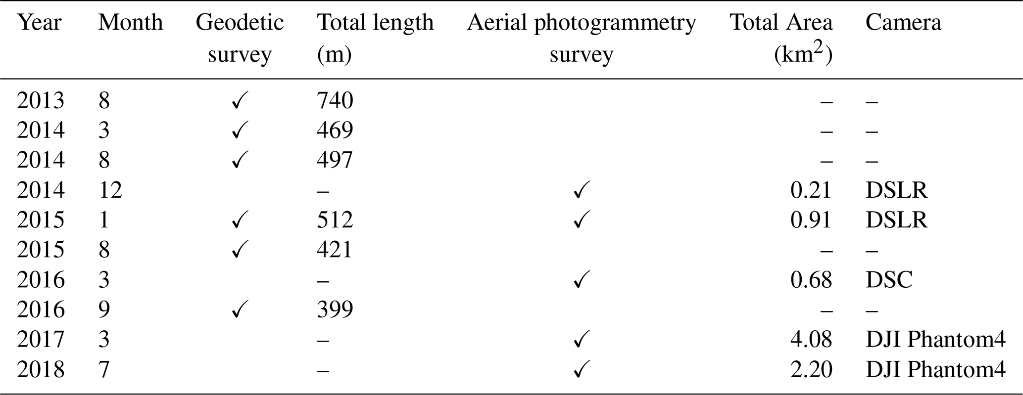
To investigate coastal erosion and PMMs, an unmanned aerial vehicle (UAV) was used for aerial photogrammetry. Figure 3 shows the areas of interest. Table 3 lists the survey schedules, and the equipment used in this study. For photogrammetry, ground control points (GCPs) were established and geolocated using static GNSS measurements (5700/5800, Trimble, USA) or RTK-GNSS (GRX2, Sokkia, Japan). Commercially available software (Photoscan Professional, Agisoft, Russia) was used to process the resulting images for SfM-MVS analysis to create a DSM.
Table 3Geodetic and aerial photogrammetry survey schedule and equipment.
3.1.7 Cross-sectional land survey
To examine changes in the cross-sectional profile of the land, particularly in the plantation in Meskom Village, a survey was carried out along a north–south transect (Section A-A′). Figure 3 displays the transect and Table 3 lists the survey schedules. A Sokkia GRX2 RTK-GNSS system based on reference points located in the Bengkalis state polytechnic was used to perform the measurements.
3.1.8 Sampling and analysis of peat soils
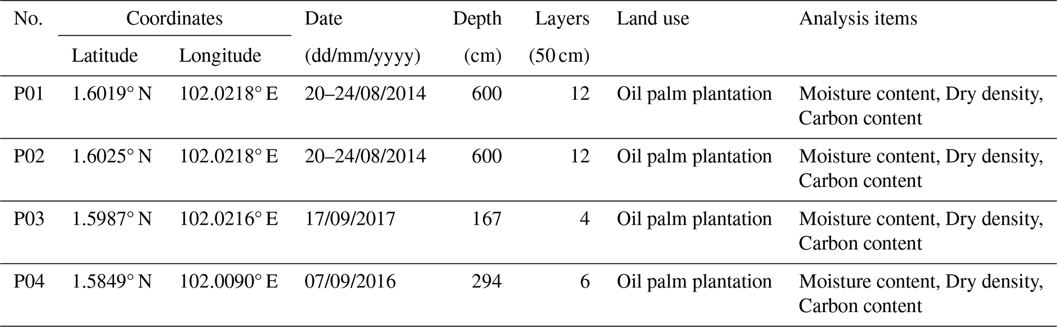
Soil sampling was performed to determine the organic carbon content of the peat soil. Figure 3 shows the sampling points and Table 4 lists the sampling and analysis information. A Dutch-style peat sampler (DIK-105A, Daiki Rika Kogyo Co., Ltd., Saitama, Japan) was used to extract samples up to 6 m below the clay layer. Quantitative sampling was performed to measure the density at the time of collection. The samples were dried at 105 °C and the organic carbon and nitrogen content was analysed using a CHN analyser (JM-10 analyser, J-Science Lab., Kyoto, Japan).
3.1.9 Mooring observations
From 4 November 2019 to 13 January 2020, a pressure-type memory wave gauge (INFINITY-CTW) was moored approximately 500 m offshore from a coast undergoing significant erosion to measure wave heights from the temporal variation in pressure (Fig. 3 (St. M)). Based on these measurements, significant wave heights were calculated for every two-hour interval.
3.1.10 Meteorological observations
To elucidate the temporal characteristics of PMMs occurrences and the features of coastal erosion, meteorological observation instruments were installed at Selat Baru and Perapat Tunggal on Bengkalis Island (Fig. 3), and measurements were conducted. The instruments used were the SESAME II-05d (Midori Engineering Institute). This study utilized data collected from 2014 to 2021.
3.1.11 Water level survey
To investigate changes in water levels within channels in areas where peat collapse occurs frequently, a water level gauge was installed at the location shown in Fig. 3 (WP1). A monitoring well was constructed at the measurement site using a polyvinyl chloride (PVC) pipe, and the channel water level was recorded using a HOBO U-20 water level logger. This study utilized data collected from 1 December 2014 to 31 January 2015.
3.2 Methods
3.2.1 Identification of the timing of PMM occurrence
Time-series NDVI (Normalized Difference Vegetation Index) data were analysed using the Sentinel Hub EO Browser, with average NDVI values calculated within predefined polygons across a specified temporal range to evaluate vegetation dynamics (see Appendix B for details). The relationship between NDVI and vegetation cover was also examined, demonstrating a strong correlation between NDVI values obtained from Sentinel-2 and Landsat 8 imagery (Appendix C). These analyses provide a robust framework for detecting vegetation changes and estimating the timing of peat mass movements (PMMs). In particular, the occurrence of PMMs is often preceded by the formation of surface tears–cracks that appear on the ground surface–leading to a localized decline in vegetation cover. This characteristic reduction in NDVI serves as a key indicator of the onset of PMMs.
Changes in the land area within the landslide-affected areas were analysed using Sentinel-1 SAR images acquired between 22 October 2014 and 30 March 2018. The time-series data were downloaded as an animated GIF from the EO Browser, in the region of interest is shown in Fig. 3. The image analysis procedure involved applying a moving average over three consecutive acquisition intervals and smoothing the coastline using a blurring technique. Subsequently, noise within the region of interest was removed. After blurring, the images were binarized to isolate the land areas, thereby revealing changes in the extracted region. The expansion of this area a characteristic feature of peaty debris fans occurs following peat mass movement events.
3.2.2 Estimation of coastal retreat using SAR image
Using 359 Sentinel-1 SAR images acquired from 5 January 2018 to 8 January 2022, the average cumulative coastline retreat was calculated for each land cover type namely, the mangrove belt, oil palm plantation, and peat swamp forest. The specific coastlines corresponding to these land cover types are shown in Fig. 3, and the analytical workflow is illustrated in Fig. 4.
The analysis procedure was as follows. First, a moving average was applied over three consecutive acquisition intervals (including the day before and after each image) to smooth the data. Next, the coastline and land areas were separated by binarization. Noise reduction was then performed, and the difference between consecutive images was computed to extract the regions undergoing coastline changes. The area of these regions was calculated, and by dividing the computed area by the corresponding coastline length for each land cover type, the average coastline retreat was determined.
For 2018 and 2021, local observations (Fig. 3) of precipitation and wind speed were summarized as annual precipitation and annual maximum wind speed. Furthermore, the relationship between significant wave height and maximum wind speed was examined for the period from 4 November 2019 to 13 January 2020 using data from mooring observations. In analysing maximum wind speed, data recorded at Selat Baru were used; since the moored observation points differed, a moving average covering two hours before and after each observation was applied to better represent the relationship between significant wave height and maximum wind speed.
Additionally, annual wind roses were generated using 10-minute interval observations of maximum wind speed and direction recorded at Selat Baru and Perapat Tunggal in 2018 and 2021. These combined meteorological and remote sensing analyses allowed for a comprehensive discussion of coastal erosion characteristics across different land cover types.
3.2.3 Estimation of the volume of exported land slide-induced peat to the ocean
Aerial photogrammetry-derived DSMs were used to establish the relationship between the area and the loss of the peat volume by PMMs. This relationship was then used to estimate the losses in peat volume in areas affected by landslides identified in multispectral satellite imagery. Elevations before and after collapse were obtained by manually digitising the edges and inside the landslide-affected area within the GIS software (QGIS ver. 3.20) using orthomosaics and DSMs resulting from aerial photogrammetry carried out on 4 March 2017 and 29 July 2018, respectively, and within Estimation of the volume of export of land slide-induced peat to the ocean (Fig. G1g, G1h). The landslide-affected areas were judged by the characteristics of the ground, such as surface tension cracks or the presence of peat blocks. Tension cracks and irregular peat blocks are some of the characteristic features of peat mass movements (Warburton et al., 2004). Two digital elevation models (DEMs) were generated using aerial photogrammetry results. The first DEM was the initial land surface, which was recreated by interpolation using elevations of the points extracted from the edges of the areas affected by landslides within the DSM (Fig. G1g). The second DEM was the post-collapse DEM, which were generated by sampling elevation data in areas affected by landslides in the vegetation removed DSM (Fig. G1f, G1h and G1i). The volume of peat exported to the sea due to collapse was deduced by calculating the difference between the first DEM and the second DEM. The method to calculate the volume of peat exported by a PMM event is expressed in Eq. (1),
where VPMM,i represents the volume of peat exported to the ocean by a PMM event i (m3), ALS,i represents the area i affected by the landslide (m2), h1 represents the elevation before the landslide (m), h2 represents the elevation after the landslide (m), x and y represent the distance (m), t represents the change in time.
3.2.4 Estimation of the volume of peat exported by the PMMs using optical satellite images and UAV-based orthomosaic
Landslide-affected areas were extracted from optical satellite images and orthomosaic based on UAVs (Fig. G1a, G1b, G1c, G1d and G1e). When landslide-affected areas were extracted from multispectral satellite imagery, areas with sparse vegetation were spotted using the true colour image and the false colour image (Fig. G1a, G1b, G1c, and G1d). The volumes of peat exported by landslide were estimated in these areas based on a previously determined area–volume/area relationship. Landslide-affected area: ALS,i calculation was performed in the GIS software. The total amount exported to the ocean by PMMs: the VPMMs are shown in Eqs. (2) and (3).
where ALS,i represents the area i affected by the landslide (m2). f represents a function to estimate the volume of the Landslide-affected area. This study considered traced errors in landslide-affected areas, which were calculated by manual tracing in GIS software (Fig. H1). We evaluated the errors caused by differences in resolution using satellite images from Landsat 8 and Sentinel-2 acquired at the same time (n= 7). To achieve this, we conducted 20 tracings per time for comparison (Fig. I1).
3.2.5 Calculation of coastal erosion volume
Accurate estimation of coastal erosion volume required detailed land cover classification and the removal of vegetation from elevation data. Appendix D outlines the land cover classification methodology based on machine learning, employing NDVI (Normalized Difference Vegetation Index) and NDMI (Normalized Difference Moisture Index) derived from Sentinel-2 imagery to differentiate between bare ground and vegetated areas. Appendix E describes the procedure for vegetation removal from DEMNAS elevation data in order to generate a Digital Terrain Model (DTM), thereby eliminating the influence of tree canopy height on surface elevation. These preprocessing steps provided a refined baseline essential for improving the accuracy of coastal erosion volume estimation.
To elucidate the area and volumetric magnitude of peatland loss due to coastal erosion, we drew coastlines using GIS software (QGIS 3.10) based on satellite images, orthomosaic results from aerial photogrammetry, and analysed their temporal changes. The defining equation to calculate coastal erosion is shown in Eq. (4).
where VCE represents the volume of peat exported by coastal erosion in each period (m3), h represents the elevation of the ground before coastal erosion and PMMs (m), hB represents the thickness of the clay base layer (m), ACE represents the area eroded by coastal erosion (m2) and dPMM represents the average elevation drop by a PMM event (m). dPMM is described by the following Eq. (5).
where VPMM represents the volume of peat exported to the ocean by a PMM event (m3), and ALS represents the landslide-affected area (m2).
Multispectral satellite imagery from Table 2 and orthomosaic results from aerial photogrammetry were used to plot the coastlines. For period (c), from 18 September 2013 to 2 April 2015, and (d) from 2 April 2015 to 4 March 2017, the ground elevations before the erosion were determined using the DTM derived from the DEMNAS data. During period (e), spanning from 4 March 2017 to 29 July 2018, ground elevations were obtained from a DSM generated using aerial photogrammetry results obtained from the UAV. The DSM of the UAV photogrammetry was adjusted to remove the height of the tree prior to use. The process of excluding tree heights from the DSM was carried out by checking trees on a UAV-based orthomosaic. Furthermore, the DSM of the UAV was corrected using the root mean square error (RMSE) values of the DTM generated from the RTK-GNSS and DEMNAS data. DTM using DEMNAS data does not consider landslide-affected areas, so landslide volumes are subtracted, but DSM from aerial photogrammetry results reflect spilt volumes due to landslides, so landslide volumes were used as they are, without subtraction. The volume of peat exported by coastal erosion, estimated using DTM, and the volume of peat exported by coastal erosion, estimated using DSM from UAV photogrammetry, are shown in the Eq. (6).
where VCE represents the volume of peat exported by coastal erosion in each period (m3), hDTM represents the elevation of the ground before coastal erosion and PMMs, that is, the elevation of DTM (m), hB represents the thickness of the clay base layer (m), ACE represents the area eroded by coastal erosion (m2), and dPMM represents the average decrease in elevation due to a PMM event (m). hUAV stands for the elevation of the vegetation-free DSM based on the UAV photogrammetry (m). This study considered traced errors in coastal erosion areas, which were calculated by manual tracing in GIS software (Fig. H1).
3.2.6 Estimation of POC mass by PMM event and estimation of specific annual POC export due to coastal erosions
The mass of the POC by the displacement of peat mass caused by PMMs and the specific annual POC export due to coastal erosions were calculated by the spatial distributions of the loss of the peat volume and depth-dependent carbon stocks of the peat. The carbon stocks of peat mc(z) (t m−2) until the depth z (m) of the peat from the surface of the ground was calculated using the following Eq. (7),
where ρd represents the dry density (t m−3) and αc represents the organic carbon content (–). They were combined from the results of field surveys with the value of the literature obtained from Wahyunto et al. (2003); Dariah et al. (2013); Warren et al. (2012) and Rudiyanto et al. (2018).
The mass of POC caused by a PMM event was calculated using Eq. (8),
where MPMM (tC) represents the mass of POC, the variable dPMM represents the average decrease of elevation by a PMM event (m), and ALS represents landslide-affected area (m2). The amount of specific POC export by the PMMs (tC) in each period was calculated using the Eq. (9),
where MPMMs (tC) represent the mass of specific POC export by the PMMs in each period. The mass of POC which is exported to the ocean caused by coastal erosion in each period was calculated using the Eq. (10). Equation (10) is divided into two cases for elevation h (m) before coastal erosion and a PMM event: the case using DTM and the case using UAV aerial photogrammetry results.
where MCE represents the mass of POC caused by coastal erosion (tC), hDTM represents the elevation of the ground before coastal erosion and PMMs, i.e. the elevation of the DTM (m), hB represents the thickness of the clay base layer (m), ACE represents the eroded area by coastal erosion (m2) and dPMM represents the average decline of the elevation by a PMM event (m), and hUAV represents the elevation of the DSM from the UAV photogrammetry was removed tree height (m). The POC from the displacement of peat mass caused by PMMs and from fluxes due to coastal erosion were calculated using Eqs. (11) and (12), where qPOC (tC m−1) represents the POC from the displacement of the peat mass caused by PMMs. JPOC (tC m−1 yr−1) represents the specific annual POC export due to coastal erosion, l (m) represents the coastline distance, Δt (yr) represents the years of interval for coastal erosion. The POC from the displacement of peat mass caused by PMMs was not measured by fluxes, as PMMs are a sudden disaster. Instead, it was calculated based on the areas that had already collapsed by each date. In general, peat mass movements in boreal peatlands only uses the unit without time such as m3 or tons to evaluate the magnitudes of these events (Dykes and Warburton, 2007).
The calculated POC shows the standard deviation (SD) of five patterns, including the values from the literature.
4.1 Characteristics of landslide-affected area
An analysis of the correlation between the area and volume/area of PMMs from 2017 to 2018 in the coastal area of the oil palm plantation is presented in Fig. 6 and Eqs. (13), (14), where VPMM represents the loss of peat volume by PMMs (m3), and ALS represents the landslide-affected area (m2).
A linear relationship was observed between the landslide area and volume of the peatlands. If the is assumed to be the depth of the landslide-affected area, the higher the ALS, the deeper the depth of the collapse. When collapse also occurs, it will be as deep as 1 m. The smallest collapse had an area of 0.11 × 10⁴ m2 and a volume of 491 m3. The largest collapse had an area of 3.70 × 10⁴ m2 and a volume of 85 173 m3. On average, the landslide-affected areas measured 1.51 × 10⁴ m2 in area and 22 546 m3 in volume. The relationship between the volume exported to the ocean by peat mass movements (VPMM) and landslide-affected area (ALS) on Bengkalis Island indicates that the average reduction in ground level (), which ranged from 0.94–1.93 m (mean value = 1.33 m), increased with the area of landslide-affected area (ALS). The ground-level drop was found to be around 0.91 m in small collapses. The depths of peatland degradation varied, but typically in boreal peatlands, blank peat degradation occurred at a depth of 0.6–3 m (Warburton et al., 2004). Koyama et al. (2018) performed geotechnical investigation results in the northwest of Bengkalis Island and revealed a tendency for sedimentary peat to be less than approximately 2 m below groundwater level and the penetration strength to decline. Furthermore, the average difference between the pre-collapse ground elevation and the bottom surface of the peatland cracks was 2.01 m, which indicates a possible correlation between the peatland degradation slide surface and sedimentary peat location.
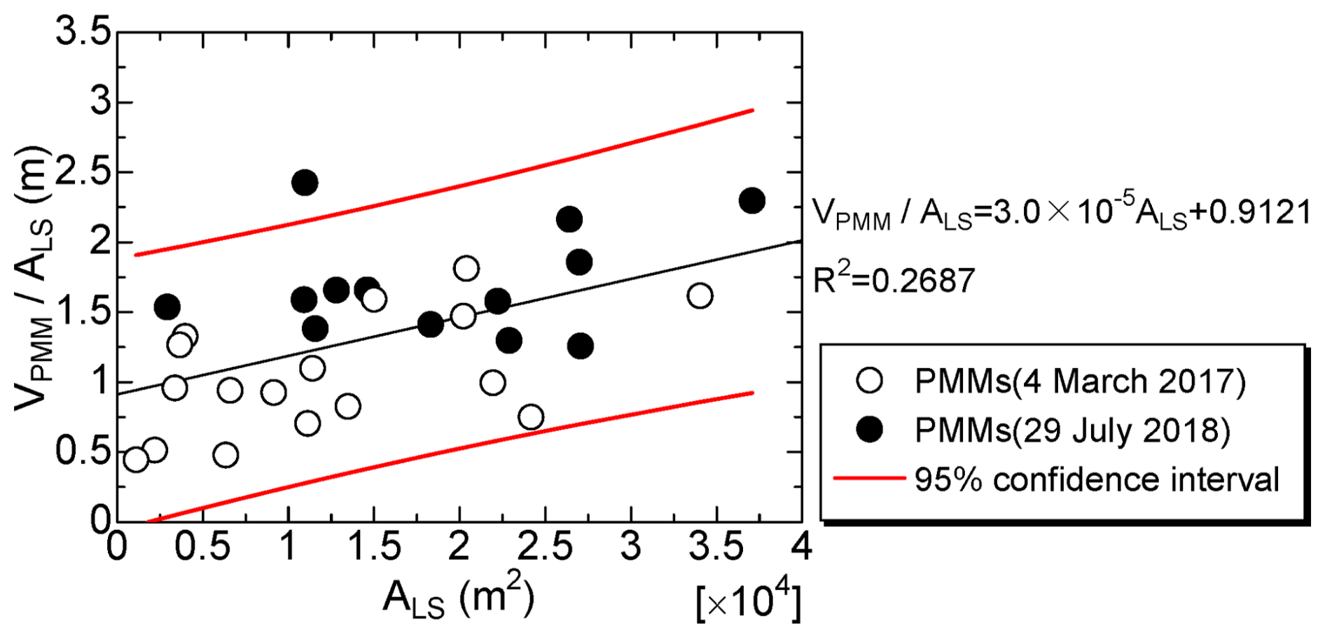
Figure 6Area-Volume/Area relationship of a peat mass movement event. Where, ALS is landslide-affected area, VPMM is the loss of the peat volume due to a PMM event. There is a linear relationship between ALS and ; If is assumed to be the depth of landslide-affected area, the greater the ALS, the deeper the depth of the collapse. It was found that the ground level drop was around 0.91 m in small collapses.
4.2 Identification of the timing of peat mass movement events
Figure 7 shows the temporal changes in elevation along survey section A–A′. Variations in elevation indicate the occurrence of surface tears. In the section corresponding to UTM-N from 177 300 to 177 400 m, the elevation decreased by an average of 2.01 m between 24 August 2013 and 11 March 2014. UAV-based aerial photogrammetry conducted on 17 December 2014 revealed that a peat collapse had occurred (Fig. 3c (A1)).
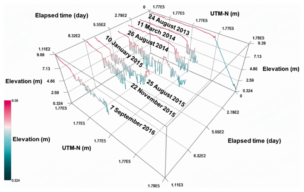
Figure 7The change in temporal elevation in Section A-A'. The elevation decreased due to PMM since 24 August 2013.
Figure 8 displays an image obtained by SPOT-6 satellite imagery, UAV-based orthomosaic images and calculating the Visible Atmospherically Resistant Index (VARI) from UAV-based orthomosaic image in which only the exposed peat substrate is delineated. The extent of this PMM was estimated at 8.95 × 10⁴ m2 in area, with a volume of 321 940 m3, an aperture length of 296 m, and a length of 379 m. The landslide-affected area spans peat swamp forests, oil palm plantations, and shrublands. Furthermore, since 18 September 2013, the coastline has extended seaward, forming a fan-shaped deposit of peaty debris.
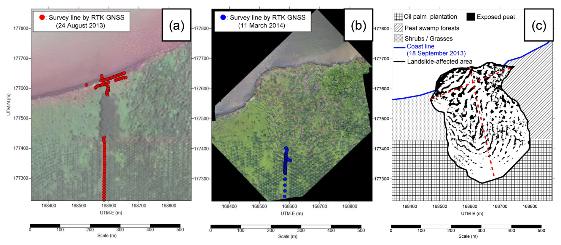
Figure 8(a) SPOT-6 image (18 September 2013) and (b) UAV-based orthomosaic image (17 December 2014), and (c) anatomy of the landslide-affected area. The scale of the landslide-affected area is as follows: the affected area is 8.95 × 10⁴ m2, the volume is 321 940 m3, the length is 379 m, and the aperture length is 296 m. The collapse extended over or into peat swamp forests, oil palm plantations, and shrub areas.
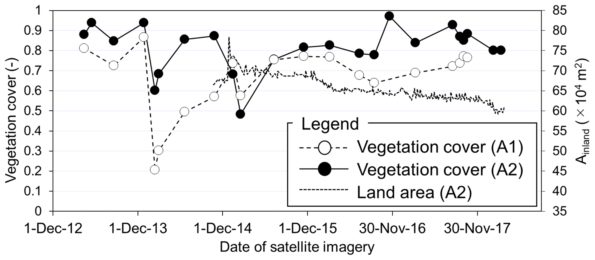
Figure 9Time series of estimated vegetation covers in landslide-affected areas. Vegetation covers rapidly decreased from 27 December 2013 to 13 February 2014, dropping from 0.87 to 0.21 (Fig. 3c (A1)). Similarly, vegetation covers rapidly decreased from 27 October 2014 to 16 February 2015, declining from 0.87 to 0.48 (Fig. 3c (A2)). The land experienced a sudden extension, increasing by approximately 18.4 × 10⁴ m2 between 22 and 28 December 2014 (Fig. 3c (A2)).
Next, the timing of the PMM was determined. In this analysis, the characteristic discontinuity in surface vegetation resulting from the collapse was used to pinpoint its timing. Figure 9 presents the time series of vegetation cover for the peat collapse area identified in Fig. 3c (A1). The vegetation cover dropped sharply from 0.87 on 27 December 2013 to 0.21 on 13 February 2014, indicating that the collapse occurred between these dates.
Moreover, along survey section A–A′ in the UTM-N range from 177 000 to 177 300 m, the elevation decreased by an average of 2.07 m between 26 August 2014 and 10 January 2015 (Fig. 7). UAV-based aerial photogrammetry on 10 January 2015 confirmed that this decrease in elevation was due to a peat (Fig. 3c (A2)). Areas exhibiting fluctuating elevations indicate the presence of peat rafts–blocks of peat displaced by the collapse (Warburton et al., 2004). Figure 10 shows an image obtained by SPOT-6 satellite imagery, UAV orthomosaic images and calculating the VARI from UAV orthomosaic images, with only the exposed peat substrate delineated. In this case, the PMM was estimated to cover an area of 14.9 × 10⁴ m2 with a volume of 0.068 km3, an aperture length of 303 m, and a length of 554 m. The PMM also resulted in the formation of a large peaty debris fan, which had an area of 13.7 × 10⁴ m2, an aperture length of 583 m, and a length of 268 m; the formation of such an extensive fan underscores the large scale of the collapse.
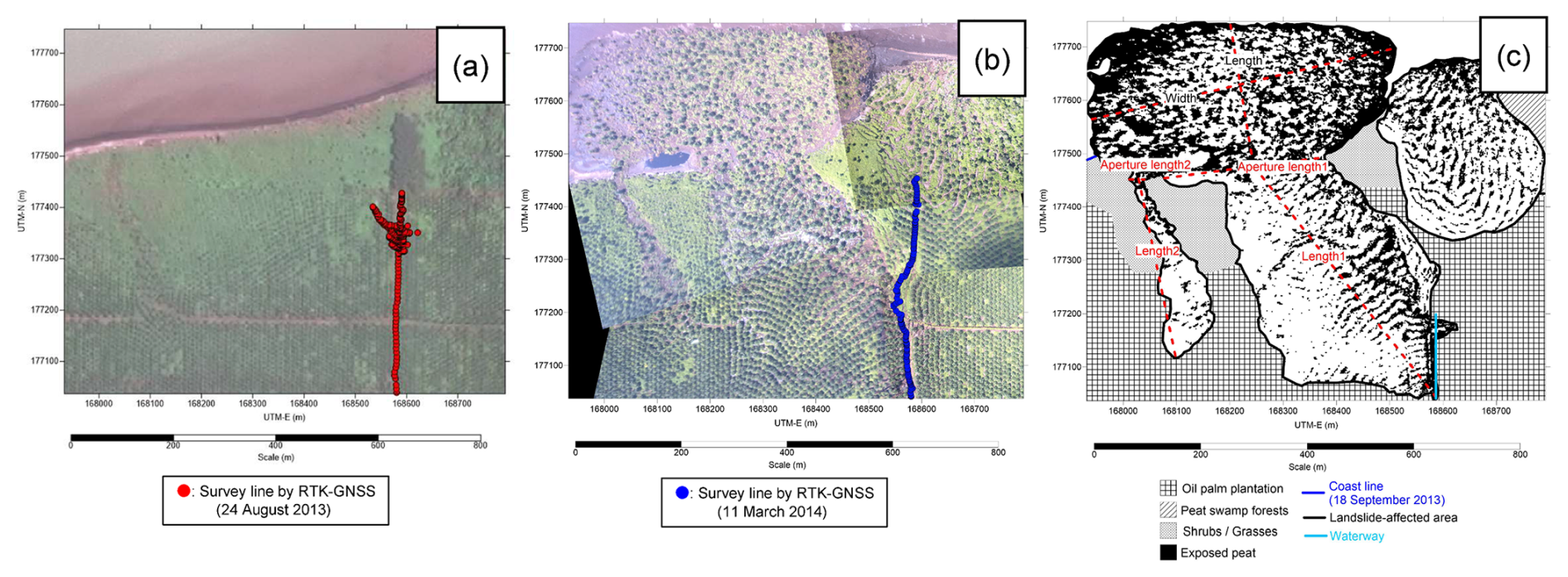
Figure 10(a) SPOT-6 image (18 September 2013), (b) UAV-based orthomosaic image (10 January 2015), and (c) anatomy of the landslide-affected area. The scale of the landslide-affected area is as follows: the area is 14.9 × 10⁴ m2, the volume is 0.068 km3, Length 1 is 554 m with an aperture length of 303 m, and Length 2 is 341 m with an aperture length of 28 m. The scale of the peaty debris fan is as follows: the area is 13.7 × 10⁴ m2, the length is 268 m, and the width is 583 m.
The time series of vegetation cover at the landslide-affected area (Fig. 9) shows that between 27 October 2014 and 16 February 2015 the vegetation cover decreased rapidly from 0.82 to 0.48, suggesting that the PMM occurred during this period. Furthermore, Sentinel-1 satellite imagery indicates that approximately 18.4 ha of land area expanded abruptly between 22 December 2014 and 28 December 2014 (Fig. 9), clearly indicating that a large-scale collapse occurred during this interval.
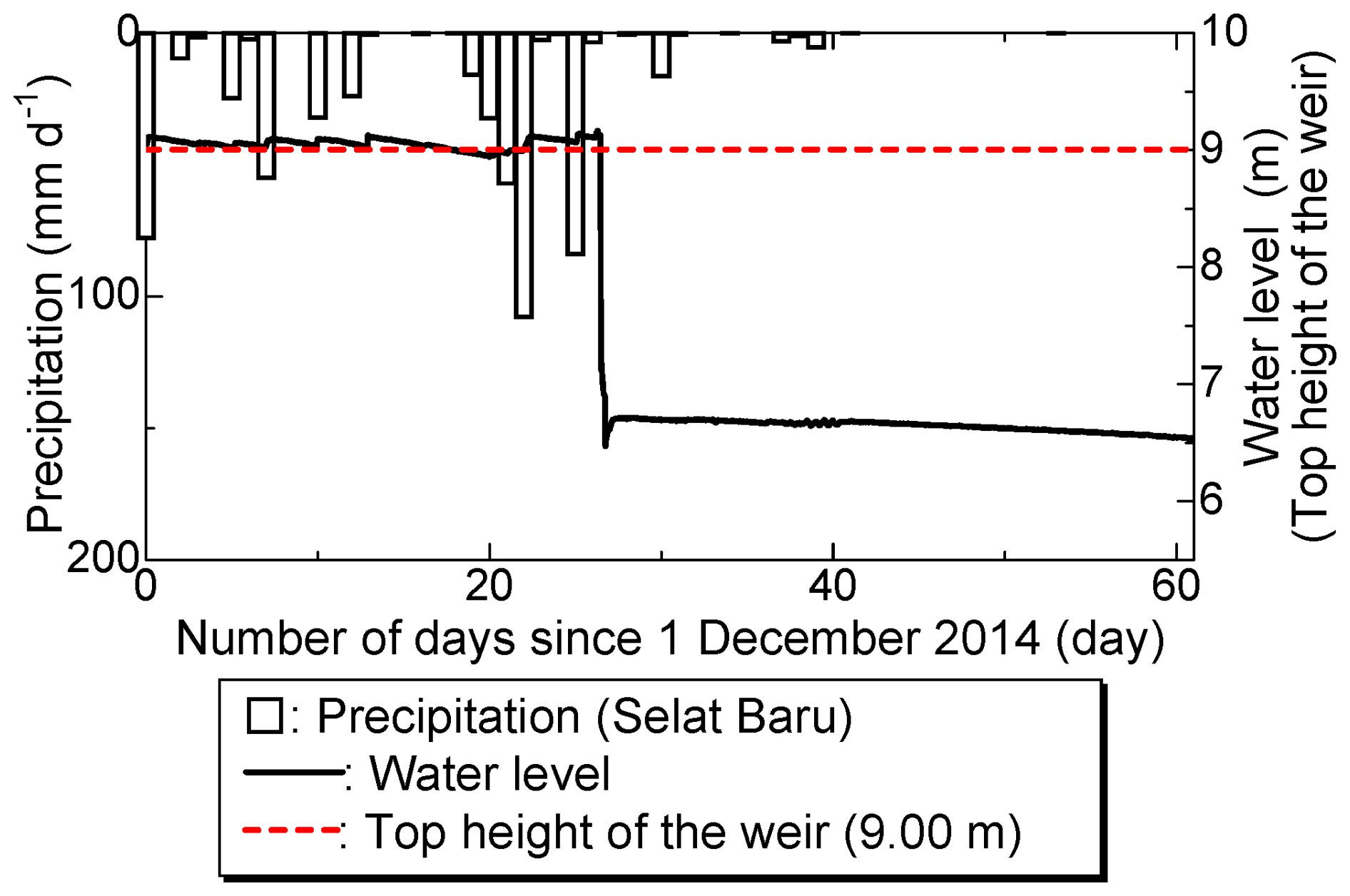
Figure 11Water level of the water way at WP1 and precipitation at Selat Baru station during the peat mass movement event on 27 December 2014. The major precipitation before the event were 107.9 mm d−1 (23 December) and 84.1 mm d−1 (26 December). Subsequently, the water level of the water way dropped suddenly on 27 December 2014. The top height of the weir was 9.00 m, but the water level was recorded at 9.124 m at 11:10 UTC+7 on 27 December 2014, followed by a sudden drop to 7.896 m just 10 min later.
Figure 11 presents the water level data alongside precipitation data from Selat Baru at the landslide-affected area. During the observation period, the maximum precipitation recorded was 107.9 mm d−1 on 23 December and 84.1 mm d−1 on 26 December. Following this record precipitation, the water level in the waterway suddenly dropped on 27 December 2014. Although the crest level of the waterway is 9.00 m, the water level was recorded at 9.124 m at 11:10 UTC+7 on 27 December 2014 and then fell sharply to 7.896 m just ten minutes later (Fig. 11). This abrupt decrease suggests that a breach of the weir occurred between 11:10 and 11:20 UTC+7 on 27 December 2014, triggering the PMM. It was also confirmed that the on-site water level logger had shifted by approximately 30 m. The changes in coastal topography indicate that, because of the PMM, peat was exported into the marine environment. At the study site, continuous precipitation exceeding 20 mm h−1 was recorded from 21 December to 26 December, suggesting that the precipitation after 21 December may have triggered the collapse on 27 December.
Boylan et al. (2008) investigated the relationship between the runout distance and failure volume of 44 recorded peat landslides in northern parts of the United Kingdom (particularly the North Pennines) and throughout Ireland (particularly Connacht and Munster). According to this data, the runout distance generally increases with failure volume, although there is considerable variability. Larger failure volumes and consequently longer runout distances tend to occur in raised bogs, which contain deeper and more extensive peat deposits. The long runout of peat landslides can be transported over long distances when they enter rivers and streams and mix with floodwaters. The runout distance can reach up to approximately 7000 m, and the failure volume can reach up to approximately 10 000 000 m3. Specifically, the PMM in Fig. 8 is smaller in scale than the peat landslides in boreal peatlands. However, compared to the boreal peatland landslides in Fig. 10, it has a shorter runout distance but a volume that is 6.8 times larger.
4.3 Estimation of coastal retreat
Based on the long-term changes observed in SAR imagery, along with local meteorological and mooring observations, the actual state of coastal erosion along the northern coast of Bengkalis Island was elucidated using land cover information and meteorological conditions. Figure 12 shows the cumulative retreat of the coastline by land cover type from 2018 to 2021, as derived from Sentinel-1 data, alongside concurrent meteorological observations. Although coastal erosion has progressed in all land types including mangrove area, oil palm plantations, and peat swamp forests the erosion rate in oil palm plantations is more than twice that observed in mangrove area and peat swamp forests. Moreover, between 2018 and 2021, coastal erosion in oil palm plantations proceeded at an average rate of 3.5 m per 30 d, exceeding the typical average during Indonesia's rainy season, with the highest rate recorded at 24.8 m per 30 d in January 2020. These results suggest that elevated wave heights induced by seasonal winds may accelerate the erosion process.
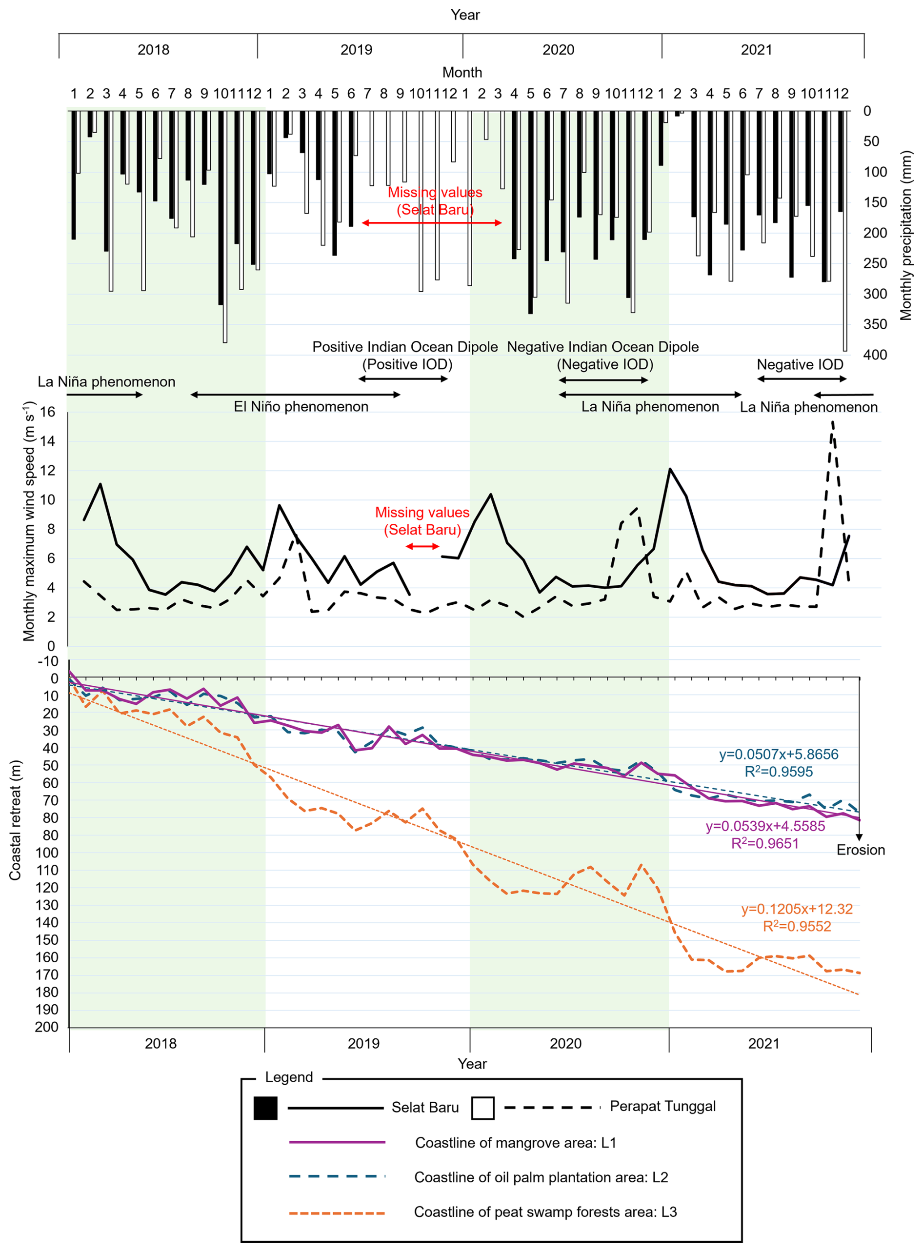
Figure 12Monthly precipitation (top) and monthly maximum wind speed (middle) at the Selat Baru and Perapat Tunggal stations on Bengkalis Island. Cumulative coastline retreat by land cover type from 2018 to 2021 based on Sentinel-1 data (bottom) are shown. The x-axis of the bottom figure represents the cumulative number of days since 1 January 2018 (where 1 January 2018 is day 0).
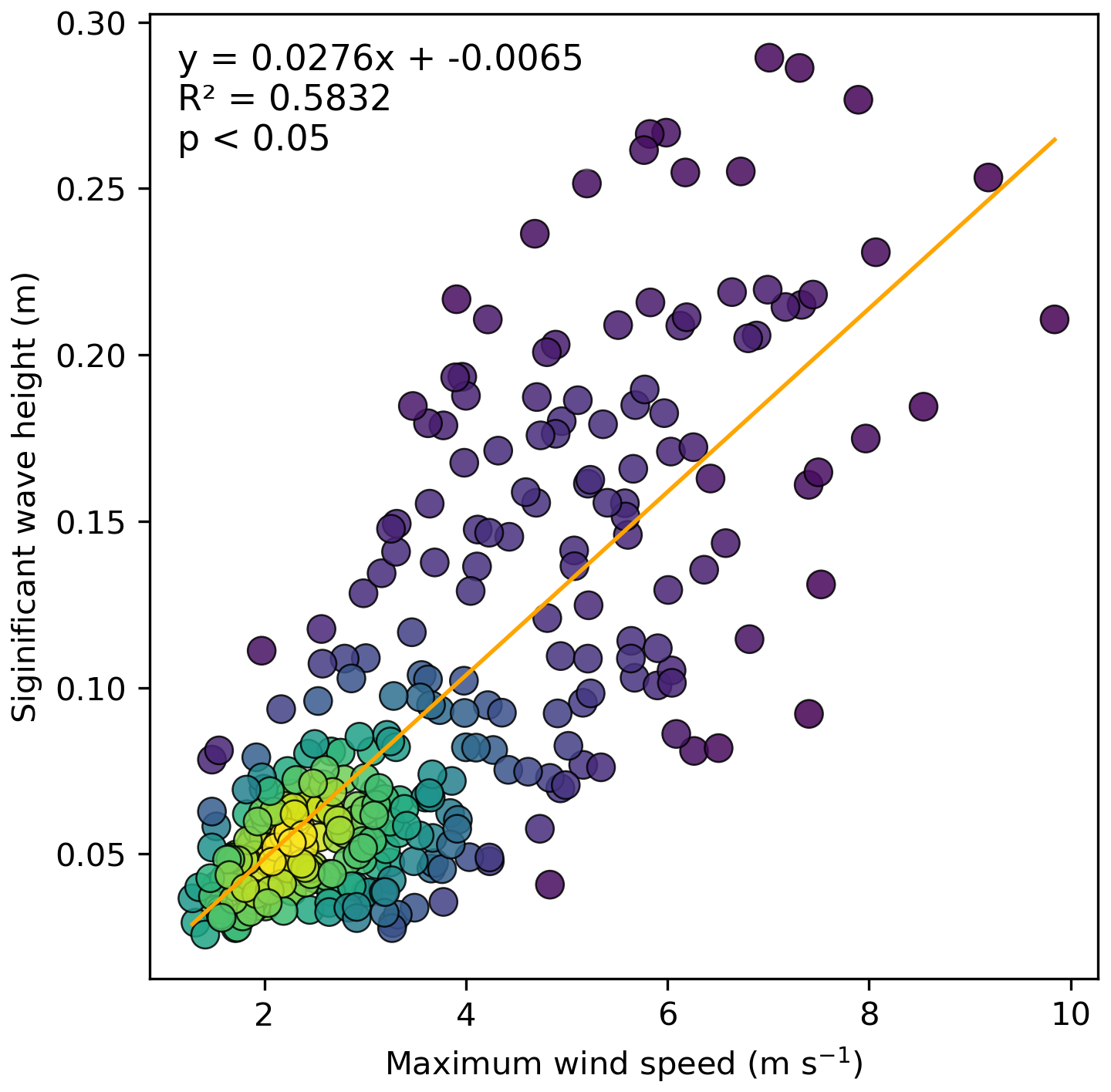
Figure 13Relationship between maximum wind speed and significant wave height at the offshore of the Bengkalis Island (St. M). A significant positive relationship (p<0.05, t-test) indicates that the regression is not a random coincidence.
Figure 13 illustrates the relationship between significant wave height and maximum wind speed, demonstrating that higher wind speeds correspond to greater significant wave heights.
Along the northern coast of Bengkalis Island, the lateral degradation of the mangrove areas has exposed the underlying peat substrate to coastal processes. Under the prevailing tidal and wave conditions, three types of erosion and progressive failure namely, toppling failure, rotational sliding, and cantilever failure have been documented (Basir et al., 2024). Consequently, during seasons characterized by dominant high wind speeds, increased wave heights may further accelerate coastal erosion.
4.4 Lateral degradation process of tropical peatland coasts
In tropical coastal areas, coastal erosion is accompanied by PMMs. A common characteristic of coastal land collapses is the spontaneous release of peat masses from the inland to coastal regions due to concentrated rainfall, which forms a peaty debris fan-shaped terrain. This article presents a one-year interval field observation study reporting the occurrence of a PMM event accompanied by coastal erosion. Figure 14 shows the annual changes in the area affected by landslides in the northwest area of Bengkalis Island. Following the PMM event, continuous coastal erosion resulted in traces of collapse. The land area initially increased after the PMM event but subsequently decreased during coastal erosion. Figure 14a shows a high-resolution satellite image (SPOT-6) captured on 18 September 2013, which depicts the state before the PMM event. At the concerned site, the southern part consists of an oil palm plantation, and the northern part consists of a peat swamp forest. Although the state of the PMM event after capture is uncertain, given the consistent coastal erosion in this area since 1972, according to Landsat images, coastal erosion could have occurred after the collapse. Figure 14b shows the area affected by the landslide after the PMM event photographed by UAV on 17 December 2014. Peat masses migrated from inland to the coast and formed a peaty debris fan. The fan extended offshore beyond the coastline on 18 September 2013. The area of the peaty debris fan formed is 0.80 ha. Further inland, pull-apart cracks were observed, which could have been caused by the gushing of peat toward the coast. From 18 September 2013, coastal erosion has continued in non-cracked coastal areas. This phenomenon indicates continued coastal erosion even before any coastal PMM event. Figure 14c shows the conditions captured by the UAV on 10 January 2015. A larger PMM event occurred on the western side of the coastal PMM event, as identified in the previous year. UAV observations resulted in the identification of a larger, peaty debris fan-shaped structure that was not confirmed on 17 December 2014. The structure of the peaty debris fan-shaped land formed by the movement of peat masses was observed to have changed, although no significant changes were observed in the PMM event on 17 December 2014. Figure 14d shows the UAV results from 5 March 2016. The peaty debris fan-shaped land caused by the large-scale PMM event in the west on 10 January 2015, had disappeared. The peaty debris fan-shaped land formed due to the PMM event on 17 December 2014, notably disappeared on 10 January 2015. Between 10 January 2015 and 5 March 2016, the peaty debris fan was gradually eroded from the east by waves (Fig. 14d). Figure 14e shows the UAV results for 4 March 2017. The peaty debris fan-shaped land that jutted out from the coastline on 18 September 2013, formed due to the PMM event on 17 December 2014, had completely disappeared by 4 March 2017, and the coastline retreated from its original position on 18 September 2013. Figure 14f shows the UAV results from 29 July 2018. The coastline has receded considerably since 18 September 2013, due to progressive coastal erosion. From 18 September 2013 to 29 July 2018, the coastline receded by approximately 90 m, averaging an annual retreat of approximately 18 m. As shown in this chapter, when a PMM event occurs in the coastal zone, a peaty debris fan is formed, leaving a collapse scar in the hinterland. The coastal erosion then proceeds until peat cliffs are formed.
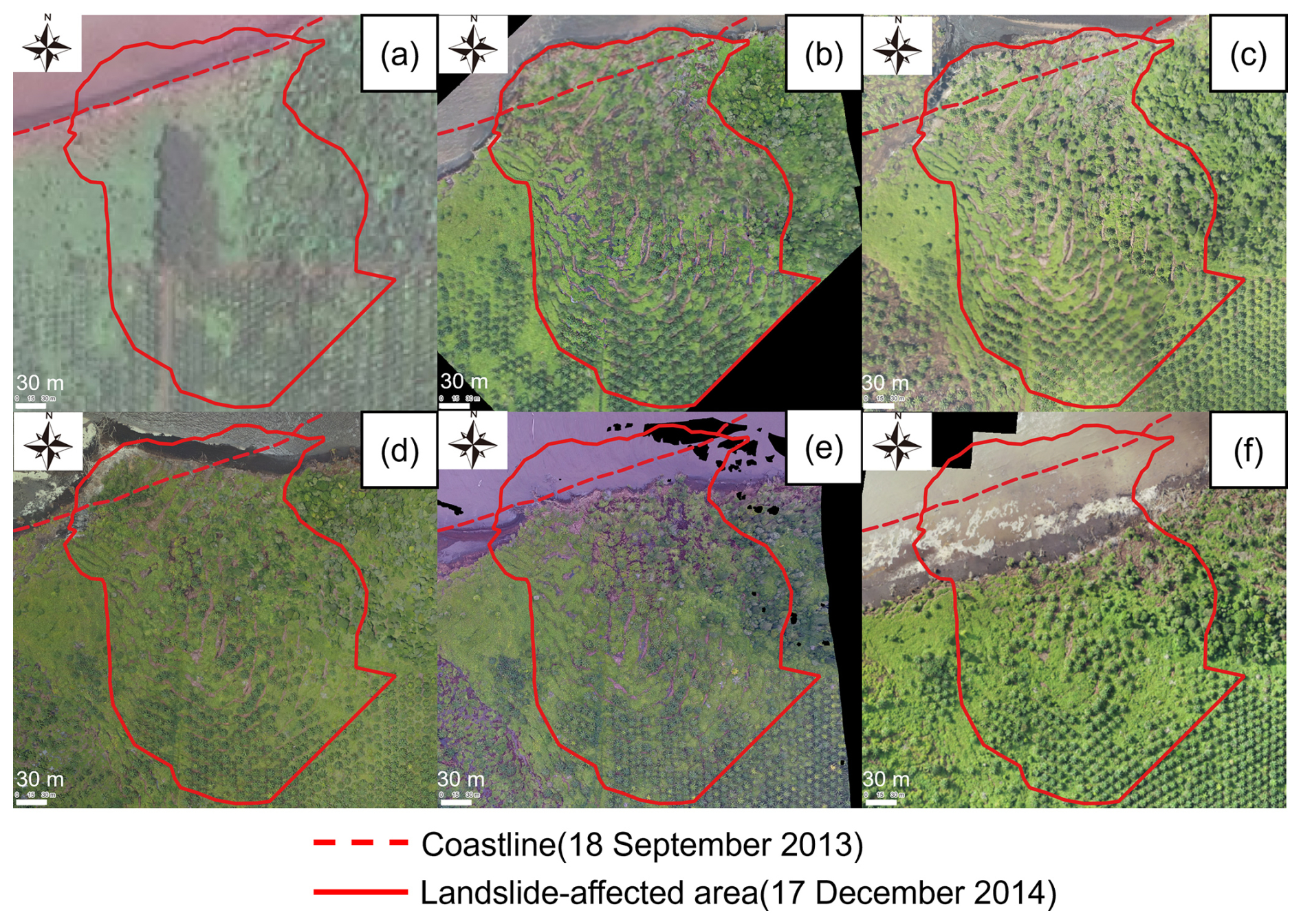
Figure 14Annual changes at the landslide-affected area in the northwestern part of Bengkalis Island. (a) Initial status of the focus area with a peat cliff coastline (SPOT-6, 18 September 2013). (b) The immediate aftermath of a peat mass movement; a peaty debris fan was confirmed outside the initial coastline, with many tears observed on the ground surface of the hinterland (UAV-based orthomosaic, 17 December 2014). (c) A larger peat mass movement occurred in the western area, creating a second peat fan, while the first peat fan remained (UAV-based orthomosaic, 10 January 2015). (d) The second peaty debris fan in the west area completely disappeared, while the first peaty debris fan remained (UAV-based orthomosaic, 5 March 2016). (e) Gradually, the first peaty debris fan eroded and decreased in area (UAV-based orthomosaic, 4 March 2017). (f) The first peaty debris fan disappeared, and the coastline receded approximately 90 m from the initial status on average, returning to a peat cliff (UAV-based orthomosaic, 29 July 2018).
Peat failures in boreal peatlands are known to cause substantial losses of peat and associated carbon (Evans and Warburton, 2007). When a landslide occurs, large volumes of organic-rich peat and mineral sediments are mobilized and transported downslope or into adjacent watercourses, resulting in significant carbon export from the peatland system. These failures therefore represent an important pathway for the removal and displacement of peat materials from the landscape.
Figure 15 summarizes the overall sequence of lateral degradation processes occurring along tropical peatland coasts. The process begins with the loss of mangrove belts, which reduces wave attenuation and promotes coastal erosion, ultimately leading to the formation of peat cliffs. Once a peat cliff develops, surface tearing at the head scarp can initiate a PMM, forming a peaty debris fan that extends seaward. Subsequent erosion of both the debris fan and the landslide-affected area results in the direct export of POC to the ocean (Yamamoto et al., 2019a). As erosion continues, the coastal peat cliff is gradually rebuilt, eventually allowing another PMM to occur and thereby completing a cyclic pattern of lateral degradation.
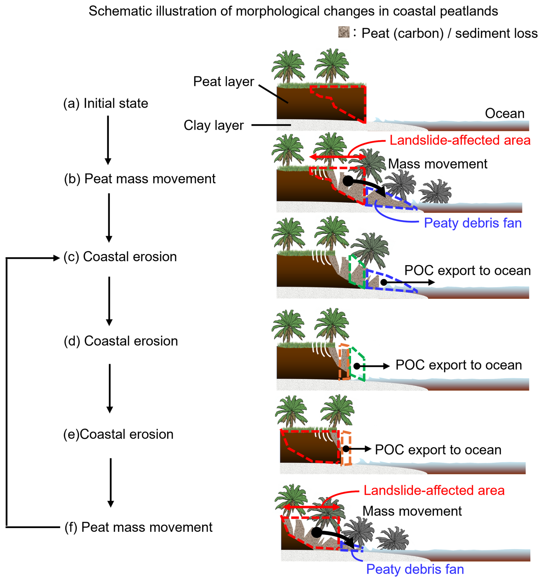
Figure 15Conceptual diagram illustrating the lateral degradation processes in tropical peatlands. (a) shows the conditions around the 1960s, when the loss of mangrove belts reduced wave attenuation and initiated coastal erosion, resulting in the formation of peat cliffs. (b) illustrates a peat mass movement (PMM) triggered at the head scarp, where surface tears developed and a peaty debris fan extended seaward. Subsequent stages (c)–(e) depict the progressive erosion of the debris fan and the landslide-affected area, leading to the direct export of particulate organic carbon (POC) to the ocean. (f) shows the stage at which the coastal peat cliff has been rebuilt by ongoing erosion, allowing a new PMM to occur and thereby completing the cyclic process of lateral degradation.
4.5 Analysis of soil sampling results: distribution of dry density, carbon density, and moisture content
Figure 16 shows the vertical distributions of dry density, carbon density, and moisture content. Under the groundwater level, a high moisture content, low dry density, and low carbon density were observed. High values of dry density and carbon density may have been observed on the surface of groundwater due to oxidative decomposition.
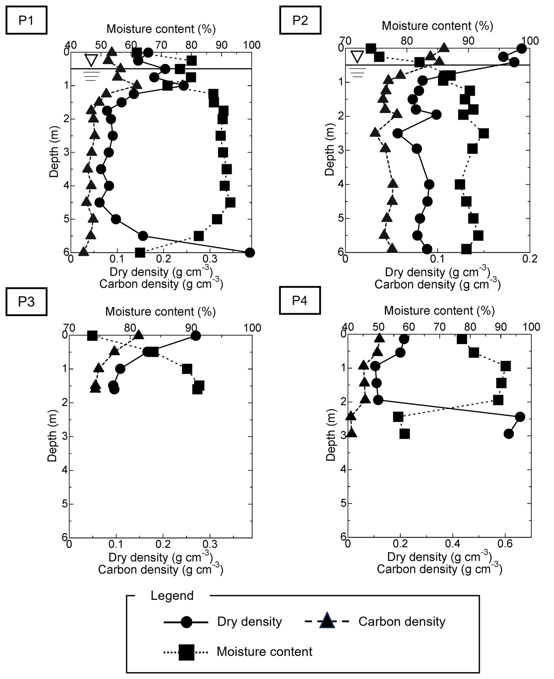
Figure 16Vertical distribution of dry density of peat, carbon density, and moisture content by peat core analysis in Bengkalis Island.
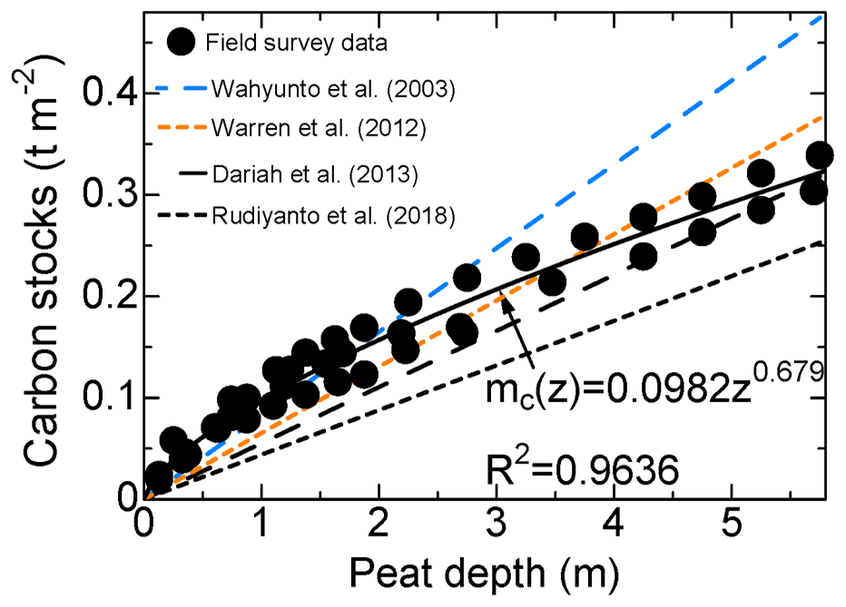
Figure 17Carbon stocks relative to depth. Literature values sourced from Wahyunto et al. (2003); Dariah et al. (2013); Warren et al. (2012) and Rudiyanto et al., 2018. The literature values from Wahyunto et al., 2003 were calculated using average values for the bulk density and carbon content of Hemic peat. Literature values from Dariah et al. (2013) were calculated using a function to estimate carbon stocks according to the depth of the peat layer. The literature values from Warren et al. (2012) were calculated using a function to estimate carbon stocks from average bulk density. Literature values from Rudiyanto et al. (2018) estimated carbon stocks from average carbon content and bulk density.
The accumulated organic carbon content was calculated vertically downward from the surface. The accumulated organic carbon content derived from the field survey results and literature values (Wahyunto et al., 2003; Dariah et al., 2013; Warren et al., 2012; Rudiyanto et al., 2018) is shown in Fig. 17. The accumulated organic carbon content was approximated by Eq. (15), using peat obtained from the field survey where mc(z) represents the carbon stocks (t m−2), and z represents the depth of the peat layer from the ground surface (m).
The results of peat sampling during the field survey could be approximated by the power approximation curve. The higher carbon stocks to a depth of 2 m is due to the groundwater table being present at a depth of 2 m, the environment being conducive to oxidative decomposition at the surface, and consolidation results in a higher bulk density. The outflow of particulate organic carbon into the sea due to coastal erosion and peatland degradation was estimated using the power approximation curve relationship described in this section.
4.6 Estimation of POC export to the ocean from lateral degradations
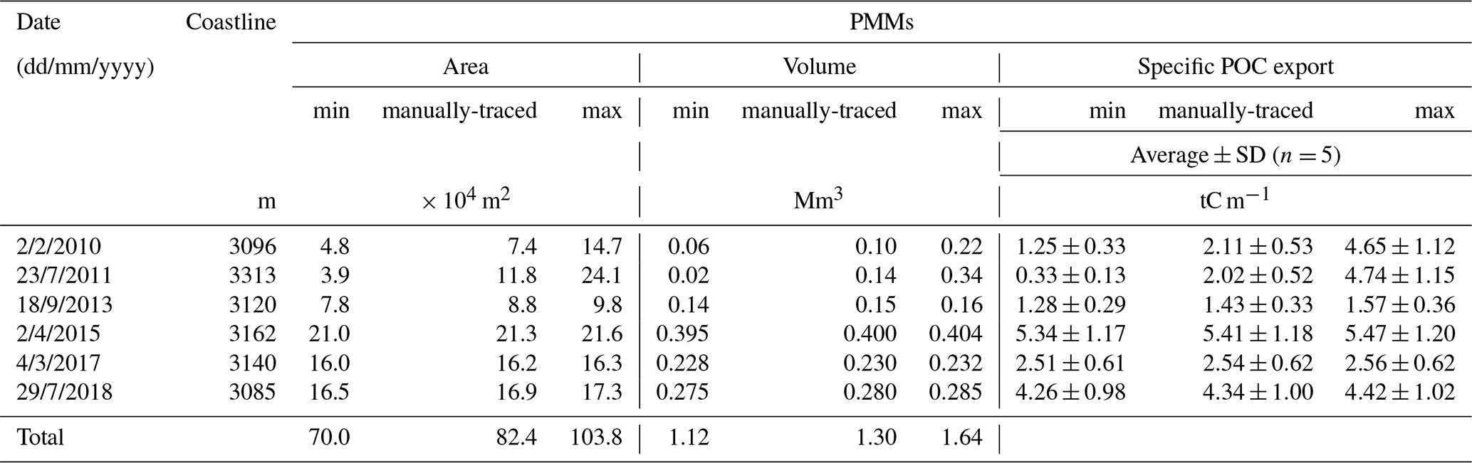
This study quantifies the export of POC to the ocean resulting from coastal erosion and PMMs. Figure 18 shows the annual changes in coastal erosion and landslide-affected areas. The estimated amounts of specific annual POC export to the ocean are shown in Fig. 19 and Tables 5 and 6. The average flux of POCs to the ocean due to coastal erosion along the study area of Bengkalis Island was estimated to be in the range of 2.06 to 7.60 tC m−1 yr−1. The average POC from the displacement of peat mass caused by PMMs was estimated to be in the range of 1.43 to 5.41 tC m−1, with an average increase of 2.23 tC m−1 from 2010 to 2018. In absolute terms, the mean POC export due to coastal erosion ranged from 6.46 to 24.03 ktC yr−1, while that associated with PMMs ranged from 4.45 to 17.10 ktC yr−1.
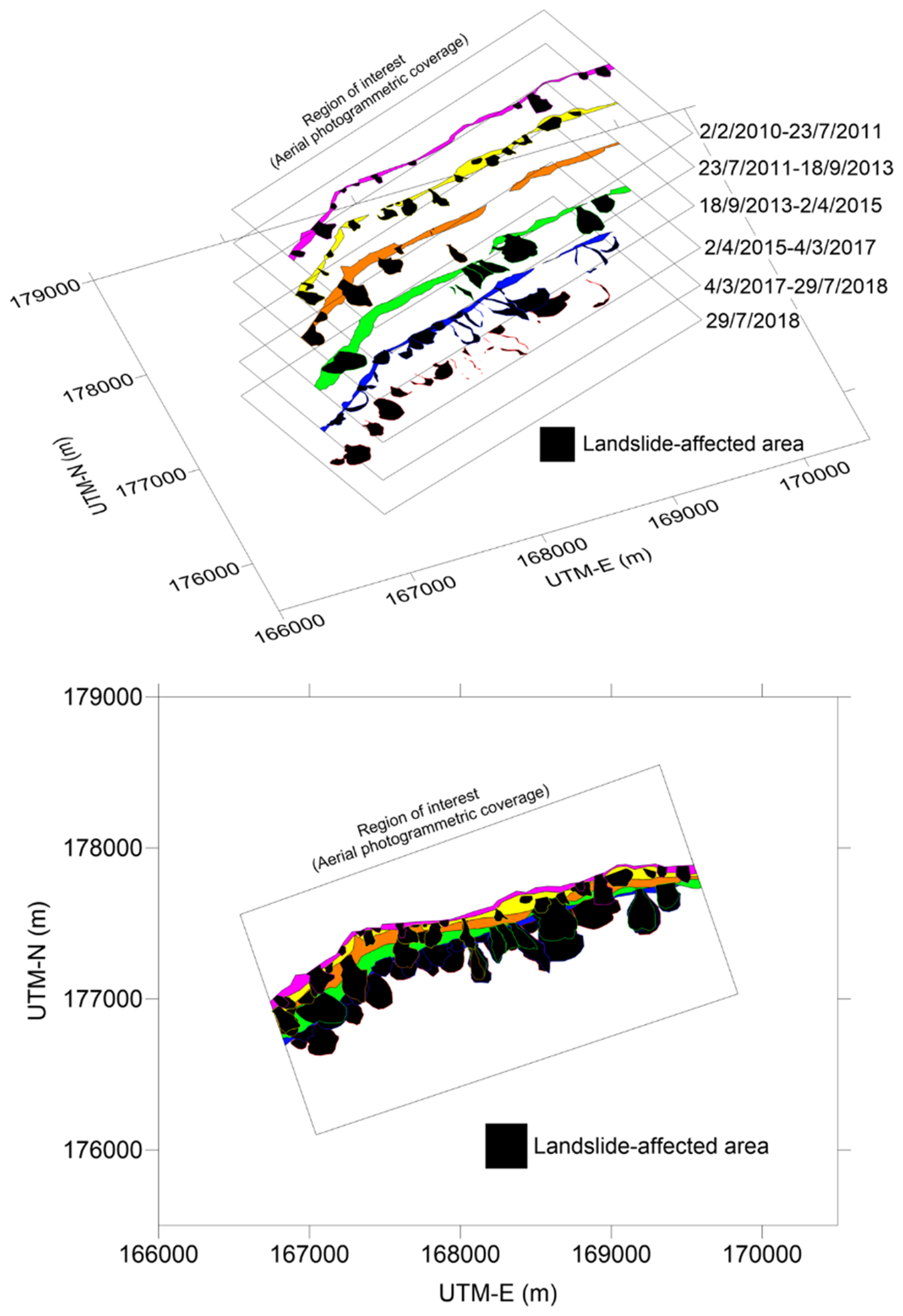
Figure 18History of coastal erosion and landslide-affected area within the region of interest (0.68 km2). This figure shows that the coastal erosion and peat mass movements occurred by turn and the landslide-affected area had been expanding towards the hinterland.
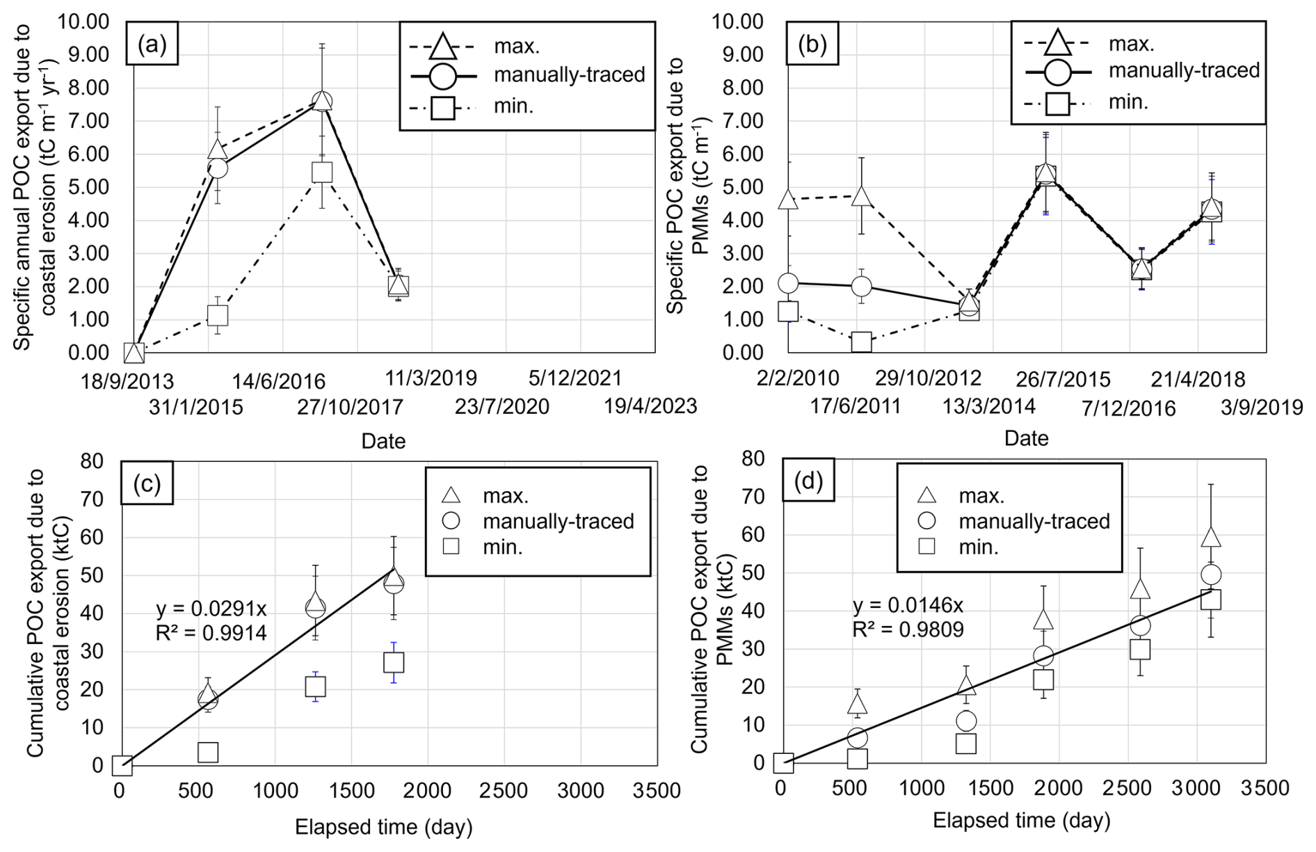
Figure 19Time series of (a) estimated specific annual POC export due to coastal erosion and (b) estimated POC export due to displacement of peat mass caused by PMMs for observation moment. The average specific annual POC export of POC to the ocean was estimated to be 2.06 to 7.60 tC m−1 yr−1 by coastal erosion and 1.43 to 5.41 tC m−1 from PMMs. The error bars indicate the standard deviation (SD). Panels (c) and (d) show the cumulative POC export derived from the time series in (a) and (b), indicating that the observed POC export is driven due to coastal erosion and PMMs.
Table 5The estimated volume of the eroded peat by the events of coastal erosion in each period. Changes in time in the estimated amount of POC from flows due to coastal erosion. SD indicates the standard deviation of the specific annual POC export calculated using the results of five patterns of carbon stocks calculations, including values from the literature. Where period (a) is 2 February 2010 to 23 July 2011, period (b) is 23 July 2011 to 18 September 2013, period (c) is 18 September 2013 to 2 April 2015, period (d) is 2 April 2015 to 4 March 2017 and period (e) is 4 March 2017 to 29 July 2018.
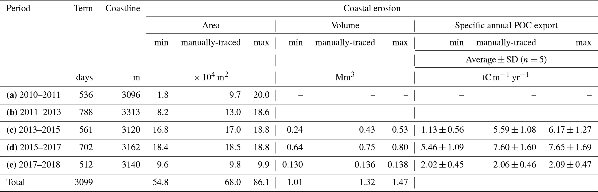
Table 6The landslide-affected area and the estimated volume of the eroded peat by the events of peat mass movements in each period. Changes in time in the estimated amount of POC from peat mass displacement caused by PMMs. SD indicates the standard deviation of the specific POC export calculated using the results of five patterns of carbon stocks calculations, including values from the literature.
Such fluxes, particularly from coastal erosion, far exceed those observed in natural river systems. The specific annual POC export due to coastal erosion in the studied catchment area (6.41 km2) was estimated at 1.01–3.74 ktC km−2 yr−1, which is up to 1089 times greater than the average POC export from tropical wet regions (0.00343 ktC km−2 yr−1; Ludwig et al., 1996). This underscores the significant role of coastal erosion in tropical peatland carbon dynamics.
In boreal peatlands, particulate organic carbon (POC) export has been attributed to gully erosion, with reported fluxes ranging from 0.0299 to 0.0319 ktC km−2 yr−1 (Evans and Lindsay, 2010). In comparison, the specific annual POC export associated with coastal erosion in the present study area is substantially higher, exceeding these boreal values by a factor of approximately 34 to 83. This contrast emphasizes both the spatial disparity in lateral carbon export and the underrecognized role of coastal erosion in tropical systems. Ongoing coastal erosion continuously discharges carbon into the ocean. On Bengkalis Island, 1 m of coastal erosion resulted in POC loss equivalent to annual CO2 emissions from 0.41–1.52 × 10⁴ m2 of degraded peatland (Hirano et al., 2014), underscoring the climate relevance of lateral specific annual POC export. The POC associated with PMMs was equivalent to emissions from 0.29–1.08 × 10⁴ m2 per metre of coastline. This indicates that coastal specific annual POC export may rival or surpass emissions from degraded inland peatlands. Tables 7 and 8 present the POC export associated with coastal erosion and peatland mass movements along a 3152 m coastline when converted to absolute terms. On a peatland coast with an average length of 3152 m, the estimated specific POC export to the ocean due to PMMs ranged from 5.07 to 7.02 ktC yr−1, while that from coastal erosion ranged from 6.46 to 24.03 ktC yr−1. Together, these processes constitute a dual mechanism of carbon loss that alters the carbon balance of tropical coastal peatlands.
Table 7The mean particulate organic carbon (POC) export attributable to coastal erosion ranged from 6.46 to 24.03 ktC yr−1 in absolute terms. Where period (a) is 2 February 2010 to 23 July 2011, period (b) is 23 July 2011 to 18 September 2013, period (c) is 18 September 2013 to 2 April 2015, period (d) is 2 April 2015 to 4 March 2017 and period (e) is 4 March 2017 to 29 July 2018.
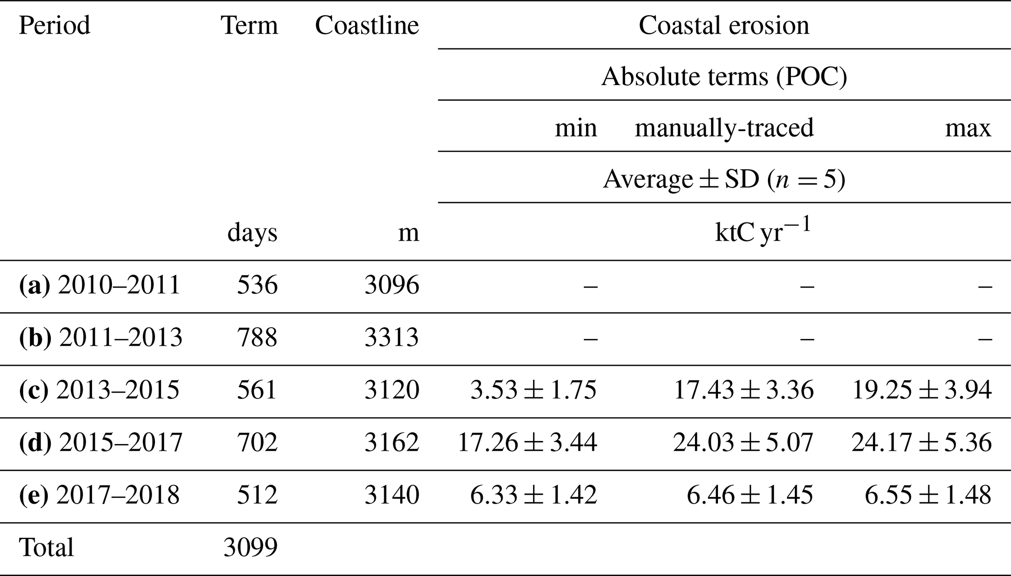
Table 8The mean particulate organic carbon (POC) export attributable to PMMs ranged from 4.45 to 17.10 ktC in absolute terms.
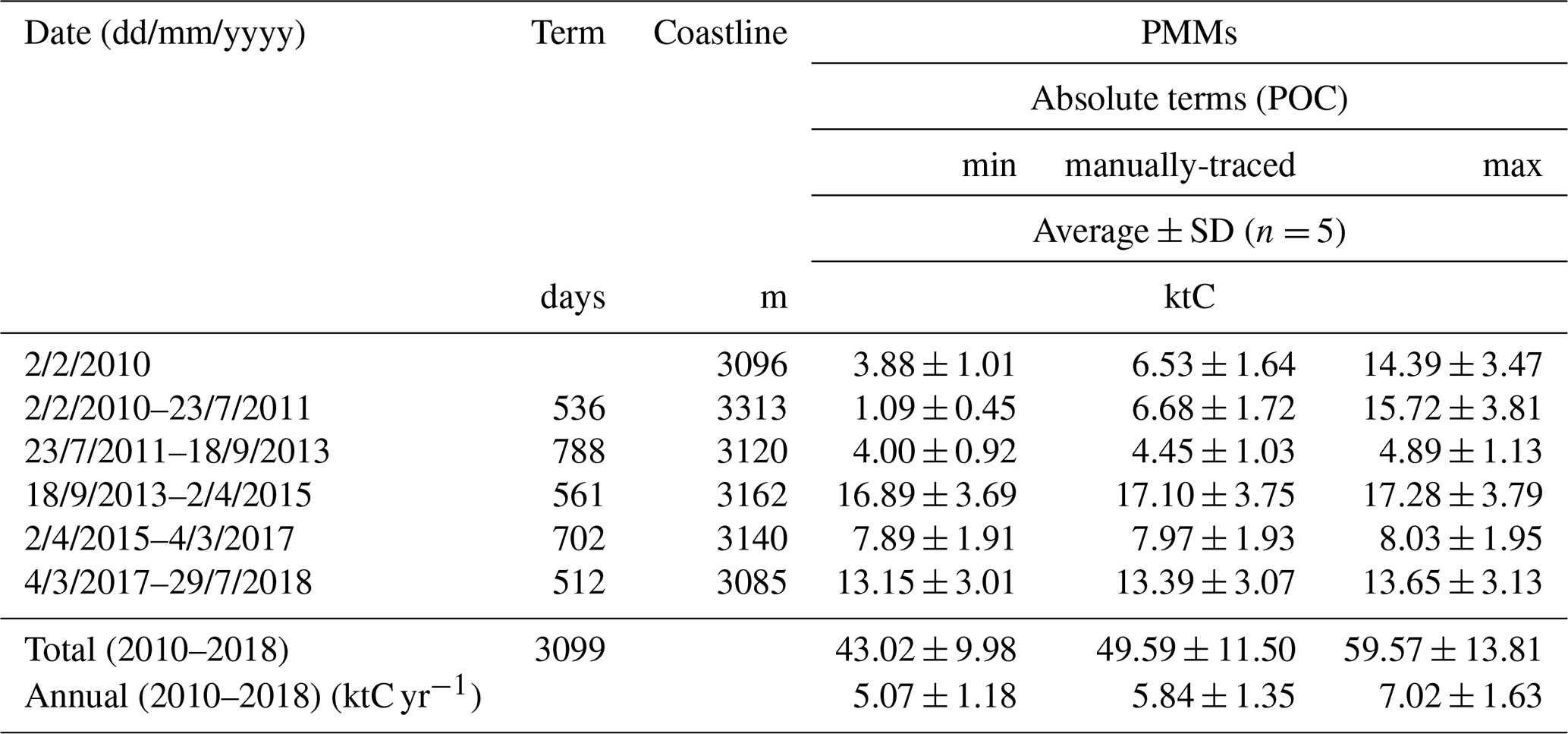
Figure 20 illustrates the fate pathways of particulate organic carbon (POC) exported from the northern coastal peatlands of Bengkalis Island, representing the source-to-sink or export processes toward the adjacent ocean. In summary, our results indicate that the coastal peatlands constitute the primary source of POC directly discharged into the Malacca Strait. Along a 3152 m coastline, coastal-erosion processes export an estimated 6.46–24.03 ktC yr−1, while peat mass movements (PMMs) contribute an additional 5.07–7.02 ktC yr−1 of POC to the Strait. Following its release, the exported POC may follow three possible fate pathways.
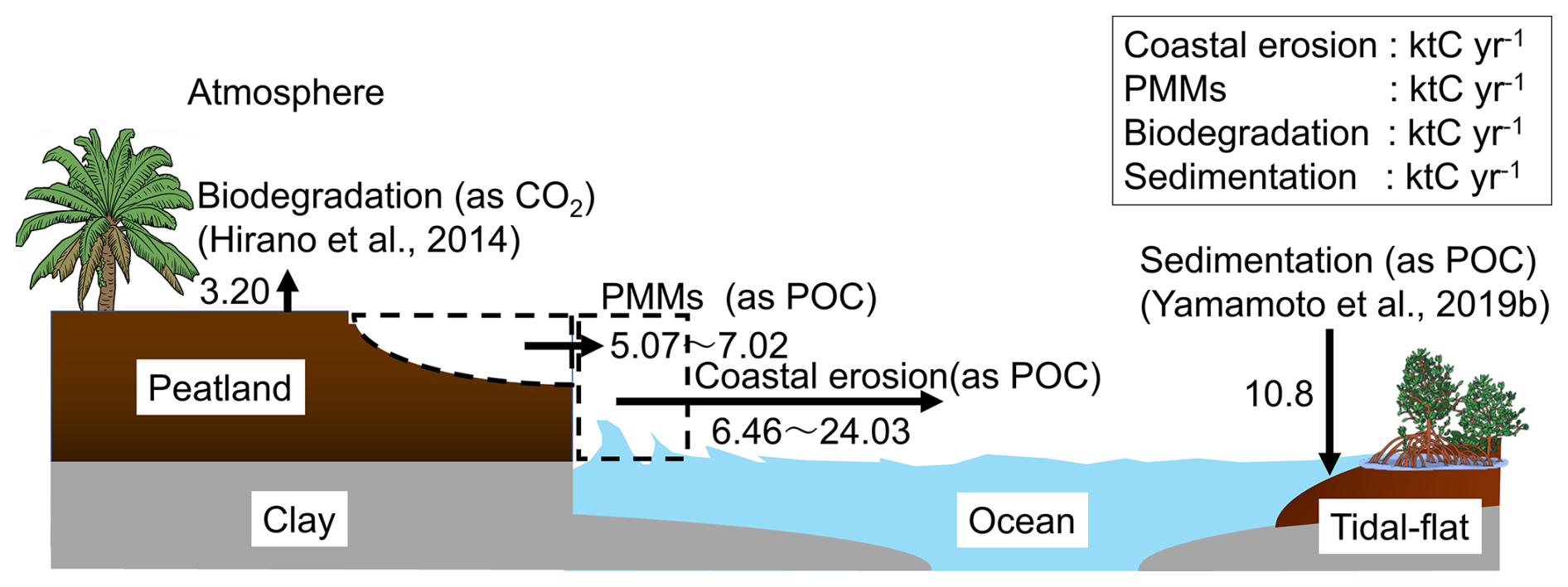
Figure 20Estimated annual particulate organic carbon (POC) flux around the studied peatland watershed (6.41 km2) in Bengkalis Island. Biodegradation was referred to Hirano et al. (2014). The coastline along the peatland watershed was 3.1 km and the area of the tidal flat in Bengkalis Island where the sedimentation happened was 1.46 km2.
First, a portion of the POC may remain suspended in the surface ocean or eventually settle on the seafloor, functioning as a long-term carbon sink. However, this pathway remains highly uncertain, and further investigation is required to constrain the magnitude and stability of this potential sink.
Second, as reported by Yamamoto et al. (2019b), part of the exported peat material may accumulate to form peat-derived tidal flat of 1.46 km2, where regenerated mangrove stands facilitate substantial carbon storage. Yamamoto et al. (2019b) estimated that such tidal flat can store approximately 10.8 ktC yr−1, suggesting that peat deposited in these environments may undergo reduced oxidative decomposition.
Third, peat-derived beach deposits (peat beaches) may develop along the coast, where enhanced microbial activity could accelerate peat decomposition, as suggested by Matsuo et al. (2025).
Collectively, these findings highlight that coastal peatlands act as major POC sources to the Strait of Malacca, while the subsequent carbon fate is partitioned among multiple pathways with varying degrees of uncertainty. Understanding the relative contributions of these pathways is essential for constraining regional carbon budgets and assessing the long-term implications of tropical peatland degradation.
Approximately 145 000 km2 of global tropical peatlands are located at or below 5 m elevation, making them vulnerable to future sea-level rise (Whittle and Gallego-Sala, 2016). Sea-level rise poses significant threats to low-lying tropical peatlands, particularly in Southeast Asia, including Kalimantan and Sumatra (Whittle and Gallego-Sala, 2016). In addition to sea-level rise, lateral degradation has also been observed across peatlands worldwide (Table B1 and Appendix A). Regarding coastal erosion, the coastline of the study area is retreating at 34 m yr−1 (Kagawa et al., 2017), which is dozens of times faster than erosion rates observed in boreal peatlands (The observed coastal erosion rates in boreal peatlands are 0.56–10 m yr−1; Appendix A). In addition to coastal erosion, PMMs represent another form of lateral degradation as shown in this study. Although erosion rates are particularly high here, sea facing peatlands globally may face similar threats. Furthermore, considering that peat decomposition leads to land subsidence, the situation becomes even more critical (Umarhadi et al., 2022). Considering the above situations, tropical peatlands are increasingly threatened by both lateral and vertical degradation processes. However, the fate of the exported peat remains unclear. Clarifying whether exported peat serves as a carbon sink or a source of carbon emissions is essential for understanding its role in the global carbon cycle.
This study is one of the first cases to quantify specific annual POC export from tropical coastal peatlands driven by both coastal erosion and PMMs. By combining erosion data with microbial and biochemical evidence from redeposition zones, this study provides a more comprehensive picture of lateral carbon dynamics in tropical coastal peatlands. These findings provide a foundation for incorporating coastal carbon export processes into peatland carbon budgets and highlight the urgency of protecting vulnerable shoreline peatlands from further degradation.
In this study, we have identified the conditions under which a chain of coastal erosion and peat mass movement events (PMMs) occur on tropical peatland islands with peat-formed coasts, and we have estimated the export of POCs to the ocean resulting from these processes. In coastal areas of tropical peatlands, coastal erosion promoted peat mass movements and vice versa. This chain of events of coastal erosion and peat mass movements proceeds as follows; When peat mass movement events first occur on a coastal peatland, peat is exported from the coast into the ocean, forming a peaty debris fan. Subsequent erosion causes the peaty debris fan to disappear, leaving the peat cliffs and the area affected by landslides. Long-term progression of coastal erosions has affected carbon export to marine environments from the peatland. The carbon export rate due to coastal erosion in the study watershed was estimated as 2.0–7.5 times higher than the carbon emissions due to biodegradation of peatland. The rates of coastal erosion were affected by the land cover. The coastal erosion rates of oil palm plantations exceeded those of mangrove or peat swamp forests by more than double. Strong winds correspond to high wave heights, emphasising the role of wind-induced wave activity in coastal processes, contribute significantly to the acceleration of coastal erosion.
PMMs also resulted in substantial peat loss and coastal geomorphic changes. Heavy precipitation played a crucial role in the triggering of PMMs. The carbon export rate through PMMs contributed to surplus carbon export, depending on the frequency of the PMMs. On a peatland coast with an average length of 3152 m, the amount of additional carbon export due to PMMs was estimated to range from 5.07–7.02 ktC yr−1, while it ranged from 6.35 to 23.9 ktC yr−1 due to coastal erosion. Compared to the typical specific annual POC export from tropical wet regions via riverine transport, these lateral carbon fluxes in this watershed (6.41 km2) correspond to approximately 295 to 1089 times greater. Consequently, these lateral carbon exports on tropical peatland coasts add another route for carbon export to the ocean, in addition to general POC discharges from rivers. Further studies need to clarify, the fate of exported peat particles in marine environments and emission of the carbon dioxide from exposed peat cliff formed by coastal erosion.
Peatlands are distributed across subarctic, arctic, and tropical regions (Fig. A1). Throughout the Holocene, they have functioned as persistent carbon sinks. Globally, peatlands are estimated to have sequestered more than 600 GtC at a rate exceeding 5 GtC per century (Kleinen et al., 2010; Yu, 2011).
The total peatland area is estimated to range from 3.97 to 4.26 million km2, accounting for approximately 3.05 % to 3.28 % of the Earth's land surface (Osaki and Tsuji, 2016; Ministry of the Environment, 2002). Despite this limited spatial extent, peatlands are estimated to store about 6 % of the global soil carbon stock (Page et al., 2011; Scharlemann et al., 2014).
-
Bykovsky Peninsula, Siberia (Fig. A1a)
Annual erosion rates vary significantly on interannual and decadal scales (Lantuit et al., 2011). Sediment accumulation can reach 5.00 m yr−1, with coastal retreat rates up to 10.00 m yr−1. From 1986–2006, the average erosion rate was 1.09 m yr−1, with a peak of 2.06 m yr−1 from 1975–1981. Storms (≥10 m s−1 for ≥ 6 h) occurred on average 13.6 times per year between 1958 and 2006, but erosion did not correlate directly with storm frequency due to a “lag effect” (Lantuit and Pollard, 2008).
-
Beaufort Sea Coastline (Fig. A1b)
Yunker et al. (1991) divided the coastline from Cape Dalhousie to the Alaska border into 776 segments, calculating coastal retreat and estimating peat flux into the sea by multiplying retreat rates with peat thickness.
-
Elson Lagoon, Alaska (Fig. A1c)
From 1949 to 2000, retreat rates increased from 0.56 m yr−1 (1948–1979) to 0.86 m yr−1 (1979–2000), resulting in a 47 % increase and 2.8 × 10⁵ m2 land loss. Erosion is restricted to the ice-free season (3–4 months yr−1). Regional retreat rates range from 2 to 6 m yr−1, with maxima exceeding 10 m yr−1 (Rachold et al., 2002).
-
Baltic Sea Coastal Peatlands (Fig. A1d)
Coastal low-lying peatlands cover ∼0.16–0.2 km2 (Lehfeldt and Milbradt, 2000). Coastal erosion and storm abrasion have exposed peat layers by removing overlying sand. Saltwater intrusion affects ∼ 1800 km2 of wetlands (Sterr, 2008), and ∼3 km of wetland has been lost in the southern Baltic Sea since peat formation began. Coastal wetlands face multiple stressors, including sea-level rise, flooding, submergence, and infrastructure restrictions on inland migration (Nicholls and Cazenave, 2010; Wong et al., 2014; Chambers et al., 2019).
-
Amazonian Peatlands and Coastal Erosion (Fig. A1e)
Research in Amazonian peatlands began in the 1950s and has expanded significantly since 2009, shifting from carbon dynamics to degradation and conservation (Malpica-Piñeros et al., 2024). The Amazon Basin spans nine countries, with most peatland studies concentrated in Peru. High-altitude peatlands are found in the Andes, Guiana Shield, and Brazilian Shield. In Guiana, coastal erosion such as beach retreat has been observed (Chevallier et al., 2023).
-
Boreal Peatlands and Peatland Failures (Fig. A1f)
Peat mass movements (PMMs) in boreal regions include bog bursts, bog slides, and peat flows (Dykes and Warburton, 2007). Common triggers include heavy rainfall, drainage, and snowmelt. Failures have been documented since the 16th century in northern England and Ireland (e.g., Bowes, 1960; Warburton et al., 2004; Dykes and Jennings, 2011). Most failures occur on 2–3 m thick peat over slopes of 4–8°, but steeper failures also occur. Consequences include fish kills (McCahon et al., 1987) and drainage disruptions (Alexander et al., 1986).
-
Coastal Wetland Vulnerability and Degradation (Fig. A1g)
According to Chambers et al. (2019), low-lying coastal wetlands are undergoing degradation due to combined climatic and anthropogenic stressors, resulting in reduced ecological health and shrinking spatial extent. These wetlands, located within the intertidal ecotone between marine and terrestrial environments, face multi-directional threats.
-
Tropical Peatland Failures (Fig. A1h)
Documented cases of PMMs in tropical peatlands are rare. The only known cases include: A suspected landslide on the Tutoh River, Malaysia in 1966 (Wilford, 1966).
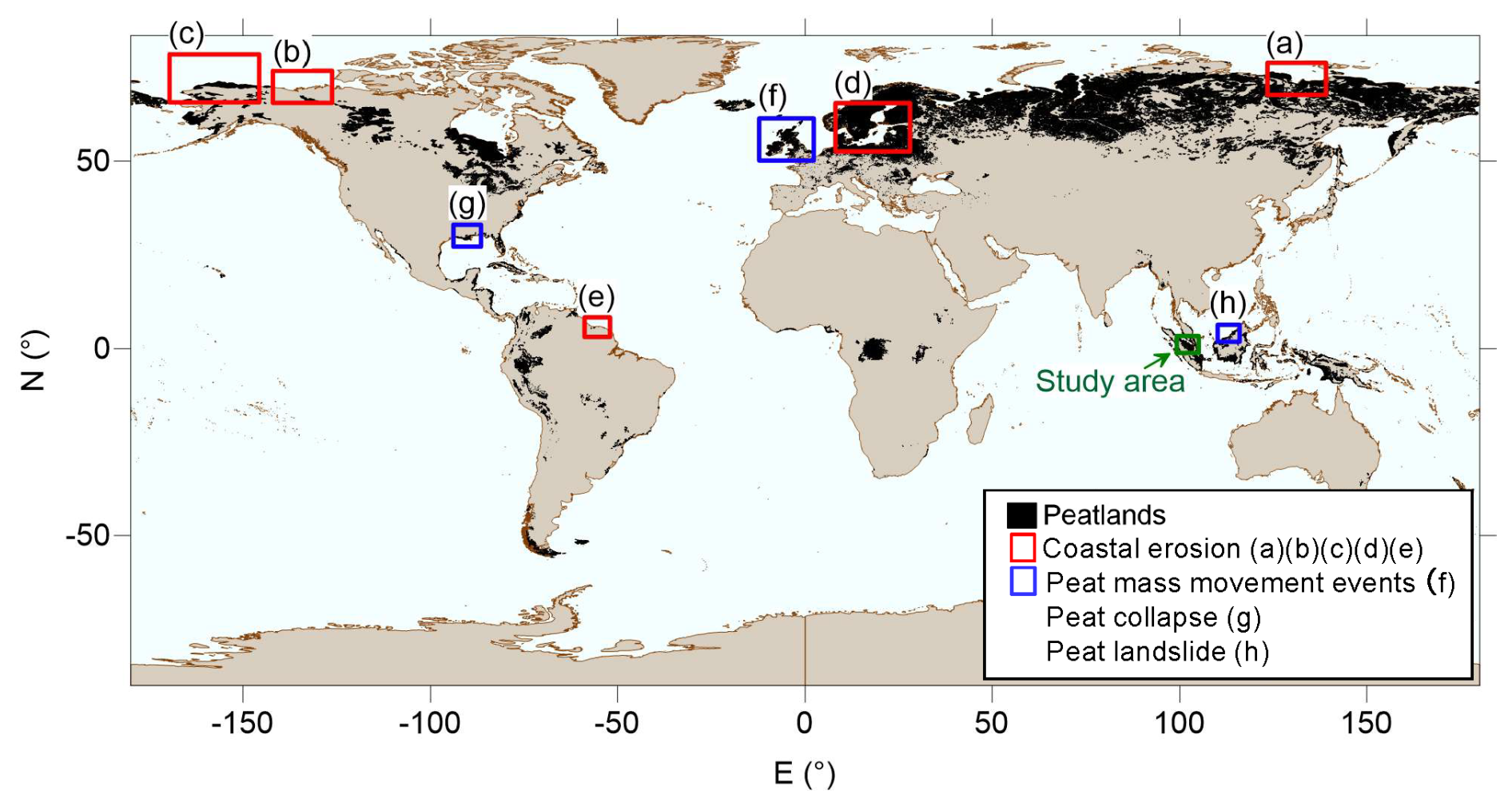
Figure A1Global distribution of the lateral degradation in peatlands (Based on data from the Global Peatland Database, compiled by the Greifswald Mire Centre (2024)).
Table B1 provides an overview of previous studies reporting carbon emissions from peat and peatland systems in boreal and tropical environments.
Table B1Comparison of carbon export studies in Boreal and Tropical peatlands.
EO Browser was utilized as a web-based platform for processing remote sensing data in a cloud computing environment. Sentinel images were obtained from Sentinel Hub, which is connected to EO Browser via API, and statistical analysis of the Normalized Difference Vegetation Index (NDVI) was conducted within EO Browser. The procedure for NDVI statistical analysis in EO Browser is as follows: First, the acquisition period for the Sentinel images was selected, and polygons from a KML file created in a GIS environment were imported into EO Browser. The statistical analysis of NDVI allowed for the calculation of average values within the selected polygons and the assessment of temporal changes over the specified period. To minimize the impact of cloud cover, the analysis was conducted with cloud coverage set to 0 %. Since erroneous data were occasionally included, the exported CSV files were reviewed, and any erroneous data were manually removed.
Time-series changes in NDVI were analysed using Landsat8, while Sentinel-2 imagery was employed to examine the relationship between NDVI and vegetation cover. Consequently, we first established the relationship between NDVI values from Landsat8 and Sentinel-2.
Landsat 8 OLI images from 9 March 2017 to 19 February 2022 were used. The target site is indicated in Fig. 3c (ROI1). Landsat 8 was launched in 2013 and provides high-quality multispectral images at a resolution of 30 m and a revisiting time of 16 d.
Sentinel-2 multispectral imagery captured on 22 March 2017, was used for land cover classification. Sentinel-2B provides 13 bands of multispectral imaging at a resolution of 10 m. Sentinel-2B was launched on 7 March 2017. Part of a European fleet of satellites aimed at delivering core data to the European Commission's Copernicus programme, a programme whose services address six thematic areas: land, marine, atmospheric, climate change, emergency management, and security. In a sun-synchronous orbit at a mean altitude of 786 km above the Earth's surface, MSI samples 13 spectral bands in the visible-near infrared (VNIR) and short-wave infrared (SWIR) spectral range at three different spatial resolutions (10, 20, and 60 m) and allows for a 290 km swath width with a high revisit frequency of 10 d. Data were obtained from USGS EarthExplorer (https://earthexplorer.usgs.gov/).
An oil palm plantation was selected as the target for comparison (Fig. 3c (ROI2)). To determine whether NDVI variation is related to vegetation coverage, VARI (Visible Atmospherically Resistant Index) images were generated from UAV aerial photogrammetric data acquired on 4 March 2017. The VARI images were binarized using a threshold of 0, and a scatter diagram was constructed to compare the binarized VARI values with the NDVI data. Pixel sizes were matched to facilitate the correlation analysis between vegetation coverage and NDVI. NDVI (Landsat 8), NDVI (Sentinel-2) and VARI were calculated using Eq. (D1), Eq. (D2) and Eq. (D3).
where B5 represents the NIR with 30 m resolution (wavelength: 850–880 nm); B4 represents the red band with 30 m resolution (wavelength: 640–670 nm); B8 represents the NIR with 10 m resolution (wavelength: 842 nm); B4 represents the red band with 10 m resolution (wavelength: 665 nm). G stands for the green band; R stands for the red band; B stands for the blue band.
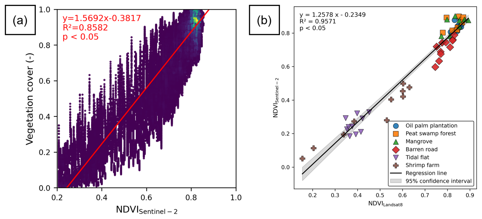
Figure D1(a) Relationship between Sentinel-2 NDVI and vegetation cover. (b) Relationship between Landsat 8 NDVI and Sentinel-2 NDVI, and Both figures show a linear relationship. A significant positive relationship (p<0.05, t-test) indicates that the regression is not a random coincidence.
Changes in NDVI and vegetation cover were plotted as a time series to highlight where the vegetation became discontinuous. Figure D1a illustrates the relationship between vegetation cover and NDVI which exhibits a clear correlation, as expressed by Eq. (D4) (with VC representing vegetation cover and NDVISentinel-2representing NDVI of Sentinel-2). Additionally, a strong correlation was observed between the NDVI values from Landsat 8 and Sentinel-2; this relationship is shown in Fig. D1b and expressed by Eq. (D5), where x is the NDVILandsat8 from Landsat 8 and NDVISentinel-2 is that from Sentinel-2.
To extract bare land from oil palm plantations in satellite images, we used the normalised difference vegetation index (NDVI), and the normalised difference moisture index (NDMI) derived from Sentinel-2 imagery to classify the land cover. NDVI and NDMI were calculated using Eqs. (D2) and (E1), respectively. For machine learning, Support Vector Machine (SVM) algorithms were used to classify the oil palm tree plantations from the other landcovers. The UAV images, taken on 4 March 2017, 29 July 2018, and 5 November 2019, were used as the ground truth of the land cover. The precision of the land cover classification was evaluated by calculating the true positive rate, recall, specificity, precision, negative predictive value and F-score based on the confusion matrix. The dividing lines were calculated with palm oil plantation vegetation as true positives (TP) and other types of land cover as false negatives (FN).
where B8A represents the NIR with 20 m resolution (wavelength: 865 nm); B11 represents the SWIR with 20 m resolution (wavelength: 1610 nm). According to Mandanici and Bitelli (2016), the Pearson correlation coefficient and the slope of the linear relationship between the reflectance and index values of the multispectral instrument (MSI) and the TM5 bands are as close to 1 as possible, with the intercept close to 0. Therefore, the machine learning model for land cover classification created for Sentinel-2 images was applied directly to Landsat5 images.
As a result of the machine learning of the landcover classification using NDVI and NDMI, we got the partition line separating vegetation area and bare land area given by Eq. (E2). Validation results of the machine learning were as follows: true positive rate, 0.8804; recall, 0.6940; specificity, 0.9950; precision, 0.9885; negative predictive value, 0.8410; and F-score, 0.4077.
Because DEMNAS is a DSM that contains the tree height (vegetation), we removed the tree height from the DSM to make DTM. First, the bare lands in the research area in Landsat 5 image taken on 2 February 2010 were identified by the classifier that was established in 3.2.1 and binarized. The binarized bare land area and DEMNAS data were combined to extract elevation values for bare land. During this process, the peat swamp forest and adjacent bare road and a radius of 200 m from the coastline that were flagged as anomalies were masked (Fig. F1a). The 200 m radius DEMNAS data depicted collapsed terrain, which would not need to remove tree heights; therefore, these areas were excised. The DEMNAS derived coastline, which the points of the altitudes of 0 m at 100 m intervals were extracted (Fig. F1b). An approximation of the polynomial curve of the extracted coastline was calculated, and a 2 km offshore measurement line was constructed centred on the coast (Fig. F1c). The radius of 1 km from the coastline was set as a buffer area for buffer analyses in GIS to obtain elevation of the bare land (Fig. F1d and F1e). For any point in which statistical values were not attainable, linear interpolation was applied between adjacent points. The elevation difference from the median bare land elevation was considered as tree heights and the difference was subtracted to calculate the bare land elevation. Values above 0 m elevation were used to interpolate by kriging to generate a DTM with an 8 m resolution.
Figure F2 shows the differences in the DEMNAS before and after vegetation removal. The median elevation values of the bare land within 1 km from coastline were used in the vegetation removal from the DEMNAS data. Comparison between ground surface geodetic survey results by Real Time Kinematic-Global Navigation Satellite System (RTK-GNSS) and DEMNAS data after vegetation removal are presented in Fig. F3. The RMSE of the ground elevation obtained from the RTK-GNSS and DEMNAS data after vegetation removal was 0.6951 m. The RMSE was subtracted from the DSM obtained from the UAV aerial photogrammetry to match the DEMNAS elevation. This elevation difference can be caused by the skewness by the elevation decline because of the waterway.
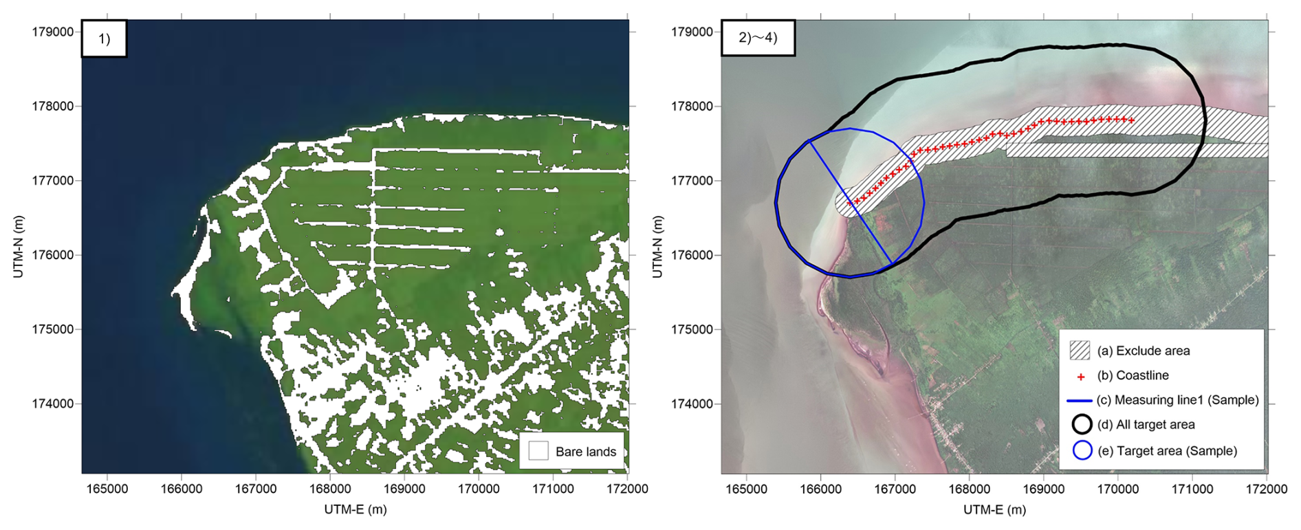
Figure F1Methodology of removal of vegetation from DEMNAS data. (1) A Landsat5 image (2 February 2010) was used to classify bare land and other land covers using machine learning. (2) The bare land raster was set at 1 and multiplied by the DEMNAS data to produce the bare land elevation data. The elevation anomalies at the boundary between the peat swamp forest and the bare road and a radius of 200 m from the coastline (a) were masked. (3) A measuring line was made in the offshore direction from inland at points where the coastline was divided at 100 m intervals (b) and (c). (4) The median elevation of the bare lands found 1 km (d) and (e) from the coastline was assigned to the coastline and linearly complemented.
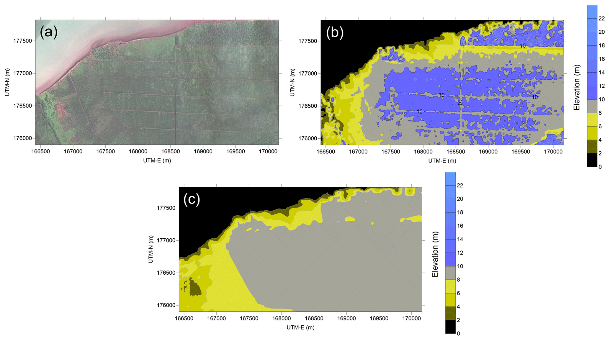
Figure F2Comparison of (a) SPOT-6 data with (b) original DEMNAS data with (c) DTM removed from vegetation. The elevation of the bare land above 0 m was used to interpolate and generate a DTM with an 8 m resolution by kriging. Satellite imagery (a: SPOT-6) and topographic data (b: DEMNAS) are ©Airbus DS/Spot Image and Badan Informasi Geospasial (BIG), respectively.
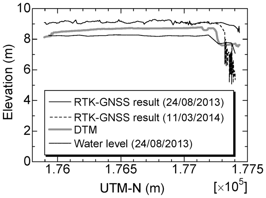
Figure F3Comparison of the RTK-GNSS land survey with a section created from DEMNAS data. The section where the elevations of DTM has decreased was the section where the collapse was identified in December 2013 after the RTK-GNSS land survey. The RMSE of removing the landslide-affected area was 0.6951 (m).
In this study, optical satellite imagery and UAV-based orthomosaic were used to identify landslide-affected areas and coastlines. A comparison of Landsat8 imagery, which has a resolution equivalent to Landsat5, the lowest resolution of the optical satellites used, and UAV-based orthomosaic Landslide-affected areas at the same location is shown (Fig. G1a, G1b, G1c, G1d and G1e; described in Sect. 3.2.4 and 3.2.6). Errors due to tracing were considered to vary depending on the resolution of the imagery, such as low-resolution satellite imagery, high-resolution satellite imagery and UAV-based orthomosaic, as the landslide-affected area and coastline cannot be identified unless the zoom is adjusted so that a wide area is visible, depending on the resolution of the imagery (Fig. G1a, G1b, G1c, G1d and G1e; described in Sect. 3.2.4 and 3.2.6). The process in GIS software of estimated the volume of peat exported to the ocean is shown (Fig. G1e, G1f, G1g, G1h, and G1i; described in Sect. 3.2.3).
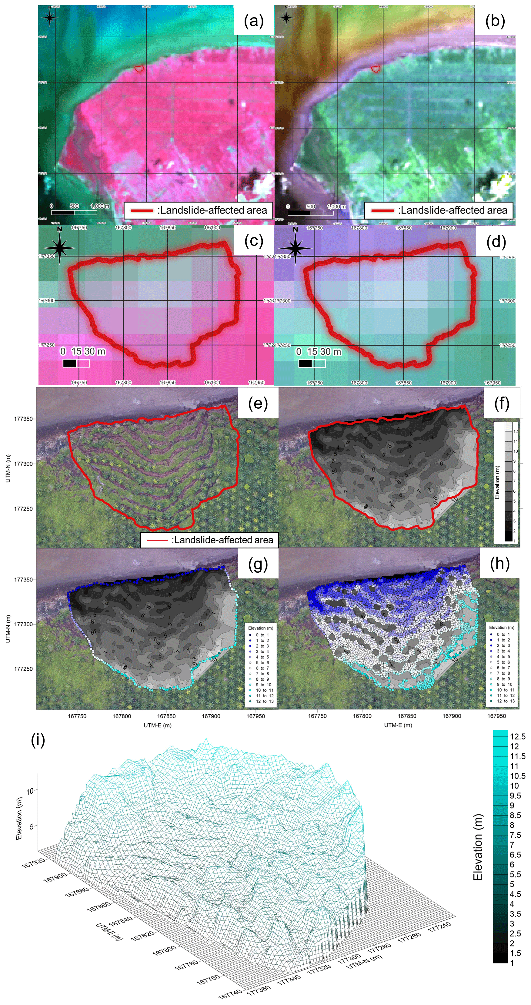
Figure G1Comparison of optical satellite images and UAV-based orthomosaic and the process in GIS software of estimating the volume of peat exported to the ocean. (a) Landslide-affected area identified by wide-area visibility and UAV-based orthomosaic (4 March 2017) in Landsat 8 false colour image (9 March 2017). (b) Landslide-affected area identified by wide-area visibility and UAV- based orthomosaic (4 March 2017) in Landsat 8 true colour image (9 March 2017). (c) Landslide-affected area identified by zoomed-area visibility and UAV-based orthomosaic (4 March 2017) in Landsat 8 false colour image (9 March 2017). (d) Landslide-affected area identified by zoomed-area visibility and UAV-based orthomosaic (4 March 2017) in Landsat 8 true colour image (9 March 2017). (e) Landslide-affected area identified by UAV-based orthomosaic (4 March 2017). (f) DEM was post-collapse DEM, which were generated by sampling elevation data in the landslide-affected areas of vegetation removed DSM.(g) Elevation points at the edge of the DSM of the landslide affected area extracted to recreate the initial land surface. (h) Elevation points (4516 points) inside the DSM of the landslide-affected area extracted to recreate the DEM after collapse. (i) Shape of the collapse site with the vegetation removed.
This study considered traced errors in coastal erosion areas and landslide-affected areas, which were calculated by manual tracing in GIS software. The concept of an error evaluation method for traced coastal erosion areas and landslide-affected areas on GIS software is presented in Fig. H1. When considered at the scale of one pixel in the image, it was assumed that the manually traced lines would have trace errors within one pixel. Therefore, the traced error will depend on the resolution. Here, for the case where Google Earth was used, it was assumed that a tracing error equivalent to that of Landsat5 would occur, as the resolution was not opened. For cases where low-resolution images are used, the tracing errors are greater because the landslide-affected area and the coastline cannot be identified without scaling the scale (Fig. G1a, G1b, G1c, G1d and G1e). Errors in tracing planes also affect the calculation of volumes. Traced errors were also reflected in volume calculations.
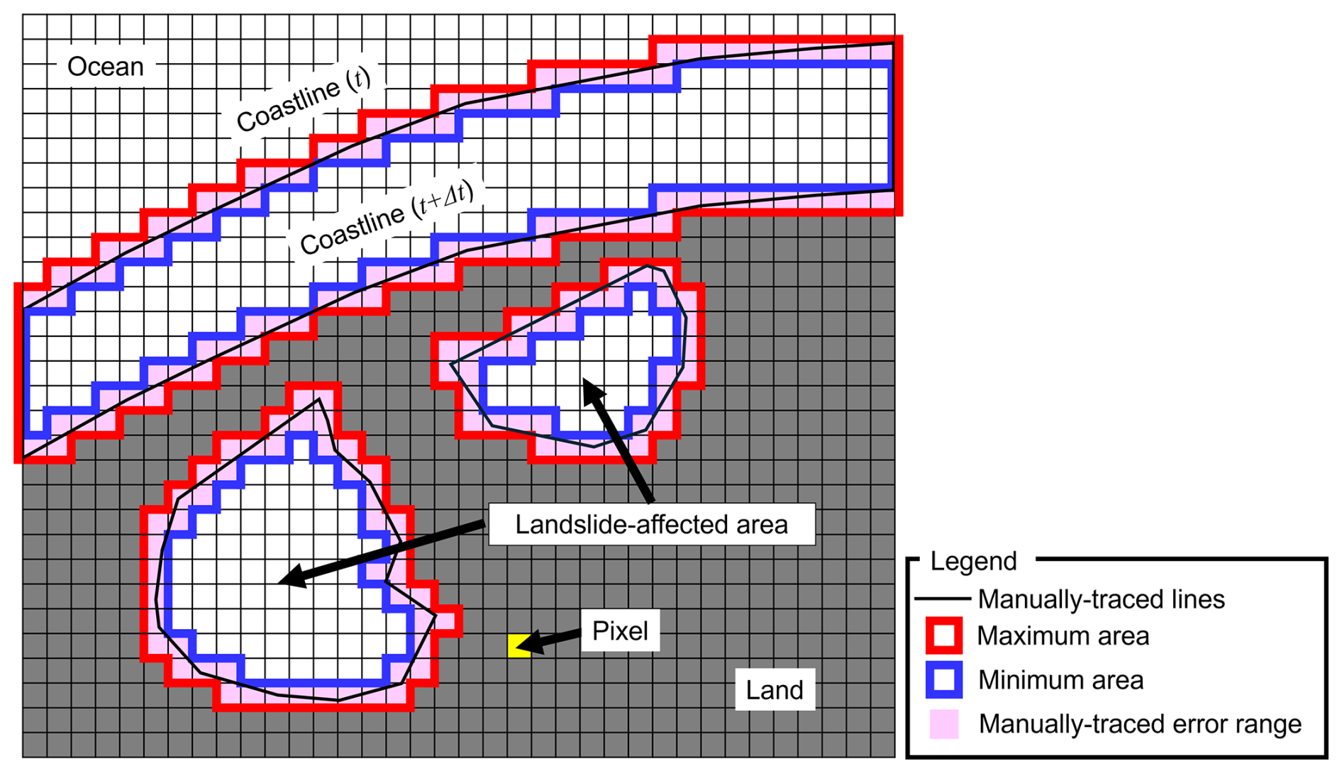
Figure H1Concept of the error evaluation method for traced coastal erosion areas and landslide-affected areas in the GIS software. Manual tracing errors tend to be resolution dependent.
We evaluated the errors caused by differences in resolution using satellite images from Landsat 8 and Sentinel-2 acquired at the same time (n= 7). To achieve this, we conducted 20 tracings per time for comparison. Using Landsat 8 with a 30 m resolution and Sentinel-2 with a 10 m resolution, landslide-affected areas captured at the same time were manually traced, and the error was evaluated (Fig. I1). Larger collapses exhibited greater tracing errors, with an overall RMSE of 0.608 × 10⁴ m2 the results also indicate that tracing variability is greater with Landsat 8, which has a lower resolution.
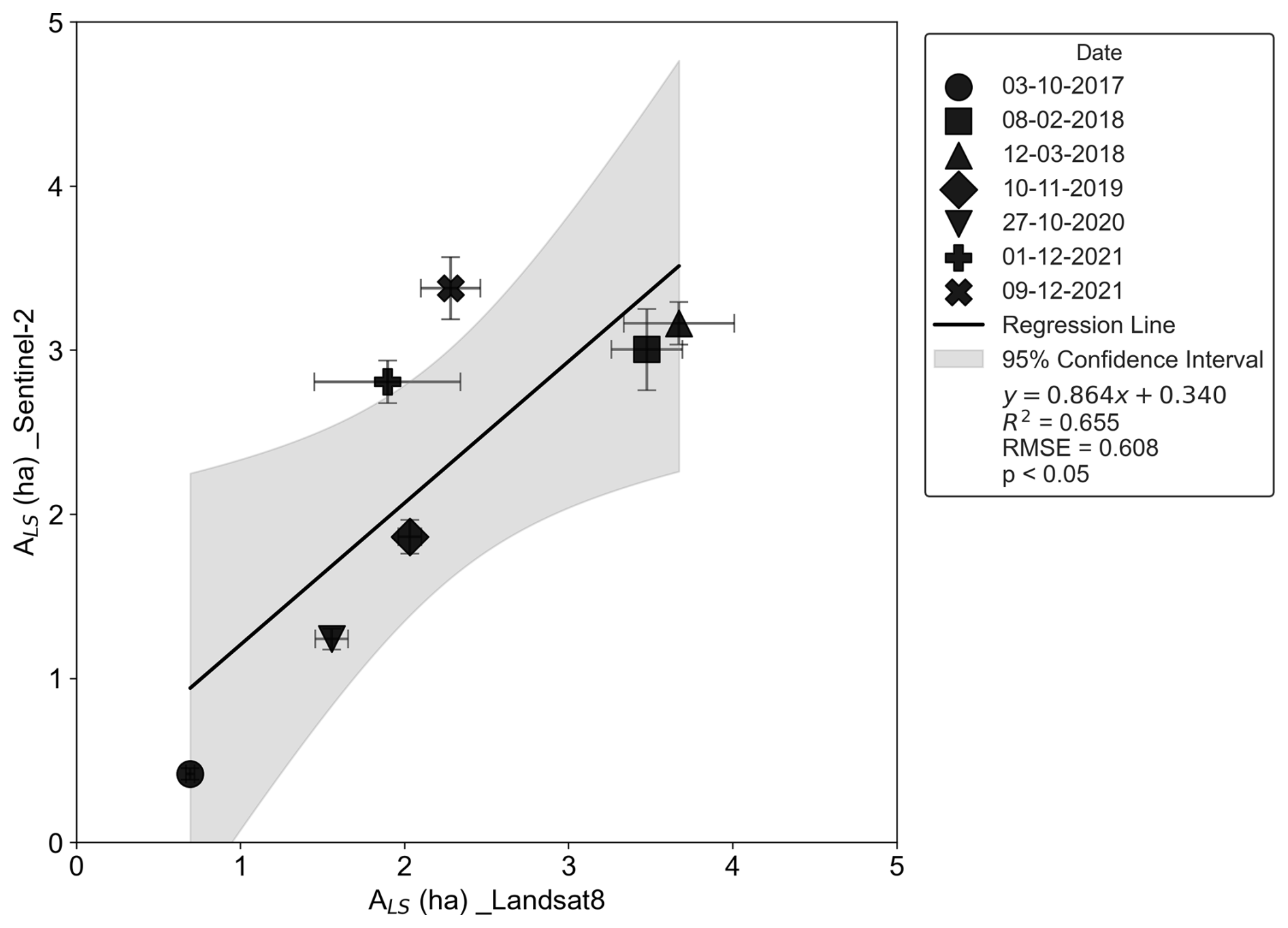
Figure I1Evaluation of resolution-induced errors using Landsat 8 and Sentinel-2 imagery. A significant positive relationship (p<0.05, t-test) indicates that the regression is not a random coincidence.
Annual wind roses for Perapat Tunggal and Selat Baru for 2018 and 2021 are presented in Fig. J1. In Perapat Tunggal, both years exhibit dominant winds from the west and northwest throughout the year, with westerly winds accounting for 16.39 % of the observation. In contrast, in Selat Baru, winds from the east and northeast predominated in both years; in 2018, easterly winds were most frequent at 15.20 %, and in 2021 a maximum wind speed of 20.3 m s−1 was recorded.
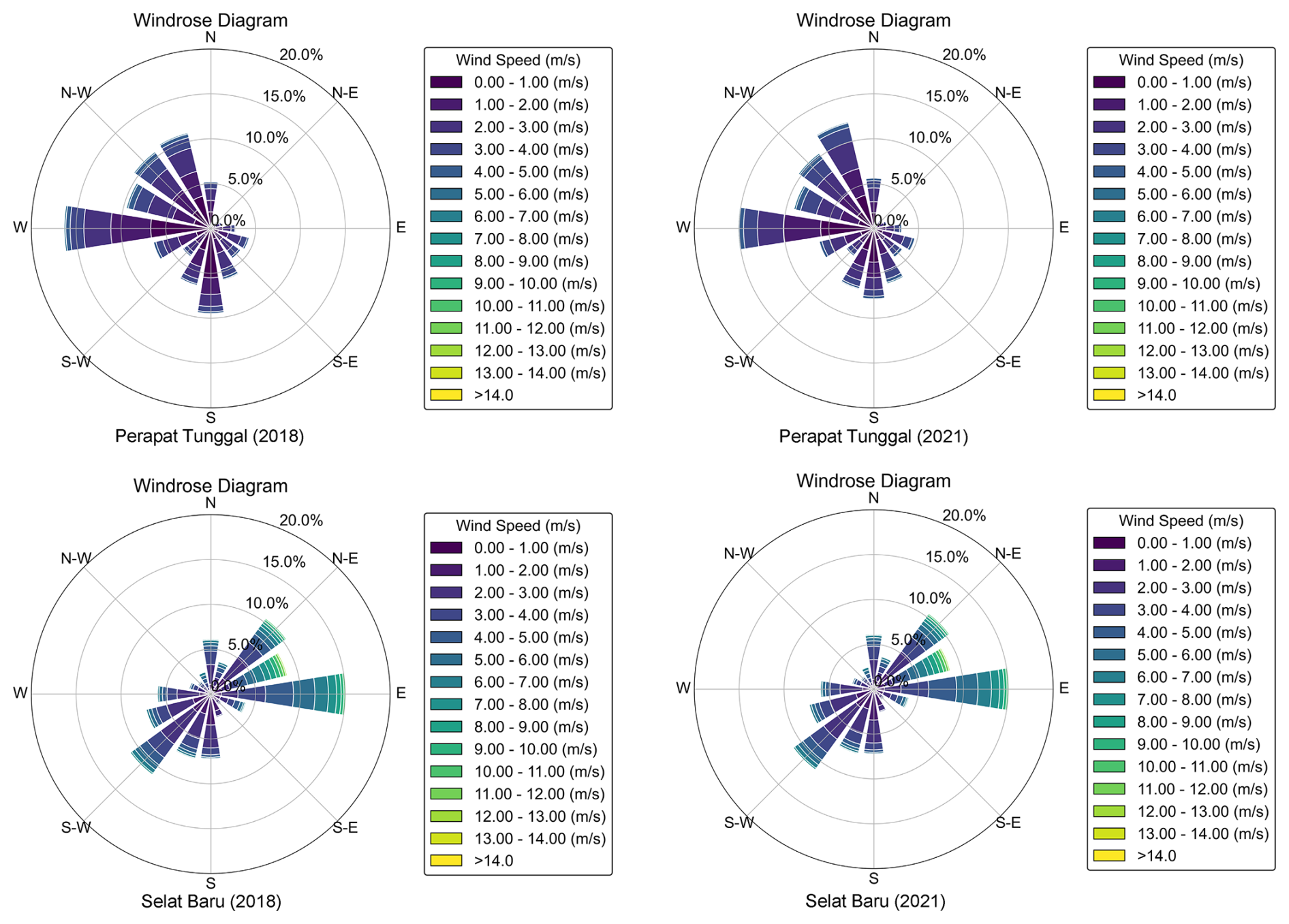
The data for this paper is made available online at https://doi.org/10.5281/zenodo.19159833 (Kagawa et al., 2026).
HK: Writing of the original draft and data analysis. KY: Conceptualisation, Field survey planning, Field survey, and Data analysis. SS: Aerial photogrammetry. MH: Soil sampling. SS and NB: Aerial photogrammetry. AKoyama: Field survey and Soil sampling. AKanno: Field survey. YA, MS: Field survey. All authors contributed to the interpretation of the results and the writing and editing of the final manuscript.
The contact author has declared that none of the authors has any competing interests.
Publisher's note: Copernicus Publications remains neutral with regard to jurisdictional claims made in the text, published maps, institutional affiliations, or any other geographical representation in this paper. The authors bear the ultimate responsibility for providing appropriate place names. Views expressed in the text are those of the authors and do not necessarily reflect the views of the publisher.
This work was supported by JSPS KAKENHI (Grant Numbers 17H01668 and 26303015). The fieldwork was supported by staff and students from the Bengkalis State Polytechnic and the University of Riau. Particulate organic carbon analysis was performed at Saga University with the help of Prof. Yuichi Hayami and Dr. Kenji Yoshino. We also thank Editage (http://www.editage.jp, last access: 26 March 2024) for the English language editing.
This research has been supported by the Japan Society for the Promotion of Science (grant nos. 17H01668 and 26303015).
This paper was edited by Steven Bouillon and Olivier Sulpis and reviewed by two anonymous referees.
Alexander, R. W., Coxon, P., and Thorn, R. H.: A bog flow at Straduff Townland, county Sligo, Proc. R. Ir. Acad. 86B, 107–119, 1986.
Basir, N., Hiraishi, T., and Jauhari, Z.: The Ability of Red Mangrove, Gray Mangrove, and Mangrove Palm to Reduce Erosion Rate at The Northern Coast of Bengkalis Island Indonesia, Proceedings of the 11th International Applied Business and Engineering Conference, ABEC 2023, 21 September 2023, Bengkalis, Riau, Indonesia, https://doi.org/10.4108/eai.21-9-2023.2342878, 2024.
Baum, A., Rixen, T., and Samiaji, J.: Relevance of peat draining rivers in central Sumatra for the riverine input of dissolved organic carbon into the ocean, Estuarine, Coastal and Shelf Science 73, 563–570, https://doi.org/10.1016/j.ecss.2007.02.012, 2007.
Bjerrum, L.: Progressive failure in slopes of overconsolidated plastic clay and clay shales. ASCE Journal of Soil Mechanics and Foundations Division, 93, 3–49, 1967.
Bowes, D. R.: A bog-burst in the Isle of Lewis, Scott. Geogr. J. 76, 21–23, 1960.
Boylan, N., Jennings, R., and Long, M.: Peat slope failure in Ireland, Q. J. Eng. Geol. Hydrogeol., 41, 93–108, https://doi.org/10.1144/1470-9236/06-028, 2008.
Chambers, L. G., Steinmuller, H. E., and Breithaupt, J. L.: Toward a mechanistic understanding of “peat collapse” and its potential contribution to coastal wetland loss, Ecology, 100, https://doi.org/10.1002/ecy.2720, 2019.
Chevallier, D., Glrondot, M., Péron, C., Martin, J., Bonola, M., Chevalier, J., Thoisy, B. D., Kelle, L., Maho, Y. L., Gardel, A., and Anthony, E. J.: Beach erosion aggravates the drastic decline in marine turtle populations in French Guiana, Regional Environmental Change, 23, 116, https://doi.org/10.1007/s10113-023-02105-3, 2023.
Couwenberg, J., Dommain, R., and Joosten, H.: Greenhouse gas fluxes from tropical peatlands in south-east Asia, Global Change Biology, 16, 1715–1732, https://doi.org/10.1111/j.1365-2486.2009.02016.x, 2010.
Dariah, A., Susanti, E., Mulyani, A., and Agus, F.: Faktor penduga simpanan karbon pada tanah gambut [Probe factors (proxy) of carbon stock in peatland], in: Prosiding Seminar Nasional Pengelolaan Lahan Gambut Berkelanjutan (Bogor, 4 May 2012), edited by: Husen, E., Anda, M., Noor, M., Mamat, H. S., Maswar, Fahmi, A., and Sulaeman, Y., Badan Penelitian dan Pengembangan Pertanian, Kementerian Pertanian, Cimanggu (Bogor), 213–221, https://www.scribd.com/document/401524027/Prosiding-Gambut-2012-full-version-pdf (last access: 9 February 2026), 2013.
Dommain, R., Couwenberg, J., and Joosten, H.: Development and carbon sequestration of tropical peat. domes in south-east Asia: links to post-glacial sea-level changes and Holocene climate variability, Quaternary Science Reviews, 30, 999–1010, https://doi.org/10.1016/j.quascirev.2011.01.018, 2011.
Dykes, A. P. and Jennings, P.: Peat slope failures and other mass movements in western Ireland, August 2008, Q. J. Eng. Geol. Hydrogeol., 44, 5–16, https://doi.org/10.1144/1470-9236/09-020, 2011.
Dykes, A. P. and Warburton, J.: Mass movements in peat: A formal classification scheme, Geomorphology 86, 73–93, https://doi.org/10.1016/j.geomorph.2006.08.009, 2007.
Evans, M. and Lindsay, J.: Impact of gully erosion on carbon sequestration in blanket peatlands, Climate Research Clim Res., 45, 31–41, https://doi.org/10.3354/cr00887, 2010.
Evans, M. G. and Warburton, J.: Geomorphology of Upland Peat: Erosion, Form and Landscape Change, Blackwell Publishing, Oxford, 262 pp., 2007.
Furmanczyk, K. and Dudzińska-Nowak, J.: Effects of extreme storms on coastline changes: a southern Baltic example, J. Coast. Res., 56, 1637–1640, 2009.
Galy, V., Peucker-Ehrenbrink, B., and Eglinton, T.: Global carbon export from the terrestrial biosphere controlled by erosion, Nature, 521, 204–207, https://doi.org/10.1038/nature14400, 2015.
Greifswald Mire Centre: Global Peatland Database, https://greifswaldmoor.de/global-peatland-database-en.html (last access: 8 February 2026), 2024.
Hilton, R. G., Galy, V., Gaillardet, J., Dellinger, M., Bryant, C., O'Regan M., Gröcke, D. R., Coxall, H., Bouchez, J., and Calmels, D.: Erosion of organic carbon in the Arctic as a geological carbon dioxide sink, Nature, 524, 84–87, https://doi.org/10.1038/nature14653, 2015.
Hirano, T., Segah, H., Harada, T., Limin, S., June, T., Hirata, R., and Osaki, M.: Carbon dioxide balance of a tropical swamp forest in Kalimantan, Indonesia, Global Change Biology, 13, 412–425, https://doi.org/10.1111/j.1365-2486.2006.01301.x, 2007.
Hirano, T., Segah, H., Kusin, K., Limin, S., Takahashi, H., and Osaki, M.: Effects of disturbances on the carbon balance in tropical peat swamp forests, Global Change Biology, 18, 3410–3422, https://doi.org/10.1111/j.1365-2486.2012.02793.x, 2012.
Hirano, T., Kusin, K., Limin, S., and Osaki, M.: Carbon dioxide emissions through oxidative peat decomposition on burnt tropical peatland, Global Change Biology, 20, 555–565, https://doi.org/10.1111/gcb.12296, 2014.
Hooijer, A., Page, S., Canadell, J. G., Silvius, M., Kwadijk, J., Wösten, H., and Jauhiainen, J.: Current and future CO2 emissions from drained peatlands in Southeast Asia, Biogeosciences, 7, 1505–1514, https://doi.org/10.5194/bg-7-1505-2010, 2010.
Kagawa, H., Yamamoto, K., Haidar, M., Kanno, A., Akamatsu, Y., Suzuki, M., Sutikno, S., Basir, N., and Sekine, M.: Present condition of coastal erosion in the Islands in Riau Province, Indonesia, in: Proceedings of the Civil Engineering Society G (Environment) (Collection of Research Papers on Environmental Engineering), 73, III_213–III_219, https://doi.org/10.2208/jscejer.73.III_213, 2017.
Kagawa, H., Yamamoto, K.. Sutikno, S., Haidar, M., Noerdin, B., Yoshihisa, A., Kanno, A., Suzuki, M., and Koyama, A.: Dataset for: Estimation of particulate organic carbon export to the ocean from lateral degradations of tropical peatland coasts, Zenodo [data set], https://doi.org/10.5281/zenodo.19159833, 2026.
Kleinen, T., Brovkin, V., von Bloh, W., Archer, D., and Munhoven, G.: Holocene carbon cycle dynamics, Geophysical Research Letters, 37, L02705, https://doi.org/10.1029/2009GL041391, 2010.
Koyama, A., Yamamoto, K., Sutikno, S., Basir, N., and Suzuki, M.: Investigation of Peat Landslide in Indonesia Bengkalis Island by Sounding Test, in: Proceedings of 53rd Geotechnical Engineering Research Meeting (Takamatsu City), https://gbank.gsj.jp/ld/resource/geolis/201970507 (last access: 8 February 2026), 2018.
Lantuit, H. and Pollard, W. H.: Fifty years of coastal erosion and retrogressive thaw slump activity on Herschel Island, southern Beaufort Sea, Yukon Territory, Canada, Geomorphology 95, 84–102, https://doi.org/10.1016/j.geomorph.2006.07.040, 2008.
Lantuit, H., Atkinson, D., Overduin, P. P., Grigoriev, M., Rachold, V., Grosse, G., and Hubberten, H. W.: Coastal erosion dynamics on the permafrost-dominated Bykovsky Peninsula, north Siberia, 1951–2006, Polar Research, 30, 7341, https://doi.org/10.3402/polar.v30i0.7341, 2011.
Lehfeldt, R. and Milbradt, P.: Longshore sediment transport modelling in 1 and 2 dimensions, in: advances in Hydro-science and engineering, in: Proceedings of the 4th International Conference on Hydro-Science and Engineering Abstract (Seoul), https://smileconsult.de/web/files/paper.pdf (last access: 25 March 2026), 2000.
Ludwig, W., Probst, J. L., and Kempe, S.: Predicting the oceanic input of organic carbon by continental erosion, Global Biogeochemical Cycles, 10, 23–41, https://doi.org/10.1029/95GB02925, 1996.
Malpica-Piñeros, C., Barthelmes, A., and Joosten, H.: What, when and how? A review of peatland research in Amazonia, Mires and Peat, 31, 03, https://doi.org/10.19189/MaP.2023.OMB.Sc.2115055, 2024.
Mandanici, E. and Bitelli, G.: Preliminary Comparison of Sentinel-2 and Landsat 8 Imagery for a Combined Use, Remote Sens., 8, 1014, https://doi.org/10.3390/rs8121014, 2016.
Matsuo, H., Yamamoto, K., Imai, T., Nakamura, S., Kagawa, H., Sigit, S., Ahmad, M., Muhamad, Y., and Hendra, S.: Flotation of Peat Particles by Dissolved Organic Matter Eluted from the Re-Deposited Tropical Peat in Tropical Peatland Coast. Journal of Water and Environment Technology, 23, 167–178, https://doi.org/10.2965/jwet.24-085, 2025.
McCahon, C. P., Carling, P. A., and Pascoe, D.: Chemical and ecological effects of a Pennine peat-slide, Environ. Pollut., 45, 275–289, https://doi.org/10.1016/0269-7491(87)90102-3, 1987.
Ministry of the Environment: White Paper, Introduction, Section 1, Subsection 2: Global Environment, https://www.env.go.jp/policy/hakusyo/h14/index.html (last access: 9 February 2026), 2002.
Nabilah, D. H., Wibowo, A. A., and Wardan, K. S.: Detection of Peatland Coastline Changes Due to Land Use Change On Bengkalis Island, Riau, Indonesia, in: Proceedings of 5th International Conference of Geography and Disaster Management 2023, https://doi.org/10.1088/1755-1315/1357/1/012042, 2024.
Nicholls, R. J. and Cazenave, A.: Sea-level rise and its impact on coastal zones, Science, 328, 1517–1520, https://doi.org/10.1126/science.1185782, 2010.
Osaki, M. and Tsuji, N.: Tropical peatland ecosystems, Springer Tokyo, 633 pp., 2016.
Page, S. E., Siegert, F., Rieley, J. O., Boehm, H. D. V., Jaya, A., and Limin, S.: The amount of carbon released from peat and forest fires in Indonesia during 1997, Nature, 420, 61–65, https://doi.org/10.1038/nature01131, 2002.
Page, S. E., Rieley, J. O., and Banks, C. J.: Global and regional importance of the tropical peatland carbon pool, Global Change Biology, 17, 798–818, https://doi.org/10.1111/j.1365-2486.2010.02279.x, 2011.
Pawson, R. R., Lord, D. R., Evans, M. G., and Allott, T. E. H.: Fluvial organic carbon flux from an eroding peatland catchment, southern Pennines, UK, Hydrol. Earth Syst. Sci., 12, 625–634, https://doi.org/10.5194/hess-12-625-2008, 2008.
Pawson, R. R., Evans, M. G., and Allott, T. E. H.: Fluvial carbon flux from headwater peatland streams: Significance of particulate carbon flux, Earth Surface Processes and Landforms, 37, 1203–1212, https://doi.org/10.1002/esp.3257, 2012.
Rachold, V., Brown, J., and Solomon, S. (Eds).: Arctic Coastal Dynamics-Report of an International Workshop, Reports on Polar and Marine Research, 413, 103, https://epic.awi.de/id/eprint/26592/1/BerPolarforsch2002413.pdf (last access: 9 February 2026), 2002.
Ribeiro, K., Pacheco, F. S., Ferreira, J. W., de Sousa-Neto, E. R., Hastie, A., Krieger Filho, G. C., Alvalá, P. C., Forti, M. C., and Ometto, J. P.: Tropical peatlands and their contribution to the global carbon cycle and climate change, Global Change Biology, 27, 489–505, https://doi.org/10.1111/gcb.15408, 2021.
Ritung, S., Wahyunto, Nugroho, K., Sukarman, Hikmatullah, Suparto, and Tafakresnanto, C. : Tim Penyusun Peta Lahan Gambut Indonesia Skala 1:250.000 (Indonesian peatland map at the scale 1:250,000), Indonesian Center for Agricultural Land Resources Research and Development, Bogor, Indonesia, https://repository.pertanian.go.id/handle/123456789/5840 (last access: 9 February 2026), 2011.
Rudiyanto, Minasny, B., Satyanto, B. I., Saptomo, S. K., and McBratney, A. B.: Open digital mapping as a cost-effective method for mapping peat thickness and assessing the carbon stock of tropical peatlands, Geoderma, 313, 25–40, https://doi.org/10.1016/j.geoderma.2017.10.018, 2018.
Rydin, H. and Jeglum, J. K.: The Biology of Peatlands 230–233, Oxford Univ. Press, https://doi.org/10.1093/acprof:osobl/9780199602995.001.0001, 2006.
Scharlemann, J. P., Tanner, E. V., Hiederer, R., and Kapos, V.: Global soil carbon: understanding and managing the largest terrestrial carbon pool, Global soil carbon: understanding and managing the largest terrestrial carbon pool, Carbon Management, 5, 81–91, https://doi.org/10.4155/cmt.13.77, 2014.
Sterr, H.: Assessment of vulnerability and adaptation to sea-level rise for the coastal zone of germany, J. Coast. Res., 24, 380–393, https://doi.org/10.2112/07A-0011.1, 2008.
Supardi, Subekty, A. D., and Neuzil, S. G.: General geology and peat resources of Siak Kanan and Bengkalis Island peat deposits, Sumatra, Indonesia, Geological Society of America Special Paper, 286, 45–61, https://doi.org/10.1130/SPE286-p45, 1993.
Tolunay, D., Kowalchuk, G. A., Erkens, G., and Hefting, M. M.: Aerobic and anaerobic decomposition rates in drained peatlands: Impact of botanical composition, Science of the Total Environment, 930, 172639, https://doi.org/10.1016/j.scitotenv.2024.172639, 2024.
Umarhadi. D. A., Widyatmanti, W., Kumar, P., Yunus, A. P., Khedger, K. M., Kharazi, A., and Avtar, R.: Tropical peat subsidence rates are related to decadal LULC changes: Insights from InSAR analysis, Science of the Total Environment, 816, 151561, https://doi.org/10.1016/j.scitotenv.2021.151561, 2022.
US Army Map Service: Bengkalis, Series T503, NA48-9, https://commons.wikimedia.org/wiki/Category:Maps_by_the_United_States_Army_Map_Service_Series_T503 (last access: 8 February 2026), 1955.
Wahyunto, S. , Ritung, S., and Subagjo, H.: Peta Luas Sebaran Lahan Gambut dan Kandungan Karbon di Pulau Sumatera/Maps of Area of Peatland Distribution and Carbon Content in Sumatra: 1990–2002, Wetlands International – Indonesia Programme & Wildlife Habitat Canada (WHC), Bogor, Indonesia TS59, https://repository.wetlands.or.id/index.php?p=show_detail&id=773 (last access 8 February 2026), 2003.
Warburton, J., Holden, J., and Mills, A. J.: Hydrological controls of surficial mass movements in peat, Earth-Science Reviews, 67, 139–156, https://doi.org/10.1016/j.earscirev.2004.03.003, 2004.
Warren, M., Hergoualc'h, K., Kauffman, J. B., Murdiyarso, D., and Kolka, R.: An appraisal of Indonesia's immense peat carbon stock using national peatland maps: Uncertainties and potential losses from conversion, Carbon Balance and Management, 12, 12, https://doi.org/10.1186/s13021-017-0080-2, 2017.
Warren, M. W., Kauffman, J. B., Murdiyarso, D., Anshari, G., Hergoualc'h, K., Kurnianto, S., Purbopuspito, J., Gusmayanti, E., Afifudin, M., Rahajoe, J., Alhamd, L., Limin, S., and Iswandi, A.: A cost-efficient method to assess carbon stocks in tropical peat soil, Biogeosciences, 9, 4477–4485, https://doi.org/10.5194/bg-9-4477-2012, 2012.
Whittle, A. and Gallego-Sala, A. V.: Vulnerability of the peatland carbon sink to sea-level rise, Sci. Rep. 6, 28758, https://doi.org/10.1038/srep28758, 2016.
Wilford, G. E.: A peat landslide in Sarawak, Malaysia, and its significance in relation to washouts in coal seams, Journal of Sedimentary Research, 36, 244–247, https://doi.org/10.1306/74d7146a-2b21-11d7-8648000102c1865d, 1966.
Witze, A.: Why arctic fires are bad news for climate change, unprecedented wildfires released record levels of carbon, partly because they burnt peatlands, Nature News in Focus, 585, https://doi.org/10.1038/d41586-020-02568-y, 2020.
Wong, P. P., Losada, I. J., Gattuso, J.-P., Hinkel, J., Khattabi, A., McInnes, K. L., Saito, Y., and Sallenger, A.: Coastal systems and low-lying areas, Clim. Change, 2014, 361–409, https://doi.org/10.1017/CBO9781107415379.010, 2014.
Xu, J., Morris, P. J., Liu, J., and Holden, J.: PEATMAP: Refining estimates of global peatland distribution based on metaanalysis, University of Leeds, https://doi.org/10.5518/252, 2017.
Yamamoto, K., Watanabe, T., Okuyama, H., Haidar, M., Noerdin, B., Kanno, A., and Sekine, M.: Peat Coast Erosion of the Bengkalis Island and its Effect on the Groundwater Discharge, in: Proceedings of the Civil Engineering Society B2 (Coastal Engineering), 70, I_1466–I_1470, https://doi.org/10.2208/kaigan.70.I_1466, 2014.
Yamamoto, K., Asakuma, T., Kagawa, H., Sutikno, S., Basir, N., and Kanno, A.: Occurrence and disappearance of temporary peat fan by the landslide at the coastal peat coast, in: Proceedings of the Civil Engineering Society B2 (Coastal Engineering) 75, I_1249–I_1254, https://doi.org/10.2208/kaigan.75.I_1249, 2019a.
Yamamoto, K., Basir, N., Sutikno, S., Kanno, A., Kagawa, H., Suzuki, M., Akamatsu, Y., and Koyama, A.: Tropical peat debris storage in the tidal flat in northern part of the Bengkalis island, Indonesia: ICAnCEE 2018, MATEC Web of Conferences 276, 06002, https://doi.org/10.1051/matecconf/201927606002, 2019b.
Yu, Z.: Holocene carbon flux histories of the world's peatlands: global carbon cycle implications, The Holocene, 21, 761–774, https://doi.org/10.1177/0959683610386982, 2011.
Yunker, M. B., Macdonald, R. W., Fowler, B. R., Cretney, W. J., Dallimore, S. R., and Mclaughlin, F. A.: Geochemistry and fluxes of hydrocarbons to the Beaufort Sea shelf: A multivariate comparison of fluvial inputs and coastal erosion of peat using principal components analysis, Geochimica et Cosmochimica Acta, 55, 255–273, https://doi.org/10.1016/0016-7037(91)90416-3, 1991.
- Abstract
- Introduction
- Study area
- Materials and Methods
- Results and discussion
- Conclusions
- Appendix A: The global distribution of peatlands
- Appendix B: Comparison of carbon export studies in Boreal and Tropical peatlands
- Appendix C: Time series of NDVI data viewed and analysed in Sentinel hub EO browser
- Appendix D: Relationship between NDVI and vegetation cover
- Appendix E: Land cover classification using machine learning
- Appendix F: Vegetation removal from DEMNAS data
- Appendix G: Comparison of optical satellite images and UAV-based orthomosaic and estimation methodology of the volume of the land slide-induced exported peat to the ocean
- Appendix H: Error evaluation method for traced coastal erosion areas and landslide-affected areas in GIS software
- Appendix I: Evaluation of resolution-induced errors using Landsat 8 and Sentinel-2 imagery
- Appendix J: Wind rose derived from field observations
- Data availability
- Author contributions
- Competing interests
- Disclaimer
- Acknowledgements
- Financial support
- Review statement
- References