Emerging Climate Signals in Tropical Oxygen Minimum Zones

The ocean is losing oxygen due to anthropogenic climate change. This loss is particularly worrying when it occurs in naturally low-oxygen regions, such as the Oxygen Minimum Zones (OMZs) found at mid-depth in tropical oceans, because the expansion of OMZs reduces habitable space for marine life and threatens oxygen-dependent ecosystems. However, detecting the emergence of climate-driven signals is challenging due to internal variability. Here, we isolate externally forced signals of tropical OMZ volume change and regional deoxygenation, and determine their time of emergence using the IPSL-CM6A-LR Large Ensemble. We apply time of emergence analysis to identify when climate-driven signals become statistically distinguishable from natural variability. Our results show that tropical OMZ edges consistently expand, with emergence occurring in the second half of the 20th century, which is in phase with regional mean deoxygenation in the tropical Pacific and tropical Atlantic. By contrast, we reveal a marked spatial asymmetry in the emergence of OMZ core and hypoxic volumes between the northern and southern parts of tropical OMZs. While OMZ core volumes in the tropical North Pacific and hypoxic volumes in the tropical North Atlantic expand, the tropical South Pacific OMZ core and the tropical South Atlantic hypoxic volume contract. This contraction in the southern hemisphere is due to a sudden increase in ventilation, reflected by a decrease in the age since surface contact at the start of the 21st century. Uncertainties in emergence timing range from 20 to 30 years across ensemble members, and increase substantially in regions influenced by abrupt changes in OMZ ventilation. By linking the emergence of regional deoxygenation to that of OMZ volume changes, climate-driven expansions of tropical OMZ volumes appear to be beginning to emerge, with distinct dynamics between northern and southern tropical oceans.

1 Introduction

The global ocean is losing oxygen as a consequence of climate warming, with historical observations indicating a ∼2 % global decline in oxygen concentrations over the past 50 years (Keeling et al., 2010; Schmidtko et al., 2017; Ito et al., 2017). Ocean deoxygenation poses a direct threat to aerobic organisms and marine ecosystems (Stramma et al., 2012; Vaquer-Sunyer and Duarte, 2008). Although the distribution of dissolved oxygen is highly heterogeneous in the ocean, oxygen declines have been recorded in both well-oxygenated regions and in areas where concentrations are already critically low, the latter known as Oxygen Minimum Zones (OMZ) (Schmidtko et al., 2017; Ito et al., 2017). Permanent open-ocean OMZs are typically located in poorly ventilated regions of the ocean and beneath zones of high biological productivity, where oxygen consumption is elevated (Wyrtki, 1962; Luyten et al., 1983; Paulmier and Ruiz-Pino, 2009). Consequently, OMZs are found mainly at intermediate depths (∼100 to 1000 m deep) in tropical regions. The largest OMZ is located in the tropical Pacific Ocean, with additional major OMZs in the tropical Atlantic and the North Indian Ocean.

OMZs are regions of the ocean in which dissolved oxygen concentrations fall below the hypoxic threshold, posing a threat to oxygen-dependent marine life (Stramma et al., 2008). In their core, oxygen levels can drop even further, sometimes below anoxic thresholds (Stramma et al., 2008). Although deoxygenation rates tend to be lower in these already hypoxic areas compared to better ventilated regions, ongoing oxygen loss can lead to expansion of OMZs (Stramma et al., 2008; Deutsch et al., 2014; Ito et al., 2017; Levin, 2018). This potential increase in the volume of OMZ is a critical concern, as it could reduce the habitable space available to marine ecosystems (Stramma et al., 2012; Levin, 2018). Therefore, it is essential to assess future levels of deoxygenation along with changes in OMZ volume, as both factors combine to determine the extent and intensity of low-oxygen habitats. However, it remains challenging to track long-term volume changes directly from observations due to sparse spatial coverage and limited time series; this makes Earth System Models essential for identifying large-scale patterns and anticipating future changes.

Although there is strong evidence that ocean deoxygenation will continue to intensify in response to climate change, projections of future OMZ volume changes remain highly uncertain (Resplandy, 2018; Bahl et al., 2019; Kwiatkowski et al., 2020; Lévy et al., 2022). OMZ volume changes are governed by the balance between water mass ventilation and biological oxygen consumption (Resplandy, 2018), and this balance is not consistently represented in coarse-resolution ESMs (Lévy et al., 2022). A key source of uncertainty lies in the parameterization of mixing, which directly affects oxygen supply through ventilation and indirectly impacts oxygen consumption through biological processes (Duteil and Oschlies, 2011; Bahl et al., 2019). For these reasons, previous studies based on Earth System Models (ESM) from Phase 5 of the Coupled Model Intercomparison Project (CMIP5, Taylor et al., 2012) failed to reach consensus on OMZ expansion or contraction, particularly in the tropics (Bopp et al., 2013; Cabré et al., 2015).

Shifting the analysis of OMZ evolution from a geographic-space to an oxygen-space framework helped reconcile apparent discrepancies in projections across models (Ditkovsky and Resplandy, 2025). Within this oxygen framework, OMZ projections from the Coupled Model Intercomparison Project Phase 6 (CMIP6, Eyring et al., 2016) could be coherently categorized into three distinct regimes: the OMZ core, projected to shrink; hypoxic waters, which represent a transitional regime with uncertain future trends; and low-oxygen waters, projected to expand due to reduced ventilation (Busecke et al., 2022; Ditkovsky et al., 2023). This categorisation helped reduce the spread among CMIP6 model projections.

Despite statistically significant trends in OMZ volumes identified using CMIP6 models (Busecke et al., 2022; Ditkovsky et al., 2023), attributing these trends to externally forced climate change remains challenging due to strong internal variability (Ito and Deutsch, 2010; Poupon et al., 2023). This internal variability is a natural and intrinsic dynamic of the coupled model, arising from non linear natural dynamical processes and interactions among climate system components (Lorenz, 1963; Hasselmann, 1976). For a forced signal to be detectable, the externally forced trend must persistently emerge above internal variability, which is considered as noise (Hasselmann, 1993; Santer et al., 1994). This notion of emergence is crucial, as it marks the point at which climate-driven changes can be confidently separated from internal variability and thus when oxygen concentrations are forced beyond natural conditions experienced by marine ecosystems.

However, when performing a single simulation using an Earth System Model, externally-forced (natural and anthropogenic) changes of deoxygenation and OMZ volumes are intertwined with internal variability (Deser et al., 2012). Although the climate-driven signal is often approximated by a linear trend, single simulation analysis fails to capture the non-linearity of external forcing. Consequently, it inaccurately represents the amplitude of long-term changes, while also misrepresenting the amplitude and phase of the estimated internal variability (Mann, 2008; Frankcombe et al., 2015).

To overcome these limitations, Large Ensembles, consisting of multiple simulations, are essential to isolate forced climate signals from internal variability. With a sufficiently large number of simulations, the spread arises purely from internal variability, and the climate-driven signal can be isolated through ensemble averaging (Deser et al., 2012).

In this study, we pursue two main objectives: identify climate-driven changes in ocean deoxygenation and OMZ volumes, and assess the time at which these signals emerge from internal variability. In doing so, we aim to bridge the gap between what can currently be observed and what might be detectable in the future, by using models to explore when that change becomes or has become distinguishable from natural variability.

We conduct a regional analysis across five key OMZ regions to assess co-evolution of deoxygenation and OMZ volumes under ocean warming: the tropical North Pacific, tropical South Pacific, tropical North Atlantic, tropical South Atlantic, and North Indian Ocean. We track the evolution of dissolved oxygen and OMZ volumes using the oxygen-space framework developed by Ditkovsky and Resplandy (2025). Following the regimes identified by Ditkovsky et al. (2023), we distinguish three OMZ volume classes: OMZ core volumes ([O₂]<20 µmol kg⁻¹), where nitrous oxide is produced (Ji et al., 2015; Bianchi et al., 2018); hypoxic volumes ([O₂]<60 µmol kg⁻¹), which are harmful to many marine organisms (Miller et al., 2002; Vaquer-Sunyer and Duarte, 2008); and low-oxygen volumes ([O₂]<120 µmol kg⁻¹), which influence the distribution of marine ecosystems (Bertrand et al., 2011). To isolate the externally forced climate signal, we leverage the IPSL-CM6A-LR Large Ensemble (Bonnet et al., 2021), which consists of 32 ensemble members. The IPSL-CM6A-LR Large Ensemble has already proven effective in extracting the anthropogenic component of ocean warming (Silvy et al., 2022). We apply the concept of time of emergence, which quantifies when the forced climate signal becomes distinguishable from internal variability (Hawkins and Sutton, 2012). Previous studies have used this method to detect the emergence of deoxygenation at the global scale (Long et al., 2016; Hameau et al., 2019), in regional basins (Gong et al., 2021), and at various depths (Gong et al., 2021). While these studies focused on oxygen concentrations, we extend the method to OMZ volume metrics, providing a complementary perspective on the detectability of low-oxygen changes under climate forcing.

2 Materials and methods

2.1 Model and simulations

2.1.1 IPSL-CM6A-LR description

The model used for this study is the IPSL-CM6A-LR (Boucher et al., 2020), an Earth System Model (ESM) developed by the Institut Pierre Simon Laplace (IPSL). The model was one of the models contributing to the sixth phase of the Coupled Model Intercomparaison Project (CMIP6, Eyring et al., 2016). It couples three modules: the LMDZ atmospheric model version 6A-LR (Hourdin et al., 2020), the ORCHIDEE land surface model version 2.0 (Krinner et al., 2005) and the NEMO ocean model version 3.6 (Madec et al., 2017). The ocean module of the model includes three major components: the ocean physics NEMO-OPA (Madec et al., 2017), the sea ice dynamics and thermodynamics NEMO-LIM3 (Rousset et al., 2015; Vancoppenolle et al., 2009), and the ocean biogeochemistry NEMO-PISCES (Aumont et al., 2015).

The atmospheric module uses a 2.5° × 1.3° horizontal resolution and 79 vertical levels. The ocean module uses the eORCA1 configuration which is a tripolar grid with a 1° nominal resolution and a refinement to $\mathrm{1}/\mathrm{3}$° in the equatorial region. The eORCA1 grid has 75 vertical levels.

The O₂ concentrations are used in the model in mmol m⁻³ and are subsequently converted to µmol kg⁻¹ using a constant reference density of ρ₀=1025 kg m⁻³.

2.1.2 IPSL-CM6A-LR Large Ensemble

This study uses the Large Ensemble of the IPSL-CM6A-LR model. The Large Ensemble consists of a piControl simulation and 32 historical-EXT experiences (Bonnet et al., 2021). The piControl run is a 2000 years control simulation using pre-industrial climate forcing. The historical-EXT simulations are initialised from different years of the piControl and run for 210 years (Fig. 1a). Initialisation conditions of historical-EXT ensemble are picked out from the piControl experiment every 20 years, in order to sample the phases of the bicentennial variability present in global mean surface air temperature of the model (Bonnet et al., 2021). Thus, initialisations of historical-EXT occur between the 20th and the 830th year of piControl simulation time, collectively sampling three cycles of this low-frequency variability. All of the historical-EXT are run under the CMIP6 historical procedure during 164 years (1850–2014) and then extended from 2015 to 2060 using radiative forcing of the SSP2-4.5 scenario, except for the ozone field which has been kept constant to its 2014 climatology (O’Neill et al., 2016; Bonnet et al., 2021). Due to file corruption, member r2i1p1f1 and member r16i1p1f1 were rejected and only 30 members were considered.

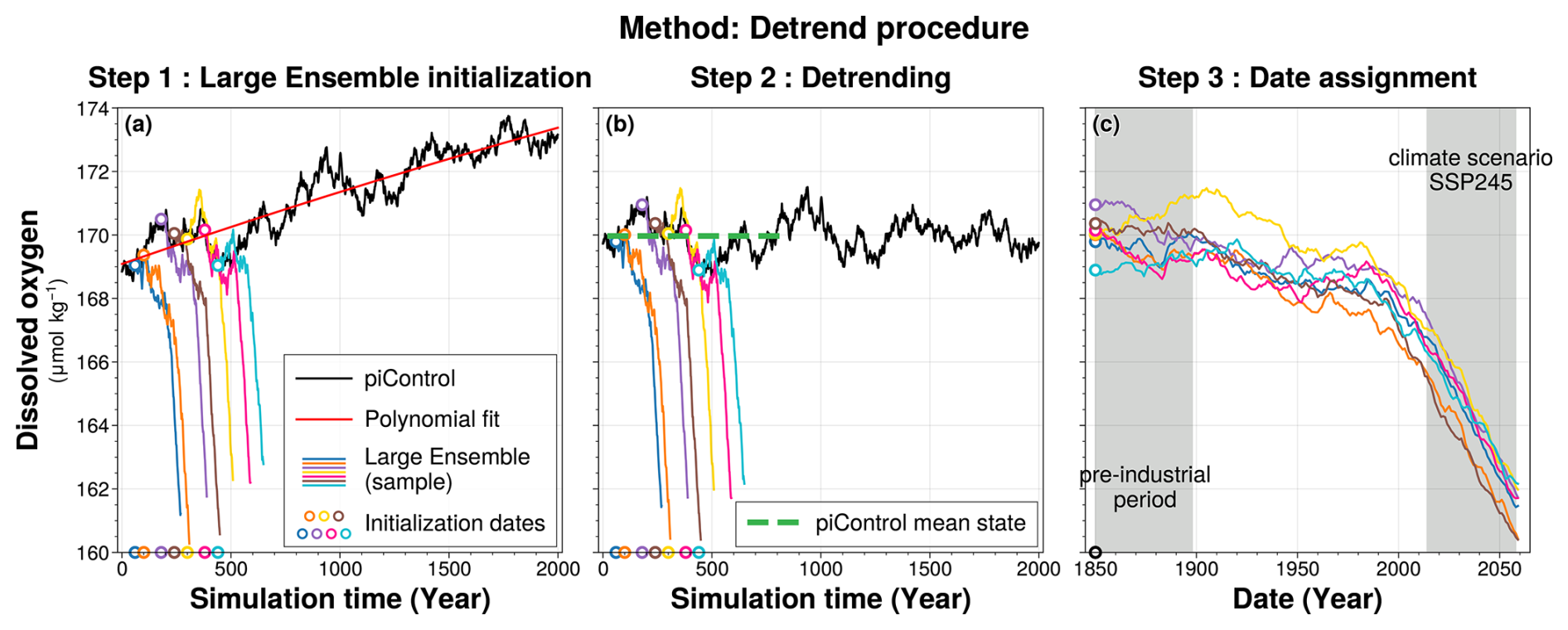
Figure 1 Detrend procedure for global ocean mean of dissolved oxygen concentration between 100–1000 m depth. Time series from the piControl simulation are shown in black in both panels (a) and (b). In all three panels, coloured lines represent a subset of 7 ensemble members (out of the 30) from the historical-EXT simulation of the IPSL-CM6A-LR model: members 1, 4, 6, 9, 11, 17, and 22. The starting points of each member are marked by coloured rings, with the ring colours corresponding to the respective lines. Panel (a) shows the raw data, with the drift from the piControl simulation in red. Panel (b) shows the detrended data, with the green line indicating the piControl mean state over the simulation period 20–830. Panel (c) shows the historical-EXT ensemble members shifted to the simulation forcing years, 1850–2059.

Each member of the IPSL-CM6A-LR ensemble contains both the climate-driven signal and some internal variability of the climate system. Large ensembles are useful tools to isolate these two components. By averaging across multiple members, defining the Large Ensemble mean, the forced signal is extracted from the internal variability of the climate system. Internal variability can thus be estimated by the spread among members, measured by its standard deviation (Deser et al., 2012).

2.1.3 Model drift correction

The piControl simulation in IPSL-CM6A-LR has a quasi-linear cooling drift in global mean ocean temperature, originating from a mean net surface heat loss (Mignot et al., 2021). This drift propagates into the historical simulations and onto the oxygen concentration evolution. To correct for this drift, we followed the methodology of Silvy et al. (2022). While the method is applied at each grid point, Fig. 1 illustrates its implementation using the global mean oxygen concentration over the 100–1000 m depth range for clarity. We fitted a second order polynomial to the 2000 year piControl annual means (Fig. 1a). Using the full piControl period ensures that the drift is isolated, preventing the capture of low-frequency internal variability (Gupta et al., 2013). We then subtracted the corresponding 210 year segment of this polynomial fit from each ensemble member, aligning with its respective piControl period, and subsequently added the same mean state back to each member (Fig. 1b). This mean state is defined as the mean of the piControl calculated over the period when the historical-extended simulations were performed, spanning simulation years 20 to 830 of piControl simulation. By adding this mean state, we preserve absolute oxygen concentrations rather than anomalies.

After this correction, the spread across all 30 members reflects only differences in phasing of internal variability, as their mean states are no longer shifted by their initialisation in the drifting piControl. Consequently, the IPSL-CM6A-LR Large Ensemble consists of 30 historical-EXT simulations, all forced by the same historical and SSP2-4.5 climate scenario, with variations arising purely from differences in the phasing of internal variability dictated by their initial conditions (Fig. 1c).

2.2 Model evaluation

Here, we evaluate the representation of dissolved oxygen content and deoxygenation trends in the IPSL-CM6A-LR Large Ensemble simulations (Figs. 2 and 3).

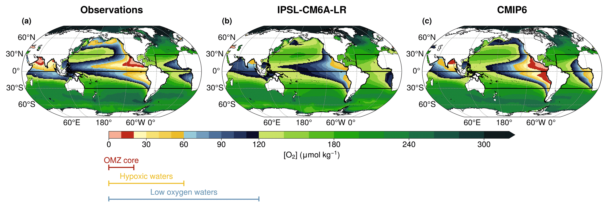
Figure 2 Vertical mean dissolved oxygen concentration between 100–1000 m for the present-day period (1970–2014) climatology, using (a) the World Ocean Atlas 2018 dataset, (b) the IPSL-CM6A-LR Large Ensemble mean, and (c) the CMIP6 multi-model ensemble mean. The colourbar indicates oxygen concentration boundaries: (red) OMZ core below 20 µmol kg⁻¹, (yellow) hypoxic waters below 60 µmol kg⁻¹ and (blue) low-oxygen waters below 120 µmol kg⁻¹. In all panels, the black boxes represent the five domains considered in this study.

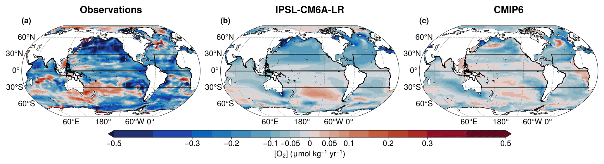
Figure 3 Vertical mean dissolved oxygen trends between 100–1000 m for the present-day period (1970–2014), using (a) the Cheng and Gouretski (2023) dataset, (b) the IPSL-CM6A-LR Large Ensemble mean, and (c) the CMIP6 multi-model ensemble mean. In all panels, black boxes represent the five domains considered in this study.

2.2.1 Datasets

We use oxygen data from the World Ocean Atlas 2018 (WOA18, García et al., 2018) to evaluate the oxygen content in the IPSL-CM6A-LR Large Ensemble simulations. WOA18 provides an objectively analysed climatology of in situ dissolved oxygen measurements, offering a robust reference for large-scale oceanic oxygen distributions.

To evaluate present-day oxygen trends (1970–2014) in the IPSL-CM6A-LR Large Ensemble, we use the Institute of Atmospheric Physics (IAP) dataset from the Chinese Academy of Sciences (Cheng and Gouretski, 2023). This time-dependent dataset integrates observations from CTD, Argo floats, and bottle samples. To correct biases in Argo measurements, Cheng and Gouretski (2023) applied quality control procedures from Gouretski et al. (2024) and interpolated the data onto a 1° grid using the method described in Cheng and Zhu (2016).

Additionally, we evaluate the performance of the IPSL-CM6A-LR model by comparing it against outputs from 10 other Earth System Models (ESMs) that participated in the CMIP6 project (Eyring et al., 2016). The selection of the models was based on the availability of dissolved oxygen variable necessary to evaluate IPSL-CM6A-LR model. The models are ACCESS-ESM1-5 (Ziehn et al., 2020), CanESM5 (Swart et al., 2019), CNRM-ESM2-1 (Séférian et al., 2019), GFDL-CM4 (Held et al., 2019), GFDL-ESM4 (Dunne et al., 2020; Stock et al., 2020), MIROC-ES2L (Hajima et al., 2020), MPI-ESM1-2-HR (Müller et al., 2018; Mauritsen et al., 2019), MRI-ESM2-0 (Yukimoto et al., 2019), NorESM2-LM (Tjiputra et al., 2020), and UKESM1-0-LL (Sellar et al., 2019). All models are assessed over the present-day period (1970–2014) following the CMIP6 historical protocol and over climate change scenario period (2015–2059) following the SSP2-4.5 scenario protocol (O’Neill et al., 2016). The analysis focuses on the 100–1000 m depth range, and results from individual models are averaged to compute the CMIP6 multi-model mean.

2.2.2 Model evaluation of oxygen

In this section, we evaluate the present-day (1970–2014) dissolved oxygen climatology in IPSL-CM6A-LR against observations from WOA18 and other CMIP6 models. Specifically, we compare the present-day climatologies of WOA18 and the CMIP6 multi-model mean with the IPSL-CM6A-LR Large Ensemble mean climatology over the same period (Fig. 2). All climatologies are computed at fixed depths, between 100 and 1000 m.

We focus on the representation of three key oxygen concentration thresholds, which are critical for climate and marine ecosystems (Fig. 2): oxygen concentrations below 20 µmol kg⁻¹, corresponding to the core of the OMZs; oxygen concentrations below 60 µmol kg⁻¹, defining hypoxic waters; oxygen concentrations below 120 µmol kg⁻¹, representing low-oxygen waters.

The IPSL-CM6A-LR model shows an oxygen surplus (Fig. 2b), resulting in a misrepresentation of oxygen concentrations (Aumont et al., 2015). While the model provides a better representation of low-oxygen waters compared to hypoxic waters and OMZ cores, it still underestimates hypoxic waters and fails to capture the OMZ cores (Fig. 2b). The IPSL-CM6A-LR model fails to capture hypoxic waters in the subarctic Pacific (Fig. 2a and b). In the tropical North Pacific and North Indian Ocean, observations reveal well-defined OMZ core waters, which are absent in the simulation (Fig. 2a and b). In the North Indian Ocean, the IPSL climatology shows an oxygen minimum in the Bay of Bengal (Fig. 2b) but fails to represent hypoxic waters and OMZ core in the Arabian Sea, both of which are present in observations (Fig. 2a and b). As a result, in the North Indian Ocean, in the IPSL model the volume of hypoxic water is only 10 % of that in the observational data product. In the tropical Pacific, hypoxic waters are also underestimated, representing 24 % of the observed volume in the tropical North Pacific and 42 % in the tropical South Pacific (Fig. 2a and b). However, the IPSL model successfully captures the north-south structure of the tropical Pacific hypoxic waters (Fig. 2a and b). A key feature of this structure is the higher dissolved oxygen concentrations along the Equator, compared to lower concentrations on either side, leading to the equatorial separation of the OMZ core (Busecke et al., 2022). IPSL model fails to reproduce the low-oxygen waters structure in the tropical Atlantic basin, where only the tropical South Atlantic low-oxygen waters are simulated (Fig. 2b). Across all regions, the IPSL simulations systematically overestimate oxygen concentrations compared to observations (Figs. 2a and A1).

The misrepresentation of dissolved oxygen is not unique to IPSL-CM6A-LR model. It is also present in the CMIP6 multi-model climatology (Fig. 2c). Like IPSL, CMIP6 models fail to capture OMZ core waters in the North Indian Ocean, with an oxygen minimum in the Bay of Bengal rather than in the Arabian Sea. However, in the tropical North Pacific and tropical North Atlantic, CMIP6 models better represent low-oxygen waters (Fig. 2c). OMZ core waters are present in the tropical North Pacific in the CMIP6 mean. In the tropical South Pacific and tropical South Atlantic, CMIP6 models underestimate dissolved oxygen. Overall, the IPSL-CM6A-LR climatology simulates higher oxygen levels than the CMIP6 multi-model mean (Fig. A1).

2.2.3 Model evaluation of deoxygenation

In this section, we evaluate trends in dissolved oxygen in the IPSL-CM6A-LR Large Ensemble mean by comparing them with observations from the Institute of Atmospheric Physics dataset (Cheng and Gouretski, 2023) and other CMIP6 models (Fig. 3). These trends are computed over a fixed depth range between 100 and 1000 m using ordinary least-squares linear regression for all datasets (von Storch and Zwiers, 1999). The uncertainties of the trends are estimated with an 90 % confidence interval, computed based on von Storch and Zwiers (1999): $[a+t_{\mathrm{5}\mathit{\%}}{s}_a;a+t_{\mathrm{95}\mathit{\%}}{s}_a]$ where a is the estimated trend, t_5 % and t_95 % are the 5 % and 95 % percentiles for a Student law taking into account the degrees of freedom and s_a is the standard error of the estimated trend.

Firstly, we examine present-day trends over the period 1970–2014. All members of the IPSL Large Ensemble exhibit a global decline in oceanic dissolved oxygen. The ensemble mean shows a decrease of 1.2 % in global mean oxygen concentration, which is greater than the decline of 0.95 % showed by the CMIP6 multi-model mean. However, both IPSL Large Ensemble and CMIP6 multi-model underestimate the observed oxygen decline. The IAP dataset shows a reduction of 2.8 % over the present day period. This underestimation is also reflected in the linear trends of deoxygenation. The IPSL Large Ensemble simulates a global mean deoxygenation rate of 0.053 ± 0.023 $\mathrm{\mu }\mathrm{mol}{\mathrm{kg}}^{-\mathrm{1}}{\mathrm{yr}}^{-\mathrm{1}}$, exceeding the CMIP6 multi-model deoxygenation mean rate of 0.036 ± 0.022 $\mathrm{\mu }\mathrm{mol}{\mathrm{kg}}^{-\mathrm{1}}{\mathrm{yr}}^{-\mathrm{1}}$, yet still considerably lower than the observed deoxygenation trend of 0.13 ± 0.097 $\mathrm{\mu }\mathrm{mol}{\mathrm{kg}}^{-\mathrm{1}}{\mathrm{yr}}^{-\mathrm{1}}$ from the IAP dataset.

The IPSL-CM6A-LR Large Ensemble mean and CMIP6 multi-model mean show a spatial distribution of present-day deoxygenation that is consistent with IAP observation dataset (Fig. 3). Both IPSL Large Ensemble and CMIP6 multi-model show stronger deoxygenation rates at high latitudes, in agreement with the IAP dataset (Fig. 3). However, regional trends in the models are weaker than those observed (Fig. 3). Observations indicate oxygenation in the Southern Hemisphere, particularly in the South Pacific and South Indian Oceans (Fig. 3a). The IPSL Large Ensemble captures this oxygenation trend in both regions (Fig. 3b). The tropical Pacific shows deoxygenation in both observations and IPSL simulations (Fig. 3a and b). In the Atlantic basin, IPSL simulations show widespread deoxygenation but fails to reproduce regional oxygenation trends. Both the IAP dataset and the CMIP6 multi-model mean capture oxygenation in the North Atlantic and the Benguela upwelling system (Fig. 3). Similarly, in the North Indian Ocean, the IPSL simulations fail to reproduce the observed spatial pattern of oxygenation and deoxygenation. Both the IAP dataset and the CMIP6 multi-model mean indicate oxygenation in the central basin, surrounded by deoxygenation to the north and south (Fig. 3).

Then, we assess future trends under SSP2-4.5 climate scenario forcing over the period 2015–2059. The IPSL-CM6A-LR Large Ensemble mean shows a stronger deoxygenation trend than during the present-day period, with a global mean oxygen decline of 0.11 ± 0.030 $\mathrm{\mu }\mathrm{mol}{\mathrm{kg}}^{-\mathrm{1}}{\mathrm{yr}}^{-\mathrm{1}}$. All historical-EXT members of the IPSL Large Ensemble show deoxygenation trends under the SSP2-4.5 scenario, consistent with the ensemble mean (Fig. 1c). The IPSL-simulated deoxygenation rate is higher than CMIP6 multi-model projections, as the CMIP6 multi-model mean shows a global oxygen decline of 0.054 ± 0.0041 $\mathrm{\mu }\mathrm{mol}{\mathrm{kg}}^{-\mathrm{1}}{\mathrm{yr}}^{-\mathrm{1}}$.

2.3 Deoxygenation and OMZ metrics

To investigate the response of OMZs to ongoing ocean deoxygenation, both phenomena need to be tracked within consistent spatial domains. This approach enables a direct comparison between OMZ dynamics and its corresponding regional deoxygenation trends. We define five fixed regional boxes corresponding to the major tropical OMZs (Figs. 2 and 5): tropical North Pacific (0° S–30° N / 120–295° E), tropical South Pacific (30° S–0° N / 120–295° E), tropical North Atlantic (0° S–30° N / 60° W–20° E), tropical South Atlantic (30° S–0° N / 60° W–20° E) and North Indian (0° S–30° N / 35–120° E). As the IPSL-CM6A-LR model fails to represent oxygen minimum in the subarctic Pacific, this OMZ region has not been included in the analysis. We also restrict our analysis to the 100–1000 m depth range, where dissolved oxygen concentrations are at their lowest.

Ocean deoxygenation is quantified by tracking temporal trends in spatially averaged, both vertical and horizontal, dissolved oxygen concentrations within each box.

OMZ metrics are commonly defined as the ocean volume with oxygen concentration below a given threshold (Busecke et al., 2022), hereafter referred to as the fixed-threshold approach. However, as demonstrated in the model evaluation, the IPSL-CM6A-LR Large Ensemble does not accurately reproduce the observed locations and extent of OMZ core waters, hypoxic waters and low-oxygen waters, limiting the relevance of analysing OMZ changes in the geographic space (Fig. 2). To overcome this limitation, we adopt the fixed volume-percentile approach, based on the “oxygen water mass framework” developed by Ditkovsky and Resplandy (2025).

In this framework, water masses are characterised by the oxygen-percentile relation ${\mathrm{O}}_{\mathrm{2}}^{*}(p,t)$ (Ditkovsky and Resplandy, 2025). The oxygen-percentile p represents the proportion of ocean volume with oxygen concentrations below ${\mathrm{O}}_{\mathrm{2}}^{*}$ at time t, computed as (Sohail et al., 2021; Ditkovsky and Resplandy, 2025),

$$\begin{array}{}\text{(1)}& p({\mathrm{O}}_{\mathrm{2}}^{*},t)=\mathrm{100}\cdot \mathcal{V}({\mathrm{O}}_{\mathrm{2}}^{*},t)/{\mathcal{V}}_{\mathrm{T}}\end{array}$$

with 𝒱_T being the total volume considered and $\mathcal{V}({\mathrm{O}}_{\mathrm{2}}^{*},t)$ is the volume of water with ${\mathrm{O}}_{\mathrm{2}}<{\mathrm{O}}_{\mathrm{2}}^{*}$.

The oxygen-percentile relations are computed using both the WOA18 climatology and the IPSL-CM6A-LR mean averaged over the present day period (1970–2014) (Fig. 4). It is computed within each of the five OMZ regions (Fig. 4). The IPSL model captures the overall shape of the oxygen–percentile relation observed in the WOA18 dataset (Fig. 4), although it generally overestimates oxygen concentrations. Consequently, for a given percentile, the model corresponds to a higher oxygen threshold, except in the tropical South Pacific and tropical South Atlantic. In the former, a positive bias is observed below the 47th percentile; in the latter, a positive bias appears below the 29th percentile and a negative bias above it (Fig. 4). These biases are consistent with the model oxygen content surplus and spatial mismatches previously described.

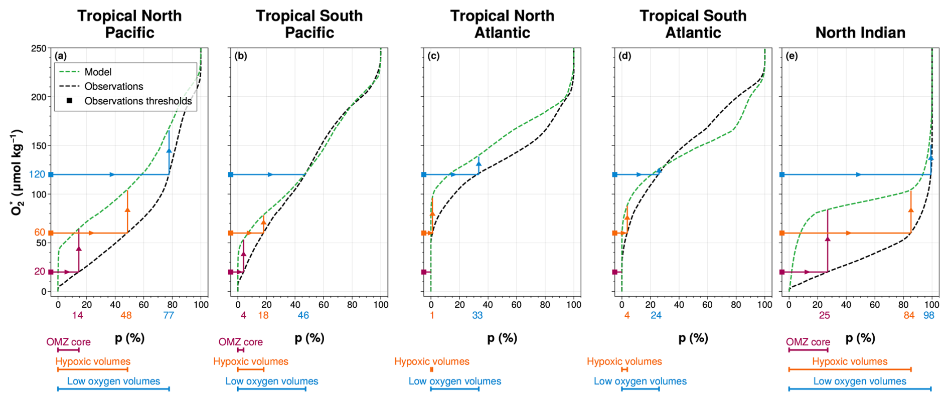
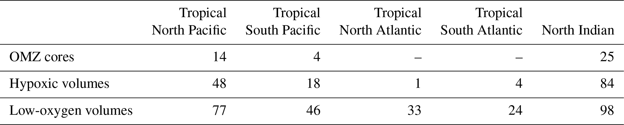
Figure 4 OMZ volume definition in IPSL-CM6A-LR simulations. For (a) the tropical North Pacific, (b) the tropical South Pacific, (c) the tropical North Atlantic, (d) the tropical South Atlantic and (e) the North Indian ocean, the volume percentile p is computed as a function of O₂ threshold using (black dashed lines) the World Ocean Atlas database and (green dashed lines) the IPSL-CM6A-LR Large Ensemble mean. The three thresholds ((purple) 20 µmol kg⁻¹, (orange) 60 µmol kg⁻¹ and (blue) 120 µmol kg⁻¹) define (coloured bands) the three volume percentiles of interest for each OMZ spatial box in WOA: (purple) OMZ core, (orange) hypoxic volumes and (blue) low-oxygen volumes (Table 1). These percentiles are then used to compute the corresponding OMZ volumes in the IPSL-CM6A-LR simulations (arrowed lines).

To account for these systematic biases, we define OMZ volumes using percentile thresholds derived from WOA18. In each region, we identify the percentile corresponding to three key oxygen thresholds in the WOA18 climatology: 20 µmol kg⁻¹ for OMZ core waters; 60 µmol kg⁻¹ for hypoxic waters; and 120 µmol kg⁻¹ for low-oxygen waters. In the Atlantic basin, oxygen concentrations in observations do not fall below 20 µmol kg⁻¹; therefore, the OMZ core is not defined in the tropical North and South Atlantic (Fig. 4). The percentiles associated with these thresholds are then applied to the IPSL oxygen–percentile curves, allowing consistent identification of the three OMZ volume categories in both observations and simulations (Fig. 4, Table 1). This method enables us to track the evolution of OMZ volumes and their oxygen content over time while taking into account the model’s oxygen biases.

Table 1 Volume percentile of interest derived from World Ocean Atlas 2018 and applied to the IPSL-CM6A-LR Large Ensemble mean for each OMZ spatial box. The volume percentile is computed as fraction (%) of the total volume of respective OMZ spatial box.

We further analyse the spatial distribution of OMZ volumes (Fig. 5). Across all OMZ volume classes, the thickest areas of OMZ volumes in the IPSL simulations align with those observed in WOA18. However, in observations, OMZ thickness decreases sharply at their boundaries with sharp oxygen concentration gradient, whereas in the IPSL Large Ensemble mean, the transition is more gradual, resulting in more extensive OMZ volumes (Fig. 5). Additionally, the North Indian OMZ core and hypoxic volume in the model are predominantly located in the Bay of Bengal, whereas observations indicate a signal both in the Arabian Sea and the Bay of Bengal (Fig. 5).

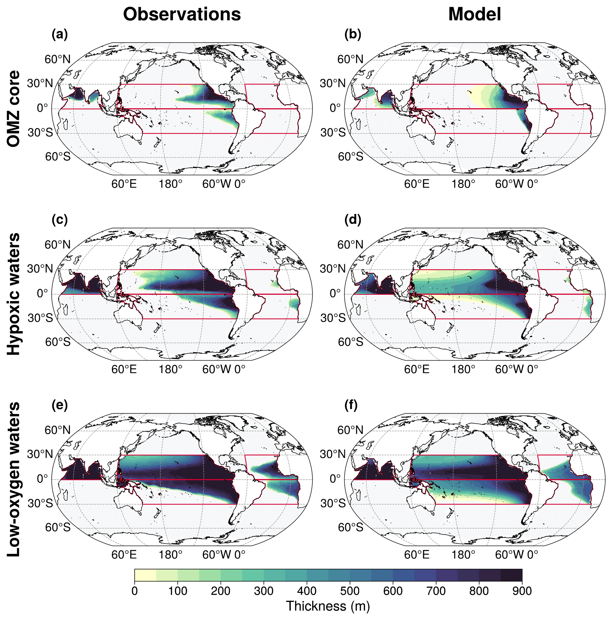
Figure 5 Comparison of 100–1000 m OMZ thickness between (a, c, d) the World Ocean Atlas climatology and (b, d, f) IPSL-CM6A-LR Large Ensemble mean. The thickness of the (a, b) OMZ core, (c, d) hypoxic volumes, and (e, f) low-oxygen volumes is computed using the volume percentiles defined in Table 1. Red boxes indicate the five OMZ regions analysed in the IPSL-CM6A-LR simulations: the tropical North Pacific, tropical South Pacific, tropical North Atlantic, tropical South Atlantic, North Indian.

2.4 Oxygen decomposition

To investigate the drivers of deoxygenation within the selected OMZ spatial boxes, we decompose changes in dissolved oxygen (O₂) concentrations into two components: the saturation concentration of oxygen (O_2sat) and the Apparent Oxygen Utilisation (AOU). This decomposition follows:

$$\begin{array}{}\text{(2)}& \mathrm{\Delta }{\mathrm{O}}_{\mathrm{2}}=\mathrm{\Delta }{\mathrm{O}}_{\mathrm{2}\mathrm{sat}}-\mathrm{\Delta }\mathrm{AOU}\end{array}$$

The saturation concentration O_2sat represents the oxygen solubility, which depends non-linearly on temperature and salinity. It is computed at each model grid point using monthly temperature and salinity fields and gsw-python package (Firing et al., 2021). The AOU reflects the net effect of biological oxygen consumption and physical ventilation of water masses. It is computed as the residual between modelled O₂ concentrations and their corresponding saturation values.

To further interpret AOU variations in the 100–1000 m depth range, we examine two key drivers: the carbon export flux at 100 m and the mean age since surface contact. The carbon export flux serves as a proxy for biological oxygen demand contributing to AOU, while the mean age reflects water masses ventilation.

All variables are extracted or computed prior to the application of the piControl drift correction and are subsequently detrended using the same method applied to the O₂ fields.

2.5 Time of emergence

We use the concept of time of emergence to detect climate-driven changes exceeding internal variability. The time of emergence is defined as the last time step at which the climate-forced signal becomes statistically distinguishable from internal variability, referred to as the noise (Hawkins and Sutton, 2012). This condition is formally expressed as:

$$\begin{array}{}\text{(3)}& \text{ToE}:{\displaystyle \frac{S}{N}}\ge \mathrm{2}\end{array}$$

where S represents the climate-driven signal and N represents the noise. A ratio of 2 corresponds to a confidence level of 95 %, ensuring that the detected emergence is robust (von Storch and Zwiers, 1999).

Each member within the IPSL Large Ensemble contains both the climate-driven signal and the system's internal variability (Deser et al., 2012). By conducting an ensemble of 30 experiments, we are able to separate these two components. The climate signal is estimated by averaging across ensemble members, while internal variability is quantified as the Large Ensemble standard deviation (Deser et al., 2012). For each biogeochemical variable and for each previously defined OMZ volume, climate-driven signals are extracted from anomalies, which are computed relative to the pre-industrial period (1850–1899). Internal variability is time dependent and estimated using absolute values rather than anomalies. Anomalies are calculated relative to the pre-industrial period for all Large Ensemble members, which eliminates the advantage of the different initial conditions in sampling the model’s internal variability. As a result, anomalies underestimate internal variability during the pre-industrial period. The use of time dependant internal variability is particularly relevant given that internal variability can evolve under climate change scenarios. It is particularly true in the IPSL-CM6A-LR large ensemble where the spread across ensemble members decreases under future forcing, reflecting the influence of anthropogenic external forcings on internal modes of variability (Bonnet et al., 2021).

Each ensemble member can also be interpreted as a distinct realisation of the climate response to the SSP2-4.5 scenario. Accordingly, we also compute the time of emergence for each individual simulation. In this case, the externally forced signal is taken from a single member, while the internal variability is still estimated using the ensemble standard deviation. This procedure yields a distribution of times of emergence across the ensemble.

3 Results

3.1 Climate-driven OMZ volume signals

Here, we present the ensemble mean climate-driven changes in OMZ core volumes, hypoxic volumes and low-oxygen volumes across each OMZ spatial domain, along with their corresponding time-dependent internal variability (Fig. 6). We also examine the time of emergence of the climate-driven volume signal, defined as the year when the forced signal exceeds twice the magnitude of time-dependent internal variability (Fig. 6, Table 2).

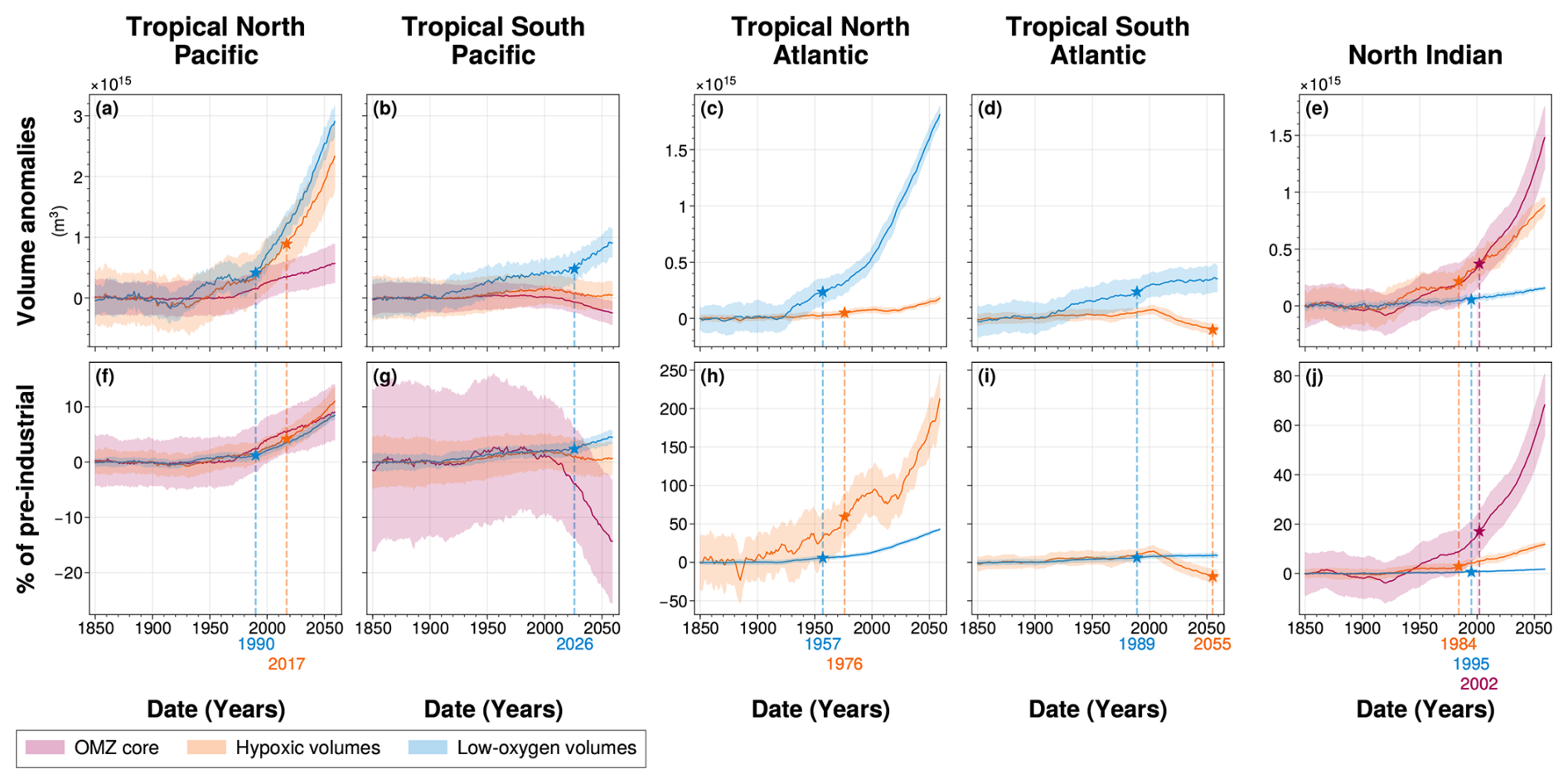
Figure 6 Time of emergence of 100–1000 m OMZ volumes for (a, f) the tropical North Pacific, (b, g) the tropical South Pacific, (c, h) the tropical North Atlantic, (d, i) the tropical South Atlantic and (e, j) the North Indian ocean. In all panels, colours represent the [O₂] threshold used to define OMZ volumes: (purple) OMZ cores, (orange) hypoxic volumes and (blue) low-oxygen volumes. The time of emergence, indicated by the symbol star in all panels, is the last time step at which (solid line) the Large Ensemble mean exceeds twice (coloured area) the Large Ensemble standard deviation. The time of emergence is calculated for the (a–e) OMZ volume anomalies relative to pre-industrial period (1850–1899) and (f–j) percentage of pre-industrial mean volume. All times of emergence are indicated on the bottom axis and summarized in the Table 2.

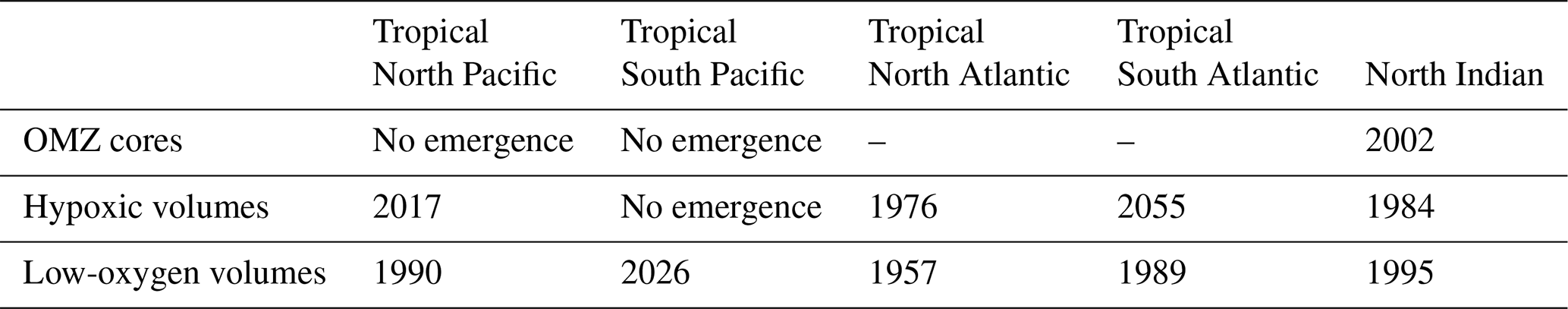
Table 2 Time of emergence of 100–1000 m OMZ volume anomalies for the Large Ensemble mean in each OMZ box. “No emergence” indicates that the ensemble mean has not emerged at the level of twice the ensemble standard deviation, across the IPSL Large Ensemble, by the end of the simulation (Fig. 6). The symbol “–” indicates the absence of OMZ core in the region of interest.

3.1.1 Evolution of climate-driven OMZ volume signals

Across all OMZ regions, low-oxygen volumes exhibit a clear and consistent expansion throughout the simulation (Fig. 6). This expansion is particularly pronounced in the tropical North Pacific and tropical North Atlantic, with total volume increases of 2.8×10¹⁵ and 1.8×10¹⁵ m³, respectively, by the end of the simulation (Fig. 6a and c). However, in all regions except the tropical North Atlantic, this expansion remains below 10 % of their pre-industrial mean volumes (Fig. 6f–j). Only the tropical North Atlantic low-oxygen volume shows a strong expansion, reaching 42 % increase relative to its pre-industrial mean (Fig. 6h).

In the South Atlantic, the expansion of low-oxygen waters slows during the SSP2-4.5 period (2015–2059), with a rate of 3.3×10¹² m³ yr⁻¹ compared to 5.4×10¹¹ m³ yr⁻¹ during the historical period (1970–2014) (Fig. 6c and h). Other OMZ regions exhibit a monotonic expansion under SSP2-4.5, with the tropical North Pacific growing at 4.2×10¹³ m³ yr⁻¹, the tropical North Atlantic at 2.3×10¹³ m³ yr⁻¹, the tropical South Pacific at 1.2×10¹³ m³ yr⁻¹, and the North Indian Ocean at 1.6×10¹² m³ yr⁻¹ (Fig. 6a, b, c, and e).

In the tropical North Pacific and tropical North Atlantic, hypoxic volumes also expand (Fig. 6a and c). In the tropical North Pacific, the hypoxic volume increases by 2.3×10¹⁵ m³, corresponding to a 11 % increase relative to its pre-industrial mean. The tropical North Atlantic only increases by 1.7×10¹⁴ m³ but exhibits the largest relative increase of 197 % by the end of the simulation as it has the smallest hypoxic volume among the IPSL Large Ensemble’s present-day climatology. These expansions result from increasing rates during the SSP2-4.5 period (2015–2059) of 3.3×10¹³ m³ yr⁻¹ in the tropical North Pacific and 2.5×10¹² m³ yr⁻¹ in the tropical North Atlantic, and corresponding to annual increases of 0.15 % and 3.0 % of their pre-industrial mean volumes (Fig. 6a, c, f, and h). Expansion during SSP2-4.5 is substantially stronger than in the present-day period (1970–2014), with growth rates increasing by factors of 2.4 and 3.6, respectively (Fig. 6a and c).

Hypoxic volumes in the tropical South Pacific and tropical South Atlantic shift from a weak expansion to a contraction trend in about 2004 with contraction rates during SSP2-4.5 of 1.7×10¹² and 2.9×10¹² m³ yr⁻¹, respectively (Fig. 6b, d and Table A1). The contraction in the tropical South Atlantic is particularly marked, exceeding the preceding expansion rate and resulting in a 18 % reduction in hypoxic volume relative to pre-industrial levels. Meanwhile, the tropical South Pacific hypoxic volume shows no statistically significant net change at the end of the simulation.

OMZ core volumes show divergent trends between regions. In the tropical North Pacific and tropical North Indian Ocean, they expand slowly in the former (5.2×10¹² m³ yr⁻¹) with a total increase of 9 % by the end of the simulation, and more substantially in the latter (2.1×10¹³ m³ yr⁻¹) with a total increase of 68 % by the end of the simulation (Fig. 6a, e, and j). Conversely, the OMZ core in the tropical South Pacific shows a strong contraction resulting in a 14 % volume reduction at the end of the simulation which correspond to a contraction rate of 5.5×10¹² m³ yr⁻¹ during the SSP2-4.5 period (Fig. 6b and g).

3.1.2 OMZ volume variability

The Internal variability is quantified by the Large Ensemble standard deviation of OMZ volumes (Fig. 6). In both the tropical North and South Pacific, internal variability of OMZ volumes is higher than in the other regions with maximum Large ensemble standard deviation for the hypoxic volumes in the tropical North Pacific ($\mathrm{4}.\times {\mathrm{10}}^{\mathrm{14}}$ m³) and minimum for the tropical South OMZ core (2.1×10¹⁴ m³) (Fig. 6a and b). Thus, in the tropical Pacific, internal variability is of comparable magnitude across all OMZ volume classes, despite differences in Large Ensemble mean absolute volume (Fig. 6a and b). The tropical Atlantic shows the lowest Large Ensemble standard deviation, thus the lowest internal variability, with hypoxic and low-oxygen volumes varying by 2.3×10¹³ and 1.2×10¹⁴ m³, respectively. In the North Indian Ocean, hypoxic and OMZ core volumes exhibit greater mean variability (1.3×10¹⁴ and 1.9×10¹⁴ m³, respectively) compared to low-oxygen volumes (2.7×10¹³ m³).

Over the SSP2-4.5 period (2014–2060), OMZ volumes in the Tropical South Pacific and Tropical North Pacific, as well as hypoxic and low-oxygen volumes in the North Indian Ocean, exhibit a decrease in the Large Ensemble standard deviation relative to their pre-industrial (1850–1900) mean value. The reduction reaches 40 % for hypoxic volume in the Tropical South Pacific and low-oxygen volume in the Tropical North Pacific, and about 50 % in the North Indian Ocean (Fig. A2g, h, and j). Over the same period, only the OMZ core volume in the North Indian Ocean shows an increase in the Large Ensemble standard deviation, of about 60 % (Fig. A2j). All other OMZ volumes display a standard deviation that remains within 20 % of their respective pre-industrial values (Fig. A2).

3.1.3 Time of emergence of climate-driven OMZ volume signals

With the exception of the North Indian Ocean, the climate-driven signal in low-oxygen volumes emerges from internal variability earlier than in the other types of OMZ volumes, making it the earliest detectable signal of change in all OMZ regions. Emergence of this signal occurs as early as 1957 in the tropical North Atlantic, followed by 1989 in the tropical South Atlantic, 1990 in the tropical North Pacific, and 2026 in the tropical South Pacific (Fig. 6a–d, Table 2). These timings reveal a hemispheric asymmetry: the signal emerges 36 years earlier in the tropical North Pacific than in the tropical South Pacific, and 32 years earlier in the tropical North Atlantic than in the tropical South Atlantic (Fig. 6a–c, Table 2). However, emergence in the tropical North Atlantic leads that of the tropical North Pacific by 33 years (Fig. 6a and c, Table 2). In the North Indian Ocean, however, although all three volume categories show detectable climate-driven signals emergence before the end of the simulation; the low-oxygen volume climate-driven signal emerges in 1995 (Fig. 6e).

In both the tropical Pacific and tropical Atlantic, the climate-driven signal expansions in hypoxic volumes either emerge later than in low-oxygen volumes or do not emerge at all within the 210 year simulation period. In the tropical North Atlantic and tropical North Pacific, emergence occurs in 1976 and 2017, respectively (Fig. 6a and c, Table 2). In the tropical South Atlantic, although the signal initially follows a slow expansion, a sharp reversal leads to contraction, with emergence detected in 2055 (Fig. 6a and c, Table 2). By contrast, the hypoxic volume signal in the tropical South Pacific does not emerge before the end of the simulation with no statistically significant changes compared to pre-industrial era (Fig. 6a and c, Table 2). In the North Indian Ocean, hypoxic volume expands and the climate-driven signal emerges from internal variability in 1984 (Fig. 6e, Table 2).

In both the tropical North and South Pacific, although the OMZ core volumes expand and contract, respectively, the climate signal does not exceed twice the range of internal variability, and therefore does not emerge within the simulation period. In the North Indian Ocean, the OMZ core forced signal emerges in 2002 (Fig. 6e, Table 2).

3.2 Deoxygenation and its drivers in each OMZ spatial domains

Here, we present climate-driven changes in mean dissolved oxygen concentration and its associated drivers (O_2sat and AOU) across each OMZ spatial domain, along with their corresponding time-dependent internal variability (Fig. 7). We also examine the time of emergence of these climate-driven signals, defined as the year when the forced signal exceeds twice the magnitude of time-dependent internal variability, quantified here as the Large Ensemble standard deviation (Fig. 7, Table 3).

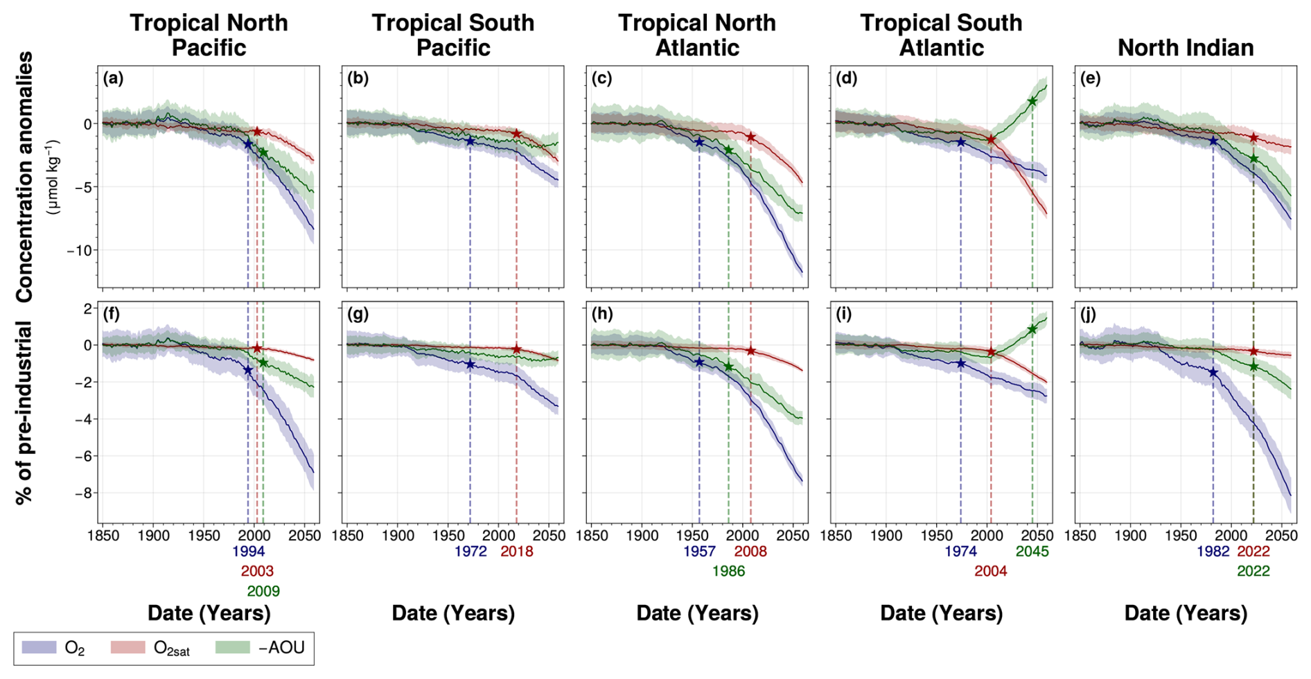
Figure 7 Time of emergence of 100–1000 m spatial mean concentrations of (blue) O₂, (red) O_2sat and (green) −AOU in the IPSL Large Ensemble for (a, f) the tropical North Pacific, (b, g) the tropical South Pacific, (c, h) the tropical North Atlantic, (d, i) the tropical South Atlantic and (e, j) the North Indian ocean. The time of emergence (indicated by the star symbol) is defined as the last point at which (a–e) the Large Ensemble mean concentration anomalies, and (f–j) the Large Ensemble mean percentage of pre-industrial concentrations exceed twice (coloured areas) their respective Large Ensemble standard deviations.

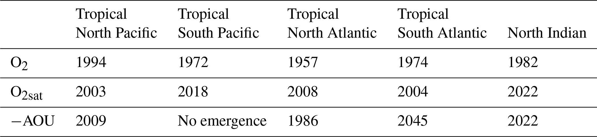
Table 3 Time of emergence of 100–1000 m spatial mean concentration anomalies for the Large Ensemble mean in each OMZ box. “No emergence” indicates that the ensemble mean has not emerged from twice the ensemble standard deviation, across the IPSL Large Ensemble, by the end of the simulation (Fig. 7).

All OMZ regions exhibit a decline in mean dissolved oxygen concentrations throughout the simulation (Fig. 7). The northern parts of the tropical Pacific and tropical Atlantic OMZs show the most pronounced deoxygenation, with decreases in dissolved oxygen concentration of 8.1 and 12 µmol kg⁻¹, respectively, by the end of the simulation (Fig. 7a and c). These losses are greater than in the southern hemisphere OMZs of the same basin, which decline by 4.4 µmol kg⁻¹ in the tropical Pacific and 4.0 µmol kg⁻¹ in the tropical Atlantic (Fig. 7b and d). With the exception of the tropical South Atlantic, all regions experience an acceleration in deoxygenation during the SSP2-4.5 period (2014–2059) compared to the present-day period (1970–2014) (Fig. 7). In the tropical South Atlantic, however, deoxygenation follows a nearly linear trend, with a present-day rate of 0.035 $\mathrm{\mu }\mathrm{mol}{\mathrm{kg}}^{-\mathrm{1}}{\mathrm{yr}}^{-\mathrm{1}}$ and a slightly slower rate of 0.029 $\mathrm{\mu }\mathrm{mol}{\mathrm{kg}}^{-\mathrm{1}}{\mathrm{yr}}^{-\mathrm{1}}$ during SSP2-4.5. During the SSP2-4.5 period, oxygen loss is more severe in the Northern Hemisphere OMZ regions: the tropical North Pacific experiences deoxygenation at twice the rate of the tropical South Pacific, and the tropical North Atlantic at more than five times the rate of the tropical South Atlantic (Fig. 7f–i). The North Indian Ocean undergoes the greater oxygen decline of all regions, with an 8.1 % reduction relative to its pre-industrial mean by the end of the simulation (Fig. 7j).

In all regions, the climate-driven deoxygenation signal emerges from internal variability before the end of the simulation period (Fig. 7, Table 3). These signals emerge after the mid-20th century in all regions and before 21st century, beginning in the tropical North Atlantic in 1957, followed by the tropical South Pacific and South Atlantic in 1972 and 1974, respectively, then the North Indian Ocean in 1982, and finally the tropical North Pacific in 1994 (Fig. 7, Table 3).

Decomposition of the oxygen signal into contributions from oxygen solubility (O_2sat) and apparent oxygen utilisation (−AOU) reveals contrasting dynamics. A decrease in O_2sat emerges in all regions during the first quarter of the 21st century, while the −AOU signal shows regionally divergent trends: it declines and exceeds their internal variability in the North Pacific, North Atlantic, and North Indian Ocean, but increases in the tropical South Atlantic and the tropical South Pacific (Fig. 7, Table 3).

In all regions, O_2sat emerges after deoxygenation (Fig. 7, Table 3). Both O₂ and O_2sat decline gradually until about 2000, after which the decline accelerates sharply and continues to decrease throughout the simulation period (Fig. 7a–e). In all regions, the decline rate increases by a factor 10 between the periods before and after around 2004 (Fig. 7a–e and Table A1). Emergence occurs close to or shortly after this regime shift: in 2003 in the North Pacific, 2004 in the South Atlantic, 2008 in the North Atlantic, 2018 in the South Pacific, and 2022 in the North Indian Ocean (Fig. 7, Table 3). The acceleration is accompanied by a reduction in signal variability, consistent with emergence occurring near the regime shift (Fig. 7).

Although all OMZ regions display a consistent trend of deoxygenation and O_2sat decline, the −AOU component shows contrasting behaviours between hemispheres. In the tropical North Pacific and tropical North Atlantic, −AOU decreases by 5.3 and 7.1 µmol kg⁻¹, respectively, by the end of the simulation (Fig. 7a and c). The emergence of this signal occurs later in the tropical North Pacific (2009) than in the tropical North Atlantic (1986) (Fig. 7a and c, Table 3). By contrast, the tropical South Atlantic initially exhibits a slow decrease in −AOU at a rate of $\mathrm{5.0}\times {\mathrm{10}}^{-\mathrm{3}}$ $\mathrm{\mu }\mathrm{mol}{\mathrm{kg}}^{-\mathrm{1}}{\mathrm{yr}}^{-\mathrm{1}}$, followed by a sharp increase after 2004 at a rate of 0.086 $\mathrm{\mu }\mathrm{mol}{\mathrm{kg}}^{-\mathrm{1}}{\mathrm{yr}}^{-\mathrm{1}}$ (Table A1). This reversal results in a total increase of 2.8 µmol kg⁻¹ by the end of the simulation. The positive −AOU anomalies in this region become distinguishable from internal variability in 2045 (Fig. 7b and d, Table 3). In the tropical South Pacific, the −AOU signal does not show a distinct regime shift point but shows a slower decreasing trend during SSP2-4.5 period, with a rate of $\mathrm{6.7}\times {\mathrm{10}}^{-\mathrm{3}}$ $\mathrm{\mu }\mathrm{mol}{\mathrm{kg}}^{-\mathrm{1}}{\mathrm{yr}}^{-\mathrm{1}}$, compared to 0.011 $\mathrm{\mu }\mathrm{mol}{\mathrm{kg}}^{-\mathrm{1}}{\mathrm{yr}}^{-\mathrm{1}}$ before 2004. In the North Indian Ocean, −AOU follows a decreasing trajectory, with its signal emerging concurrently with that of O_2sat in 2022 (Fig. 7e, Table 3).

3.3 Biological and ventilation dynamics

Here, we present the ensemble-mean climate-driven changes in mean carbon export at 100 m and mean age since surface contact across each OMZ spatial domain, along with their corresponding time-dependent internal variability (Fig. 8). We also examine the time of emergence of these climate-driven signals, defined as the year when the forced signal exceeds twice the magnitude of internal variability (Fig. 8).

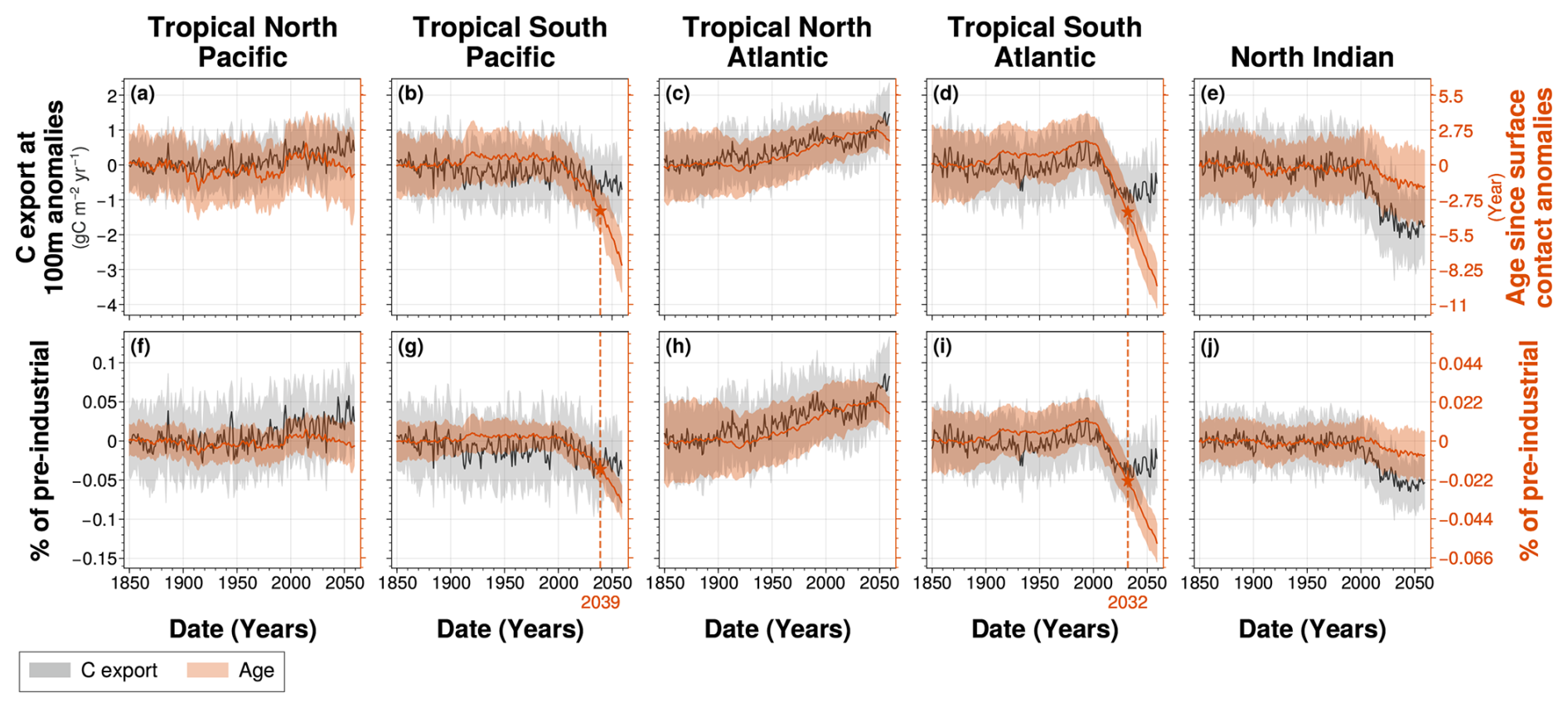
Figure 8 Spatial mean of (grey) carbon export anomalies at 100 m depth and (orange) age since surface contact anomalies between 100 and 1000 m depth for (a, f) the tropical North Pacific, (b, g) the tropical South Pacific, (c, h) the tropical North Atlantic, (d, i) the tropical South Atlantic and (e, j) the North Indian ocean. Solid lines represent (a–e) the Large Ensemble mean anomalies relative to pre-industrial period (1850–1900) and (f–j) the percentage of pre-industrial mean, while the shaded areas correspond to their respective Large Ensemble standard deviation within the IPSL Large Ensemble. Star symbols indicate the time of emergence, defined as the last point at which (solid lines) the Large Ensemble mean exceeds twice (coloured areas) the Large Ensemble standard deviation.

By disentangling the effects of biological activity and ventilation, the abrupt shift in the −AOU signal at about 2004 in the tropical North Atlantic coincides with simultaneous changes in both carbon export and water mass age (Fig. 8).

Before 2004, carbon export remains stable across all OMZ regions, except in the tropical North Atlantic, where it increases at $\mathrm{9.4}\times {\mathrm{10}}^{-\mathrm{3}}$ $\mathrm{g}\mathrm{C}{\mathrm{m}}^{-\mathrm{2}}{\mathrm{yr}}^{-\mathrm{1}}$ (Fig. 8a–e and Table A1). The North Indian Ocean shows the highest mean carbon export before 2004, with an export rate of 3.3 $\mathrm{g}\mathrm{C}{\mathrm{m}}^{-\mathrm{2}}{\mathrm{yr}}^{-\mathrm{1}}$. Tropical Pacific and tropical Atlantic OMZ regions exhibit a hemispheric asymmetry. The carbon export rates are higher in the southern hemisphere OMZ regions, with values of 1.9 $\mathrm{g}\mathrm{C}{\mathrm{m}}^{-\mathrm{2}}{\mathrm{yr}}^{-\mathrm{1}}$ in the tropical South Pacific and 2.3 $\mathrm{g}\mathrm{C}{\mathrm{m}}^{-\mathrm{2}}{\mathrm{yr}}^{-\mathrm{1}}$ in the tropical South Atlantic, than in the northern hemisphere OMZs of the same basin, which have an export of 1.6 and 1.8 $\mathrm{g}\mathrm{C}{\mathrm{m}}^{-\mathrm{2}}{\mathrm{yr}}^{-\mathrm{1}}$, respectively. After 2004, a pronounced decline in carbon export is observed over approximately two decades in the North Indian Ocean, tropical South Atlantic, and tropical South Pacific, before stabilising toward the end of the simulation (Fig. 8b, d, and e). The cumulative decline in carbon export over this period reaches 1.7 $\mathrm{g}\mathrm{C}{\mathrm{m}}^{-\mathrm{2}}{\mathrm{yr}}^{-\mathrm{1}}$ in the North Indian Ocean, 0.63 $\mathrm{g}\mathrm{C}{\mathrm{m}}^{-\mathrm{2}}{\mathrm{yr}}^{-\mathrm{1}}$ in the tropical South Atlantic, and 0.70 $\mathrm{g}\mathrm{C}{\mathrm{m}}^{-\mathrm{2}}{\mathrm{yr}}^{-\mathrm{1}}$ in the tropical South Pacific. By contrast, the tropical North Atlantic exhibits stable carbon export during this period, followed by a continued gradual increase at a rate similar to that observed before 2004 (Fig. 8d). Meanwhile, the tropical North Pacific shows a steady post-2004 increase in carbon export, at $\mathrm{4.6}\times {\mathrm{10}}^{-\mathrm{3}}$ $\mathrm{g}\mathrm{C}{\mathrm{m}}^{-\mathrm{2}}{\mathrm{yr}}^{-\mathrm{1}}$ (Fig. 8c and Table A1).

Before 2004, the age since surface contact shows no statistically significant variations in any OMZ regions, except in the tropical North Atlantic, where it begins increasing in 1925 at a steady rate of $\mathrm{3.8}\times {\mathrm{10}}^{-\mathrm{2}}$ yr yr⁻¹, continuing through the end of the simulation (Fig. 8a). The tropical Pacific exhibits the highest mean age since surface contact before 2004, with values of 263 years in the tropical North Pacific and 227 years in the tropical South Pacific. The tropical Atlantic shows lower values, with 122 years in the tropical North Atlantic and 166 years in the tropical South Atlantic. After 2004, the age since surface contact decreases sharply in the tropical Southern Hemisphere OMZ regions, with total reductions of 7.3 years in the tropical South Pacific and 9.0 years in the tropical South Atlantic by the end of the simulation. These represent declines of 3.2 % and 5.4 % relative to their respective pre-industrial means. The corresponding rates of decline are 0.20 yr yr⁻¹ in the tropical South Atlantic and 0.15 yr yr⁻¹ in the tropical South Pacific (Fig. 8b and d). A slower decline is also observed in the North Indian Ocean, with a rate of 0.028 yr yr⁻¹ (Fig. 8e). These changes lead to the emergence of the ventilation signal from internal variability in 2032 in the tropical South Atlantic and in 2039 in the tropical South Pacific. In the tropical North Pacific, the age since surface contact also begins to decline around 2004, although at a slower rate of 0.040 yr yr⁻¹ (Fig. 8c).

3.4 Time of Emergence distribution within the IPSL-CM6A-LR Large Ensemble

Here, we present the ensemble distribution of the time of emergence of climate-driven changes in mean dissolved oxygen concentration and OMZ volumes across each OMZ spatial domain (Fig. 9). We show the corresponding boxplots, along with the time of emergence and associated trend sign for each ensemble member (Fig. 9).

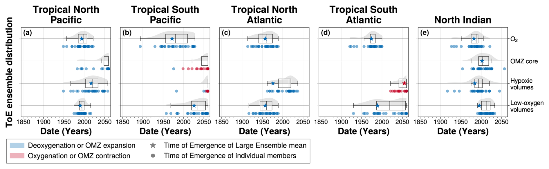
Figure 9 Distribution of the time of emergence within the IPSL Large Ensemble for (a) the tropical North Pacific, (b) the tropical South Pacific, (c) the tropical North Atlantic, (d) the tropical South Atlantic and (e) the North Indian ocean. Time of emergence is computed for 100–1000 m (first row) spatial mean concentration anomalies of O₂ and OMZ volume anomalies for (second row) OMZ core, (third row) hypoxic volumes and (fourth row) low-oxygen volumes. In all panels, the box plots illustrate the dispersion of the time of emergence around the median across the IPSL Large Ensemble, while the violin plots illustrate the distribution of the time of emergence within the IPSL Large Ensemble. The star symbol represents the time of emergence for the Large Ensemble mean, defined as the last time at which it exceeds twice the Large Ensemble standard deviation. The dots represent the time of emergence of individual ensemble members signal, defined as the last time at which each member individually exceeds twice the Large Ensemble standard deviation. Their colours indicate the sign of their trend at the emergence: blue for deoxygenation or OMZ expansion, and red for oxygenation or OMZ contraction.

For OMZ volumes and dissolved oxygen concentrations, the sign of the trend at the time of emergence of the ensemble mean is further supported by the emergence of individual ensemble members (Fig. 9). In cases where the Large Ensemble mean does not emerge by the end of the simulation, some individual members nonetheless show emergence. They correspond to members exhibiting stronger variability around the externally forced trend, and thereby corroborate the trend direction of the ensemble mean. This is particularly evident in the tropical South Pacific and tropical South Atlantic, where individual members exhibit clear emergence of OMZ core and hypoxic volume contraction (Fig. 9b and d).

Across all OMZ regions, the ensemble mean time of emergence is generally earlier than the ensemble median, with large spread quantified by the interquartile range (Fig. 9). The North Indian Ocean stands out as the only region where all metrics (dissolved oxygen concentrations and OMZ volumes) exhibit a narrow emergence window, with spreads limited to 17 years for oxygen signal and 25 years for OMZ core volumes (Fig. 9e). In other regions, broader spreads are linked either to weaker trend magnitudes at the time of emergence, as in the tropical South Pacific where deoxygenation shows an interquartile range of 54 years, or to regime shifts that change the trend sign, such as in the tropical South Atlantic where the low-oxygen volume signal displays a 71 year spread (Fig. 9b and d).

In all regions except the North Indian Ocean, the ensemble mean for dissolved oxygen concentration emerges earlier than, or concurrently with, the low-oxygen volume ensemble mean (Fig. 9). However, due to the large spread among members in time of emergence, the distributions of deoxygenation and OMZ volumes time of emergence overlap in all regions (Fig. 9).

4 Discussion

4.1 Emerging low-oxygen volume expansion in OMZ

Among the three OMZ regimes, only the low-oxygen volume exhibits a consistent expansion with a detectable emergence of the climate-driven signal from internal variability across all OMZ regions (Fig. 6). This result is consistent with the findings of Ditkovsky et al. (2023), who showed that OMZ volumes defined using higher oxygen thresholds expand across all OMZ regions. A comparison of their time of emergence also reveals regional offsets between ocean basins. Specifically, the tropical Atlantic OMZ shows an earlier emergence, by approximately two to three decades, compared to the tropical Pacific OMZ (Fig. 10). This earlier emergence is not due to faster expansion, but rather to lower internal variability of the tropical Atlantic low-oxygen volumes, which makes the climate-driven trend detectable before the tropical Pacific low-oxygen volumes expansion (Fig. 6).

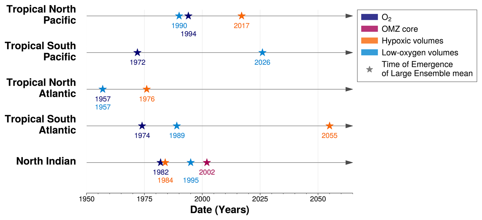
Figure 10 Time of Emergence of Large Ensemble mean for (rows) each OMZ box. The time of emergence, represented by the star symbol, is computed for 100–1000 m (dark blue) spatial mean concentration anomalies of O₂ and OMZ volume anomalies for (purple) OMZ core, (orange) hypoxic volumes and (light blue) low-oxygen volumes.

Although low-oxygen volumes expand in all OMZ regions, subdividing the tropical Pacific and tropical Atlantic OMZs into northern and southern subregions reveals a consistent 30 year delay in the emergence of low-oxygen volumes in the Southern Hemisphere compared to the Northern Hemisphere (Fig. 10). While internal variability remains similar across hemispheres within each basin, the magnitude of the climate-driven trend is stronger in the Northern Hemisphere in both basins (Fig. 6). A similar hemispheric asymmetry is observed in the mean deoxygenation trends, where climate-driven declines in oxygen concentrations are stronger in the northern hemisphere OMZs than in the southern hemisphere OMZs of the same basin (Fig. 7).

Low-oxygen volumes are critical as they influence the distribution of habitable zones for many marine species (Bertrand et al., 2011). In the IPSL-CM6A-LR model, the emergence of tropical Atlantic low-oxygen volumes occurs earliest, impacting oxygen-dependent ecosystem sooner than in other OMZ regions. Moreover, the expansion of low-oxygen waters is stronger in the Northern Hemisphere than in the Southern Hemisphere, leading to uneven impacts on marine ecosystems between hemispheres.

Moreover, the hemispheric asymmetry implies a stronger expansion of low-oxygen waters in the Northern Hemisphere than in the Southern Hemisphere, leading to uneven impacts on marine ecosystems between the two hemispheres.

4.2 Inter-hemispheric contrast in emerging OMZ core and hypoxic volume change

The north-south subdivision of the OMZs shows asymmetric dynamics between the North and South parts of the OMZs. The core of the OMZs only expands in the northern hemisphere by the end of the simulation while they are shrinking in the southern hemisphere OMZs of the same basin (Fig. 6). The tropical South Pacific and tropical South Atlantic OMZs show a contraction of their volume with lowest oxygen concentration, the OMZ core in the former and hypoxic waters in the latter, which is consistent with the findings of Busecke et al. (2022); Ditkovsky et al. (2023) (Fig. 6). In both tropical Pacific and tropical Atlantic, the southern OMZ core is being ventilated by younger water masses (Figs. 7 and 8). This is consistent with the single-pipe and mixing network ventilation framework developed by Gnanadesikan et al. (2007, 2012). It suggests that in a warmer and more stratified ocean, the proportion of different ventilation sources shifts, favouring younger subsurface waters. In the tropical South Atlantic, ventilation is provided by younger subsurface waters originating from the South Indian Ocean, which are advected into the South Atlantic via the Agulhas Current (De Ruijter et al., 1999). In the tropical South Pacific, ventilation occurs through water masses from the southern Pacific basin, which are advected northward by the Humboldt Current. This ventilation process is co-located with southern OMZ core location in the geographic-space (Figs. 8 and A3). This oxygenation trend in the tropical South Atlantic basin is also exhibited by CMIP6 multi-model mean over the present-day period in Takano et al. (2023) and by the end of the 21st century over SSP1-2.6 and SSP5-8.5 in Kwiatkowski et al. (2020).

Unlike previous findings by Ditkovsky et al. (2023), our results do not show a contraction of the OMZ core in the North Indian Ocean. This discrepancy likely stems from misrepresentation of oxygen concentrations and deoxygenation patterns in the IPSL-CM6A-LR model. The Large Ensemble simulations of the IPSL model misrepresent oxygen levels in the North Indian, failing to capture the low-oxygen conditions observed in the Arabian Sea (Fig. 2). This bias is partly attributable to an overestimation of oxygen concentrations in marginal seas (the Persian Gulf and the Red Sea), combined with poorly constrained outflow parametrisations and a ventilation of the Arabian Sea OMZ by Southern Ocean water masses, where oxygen levels are overestimated (Schmidt et al., 2021). Furthermore, the model fails to reproduce the specific spatial patterns of oxygenation and deoxygenation identified in Ditkovsky et al. (2023) (Fig. 3). Specifically, Ditkovsky et al. (2023) describe a distinct dipole structure with an oxygenation pool between 10° N and 10° S along the western boundary, and a deoxygenation pool between 10 and 30° S along the eastern boundary. This dipole structure supports a double-pipe ventilation mechanism within the North Indian basin. The IPSL-CM6A-LR model simulates a broad deoxygenation trend across the basin and fails to capture this ventilation pattern (Fig. 3).

4.3 Time of emergence of regional deoxygenation relative to OMZ volumes

In the IPSL Large Ensemble, the OMZ regions mean deoxygenation signals emerges from natural variability before the end of the 20th century (Fig. 10). However, tropical Pacific and tropical Atlantic OMZs exhibit an asymmetry in the relative timing of emergence between deoxygenation and OMZ volume signals (Fig. 10). In the tropical North Pacific and tropical North Atlantic, the emergence of deoxygenation coincides with the expansion of low-oxygen volumes (Fig. 10). In these regions, regional mean deoxygenation provides an indicator of OMZ boundaries expansion, with implications for the distribution of marine ecosystems. In the southern parts of the tropical Pacific and tropical Atlantic OMZs, the regional mean climate-driven deoxygenation signals emerge earlier than the expansion of low-oxygen and other OMZ volumes (Fig. 10). Hypoxic waters, which are harmful or lethal to many marine organisms, emerge later than mean deoxygenation, with delays of 27 years in the tropical North Pacific and 19 years in the tropical North Atlantic (Fig. 10).

Although the emergence of regional mean dissolved oxygen captures the regional-scale evolution of low-oxygen waters in IPSL simulations, the emergence of local oxygen trends exhibits temporal heterogeneity. Consistent with the multi-model analysis of Hameau et al. (2020), who computed time of emergence at each grid point using CMIP5 models under the RCP8.5 scenario (Moss et al., 2010), the IPSL-CM6A-LR spatial median of local emergence occurs later than the regional mean deoxygenation signal in each OMZs regions (Fig. A3, Table A2). Except for the tropical North Atlantic, where the median emergence occurs in 1983, spatial median emergence times are in the first half of the 21st century (Table A2). This is consistent with Hameau et al. (2020), who exhibited a global mean oxygen emergence in 2019 for the CMIP5 IPSL-CM5A-LR model. Within OMZ regions, local emergence times shows a standard deviations ranging from 7 to 24 years (Fig. A3, Table A2). This is consistent with results of Long et al. (2016), who used the Community Earth System Model large ensemble (CESM Large Ensemble, Kay et al., 2015) under RCP8.5 to assess local deoxygenation time of emergence. The standard deviation of time of emergence within the OMZ regions reflects the delay of emergence between the three OMZ volumes of interest.

4.4 Sensitivity of the time of emergence of OMZ volumes to the reference period

In this study, we determine the emergence of OMZ volumes relative to pre-industrial using the IPSL-CM6A-LR model. Model simulations provide access to a pre-industrial baseline that is not available in current observational records, making it possible to characterise the full magnitude of climate-driven changes. However, observational oxygen datasets, such as the IAP dataset (Cheng and Gouretski, 2023), only cover the period from 1960 to the present and contain limited data within OMZs. As a result, using these datasets would only allow us to determine the emergence of deoxygenation and reconstructed OMZ volumes relative to the 1960–1970 period. The IPSL Large Ensemble simulations allow us to adopt the 1960–1970 period as a reference to compute time of emergence, providing an estimate of when climate-driven signals in OMZ volumes may become detectable using observation datasets. Using the same method as our previous analysis, times of emergence of dissolved oxygen and OMZ volumes anomalies are computed relative to the 1960–1970 period for both the ensemble mean and individual members. Internal variability is estimated by the Large Ensemble standard deviation.

Except for the hypoxic volume in the South Atlantic, all time of emergence distributions shift towards later emergence times, with the ensemble-mean emergence delayed by up to 59 years (Fig. A5). However, all ensemble-mean signals that emerged with a pre-industrial reference also emerge before the end of the simulation (2059) when the 1960–1970 reference is used (Fig. A5). Thus the climate-driven emergence of OMZ volumes is ongoing, although it remains challenging to detect in observations. The detection challenge arises from the difficulty of measuring OMZ volumes and accurately estimating their natural variability, which is entangled with their anthropogenic response.

4.5 Limitations

The IPSL-CM6A-LR model exhibits a positive bias in dissolved oxygen concentrations, particularly in the OMZ regions. This oxygen overestimation in tropical OMZs is linked to the IPSL-CM6A-LR coarse spatial resolution, which leads to weaker equatorial currents (Busecke et al., 2019; Calil, 2023). To assess large-scale physical ventilation, we compare age since surface contact at the end of the piControl simulation (years 3840–3850) with two data-driven inverse models: the Total Matrix Intercomparison (TMI) and the Ocean Circulation Inverse Model (OCIM) (Millet et al., 2025). The IPSL model reproduces shadow zones in the tropical regions of interest, indicating the representation of large-scale physical ventilation of tropical regions (Fig. A4). The oxygen overestimation is then also linked to too strong deep convection in the Southern Ocean (Boucher et al., 2020). Thus we used fixed-percentile approach, rather than fixed-threshold approach, to define OMZ volumes derived from the WOA observational product.

However, this approach does not correct for biases inherent to WOA18, which is known to underestimate hypoxic volumes (Bianchi et al., 2012; Kwiecinski and Babbin, 2021). To account for these uncertainties, we evaluate the sensitivity of our results to alternative OMZ definitions (fixed-threshold versus fixed-percentile), such that the resulting range of responses encompasses uncertainties from IPSL oxygen overestimation and WOA18 underestimation of OMZ volumes (Fig. A6). The sign of the climate-driven emergence trends are consistent across both definitions (Fig. A6e–j). However, the percentile-based approach allows to detect the emergence of OMZ core and hypoxic volume signals, where the fixed-threshold method fails (Fig. A6e–j). This reflects the fact that the classical method underestimates or misses the climate-driven signal due to the biased baseline in oxygen levels. The time of emergence of low-oxygen volumes is relatively insensitive to the OMZ definition used, reflecting the smaller oxygen bias at higher concentrations in IPSL-CM6A-LR (Fig. A6k–o).

The time of emergence is highly sensitive to the representation and the quantification of the internal variability of the signal of interest (Hameau et al., 2019). In this study, internal variability was measured by the standard deviation of the IPSL Large Ensemble. The 2000 years piControl simulation provides an alternative estimate of internal variability, capturing decadal to millennial fluctuations. However, as it is conducted under pre-industrial forcing conditions, it does not account for changes in internal variability induced by historical and SSP2-4.5 forcing.

To evaluate the impact of the variability measure, we computed time of emergence using, for the noise term, the Large Ensemble standard deviation and the constant standard deviation derived from the full piControl simulation. The emergence the ensemble mean signal is not substantially affected by the choice of variability estimate (Fig. A7). However, when internal variability is estimated from the piControl simulation, the emergence distribution across ensemble members shifts towards later times (Fig. A7). Consistent with previous findings of Hameau et al. (2019) using the CESM1 model under the RCP8.5 scenario, piControl-based variability tends to overestimate internal variability, resulting in a later time of emergence.

5 Conclusions

We used the IPSL-CM6A-LR Large Ensemble to explore how climate-driven deoxygenation affects OMZ. We find that the mean deoxygenation trend primarily reflects the expansion of OMZ low-oxygen waters. This expansion emerges as a climate-driven signal at the same time as the mean deoxygenation trend in OMZ areas. By contrast, OMZ cores do not expand. Instead, they contract, delaying their emergence. This contraction is particularly evident in the Southern Hemisphere, where oxygen concentrations are maintained by physical ventilation associated with a decrease in water-mass age. This is consistent with the findings of Gnanadesikan et al. (2007, 2012), which highlight the importance of extra-tropical ventilation pathways in controlling the ventilation of OMZ cores. As a result, OMZ core volumes do not emerge from internal variability before the end of the simulation. Overall, our findings suggest that climate-driven deoxygenation is already reshaping OMZ volumes and climate-driven expansions of OMZ volumes are already emerging from natural variability, with consequences for marine ecosystems.

Appendix A

A1 Comparison between models and observations

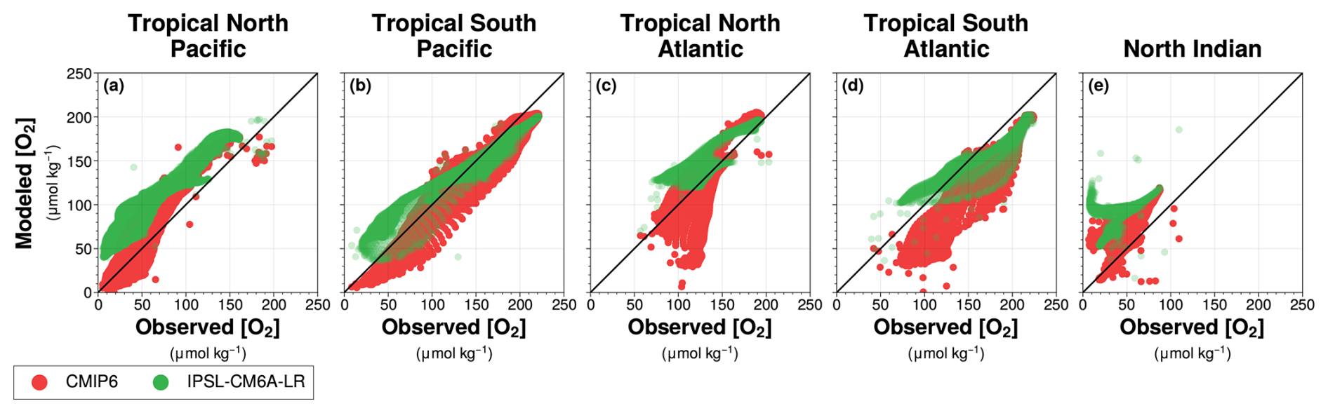
Figure A1 Dissolved oxygen concentrations from the World Ocean Atlas 2018 compared with dissolved oxygen concentrations simulated by the (green) IPSL-CM6A-LR Large Ensemble mean and the (red) CMIP6 multi-model mean. Values are taken from each grid point between 100–1000 m depth for (a) the tropical North Pacific, (b) the tropical South Pacific, (c) the tropical North Atlantic, (d) the tropical South Atlantic and (e) the North Indian Ocean. The black solid line indicates the identity function (y=x).

A2 Climate-driven trends

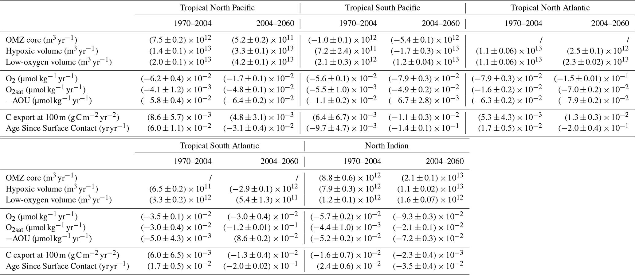
Table A1 Climate-driven trends of OMZ volumes and biogeochemical variables of interest. Trends are evaluated before (1970–2004) and after (2004–2060) the regime shift identified in the biogeochemical variables of IPSL-CM6A-LR (Figs. 6, 7, and 8). Trends are computed for the Large Ensemble mean in each OMZ region: the tropical North Pacific, tropical South Pacific, tropical North Atlantic, tropical South Atlantic, and the North Indian Ocean. Uncertainties are evaluated using a 90 % confidence interval.

A3 OMZ volumes variability

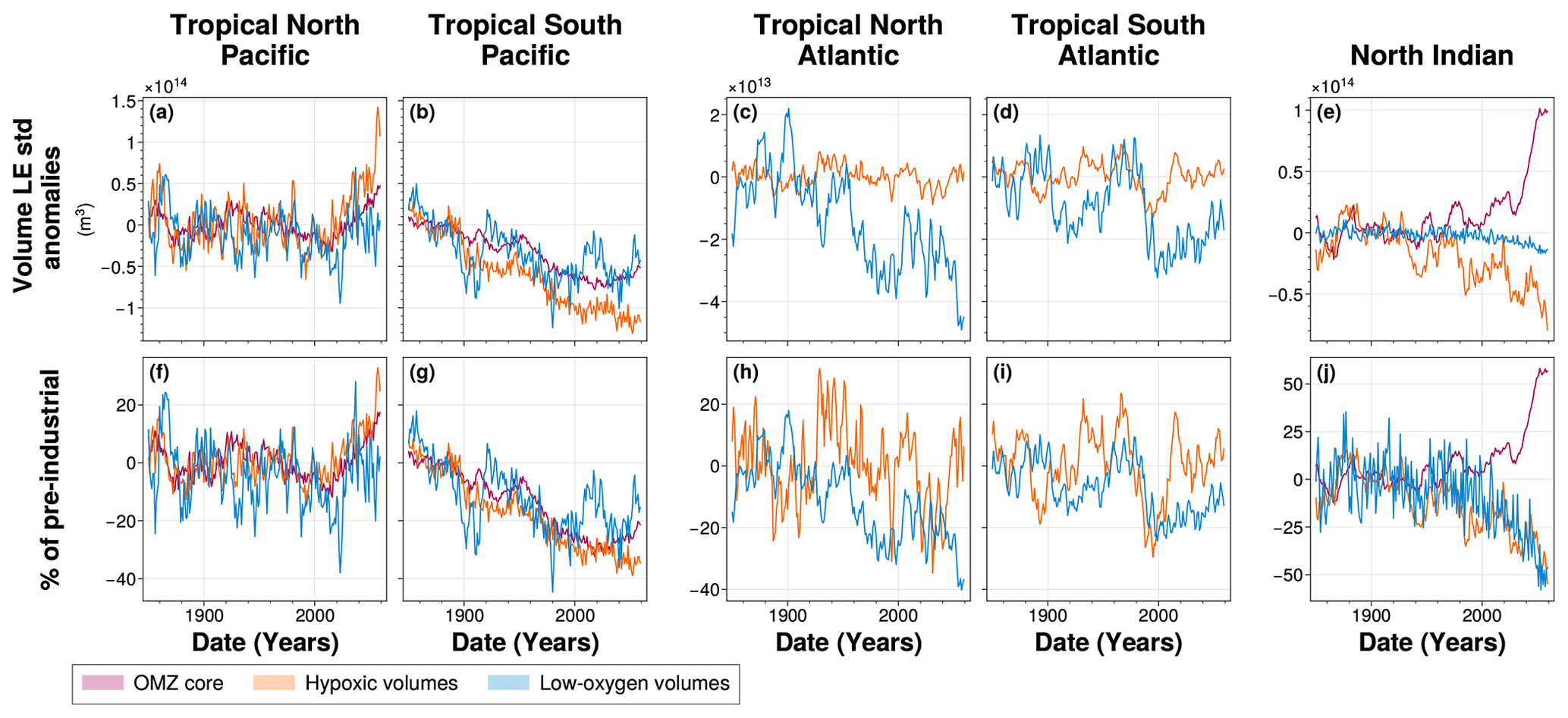
Figure A2 Large Ensemble standard deviation anomalies of 100–1000 m OMZ volumes for (a, f) the tropical North Pacific, (b, g) the tropical South Pacific, (c, h) the tropical North Atlantic, (d, i) the tropical South Atlantic and (e, j) the North Indian ocean. In all panels, colours represent the [O₂] threshold used to define OMZ volumes: (purple) OMZ cores, (orange) hypoxic volumes and (blue) low-oxygen volumes. The Large Ensemble standard deviation anomalies are calculated relative to pre-industrial period (1850–1900) for the (a–e) OMZ volumes and (f–j) percentage of pre-industrial mean volume.

A4 Time of emergence for each grid cell

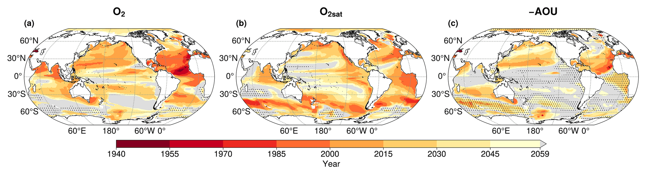
Figure A3 Time of emergence in IPSL-CM6A-LR for the 100–1000 m mean concentration of (a) dissolved oxygen, (b) oxygen saturation and (c) the opposite of the apparent oxygen utilisation. Grey regions indicate area where no emergence of the anthropogenic signal occurs by the end of the simulation in 2059. Dashed areas represent regions where (a) O₂, (b) O_2sat and (c) −AOU increase under the SSP2-4.5 scenario (2014–2059).

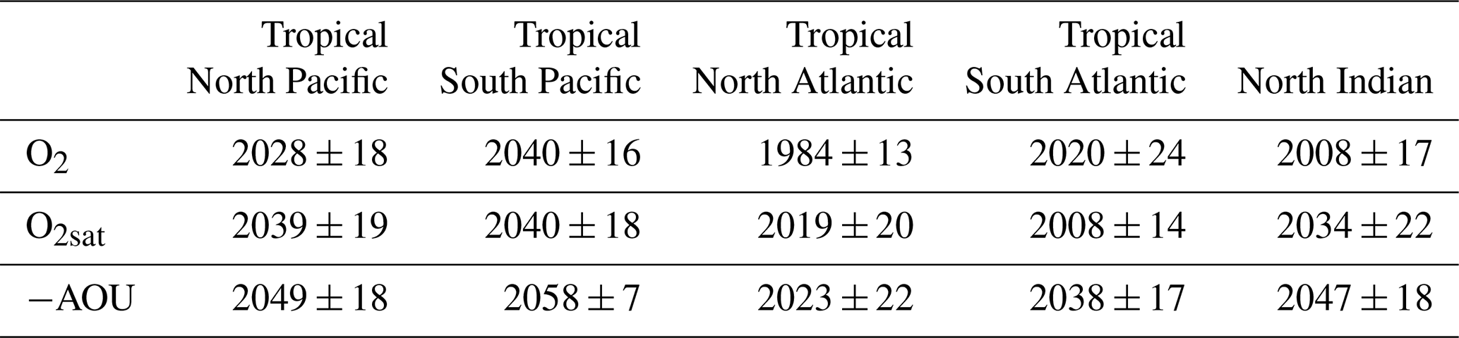
Table A2 Average time of emergence of 100–1000 m spatial mean concentration anomalies for the Large Ensemble mean in each OMZ box. Uncertainty is define as the spatial standard deviation of time of emergence across each OMZ spatial box.

A5 Age since surface contact evaluation

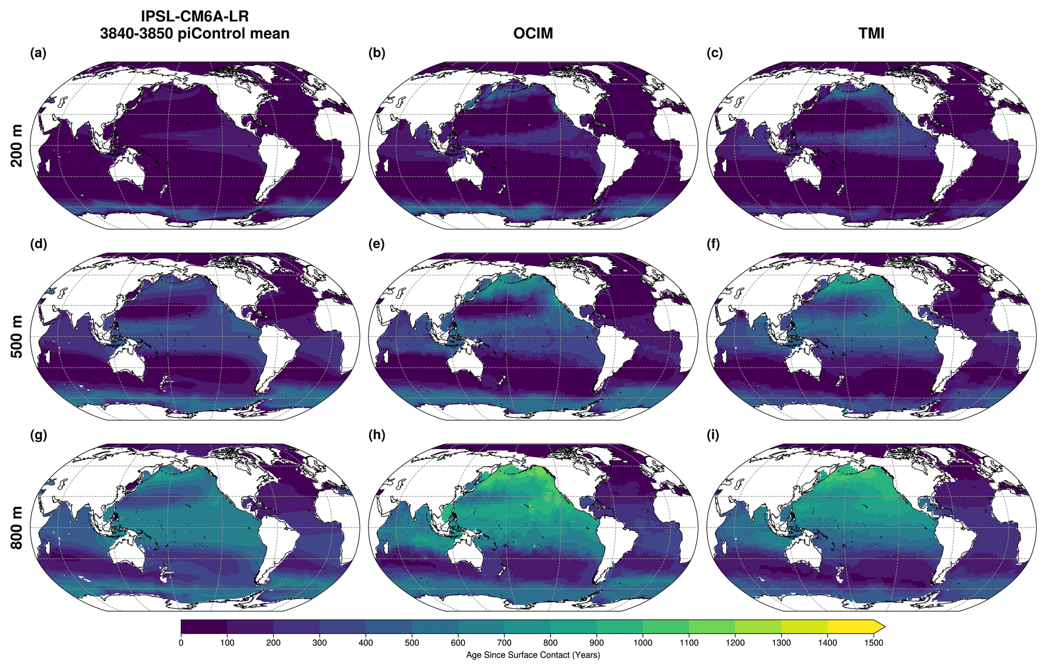
Figure A4 Mean Age Since Surface Contact at (a–c) 200, (d–f) 500 and (g–i) 800 m depth for (a, d, g) the 3840–3850 IPSL-CM6A-LR piControl, (b, e, h) OCIM steady-state (Millet et al., 2025) and (f, i, g) TMI steady-state (Millet et al., 2025).

A6 Sensitivity of time of emergence

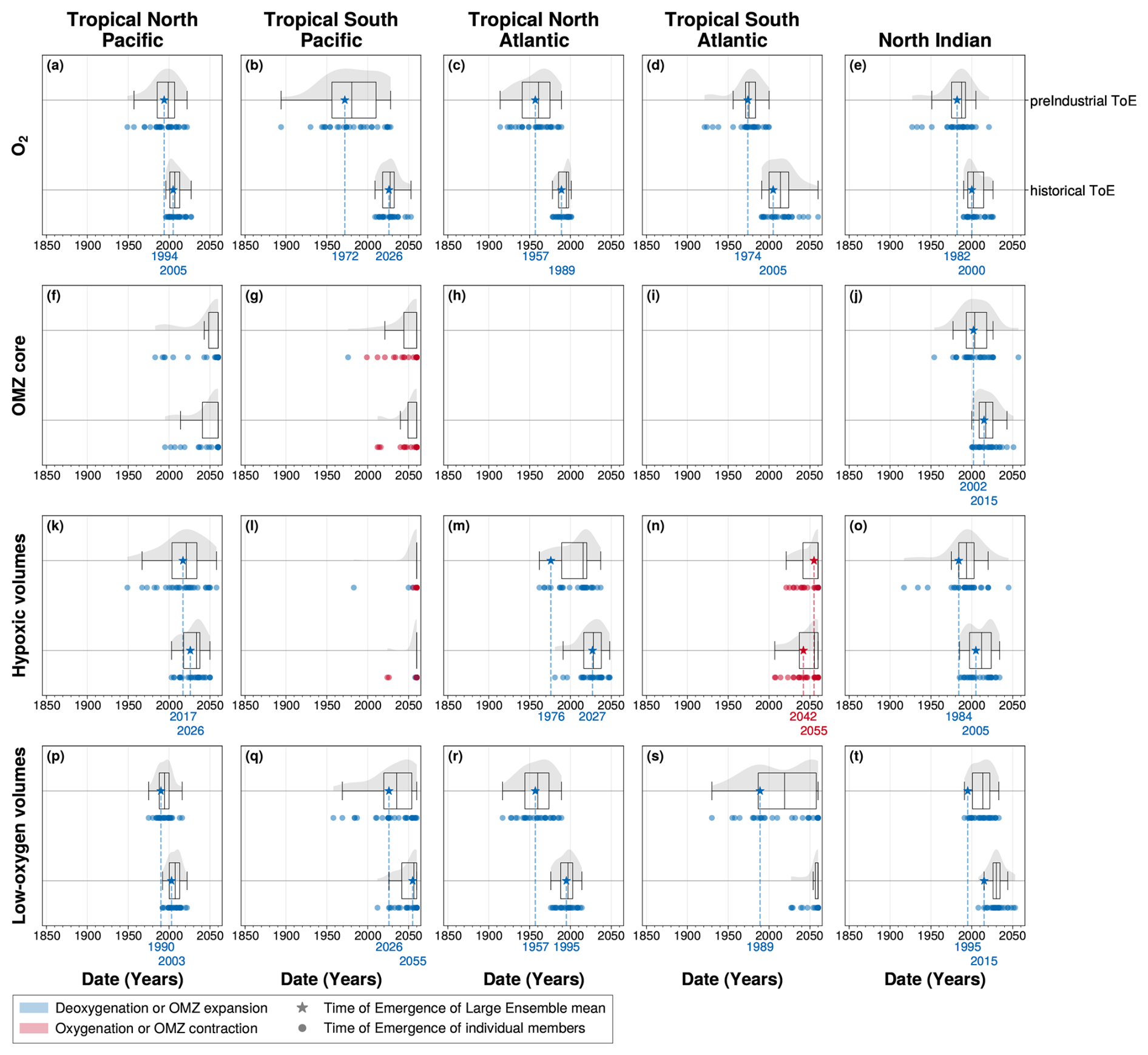
Figure A5 Time of emergence of (panels’ first line) pre-industrial (1850–1900) versus (panels’ second line) historical (1960–1970) anomalies in (a, f, k, p) the tropical North Pacific, (b, g, l, q) the tropical South Pacific, (c, h, m, r) the tropical North Atlantic, (d, i, n, s) the tropical South Atlantic and (e, j, o, t) the North Indian ocean. Times of emergence are computed for 100–1000 m (a–e) spatial mean concentration anomalies of O₂ and OMZ volume anomalies for (f–j) OMZ core, (k–o) hypoxic volumes and (p–t) low-oxygen volumes. In all panels, the box plots illustrate the dispersion of the time of emergence around the median across the IPSL Large Ensemble, while the violin plots illustrate the distribution of the time of emergence within the IPSL Large Ensemble. The star symbol represents the time of emergence for the Large Ensemble mean, defined as the last time at which it exceeds twice the Large Ensemble standard deviation. The dots represent the time of emergence for individual ensemble members signal, defined as the last time at which each member exceeds twice the Large Ensemble standard deviation. Their colours indicate the sign of their trend at the emergence: blue for deoxygenation or OMZ expansion, and red for oxygenation or OMZ contraction.

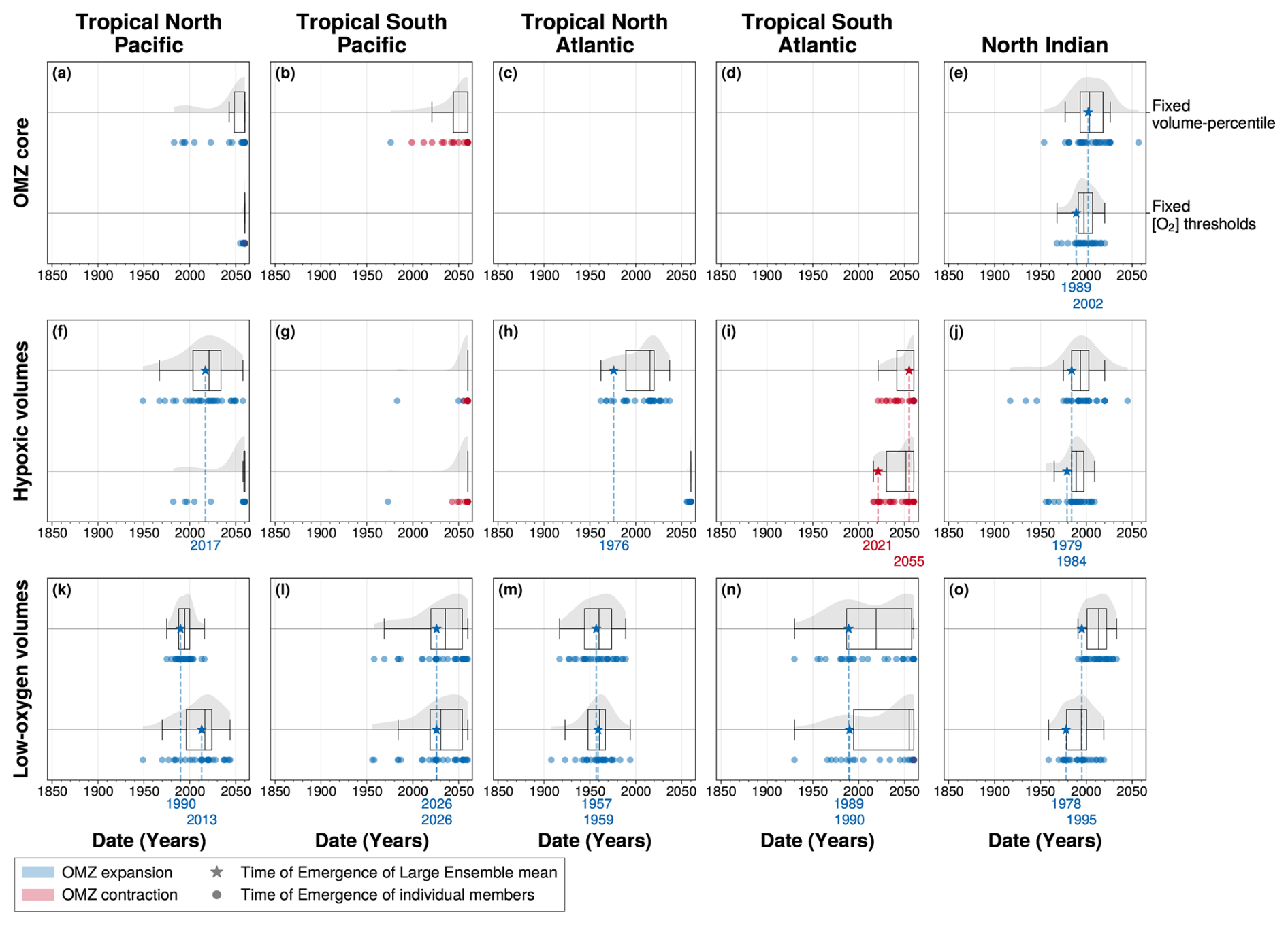
Figure A6 Time of emergence of OMZ volumes defined (panels’ first line) in the ventilation-space with fixed volume-percentile versus (panels’ second line) in the geographic-space with fixed dissolved oxygen concentration thresholds for (a, f, k) the tropical North Pacific, (b, g, l) the tropical South Pacific, (c, h, m) the tropical North Atlantic, (d, i, n) the tropical South Atlantic and (e, j, o) the North Indian ocean. Times of emergence are computed for 100–1000 m OMZ volume pre-industrial (1850–1900) anomalies for (a–e) OMZ core, (f–j) hypoxic volumes and (k–o) low-oxygen volumes. In all panels, the box plots illustrate the dispersion of the time of emergence around the median across the IPSL Large Ensemble, while the violin plots illustrate the distribution of the time of emergence within the IPSL Large Ensemble. The star symbol represents the time of emergence for the Large Ensemble mean, defined as the last time at which it exceeds twice the Large Ensemble standard deviation. The dots represent the time of emergence for individual ensemble members signal, defined as the last time at which each member exceeds twice the Large Ensemble standard deviation. Their colours indicate the sign of their trend at the emergence: blue for deoxygenation or OMZ expansion, and red for oxygenation or OMZ contraction.

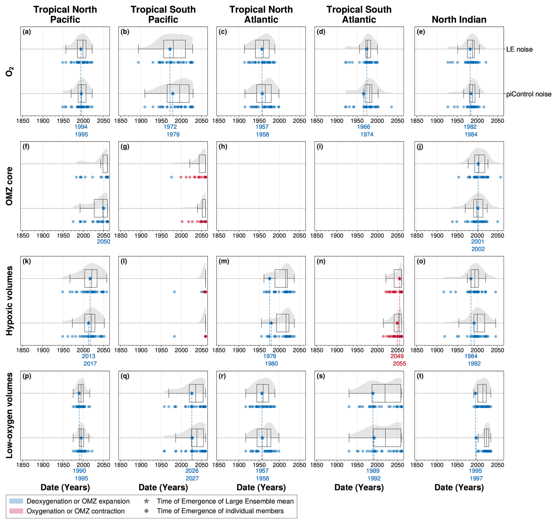
Figure A7 Time of emergence using for noise: (panels' first line) Large Ensemble standard deviation versus (panels' second line) piControl standard deviation. Times of emergence are computed, in (a, f, k, p) the tropical North Pacific, (b, g, l, q) the tropical South Pacific, (c, h, m, r) the tropical North Atlantic, (d, i, n, s) the tropical South Atlantic and (e, j, o, t) the North Indian ocean, between 100–1000 m, for (a–e) spatial mean concentration anomalies of O₂ and OMZ volume anomalies for (f–j) OMZ core, (k–o) hypoxic volumes and (p–t) low-oxygen volumes. In all panels, the box plots illustrate the dispersion of the time of emergence around the median across the IPSL Large Ensemble, while the violin plots illustrate the distribution of the time of emergence within the IPSL Large Ensemble. The star symbol represents the time of emergence for the Large Ensemble mean, defined as the last time at which it exceeds twice the noise. The dots represent the time of emergence for individual ensemble members signal, defined as the last time at which each member exceeds twice the noise. Their colours indicate the sign of their trend at the emergence: blue for deoxygenation or OMZ expansion, and red for oxygenation or OMZ contraction.