Forecasting seasonal global sea surface chlorophyll a with a lightweight data-driven approach

Marine chlorophyll a concentration is a key indicator of ecosystem health, and accurate seasonal forecasting has important applications for fisheries management, harmful algal bloom detection, and climate studies. Traditional approaches rely on computationally intensive numerical biogeochemical models that require extensive domain expertise and parameterization.

We propose a data-driven, resource-efficient alternative: a neural architecture based on the U-Net that reconstructs surface, near-global chlorophyll a based on four physical predictors. The model learns to emulate satellite-like chlorophyll a from mixed layer depth, sea surface height, salinity, and temperature, all of which are known to influence phytoplankton distribution and nutrient availability. By leveraging publicly available seasonal forecasts of these variables, we can generate six-month of chlorophyll a predictions in a matter of minutes with a single GPU.

We trained the model using the GLORYS12 reanalysis as input physics and GlobColour merged chlorophyll a observations as reference. When applied to seasonal forecasting by using SEAS5 ensemble forecasts as input as opposed to the reanalysis, the model maintains high skill globally and remains stable across the six-month forecast horizon. Regional analysis shows that the model accurately captures seasonal dynamics and bloom timings across diverse regimes, with performance comparable to or exceeding that of a state-of-the-art numerical biogeochemical model, while requiring orders of magnitude less computational resources.

This approach demonstrates that high-performing, seasonal chlorophyll a forecasting can be achieved through a resource-efficient, observation-driven framework, offering a practical alternative for operational applications where computational constraints limit the use of full biogeochemical models.

1 Introduction

Like many other natural systems, marine biogeochemical cycles are vulnerable to the effects of climate change (Bopp et al., 2013; Achterberg, 2014). Stressors such as rising temperatures (Polovina et al., 2011), ocean acidification (Orr et al., 2005), and changes in nutrient availability (Achterberg, 2014; Schneider et al., 2008) are already affecting the oceans, and these impacts are expected to intensify in the coming years.

These changes can have cascading effects on marine ecosystems, causing alterations in species distribution and biodiversity, impacting primary production, and posing risks to food security. An important indicator of changes in the health of aquatic ecosystems is chlorophyll a (chl a) concentration. This photosynthetic pigment can be used to estimate phytoplankton biomass and productivity, and it has the additional advantage of being observable from space (Groom et al., 2019), which allows for its large-scale monitoring.

Accurate seasonal chl a forecasting, even if limited to the surface level, can have a variety of important applications. It can help estimate food availability for higher trophic levels, with implications for fisheries management and biodiversity conservation (Park et al., 2019b). Additionally, it enables the early detection of harmful algal blooms, allowing for timely warnings to mitigate their impacts on human health and coastal economies (Lin et al., 2021; Wang et al., 2018). Chl a forecasting also serves as a valuable indicator of upwelling events, which influence nutrient availability and primary production. These processes, in turn, have effects on the carbon cycle and the broader climate system (Bopp et al., 2013; Achterberg, 2014; Rousseaux et al., 2021; Park et al., 2019b).

Traditionally, biogeochemical forecasting has been done using numerical models, which are based on differential equations that model nutrient and carbon cycles (Aumont et al., 2015; Fennel et al., 2022; Berardi, 2020; Gehlen et al., 2015). While some of these models have successfully been used for seasonal chl a forecasting (Rousseaux et al., 2021; Park et al., 2019b), they can be very computationally prohibitive, and they require extensive knowledge of the systems they represent. Incorrect parametrization can lead to systematic biases and uncertainties, and these errors can propagate throughout the model, limiting its capabilities (Fennel et al., 2022; Berardi, 2020; Gehlen et al., 2015).

Machine learning offers the possibility of making use of the growing number of geospatial data for this purpose. While its use in marine biogeochemical modeling is not as widespread as in meteorology, its adoption is steadily growing (Sadaiappan et al., 2023). In the case of chl a, it has been used to enhance remote sensing datasets by filling observational gaps and correcting biases caused by sensor limitations or cloud cover (Keiner, 1999; Hu et al., 2021; Kolluru and Tiwari, 2022; Park et al., 2019a; Cao et al., 2020). Martinez et al. (2020) reconstructed historical chl a patterns from surface oceanic and atmospheric predictors, demonstrating that this approach is able to capture decadal and longer trends of past periods, while Roussillon et al. (2023) further expanded on this work, highlighting the different regional modes of variability. Machine learning has also been applied to short-term chl a forecasting, primarily at regional scales. Park et al. (2015) proposed a support vector machine for forecasts within freshwater and estuarine reservoirs, while Wenxiang et al. (2022) used a neural network to generate forecasts in the Xiamen Bay. Additional examples include Chen et al. (2024), who generated forecasts for freshwater lakes, and Ly et al. (2021), who focused on the Han River. Zhu et al. (2023) and Ying et al. (2023) applied data-driven methods for forecasting in coastal waters. Nonetheless, to our knowledge, most existing efforts focus on regional-scale forecasts spanning only a few days.

Many of these studies demonstrate the feasibility of reconstructing chl a using physical data (Martinez et al., 2020; Roussillon et al., 2023; Chen et al., 2024; Sauzède et al., 2017). Based on this, we propose a machine learning-driven methodology to predict six-months of global, surface-level chl a by using forecasts for the same time period of four oceanic variables: mixed layer depth (MLD), sea surface temperature (SST), sea surface salinity (SSS), and sea surface height (SSH). These variables are selected due to their influence on nutrient and oxygen availability, as well as phytoplankton distribution, making them effective predictors of chl a (Browning and Moore, 2023; Palacios et al., 2013; Fernandez-Gonzalez et al., 2022; Xu et al., 2022; Barone et al., 2019; Uz et al., 2001; Chenillat et al., 2021). They also offer practical advantages: they are readily available from ocean reanalyses, and it is possible to obtain their seasonal forecasts.

The goal of this work is to demonstrate that we can not only estimate chl a from these four variables, but that by using publicly available forecasts of these as input, we are able to generate an ensemble of accurate chl a predictions for six months into the future. Our approach operates at a spatial resolution of approximately 25 km ($\mathrm{1}/\mathrm{4}$°) and two different temporal resolutions: 5 d (as a proof-of-concept of performance at higher temporal resolution) and monthly (to match the available physics forecasts used as input).

2 Proposed Methodology

The predictive task consists of reconstructing the chl a distribution over a six-month horizon using forecasts of four physical predictors. Given the intended practical utility of these predictions in operational settings, our primary objective was to develop a solution that is computationally efficient, operationally robust, and readily deployable under limited computational resources.

Given that the seasonal cycle of chl a is pronounced, we chose to decompose the forecast problem by calendar month rather than addressing it with a single, more complex model. We therefore implemented a month-dependent strategy based on twelve lightweight neural networks, one for each initialization month of the forecast. The training period spans January 1998 to May 2017. Each network was trained on time series of six consecutive months beginning at its initialization: for example, the January network used January–June data from 1998–2016, while the December network used sequences from December to May (1998–2017). Figure 1 provides an overview of the methodology.

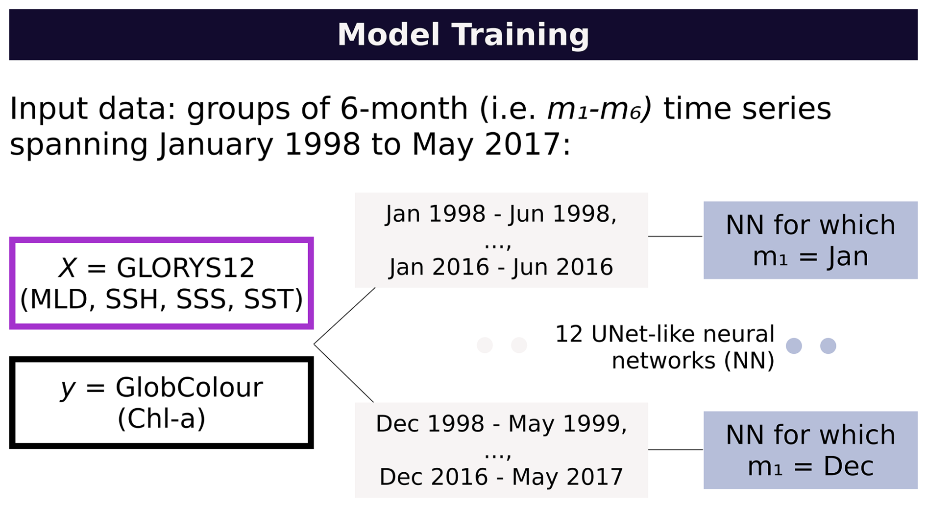
Figure 1 Overview of the methodology: Twelve month-specific neural networks are trained on six-month time series spanning 1998–2017, each initialized on the starting month of the forecast.

This strategy limits the framework's ability to generalize across initialization months and may reduce capacity to learn universal temporal relationships. Nonetheless, it offers some practical advantages: each network is substantially smaller than a unified model, conditioning on the initialization month reduces representational complexity, and the design mirrors the operational workflow, in which users generate chl a forecasts based on physics predictions available from a specific month of initialization. This approach also allows each model to focus on a narrower distribution of patterns, which can be learned effectively with fewer parameters; thus, we considered this an acceptable trade-off.

Two versions of this workflow were created: one using monthly resolution (to match the available physics forecasts that would be used as input operationally), and another using 5 d averages (i.e. 6 data points per month, to test performance at higher temporal resolution). Both architectures use a spatial resolution of $\mathrm{1}/\mathrm{4}$°, or approximately 25 km.

2.1 Training data

The physics data were provided by the Global Ocean Physics Reanalysis (GLORYS12) (Lellouche et al., 2021; Copernicus Marine Service, Marine Data Store, 2024), and the Global Ocean Color (GlobColour) dataset (Garnesson et al., 2019) was used as the output target. GLORYS12 is a high-resolution reanalysis that provides daily and monthly data on the four predictors (MLD, SST, SSS, SSH), among other variables. It is based on the NEMO (Nucleus for European Modelling of the Ocean) platform and driven at the surface by ECMWF's ERA-Interim and ERA5 meteorological reanalyses. Satellite altimetry, SST, sea ice concentration, and in situ temperature and salinity vertical profiles are assimilated (Lellouche et al., 2021).

The GlobColour dataset provides a combination of gap-filled satellite observations of chl a from multiple remote sensors. Chl a concentrations are derived from reflectance using sensor-specific algorithm coefficients and then merged (Garnesson et al., 2019; Maritorena et al., 2010). Because the availability and quality of remotely sensed chl a degrade at high latitudes due to low solar elevation, persistent cloud cover, and sea-ice, we restrict the domain to a −60 to 80° latitude grid in order to ensure robust training targets.

Within the development dataset (January 1998–May 2017), the years 2001, 2005, 2010 and 2015 were used for validation, while the rest was used for training. The training set was used to fit the model, while the validation set served for hyperparameter optimization and selecting the most effective model architecture. After selecting the final parameters using the training and validation sets, the model is evaluated on an independent test set (2018–2023 for the 5 d model and 2020–2023 for the monthly model).

The physical ocean data were normalized using min-max scaling and the chl a data were log-transformed. Both datasets are available at a daily resolution, and the data were averaged to monthly and 5 d resolutions for training the respective versions of the model. The $\mathrm{1}/\mathrm{12}$° GLORYS12 grid was coarsened using bicubic interpolation to match the observational grid resolution, which was obtained at $\mathrm{1}/\mathrm{4}$°.

2.2 Training objective

The proposed methodology reconstructs a six-month chl a grid ($\widehat{y}$) given a corresponding six-month input grid of four physical variables ($X=\mathit{\{}\text{MLD},\text{SST},\text{SSS},\text{SSH}\mathit{\}}$). As mentioned above, the network operates on log-transformed chl a values, where $p_i=\log \left({\widehat{y}}_i\right)$ denotes the predicted values for the ith grid point, and r_i=log (y_i) denotes the corresponding log-transformed reference point. The training objective is defined as the mean squared error (MSE) between the network output and the reference:

$$\begin{array}{}\text{(1)}& \text{MSE}={\displaystyle \frac{\mathrm{1}}{N}}\sum _{i=\mathrm{1}}^N(r_i-p_i{)}^{\mathrm{2}}\end{array}$$

where N is the total number predicted points in the training batch.

In spite of the log-transformation, initial assessments showed that the model had a tendency to underestimate chl a concentrations, so the standard MSE loss function was modified by adding a small penalty for underestimation. This adjustment was based on empirical testing and was implemented by applying a small weight w whenever the underestimation occurred:

$$\begin{array}{}\text{(2)}& \mathcal{L}={\displaystyle \frac{\mathrm{1}}{N}}\sum _{i=\mathrm{1}}^N\left[\right(r_i-p_i{)}^{\mathrm{2}}+w\cdot [max(\mathrm{0},r_i-p_i\left){]}^{\mathrm{2}}\right]\end{array}$$

where the second term applies an additional penalty $w\cdot (r_i-p_i{)}^{\mathrm{2}}$ when p_i<r_i. While this approach was effective in reducing underestimation, more principled methods could provide a more robust solution.

2.3 Model architecture

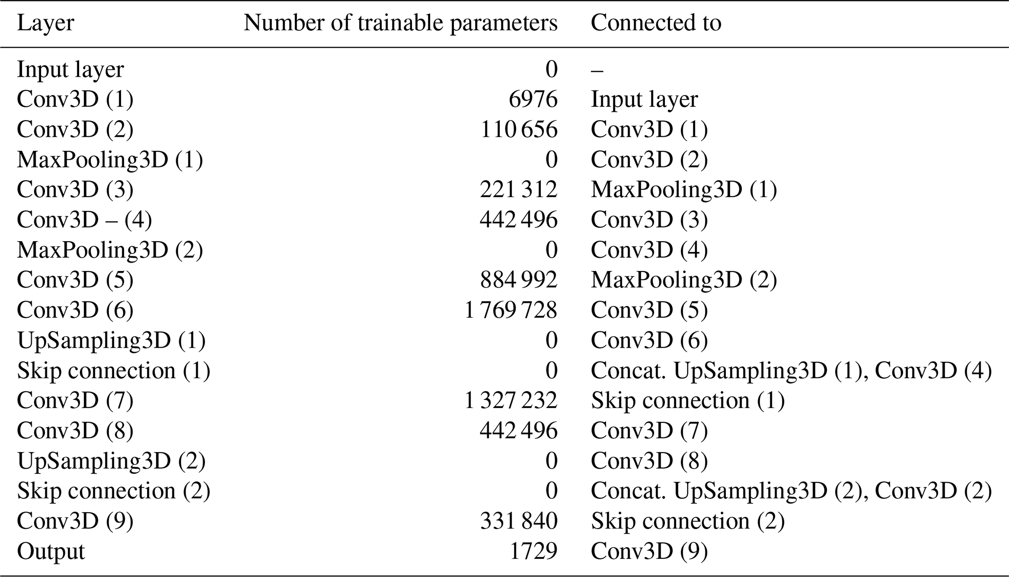
The neural networks are based on the U-Net architecture (Ronneberger et al., 2015), a convolutional neural network with an encoder-decoder structure that has been widely applied to Earth science forecasting tasks due to the grid-based nature of such data (Agrawal et al., 2019; Sønderby et al., 2020; Weyn et al., 2019, 2021). The U-Net's skip connections enable it to combine low-level spatial details with high-level semantic information, allowing reconstruction of both large-scale patterns and fine-scale features simultaneously. Despite advances and increased complexity in more recent architectures, the U-Net's simplicity and efficiency make it an effective and resource-efficient choice for this task. To process both spatial and temporal dimensions simultaneously, we use 3D convolutions (Tran et al., 2015). To balance the additional computational cost of the 3D convolutions, the proposed architecture uses fewer layers and filters than the original U-Net.

The encoder consists of two blocks of convolutional and max-pooling layers, which downsample the input. Two additional convolutional layers refine feature extraction before transitioning to the decoder, which mirrors the encoder and upsamples the data back to the original resolution. Skip connections link matching layers of corresponding size in the encoder and decoder (see Table 1). A rectified linear unit (ReLU) activation function was used throughout the network, except in the output layer, where a Softplus activation function (Dugas et al., 2000) was empirically found to work best. The model architecture is summarized in Table 1.

Table 1 Summary of proposed neural architecture.

All twelve models share a common architecture and hyperparameters (i.e. number and order of layers, number of convolutional filters and kernel size, learning rate, etc.), which were optimized empirically and using random search. The models were trained using the Adam optimizer (Kingma and Ba, 2017) and a learning rate of 0.001 for a maximum of 300 epochs. We used early stopping on the validation loss to prevent overfitting, but no explicit regularization methods were used. We also used transfer learning, where the training process of a model can be initialized with the pre-trained weights of another, to further optimize computational cost. The models were trained on a single GPU (NVIDIA A100, 40 GB).

2.4 Model evaluation and prediction generation

We evaluate our approach by using two distinct setups, each serving a different purpose. First, we perform a preliminary validation at a 5 d resolution using the GLORYS12 reanalysis as input. We generate a set of 5 d predictions covering the 2018–2023 period. This step isolates the model's ability to map physics to chl a when given accurate, observation-constrained physics, and serves to assess performance at a higher temporal resolution. We then validate seasonal forecast generation using 6 month forecasts from the ECMWF SEAS5 system (Johnson et al., 2019) as input. This is performed for the 2020–2023 period at a monthly temporal resolution to align with the available input data. This setup mimics the intended application of the model, where the chl a predictions would rely on predicted physics as opposed to a reanalysis. Both approaches use a spatial resultion of $\mathrm{1}/\mathrm{4}$°. We describe the SEAS5 system in more detail below.

The forecast consists of an ensemble of 51 members, and it uses the IFS (Integrated Forecasting System) cycle 43r1 for the atmosphere, NEMO for the ocean, and LIM2 (Louvain-la-Neuve Sea Ice Model version 2) for sea ice. The system assimilates temperature, salinity, satellite altimetry, and snow cover (Johnson et al., 2019). The forecasts are available free of charge on the Copernicus Climate Data Store at a monthly, one-degree resolution (Copernicus Climate Change Service, Climate Data Store, 2018a, b). A version of higher spatial resolution ($\mathrm{1}/\mathrm{4}$°) of the data was kindly provided by ECMWF, but it is possible to obtain similar results by downscaling with a simple interpolation method.

The SEAS5 forecast exhibits some biases relative to the reanalysis (see Fig. 2), which is expected given their different sources and purposes. To account for this, we computed the difference between the monthly climatologies of both datasets over the training period (1998–2017), then subtracted this mean bias from the SEAS5 data before using it as model input. This offset is computed once, and can be applied to all forecasts, including future ones.

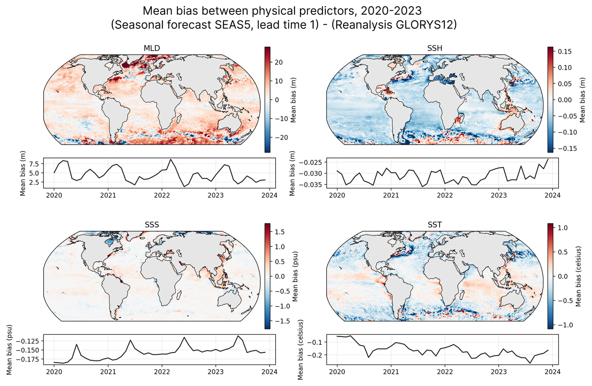
Figure 2 Mean biases between SEAS5 (monthly forecast, one-month lead time) and GLORYS12 for the input variables over the 2020–2023 period. While correction is applied using historical climatological differences (see Methods), this figure is indicative of the systematic differences between the forecast and reanalysis.

We used the first 10 (out of 51) ensemble members from SEAS5 as input for the neural network to generate six-month predictions at a monthly resolution (i.e. matching the available forecast resolution), using forecasts initialized from January 2020 to December2023. To evaluate performance across different lead times (i.e., the number of months after forecast initialization), we constructed six continuous time series by concatenating the corresponding month from each six-month forecast. Specifically, we extracted the first month from each forecast to create a one-month lead time series (January 2020–December 2023), the second month from each forecast for a two-month lead time series (February 2020–January 2024), and so on. This is illustrated in Fig. 3 for clarity. We compute SEAS5-based skill metrics over January 2020–December 2023 (i.e., truncating any lead time series months that extend into 2024).

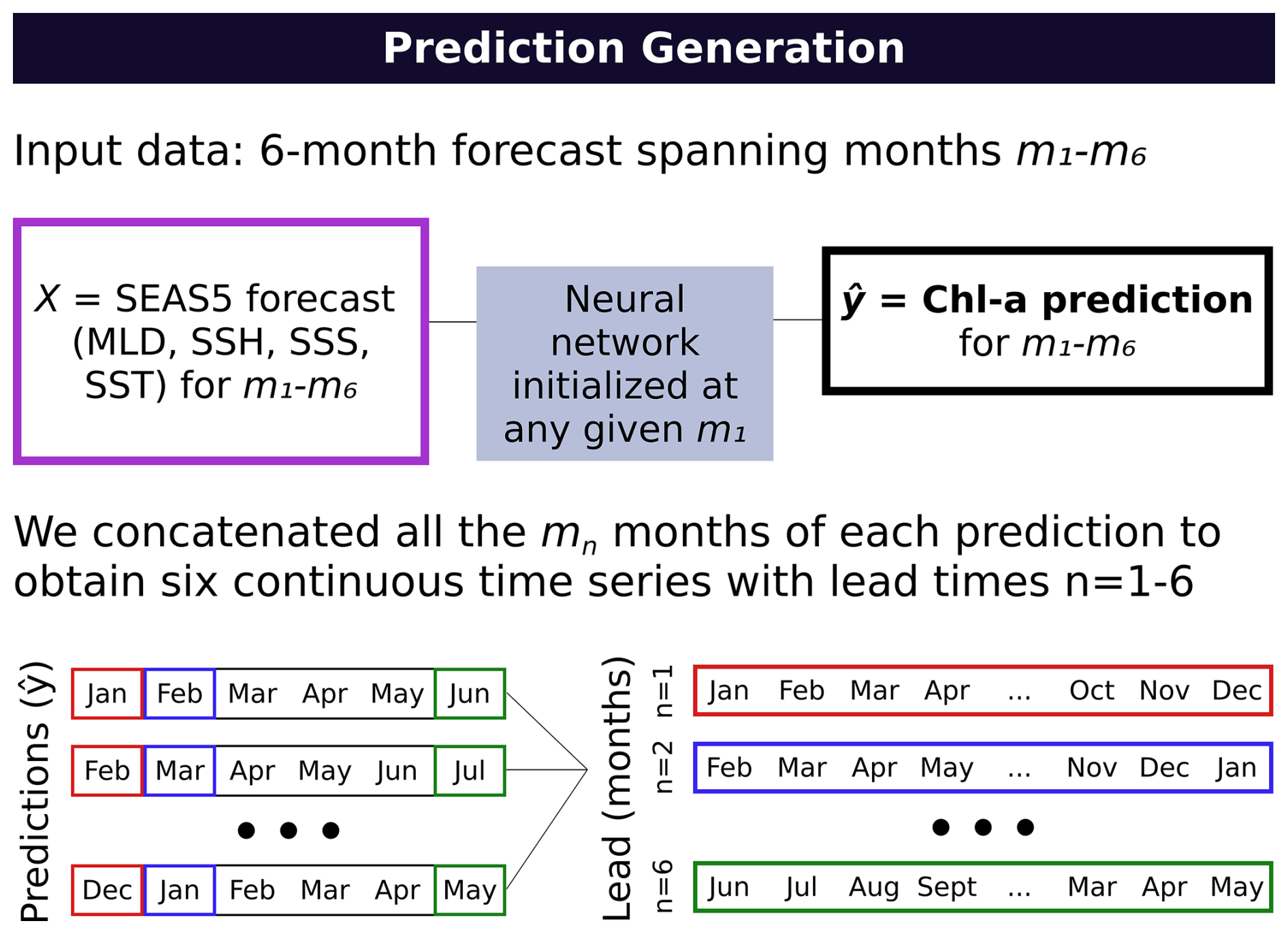
Figure 3 A summary of the prediction generation workflow: We concatenated the nth months from each prediction to generate continuous time series with lead times 1–6 (months).

We analyzed performance by zooming into some open-ocean regions of interest: the North Pacific (170° E–130° W, 25–45° N), Tropical Pacific (170° E–100° W, 10° S–10° N), South Pacific (170–100° W, 35–15° S), North Atlantic (70–20° W, 25–40° N), and Indian Ocean (55–95° E, 25–0° S), which are based on Park et al. (2019b). We also examined model skill in the Equatorial Atlantic (35° W–5° E, 5° S–5° N) and in selected large coastal ecosystems, specifically the California Current (25–45° N, 130–113° W), Humboldt Current (50–5° S, 85–69° W), South China Sea (1–25° N, 105–119° E), Gulf of Mexico (18–30° N, 100–80° W), Benguela Current (35–12° S, 5–20° E), Bay of Bengal (5–25° N, 80–98° E), Celtic-Biscay Shelf (43–55° N, 15° W–0° E), and Northeast Australian Shelf (25–10° S, 140–155° E). These regions are illustrated in Fig. 4.

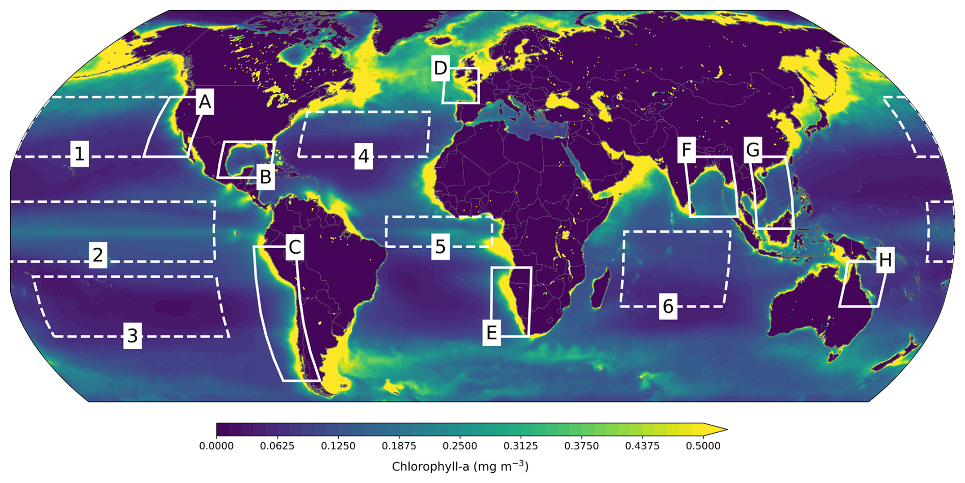
Figure 4 Regions where performance is evaluated. Open-ocean (dashed lines): North (1), Tropical (2) and South Pacific (3), North (4) and Equatorial Atlantic (5), and Indian Ocean (6). Coastal large ecosystems (solid lines): California Current (A), Gulf of Mexico (B), Humboldt Current (C), Celtic-Biscay Shelf (D), Benguela Current (E), Bay of Bengal (F), South China Sea (G), and Northeast Australian Shelf (H).

We evaluated our results against BIO4, a state-of-the-art global biogeochemical product from Mercator Océan International (Copernicus Marine Service, Marine Data Store, 2023). BIO4 is based on the PISCES model (Pelagic Interactions Scheme for Carbon and Ecosystem Studies), the biogeochemical component of the NEMO platform (Lamouroux et al., 2023; Aumont et al., 2015). It simulates global cycles of carbon, oxygen, and key nutrients, includes two functional groups each of phytoplankton and zooplankton, and produces a 3D representation of nearly 30 biogeochemical variables. BIO4 provides both analyses and 10 d forecasts down to 5700 m depth. The model is driven by GLO12, a near-real-time physical reanalysis based on GLORYS12, the training input physics in our study, and it assimilates GlobColour observations on a weekly basis (Lamouroux et al., 2024).

Our evaluation focused on the surface layer of the BIO4 analysis (rather than the forecast) due to differing forecast horizons. We note that BIO4 simulates a wide range of biogeochemical variables and processes beyond surface chl a, while our neural network is specifically optimized for chl a prediction and trained directly on observational data. We therefore use BIO4 as a contextual benchmark rather than a direct point of comparison.

We evaluate model skill primarily using RMSE and Pearson correlation computed on the raw (non-log-transformed) chl a fields. All figures in this manuscript use non-log-transformed chl a. Because different diagnostics emphasize different aspects of performance, we report two complementary RMSE definitions. For the regional time series shown in Figs. 11–14, we first spatially average each field over the region to obtain a region-mean time series, then compute RMSE between the ensemble-mean forecast and the GlobColour reference over 2020–2023 (with RMSE of the BIO4 analysis computed on the same dates). For the regional RMSE summaries (Figs. 10, 16, and 17), we compute RMSE within each region using all valid grid-point samples over 2020–2023 either for a given calendar month (Figs. 16 and 17) or averaged across months (Fig. 10). For anomaly visualizations (Figs. 12 and 14), anomalies are computed relative to a monthly historical climatology based on GlobColour (1998–2017). This provides a stable observation-based baseline while retaining systematic forecast biases.

3 Results

3.1 Model validation with reanalysis physics as input

To validate the neural network architecture and isolate model performance from forecast uncertainties, we first evaluated the model using GLORYS12 reanalysis as input physics. We generated predictions for 2018–2023 at a 5 d temporal resolution. Figure 5 shows that the globally averaged (spatial mean at each time step) time series of the neural network predictions exhibits good visual agreement with the observations. We also included outputs from the BIO4 analysis (dashed lines) for comparison. The neural network captures both the amplitude and phasing of the dominant signal. Although it slightly overshoots seasonal peaks, it represents seasonal lows more accurately than BIO4. This validates the model's ability to learn the relationship between the four physical variables and biological productivity.

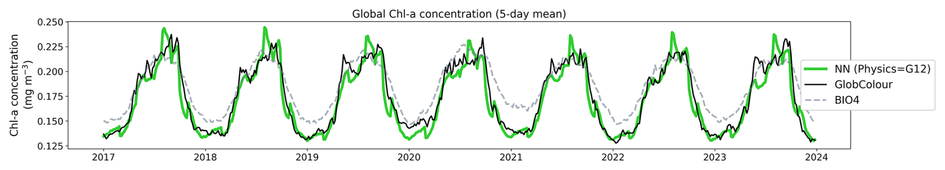
Figure 5 Globally averaged chl a concentration time series from 2018 to 2023. The neural network predictions using GLORYS12 reanalysis as input physics (green line) are compared against GlobColour satellite observations (black line) and outputs from the BIO4 analysis (dashed lines).

To assess spatial skill, Fig. 6 presents a global map of Pearson correlation coefficients (r) computed at each grid point between the predictions and observations. Correlation values were computed for monthly-averaged data over the 2020–2023 period to facilitate comparison with the forecasting results, which have lower temporal resolution and only cover that temporal period. The correlation map shows strong spatial coherence, with positive correlation values across most of the global ocean. Regions of particularly high correlation are found in the Northern oceans, while the Tropical and South Pacific show less skill.

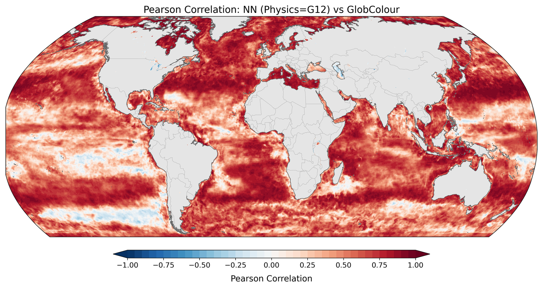
Figure 6 Spatial distribution of Pearson correlation coefficients between the neural network predictions (with GLORYS12 as input physics) and the observations. Correlation values are computed at each grid point for the monthly-averaged data over the 2020–2023 period for better comparison with forecasting results.

3.2 Seasonal forecast performance

We next evaluated the model in a forecasting configuration by using SEAS5 seasonal forecasts as input physics. All results presented below use the monthly model and the SEAS5 ensemble (10 of 51 members) as input. We note here that the chl a reconstruction model is deterministic, and the ensemble spread arises solely from the SEAS5 physical ensemble.

We generated 6 month forecasts at monthly resolution for 2020–2023. Figure 7 displays the globally averaged time series for forecasts initialized in March, June, September and December, with individual ensemble member trajectories shown as thin lines and initializations indicated by colored markers. The ensemble forecasts are visually consistent with the observations, with individual member trajectories continuing to follow the observed chl a concentrations throughout the 6 month forecast horizon, indicating little skill degradation with increasing lead time.

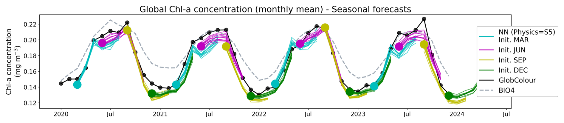
Figure 7 Globally averaged chl a concentration time series from 2020 to 2023 reconstructed from the seasonal forecasts. The forecasts were initialized in March (cyan), June (magenta), September (yellow), and December (green), and the individual member reconstructions are shown as thin lines. Initialization (lead time 1) months are indicated by large colored markers. GlobColour observations are shown in black and BIO4 outputs are shown in dashed lines.

Figure 8 illustrates spatial skill using the Pearson correlation coefficient between predictions and observations over the 2020–2023 period, shown for one and six-month lead times. Correlations remain spatially coherent but a small reduction in skill is observed relative to the GLORYS12 driven predictions (Fig. 6). This slight decrease is expected from the transition to forecast inputs, since they can introduce a distributional shift relative to the training data (Fig. 2) even after the bias correction applied to SEAS5 (see Methods). The discrepancies occur mostly in the tropical and southern Pacific, the Indian Ocean, and plume-influenced regions near Brazil and to the south of the Gulf of Guinea. We also note that the southern and tropical Pacific exhibit relatively modest skill even in the GLORYS12 validation, suggesting that our particular modeling framework might be suboptimal for these regions, irrespective of the physics being used as input. Nonetheless, skill remains high in the subtropical gyre regions, where correlations are strong and spatially consistent. Additionally, the large-scale correlation patterns show little degradation from lead time one to six-months, indicating that the spatial skill of the predictions is relatively stable over the forecast horizon.

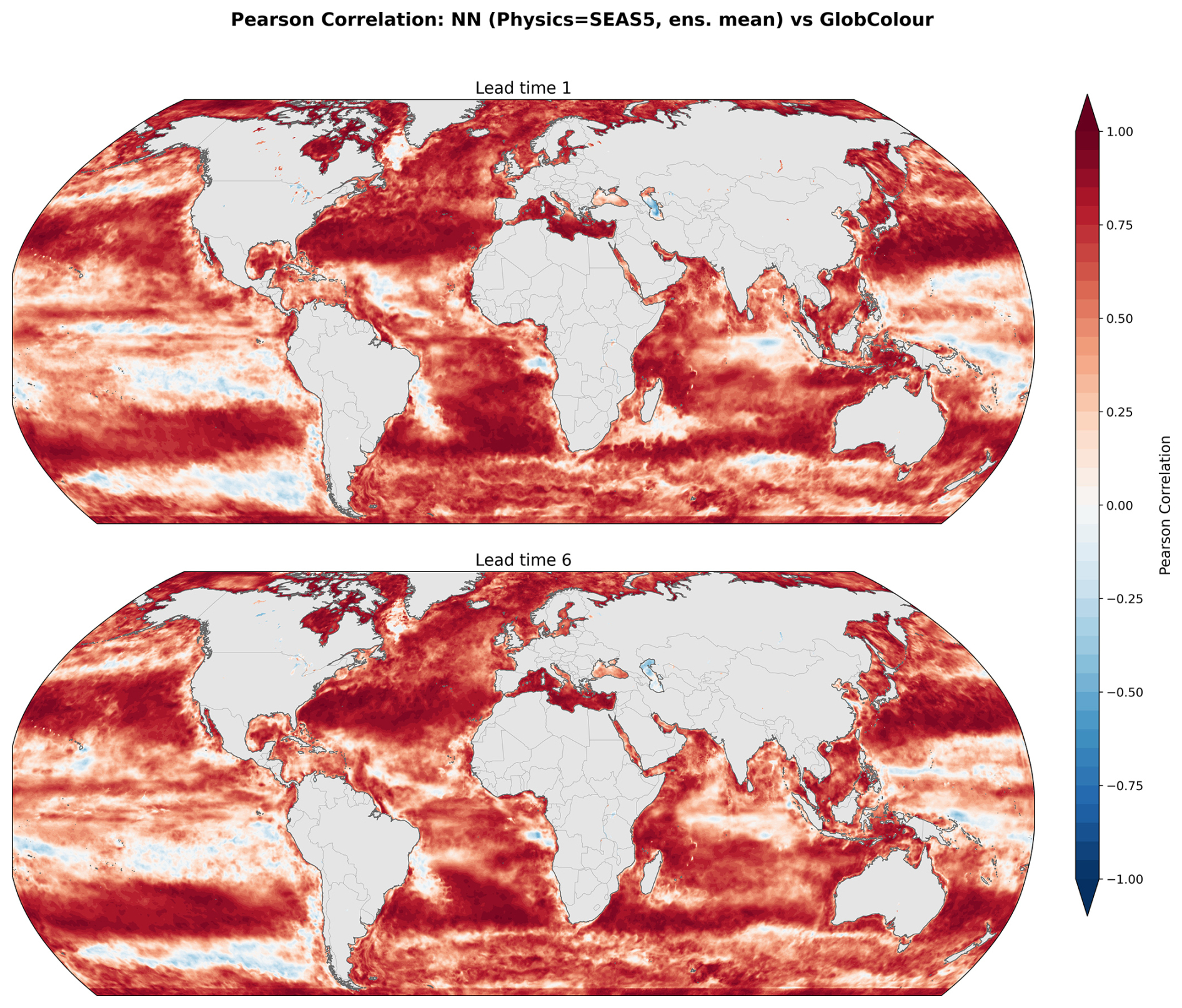
Figure 8 Spatial distribution of Pearson correlation coefficients for seasonal forecasts (SEAS5 used as input physics) at one and six-month lead times over 2020–2023. The ensemble-mean forecast is compared against GlobColour observations.

Figure 9 summarizes skill within each region from Fig. 4 using Pearson's r computed against the GlobColour reference. For each region (and lead time), r is computed using all valid grid-point pairs in the ensemble-mean forecast within the region for each calendar month (pooling 2020–2023), and then averaged across months. In the open-ocean regions (Fig. 9, top), correlations are generally higher than 0.7. The neural-network forecasts outperform BIO4 in the northern basins, consistent with the strong performance visible in Fig. 8. They also outperform BIO4 in the Equatorial Atlantic, although skill there remains weak for the neural model too, as shown in Fig. 8. Performance is lower than BIO4 in the tropics and in the South Pacific and Indian Ocean, again consistent with the poor performance visible in Fig. 8.

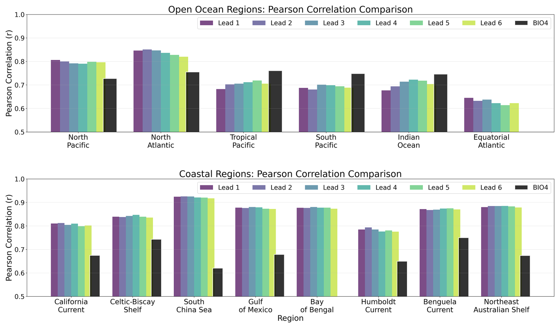
Figure 9 Comparative overview of Pearson correlation coefficients for seasonal forecasts at lead times 1–6 (months) over 2020–2023 for different regions. Note that the y axis is cut off at r=0.5.

In the coastal regions (Fig. 9, bottom), correlations are often higher (typically r≳0.8) and exceed BIO4 in all analysed regions, which is notable given the lack of explicit biogeochemical inputs and the challenges of coastal dynamics, although Fig. 8 shows that this performance is far from uniform. Across regions, correlations show limited sensitivity to lead time, with little degradation from lead times one to six-months.

Figure 10 summarizes regional RMSE for the chl a fields. For each region and lead time, similarly to r, the RMSE is computed over all valid grid cells of the ensemble-mean for each calendar month, and then averaged to obtain a single regional RMSE per lead time. The neural model exhibits lower RMSE than BIO4 across all regions considered, including regions where its correlation is lower (see Fig. 9). This indicates that, in those regions, the neural model is closer to the reference in absolute value even if it might be missing specific patterns (such as spatial shifts in mesoscale features), which can penalize correlation more strongly than RMSE. This is consistent with Fig. 15, where the neural predictions generally match the mean level and broad seasonal evolution of GlobColour but can show small timing/position offsets in bloom development. Conversely, although correlations are often higher in coastal regions, RMSE is also higher on average (note the larger y axis scale), consistent with the larger variability and dynamic range of coastal chl a.

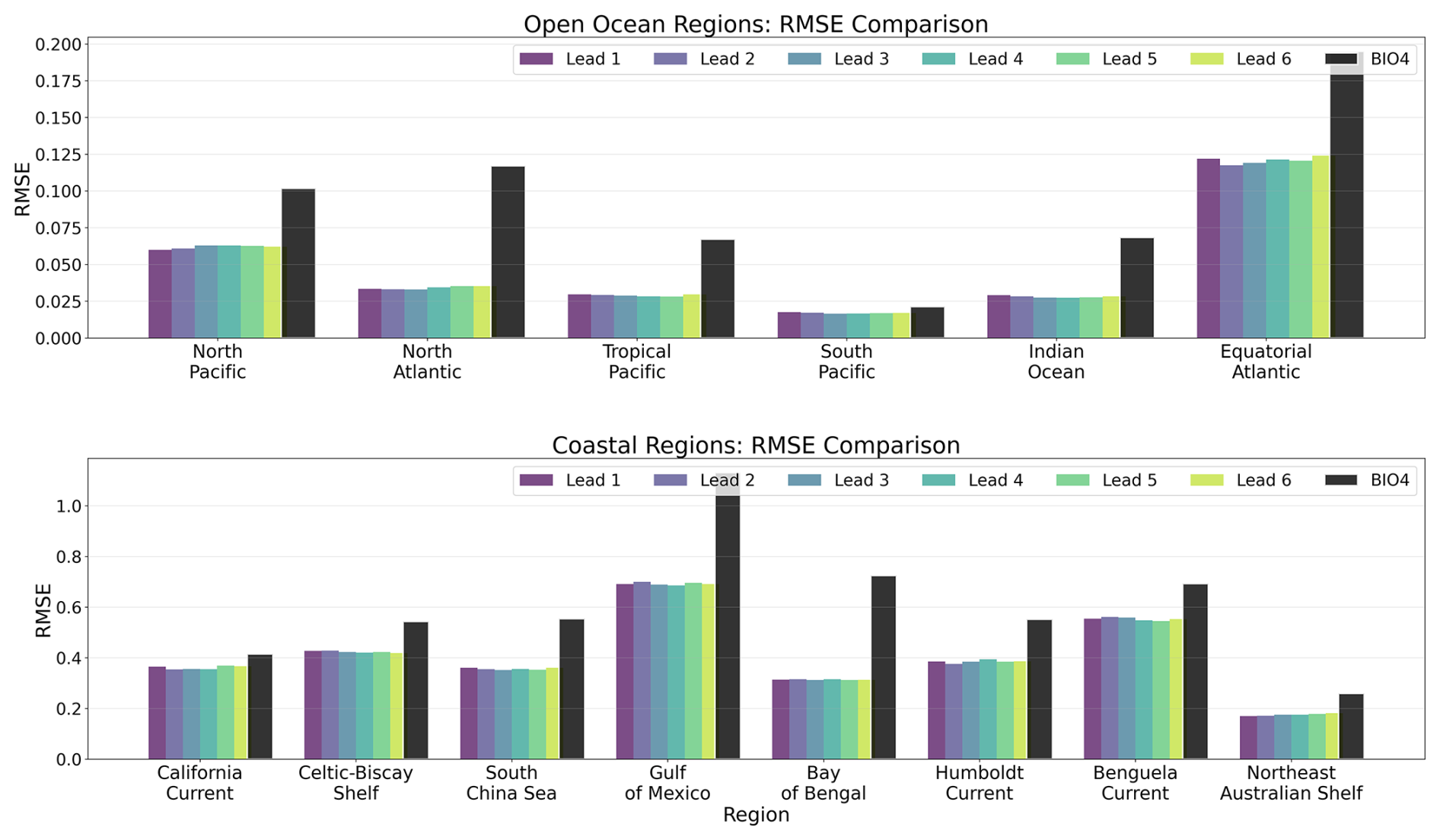
Figure 10 Comparative overview of RMSE for seasonal forecasts at lead times 1–6 (months) over 2020–2023 for different regions, compared to the BIO4 analysis.

3.3 Further examining regional performance

Having assessed global-average skill, we now examine performance in the specific regions highlighted in Fig. 4 more in detail.

Figures 11 and 13 show regional time series for forecasts, this time initialized in January, April, July, and October. For each region, we compare the neural network predictions, the GlobColour reference observations, and the BIO4 analysis. Figures 12 and 14 show the corresponding anomalies, computed by subtracting a monthly GlobColour climatology (computed over 1998–2017) from each region to assess the ability to predict deviations from the seasonal cycle. We report the RMSE for each regional (and corresponding anomaly) time series, computed between the ensemble-mean forecast and the regional GlobColour time series over 2020–2023 (with BIO4 RMSE computed on the same dates). These time-series RMSE values quantify errors in the integrated regional signal after spatial averaging and thus complement the gridpoint-based RMSE reported in Fig. 10.

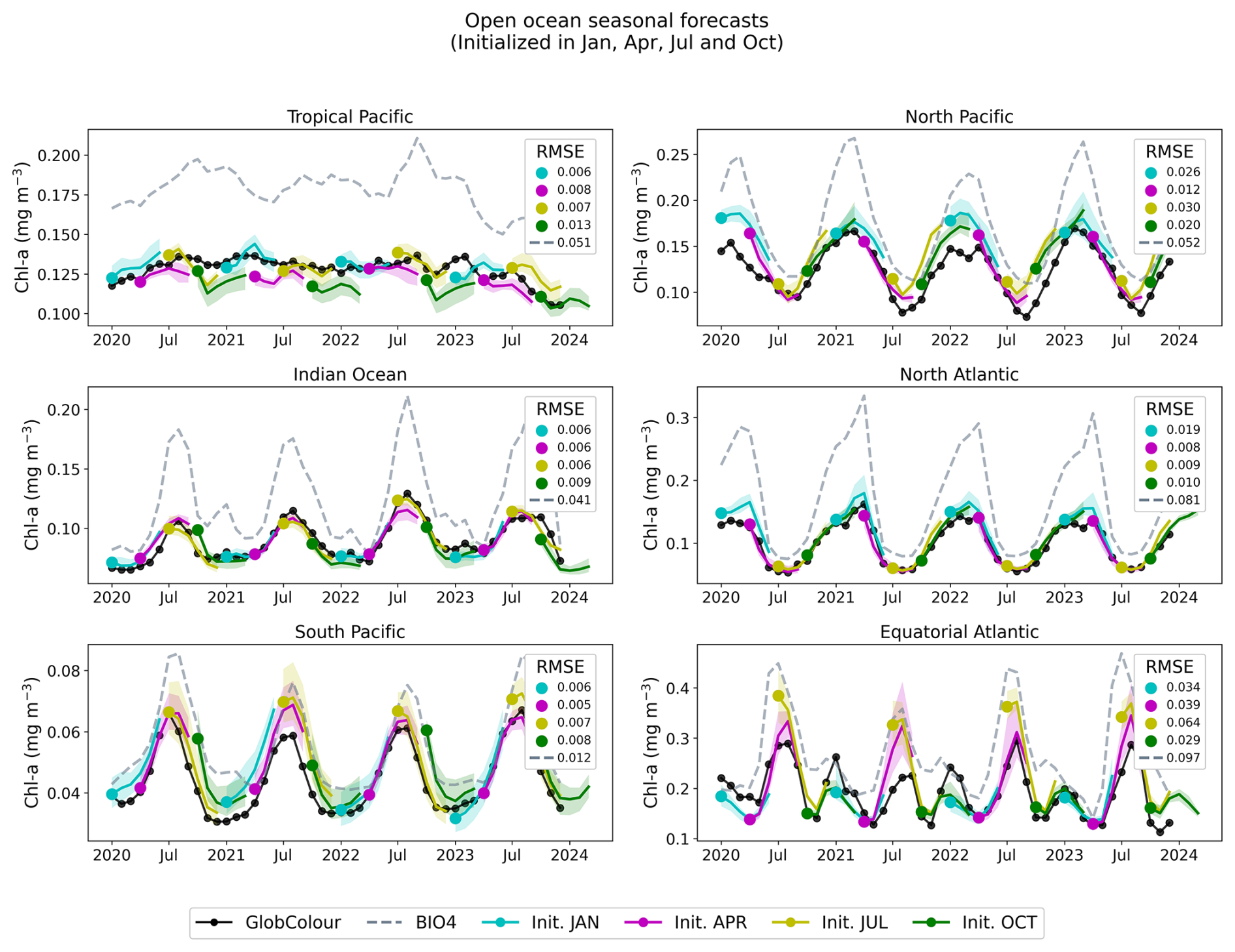
Figure 11 Regional, open-ocean forecasts. The solid black line represents the average GlobColour reference value for each region, while the dashed lines indicate the corresponding BIO4 output. The solid colored lines represent the ensemble average for the neural network-predicted values initialized on January, April, July, and October, while the shading represents the ensemble standard deviation. We report RMSE (computed after spatial averaging) for BIO4 and each group of predictions.

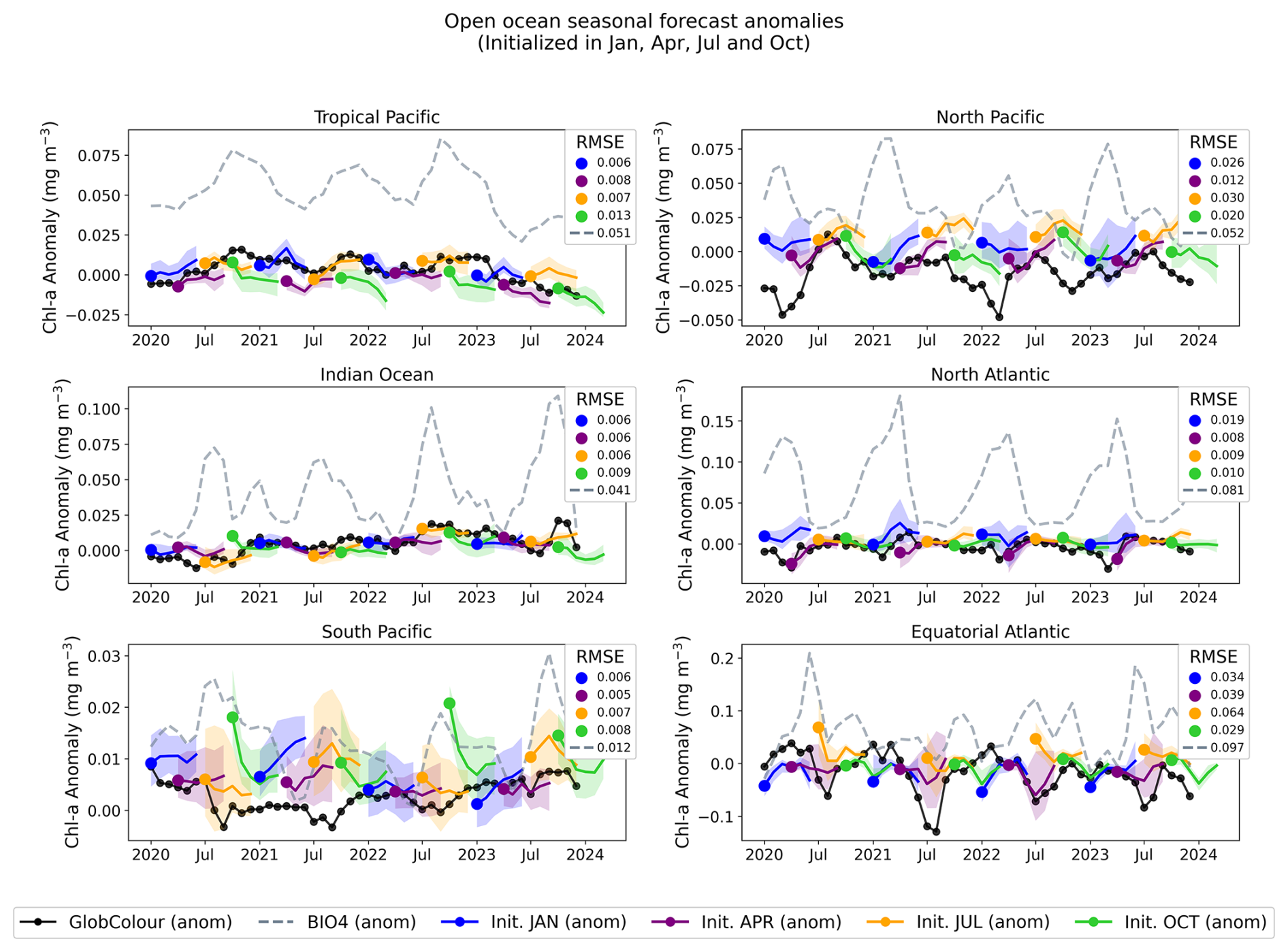
Figure 12 Regional, open-ocean forecasted anomalies. Anomalies are computed by subtracting the monthly GlobColour climatology (seasonal cycle, computed over 1998–2017) from each region-mean time series. The solid black line shows the GlobColour anomaly, dashed lines show the corresponding BIO4 anomaly, and solid colored lines show the ensemble-mean neural-network anomaly forecasts initialized in January, April, July, and October; shading indicates the ensemble standard deviation.

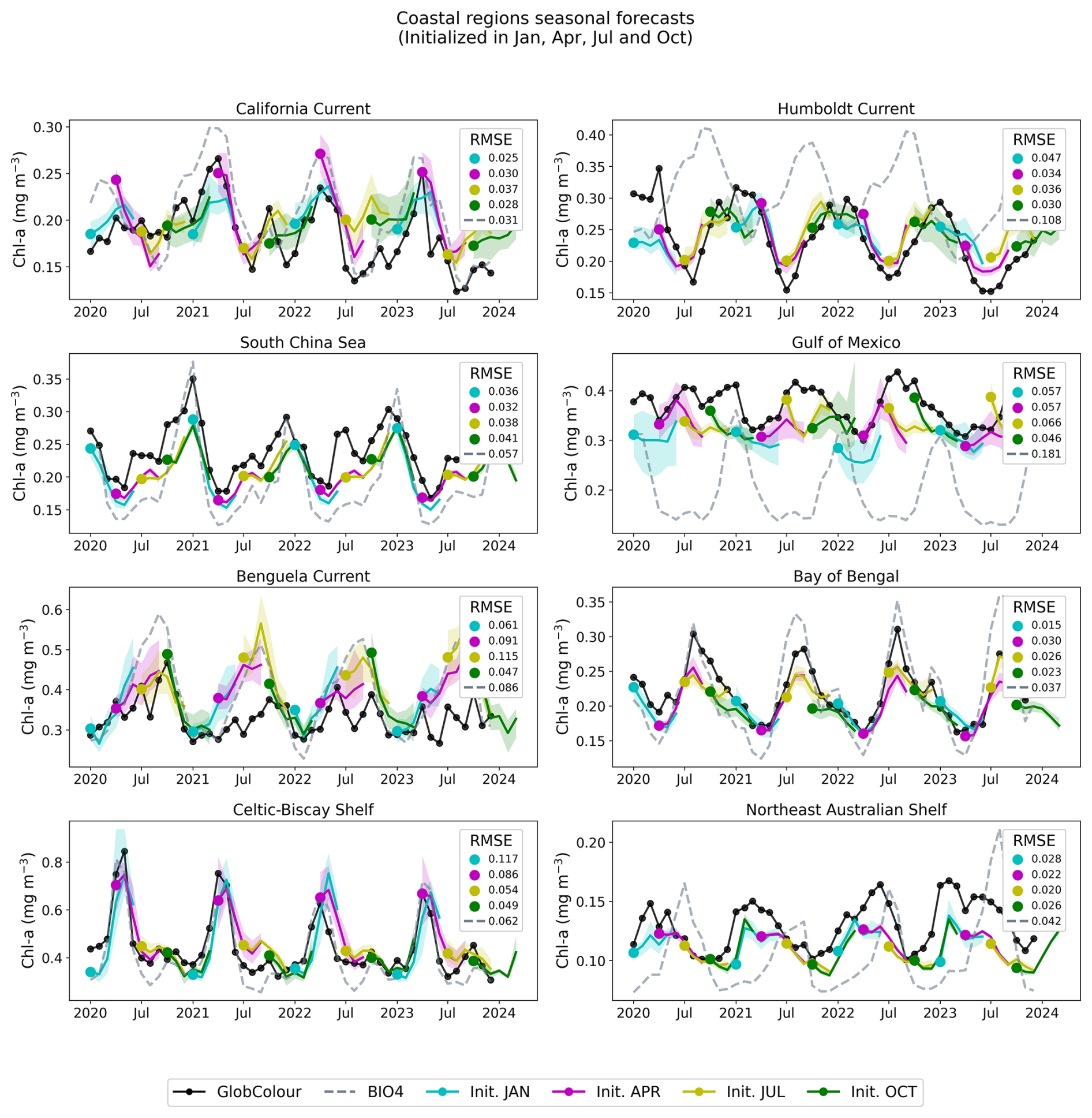
Figure 13 Regional, coastal forecasts. The figure shows GlobColour (black), BIO4 (dashed lines), and the ensemble average and standard deviation of the neural network predictions initialized on January, April, July, and October.

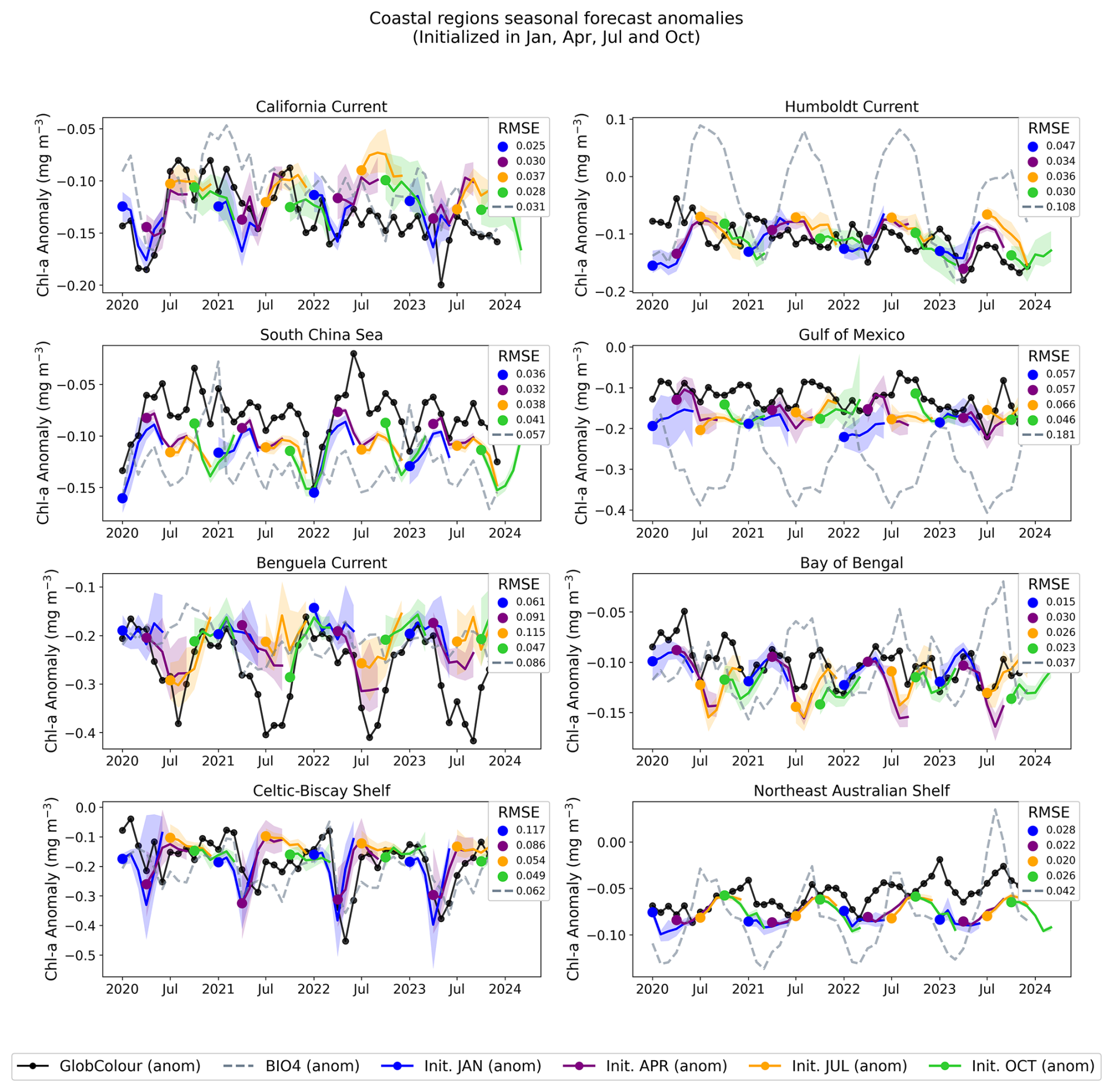
Figure 14 Regional, coastal forecasted anomalies. The figure shows the GlobColour anomaly (black), corresponding BIO4 anomaly (dashed lines), and the ensemble average and standard deviation of forecasted anomalies initialized in January, April, July, and October.

Across regions, the seasonal predictions generally reproduce the observed seasonal cycle and often track GlobColour more closely than BIO4 in terms of magnitude and amplitude. Nonetheless, skill is not uniform and performance varies by region and initialization month, with larger discrepancies often occurring during the peak of the bloom. Note that the RMSE displayed in Figs. 12 and 14 is identical to that of the raw-value figures (Figs. 11 and 13) because the anomalies are computed by subtracting the same monthly GlobColour climatology from both the forecasts and the reference.

The anomaly plots reveal which deviations from the seasonal cycle the model successfully reproduces. The time series demonstrate that forecasts capture departures from the seasonal cycle with varying skill across initialization months and regions, and some cases exhibit consistent offsets or systematic biases. For example, in the South Pacific, predicted anomalies align more closely with BIO4 than with observations, suggesting that shared errors may tied to limitations in the physical input set, or may be predominantly driven by processes that we are either not modeling or struggling to represent.

Notably, in coastal regions such as the Celtic-Biscay Shelf, the South China Sea, the California Current, and the Bay of Bengal, the forecasts capture the overall trend and temporal evolution of the observed anomalies, despite not always matching absolute magnitudes.

Figure 15 shows Hovmöller diagrams, which visualize the evolution of the field as a function of time and one spatial dimension (latitude in this case). The plots summarize the spatiotemporal evolution of surface chl a, making it easier to compare bloom timing, propagation, and amplitude across models. The SEAS5- and GLORYS12-driven neural-network predictions are broadly similar across regions, but the Hovmöller format makes it possible to identify subtle shifts in the timing, latitude/extent, and amplitude of peak concentrations that are likely to contribute to the regional skill degradation highlighted in Fig. 8. BIO4's tendency to overestimate chl a magnitude, is apparent as systematically elevated values relative to GlobColour. These diagrams also highlight interannual variability: despite the dominant seasonal cycle, year-to-year differences in the timing and intensity of blooms are visible. The neural-network predictions exhibit variation across years rather than repeating a purely climatological seasonal pattern, even though these do not always align with the observed deviations from the seasonal cycle.

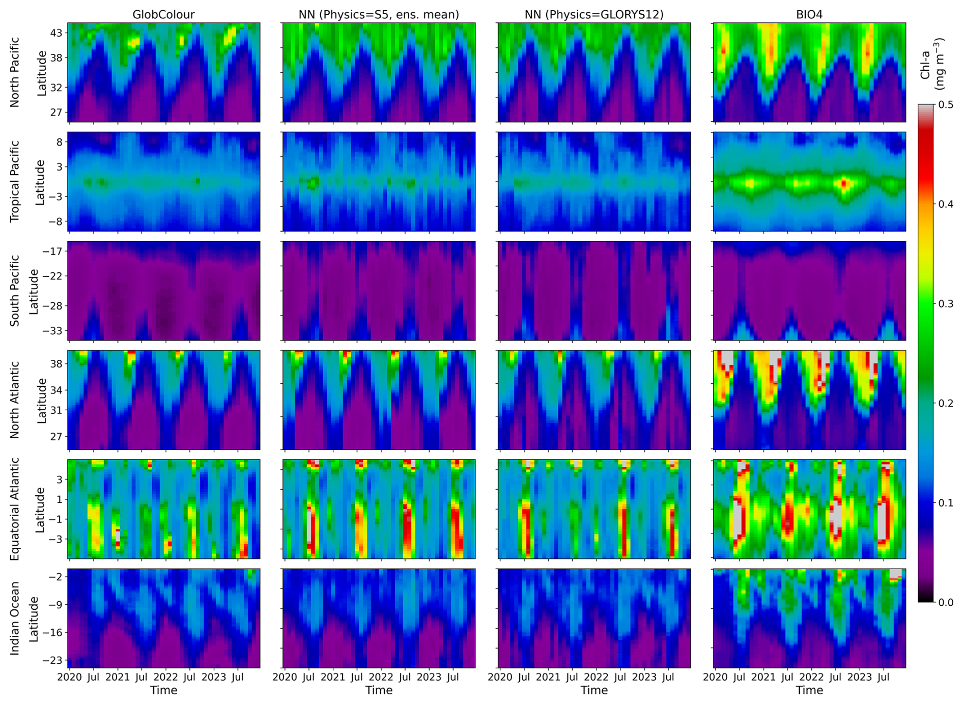
Figure 15 Hovmöller diagrams showing time vs. latitude for each open-ocean region. Columns show (1) the GlobColour reference, (2) the ensemble-mean lead-1 prediction forced by SEAS5 physics, (3) the corresponding prediction forced by GLORYS12 physics, and (4) the BIO4 output.

To investigate how error evolves through the seasonal cycle, Figs. 16 and 17 show RMSE as a function of calendar month for each region. Here, RMSE is computed separately for each calendar month using all valid grid points within the region over 2020–2023 (i.e. not averaged across months like we do in Fig. 10).

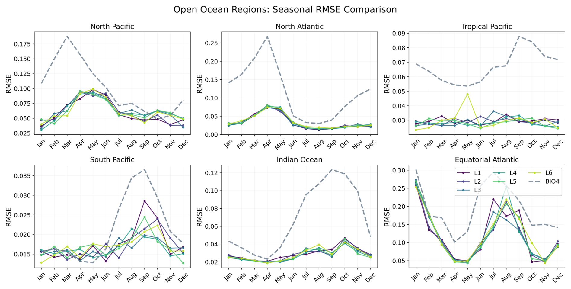
Figure 16 Seasonal evolution of the RMSE for each open-ocean region, comparing BIO4 (dashed lines) with the neural-network seasonal forecasts at lead times 1–6 (L1–L6).

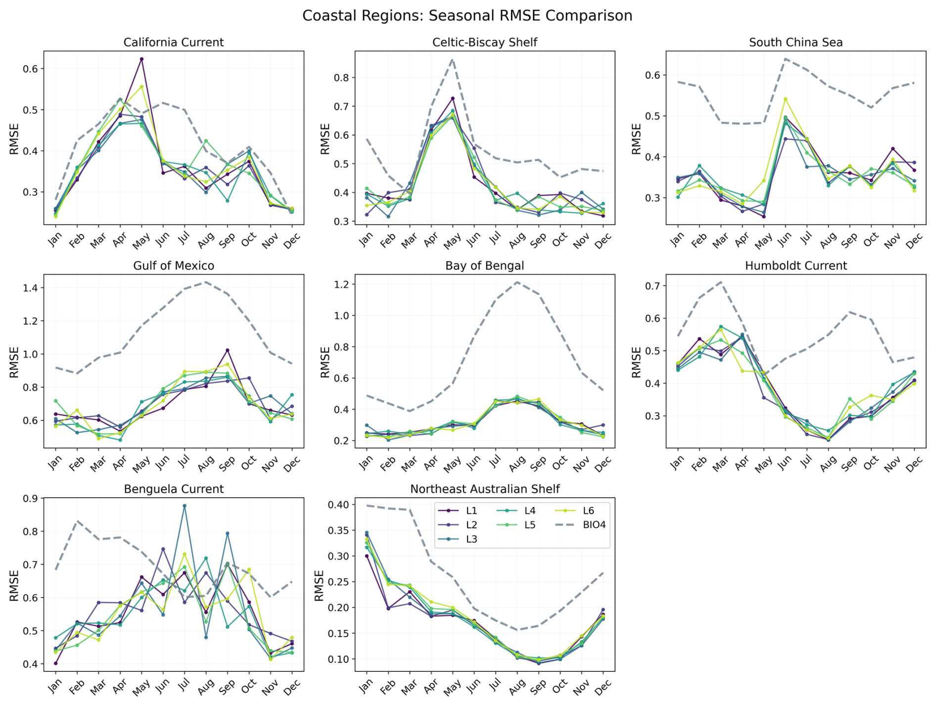
Figure 17 Seasonal evolution of the RMSE for each coastal region comparing BIO4 and seasonal forecasts at L1–L6.

Both the neural network and BIO4 exhibit increased errors during bloom peaks. Northern-hemisphere regions show larger RMSE in the first half of the year, while southern-hemisphere regions peak later, consistent with hemispheric seasonality. This behavior is expected because bloom peaks concentrate the largest amplitudes and strongest spatiotemporal gradients, in RMSE these timing offsets or amplitude damping near the peak translate into large squared errors. The fact that both the neural and process-based models show similar seasonality in error suggests that peak-bloom conditions may be intrinsically harder to predict, potentially reflecting sensitivity to rapidly evolving states and/or drivers that are not explicitly represented, rather than model class alone. However, this seasonal structure is not uniform across regions or between the two models. For example, in the Tropical Pacific the neural-network RMSE shows little seasonal variation compared to BIO4, while in the Humboldt Current BIO4 error has a secondary late-year peak that is not mirrored by the neural model, and the Benguela Current shows a different seasonal pattern. These differences suggest different sources of uncertainty and region-specific dynamics, and that accuracy might be constrained by different representations (or omission) of key drivers.

4 Discussion

We introduced a lightweight, data-driven approach for reconstructing near-global surface chl a from only four physical predictors (MLD, SSH, SSS and SST) and for extending this capability to seasonal forecasting by using forecasted physical ocean states as input. Despite its simplicity, the method achieves high correlation and low error across many regions, while remaining computationally efficient: the network can be trained in a few hours on a single GPU and can produce $\mathrm{1}/\mathrm{4}$°, six-month forecasts within minutes. This makes the framework attractive for rapid generation of large-scale predictions, and in contexts where computational cost is a primary constraint.

Our approach aligns with previous studies that have demonstrated the potential of using physical ocean variables and machine learning for chl a reconstruction (Sauzède et al., 2017; Martinez et al., 2020; Roussillon et al., 2023; Chen et al., 2024). By applying it to forecasted physical ocean states, we further expand the utility of this approach to forecasting, offering a simple yet useful framework for seasonal, near-global surface chl a predictions. Our model focuses solely on surface chl a, but this variable can be used as a proxy for phytoplankton biomass and variability in primary productivity, and it has the advantage of being more readily verifiable from observations. Skillful surface chl a reconstructions and forecasts can help support the study of ecosystem responses to climate variability, and resource-management use cases that depend on these large-scale indicators. At the same time, we acknowledge that important subsurface processes and vertical structure are not represented in our approach, and so this framework would fall short whenever information about the vertical distribution of biomass is required, such as in the presence of a Deep Chlorophyll Maximum (DCM).

Across the 2020–2023 evaluation period, the seasonal forecasts maintain spatially coherent skill even with a six-month lead time (Fig. 8). Regionally, Pearson correlations generally remain high and show limited degradation with lead time (Fig. 9), while RMSE (Fig. 10) is consistently lower than BIO4, a state-of-the-art process based model. The relatively weak degradation that we see with increasing forecast horizon likely reflects that much of the skill is carried by large-scale, slowly varying components, and broad physical states that retain useful information across the 1–6 month range. The time-series and Hovmöller diagnostics (Figs. 11–13 and 15) indicate that the model reproduces the dominant seasonal cycle while exhibiting year-to-year variability, and that it captures the timing and magnitude of major bloom events in many regions. Errors nevertheless peak during bloom maxima (Figs. 16 and 17), potentially due to heightened sensitivity to rapidly evolving physical conditions, or to drivers that are not explicitly represented in our input set.

Our approach retains useful skill in the large-scale evolution of surface chl a, even when driven by forecasted physics that differ from the reanalysis used for training. The similarity between SEAS5- and GLORYS12-driven predictions (Fig. 15) suggests that the method is not tightly tied to a single source of physical data, in spite of the modest skill reduction relative to reanalysis-driven predictions in certain regions (Fig. 8). While this behavior is expected due to forecast errors (Fig. 2) potentially propagating into the chl a reconstruction, a more detailed examination of these differences would be valuable in future work. Such an analysis could identify where loss of skill is dominated by limits in input predictability versus model sensitivity, providing concrete targets for future model development. These could include region or regime-specific training strategies, domain adaptation approaches, or other input corrections aimed specifically at improving robustness.

Limitations

Our framework is intentionally minimalist, and this design choice implies several limitations. First, stricter diagnostics that emphasize interannual variability and small departures from the climatological seasonal cycle are highly phase-sensitive and can penalize even modest changes in timing or small spatial shifts in bloom features. This is expected because removing the seasonal cycle isolates a weaker, noisier signal, and because the monthly evaluation record, with only 48 time steps, is relatively short. In addition, limited predictability in the forecast physical anomalies can further constrain skill. We therefore emphasize metrics (RMSE and Pearson correlation on the raw fields) that better reflect our main objective, which was reproducing realistic magnitudes and large-scale spatiotemporal evolution of surface chl a in a resource-efficient manner. Performance in more complex scenarios where accurate reproduction of anomalies and outliers is crucial would likely require enhancements beyond the minimalist setup presented here. A more systematic treatment of interannual skill would also require a more methodological assessment of SEAS5 skill with respect to anomalies, in order to evaluate how forecast errors might propagate into the chl a reconstruction. A similar decomposition of skill for the process-based benchmark would enable a more principled comparison of performance between approaches

Second, we deliberately restrict predictors to four variables (MLD, SSH, SSS, and SST) that are available in both reanalyses and seasonal forecasts, and in order to keep the framework lightweight and readily deployable, but by doing so, we neglect drivers that can be crucial. These include irradiance (PAR), a key driver in light-limited regimes, winds and mixing variability not fully summarized by monthly MLD, and biogeochemical state variables (e.g. nutrients). As a result, forecast errors will increase in regimes where chl a variability is strongly controlled by factors not captured in the input set, such as light limitation and nutrient supply. Several studies suggest that interannual predictability in chl a is closely linked to biogeochemical drivers, which can exhibit longer predictability than physical variables alone (Séférian et al., 2014; Rousseaux et al., 2021; Park et al., 2019b; Ham et al., 2021; Frölicher et al., 2020). As with any modeling approach, trade-offs are inevitable. While biogeochemical variables can carry higher uncertainties, they may also capture important feedbacks not fully represented by physical drivers. Future versions of this approach could therefore benefit from a more principled investigation of predictor uncertainty and sensitivity analyses to systematically incorporate any additional relevant physical and biogeochemical inputs.

Third, the neural network design is intentionally lightweight, but this comes at the cost of potentially failing to capture the full intricacy of the underlying processes. We used a simplified U-Net architecture and a month-conditioned strategy implemented as twelve separately trained networks (one per initialization month) rather than a single unified model. While this choice simplifies training across the seasonal cycle, it increases system complexity and can introduce month-to-month inconsistencies because the mapping from physics to chl a is learned independently for each network. A natural extension would be to adopt a more robust architecture that explicitly conditions on month and lead time through a shared-backbone design.

Furthermore, while MSE is a standard choice for regressive neural networks such as this one, its focus on minimizing error can lead to overly smooth predictions that tend toward the mean. This can result in the loss of fine-scale detail in regions with high variability, and an overall impact on the realism of the model's predictions. Future work could mitigate this by adopting more robust learning objectives and/or by increasing architectural capacity. In addition, the forecast “ensemble” presented here is derived from the propagation of uncertainty from the SEAS5 physical ensemble through a deterministic chl a reconstruction. It does not explicitly represent chl a uncertainties, and it inherits any shared biases and limits in the physical forecast. A more complete approach would require the inclusion of more comprehensive sources of uncertainty and the perturbation of these within the predictive framework.

Finally, data-driven methods like ours, which learn directly from observations, can better reproduce observed chl a magnitudes and avoid some of the systematic biases that arise from uncertain parameterizations in process-based models (manifested as systematic overestimations relative to GlobColour in the case of BIO4). Nonetheless, this same minimalistic design, which emphasizes good skill in the raw fields in its current form, may also limit performance. Mechanistic biogeochemical models, by enforcing dynamical and biogeochemical consistency across variables, may be more robust for extrapolation beyond the observational regime, whereas purely data-driven approaches may degrade under distribution shift or in regimes that are poorly represented in the training data.

5 Conclusions

Our resource-efficient, data-driven methodology demonstrates competitive results for the estimation of seasonal surface chl a at a near-global scale. This is done by using MLD, SSH, SSS and SST data as input for a lightweight, U-Net-like neural network that is trainable in a matter of hours on a single GPU. Our method can be used to reconstruct historical chl a patterns (i.e. by using a reanalysis as input), or to generate predictions based on easily accessible forecast data. While future work is needed to better quantify and improve performance on interannual variability, these predictions show low error and high correlation to observations across different regions and lead times. The method is computationally efficient, and can be easily expanded to improve accuracy and extend its capabilities to other satellite-derived ocean-colour variables.