Improving coastal ocean pH estimates through assimilation of glider observations and hybrid statistical methods

Ocean acidification monitoring and carbon accounting require accurate estimates of marine carbonate system variables, particularly in dynamic coastal regions where observations remain sparse. This study presents an approach to improving carbonate system state estimates in the California Current System through the assimilation of underwater glider observations with both dynamical and statistical models. We implement a 4D-Var data assimilation system that jointly assimilates physical variables, chlorophyll, and glider-based pH and alkalinity data into a regional coupled physical-biogeochemical model. In our experiments, the assimilation of physical variables and chlorophyll alone has limited impact on pH and other carbonate system estimates, while the joint assimilation including pH and alkalinity variables successfully improves these estimates. Cross-validation experiments further demonstrate that the joint assimilation typically also improves estimates near the observation network, although downstream advection of increments can occasionally degrade results. We also show that hybrid estimates that combine the output of the dynamical, physical ocean model with a statistical model produce accurate carbonate system estimates without requiring a biogeochemical model. This finding suggests that physical ocean models and data assimilation systems can obtain reasonable carbonate system estimates by combining statistical methods with model estimates of temperature and salinity. Our carbonate system data assimilation setup relies on the combined assimilation of pH and alkalinity data to obtain reliable state estimates. Because alkalinity is not yet routinely measured by gliders, we utilize statistically estimated alkalinity values and examine the limitations of this approach in our study.

1 Introduction

The ocean plays a central role in modulating Earth's carbon cycle, acting as a major carbon reservoir and sink for anthropogenic emissions. Recent estimates indicate that the ocean has removed approximately one quarter of total anthropogenic carbon emissions (Friedlingstein et al., 2023). This increased uptake of atmospheric CO₂ results in decreased ocean pH and associated changes in carbonate system equilibrium through ocean acidification. While the coastal ocean globally acts as a sink for atmospheric CO₂, there is substantial regional variability (Bauer et al., 2013; Roobaert et al., 2019), with uptake largely modulated by biological carbon fixation and the biological response to climate-induced changes (Mathis et al., 2024). To understand and predict changes in ocean carbonate chemistry, the scientific community increasingly relies on coupled physical-biogeochemical ocean models (Fennel et al., 2019; Kwiatkowski et al., 2020; Fennel et al., 2022). These models combine estimates of ocean circulation dynamics with biogeochemical processes to provide state estimates of carbonate system variables and their temporal evolution.

Eastern boundary upwelling systems, such as the California Current System (CCS), represent biologically highly productive regions characterized by complex coastal processes operating across multiple spatial and temporal scales (Checkley and Barth, 2009). The nearshore environment in the CCS naturally experiences low pH and reduced oxygen conditions in response to coastal upwelling (Cheresh and Fiechter, 2020). While the southern CCS shows increased acidification consistent with global surface ocean trends (Wolfe et al., 2023), there are substantial regional differences in alongshore mean pH and dissolved oxygen distributions (Cheresh and Fiechter, 2020). Understanding these regional patterns and their underlying drivers requires both observational data and sophisticated modeling approaches. Regional ocean models have proven successful at simulating the physical and biogeochemical dynamics of the CCS (Veneziani et al., 2009; Fiechter et al., 2018; Deutsch et al., 2021).

Despite the ocean's crucial role in carbon cycling, marine carbonate system variables remain poorly observed. Although millions of surface ocean pCO₂ measurements exist (Bakker et al., 2022), subsurface measurements of pH, alkalinity, or dissolved inorganic carbon (DIC) are comparatively sparse (Land et al., 2023). This observational gap is particularly challenging in dynamic coastal regions such as the CCS, where high spatial and temporal variability demands dense sampling. Underwater gliders have been shown to be a particularly effective autonomous platform to provide sustained, high-resolution data in a cost-effective manner in the coastal ocean (Rudnick, 2016). For example, the California Underwater Glider Network (CUGN) has near-continuously occupied three across-shore transects in the Southern to Central California coast since 2007, and two more transects were added recently to the network (Rudnick et al., 2017). The CUGN gliders measure temperature, salinity, water velocity, chlorophyll fluorescence, and more recently, oxygen starting in 2017 (Ren et al., 2023). There have been several examples where underwater gliders were equipped with pH sensors (Saba et al., 2019; Takeshita et al., 2021; Hemming et al., 2017), providing an opportunity to collect high spatiotemporal, subsurface marine carbonate system variables in the coastal ocean. In particular for the CCS, Takeshita et al. (2021) integrated a Deep-Sea-DuraFET pH sensor (Johnson et al., 2016) onto a Spray glider, and operated it along Line 67 in 2019, one of the transects occupied by the CUGN. Ongoing efforts to integrate pH sensors into the CUGN glider fleet promises new opportunities for monitoring ocean acidification and improving model estimates.

Data assimilation (DA) describes the process of merging models and observations to obtain accurate and gapless estimates of the ocean state (Edwards et al., 2015; Martin et al., 2024). The challenge of obtaining reliable marine carbonate system state estimates has motivated various DA approaches. Several studies have explored the assimilation of carbonate system variables to improve model estimates of climate-relevant parameters such as air-sea CO₂ exchange. Visinelli et al. (2016), using a global state estimation setup based on the 3D-Var DA technique, found that assimilating physical observations alone can either improve or deteriorate estimates of alkalinity and DIC depending on the region, while joint assimilation of alkalinity and DIC improved overall estimates of air-sea CO₂ flux, though not consistently across all regions. Carroll et al. (2020) employed a global coupled physical-biogeochemical model with adjoint-based physical DA and a Green's function approach for biogeochemical DA to estimate carbonate system dynamics and CO₂ air-sea flux across seasonal to multidecadal timescales. Turner et al. (2023) utilized ensemble optimal interpolation DA to estimate upper ocean carbon content based on temperature and salinity observations, while Verdy and Mazloff (2017) produced biogeochemical state estimates for the Southern Ocean by assimilating both physical data and various carbonate system and oxygen observations.

Recent work has also highlighted that carbonate system variables can be accurately estimated, particularly in the subsurface, using statistical models (also known as empirical algorithms) with inputs of more commonly measured properties such as temperature, salinity, oxygen, and location (Alin et al., 2012; Bittig et al., 2018; Carter et al., 2021). These models, such as the Empirical Seawater Property Estimation Routines (ESPER; Carter et al., 2021) and CANYON-B (Bittig et al., 2018) are trained on high-quality shipboard data (Olsen et al., 2020), using statistical regression or machine learning approaches. Using the output of dynamical ocean models as inputs to these statistical models provides an opportunity to produce gapless state estimates of the marine carbonate system. These hybrid estimates, which feed the state estimates of dynamical models into statistical models, stand to benefit from DA, which aims to improve dynamical model estimates.

In this study, we integrate underwater glider-based carbonate system variables and oxygen data into a DA system based on a regional physical-biogeochemical ocean model for the CCS. In particular, we utilize algorithm-based estimates for pH, DIC, and alkalinity from 2019 using CUGN glider temperature, salinity, and oxygen as inputs. Additionally, we also utilize direct sensor measurements of pH and oxygen from one transect along Line 67 (Takeshita et al., 2021). Our reference DA experiment jointly assimilates temperature, salinity, and sea level anomaly (SLA) data with satellite chlorophyll a (hereafter simply chlorophyll) in a 4D-Var-based state estimation setup similar to that in Mattern et al. (2017, 2018). Through a series of experiments, we examine the effects of assimilating glider-based data alongside the reference data.

Building on previous DA work and recent glider-based pH and oxygen data, this study pursues three main goals: First, we examine the impact of jointly assimilating carbonate system variables (primarily pH and alkalinity) and oxygen with physical and chlorophyll observations. Second, we assess the influence of assimilating different data subsets on the model's state estimates, examining the relative importance of various observation types and their interactions in the assimilation system. Third, we investigate whether integrating ROMS model temperature and salinity estimates with the ESPER statistical model can produce useful hybrid estimates of carbonate system variables, potentially offering a practical approach for carbonate system state estimation based on physical ocean models and DA systems. With our DA framework, we ultimately aim to address the need for improved coastal carbonate system monitoring and the broader challenge of developing efficient methods for ocean acidification tracking in dynamic coastal environments.

2 Methods

2.1 Model domain and physical setup

Our model is based on version 3.7 of the Regional Ocean Modeling System (ROMS; Haidvogel et al., 2008), a primitive equation, hydrostatic, free surface regional ocean physical circulation model. The model domain is designed to simulate physical and biogeochemical dynamics in the CCS. It extends from 30 to 48° N, and longitudinally from the U.S. west coast to 134° W, with a horizontal resolution of 0.1° × 0.1° (resulting in a ≈ 10 km resolution) The model is vertically divided into 42 terrain-following layers with a higher resolution near the ocean surface. Our implementation uses the Coupled Ocean Atmosphere Mesoscale Prediction System (COAMPS; Doyle et al., 2009) for physical forcing at the surface (wind, longwave solar radiation, air temperature, pressure, and humidity). Boundary conditions for the physical model are provided by Copernicus Global $\mathrm{1}/\mathrm{12}$° reanalysis (GLORYS; Jean-Michel et al., 2021). The GLORYS product is further used to nudge model temperature and salinity toward their reanalysis values in a 1° wide “sponge” region along the open model boundaries. This physical model setup closely follows that in previous studies, such as Veneziani et al. (2009) and Mattern et al. (2017).

2.2 The NEMUCSC biogeochemical model

As a biogeochemical model, we use the NEMUCSC model, an extension of the North Pacific Ecosystem Model for Understanding Regional Oceanography (NEMURO; Kishi et al., 2007). Our NEMUCSC configuration has been extended from the setup presented in Mattern et al. (2017) with carbon and oxygen cycling and phytoplankton photoadaptation (i.e., dynamic nitrogen to chlorophyll ratios for phytoplankton, which we detail below).

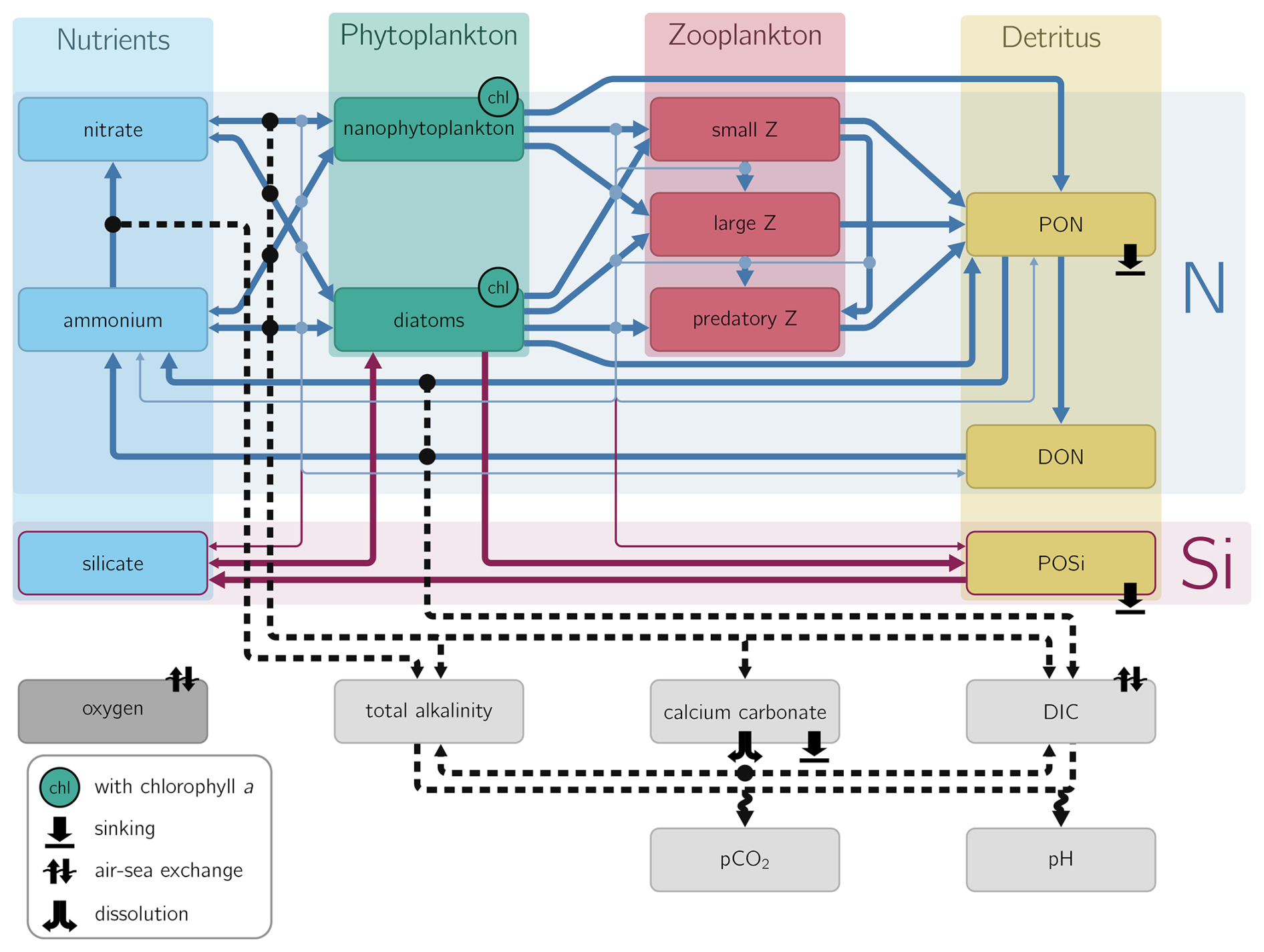
Figure 1 NEMUCSC model diagram: Outline of the NEMUCSC model variables and pathways connecting them. Nitrogen and silicate-based variables are outlined in blue and red, respectively, carbonate system variables are shown in light gray. Pathways between nitrogen and silicate-based variables, indicated by thick solid arrows for major processes (e.g. grazing) and thinner solid arrows for minor processes (e.g. particulate matter exudation due to sloppy/inefficient grazing) transfer matter between variables. In contrast, matter is not transferred between carbonate system variables; instead, biogeochemical processes affecting a carbonate system variable lead to an increase or decrease of that variable, the connection between processes and affected carbonate system variable is shown by black dashed arrows. Pathways affecting model oxygen are not shown.

The base NEMUCSC model accounts for a range of biogeochemical constituents and interactions in the ecosystem, including: (1) three limiting macronutrients (nitrate, ammonium, and silicate); (2) two phytoplankton functional types (nanophytoplankton and diatoms); (3) three zooplankton size classes (microzooplankton, mesozooplankton, and predatory zooplankton); and (4) three detritus pools (dissolved and particulate organic nitrogen and particulate silica). The NEMUCSC carbon extension, presented in Cheresh and Fiechter (2020) with refinements to alkalinity and carbon dynamics described in Green (2025), adds dissolved inorganic carbon (DIC), total alkalinity, and calcium carbonate variables. It computes ocean pH and pCO₂ based on the OCMIP carbonate chemistry (Fig. 1).

The second extension to the NEMUCSC model adds a chlorophyll variable for each of the two nitrogen-based phytoplankton variables. The photoadaptation model presented in Jackson et al. (2017) is used to dynamically adjust the stoichiometric ratio of nitrogen to chlorophyll for the two phytoplankton functional types represented in the model, assuming a constant nitrogen-to-carbon ratio based on the Redfield ratio.

We further expanded the code required by the DA (NEMURO's tangent-linear and adjoint code; see Mattern et al., 2017) to fully support the extended model and permit the assimilation of chlorophyll, oxygen and carbonate system variables. For DA, we added a “total chlorophyll” variable which is the sum of diatom chlorophyll and nanophytoplankton chlorophyll, so that chlorophyll observations can be directly assimilated, informing both phytoplankton functional types. Following Song et al. (2012) and Mattern et al. (2017), chlorophyll is log-transformed in the DA procedure. A log-transformation is not applied to pH, alkalinity, DIC, oxygen or the physical variables for which we also assimilate data in this study.

For the carbonate system variables DIC and alkalinity, as well as oxygen, nitrate and silicate, boundary conditions are created using statistical relationships from ESPER, based on temperature and salinity boundary values. Following a comparison with climatological nutrient values from the World Ocean Atlas (Garcia et al., 2024), nitrate boundary values in the mixed layer were reduced to match World Ocean Atlas values, and to prevent unrealistically high nitrate input through the boundaries. To further prevent unrealistic values for other variables, boundary conditions for the remaining BGC variables are set to low values that roughly match model estimates near the boundaries. For the year of our experiments, 2019, atmospheric pCO₂ is set to a constant value of 400 ppm.

2.3 Data used in the assimilation and verification

In this study, we use a variety of satellite, glider, and float observations, complemented by estimated data derived from statistical relationships using an average of three algorithms (ESPER-LIR, ESPER-NN, and CANYON-B). We conducted a series of experiments in which various data subsets were excluded from the assimilation process to examine their influence on model state estimates. Furthermore, we used model state estimates with and without DA and ESPER-LIR to derive hybrid (dynamical model + statistical model) state estimates.

The datasets are classified into three broad categories:

1. Reference dataset: this represents what is typically assimilated in a coupled physical-BGC model, encompassing:

   • Temperature data from satellites

   • In situ observations of temperature and salinity from gliders, including gliders from the California Underwater Glider Network (CUGN), and floats

   • Satellite-based sea level anomaly (SLA) data

   • Chlorophyll data derived from satellite ocean color

2. Extended reference dataset: this supplements the reference data by incorporating

   • Oxygen observations from the CUGN glider deployments

   • Estimated values of pH, alkalinity, and DIC obtained as an average of three statistical algorithms with inputs of glider temperature, salinity, and oxygen observations

3. pH-sensor glider line dataset: this dataset is based on several deployments of a glider with an in situ pH sensor for Line 67, extending westward out of Monterey Bay. It includes:

   • Temperature, salinity, pH, and oxygen observations

   • Estimated values for alkalinity using algorithms and estimated DIC by combining measured pH and estimated alkalinity

All data used in our DA experiments are freely available. The sources for the datasets and their association with the categories are listed in Table 1.

(CMEMS, 2022a)(CMEMS, 2022b)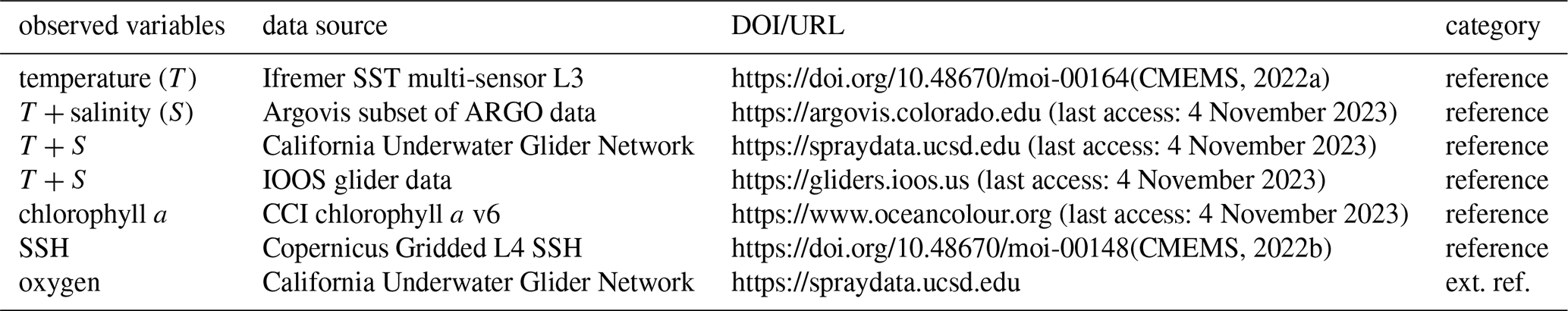

Table 1 The data used for assimilation and verification.

In our DA experiments, we assimilate so-called super-observations, which are observations that are averaged based on the model grid and time stepping so that there is at most one observation of the same type in each model grid cell and time step. The use of super-observations is standard in DA applications (Martin et al., 2024); for dense data sets, such as glider-based observations, the process of creating super-observations can reduce the number of data points considerably. However, in quantitative evaluations that use glider-based observations, we use the original observations, not the super-observations. We adopt this approach for two reasons: first, we are more interested in improving the fit to the full set of observations rather than the model grid-dependent aggregated data. Second, for visualization purposes, a denser set of observations better reveals observed features. Interestingly, the overall model fit to the original glider observations is typically better than for the super-observations, a phenomenon we discuss in more detail in Sect. 4. Because only super-observations are assimilated, we often drop the “super” prefix and refer to the assimilated data simply as “observations” or “data”. When needed, we use the term super-observations to avoid ambiguity.

2.4 Data assimilation experiments

In this study, we conducted several DA experiments to systematically investigate the impact of assimilating different observation subsets. Table 2 provides an overview of all experiments and the data assimilated in each.

Table 2 Experiments and assimilated data.

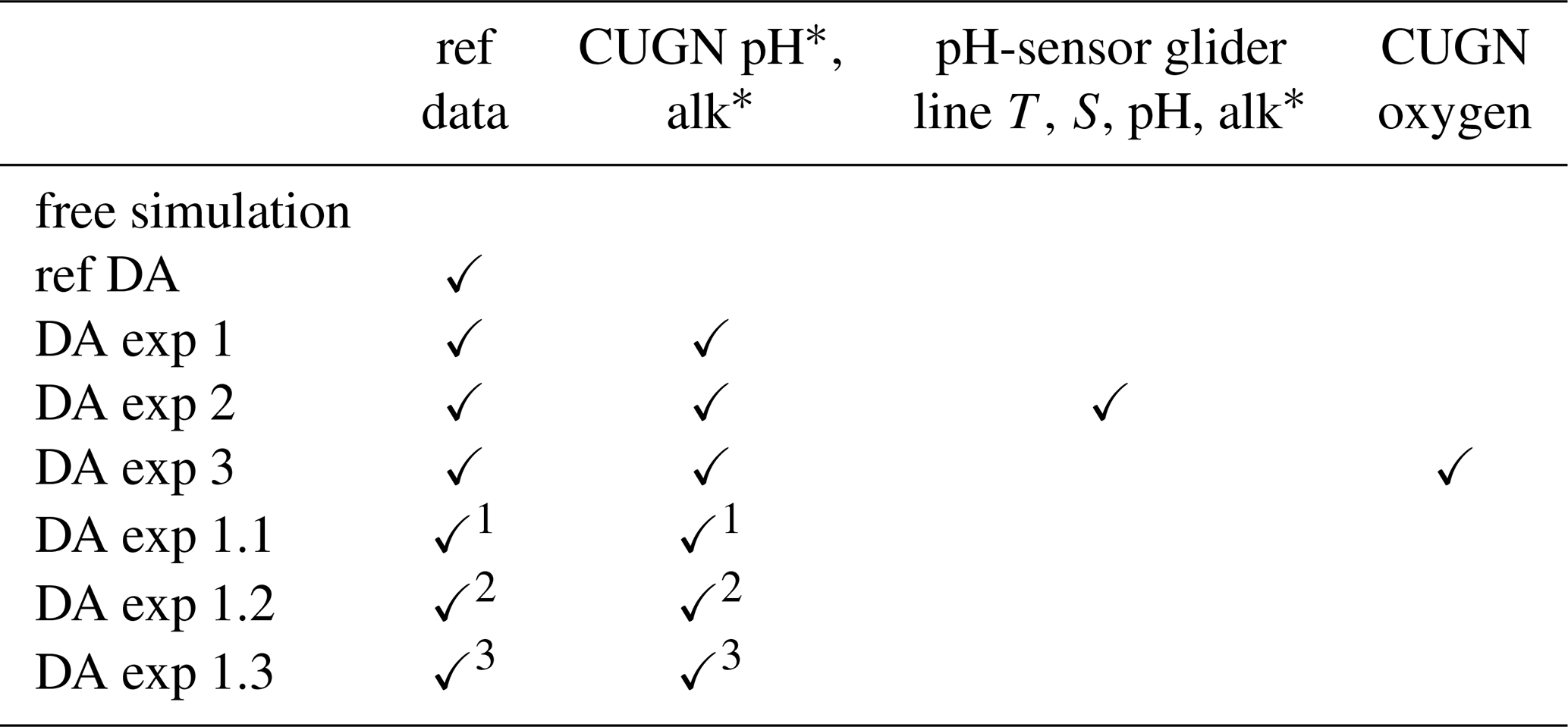
^∗ Data not directly measured, estimated based on statistical relationships.
¹ Excluding CUGN L67Mar. ² Excluding CUGN L67Jul. ³ Excluding CUGN L67Oct.

To establish a baseline, we use two reference simulations: a non-assimilative “free simulation” and a reference DA experiment. The free simulation does not assimilate any observations and is solely driven by the coupled physical-biogeochemical model. Our reference DA experiment represents a typical joint physical-biogeochemical DA approach. It assimilates remotely sensed and in situ temperature and salinity data, satellite sea level anomaly (SLA), and satellite-derived chlorophyll. This experiment serves as a benchmark for current physical-biogeochemical DA without any carbonate system observations.

Building upon the reference DA, we conducted three main experiments that progressively incorporate additional observation types: DA exp 1 assimilates all reference data plus CUGN pH and alkalinity estimates. This experiment examines the impact of jointly assimilating carbonate system variables with the standard physical and chlorophyll data.

DA exp 2 builds on DA exp 1 by additionally assimilating pH-sensor glider line temperature, salinity, pH, and alkalinity data. This experiment aim is to examine the model estimates achievable through direct assimilation of the pH-sensor glider data , compared to the assimilation of neighboring CUGN pH and alkalinity in DA exp 1.

DA exp 3 assimilates all reference data plus CUGN pH, alkalinity, and oxygen data. This experiment investigates the impact of including oxygen observations in the assimilation framework.

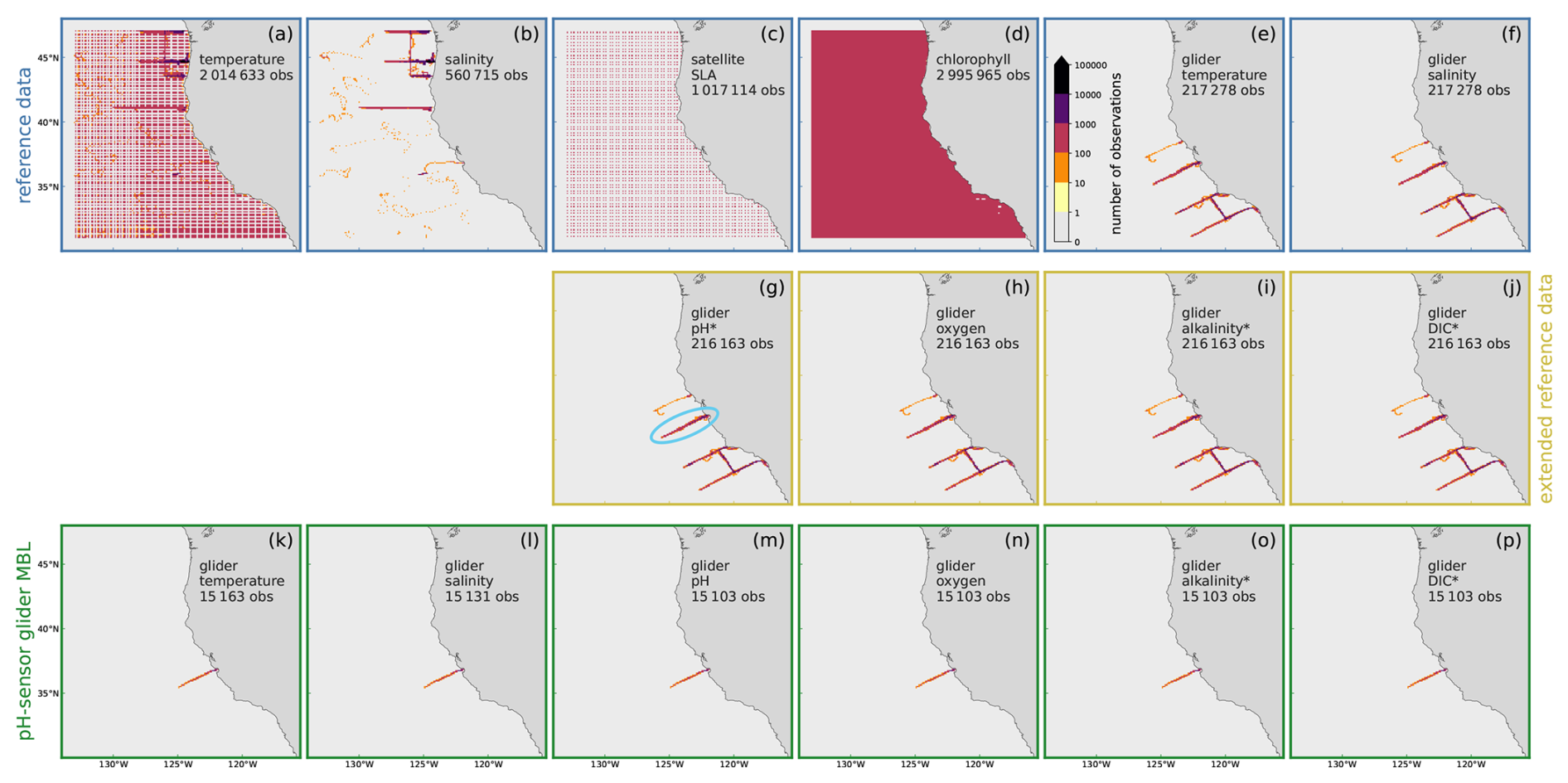
Figure 2 Histogram of observation locations: 2-dimensional histogram showing the number of observations and their horizontal location on the model grid for each observation type. The observations are divided into 3 categories: (a–f) The reference data contains mostly remotely sensed observations, augmented by glider- and float-based observations of temperature and salinity. (g–j) The extended reference further includes glider-based data for pH, oxygen, alkalinity and DIC. (k–p) The pH-sensor glider dataset contains glider data from independent deployments. Asterisks (^∗), denote data that was not directly measured, but obtained from other measurements using statistical relationships. The light blue ellipse in panel (g) marks the Line 67.

To assess the spatial influence of the pH DA and validate our approach, we conducted three cross-validation experiments: we focused on three CUGN glider transects out of Monterey Bay along Line 67 (see highlighted line in Fig. 2g) in different seasons (starting in late March, July, and October 2019). During each transect, the glider moved westward out of Monterey Bay, covered the full extent of the line, and returned nearshore. We denote these three lines as CUGN L67Mar, CUGN L67Jul, and CUGN L67Oct (started in March, July, and October 2019, respectively) and performed an experiment excluding the data for each line. DA exp 1.1, 1.2, and 1.3 assimilate all data from DA exp 1 except CUGN L67Mar, L67Jul, or L67Oct data, respectively. These cross-validation experiments allow us to evaluate the model's ability to estimate pH and other variables at locations where observations are withheld from the assimilation.

In addition to these direct assimilation experiments, we create hybrid estimates by using dynamical ocean model outputs as inputs to the ESPER statistical model. ESPER can provide estimates of various biogeochemical seawater properties, including pH, alkalinity, DIC, and oxygen. It generates these estimates based on location information, temperature and salinity, and optionally, additional inputs such as oxygen. We can use the model estimates of temperature and salinity as input to ESPER to obtain pH, alkalinity, DIC, and oxygen estimates. These hybrid estimates, combining the dynamical model with the statistical model, may benefit from physical DA as it improves the temperature and salinity estimates that enter ESPER. We created hybrid estimates using the published version of ESPER (ESPER_LIR V1.01) without any additional training and based on model estimates from

1. the free simulation (ESPER based on temperature and salinity only),

2. the reference DA (ESPER based on temperature and salinity only),

3. DA exp 3 (ESPER based on temperature, salinity, and oxygen).

This experimental design allows us to systematically evaluate the impact of different observation types on model state estimates and to compare direct assimilation with hybrid approaches for generating carbonate system estimates.

2.5 Observation and background error values

The 4dVar DA system requires the specification of observation error and background error values, the latter to quantify the model uncertainty associated with the background model state, prior to performing DA. Previous experience working with joint 4dVar DA for physical and chlorophyll a observations, and differences between the observed variables in the carbonate system submodule and the rest of the model suggest different approaches for specifying error values for these two parts of the model.

Mattern et al. (2018) outlines an iterative technique to adjust observation error and background error values to improve the consistency of prior and posterior error values. The adjustments were shown to have a positive effect on 4dVar performance diagnostics and model performance metrics, such as the forecasting skill. This technique, which we hereafter refer to as a fixed point iteration, or “FPI”, can only be applied to the background error values of directly observed variables or variables with a simple relationship to assimilated observations. In the physical model, the temperature, salinity, and SSH variables are directly observed, which means that the observations of temperature, salinity, and SSH correspond directly to these model variables. Chlorophyll a is also directly observed, but the value of the chlorophyll a variable is a function of, and mostly determined by the values of the model's two phytoplankton variables, diatom and nanophytoplankton. By assuming a constant phytoplankton nitrogen:chlorophyll a ratio, we can create a simple (linear) relationship between the phytoplankton variables and the chlorophyll a observations. This approach permits us, starting from initial estimates, to utilize the FPI to adjust temperature, salinity, SSH, and chlorophyll a observation error values and the background error values for the model variables associated with these observations (see Mattern et al., 2018 for details).

Because the relationship between observations of the carbonate system and model variables is often more complex, the FPI cannot easily be applied to variables of the carbonate system. For example, model pH is a complex, non-linear function of alkalinity, DIC, temperature, and salinity. Thus, we rely on our initial estimates of observation errors and background error values for the carbonate system variables.

Table 3 The observation error values used in the assimilation.

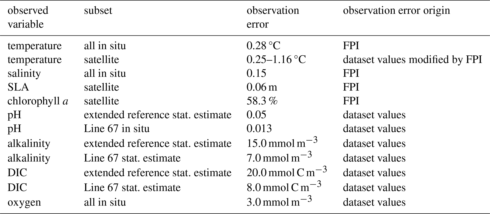
For observation error values, we used the uncertainty values provided with the datasets when available and constant errors otherwise. Specifically, we started with 0.1 °C, 0.05, 10 cm, and 30 % (relative error) as the observation error estimates for in situ temperature, in situ salinity, SSH, and chlorophyll, respectively, when no uncertainty values were provided by the datasets. These values were adjusted using the FPI described above; the resulting error values used in our experiments are listed in Table 3 alongside the error values used for the other observations that were not modified. For oxygen, the reported uncertainty is 0.5 %, which is about 1–1.5 µmol kg⁻¹ at the surface in the CCS (Ren et al., 2023). However, to account for biases due to the response time of the sensor, we use 3 µmol kg⁻¹ in this study. For the Line 67 pH glider, we use 0.013 for pH and the error values reported in Takeshita et al. (2021).

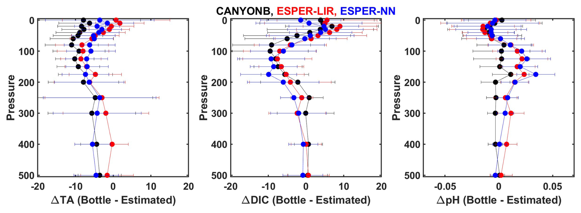
Figure 3 Profiles of measured minus estimated values for alkalinity (left), DIC (middle), and pH (right) using CANYON-B (black), ESPER-LIR (red), and ESPER-NN (blue). The markers represent the median, and error bars represent 1 standard deviation.

The error values for statistically estimated alkalinity, DIC, and pH using T, S, and oxygen as inputs were calculated based on comparisons with discrete samples. We assessed the performance of three algorithms (ESPER-LIR, ESPER-NN, and CANYON-B) using data from three cruises (WCOA 2021 (33RO20210613), 32WF20190511, and 32WF20190723) that span a large part of the model domain (Fig. 3). These cruises were not included in the training datasets for the algorithms and thus represent an independent assessment for the algorithms. We focus on the upper 500 m, as the errors are higher in the upper water column, they provide an upper bound for the error estimate. In general, all three algorithms produced reliable estimates of alkalinity, DIC, and pH across the whole model domain. The median difference was −4.5 µmol kg⁻¹ for alkalinity, −0.1 µmol kg⁻¹ for DIC, and −0.001 for pH, demonstrating small or insignificant systematic bias. Given that there was no clear “best” algorithm in this domain, we chose to average the output of the three algorithms. The error values for these parameters were estimated as the range of the lowest and highest values from the error bars in Fig. 3 and were ±15 µmol kg⁻¹ for alkalinity, ±20 µmol kg⁻¹ for DIC, and ±0.05 for pH. These represent conservative estimates of the errors.

The prescribed background error values (specifying the diagonal entries of the background error covariance matrix) for all model variables are assumed to be constant at the surface and decrease with depth following an S-shaped logistic function (for all variables except SLA, which has no depth-dependence). Below 200 m, where oceanic variability is weaker, background error values are set to approximately 10 % of their magnitude at the surface (following the approach in Mattern et al., 2018).

Table 4 The background error values used in the assimilation. All background error values are constant horizontally and highest at the surface, declining to 10 % of their surface at depth below 200 m (except for SLA which is only defined at the surface). Background error values for diagnostic variables, such as pH, and semi-diagnostic variables, such as diatom chlorophyll a, have little impact on the DA result and are not shown.

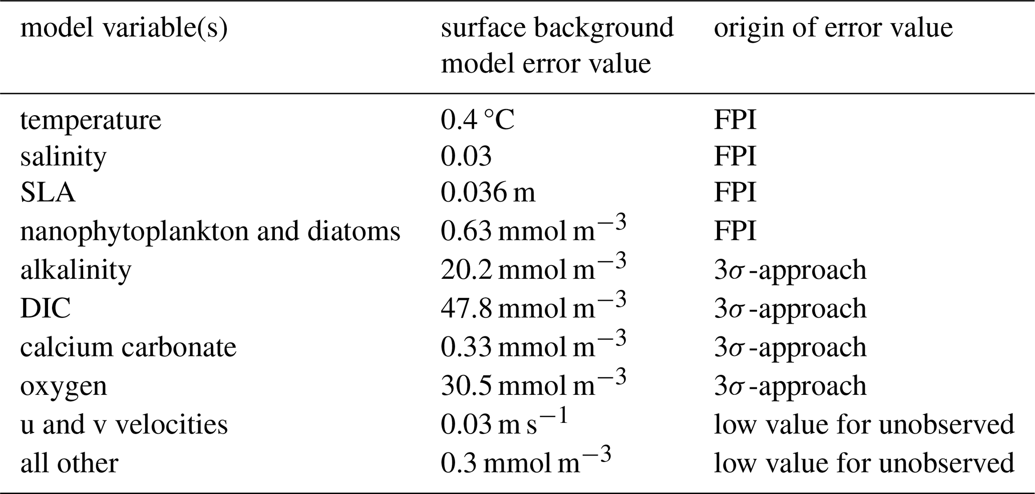
The background error values for temperature, salinity, SSH, diatom, and nanophytoplankton are set using the FPI. For the carbonate system variables and oxygen, we use a long, non-assimilative model simulation to set the surface value: for each variable, we assume that all daily average surface values are contained within a window of ±3 standard deviations from its mean. Thus, we take the difference between the maximum daily average surface value in the simulation and its minimum and divide it by 6 to obtain the standard deviation (this is referred to as “3σ-approach” in Table 4). The background error values for the other model variables are set to low values to prevent large increments to unobserved variables. All surface background error values used in our experiments are listed in Table 4.

2.6 Considerations for assimilating pH data

In a state estimation setting, assimilating pH data (observed or estimated) alone can deteriorate carbon state estimates. This issue arises because, in the model, pH is primarily a function of, and calculated from model estimates of DIC and alkalinity. Different combinations of alkalinity and DIC can yield the same pH value, resulting in model alkalinity and DIC estimates being underdetermined by pH data, analogous to temperature and salinity estimates being underdetermined by density observations in a physical assimilation setting.

In our initial experiments, where we assimilated pH observations alone, state estimates were moved to points in alkalinity-DIC space with the correct pH value. However, the resulting estimates of alkalinity and DIC were largely based on their initial estimates and the prescribed background model error values, rather than reflecting the true state of the system (see also Fig. 5 in Fennel et al., 2023). To move state estimates to the correct point in alkalinity-DIC space, we found it necessary to assimilate two out of the three properties: pH, alkalinity, and DIC.

For this study, we elected to assimilate pH, as it was directly measured on Line 67, and estimated alkalinity because its uncertainty is lower than that of DIC. This choice means that we are using and relying on statistical estimates of alkalinity in the DA procedure, even when pH is directly observed. While this approach introduces the reliance on statistically estimated alkalinity, alkalinity can be estimated with an accuracy of < 7 µmol kg⁻¹ along line 67, even near the coast (Takeshita et al., 2021).

3 Results

This study is guided by three primary goals: (1) Examine the impact of jointly assimilating carbonate system variables (primarily pH and alkalinity) and oxygen with physical and chlorophyll observations. (2) Assess the influence of various data subsets on the DA state estimates. (3) Determine whether the application of the dynamical ROMS model state estimates with the statistical ESPER estimates based on ROMS temperature and salinity can improve the precision of carbonate system state estimates, providing carbonate system state estimates without a carbonate system model or carbonate system DA. These goals inform the design and interpretation of the experiments presented below.

3.1 Free and assimilative reference simulations

Our DA experiments differ only in the subsets of data being assimilated (see Sect. 2.4). To establish a baseline, we use two reference simulations: a reference DA experiment and a free simulation that assimilates no data.

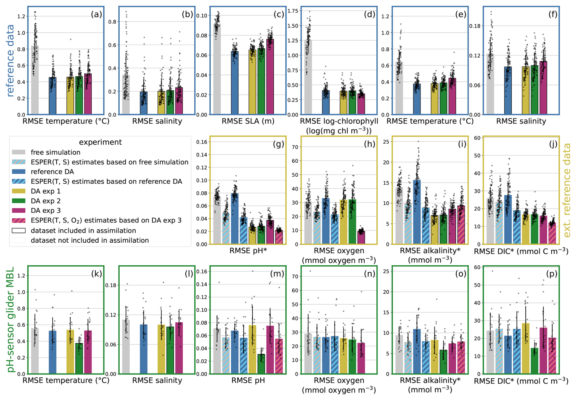
Figure 4 RMSE for the main experiments: Each panel corresponds to a dataset (displayed in Fig. 2 in the same panel layout), the bars represent model experiments: small black dots display the RMSE of a simulation for that dataset, for each cycle which includes data for the dataset. The height of the bar displays the average cycle RMSE, and the black line on each bar shows the mean ± standard deviation of the cycle RMSE. Black outlines of bars indicate that the dataset was assimilated in the experiment.

We first examine the root mean squared error (RMSE) between model and data for each dataset introduced in Sect. 2.3. Comparing the two experiments reveals that, similar to previous studies jointly assimilating chlorophyll and physical data (e.g. Mattern et al., 2017), the DA substantially improves the fit to the assimilated data compared to the free simulation (compare gray and blue bars in Fig. 4). However, this reduction in error for physical and chlorophyll data (first row in Fig. 4) does not translate to improved fit for glider observations of carbonate system variables (pH, alkalinity, DIC) or oxygen (second row in Fig. 4). Notably, there is no improvement in the reference DA experiment even though it assimilates temperature and salinity data from the same CUGN glider lines associated with the carbonate system variables.

A closer examination of a representative glider line reveals the spatial structure of the model-observation differences for pH. We focus on a CUGN Line 67 glider transect out of Monterey Bay (see highlighted line in Fig. 2g) starting in late March 2019, which we refer to as CUGN L67Mar (Fig. 5). The discrepancies between pH observations and free simulation model estimates along this line are highest between 50 and 200 m depth (Fig. 5d, e, f), corresponding to density surfaces of 1025.5–1027 kg m⁻³. Near the surface and at depths below 300 m, the free simulation shows a positive bias, overestimating pH by ≈ 0.1. Assimilation of the reference data, including temperature and salinity data from this line, does not remove the surface or deep pH bias, and results in minor shifts in the largest model-observations differences at intermediate depths between 50 and 200 m (compare Fig. 5f and h). The improvement in pH estimates, measured by the reduction in the absolute model-observation difference of the reference DA in comparison to the free simulation (Fig. 5i) confirms that the largest change in model pH through the assimilation of the reference data occurs in the same depth range (50 to 200 m), where the reference DA leads to positive and negative changes in pH estimates.

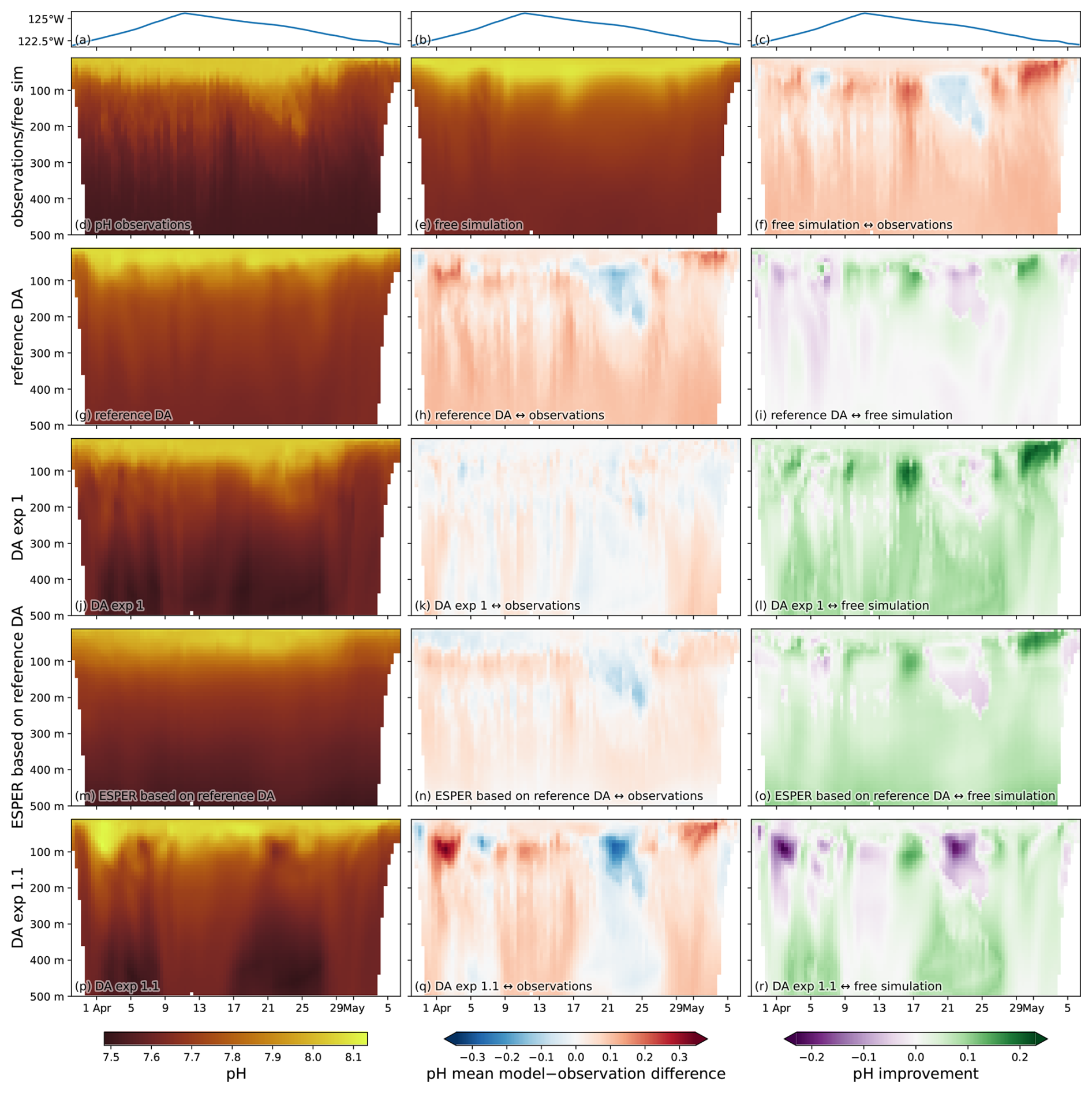
Figure 5 Glider pH transect for CUGN L67Mar: The glider-based pH observations and model pH estimates at the observation locations for a glider transect along Line 67 started in late March 2019. (a–c) The longitude of the glider, indicating its position along the east-west line for each date. (d) Glider pH observations binned on a date-depth grid focused on the top 500 m. The model pH estimates on the same grid for the (e) free simulation, (g) reference DA, (j) DA exp 1, (m) hybrid estimate using ESPER based on the reference DA, and (p) DA exp 1.1. (f, h, k, n, q) The model-observation difference for pH along the transect for all 5 pH estimates. (i, l, o, r) The improvement of the estimates in comparison to the free simulation (the absolute value of the model-observation difference for the free simulation minus the absolute value of the model-observation difference for the DA-based or hybrid estimate). Positive (green) values indicate a reduction in model misfit of the DA-based or hybrid estimate in comparison to the free simulation.

In our state estimation setup, the joint assimilation of temperature, salinity, SLA, and chlorophyll data has negligible impact on estimates of pH, oxygen, alkalinity, or DIC. This finding aligns with previous state estimation studies reporting little impact of physical DA on chlorophyll estimates, which we will discuss further in Sect. 4.

3.2 Assimilating pH and alkalinity data

Because the joint physical and chlorophyll DA showed no consistent improvements in pH estimates, we next examine the simulation that assimilates CUGN-based pH and alkalinity estimates in addition to the reference data, in the experiment referred to as “DA exp 1”. The joint assimilation of pH and alkalinity estimates with physical and chlorophyll data leads to significant improvement in the model carbonate chemistry parameters. DA exp 1 more than halves the average RMSE of the CUGN pH data compared to the free simulation or the reference DA, while achieving a similar fit to the reference data temperature, salinity, SLA and chlorophyll as the reference DA (Fig. 4). The improvement in pH is accompanied by improved fit to CUGN alkalinity and DIC data (Fig. 4i, j), with little change in oxygen estimates (Fig. 4h).

Examining the CUGN L67Mar transect (Fig. 5j–l), the assimilation of pH data leads to overall improvement in pH estimates: surface and deep biases shown in the reference DA are removed, and larger pH discrepancies at intermediate depths disappear.

In the results above, we have only examined the fit to data that has been assimilated. To better understand the spatial influence of pH DA, we examine the increments in DA exp 1 to the carbonate system variables. When only assimilating physical and chlorophyll data, the DA system does not create corrective increments to the carbonate system variables (as these have no direct influence on the physical or chlorophyll state estimates; compare Fig. 1). That is, in the reference DA, the carbonate system variables are only affected indirectly by the DA through increments in the physical and nitrogen-based variables and subsequent changes in physical and biogeochemical model dynamics. In DA exp 1, however, the assimilation creates significant increments to alkalinity and DIC to improve the fit to the CUGN pH and alkalinity observations.

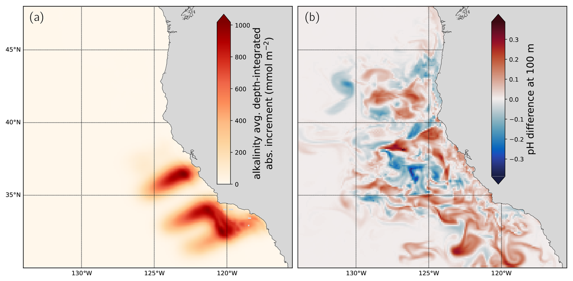
Figure 6 Impact of the pH DA: (a) The average depth-integrated absolute increment in alkalinity across all 91 DA cycles in DA exp 1. (b) The difference in pH between the reference DA (not assimilating pH data) and DA exp 1 at 100 m depth at the end of the 91 DA cycles on 31 December 2019.

The average depth-integrated absolute alkalinity increment (Fig. 6a) illustrates the horizontal extent of influence of the pH assimilation, clearly outlining the 2019 CUGN glider lines that were assimilated (compare Fig. 2g, i). Each increment represents the difference between the model state before and after DA at the start of each cycle, which is influenced by the 50 km horizontal length scale prescribed in the DA setup. Thus, it does not capture the subsequent effect of DA due to the model dynamics (the cumulative effect of the increments on the physical and biogeochemical model dynamics through each cycle).

To assess the downstream effect of pH assimilation, we examine the difference in pH estimates at 100 m depth between DA exp 1 and the reference DA at the end of the experiments (31 December 2019). After a full year of assimilating data, the pH difference at 100 m depth has spread from the pH observation locations along the coast and offshore (Fig. 6b). The snapshot of pH difference reveals complex structures, with areas of positive pH change bordering water masses with negative change. In Sect. 3.4 and 3.5, we examine if the pH DA improves the fit to pH data that has not been assimilated.

3.3 Hybrid estimates based on ESPER

Hybrid estimates use the output of the dynamical model as input to the statistical ESPER model (see Sect. 2.4). As DA can lead to substantial improvements in dynamical model estimates, it is likely to produce better hybrid estimates.

Because the temperature and salinity model estimates do not appear to benefit from the assimilation of carbonate system data (Fig. 4e, f), we only produce ESPER estimates based on the output of the free simulation and the reference DA. We do not use model oxygen as inputs for the ESPER estimates because model initial conditions for oxygen are based on ESPER estimates and DA experiments have shown little improvement in oxygen estimates compared to the free simulation (compare Fig. 4h). Instead, here we use ESPER based on temperature and salinity only, and examine the assimilation of oxygen data and ESPER estimates based on assimilated temperature, salinity, and oxygen in Sect. 3.6.

Using model temperature and salinity, we generate ESPER-based estimates throughout the entire model domain. Here, we focus on ESPER estimates of pH, alkalinity, and DIC at the observation locations, that is, at the time and place glider observations were recorded. Comparing these values to the CUGN data reveals that hybrid estimates have a better fit than model-based estimates for pH, alkalinity, and DIC (Fig. 4g, i, j), except for DA exp 1, 2, 3 which all directly assimilate CUGN pH and alkalinity data. For oxygen, hybrid estimates create the closest fit to CUGN observations among all estimates considered so far. In all cases, ESPER estimates based on the reference DA outperform those based on the free simulation, benefiting from improved temperature and salinity estimates obtained through physical DA.

The hybrid pH estimates for ESPER based on the reference DA along CUGN L67Mar (Fig. 5m–o), show a reduced misfit to data compared to the free simulation and reference DA. The largest misfit occurs at depths around 100 m, corresponding to the 1026 kg m⁻³ density surface.

In summary, hybrid estimates based on model temperature and salinity, combined with the ESPER statistical model, produce some of the best carbonate system estimates in our study, unless the carbonate system data itself is assimilated. Notably, these hybrid estimates do not require a biogeochemical ocean model and can be obtained from a physical ocean model and physical DA, an aspect we examine in more detail in Sect. 4.

3.4 Evaluation using independent Line 67 data

In previous sections, we examined model-based and hybrid estimates for data that was assimilated in some experiments and where pH and alkalinity were not directly measured but estimated using a statistical model. Here, we evaluate the same estimates against a new glider-based dataset that is not part of the CUGN data, contains direct pH measurements along with temperature, salinity, and oxygen, and was not assimilated in the experiments introduced so far. This dataset, referred to as the pH-sensor glider line data, was recorded during several MBARI glider deployments. These deployments spatially overlap with the CUGN Line 67 (see Fig. 2) and are thus in the region strongly influenced by the CUGN pH DA (see Fig. 6).

For comparison with the pH-sensor glider line data, we introduce an additional experiment, DA exp 2, which assimilates pH-sensor glider line temperature, salinity, pH, and alkalinity data, as well as reference data and CUGN pH and alkalinity data. DA exp 2 serves two main functions: to determine the estimates for the pH-sensor glider line achievable through direct assimilation and to demonstrate that CUGN pH data and measured pH-sensor glider line pH data can be jointly assimilated without deteriorating estimates for either dataset. To run DA exp 2, we rely on statistical estimates of alkalinity for the pH-sensor glider line, jointly assimilated with measured pH data, and include estimates of DIC by combining measured pH and estimated alkalinity (which has a lower error relative to DIC estimated directly from algorithms) in the pH-sensor glider line data for comparison.

We first examine the 4 d RMSE values of model and hybrid estimates with respect to the pH-sensor glider line data (Fig. 4k–p). For temperature and salinity, DA experiments perform similarly to the free simulation, with only DA exp 2 showing improvement. Assimilation of large temperature and salinity datasets, including CUGN data, does little to improve overall estimates at the pH-sensor glider line.

These results from physical data also apply to the carbonate system variables. For pH, DA exp 1 performs slightly worse on average than the reference DA and free simulation, with only hybrid estimates and direct assimilation (DA exp 2) performing better. Results for alkalinity and DIC are similar to pH; for oxygen, all estimates perform comparably, and DA-based estimates only slightly outperform the free simulation.

For pH, the largest misfit between model estimates and pH-sensor glider line observations occurs near the surface and at intermediate depths down to 150 m, with no deep pH bias for simulations assimilating CUGN pH data (not shown). The structure of pH differences between estimates from the reference DA and DA exp 1 (Fig. 6b) provides context for why the DA cannot substantially improve intermediate depth estimates along glider Line 67 extending out of Monterey Bay. The region is highly active in terms of physical circulation and DA impact, with large pH changes occurring on relatively small spatial scales. We conclude that our DA requires spatially or temporally denser observations to inform the model about the evolving pH field, and only the direct assimilation of pH-sensor glider line pH observations significantly reduces pH misfit in the top 150 m.

3.5 Cross-validation experiments

To better understand model pH estimates for non-assimilated data, we performed three additional cross-validation experiments. In these experiments, different subsets of CUGN pH and alkalinity data were withheld from assimilation. We focus on the Line 67, and three glider transects in different seasons: CUGN L67Mar, CUGN L67Jul, and CUGN L67Oct (CUGN L67Mar is used in Fig. 5). For each line, we created an experiment that assimilates all data from DA exp 1 (reference data and CUGN pH, alkalinity), except for the CUGN temperature, salinity, pH, and alkalinity data associated with that specific transect. These three new experiments are denoted DA exp 1.1, 1.2, and 1.3 (see Table 2).

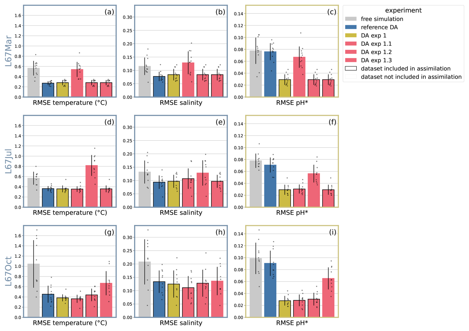
Figure 7 RMSE in cross-validation experiments: RMSE quantifying the model-observation misfit for the three CUGN deployments along Line 67, subsets of the CUGN data, used in the cross-validation experiments in Sect. 3.5. Each panel represents a dataset, the bars represent model experiments: small black dots display the RMSE of a simulation for that dataset, for each cycle which includes data for the dataset. The height of the bar displays the average cycle RMSE, the black line on each bar shows mean ± standard deviation of the cycle RMSE. Black outlines of bars indicate that the dataset was assimilated in the experiment. The cross-validation experiments DA exp 1.1, 1.2, and 1.3 withheld CUGN L67Mar, L67Jul, and L67Oct, respectively.

We examine the RMSE of DA exp 1.1, 1.2, 1.3 in comparison to DA exp 1, the reference DA, and free simulation for the three datasets (Fig. 7). In some cases, such as CUGN L67Mar salinity (Fig. 7b), the error of DA exp 1.1 is highest and even exceeds that of the free simulation. This suggests that in some cases, the advection of increments may cause model-data discrepancies downstream, likely due to the filamentous structure of the change in pH after less than a year of carbonate system DA (Fig. 6b). However, for most datasets, the cross-validation experiments perform better than no assimilation of CUGN data. A clear example is the pH RMSE for CUGN L67Mar (Fig. 7c), where the free simulation and reference DA show the highest error (both not assimilating CUGN pH data), while the experiments assimilating CUGN L67Mar data (DA exp 1, 1.2, and 1.3) have the lowest error values. The cross-validation experiment DA exp 1.1 is in between the two results, and benefits from the assimilation of the surrounding CUGN data.

A closer look at pH estimates from cross-validation experiment DA exp 1.1 along CUGN L67Mar reveals that assimilation of neighboring CUGN data positively affects deep pH, largely removing the positive bias seen in free simulation and reference DA (Fig. 5p–r). However, small patches of high model-data misfit at intermediate depths (≈ 100 m) indicate that advection of pH increments from other parts of the CUGN line can cause local increases in error.

In summary, the cross-validation experiments demonstrate that glider DA of pH data typically positively affects pH estimates near the observation network, but advection of assimilative increments can negatively affect downstream estimates. We examine this interesting point further in Sect. 4.

3.6 Assimilation of oxygen data

Changes in pH and dissolved oxygen are closely related because both are affected by important biogeochemical processes such as primary production, plankton respiration, and the decomposition of organic matter. These pathways are included in the NEMUCSC model; however, despite this connection, the assimilation of pH data leads only to minor changes in oxygen in our previous experiments (Fig. 4h, n). Two main factors in the setup of our assimilation system contribute to this limited impact: (1) The ROMS DA system sets covariance terms between different variables to zero. (2) Our DA configuration favors corrections to observed variables (such as alkalinity) over corrections to unobserved variables (such as the nutrient variables). Thus, the assimilation of pH data mainly modifies model alkalinity and DIC and because changes in these two variables do not directly affect oxygen, the effect of pH DA on oxygen is low. We discuss these factors in more detail in Sect. 4.

To address this limitation, our final set of experiments includes oxygen observations in the assimilation. DA exp 3 assimilates the reference data along with CUGN pH, alkalinity, and oxygen (Table 2). This additional assimilation of oxygen leads to marked improvement in oxygen estimates for the CUGN data compared to DA exp 1 (Fig. 4h). It also results in a minor increase in error for most other assimilated variables (Fig. 4a–g, i). This increase is consistent with the inclusion of more observations in the DA, which downweights other observations in the 4D-Var state estimation procedure. Importantly, this result does not imply that a better fit to oxygen observations necessarily creates worse estimates for temperature or other variables.

Notably, DA exp 3 creates better oxygen estimates than the hybrid ESPER-based estimates. This effect mirrors the results for pH estimates, where direct assimilation in DA exp 1 outperformed the hybrid estimates based on temperature and salinity. Building on the improved oxygen estimates from DA exp 3, we create an additional hybrid estimate. This new estimate is based on DA exp 3 and ESPER, including oxygen as an input to ESPER alongside temperature and salinity. The resulting hybrid model produces the best pH estimates and generally outperforms the previously introduced hybrid models, which are based on temperature and salinity alone.

In summary, the addition of dissolved oxygen observations in the assimilation yields improved oxygen estimates without a substantial negative effect on other observed variables. Furthermore, the inclusion of assimilated oxygen in hybrid estimates improves their performance compared to those based on temperature and salinity alone. However, it is important to note that this approach requires a DA system that includes a biogeochemical model with oxygen.

4 Discussion

Our study pursued three main goals related to improving carbonate system and oxygen state estimates through data assimilation. First, we examined the effect of the joint assimilation of carbonate system variables and oxygen data with physical and chlorophyll observations that are traditionally assimilated. As a baseline we used the reference DA experiment which only assimilates observations of temperature, salinity, sea level anomaly, and chlorophyll. This reference DA experiment significantly improves the fit to the assimilated variables but has a very limited impact on model estimates of pH and oxygen. In contrast, the joint assimilation including pH, alkalinity and oxygen observations successfully improves estimates of these variables while largely maintaining the quality of physical and chlorophyll estimates. This effect is likely due to a down-weighting of the reference observations – consisting of satellite-, float-, and glider-based temperature, salinity, sea level anomaly, and chlorophyll – in the 4D-Var state estimation procedure simply due to the presence of more observations.

Second, we investigated how the assimilation of different data subsets influences the model state estimates. In our configuration, the traditional physical-chlorophyll DA, represented by our reference DA experiment, has minimal impact on pH and oxygen estimates, even when assimilating temperature and salinity data from the same observation platforms that measured pH and oxygen. Similarly, pH DA shows limited influence on oxygen estimates. This limited impact across variables likely stems from two key factors in our DA implementation: (1) the ROMS 4d-Var DA system presently allows for univariate covariances only (i.e., with zero covariance between different variables and with no ability to specify non-zero cross-variable covariance values), and (2) our configuration, in particular the background error specification (see Sect. 2.5), favors increments to directly observed variables over unobserved ones. As a result, our current DA setup allows larger increments to alkalinity and oxygen directly but not to unobserved variables that have pathways with feedback to these variables, such as nitrate, a main driver of primary production that modifies both oxygen and pH. This inherent limitation of our DA system could mean that alternative techniques, such as ensemble-based DA, which automatically include cross-variable covariances, could create larger improvements in unobserved variables from the assimilation of pH data.

Third, we evaluated whether combining output from the dynamical ROMS model with the statistical ESPER model can produce improved carbonate system state estimates without the need for a biogeochemical model. Our results show that these hybrid estimates based on ESPER using only ROMS temperature and salinity as inputs often produce better results for pH, alkalinity, DIC, and oxygen than the biogeochemical model without assimilating carbonate system variables or oxygen. Importantly, the hybrid estimates benefit from physical DA through improved temperature and salinity estimates and do not require a biogeochemical model. This result suggests that existing physical ocean models and physical DA systems can be used to obtain good carbonate system estimates without implementing complex biogeochemical models if the statistical model estimates are reliable.

A practical constraint in our pH DA implementation is the requirement for joint assimilation with alkalinity data (see Sect. 2.6). Since total alkalinity is not routinely measured by autonomous platforms, the assimilation relies on statistical estimates. This dependence on estimated alkalinity data represents a potential limitation of our approach in cases when the alkalinity estimates may not be accurate. For example, this DA approach has limited use in cases where the alkalinity has been altered (e.g., as part of a marine carbon dioxide removal (mCDR) experiment (Boyd et al., 2023; Fennel et al., 2023)). Other instances of unreliable estimates from global algorithms like ESPER may include regions near river mouths with significant organic matter input from terrestrial sources or following large denitrification events at the end of a seasonal phytoplankton bloom or in anoxic basins. In these latter cases, regional statistical models, specifically trained for their area of interest, may be able to produce more accurate local estimates. If there has been no alteration and statistical estimates of alkalinity are reliable, our results suggest that the statistical estimates are sufficiently accurate for effective pH state estimation.

In this study, we are using super-observations for assimilation while employing the original, non-aggregated observations for visualization and error metrics. This approach proves particularly beneficial for dense glider observations, where multiple measurements often occur within the same model grid cell and time step. Using the original observations for RMSE calculations (Figs. 4, 7) provides a more stringent test of model performance and better represents the true observational density in our visualizations. Interestingly, the model experiments often show a better fit to the original observations than to super-observations. The improved fit is due to the structure of the model grid and vertical differences in the model-observation misfit: the model has terrain-following coordinates, with a higher resolution near the surface, so that deeper grid cells are larger. As a result, on average, fewer original observations are combined into super-observations near the surface, shifting the proportion of observations upward. Because the model estimates typically have a higher error near the surface, the increased proportion of near-surface super-observations creates a higher mean error when using super-observations.

The use of statistical models for both data generation and estimation in our study warrants careful consideration. In our current setup, we assimilate algorithm-based pH and alkalinity data for the CUGN lines, as well as algorithm-based alkalinity for the pH-sensor glider line. Simultaneously, we use ESPER for our hybrid estimates, creating a relationship between data and the hybrid estimates. For the hybrid estimates using the reference run, we only used temperature and salinity as inputs for ESPER, whereas the CUGN estimates are based on an average of three statistical algorithms, with temperature, salinity, and oxygen as inputs. Yet we use temperature, salinity, and oxygen for the hybrid estimates for DA exp 3, creating a closer relationship between the validation data and the hybrid estimates. Hence, the good fit of the hybrid estimates to pH data (see Fig. 4g) is less a result of the quality of the ESPER estimates and more a result of the DA system's ability to move model estimates closer to the glider observations. However, validation experiments (Fig. 3) show that the algorithm used to generate the data provides reliable estimates of alkalinity, DIC, and pH across the model domain. Furthermore, hybrid estimates also show a good fit to measured pH data in our experiments (Fig. 4m) and even the ESPER estimates based on the free simulation (and only temperature and salinity input) outperform pH model estimates from simulations that did not assimilate pH data. Hence, dependent on the setup and scope of the study, we consider hybrid estimates as valid alternatives to complex biogeochemical models.

Looking ahead, several important challenges emerge from this study that warrant further investigation. The temporal scope of our analysis, limited to 2019, leaves open questions about the long-term effectiveness of the DA system. Here, we are planning to extend the DA beyond 2019, complemented by validation against data not included in the DA system, for example, from the BGC-Argo program (Claustre et al., 2020) and recent high-resolution pCO₂ products for the CCS (Sharp et al., 2022). We further aim to address current methodological limitations through modification of background and observation error values in the 4D-Var system using the methodology presented in Mattern et al. (2018). For this purpose, we require statistics computed from completed 4d-Var DA experiments, and the experiments presented in this study could form the basis for improved background and observation error specifications, especially for the carbonate system variables and oxygen in our DA system. Such an approach requires additional research because model pH is a diagnostic variable, and pH observation error values will need to be balanced with alkalinity and DIC background error values. We may further investigate the implementation of ensemble-based DA (e.g., using the framework presented in Mattern and Edwards, 2023) to better account for cross-variable covariances.

By demonstrating the feasibility of joint DA of physical, chlorophyll, and carbonate system variables and hybrid estimation approaches, this study provides practical pathways for improving carbonate system state estimates in dynamic coastal environments. These methodological advances support broader efforts to quantify regional carbon budgets and air-sea CO₂ exchange, contributing to our understanding of how coastal systems respond to and influence global carbon cycling. The framework developed here is particularly relevant as ocean observing systems expand and the need for accurate coastal carbon cycle monitoring grows more urgent in the face of climate change and ocean-based mitigation efforts like mCDR.

5 Conclusions

In this study, we examined the effects of integrating glider-based pH, alkalinity, and oxygen data into a joint physical-biogeochemical DA system. In our reference DA configuration, the assimilation of physical and chlorophyll data has little effect on the model state estimates for pH or oxygen. However, the joint assimilation of pH, alkalinity, and oxygen data substantially improves carbonate system estimates without degrading the quality of physical and chlorophyll estimates. For carbonate system DA, our approach relies on assimilating observed pH jointly with statistically estimated alkalinity data which succeeds in our application but may lead to issues in scenarios where alkalinity estimates are unreliable. Cross-validation experiments show that pH data assimilation typically improves estimates near the observation network, although downstream advection of increments can occasionally degrade results. A hybrid approach, which combines the output of the dynamical ROMS model with ESPER statistical estimates of pH and oxygen, produces good carbonate system estimates that benefit from physical data assimilation while eliminating the need for a biogeochemical model. While this study is limited to 2019, it is the basis for extending the DA to the following years and examining the continued impact on the carbonate system and ocean acidification state estimates in a highly dynamic coastal ecosystem.