A machine learning approach to driver attribution of dissolved organic matter dynamics in two contrasting freshwater systems

Predicting water quality variables in lakes is critical for effective ecosystem management under climatic and human pressures. Dissolved organic matter (DOM) serves as an energy source for aquatic ecosystems and plays a key role in their biogeochemical cycles. However, predicting DOM is challenging due to complex interactions between multiple potential drivers in the aquatic environment and its surrounding terrestrial landscape. This study establishes an open and scalable workflow to identify potential drivers and predict fluorescent DOM (fDOM) in the surface layer of lakes by exploring the use of supervised machine learning models, including random forest, boosting methods, k-nearest neighbors, support vector regression and linear model. The workflow was validated in two contrasting systems: one natural lake in Ireland with a relatively undisturbed catchment, and one reservoir in Spain with a more human-influenced catchment. A total of 24 potential drivers were obtained from global reanalysis data, and lake and river process-based modelling. SHapley Additive exPlanations (SHAP) were conducted for the most influential drivers identified, with soil moisture, soil temperature, and Julian day being common to both study sites. The best prediction was obtained when using the CatBoost model (during hold-out testing period, Irish site: KGE > 0.68, r²>0.50; Spanish site: KGE > 0.66, r²>0.54). Interestingly, when only using drivers from globally accessible climate and soil reanalysis data plus Julian day, the prediction capacity was maintained at both sites, showcasing potential for scalability. Our findings highlight the complex interplay of environmental drivers and processes that govern DOM dynamics in lakes, and contribute to the modelling of carbon cycling in aquatic ecosystems.

1 Introduction

Lakes are an essential component of global biogeochemical cycles, sustain biodiversity, and provide critical ecosystem services, e.g., water supply, fishing and irrigation. However, their water quality is increasingly at risk due to climatic change and human pressures (Bhateria and Jain, 2016). A key water quality variable is dissolved organic matter (DOM), which influences light penetration, energy, oxygen dynamics and nutrient availability in any lake (Solomon et al., 2015). The dynamics of DOM in lakes are driven by both external processes in the terrestrial environment and internal processes. Land cover, climate, and topography regulate (either increase or decrease) carbon production in the catchment and carbon inputs into the lake (Li et al., 2015). In the water body, the quantity and quality of DOM are controlled by physical and biogeochemical mechanisms such as photodegradation, microbial processing and mixing dynamics, but can also be impacted by water abstraction or dam regulation (Xenopoulos et al., 2021).

Increases in the concentrations of DOM can affect ecosystem stability and human water use (e.g., raw drinking water quality) by reducing oxygen levels, altering microbial communities and nutrient cycling (Lake et al., 2000). DOM is also a precursor to disinfection byproducts (DBPs) during drinking water treatment, substances which have negative human health implications (Li et al., 2014). Understanding the dynamics of DOM in lakes is essential for water quality management, especially as climate-driven processes are expected to increasingly influence DOM in freshwater systems (Creed et al., 2018). Moreover, the occurrence of extreme events such as eutrophication, algal blooms and hypoxic events, for which levels of DOM play a key role, is also expected to increase (Gobler, 2020). Hence, predicting DOM in lake water can improve water quality mitigation protocols and support adaptive water use management strategies.

Predicting DOM dynamics remains a challenge as it results from complex interactions in the environment, including multiple biogeochemical processes (Weyhenmeyer and Karlsson, 2009). Modelling tools offer an approach to simulate DOM in lake water. Process-based models have traditionally been used to better understand lake water quality, including DOM dynamics (McCullough et al., 2018). However, they generally require a large number of model parameters and governing equations, i.e., extensive parameterisation, to represent these dynamics. On the other hand, machine learning (ML) models do not rely on parameter calibration but instead incorporate large amounts of driver variables and data. This functionality can leverage the increasing amount of data being collected through satellite imagery, high frequency monitoring, and global climate and environmental modelling initiatives (Müller et al., 2024; Toming et al., 2020; Asadollah et al., 2025).

ML models have emerged as potential tools for modelling complex environmental variables, including those related to hydrology (Nearing et al., 2021) and water quality (Hanson et al., 2020). They have been recently employed in environmental applications, showing good predictive capabilities due to their ability to handle high-dimensional data, and capture nonlinear relationships (Li et al., 2016), for a diversity of parameters in lakes such as chlorophyll-a (Chen et al., 2024), turbidity (Zhang et al., 2021), and nutrient concentrations (e.g., phosphorus) (Hanson et al., 2020), suggesting potential for predicting DOM (Herzsprung et al., 2020).

This study introduces a workflow for predicting fluorescent DOM (fDOM) (a proxy for DOM) in lakes using a suite of supervised ML models driven by potential drivers either extracted from reanalysis data (climate and soil variables) or outputs from lake and catchment process-based models. The workflow was tested in two different study sites, one in Ireland and one in Spain, that represent contrasting settings for both the potential drivers and DOM dynamics. Model performance was first evaluated at each site using the most influential drivers to predict fDOM. Subsequently, a second simulation was performed using a subset of these drivers, limited to those sourced from reanalysis data, to evaluate the predictive capacity of the model in the context of higher scalability. A primary intention of the study is to use ML models to produce a robust, accessible, and reproducible workflow, rather than to conduct an extensive model benchmark comparison. The aims of this study are: (1) to find the most influential drivers (features) in predicting fDOM, and analyse their importance in two contrasting sites; (2) to test how accurately can supervised ML models predict lake fDOM driven by reanalysis-based data, and hydrologic and lake modeling outputs.

2 Materials and methods

2.1 Study sites

Lough Feeagh and Sau Reservoir are located in western Ireland (53°56^′ N, 9°35^′ W) and northeastern Spain (41°58^′ N, 2°23^′ E), respectively (Fig. 1). The study sites have contrasting attributes. Feeagh (depth of 46.8 m and area of 3.95 km²) is a monomictic and oligotrophic lake surrounded by a relatively undisturbed landscape, while Sau (depth of 70 m and area of 5.8 km²) is an eutrophic system subjected to human activities and water abstraction. Feeagh has two primary inflows, the Black and the Glenamong rivers, while Sau has one, the Ter river. The catchment of Feeagh is relatively small (84 km²), with mid-range hills, and dominated by peatland. The catchment of Sau, in contrast, is larger (1525 km²), with a varying topography and land uses (Figs. 1, A1).

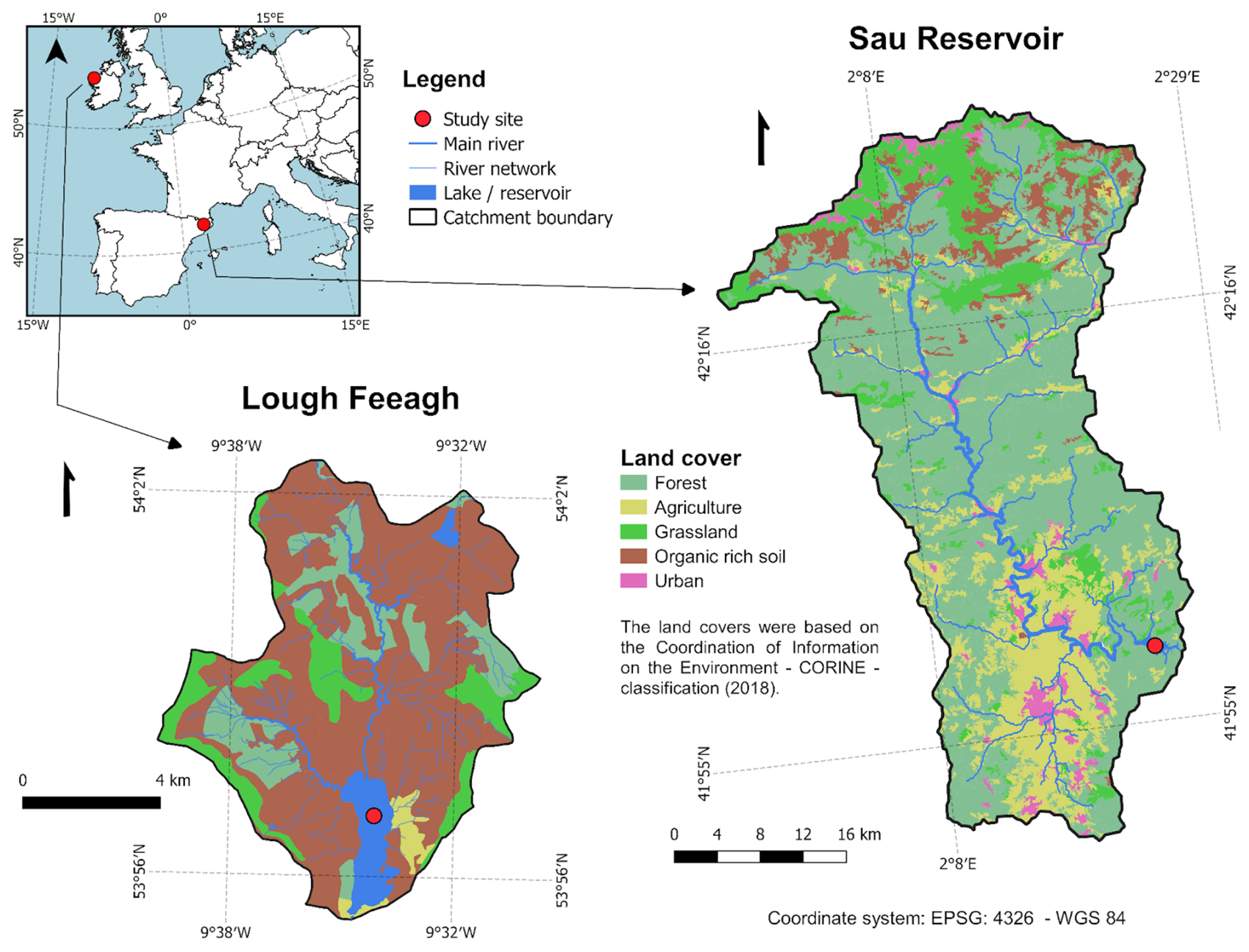
Figure 1 Two contrasting freshwater ecosystems: Lough Feeagh (Ireland) and Sau Reservoir (Spain). The figure shows their locations and catchment land cover. Lough Feeagh is a humic oligotrophic lake with a peatland-dominated catchment and temperate oceanic climate, whereas Sau is a eutrophic reservoir with a human-influenced catchment and Mediterranean climate. The CORINE Land Cover 2018 https://doi.org/10.2909/960998c1-1870-4e82-8051-6485205ebbac (EEA, 2020) classes were grouped into the categories shown for visual clarity, following the aggregation approach described in the Appendix (Fig. A2).

The dynamics of DOM in both study sites have been previously explored in Ryder et al. (2014) which identified that natural dynamics related to soil temperature, river discharge and drought were important drivers in Feeagh, and in Marcé et al. (2021), which showed human activities (e.g., wastewater effluents and agricultural runoff) were important for Sau, in addition to its environmental dynamics. Catchment hydrology is key for carbon transport into both study sites, and contributes to a distinct seasonality related to climate. Feeagh has a wet temperate climate, with cooler air temperatures and higher rainfall levels that occur on more than 75 % of days in the year. The variability of carbon inputs reflects the sensitivity of a peatland-dominated landscape, which exacerbates climate-induced carbon release from the catchment into the lake. In contrast, Sau has a Mediterranean climate, characterised by hot, dry summers and mild, wet winters, dictating water availability, thermal stratification, and organic matter fluxes in the reservoir.

2.2 Prediction workflow

A five-step workflow was implemented to predict fDOM at each site (Fig. 2). First, all potential drivers for fDOM were collected as input data for each site. Second, an exploratory data analysis of fDOM was implemented and the ML models were trained using 85 % of the available time series data (1978 out of 2328 fDOM measurements for Feeagh, and 653 out of 769 for Sau), while the remaining 15 % (350 out of 2328 for Feeagh, and 116 out of 769 for Sau) future time series (hold-out period) was reserved for independent testing to evaluate performance and potential overfitting by comparing with the training period.

Third, a set of drivers was selected for each site based on the variable importance extracted from the ML models, retaining only those drivers that exceeded an importance threshold of 5 %. SHAP and partial dependence analyses were applied to these specific drivers to evaluate how fDOM predictions at each site varied as a function of individually changing the selected input variables. Fourth, we ran simulations using (i) the drivers with a higher variable importance (> 5 %), and (ii) using only drivers extracted from globally accessible reanalysis data, and assessed model.

The same workflow was applied to both sites using the same data sources, allowing for comparison. Following the FAIR principles, all data and workflow scripts are available and fully reproducible here: https://doi.org/10.5281/zenodo.19354955 (Mercado-Bettín, 2026). Large language models were used in this study to optimise the codes, improve the final plots and, for basic proofreading of the text.

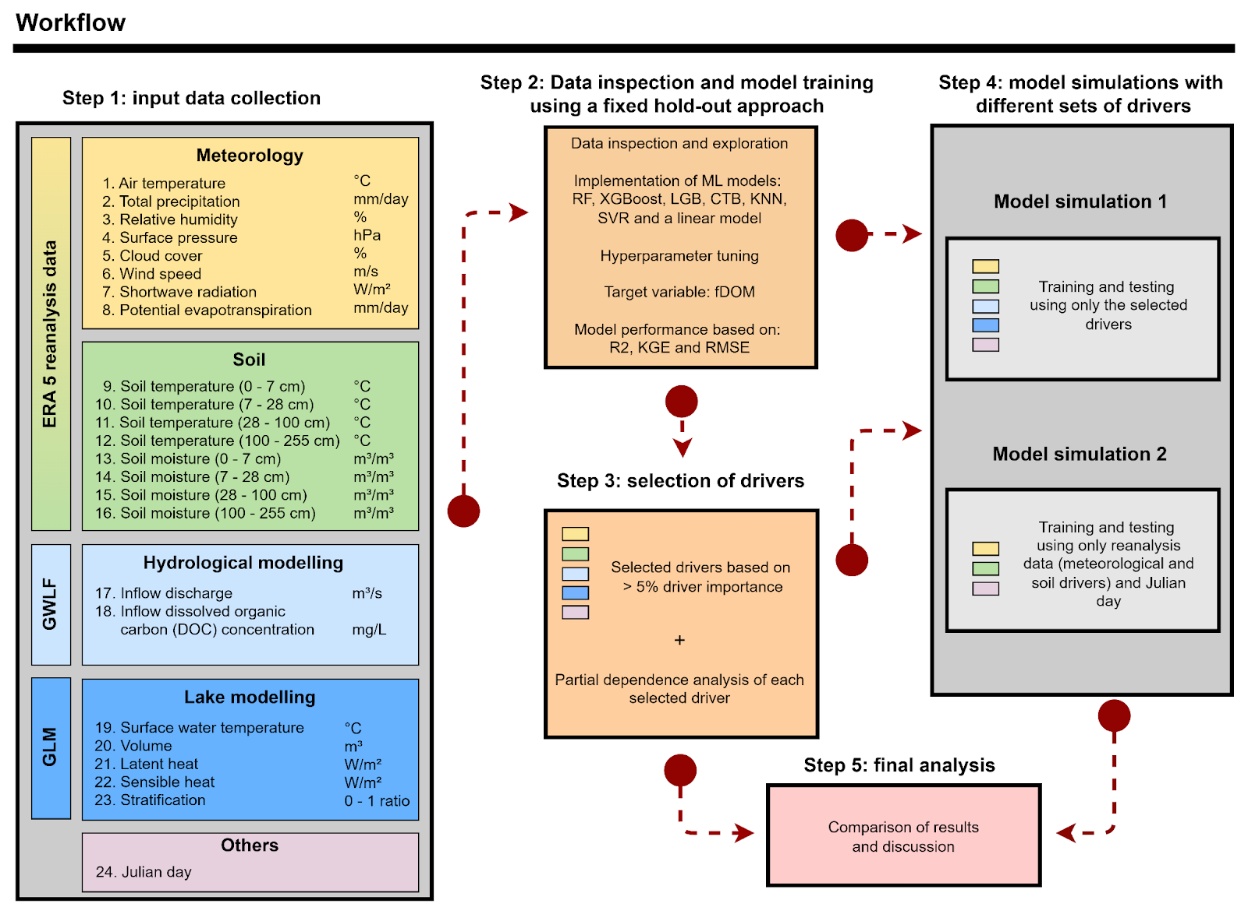
Figure 2 The workflow includes five steps: (1) compilation of input variables including meteorology (yellow) and soil (green) reanalysis data from ERA5 (the fifth-generation atmospheric reanalysis product produced by ECMWF), The Generalised Watershed Loading Functions Model (GWLF) outputs (light blue), The General Lake Model (GLM) outputs (blue), and Julian day (light magenta); (2) data inspection and model training using a split between training (85 %) and testing (15 %) periods; (3) selection of influential drivers based on feature-importance metrics; (4) model simulations using selected drivers and a reduced subset based on globally available reanalysis variables and Julian day; and (5) comparison of model outputs. DOC stands for Dissolved Organic Carbon. The workflow is available at: https://doi.org/10.5281/zenodo.19354955 (Mercado-Bettín, 2026).

2.3 Data

2.3.1 Target variable (fDOM)

Daily surface fDOM values were obtained from high-frequency data for both sites (2 min-resolution data averaged to obtain daily values before analysis). For Feeagh, data were measured at 0.9 m depth, and for Sau, an average value was calculated between the measurements for depths 0–5 m. fDOM data were expressed as quinine sulfate units (QSU) for the analysis. In Feeagh, the data spanned from 1 May 2012 to 19 November 2019 (n=2328), and for Sau from 4 February 2017 to 2 March 2020 (n=769), with some gaps. All the other data (i.e., driver data) used in the workflow of this study were constrained by the availability of fDOM data. Following exploratory data analysis (Fig. A3), no transformation was applied to the fDOM data prior to training the ML models in the main manuscript, results for Sau are provided with a log₁₀ transformation in the Appendix for comparison (this is revisited in Results), given the moderate skewness of fDOM at this study site.

In Feeagh, fDOM data were collected using a Seapoint UV fluorometer sensor (Seapoint Sensors Inc., Exeter, NH, USA) and water temperature data were measured using a Hach Environmental Hydrolab Data Sonde X5 (UK OTT Hydrometry Ltd). In Sau, fDOM and water temperature data were collected using a fDOM Digital Smart Sensor and Multiparameter Sonde (YSI EXO sonde, Yellow Springs, OH, USA), respectively. Raw fDOM data were water temperature-corrected in both sites based on relationships established for each sensor (Ryder et al., 2012). Details about the fDOM corrections can be found in the Appendix (Figs. A4, A5 and A6).

2.3.2 Driver data

All input data variables, including their respective units and source, are displayed in Step 1 of Fig. 2. These were grouped into five categories: (1) meteorology, (2) soil, (3) process-based hydrological modelling, (4) process-based lake modelling and (5) Julian day. All input data variables, including their respective units and source, are displayed in Step 1 of Fig. 2. Daily values of meteorology and soil variables were extracted from the European Centre for Medium-Range Weather Forecasts (ECMWF) Reanalysis v5 (ERA5) dataset (, ). This gridded dataset provides (pseudo) observations at a global scale with a spatial resolution of 0.25°. Eight meteorological variables (traditionally employed in water modelling studies) and soil temperature and soil moisture data at four depths (0–7, 7–28, 28–100, and 100–255 cm) were extracted for the grid-cell which contained each water body.

Daily values of inflow discharge and inflow DOC concentration into each site were generated using the Generalised Watershed Loading Functions Model (GWLF) coupled with a DOC module (GWLF-DOC). The GWLF-DOC version and calibration strategy applied are described in Paíz et al. (2025a). Calibration results can be found in the Appendix. Daily values of five key lake variables (see Step 1, Fig. 2) were obtained from the General Lake Model (GLM) (Hipsey et al., 2019) run for both sites. Calibration strategies applied are described in Mercado-Bettín et al. (2021); Paíz et al. (2025b). Calibration results can be found in the Appendix. In addition, the cosine (to avoid an abrupt numerical change at every start of a year) of Julian day was included in the driver data inputs, given that seasonality is expected to influence DOM predictions; the approximate calendar timing corresponds to the cosine of the Julian day: values close to 1 correspond to boreal winter, 0 to spring/autumn, and −1 to boreal summer.

2.4 Supervised Machine Learning

Supervised ML models have advantages and limitations for time series prediction. In addition to capturing non-linear relationships typical in aquatic systems and water quality predictions (Hollister et al., 2016; Regier et al., 2023), they provide flexibility to assess multiple drivers, temporal indicators, and variables external to the system (Qi, 2012; Rodriguez-Galiano et al., 2015). ML models do not require a fixed set of drivers to predict fDOM effectively, unlike process-based models, which typically rely on predefined inputs. Additionally, there is no need for parameter calibration but hyperparameter tuning, simplifying the modelling process. While some may argue that the lack of parameterization suggests a “black box” approach, supervised ML can provide insights into the potential drivers for predicting a target variable (Biau and Scornet, 2016; Molnar, 2020).

However, due to the intrinsic autocorrelation in time series, e.g., when predicting DOM, these models tend to overfit when using out-of-bag samples during training. To overcome this issue, robust validation and training are required. Here, we used a hold-out period for validation during testing at both study sites. Prior to selecting this method, we compared it with two alternative validation methods using random forest: (1) 5-fold cross-validation and (2) rolling window cross-validation with a two-year training period, a one-year testing period, and a window shift every 90 days (see Fig. A7).

Supervised machine-learning models were applied to predict fDOM dynamics, including Random Forest (RF) (Breiman, 2001), eXtreme Gradient Boosting (XGBoost) (Chen and Guestrin, 2016), Light Gradient Boosting (LGB) (Ke et al., 2017), CatBoost (CTB) (Prokhorenkova et al., 2019), k-Nearest Neighbors (KNN) (Fix, 1985), Support Vector Regression (SVR) (Cortes and Vapnik, 1995) and linear model. The three gradient-boosting frameworks were included to assess the robustness of results across closely related implementations. Given their similarities, the main results shown are focused on the highest-performing model among the three. Neural networks were not included because they typically require more complex architecture design and calibration, which can increase methodological complexity and may reduce reproducibility of the workflow. In contrast, the selected models allow more reproducible implementation due to their comparatively simpler hyperparameter tuning.

2.4.1 Hyperparameter tuning

Hyperparameter tuning was implemented in all ML models to improve accuracy and generalization, and reduce the risk of overfitting. It was conducted in R using the caret framework where possible: for RF $mtry\in \mathit{\{}\mathrm{2},\mathrm{4},\mathrm{6}\mathit{\}}$; for XGBoost $nrounds\in \mathit{\{}\mathrm{1000},\mathrm{2000}\mathit{\}}$, $max\mathit{\_}depth\in \mathit{\{}\mathrm{3},\mathrm{6}\mathit{\}}$, $eta\in \mathit{\{}\mathrm{0.01},\mathrm{0.05},\mathrm{0.1}\mathit{\}}$, gamma=0, colsample_bytree=1, min_child_weight=1, and subsample=1; for kNN $k\in \mathit{\{}\mathrm{3},\mathrm{5},\mathrm{7}\mathit{\}}$; for SVR $C\in \mathit{\{}\mathrm{0.1},\mathrm{1},\mathrm{10}\mathit{\}}$, and $sigma\in \mathit{\{}\mathrm{0.01},\mathrm{0.1}\mathit{\}}$. Additional model-specific implementations were made: for LGB $learning\mathit{\_}rate\in \mathit{\{}\mathrm{0.01},\mathrm{0.05},\mathrm{0.1}\mathit{\}}$, $num\mathit{\_}leaves\in \mathit{\{}\mathrm{15},\mathrm{31},\mathrm{63}\mathit{\}}$, $max\mathit{\_}depth\in \mathit{\{}\mathrm{5},\mathrm{10},\mathrm{-}\mathrm{1}\mathit{\}}$, $feature\mathit{\_}fraction\in \mathit{\{}\mathrm{0.8},\mathrm{1}\mathit{\}}$, $bagging\mathit{\_}fraction\in \mathit{\{}\mathrm{0.8},\mathrm{1}\mathit{\}}$, nrounds=2000 (fixed); and for CTB $iterations\in \mathit{\{}\mathrm{300},\mathrm{500},\mathrm{1000}\mathit{\}}$, $depth\in \mathit{\{}\mathrm{4},\mathrm{6},\mathrm{8}\mathit{\}}$, $learning\mathit{\_}rate\in \mathit{\{}\mathrm{0.01},\mathrm{0.05},\mathrm{0.1}\mathit{\}}$, and $l\mathrm{2}\mathit{\_}leaf\mathit{\_}reg\in \mathit{\{}\mathrm{1},\mathrm{3},\mathrm{5}\mathit{\}}$. Models were trained on the training subset and evaluated on the hold-out test set using RMSE. The parameter configuration minimising test RMSE was selected. The hyperparameter tuning can be reproduced by using the code “2_hyperparameter_tuning.R” in the repository.

For each case study, the dataset was chronologically split into training (85 %) and hold-out test (15 %) subsets. The final 15 % of observations were reserved as an independent test set to evaluate predictive performance, mimicking a forecasting exercise. Hyperparameter tuning was conducted exclusively on the training subset. Within the training data, model selection was performed using 5-fold cross-validation. The data were randomly partitioned into five equally sized folds; four folds were used for model fitting and one for validation, iteratively. The average cross-validated performance was used to select the optimal hyperparameter configuration.

2.4.2 Performance metrics

To evaluate and facilitate inter-model comparison, three complementary performance metrics were computed for both training and test datasets: Coefficient of determination (R²), Root Mean Square Error (RMSE), and Kling–Gupta Efficiency (KGE). These metrics were selected because they capture complementary aspects of model performance such as correlation strength (R²), error magnitude (RMSE), and combined accuracy in correlation, bias, and variability (KGE). In addition, they are widely used in water-quality modelling of aquatic ecosystems, allowing comparison of the results with other studies.

2.5 Driver importance and SHAP analysis

To assess the influence of the most important drivers, we included SHapley Additive exPlanations (SHAP) plots, using the best boosting method. The SHAP plots measures how much a single driver (feature) value contributes to moving the prediction away from the average value, the y-axis has the input drivers ranked by overall importance (from top to bottom), x-axis has the SHAP value representing the impact on model output for a single prediction, each point is a single data instance and the color reflects the driver value (blue = low, red = high). In addition, in the Appendix, partial dependence plots were generated to support and illustrate the individual influence of each driver on fDOM predictions by varying the driver's values across its entire range while keeping all other drivers constant in their average value. These partial dependence plots were generated using the outputs from the Random Forest model. To implement SHAP analysis and partial dependence plots, the shap package in Python and the pdp package in R were used, respectively.

3 Results

3.1 Driver attribution

The most influential predictors of fDOM at each site were identified from all 24 potential drivers based on the 5 % threshold of the variable importance extracted from the CTB model. This resulted in seven influential drivers being identified for Feeagh and five for Sau (Fig. 3), four of which were common to both sites. This selection was consistent across multiple machine-learning models (Fig. A8).

The variables for the deepest soil layer were relevant for both study sites. Soil temperature and soil moisture at 100–255 cm, were the most influential drivers for Feeagh. Similarly, for Sau, soil moisture and temperature at similar depths were the most influential drivers. Another key driver that was shared between Feeagh and Sau was Julian day. Lake volume was only important for Sau, while solar radiation, the amount of carbon entering the water body (indicated by the DOC inflow concentration) and both soil moisture and temperature at 28–100 cm were only influential for Feeagh.

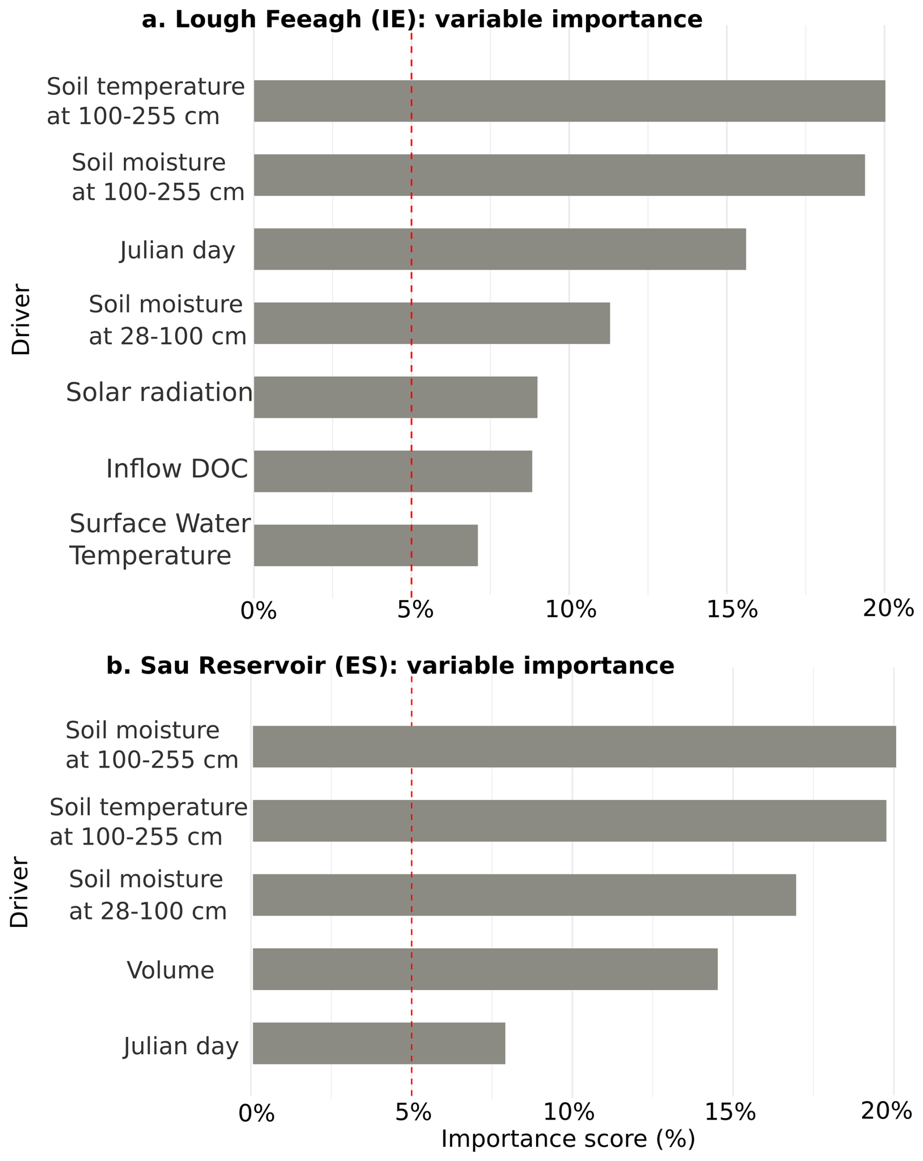
Figure 3 Selection of influential drivers for predicting fDOM. Twenty-four drivers from multiple sources were used to train the machine-learning models, including climate variables, soil variables, hydrologic and water-quality model outputs, lake model outputs, and cosine-transformed Julian day (see Fig. 2 for more details). Feature importance is shown for the best-performing model (CatBoost) using gain contribution, and drivers exceeding 5 % importance are highlighted.

3.2 Driver influence on fDOM predictions

Figure 4 introduces SHAP beeswarm plots for the most influential drivers selected in Fig. 3, enabling the assessment of the individual effect of each driver on fDOM predictions.

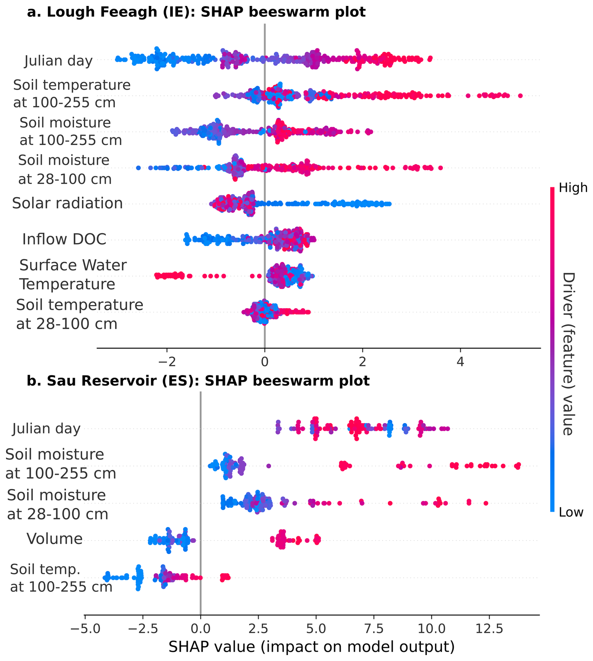
Figure 4 SHAP beeswarm plots showing the contribution of key drivers to fDOM predictions for (a) Lough Feeagh and (b) Sau Reservoir based on the CatBoost model (CTB). Points represent individual observations, coloured by feature value, and are ordered by mean absolute SHAP value.

Seasonal patterns in fDOM concentrations were observed in both Feeagh and Sau, with higher values in winter and lower in summer, as reflected in the influence of Julian day. However, the key predictors and their effects differed substantially, shaped by contrasting catchment and climate characteristics. In Feeagh, where precipitation is relatively high and sustained year-round, deep soil temperature (100–255 cm) was the dominant and potentially limiting predictor, with fDOM increasing with temperature up to a threshold, beyond which a drop in the water table may counteract the effect (see partial dependance plots; Figs. A9 and A10). In addition, Feeagh showed minimal influence of mid-depth soil temperature (28–100 cm) and solar radiation on fDOM. This temperature-fDOM relationship was less relevant in Sau, where deep soil temperature (100–255 cm) had less explanatory power. Instead, fDOM dynamics in Sau, were driven primarily by soil moisture at both 28–100 and 100–255 cm depths, potentially depicting a limiting condition by water stress.

Water availability also shaped the role of other predictors differently across the two sites. For instance, surface water temperature in Feeagh showed a clear threshold behaviour, with fDOM increasing relatively linearly beyond 6.5 °C and stabilizing around 7.5 °C, while in Sau, water volume acted as a surrogate for fDOM production (see partial dependance plots; Figs. A9 and A10). Lower volumes corresponded to reduced fDOM values, which increase and stabilize beyond 146 hm³. Interestingly, inflow DOC concentration influences Feeagh more than Sau, likely due to differences in hydroclimatological processes governing these relationships. These differences highlight how catchment water availability fundamentally alters the relative importance and behavior of fDOM drivers.

3.3 Predicting DOM using Supervised Machine Learning

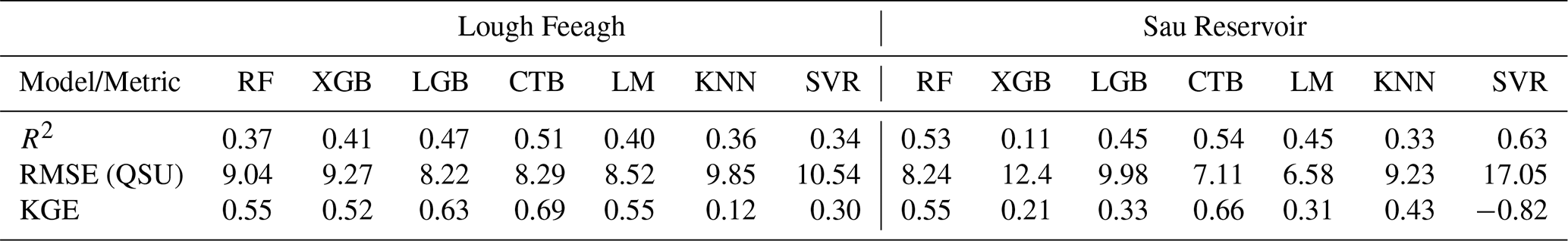
Table 1 presents a comparative evaluation of the seven ML and statistical models employed in this study. In Lough Feeagh, CatBoost (CTB) demonstrated the best overall performance with the highest R² (0.50) and KGE (0.68), and a relatively low RMSE (8.17 QSU). Similarly, in Sau Reservoir, CTB again has the highest R² (0.54) and KGE (0.66), and one of the lowest RMSE (7.11 QSU). While some models like RF and LM showed moderate performance at Feeagh, others such as SVR and XGB performed poorly in Sau, with SVR even having a negative KGE (−0.82), suggesting significant model bias. Overall, CatBoost (CTB) consistently outperformed all other models across both sites, supporting its selection for fDOM prediction using the selected environmental drivers.

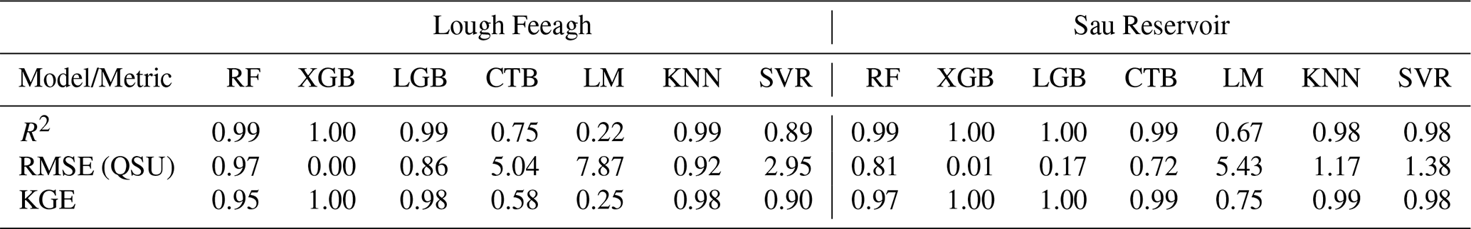
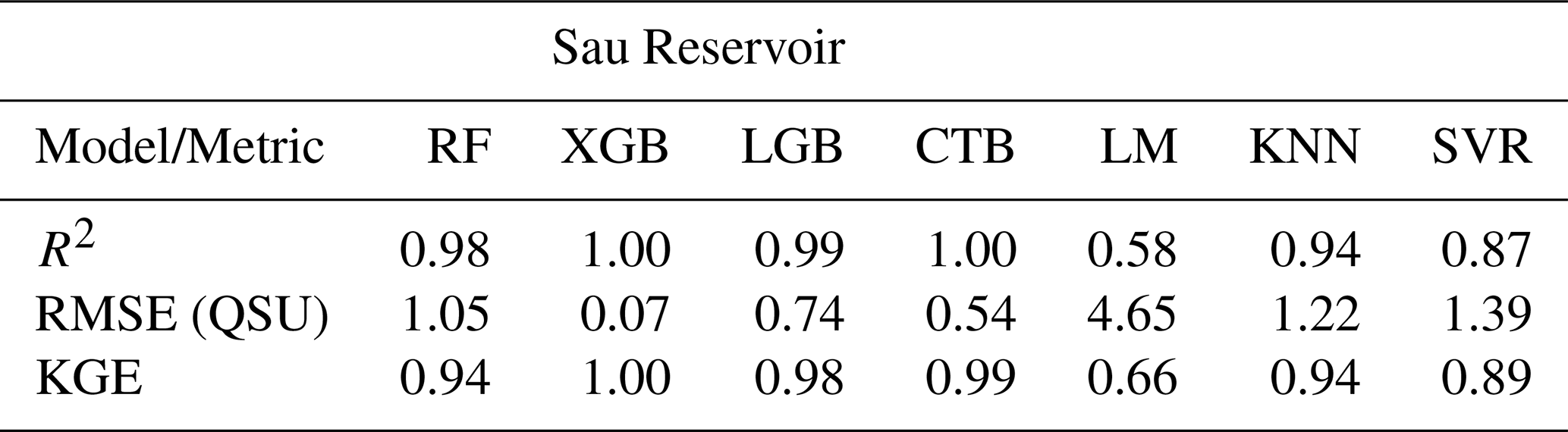
The results during the training phase (Table A2) confirm that most ML models, especially XGB, RF, and KNN, had a high performance during training. However, the performance dropped in some models (e.g., XGB at Sau Reservoir) during the testing phases, underscoring the importance of evaluating models on independent test data to assess generalisability and overfitting. CatBoost (CTB), again, presented a more stable performance, showing slightly lower training metrics (especially in Feeagh) compared with the other ML models and better generalisation when comparing with the metrics during testing. Feeagh exhibited more consistent model performance, with less overfitting between training and testing phases, across the different validation methods (Fig. A7), compared to Sau. This difference is likely attributable to the limited amount of available data at Sau. In addition, we assess whether this overfitting could be related to the moderate skewness of the fDOM data in Sau, however similar results and performance metrics were found when applying log transformation (to remove skewness) before applying the ML models (see Fig. A11 and Tables A3 and A4).

Table 1 Model comparison to predict fDOM using all selected drivers in both study sites. Statistic metrics (R², RMSE and KGE) were calculated to compare the performance of the models during the testing (hold-out) period. The table support the selection of the best model for each study site between Random Forest (RF), eXtreme Gradient Boosting (XGBoost), Light Gradient Boosting (LGB), CatBoost (CTB), k-Nearest Neighbors (KNN), Support Vector Regression (SVR) and linear model. Additionally, we tested other boosting methods, performance metrics for testing phase can be found in Table A2. Table A1 contains the results during the training period for comparison.

3.3.1 Model prediction using all drivers compared to a reduced set

Figure 5 presents the fDOM prediction performance of the CatBoost model (best ML model overall) for Feeagh and Sau, using different input configurations. The models were trained on 85 % of the time series (blue points) and tested on the remaining 15 % using a hold-out approach (violet and green points). Two scenarios were compared: one using the most influential drivers (8 for Feeagh, 5 for Sau), and a second using only a reduced subset of reanalysis-based and easily accessible drivers, specifically soil temperature, soil moisture, and Julian day.

For both lakes, the reduced driver models showed only a modest decline in predictive performance during the testing period. For example, in Feeagh, the model using all influential drivers achieved R²=0.51 and KGE = 0.69, while the reduced model still attained R²=0.48 and KGE = 0.67. Similarly, in Sau, the full model scored R²=0.54 and KGE = 0.66, whereas the reduced model maintained a comparable R²=0.50 and KGE = 0.65. Although the training performance was higher in Sau compared with the testing performance, indicating potential overfitting, the CatBoost model provided informative and generalisable predictions in both study sites.

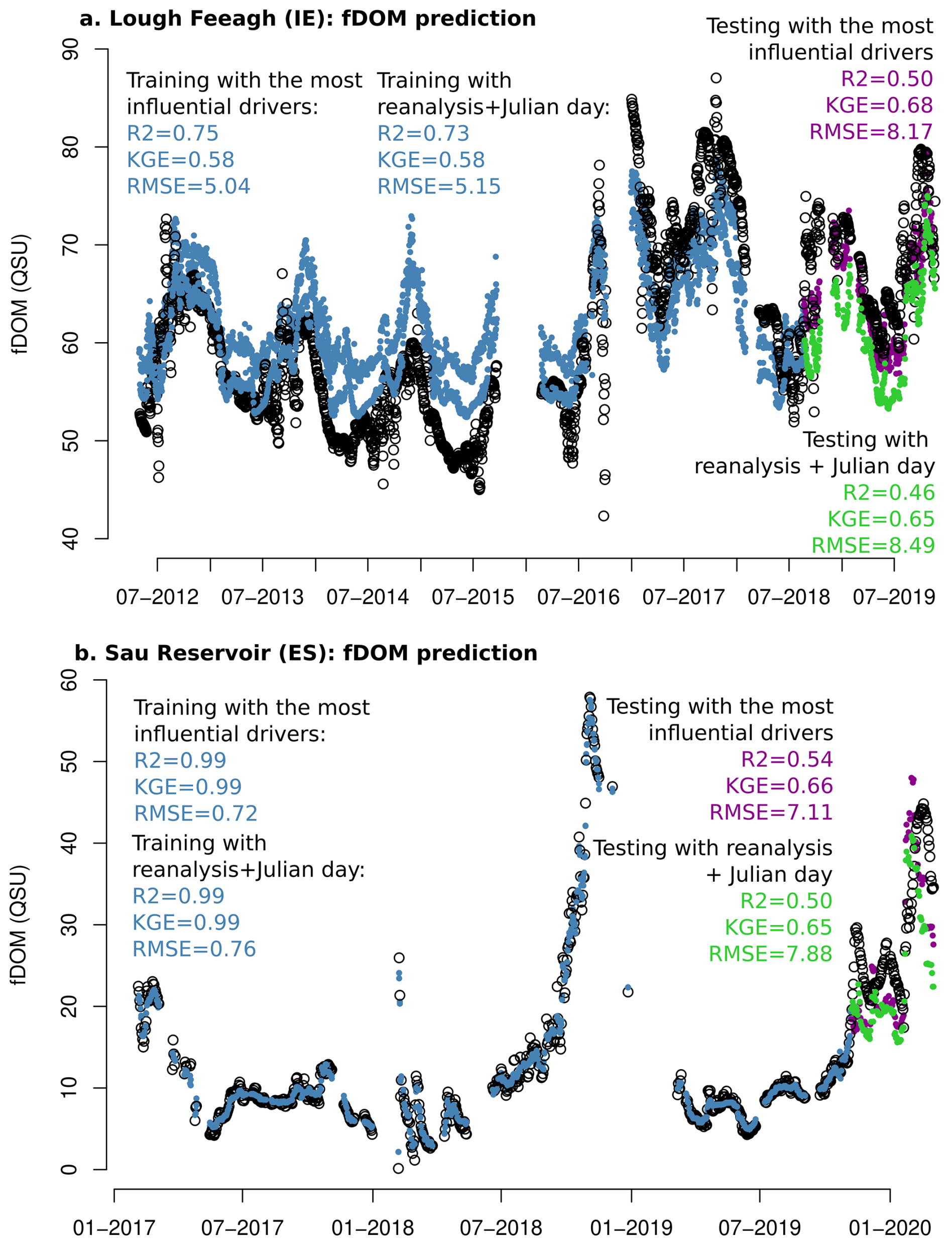
Figure 5 fDOM predictions obtained from the CatBoost model using different driver sets. Panels show training (blue; 85 % of the time series) and testing periods (violet or green; 15 %). (a) Feeagh: simulations using the most influential drivers (violet) and a reduced subset of reanalysis-based drivers + Julian day (green). (b) Sau: simulations using the most influential drivers (violet) and a reduced subset of reanalysis-based drivers + Julian day (green). Model performance metrics (R², KGE, RMSE) are reported for both periods.

4 Discussion

4.1 Driver attribution in contrasting conditions

The most influential drivers for fDOM identified for each site suggest potential carbon-producing processes that drive DOM dynamics in each lake. Interestingly, the most influential drivers were related to temperature and moisture at the deepest soil layers, indicating a common relevance for carbon inputs from terrestrial processes in both catchments. The Irish site is dominated by peat, a highly organic soil known to be sensitive to temperature-induced carbon release, especially as temperature levels rise. This is supported by the relation of soil temperatures with fDOM at this site (Ryder et al., 2014). In contrast, water availability constraints are much more pronounced in drier soils such as those of the Spanish site, as is validated by the partial dependence relationship of soil moisture with fDOM (Šimek et al., 2011). A plausible explanation is that, in Sau, increased soil moisture could boost biological activity, enhancing fDOM production, while in Feeagh, soil moisture showed a bell-shaped relationship, suggesting a more nuanced interplay between oxygen availability and microbial processes (Figs. 4, A9 and A10). In addition, higher soil moisture can reflect stronger soil–lake hydrological connectivity, particularly during wet periods and flushing events, facilitating the transport of terrestrially derived DOM into the lake.

DOM dynamics are driven by physical and biogeochemical processes in the soil that are sensitive to changes in temperature and moisture, e.g., microbial processes that break down organic matter (Kalbitz et al., 2000). The fact that the deepest layers of the soil were more important in the model for both sites than those shallower could be linked to potential carbon attenuation processes, such as soil organic matter decomposition and retention in the soil, including sorption processes (Dubeux et al., 2024; Rumpel and Kögel-Knabner, 2011). In any case, the production of carbon in the catchment that eventually ends up in the lake requires concurrent downstream transport, governed by rainfall events.

Climate and topography (see Fig. A1) dictate the flushing of accumulated DOM during rainfall events, but also can influence sustained baseflow DOM contributions. In Feeagh, carbon exports from the catchment have been observed regularly throughout the entire annual cycle, with a seasonal variability (Doyle et al., 2019). In contrast, DOM in Sau accumulates primarily during the summer and is mainly flushed out via surface runoff during the wetter winter months (Marcé et al., 2021). These patterns are supported by the relationship between inflow DOC concentration and fDOM at both sites (Figs. 4, A9 and A10), which shows a slight increase in predicted fDOM under lower carbon input conditions. Thus, inflow DOC concentration could reflect discharge pulses and dilution effects driven by precipitation (Jennings et al., 2020), following the characteristic seasonality of each site.

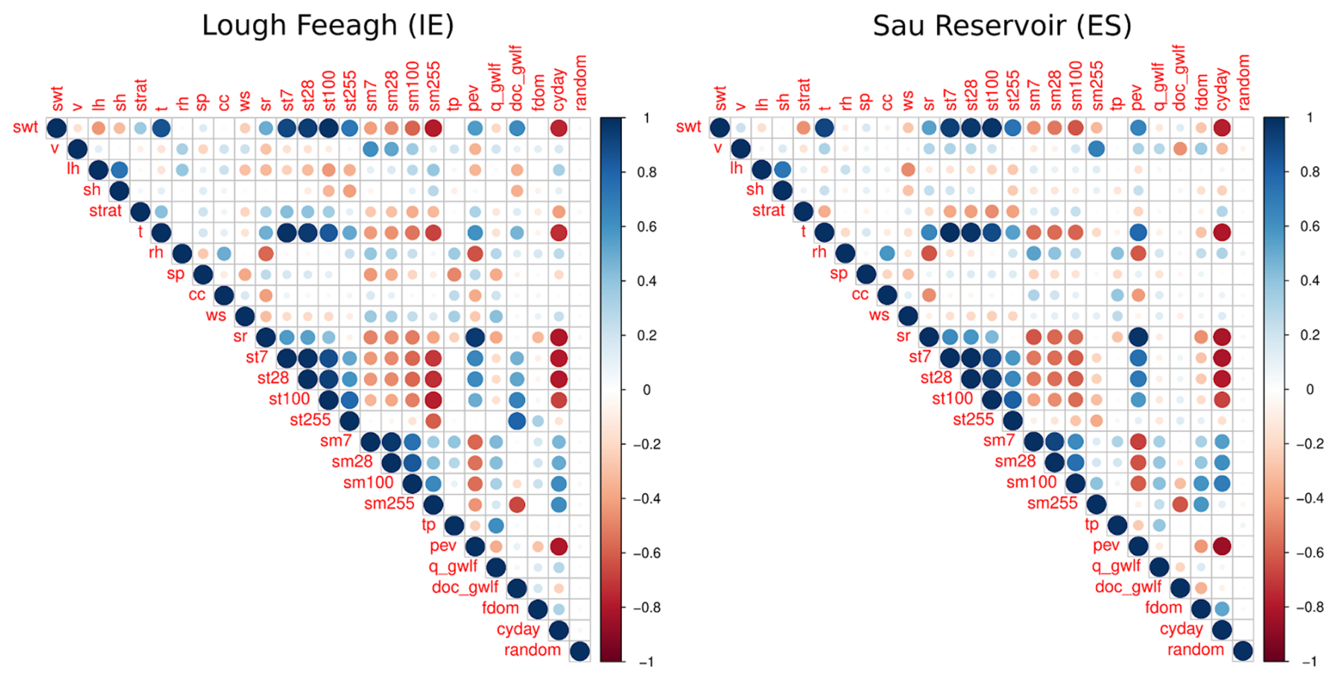
Seasonality plays a crucial role in fDOM predictions, as evidenced by the relationship of the Julian day driver with DOM dynamics at both sites (Fig. 4). At the Irish site, DOM seasonality is primarily shaped by natural environmental processes, whereas in the Spanish site, human influence plays a much greater role. This distinction helps explain why surface lake water temperature and solar radiation, two variables typically linked to strong seasonal patterns, were important only for Feeagh, while reservoir volume was significant only for Sau (Figs. 3, 4, A9 and A10). Volume and soil variables produce a similar effect on fDOM as Julian day at Sau, given that higher volumes closer to the winter season can lead to higher fDOM values. Incorporating Julian day into the workflow offers a simple yet effective way to represent seasonality, potentially replacing seasonal variables (e.g., air temperature) (see the correlation matrix of all drivers in Fig. A12). This proves that the use of machine learning approaches opens up opportunities to assess diverse drivers under contrasting conditions.

Improving the accuracy of DOM predictions in lakes can enhance efforts to reduce further water quality deterioration and support lake management. This study demonstrated a feasible approach for simulating daily fDOM in two contrasting lakes, especially when using the Catboost model given its good generalisability. The performance metrics (Fig. 5) obtained at each site for the different model simulations lie in a similar or better range than comparable studies that modelled carbon dynamics in lakes (e.g., Harkort and Duan, 2023; Liu et al., 2021; Zhang et al., 2021, 2024). It is important to be aware, however, that previous studies are based on different frameworks. These include variations in the machine learning algorithms used, the target variable for quantifying carbon dynamics, with most studies having focused on DOC, whereas fDOM is the target variable here, as well as differences in input driver data and site-specific conditions. While both fDOM and DOC are widely used indicators of dissolved organic matter in lakes, they differ in measurement principles and in the fractions of organic matter they represent. Both variables, however, remain ecologically relevant for understanding DOM sources, transport, and transformation processes, which aligns with the context of this work.

4.2 Scalability

Our results suggest high potential for scalability, as predictive performance remained consistent across different driver sets even for two contrasting study sites, and performed good using only reanalysis data that is globally available and Julian day (Fig. 5). Importantly, this consistency remained even when specific highly-influential drivers were removed from the driver set. For instance, in Sau, where human intervention makes future reservoir outflows difficult to predict, avoiding reliance on water volume as a driver proved advantageous, as its removal from the set of drivers maintained model performance, despite being identified as an influential variable. It is likely that soil moisture at the deepest layer, a variable that showed a behavior similar to that of volume (Fig. 4), may have contributed to maintain the predictive performance when volume is removed from the driver set. In addition, for Feeagh, the predictive capacity was also maintained when using only meteorological and soil drivers. This demonstrates that a large driver dataset, such as the 24-variable set used in this study, would not be necessary to produce an accurate prediction when modelling fDOM using supervised machine learning.

4.3 Limitations and future research

Our approach offers the opportunity to validate and deploy a workflow capable of delivering daily DOM predictions in both undisturbed and anthropized sites, even when only limited data on input drivers are available, while at the same time providing insights into the dominant drivers. However, a site-specific model validation, including identification of appropriate training and testing periods, hyperparameter tuning for each specific study site and assessment of overfitting is essential. In terms of driver attribution, it is of note that the relationships identified using machine learning may not always be related at a process level (Sullivan, 2022). In our case, however, many of these same drivers had already been identified for river DOC levels in the Feeagh catchment (e.g., Doyle et al., 2019; Ryder et al., 2014). While the workflow can be easily replicated, fDOM data or data for another proxy for DOM are required. It is of note that such proxies of DOM are increasingly being incorporated into water quality monitoring programmes, an aspect that is convenient for testing workflows such as the one described (Downing et al., 2012).

The workflow presented here is not recommended for climate change studies, as the drivers of DOM variability can significantly change under entirely new and unrecorded climatic conditions. Consequently, supervised machine learning may fail to capture the signal from the time series. Moreover, the method's reliance on historical patterns limits its ability to extrapolate beyond the range of observed environmental conditions (Mi et al., 2024). Future research could expand the application of this framework to a broader range of lakes, integrate additional drivers such as remote sensing-derived terrestrial and aquatic quantity and quality parameters (Duan et al., 2025).

5 Conclusions

By identifying the key environmental drivers of lake dissolved organic matter (DOM) dynamics, this study presents an open, robust and scalable workflow for daily DOM prediction using different ML algorithms. Validated in two hydroclimatic contrasting sites in Ireland (Lough Feeagh) and Spain (Sau Reservoir), the approach revealed that deep soil temperature is the dominant driver in the peat-rich, temperate Irish catchment, whereas deep soil moisture plays a more critical role in the drier, Mediterranean setting of the Spanish site. These primary drivers are further shaped by hydrological processes, seasonal variability, and human activities.

The workflow showed good predictive performance even when based solely on globally available reanalysis data, supporting its potential applicability to other freshwater systems worldwide. In addition to expanding the set of approaches available for lake DOM prediction, the workflow offers transparent driver attribution, contributing valuable insights into the natural and anthropogenic processes governing carbon cycling in aquatic ecosystems.

Appendix A

A1 Topography of Feeagh and Sau catchments

Figure A1 contains the elevation range for the two contrasting freshwater ecosystems: Lough Feeagh and Sau Reservoir.

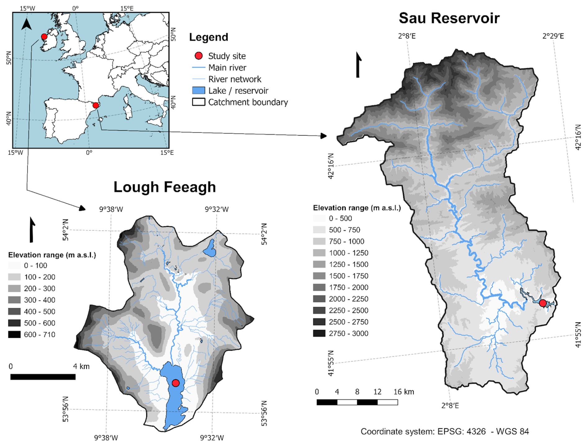
Figure A1 Elevation range for the two contrasting freshwater ecosystems: Lough Feeagh and Sau Reservoir.

A2 CORINE land-cover classes and aggregation for both study catchments

Here, we present Fig. A2 listing all original CORINE Land Cover 2018 classes identified within each catchment and their aggregation into the grouped categories used in Fig. 1. These tables show how individual CORINE classes were consolidated to represent dominant catchment characteristics while maintaining consistency with the original CORINE classification. This information supports the visual interpretation presented in Fig. 1.

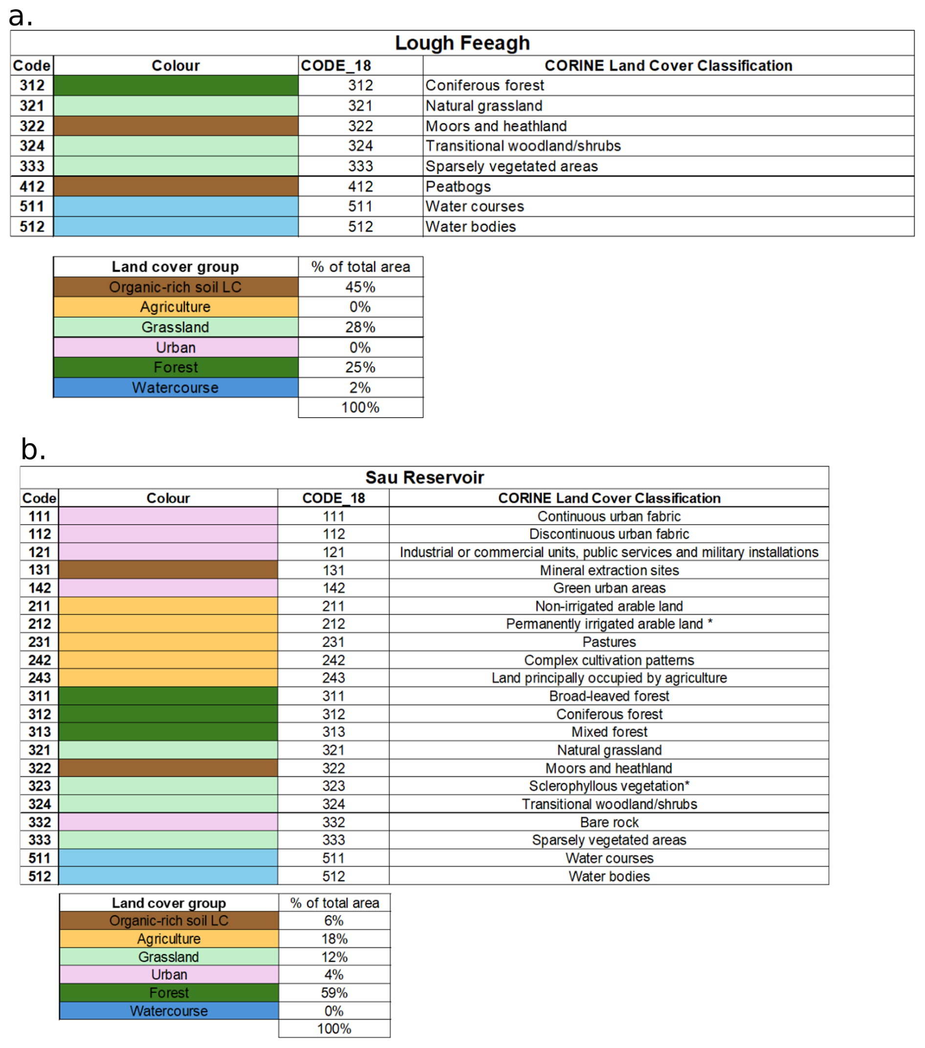
Figure A2 (a) CORINE Land Cover 2018 classes identified in Feeagh and the grouped categories shown for visual clarity in the main manuscript in Fig. 1; (b) CORINE Land Cover 2018 classes identified in Sau and the grouped categories shown for visual clarity in the main manuscript in Fig. 1.

A3 Data inspection and exploration

Data inspection and exploration: the target variable (fDOM) at one of the study sites (Feeagh) exhibits low to moderate skewness (approximately 0.5) with relatively few outliers, whereas the other study site (Sau) displays higher skewness (greater than 1 but below 2) and several extreme values. Zero-inflation does not appear to be an issue at either site.

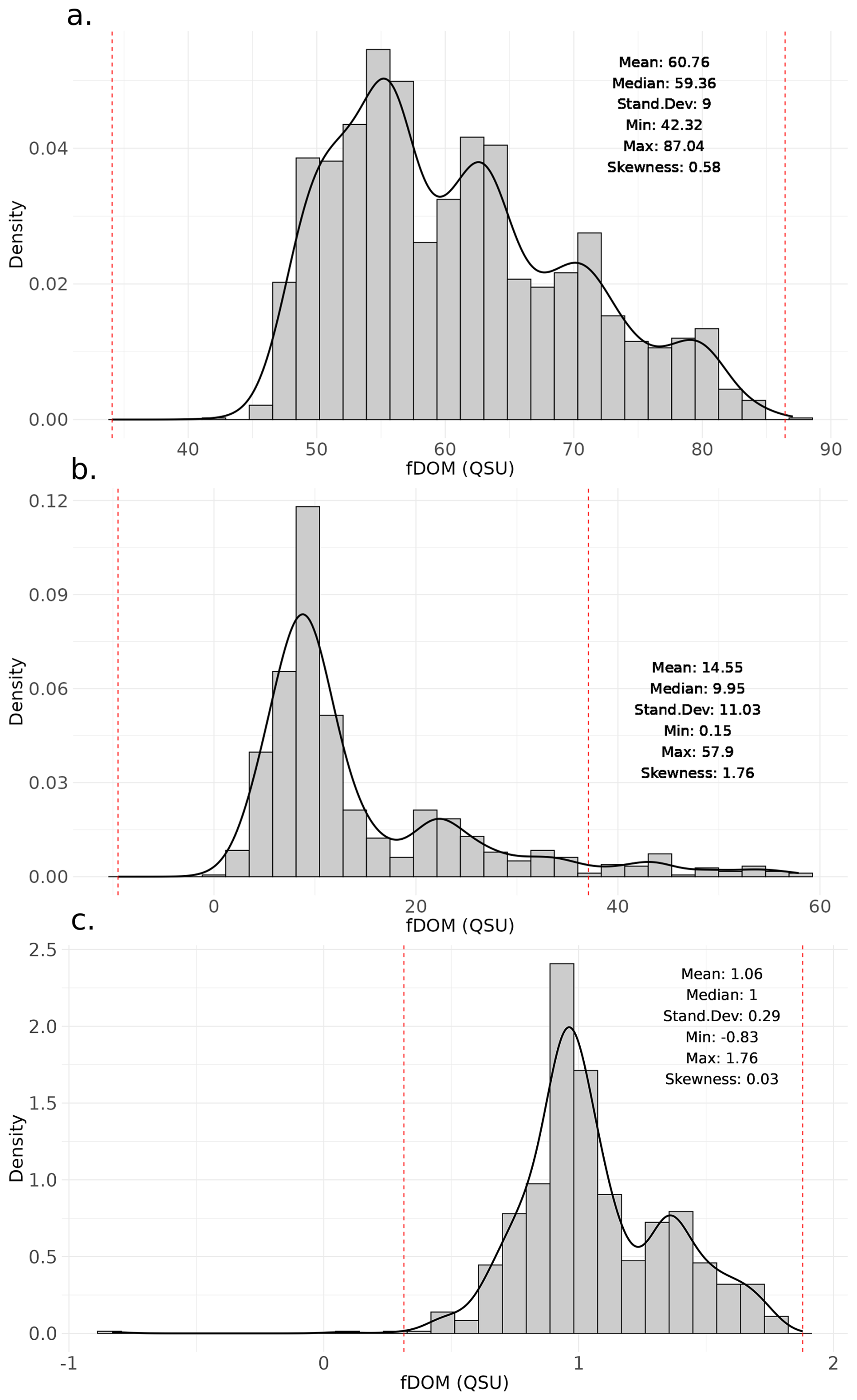
Figure A3 Exploratory data analysis for fDOM in both study sites, (a) Shows the density plot of fDOM in Feeagh and (b) Shows the density plot of fDOM in Sau, (c) Shows the density plot of fDOM in Sau using log₁₀ transformation. The red vertical line separates the outliers.

A4 Water temperature correction of fDOM for both study sites

In Feeagh, fDOM data was corrected for the temperature quenching effect in previous scientific studies. The raw measurements were corrected using the compensation approach described by (Watras et al., 2011; Ryder et al., 2012). Corrected fluorescence was calculated relative to a reference temperature of 20 °C using: $\text{Corrected fDOM}=\frac{\text{raw fDOM}}{\mathrm{1}+(T-\mathrm{20})k}$ where T is the sonde water temperature (°C) and k is the temperature correction coefficient (k=−0.0168 for Feeagh, derived as the average of monthly values reported by Ryder et al. (2012)).

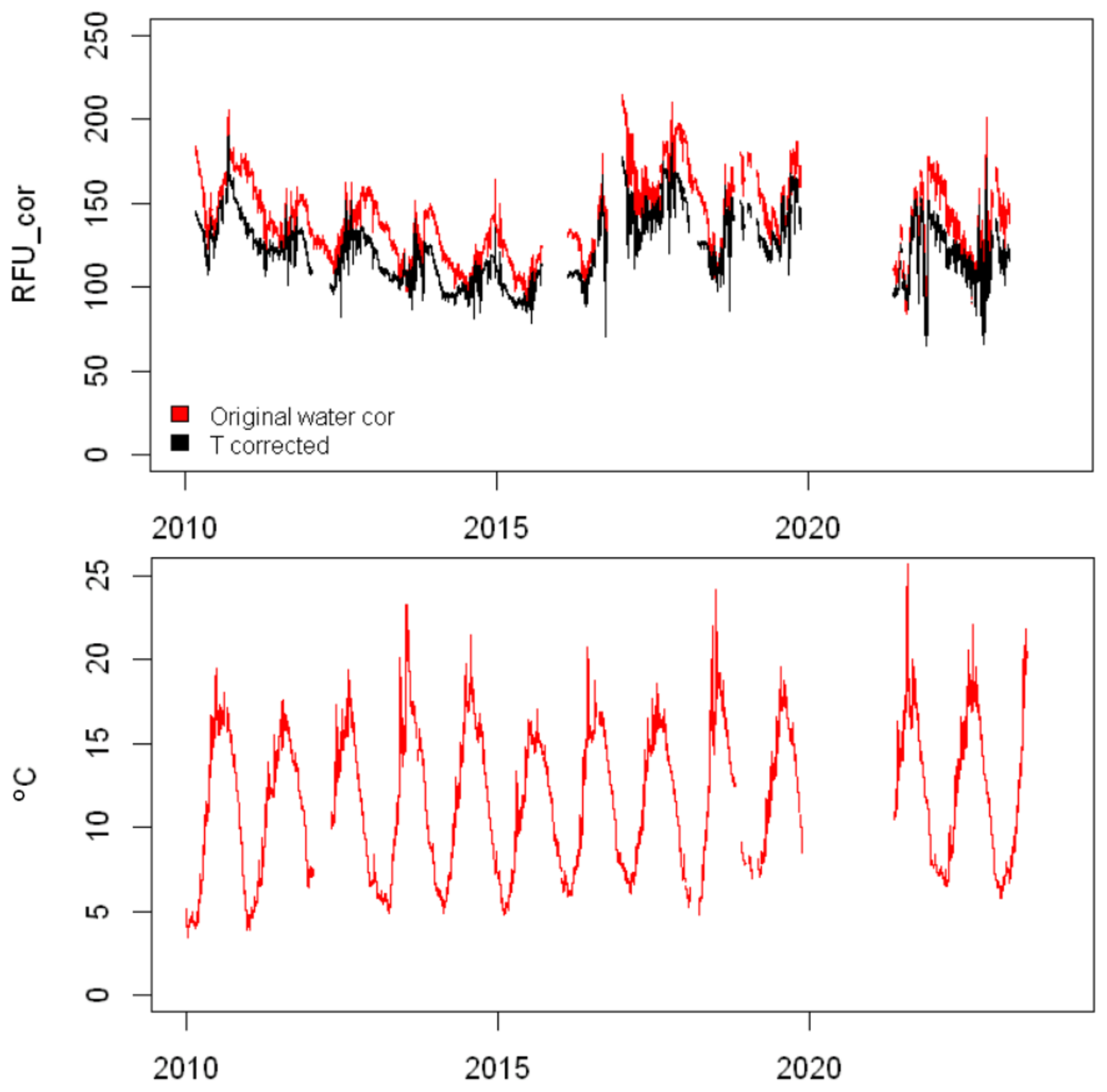
Figure A4 Upper panel: Raw (blue) and temperature-corrected (red) fDOM measurements for Feeagh; lower panel: surface water temperature sonde measurements at Feeagh.

In Sau, the fDOM data were corrected for the temperature quenching effect, following a test provided by the fDOM sensor manufacturer, where they use a 300 QSU sample of water and change the temperature to get the effect of temperature in the measurement, results can be found in Fig. A5.

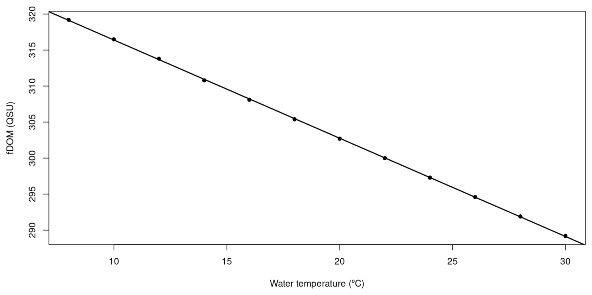
Figure A5 fDOM relation with temperature with a sample of 300 QSU provided by the manufacturer of the fDOM sensor in Sau.

Figure A6 Uncorrected (blue) and corrected (red) fDOM data for Sau.

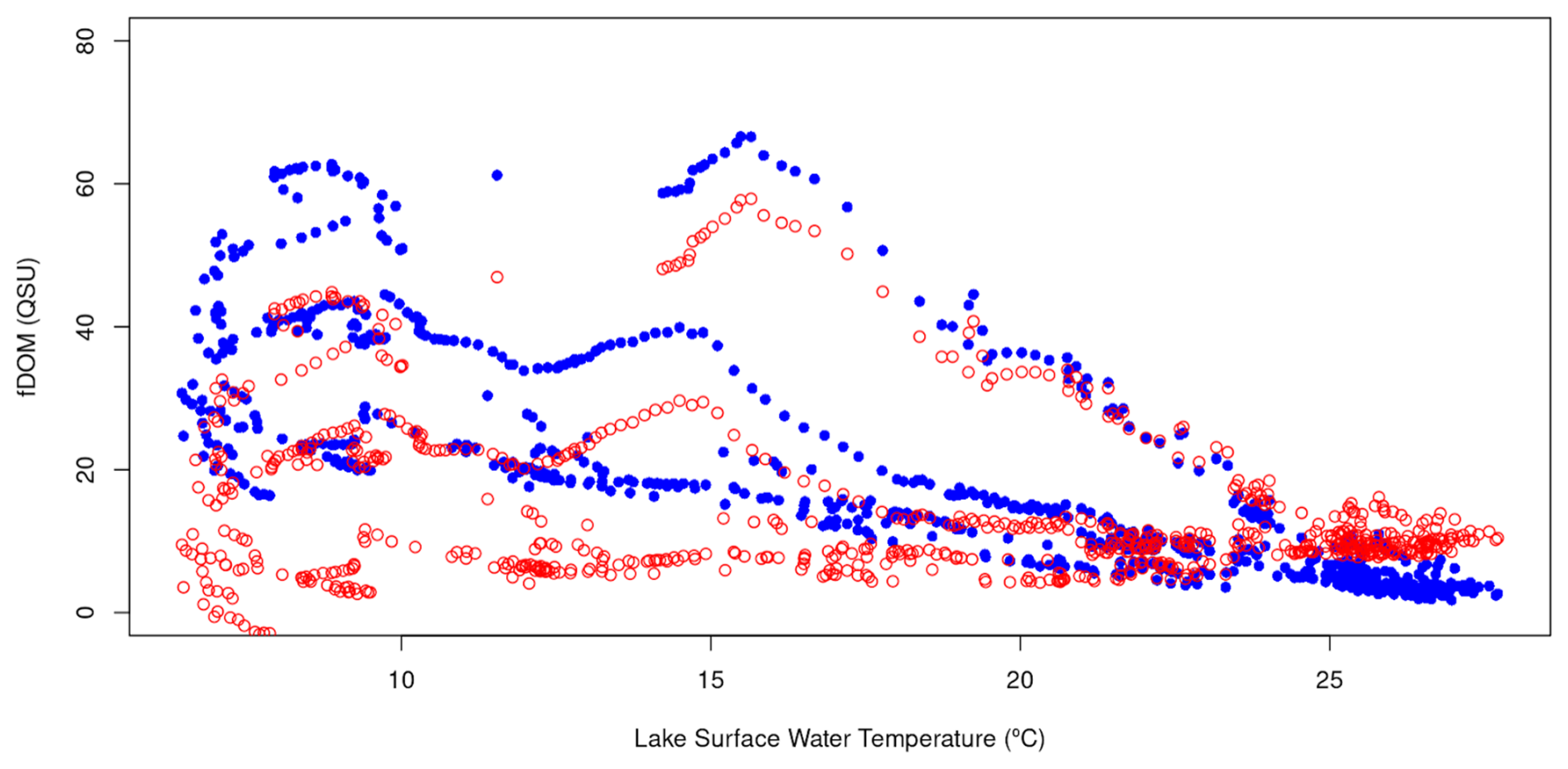
Then, fDOM data in Sau was corrected following this linear regression and surface water temperature on the lake. Figure A6 presents the uncorrected values in blue and corrected values in red (8 negative values were removed from the total sample of 777)

A5 Hydrologic Modelling

Daily time series of inflow discharge and inflow DOC concentration into each site were generated using the Generalised Watershed Loading Functions Model (GWLF) coupled with a DOC module (GWLF-DOC). This model simulates catchment hydrology (water balance and water distribution among the different hydrological pathways) and DOC dynamics (DOC production and DOC washout) in a daily time step. The model input requirements include daily time series of two meteorological variables: total precipitation and air temperature; as well as land cover, land use, and soil characterisation.

GWLF-DOC was applied to Feeagh based on previous model applications in the Irish catchment (Paíz et al., 2025a), for which measured discharge data were used to calibrate and validate the hydrology (2013–2018 and 2019–2023, respectively), and DOC concentration data were used to calibrate the DOC module (2016–2023). In Sau, observed inflow discharge data were used to calibrate and validate the hydrology (2008–2011 and 2011–2024, respectively), and measured DOC concentration data were used to calibrate and validate the DOC module (2008–2014 and 2016–2018, respectively) using the same calibration strategy than for the Irish site. Calibration results were satisfactory for both hydrology (Feeagh: R²=0.64 and NSE = 0.64; Sau: R²=0.66 and NSE = 0.66;) and DOC (Feeagh: R²=0.45 and NSE = 0.47; Sau: R²=0.44 and NSE = 0.40). Similarly, validation results were satisfactory for both hydrology (Feeagh: R²=0.60 and NSE = 0.60; Sau: R²=0.42 and NSE = 0.42) and DOC in the case of Sau (R²=0.50 and NSE = 0.46).

A6 Lake Modelling

Daily time series of 5 key lake variables (see Fig. 2) were obtained from the General Lake Model (GLM) run for each site. GLM is an open-source, one-dimensional hydrodynamic model designed to simulate the vertical stratification and water balance of lakes and reservoirs. It calculates vertical profiles of temperature, and density by accounting for factors such as inflows and outflows, mixing processes, and surface heating and cooling (Hipsey et al., 2019). GLM was calibrated and validated by evaluating the fit of modelled water temperature against measured water temperature profile data in Feeagh (2010–2015 and 2016–2017, respectively) and Sau (1997–2007 and 2008–2018, respectively). The calibration strategy was based on previous lake modelling deployments at each site (Mercado-Bettín et al., 2021; Paíz et al., 2025b). Model performance was satisfactory for both sites.

A7 Comparison of validation methods using Random Forest

To pick the most suitable validation method, we implemented hold-out period method used in the main manuscript, k-fold cross-validation method using k=5, and rolling window cross-validation using training size of two year, testing size of one year, and a shift window every 90 d. Results are shown in Fig. A7.

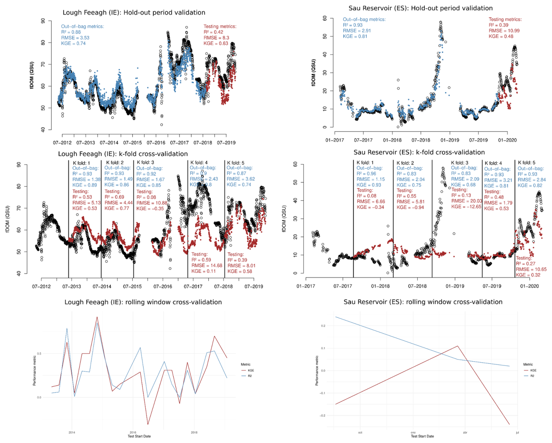
Figure A7 Comparison of validation methods using random forest for both study sites: hold-out period method used in the main manuscript, k-fold cross-validation method using k=5, and rolling window cross-validation using training size of two year, testing size of one year, and a shift window every 90 d. For this method, in the case of Sau Reservoir it is not possible to get a clear analysis due to the limited data.

A8 Identification of most influential drivers

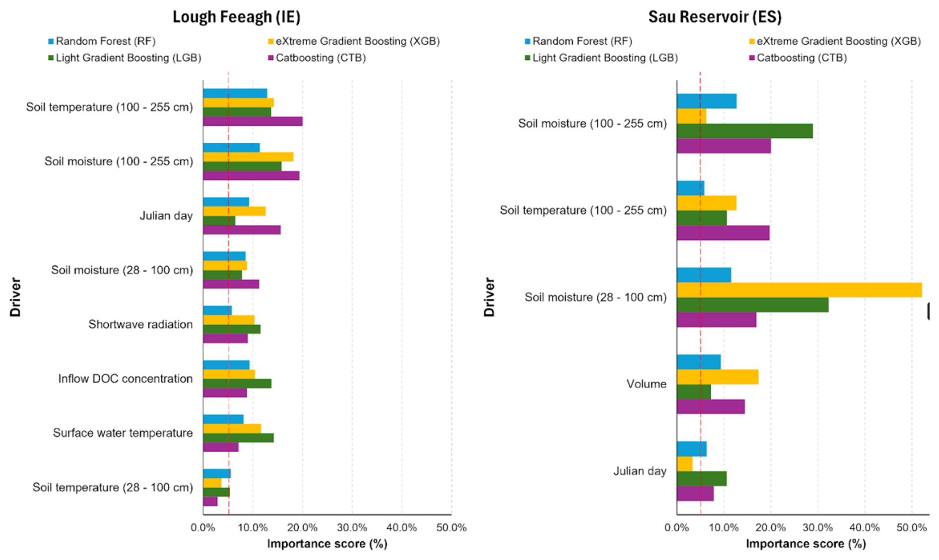
Figure A8 Selection of influential drivers for predicting fDOM. Twenty-four drivers from multiple sources were used to train the machine-learning models, including climate variables, soil variables, hydrologic and water-quality model outputs, lake model outputs, and cosine-transformed Julian day. Feature importance is shown for four models Random Forest, Light Gradient Boosting, eXtreme Gradient Boosting and Catboosting, and drivers exceeding 5 % importance are highlighted.

A9 Partial dependence plots for the most influential drivers

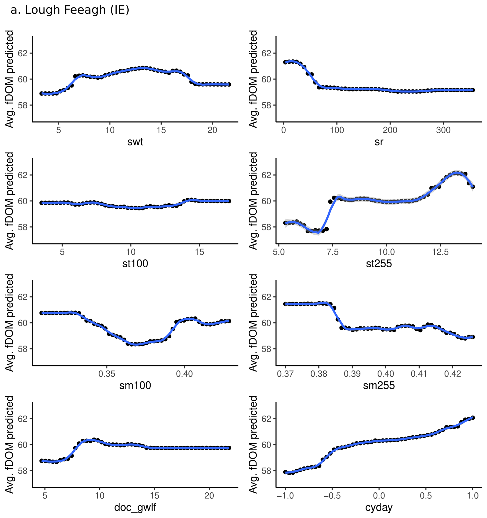
Figure A9 Partial dependence plots for the most influential drivers (feature importance > 5 %, estimated using node purity) based on Random Forest model outputs for Lough Feeagh. Cosine-transformed Julian day (cyday) values are shown for seasonality; approximate calendar timing corresponds to cos(Julian day) ≈ 1 (winter), 0 (spring/autumn), and −1 (summer).

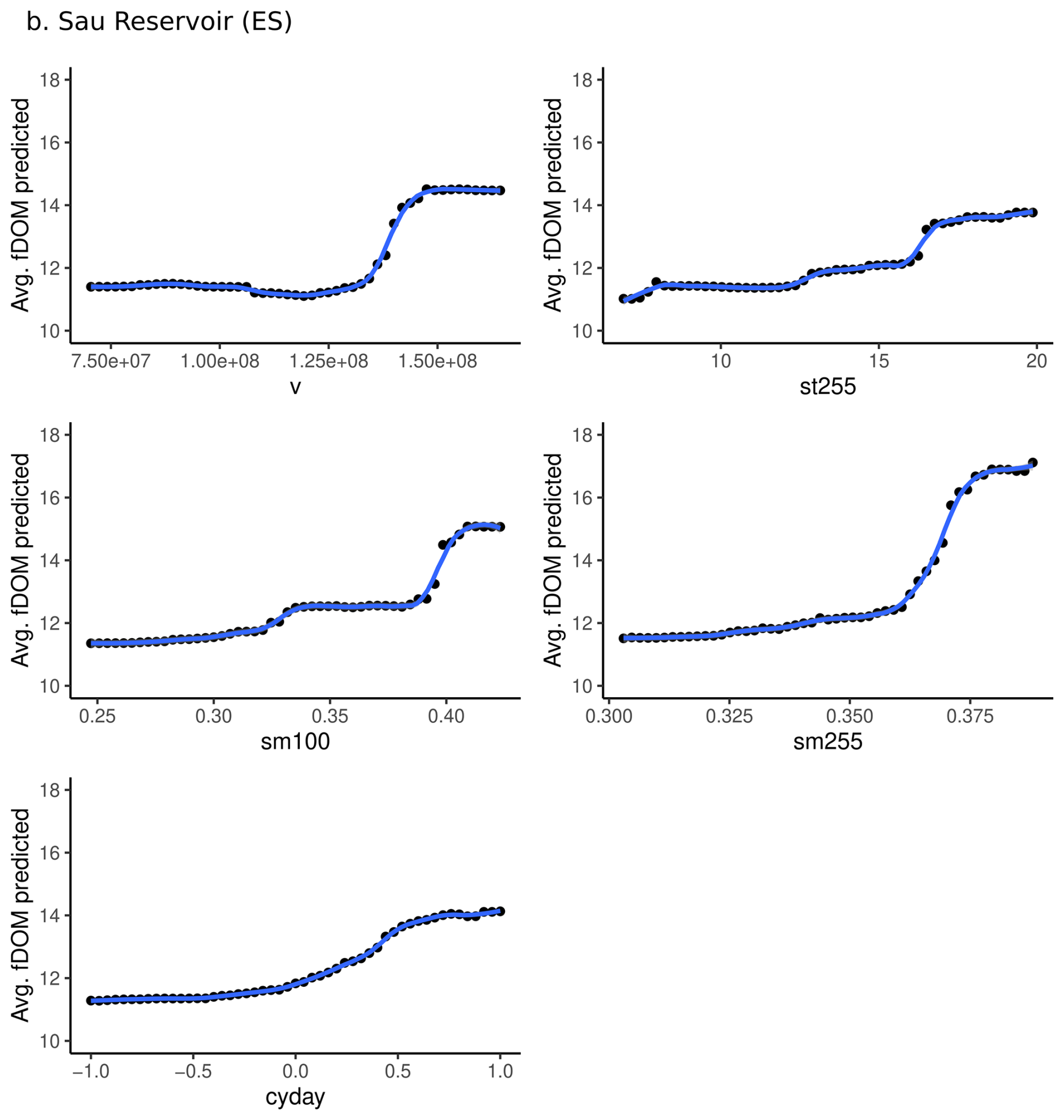
Figure A10 Partial dependence plots for the most influential drivers (feature importance > 5 %, estimated using node purity) based on Random Forest model outputs for Sau Reservoir. Cosine-transformed Julian day (cyday) values are shown for seasonality; approximate calendar timing corresponds to cos(Julian day) ≈ 1 (winter), 0 (spring/autumn), and −1 (summer).

A10 Result for Sau Reservoir using log₁₀ transformation

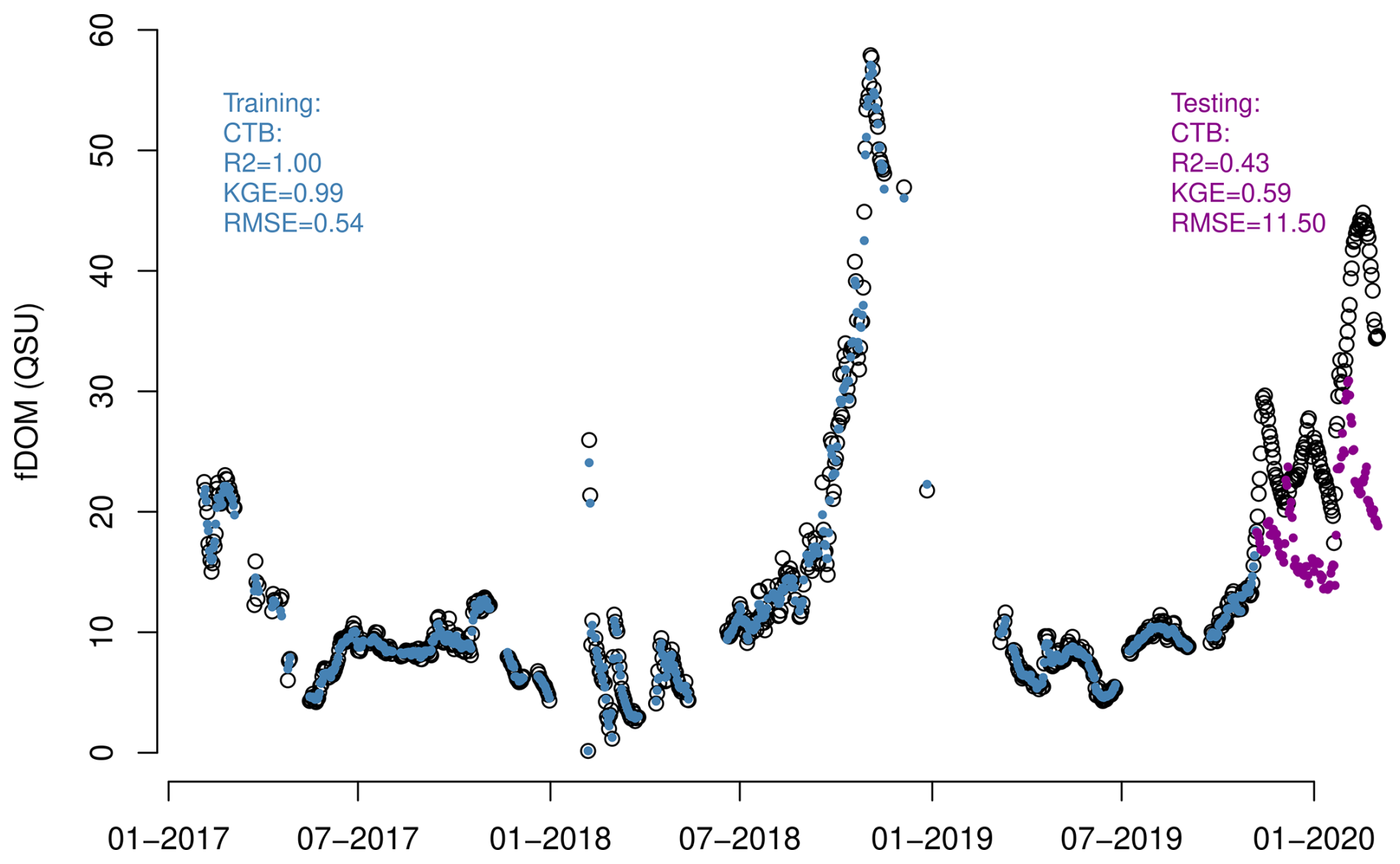
Figure A11 fDOM predictions obtained from the boosting (CatBoost) model using the most influential drivers with initial log₁₀ transformation of the fDOM data.

A11 Correlation matrix of all drivers and fDOM for Feeagh and Sau.

Correlation matrix of all drivers is presented in Fig. A12.

Figure A12 Correlation matrix of all drivers and fDOM for Feeagh and Sau.

A12 Model comparison to predict fDOM using the most influential drivers in both study sites.

Resulting metrics during testing and training periods for all models are shown in Tables A1 and A2, respectively.

Table A1 Model comparison during testing to predict fDOM using all selected drivers in both study sites. Statistic metrics (R², RMSE and KGE) were calculated to compare the performance of the models Random Forest (RF), eXtreme Gradient Boosting (XGBoost), Light Gradient Boosting (LGB), Catboosting (CTB), k-Nearest Neighbors (KNN), Support Vector Regression (SVR) and linear model during training period.

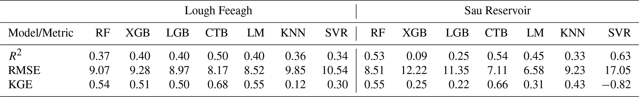
Table A2 Model comparison during training to predict fDOM using all selected drivers in both study sites. Statistic metrics (R², RMSE and KGE) were calculated to compare the performance of the models Random Forest (RF), eXtreme Gradient Boosting (XGBoost), Light Gradient Boosting (LGB), Catboosting (CTB), k-Nearest Neighbors (KNN), Support Vector Regression (SVR) and linear model during training period.

A13 Model comparison to predict fDOM using the most influential drivers in Sau with previous application of log₁₀ transformation

Tables A3 and A4 presents the testing and training performance metrics results for Sau site with previous application of log₁₀ transformation.

Table A3 Model comparison during testing to predict fDOM using the most influential drivers in Sau with previous application of log₁₀ transformation. Statistic metrics (R², RMSE and KGE) were calculated to compare the performance of the models Random Forest (RF), eXtreme Gradient Boosting (XGBoost), Light Gradient Boosting (LGB), Catboosting (CTB), k-Nearest Neighbors (KNN), Support Vector Regression (SVR) and linear model during training period.

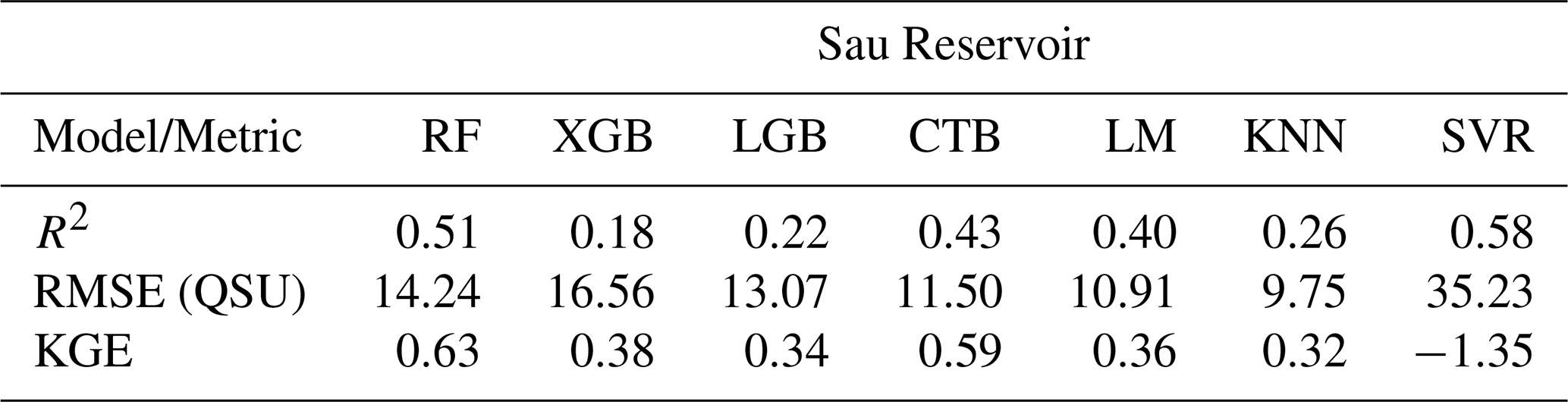
Table A4 Model comparison during training to predict fDOM using the most influential drivers in Sau with previous application of log₁₀ transformation. Statistic metrics (R², RMSE and KGE) were calculated to compare the performance of the models Random Forest (RF), eXtreme Gradient Boosting (XGBoost), Light Gradient Boosting (LGB), Catboosting (CTB), k-Nearest Neighbors (KNN), Support Vector Regression (SVR) and linear model during training period.