Dynamics of island mass effect – Part 2: Phytoplankton physiological responses

Island mass effect (IME) refers to the phenomenon of elevated chlorophyll a concentrations around islands, often extending hundreds of kilometers into oligotrophic waters. In this study, we explore the physiological responses and changes in phytoplankton community composition within island mass effect zones, providing insights into the drivers and ecological impacts of this phenomenon. Here, we study IMEs associated with four South Pacific subtropical archipelagos over six-month periods. We use a combination of satellite-derived physiological indices and in situ bio-optical data collected during the Tara Pacific expedition (2016–2018) to further our mechanistic understanding of IME. We examine mechanisms such as nutrient enrichment and pigment-based proxies of ecological succession that underpin the IME. Our results demonstrate that phytoplankton populations within IME zones typically experience reduced physiological stress compared to the surrounding open ocean, likely due to an alleviation of iron limitation. Hence, recurring iron enrichment may be a significant factor of IME across the South Pacific Subtropical Ocean. In some cases, we also detected signatures of decreased phytoplankton stress due to macronutrient limitation associated with local upwellings and increased vertical mixing, highlighting the role of physical processes in supplying macronutrients to the photic zone. While iron enrichment seems to originate mostly from terrigenous/reef inputs, macronutrients can be both from terrigenous/reef origin or vertical entrainment of nutrient-rich deep water to the surface ocean. We also show that IME is often associated with changes in pigment ratios, which is suggestive of changes in phytoplankton community composition. These findings underscore the complex interplay between nutrient availability, community composition, and physiological stress in shaping IME, offering new perspectives on this phenomenon and its ecological significance.

1 Introduction

The island mass effect (IME) refers to different processes that result in the enhancement of chlorophyll a concentration [Chl a] and phytoplankton biomass around islands, relative to their surrounding ocean. This phenomenon can contribute substantially to regional phytoplankton standing stocks and may have significant impacts on biogeochemical processes and food web dynamics in oligotrophic oceans (Gove et al., 2016; Messié et al., 2022; Bourdin et al., 2025). De Falco et al. (2022) suggest that sea surface temperature (SST) anomalies around large elevated islands are due to upwelling and downwelling processes, while smaller islands exhibit only localized cooling from current-island interactions. These patterns indicate that multiple nutrient-enriching processes can coexist around a single island, varying seasonally with oceanic and atmospheric forcing. Single-archipelago studies have shown that macronutrient and iron enrichment in the euphotic zone in the vicinity of islands can lead to phytoplankton biomass accumulation and IME formation (Messié et al., 2020; Martinez et al., 2020; Caputi et al., 2019; James et al., 2020; Palacios, 2002; Raapoto et al., 2019; Signorini et al., 1999). Additionally, Martinez et al. (2020) found differences in plankton community composition between island-specific IME events within the Marquesas archipelago, and indicated that interactions between bottom-up nutrient enrichments and top-down control of phytoplankton populations by grazers can be important factors driving IME processes.

To date, most basin-scale studies of IME have relied on [Chl a] (Gove et al., 2016; Messié et al., 2022; Bourdin et al., 2025) or chlorophyll fluorescence (Dandonneau and Charpy, 1985) to assess phytoplankton biomass, offering valuable insights into the spatial extent and temporal variability of IME, but without explicitly disentangling the underlying contributing factors. Because variations in [Chl a] can result from changes in phytoplankton biomass, community composition (Langdon, 1988), and physiological acclimation to nutrients, SST, and light (Geider et al., 1998; Geider, 1987), the interpretation of [Chl a] as a phytoplankton biomass indicator is susceptible to bias if not concurrently evaluated with other independent proxies of phytoplankton biomass. Such metrics could include proxies for particulate organic carbon (POC; Bishop et al., 1999; Gardner et al., 2003, 2006) or phytoplankton carbon (C_phyto; Graff et al., 2015; Behrenfeld and Boss, 2006), which are insensitive to photoacclimation and can be retrieved from satellite observations. Furthermore, because phytoplankton intracellular [Chl a] synthesis is upregulated when incident light decreases and downregulated when phytoplankton cells are stressed due to nutrient limitation, we can use the ratio of [Chl a] to C_phyto ($\frac{\left[\mathrm{Chl}a\right]}{C_{\mathrm{phyto}}}$) to estimate physiological responses to light exposure and nutrient enrichment (Behrenfeld et al., 2015; Halsey and Jones, 2015; Laws and Bannister, 1980). With information about ambient light and the mixing depth, we can estimate the contribution of photoacclimation to $\frac{C_{\mathrm{phyto}}}{\left[\mathrm{Chl}a\right]}$ and therefore deduce information about physiological responses to nutrient availability. Moreover, multiple studies have shown that iron limitation has a distinct signature on phytoplankton fluorescence, with cells under iron limitation exhibiting higher chlorophyll fluorescence for a given incident irradiance and light absorption efficiency (Behrenfeld and Kolber, 1999; Behrenfeld et al., 2006; Greene et al., 1994; Kolber et al., 1994; Olson et al., 2000; Behrenfeld and Milligan, 2013). Behrenfeld et al. (2009) used this characteristic to calculate the fluorescence quantum yield (Φ_Sat) from remote sensing data and assess phytoplankton iron stress across ocean basins.

Building on these relationships, new insights into phytoplankton physiology can be gained in the context of the IME. Here, we examine spatial and temporal variations in macronutrient and iron stress responses of phytoplankton, comparing between communities in coastal water of islands, communities in water masses under the influence of the IME that have been advected offshore, and communities in the adjacent background oligotrophic ocean. We integrate high-resolution in situ bio-optical proxies with satellite data to assess the covariance between nutrient stress responses, biomass increases, and potential shifts in phytoplankton community composition. This integrated analysis allows us to generate hypotheses related to the type and origin of nutrient enrichments associated with the IME and to evaluate their ecological consequences for surface plankton communities.

To capture the spectrum of IME responses across the South Pacific Subtropical Gyre (SPSG), this paper presents observations from four archipelagos (Rapa Nui, Society Islands, Samoa, and Fiji) with varying size, bathymetry, elevation, geographical position, and which are associated with a wide range of IME spatial and temporal extents and [Chl a] enhancement (Bourdin et al., 2025). This approach allows a more mechanistic understanding of the likely processes driving the IME. While this method is presented here in the context of the IME, it is applicable to other studies of mesoscale processes in the ocean, such as upwelling systems and river discharge.

2 Method

2.1 Case study islands

We selected four study regions distributed along a longitudinal gradient of the subtropical and tropical South Pacific Ocean. These regions were sampled as part of the basin-scale survey conducted during the Tara Pacific expedition (2016–2018; Gorsky et al., 2019; Lombard et al., 2023). The selected regions span a gradient of oceanographic conditions, ranging from the ultra-oligotrophic eastern basin (near Rapa Nui) to the moderately oligotrophic Western Pacific Basin (near Fiji and Tonga). Island densities, size, and geomorphic types vary between and within these regions (Fig. 1). For instance, the region studied around Rapa Nui in the Eastern Pacific encompasses 2 islands and 3 submerged reefs, while the region studied around Fiji and Tonga in the Western Pacific encompasses 158 islands and 306 submerged reefs.

The spatial and temporal dynamics of IMEs and their associated chlorophyll a enhancement have been characterized for each of these case study regions (Bourdin et al., 2025). Here, we extend this analysis to include physiological indicators derived from bio-optical and remote sensing measurements to gain new insights about the underlying mechanisms that contribute to the observed chlorophyll a enhancement.

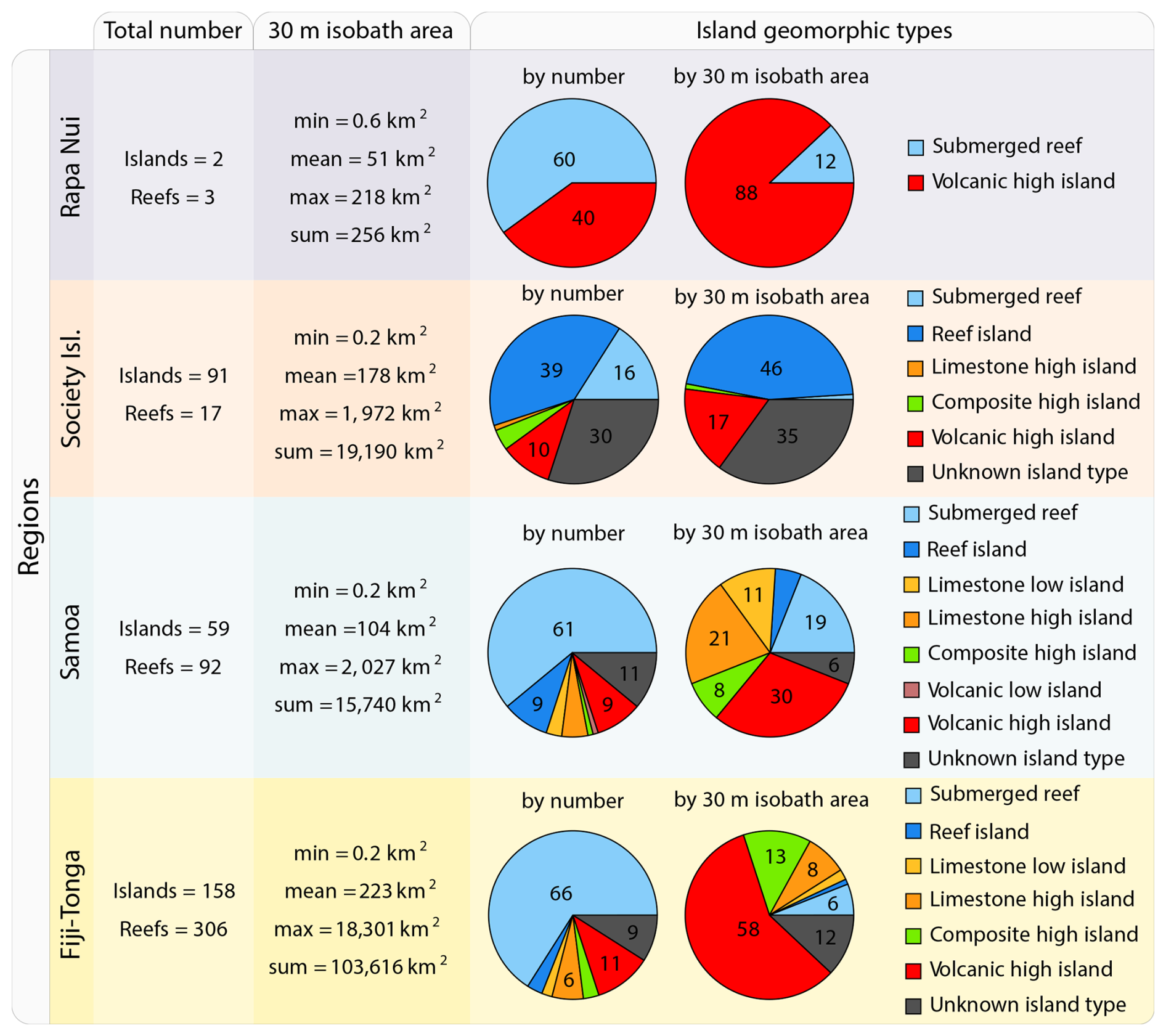
Figure 1 Island and submerged reef characteristics of the studied regions. Island geomorphic types were determined following Nunn et al. (2016).

2.2 In situ data collection

We measured inherent optical properties (IOPs), including absorption (a), attenuation (c), and backscattering (b_b), along the Tara Pacific transect, using Seabird's ACs spectrophotometer and ECO-BB3 integrated into a continuous flow-through system. We calculated particulate absorption (a_p), particulate attenuation (c_p), and particulate backscattering (b_bp) by correcting a, c, and b_b for instrument drift, bio-fouling, and the influence of dissolved matter, based on hourly measurements of 0.2 μm filtered seawater (Dall'Olmo et al., 2009; Slade et al., 2010; Boss et al., 2019). We derived bio-optical proxies for phytoplankton biomass and community composition from a_p and c_p, benefiting from the high sampling resolution of the continuous sampling system to detect gradients in optical properties along the sampling transect. We calculated the line-height of the a_p peak of [Chl a] at 676 nm (a_p676LH) (Boss et al., 2013) and decomposed all a_p spectra into Gaussian functions aligned with the light absorption peaks of specific accessory pigments (Chase et al., 2013). Each day, around 10:30 a.m. local time, we collected surface water samples for pigment analysis via high-pressure liquid chromatography (HPLC). We estimated [Chl a] from a_p by correlating total [Chl a] measured via HPLC with the amplitude of a_p676LH (Fig. A2). Similarly, we estimated accessory pigment concentrations from continuous underway measurements by relating concurrent pigment concentrations derived from HPLC to the amplitudes of a_p Gaussian functions (Fig. A2). Photo-protective carotenoid concentrations ([PPC]) were estimated from the Gaussian function centered on 492 nm, photosynthetic carotenoid concentrations ([PSC]) were estimated from the Gaussian function centered on 523 nm, chlorophyll c concentrations ([Chl c]) were estimated from the Gaussian function centered on 638 nm, and chlorophyll b concentrations ([Chl b]) were estimated from the Gaussian function centered on 660 nm (Table 1). We investigated changes in pigment composition along the Tara Pacific transect sampled using the ratio of these accessory pigments to [Chl a] (e.g. $\left[\text{PSC}\right]/\left[\mathrm{Chl}a\right]$; Table 1). Phycoerythrin concentrations were not measured as part of the HPLC analysis, thus we estimated the relative concentrations of phycoerythrin using the ratio of the Gaussian absorption function centered on the phycoerythrin absorption peak (i.e. 550 nm; Chase et al., 2013) to the Gaussian absorption function centered on 676 nm, the [Chl a] absorption peaks (i.e. $a_{\mathrm{gauss}}\mathrm{550}/a_{\mathrm{gauss}}\mathrm{676}$). Although not a central objective of this study, we tracked variations in ratios of these accessory pigments to [Chl a] (e.g. $\left[\mathrm{PSC}\right]/\left[\mathrm{Chl}a\right]$; Table 2) as a crude indicator of changes in phytoplankton community composition. To quantify changes in the mean size of suspended particles, we computed the slope exponent of c_p (i.e. ${\mathit{\gamma }}_{c_{\mathrm{p}}}$ which is inversely proportional to mean particle size; Boss et al., 2001). Additionally, we measured sea surface temperature and salinity (SSS) with a Seabird SBE45 thermo-salinograph integrated into the flow-through system. We also continuously recorded above-water instantaneous photosynthetically active radiation (iPAR) from the aft deck of Tara, using a cosine PAR sensor (QCP2150; Biospherical Instruments) positioned 5 m above sea level. All variables derived from in situ continuous underway data are described in Tables 1 and 2 and are publicly available (Bourdin and Boss, 2016). Finally, we collected daily discrete samples of surface seawater to estimate the concentrations of dissolved inorganic nitrogen (i.e., nitrates and nitrites), phosphate, silicate, and total iron (see sampling protocols in Lombard et al., 2023; Gorsky et al., 2019).

(Gardner et al., 2006; Behrenfeld and Boss, 2006)(Boss et al., 2001)(Kramer and Siegel, 2019)(Kramer and Siegel, 2019)(Kramer and Siegel, 2019)(Caferri et al., 2022)(Kramer and Siegel, 2019)(676 nm; Chase et al., 2013)

Table 1 Description of bio-optical proxies computed from in situ underway data.

(Geider et al., 1998)(e.g. lower light = higher $\mathrm{Chl}a/C_{\mathrm{phyto}}$; Geider et al., 1998)(higher Φ_Sat= higher stress; Behrenfeld et al., 2009)(Goes et al., 1999)

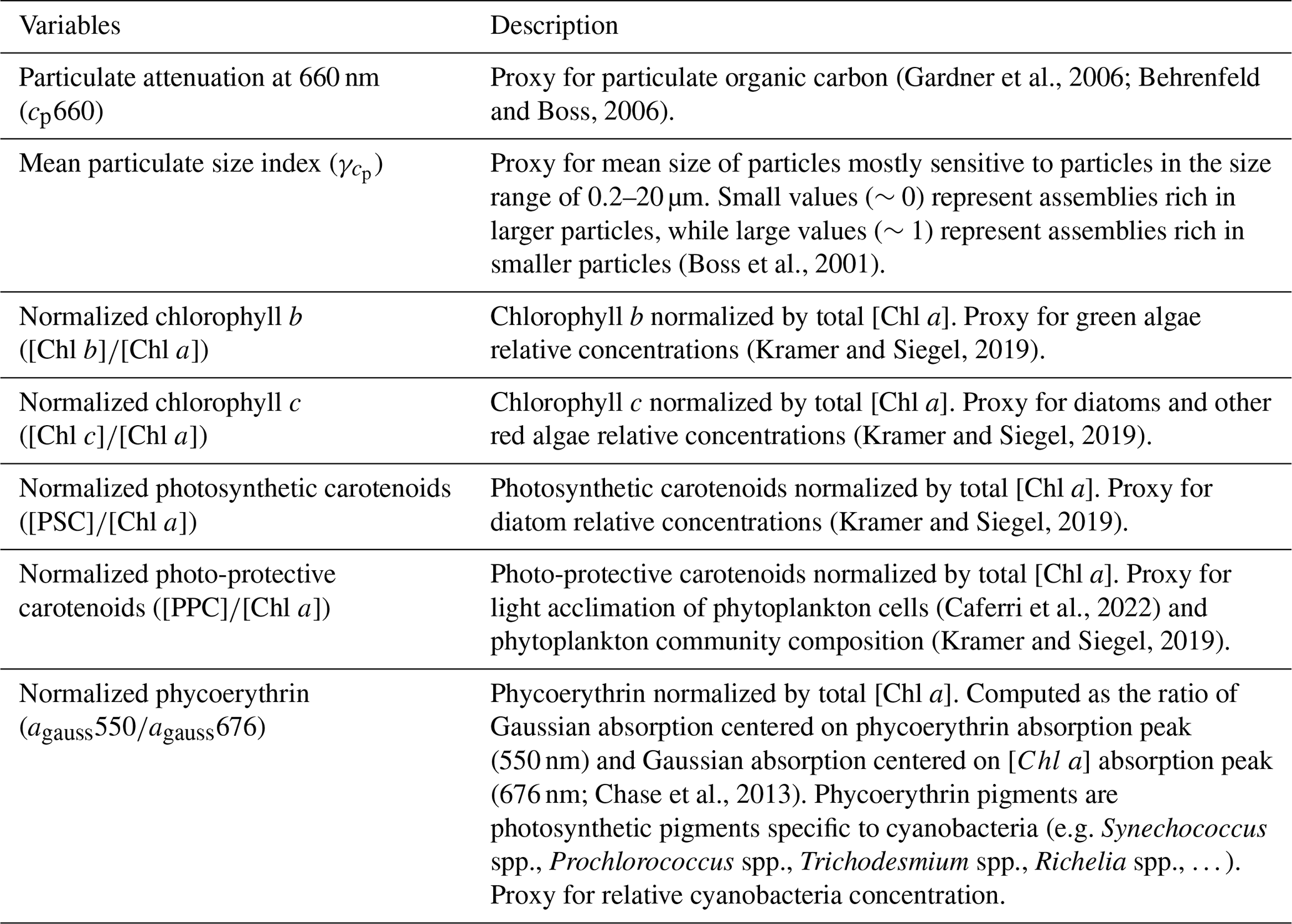
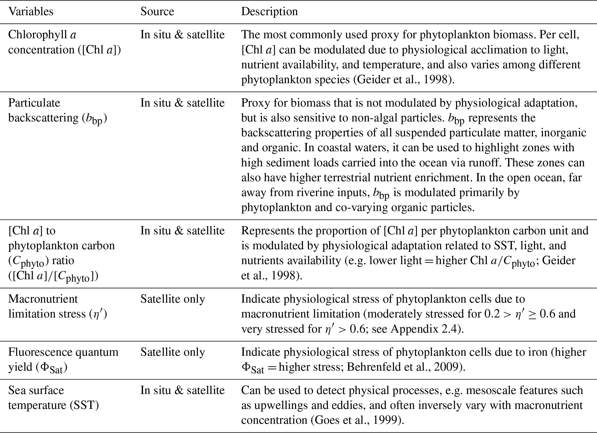
Table 2 Description of bio-optical and physical variables computed from in situ and satellite data.

2.3 Satellite products: phytoplankton biomass indicators

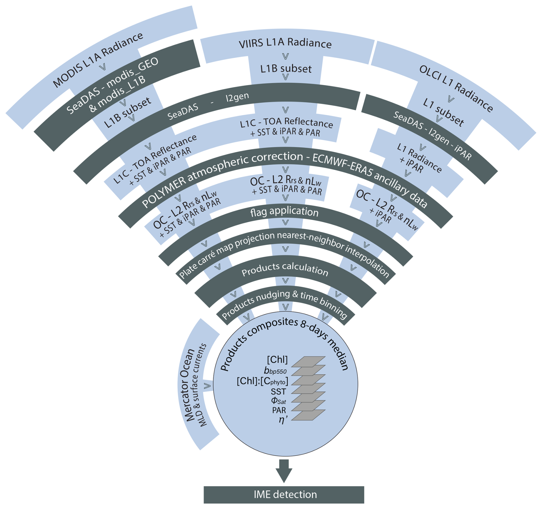
We computed level-2 (L2) satellite products from the Moderate Resolution Imaging Spectroradiometer (MODIS), the Visible Infrared Imaging Radiometer Suite (VIIRS), and the Ocean and Land Colour Imager (OLCI) level-1 data following Bourdin et al. (2025) method; we built two sets of satellite data, a “calibration dataset” and a “study dataset”. We downloaded the “calibration dataset” for the entire area covered by the Tara Pacific transect (May 2016 to October 2018, see Gorsky et al., 2019; Lombard et al., 2023). The “study dataset” consisted of four six-month-long sequences of satellite images in the vicinity of the islands of interest (see Sect. 2.5 for additional information on temporal coverage and resolution). We applied a polynomial-based atmospheric correction (POLYMER version v4.17beta2; Steinmetz et al., 2011; Steinmetz, 2023) on both datasets to compute 1 km spatial resolution L2 remote sensing reflectance data (R_rs) using ancillary data from the European Centre for Medium-Range Weather Forecasts reanalysis model version 5 (i.e. ERA5). We removed poor-quality data pixels by applying the flag recommendations of POLYMER (see reference POLYMER flags, 2024) and projected each satellite scene onto an equally spaced 1 km spatial resolution plate-carré reference grid using a nearest-neighbor interpolation from Python's SciPy library. We corrected R_rs for Raman scattering (Lee et al., 2013) and derived particulate back-scattering coefficient b_bp at 430 and 550 nm using the quasi-analytical algorithm V6 (Lee et al., 2002, 2009). We estimated [Chl a] using the blended CI-OCx algorithm applying the coefficients derived for each sensor (Hu et al., 2019; O'Reilly and Werdell, 2019). We estimated phytoplankton carbon (C_phyto) using the empirical relationship between b_bp(470 nm) and C_phyto (Graff et al., 2015). Following Bourdin et al. (2025), we computed surface-area integrated [Chl a] as a proxy for surface phytoplankton biomass integrated over entire IME and background ocean (BO) zones (see Sect. 2.6 for IME and BO zones definition), in two-dimensional metric tons of chlorophyll a (t m⁻¹), by summing the [Chl a] of each pixel within IME and BO zones multiplied by the area of that pixel:

$$\begin{array}{}\text{(1)}& \sum [\mathrm{Chl}a{]}_{\mathrm{IME}}=\sum _{n=\mathrm{1}}^{N_{{\mathrm{pixel}}_{\mathrm{IME}}}}[\mathrm{Chl}a{]}_n\times {\text{area}}_{{\mathrm{pixel}}_n}\end{array}$$

All variables derived from satellite data are described in Table 2.

2.4 Satellite products: phytoplankton physiological stress indicators

We computed two biomass-independent phytoplankton nutrient-stress indices. The fluorescence quantum yield (Φ_Sat) is indicative of the physiological stress of phytoplankton cells due to iron limitation (higher Φ_Sat = more iron stress) and was computed using intermediate products of [Chl a], normalized fluorescence line height (nFLH), and iPAR (Behrenfeld et al., 2009). iPAR was obtained from the output of the function l2gen of SeaDAS (Carder et al., 2003), and the computation of nFLH is detailed in Sect. A1 in the Appendix.

Huot et al. (2025) raised concerns about the limitations of using MODIS-Aqua data to compute Φ_Sat and infer phytoplankton iron stress. MODIS-Aqua overpass time (∼ 13:30 local at the equator) coincides with the time of the day when non-photochemical quenching (NPQ) is maximal, significantly reducing the signal-to-noise ratio of chlorophyll fluorescence after NPQ normalization (that is, FChl a_NPQ) and, consequently, Φ_Sat. In the present study, we also computed Φ_Sat from MODIS-Terra and OLCI Sentinel-3a, which sample the equator around 10 and 10:30 local time when the NPQ is likely different from the NPQ at the time of MODIS-Aqua overpass. Because the final product Φ_Sat is merged from MODIS-Aqua, MODIS-Terra, and OLCI Sentinel-3a, it benefits from an improved signal-to-noise ratio due to the combination of measurements taken at different times of the day. The quality of Φ_Sat computed here also benefited from the use of the POLYMER atmospheric correction scheme, which improves data retrieval around clouds and in sun-glint conditions. This is particularly important because the intermediate product of nFLH often shows artificially high values near clouds, likely due to the adjacency effect.

We derived a second physiological proxy that is indicative of phytoplankton stress due to macronutrient limitation. When incident light decreases, phytoplankton cells maintain their growth rate by upregulating chlorophyll pigment synthesis to compensate for the decreased solar energy available (Falkowski and Owens, 1980; Laws and Bannister, 1980). In contrast, phytoplankton cells under macronutrient stress downregulate chlorophyll pigments synthesis (Behrenfeld et al., 2015; Halsey and Jones, 2015; Laws and Bannister, 1980). The ratio of [Chl a] to C_phyto for a given growth irradiance represents the total physiological stress (${\mathit{\eta }}_{\mathrm{obs}}=\frac{\left[\mathrm{Chl}a\right]}{\left[C_{\mathrm{phyto}}\right]}$), and encompasses the physiological stress due to SST, light, and macronutrients availability (Geider et al., 1998; Halsey and Jones, 2015; Laws and Bannister, 1980). Although small changes in $\left[\mathrm{Chl}a\right]/\left[C_{\mathrm{phyto}}\right]$ have been attributed to temperature variations for a single species in ex situ experiments (Wang et al., 2009), it is likely that the species present in natural assemblages are adapted to their ambient temperature conditions. Given that SST is relatively homogeneous in this region on the timescale of physiological adaptation (i.e. a few days), we assume that all species are adapted to their ambient temperature conditions, making the impact of SST on $\left[\mathrm{Chl}a\right]/\left[C_{\mathrm{phyto}}\right]$ negligible at the community level. Consequently, we can isolate the physiological stress due to macronutrient limitation (η^′) by normalizing η_obs by the photoadaptation effect. As part of this process, we computed the median light in the mixed layer (I_ML) as follows:

$$\begin{array}{}\text{(2)}& I_{\mathrm{ML}}=\text{PAR}\times e^{-\mathrm{0.5}\times \text{MLD}\times {\mathrm{Kd}}_{\mathrm{PAR}}}\left[\mathrm{E}{\mathrm{m}}^{-\mathrm{2}}{\mathrm{d}}^{-\mathrm{1}}\right]\end{array}$$

where MLD is the mixed layer depth extracted from the Copernicus Marine Service Global Ocean Physics Reanalysis products (European Union-Copernicus Marine Service, 2019), PAR is the standard daily PAR output of the function l2gen of SeaDAS (Frouin and Pinker, 1995), and Kd_PAR is the diffuse attenuation coefficient of photosynthetically active radiance. Kd_PAR was approximated from the 1 % light horizon (Z_eu):

$$\begin{array}{}\text{(3)}& {\mathrm{Kd}}_{\mathrm{PAR}}=-{\displaystyle \frac{\ln \left(\mathrm{0.01}\right)}{Z_{\mathrm{eu}}}}\left[{\mathrm{m}}^{-\mathrm{1}}\right]\end{array}$$

where Z_eu is estimated from [Chl a] following Morel et al. (2007) Eq. (10):

$$\begin{array}{}\text{(4)}& {\log }_{\mathrm{10}}{Z}_{\mathrm{eu}}=\mathrm{1.524}-\mathrm{0.436}X-\mathrm{0.0145}{X}^{\mathrm{2}}+\mathrm{0.0186}{X}^{\mathrm{3}}\left[\mathrm{m}\right]\end{array}$$

with X=log ₁₀[Chl a]. We partitioned all I_ML and η_obs of the four case study regions into two-dimensional bins spanning the entire dynamic range of I_ML and η_obs of the entire dataset. Because the quantity of level-2 data is too large for our computing capacity, we used 8 d medians merged products of all variables used in this computation (see merging method Sect. 2.5). We identified the 1^st and 95^th percentiles of η_obs for each I_ML bin to which we fitted a simple exponential model (Fig. 2):

$$\begin{array}{}\text{(5)}& {\widehat{\mathit{\eta }}}_{\mathrm{obs}}=A+B\times {\exp }^{-C\times I_{\mathrm{ML}}}\end{array}$$

The model equations fitted on the 1st and 95th percentiles of η_obs represent the range of acclimation for the entire dataset.

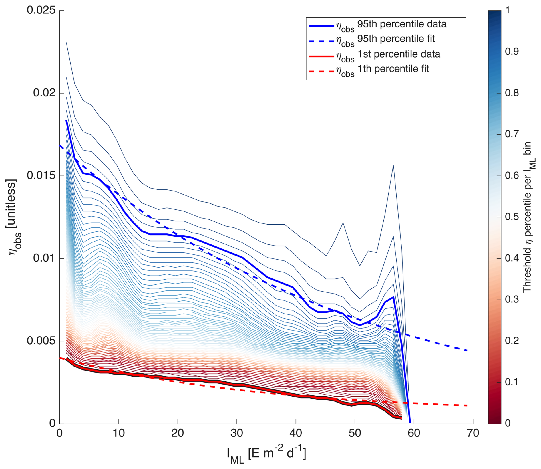
Figure 2 Percentiles of η_obs per I_ML bins. The blue and red solid lines highlight the 95th and 1st percentiles in each I_ML bin. The dashed lines represent the equations Eq. (5) fitted on them.

For each pixel, we computed the difference between the macronutrient replete state ($\widehat{{\mathit{\eta }}_{{\mathrm{obs}}_{\max }}}$) and the observed state η_obs relative to the full span of η for the pixel's given I_ML to provide a quantitative metric of the degree of macronutrient stress:

$$\begin{array}{}\text{(6)}& {\mathit{\eta }}^{\prime }={\displaystyle \frac{\widehat{{\mathit{\eta }}_{{\mathrm{obs}}_{\max }}}-{\mathit{\eta }}_{\mathrm{obs}}}{\widehat{{\mathit{\eta }}_{{\mathrm{obs}}_{\max }}}-\widehat{{\mathit{\eta }}_{{\mathrm{obs}}_{\min }}}}}\left[\text{unitless}\right]\end{array}$$

Thus, η^′ is scaled to the parameter space of the specific remote sensing dataset used for this study, and is representative of the relative nutrient stress in the studied regions over the 6-month time series. We arbitrarily defined three macronutrient stress categories, classifying phytoplankton populations as macronutrient-replete when ${\mathit{\eta }}^{\prime }\le \mathrm{0.2}$ (including negative values), moderately stressed when $\mathrm{0.2}<{\mathit{\eta }}^{\prime }\le \mathrm{0.6}$, and highly stressed when ${\mathit{\eta }}^{\prime }>\mathrm{0.6}$.

2.5 Satellites products adjustment and merging

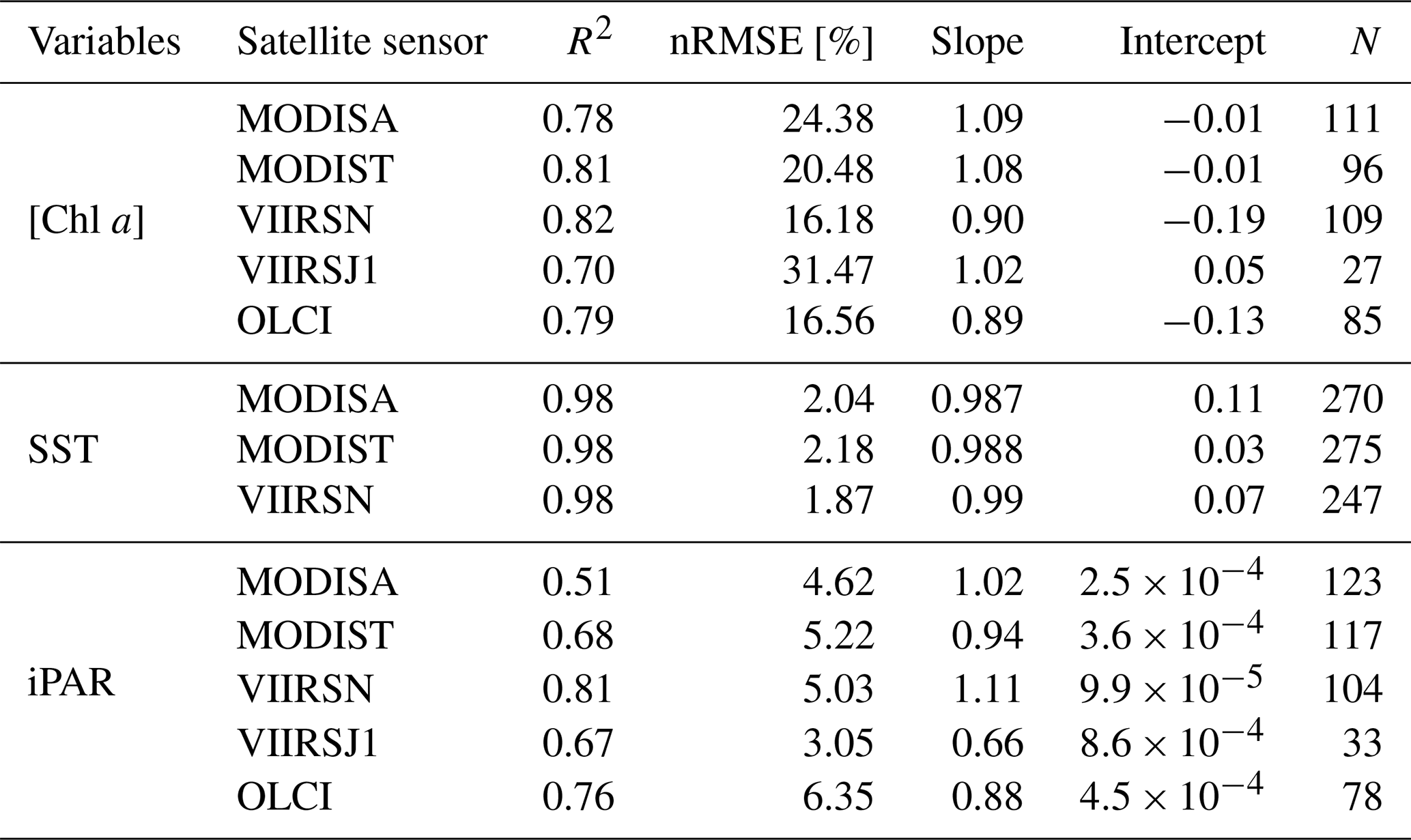
Level-2 satellite estimates of SST, [Chl a], and iPAR (different from the daily PAR used in η^′ computation) were individually calibrated against in situ measurements obtained from the underway system of the ship to minimize inter-sensor variability and biases. We performed match-ups and robust linear regressions between these variables measured in situ and their satellite counterparts derived from the calibration dataset (Appendix A2). We used the parameters from their respective robust linear regressions (see Table A1) to produce “calibrated” products before merging them. For parameters derived from remote sensing data with no comparable in situ measurements (e.g. Φ_Sat), we adjusted the values from all sensors to align with those of MODIS-Aqua, minimizing inter-sensor discrepancies. This alternative method improved the smoothness of the final merged product and the delineation of spatial patterns. However, potential biases associated with the retrieval of products not calibrated against in situ data remained unconstrained. Although in situ b_bp data were available, the relation between in situ b_bp and satellite b_bp was very sensitive to match-up criteria, and the linear regressions were not well constrained (see Appendix A4). The coefficients used to align the data from different satellite sensors with in situ b_bp were inaccurate, leading to noisy merged satellite b_bp products. Moreover, an artifact was discovered in MODISA and MODIST b_bp maps in ultra-oligotrophic regions ([Chl a]<0.04 mg m⁻³; see Appendices A3 and A4). Therefore, only OLCI and VIIRS-SNPP b_bp were binned into the 8 d median products, and OLCI was nudged to best match VIIRS-SNPP's values. We performed this cross-satellite sensor nudging only when: (1) at least 10 % of the total pixels of the adjusted sensor and the reference sensor were valid (i.e. unflagged), (2) the slope of the fit was positive, (3) R²≥0.9, and (4) nRMSE ≤10 %. Before computing the merged products of a given 8 d period and a given region, we grouped all re-projected level-2 images and removed outliers based on the distribution of all individual measurements of the grouped scenes (following the same outlier removal method as in Bourdin et al., 2025, Appendix C). For each case study presented here, we produced a 6-month-long time series of 8 d medians of each of the variables presented in Table 2 (i.e. Animations S1, S2, S3, and S4 in the Supplement), following the approach of Bourdin et al. (2025). Each case study region was centered geographically on an island sampled during the Tara Pacific expedition (Fig. 3), and each 6-month time series was centered temporally on the day of in situ sampling by Tara (Gorsky et al., 2019; Lombard et al., 2023). We propagated the error associated with the satellite product retrieval, nudging, and merging throughout each step to represent the final binned product uncertainty denoted as the standard error of mean (i.e. SEM) of the merged product (e.g. ${\text{SEM}}_{[{\mathrm{\Phi }}_{\mathrm{Sat}}{]}_{\mathrm{IME}}}^{\mathrm{f}}$; see Appendix A4). We used this final uncertainty to determine if changes associated with an IME are significant.

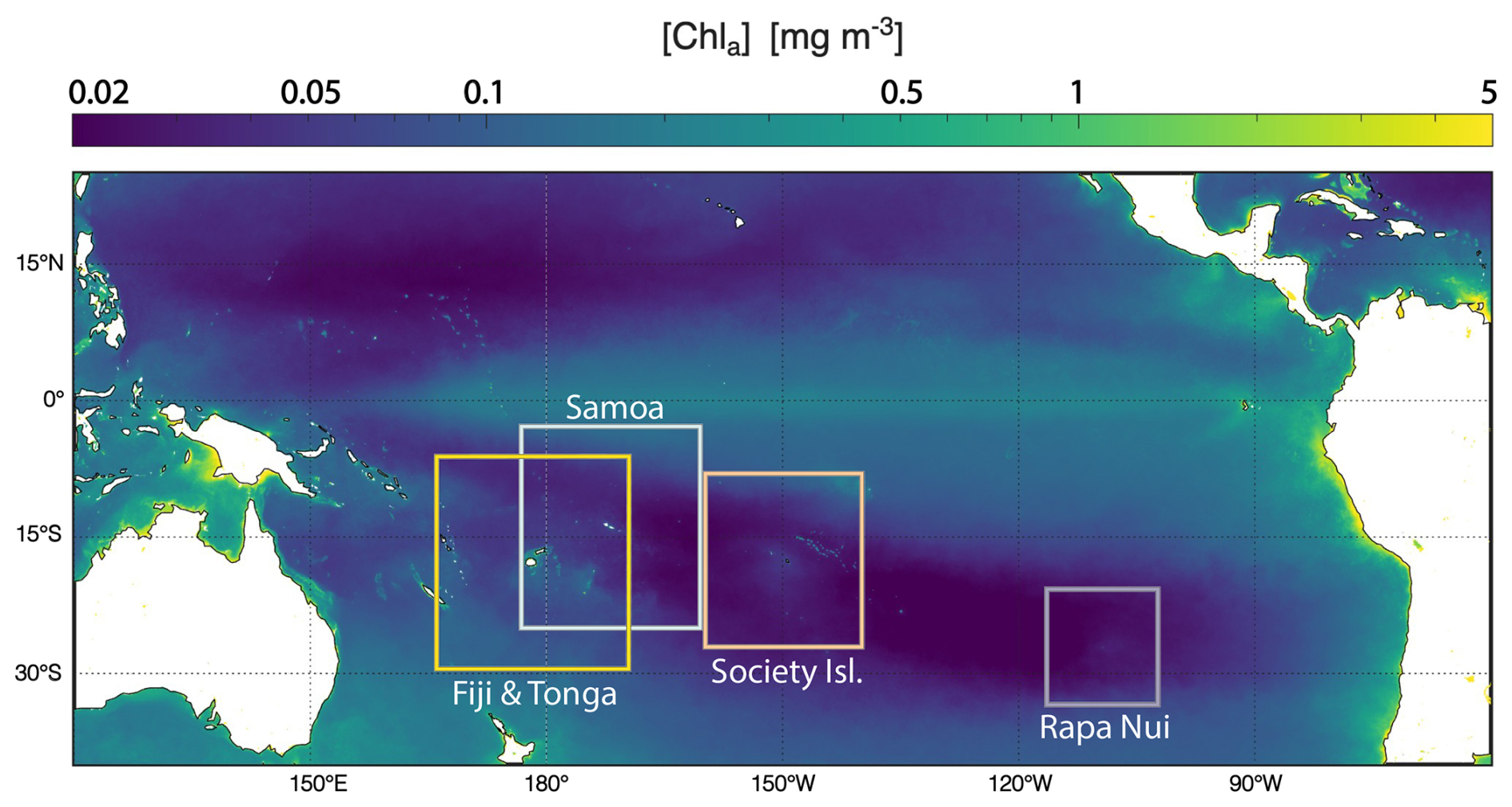
Figure 3 Average of MODIS-Aqua monthly chlorophyll a concentration over the entire study period (1 June 2016–30 September 2017) and region, overlaid with the area covered by the binned map of each studied archipelago.

2.6 Island Mass Effect Detection

We detected IMEs on each 8 d median map using an iterative method to define a [Chl a] contour around each individual IME (see method in Bourdin et al., 2025). We used the islands and submerged reefs database from Bourdin et al. (2025), which was consolidated from the General Bathymetric Chart of the Oceans (GEBCO) database (GEBCO Bathymetric Compilation Group, 2022), the high-resolution global island database (Sayre et al., 2019, 2020), and the submerged reef database from Messié et al. (2022). Following the methodology in Messié et al. (2022) and Bourdin et al. (2025), submerged topographic features shallower than 30 m depth are treated as islands in the IME detection algorithm; therefore, the term IME can also be used in this study to qualify enhanced [Chl a] zones associated with seamounts. We used the modeled daily surface currents data for the detection algorithm (i.e. global ocean ensemble physics reanalysis products distributed by Copernicus Marine Services; European Union-Copernicus Marine Service, 2019). As in previous studies (Messié et al., 2022; Bourdin et al., 2025), we define the background ocean (BO) reference zone associated with each IME zone as an area equal in size to the corresponding IME zone but located outside of it, closest to the island or submerged reef mask. We focused our analysis on archipelagos located near the center of each study region. We excluded IMEs detected near regional domain boundaries from the analysis because one of the stopping criteria of the detection algorithm could be triggered prematurely near the domain boundaries, thus underestimating the area of that IME (Bourdin et al., 2025). Large IME patches – such as those associated with the Society Islands, Samoa, and Fiji – frequently stem from the combined effects of multiple islands, each of which may generate its own local IME superimposed on the broader signal of the main island (Bourdin et al., 2025). To account for this, we identified all islands that were included at least once within the IME associated with each main archipelago during the analyzed 6-month period and selected all IME events linked to this set of islands for each region. Using this approach, we detected a total of 2025 individual IME realizations associated with the four studied archipelagos over the six-month study periods. We then extracted bio-optical properties derived from satellite data for all these 2025 IMEs and their associated BO areas. To identify consistent patterns across the South Pacific Subtropical Basin and all seasons sampled, we performed a principal component analysis (PCA) using the average bio-optical properties of all the 2025 individual IME realizations detected and their associated BO areas. Only variables derived from satellite measurements and assimilative models were used in this analysis to ensure sufficient data coverage (i.e. [Chl a], b_bp, $\left[\mathrm{Chl}a\right]/\left[C_{\mathrm{phyto}}\right]$, SST, MLD, Φ_Sat, and η^′). Additionally, we identified in situ measurements located within IMEs contours to validate patterns we observed in satellite data and complement the interpretation with information on pigment ratios as proxies for phytoplankton community composition, as well as macronutrient and iron concentrations. To examine the differences between coastal IMEs and advected IMEs, we categorized all in situ observations (i.e. continuous underway measurements, macronutrient concentrations, and iron concentrations) into three groups: background ocean (BO), coastal IME, and advected IME. In situ data located within an IME contour detected from satellite observations and over bathymetry shallower than 100 m were classified as coastal IME, whereas all remaining in situ data within IME contours were classified as advected IME (see Appendix B). We limited this categorization to in situ data because satellite data in shallow areas are, in general, not retrieved in clear water conditions due to the impact of bottom reflectance on radiometric estimates.

3 Results and Discussion

Six-month-long time-series data highlighted relatively strong seasonal variability in IME magnitude (Bourdin et al., 2025), but also showed consistent contrasts between properties of IME and BO zones across the longitudinal gradient. IMEs associated with the studied islands were consistently characterized by higher average $\left[\mathrm{Chl}a\right]/\left[C_{\mathrm{phyto}}\right]$, and lower averages of Φ_Sat and η^′ relative to BO (Figs. 4 and B1). These results are consistent with the hypothesis that IMEs are areas where nutrient limitation is alleviated compared to the background ocean.

In each region studied, the difference between the IME and BO centroids is aligned with the vector of Φ_Sat and is larger in the western basin (i.e. Samoa, and Fiji and Tonga case studies) than in the eastern basin of the SPSG (i.e. Rapa Nui and Society Islands case studies; Figs. 4 and B1), suggesting that iron enrichment in IME zones is higher in the western Pacific compared to the eastern basin. This difference may be due to higher concentration of active shallow and deep hydrothermal vents located around islands and seamounts in the western Pacific basin, which serve as substantial sources of iron in this region (Bonnet et al., 2023; Guieu et al., 2018). Another key oceanographic difference between the eastern and western SPSG is the depth of the nutricline, which is generally deeper in the east, particularly around Rapa Nui (∼150–220 m in the eastern basin versus 70–80 m in the western basin; Longhurst, 2007; Raimbault et al., 2008). Consequently, wind-driven divergence in the eastern basin is more likely to upwell nutrient-depleted water from above the nutricline. In addition, for a given wind speed, the magnitude of upwelling and macronutrient enrichment is expected to be stronger around large islands with long and continuous coastlines, such as Viti Levu in the Fiji archipelago, than around isolated small islands like Rapa Nui or archipelagos of smaller islands such as the Society Islands (De Falco et al., 2022).

The Society Islands, Samoa, and Fiji-Tonga IMEs were characterized by reduced η^′ relative to their respective BO zones (Fig. 4). Two phases of IME occurred around Rapa Nui. The first phase, the austral winter phase, was characterized by higher vertical mixing (i.e. deeper MLD), lower SST, and no apparent correlation of the IME with η^′ (i.e. circles located at the top part of the scatter plot). The second phase, the austral summer phase, was characterized by shallower MLD, higher SST, and correlations between IME and lower macronutrient stress (i.e. circles located in the middle of the scatter plot). The points corresponding to the austral winter phase are distinct from the austral summer phase, and exhibit similar properties to the Society Islands' IME (Fig. 4). Rapa Nui is located 10° S of Tahiti, just at the border of a strong SST latitudinal gradient visible south of Rapa Nui in the video supplements (or at Bourdin, 2025), suggesting that Rapa Nui's IME is characterized by different water mass properties than Tahiti during the austral winter.

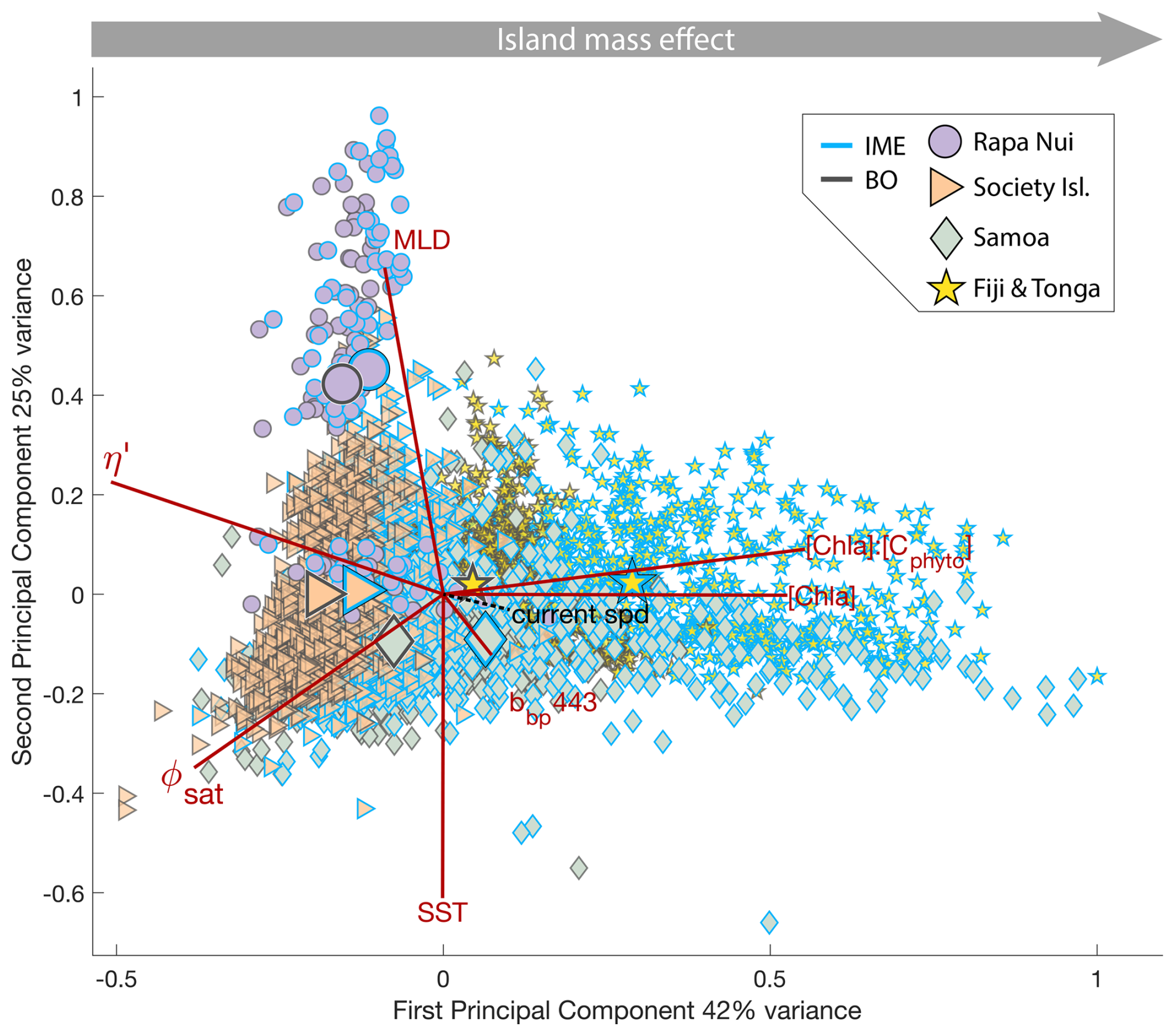
Figure 4 Principal component analysis of average chlorophyll a concentration ([Chl a]), backscattering coefficient at 443 nm (b_bp443), ratio of [Chl a] to phytoplankton carbon ($\left[\mathrm{Chl}a\right]/\left[C_{\mathrm{phyto}}\right]$), iron stress index (Φ_Sat; iron stress index), macronutrient stress index (η^′), mixed layer depth (MLD), and sea surface temperature (SST) of all individual IME (blue outline) and background ocean (BO, black outline) zones detected in each 8 d period along the six-month time-series in all of the four case studies (N=2025 realizations of IMEs). Small markers represent all individual IME and BO averages for each studied region, and larger markers represent their centroids. Surface current speed (“current spd”) is overlaid in black as a supplementary variable.

All IMEs, were characterized by moderate increases in b_bp at 443 nm (b_bp443) and therefore increases in phytoplankton biomass (Figs. 4 and B1). The detected increase in b_bp in the eastern basin (Rapa Nui and Society Isl.) is only marginal but measurements from the continuous underway system show higher surface c_p660 values within all IME zones across the four case studies (Bourdin et al., 2025). Assuming in situ sampling periods are representative of the six-month time-series, the increases in biomass associated with IMEs in the eastern basin were likely close to the detection limit of b_bp via satellite (due to high uncertainty in retrieval, see Sect. A3, Bisson et al., 2021). The ultra-oligotrophic ocean in the eastern basin is largely dominated by picophytoplankton that are tightly coupled with their grazers, heterotrophic and pigmented nanoflagellates, which have similar generation times on the order of a day (Connell et al., 2020; Livanou et al., 2019; Yun-Chi et al., 2009). This tight coupling may have prevented an accumulation of phytoplankton biomass detectable from remote sensing in this region.

In order to investigate the sources of nutrients associated with IME, we analyze incoming and outgoing transects around islands to identify markers of upwelling of deep nutrient-rich water to the surface. We also examined these transects to identify zones of minimum macronutrient or iron stresses corresponding to zones of higher biomass, macronutrient, and iron concentrations, which would inform on the origin of enrichments.

3.1 IME and phytoplankton photophysiology

The IME detected around Fiji was characterized by a surface integrated [Chl a] enhancement of about 55 t m⁻¹ and covered a surface of about 500 000 km² at the time of sampling (Bourdin et al., 2025). The increase of c_p660 (i.e. proxy for particulate organic carbon concentration; see Table 1) by a factor of ∼15 observed over a ∼10 km transect approaching shore, west of the archipelago, suggests the [Chl a] enhancement in the IME was associated with a significant increase in phytoplankton biomass (Fig. 6 in Bourdin et al., 2025). A distinct and synchronized decrease in SST and increase in SSS on 30 May ∼10:00 UTC indicated a change in seawater physical properties measured along the inbound transect to the Fiji archipelago (Fig. 5B and C). This change in water mass physical properties was associated with a gradual decrease in the proportion of photoprotective carotenoids ($\left[\mathrm{PPC}\right]/\left[\mathrm{Chl}a\right]$) and a gradual increase in $\left[\mathrm{Chl}a\right]/\left[C_{\mathrm{phyto}}\right]$ (Fig. 5D and E). These two independent metrics of light acclimation had opposite trends, suggesting that the same forcing was impacting both of them. The proportion of [PPC] can be modulated by phytoplankton in response to changes in ambient light to prevent intracellular photo-oxidative stress (Caferri et al., 2022). Likewise, the proportion [Chl a] to [C_phyto] is modulated in response to light conditions, resulting in phytoplankton cells at the surface of the ocean characterized by lower $\left[\mathrm{Chl}a\right]/\left[C_{\mathrm{phyto}}\right]$ and higher $\left[\mathrm{PPC}\right]/\left[\mathrm{Chl}a\right]$ than cells residing at depth, where low levels of ambient light require more [Chl a] for photosynthesis but also cause less photo-oxidative stress, therefore requiring lower concentrations of photoprotective pigments. The lowest SST and $\left[\mathrm{PPC}\right]/\left[\mathrm{Chl}a\right]$ and the highest $\left[\mathrm{Chl}a\right]/\left[C_{\mathrm{phyto}}\right]$ of the inbound transect were measured just adjacent to the island's shelf break. These parameters changed suddenly when Tara sailed across the shelf through the Navula Passage west of the Fiji archipelago (i.e. coastal zone Fig. 5D and E). Together, these synchronized trends observed with four independent measurements suggest an upward entrainment of water parcels and low-light adapted phytoplankton cells, an observation that is consistent with the occurrence of an upwelling event. Based on the spatial variability of these parameters, we estimate that this upwelling occurred in a ∼170 km wide band adjacent to the island shelf west of Viti Levu at the time of sampling. $\left[\mathrm{PPC}\right]/\left[\mathrm{Chl}a\right]$ was marginally lower, and $\left[\mathrm{Chl}a\right]/\left[C_{\mathrm{phyto}}\right]$ was marginally higher, but overall heterogeneous in this IME detected in the outbound transect, suggesting a weaker upwelling of cells that are acclimated to low light to the surface than in the inbound transect. The surface currents were flowing southward at the time of sampling and the week before, suggesting that the IME detected south of Fiji was located downstream of Fiji. The inbound transect to Fiji crossed an IME episode associated with a submerged seamount located north of Fiji and not connected to the island shelf (15°39^′38.2^′′ S, 175°51^′59.8^′′ E; the IME is visible in the inbound panel of Fig. 5 but is outside the domain of the zoomed maps in Fig. 6). This IME episode was also characterized by a synchronized decrease in $\left[\mathrm{PPC}\right]/\left[\mathrm{Chl}a\right]$ and an increase in $\left[\mathrm{Chl}a\right]/\left[C_{\mathrm{phyto}}\right]$, consistent with the entrainment of low-light-adapted phytoplankton into the surface layer. This pattern suggests enhanced vertical mixing around the seamount, likely driven by the interaction between ambient currents and the seamount topography (Lueck and Mudge, 1997; Wang et al., 2024; Dai et al., 2020; Leitner et al., 2020). Similar signals were detected southwest of Rapa Nui and Tahiti-Mo'orea, along the outbound transects, indicating that sub-surface phytoplankton populations were recently upwelled to the surface (see Appendix B). In contrast, there is no clear evidence that upwelling occurred around Samoa at the time of sampling (see Appendix B). Indeed, in situ data show that the IME advected offshore had the same characteristics as the water mass closest to shore (that is, higher SST, lower SSS, and no significant differences in $\left[\mathrm{PPC}\right]/\left[\mathrm{Chl}a\right]$ and $\left[\mathrm{Chl}a\right]/\left[C_{\mathrm{phyto}}\right]$; see Appendix B), therefore the main source of nutrient in Samoa's IME were likely associated with terrigenous processes.

We extracted satellite estimates of [Chl a], $\left[\mathrm{Chl}a\right]/\left[C_{\mathrm{phyto}}\right]$, and SST along the ship track (i.e. dashed line Fig. 5) to assess if satellite-based estimates can also inform us about processes involved in IME. Although satellite-derived [Chl a] and SST closely matched the magnitude of in situ underway measurements, the satellite $\left[\mathrm{Chl}a\right]/\left[C_{\mathrm{phyto}}\right]$ values along the ship track were consistently lower than those estimated from in situ underway data. Satellite [Chl a] and SST were nudged to agree with in situ underway estimates across the Pacific Ocean (see Sect. 2.5 and Bourdin et al., 2025), however, bbp was not adjusted because of the low correlation between in situ and satellite data (see Sect. 2.5). This suggests that the Quasi-Analytical Algorithm (QAA; Lee et al., 2002, 2009) we used to invert b_bp from R_rs may not perform well in these ultra-oligotrophic regions since all b_bp measurements used to develop this inversion algorithm are higher than the in situ b_bp of the BO zones we measured in these regions (b_bp443<0.001 m⁻¹). Moreover, b_bp inverted from satellite data using QAA was shown to be overestimated in these regions when compared to b_bp estimated from profiling floats (when b_bp700<0.001 m⁻¹; Bisson et al., 2021). In this case, an overestimation of the satellite b_bp would lead to an underestimation of $\left[\mathrm{Chl}a\right]/\left[C_{\mathrm{phyto}}\right]$ and would explain the observed discrepancies between in situ and satellite estimates. Despite this difference in magnitude, the spatial variability of $\left[\mathrm{Chl}a\right]/\left[C_{\mathrm{phyto}}\right]$ estimated from satellite data captured the same spatial variability as the situ estimates, although slightly smoother due to the 8 d time binning applied (i.e. dashed line Fig. 5). These results show the potential of satellite data to discriminate between biomass enhancement and signatures of coastal upwellings around islands and improve the mechanistic understanding of IME. However, it requires minimizing the satellite temporal binning to capture short-lived events that would otherwise be undetectable.

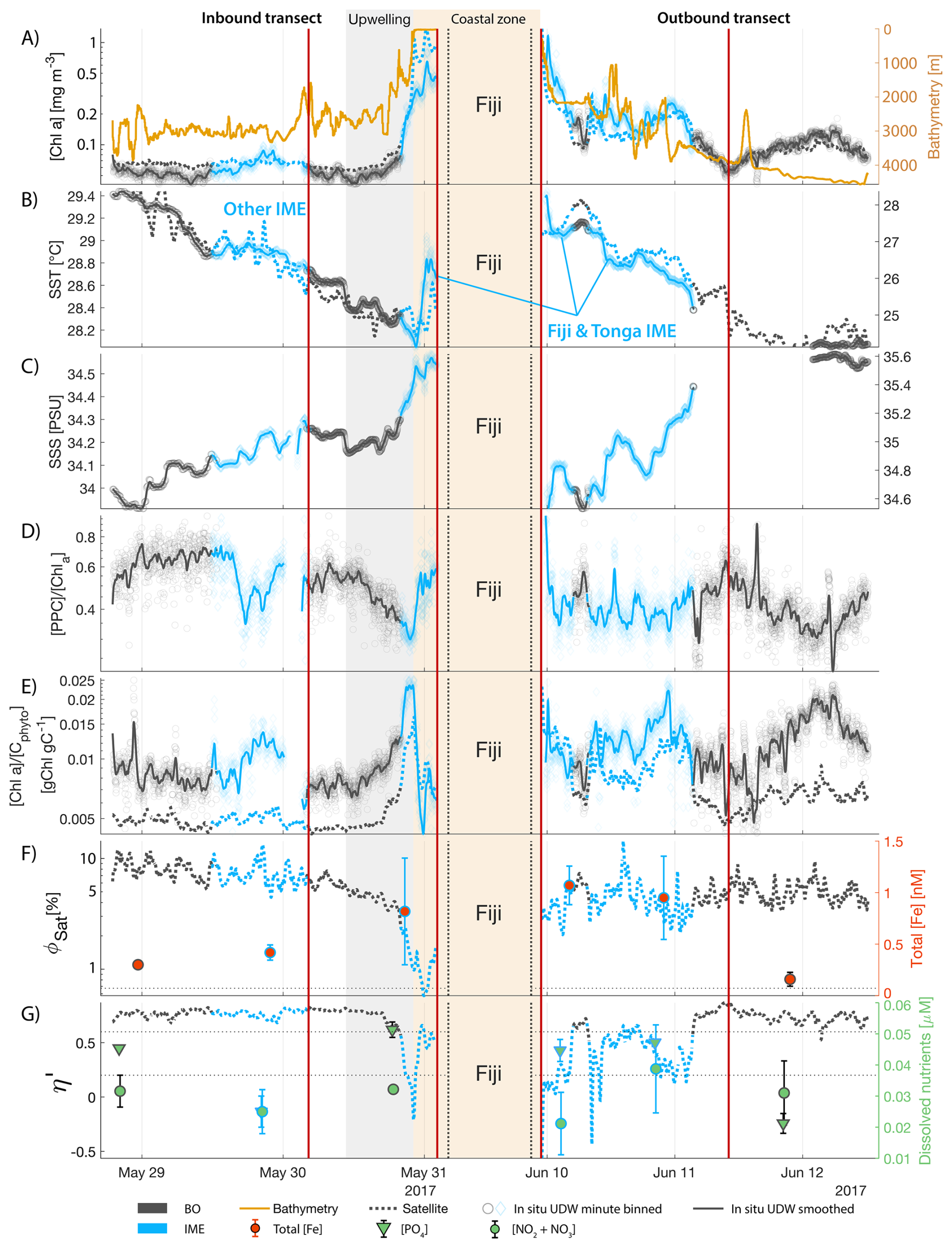
Figure 5 Underway data measured during the inbound (left panels) and outbound (right panels) transects around Fiji and their satellite counterparts, when available. (A) Chlorophyll a concentration ([Chl a]) and bathymetry, (B) sea surface temperature (SST), (C) sea surface salinity (SSS), (D) Photo-protective carotenoids proportion ($\left[\mathrm{PPC}\right]/\left[\mathrm{Chl}a\right]$; indicative of phytoplankton light acclimation), (E) [Chl a] to phytoplankton carbon ratio ($\left[\mathrm{Chl}a\right]/\left[C_{\mathrm{phyto}}\right]$), (F) fluorescence quantum yield (Φ_Sat; iron stress index) and total iron concentration measured at sampling stations, and (G) macronutrient stress index (η^′) and macronutrient concentrations measured at sampling stations. The blue points show in situ data falling in IME zones detected on the overlapping 8 d satellite composite (BO = black circle, IME = blue diamond). The points show the minute-binned underway data, and the solid lines represent the underway data smoothed with a 2 h low-pass digital filter. The gray shaded area highlights the coastal upwelling zone, and the beige shaded area highlights the transect over shallow waters (<100 m depth). The red vertical lines represent the start and end times of the inbound and outbound transect sections shown in Fig. 6.

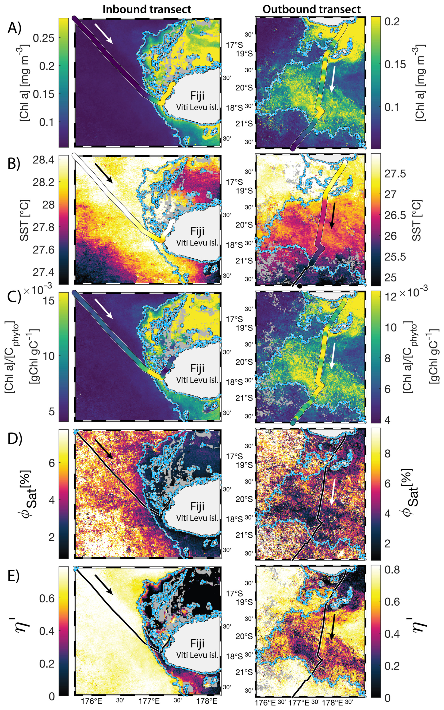
Figure 6 8 d median satellite maps zoomed on the inbound (left-hand-side panels) and outbound transects (right-hand-side panels) around Fiji (arrow shows sailing direction). The blue contour delineates the island mass effect zone detected from satellite chlorophyll a concentration ([Chl a]). In situ underway measurements are overlaid on the satellite map if the same variable was measured from satellite estimates and the underway system. (A) [Chl a], (B) sea surface temperature (SST), (C) [Chl a] to phytoplankton carbon ratio ($\left[\mathrm{Chl}a\right]/\left[C_{\mathrm{phyto}}\right]$), (D) fluorescence quantum yield (ϕ_Sat; iron stress index), and (E) macronutrient stress index (η^′). Entire six-month animated time series accessible in video supplements (Animation S1 in the Supplement).

3.2 IMEs and spatial pattern in phytoplankton nutrient physiology

The satellite map around Fiji shows that the IME patch is characterized by higher $\left[\mathrm{Chl}a\right]/\left[C_{\mathrm{phyto}}\right]$, as well as lower Φ_Sat and η^′ indices, suggesting enrichment in iron and macronutrients, and enhanced upwelling of subsurface phytoplankton population within the IME relative to BO (Figs. 6 and 5). Total iron concentrations measured at the sampling stations were the highest in Fiji's IME (Fig. 5). The iron stress index (Φ_Sat) decreased along the inbound transect, with the steeper decrease detected over the island shelf, past the detected upwelling zone. This suggests that iron enrichment was driven by processes associated with the archipelago itself (e.g. leaching from sediments, runoff, or shallow hydrothermal activity) rather than the upwelling event (Fig. 5). The macronutrient stress index (η^′) also decreased along the inbound transect with a minimum coinciding with the upwelling signal and higher values over the shelf area, suggesting that the upwelling west of Fiji was an important source of macronutrients to the euphotic zone further away from shore. η^′ was also consistently lower in the entire IME zone relative to the BO, with lower values detected as far as ∼150 km offshore on the outbound transect, suggesting a macronutrient enrichment across Fiji-Tonga's IME. Differences in spatial variability between macronutrient or iron concentrations and their respective stress indices can result from two (or more) factors. (1) Macronutrient and iron concentrations reflect standing stocks, whereas the stress indices are more indicative of the macronutrient and iron fluxes experienced by cells. In other words, although high macronutrient and trace metal concentrations likely imply increased supply, low concentrations do not necessarily imply limiting flux. (2) The spatial resolution of sampling differs between measurement types: the macronutrient and iron stress indices (respectively η^′ and Φ_sat) are retrieved at 1 km² resolution, while discrete sampling of macronutrients and iron were collected at a much coarser spatial resolution (on average every 290 km). Despite these differences, the combined use of both concentrations and stress indices is informative because a disparity between them is suggestive of rapid uptake of macronutrients or iron by local phytoplankton populations.

The concentrations of nitrogen and phosphate were, in general, higher at coastal stations compared to offshore stations (advected IME and BO; Fig. C1), indicating that terrigenous inputs, through runoff and organic macronutrient production in coral reefs, were a significant source of macronutrients close to shore. These concentrations were rarely higher in the advected IME compared to the BO. For example, despite a strong enrichment in nitrogen and phosphate in the coastal IME of Fiji (Fig. C1), concentrations are already low at the closest station to the island shore downstream of Fiji (Fig. 5), suggesting that a large proportion of these macronutrients were rapidly depleted relatively close to shore. The upstream water masses, which were impacted by local coastal upwelling and terrigenous processes, were probably diluted south of Fiji through mixing with the oligotrophic BO and modified by local upwelling and downwelling associated with positive and negative vorticity (De Falco et al., 2022). Interactions of currents with islands and seamount topography can also result in doming isopycnals and increased vertical mixing downstream of islands (Heywood et al., 1990; De Falco et al., 2022). This enhanced vertical mixing could have sustained a small influx of macronutrients to the euphotic zone in the IME, as shown by the consistently lower macronutrient stress (i.e. ${\mathit{\eta }}^{\prime }\le \mathrm{0.6}$) in the IME zone of the outbound transect. Although phosphate concentrations measured at stations located in the IME of Fiji-Tonga were consistently higher than in the BO, nitrogen concentrations were lower at the offshore station closest to Fiji on the outbound transect (Fig. 5). Phytoplankton biomass was higher at this station, particles were larger on average (lower γ_cp), and pigment ratios were characteristic of a higher proportion of diatoms (higher $\left[\mathrm{PSC}\right]/\left[\mathrm{Chl}a\right]$), suggesting that nitrogen (nitrate + nitrites) could have been quickly consumed by the phytoplankton community (Figs. B6 and 7).

Relatively high total iron concentrations were detected downstream of Fiji (south), further away from the coast, yet Φ_Sat increased rapidly along the outbound transect. Automated microscopy analyses show a high prevalence of Trichodesmium spp. in the IME zone along the outbound transect (Mériguet et al., 2024, 2025), and this bloom was visible to the naked eye during sampling (Bourdin, personal observation). Iron requirements vary between phytoplankton taxa; for example, Trichodesmium spp. is known to have higher iron requirements compared to other taxa (Berman-Frank et al., 2001a). Furthermore, there is a high inter-species variability in the ratio of chlorophyll fluorescence to chlorophyll concentration (i.e. FChl $/$ [Chl a]) (Petit et al., 2022; Roesler et al., 2017), which could impact the estimation of Φ_Sat and explain the difference in the relationship between the total iron concentration and Φ_Sat at these stations. Trichodesmium spp. colonies are composed of “bright cells” that have twice the basal fluorescence of other cells in a non-diazotrophy state and three times as many when in a diazotrophy state (Berman-Frank et al., 2001b; Küpper et al., 2008). The bloom of Trichodesmium spp. observed on the outbound transect at sampling stations where the total iron concentration was an order of magnitude higher than in BO indicates that diazotrophy was likely occurring in this bloom. Trichodesmium spp. diazotrophy can be a significant nitrogen source in the western subtropical Pacific Ocean, where the influx of nitrogen into the euphotic zone from depth is limited due to low mesoscale mixing (Shiozaki et al., 2014). We did observe an increase in the concentration of dissolved inorganic nitrogen (nitrate + nitrite) coinciding with the highest Trichodesmium spp. biomass in the advected IME zone (see microscopy count in Mériguet et al., 2024, 2025) that could indicate a biogenic input. Together, these observations suggest high diazotrophic activity in the IME zone along the outbound that could explain the observed high Φ_Sat values in an iron-enriched zone. In addition, not all iron forms in the measured total iron are bioavailable and, therefore, must be interpreted with caution in the context of the physiological response of phytoplankton to iron availability.

For the three other case studies, total iron concentrations generally increased while Φ_Sat decreased. The magnitude of the increase in total iron concentration shows a longitudinal gradient with the lowest increase around Rapa Nui and the highest increase around Fiji (Fig. C1). This observation is consistent with the gradient in iron enrichment associated with IMEs detected across the SPSG. Fiji and Tonga's IMEs were, on average, characterized by the largest difference in Φ_Sat between the IME and the BO zone, and the smallest difference was observed for Rapa Nui's IME (Fig. 4). The decrease in η^′ was more marginal in the other three case studies, particularly around Rapa Nui and the Society Islands, where it only decreased significantly at the border of the coastal zone. At this distance from shore, the 8 km spatial resolution of the MLD product used for the calculation of η^′ is likely too coarse to capture the complexities of coastal submesoscale dynamics. Similarly, macronutrient concentrations around Fiji were generally higher in coastal zones, but declined sharply with increasing distance from the island (Fig. C1). This pattern suggests that macronutrients supplied by terrigenous and reef-associated processes are rapidly consumed by phytoplankton near the shore. This observation supports the hypothesis of Messié et al. (2020), who proposed that nitrogen is quickly utilized in coastal waters by phytoplankton taxa with higher nitrogen uptake capacity, such as diatoms. Consistently, the spatial distribution of pigment markers in this study indicates that the relative concentration of diatoms increased most strongly near the island shelf (see Sect. 3.3; Figs. 7 and D1).

The data collected on board during the inbound transect to Rapa Nui show that the IME detection algorithm from satellite only captured the strongest [Chl a] increase near-shore, missing the marginal increase that is highlighted in the gray shaded area (Fig. B2). The strong latitudinal SST front associated with the highest [Chl a] located south of Rapa Nui shifted north toward Rapa Nui at this period, masking the increase in [Chl a] due to IME, and caused the iterative IME detection algorithm to stop before the contour of [Chl a] was low enough to encompass the entire IME zone (see video of time series in Bourdin, 2025). Interestingly, this slight increase in [Chl a] in this zone was not associated with a detectable increase in c_p660 (see Appendix D Fig. D1 in Bourdin et al., 2025). This suggests that despite evidence of iron enrichment (lower Φ_Sat and higher total iron concentrations) and reduced macronutrient stress (lower η^′) compared to the rest of the inbound transect, there was no detectable biomass increase in this zone. As discussed previously, any increase in picophytoplankton biomass is rapidly consumed in this pico-sized dominated environment, often preventing any detectable biomass accumulation using in situ or remotely sensed bio-optical proxies, despite increased nutrient availability.

3.3 Characteristics of phytoplankton communities from bio-optical signals

To investigate the impact of the different enrichment mechanisms on phytoplankton community composition, we focus on the transects of the Fiji-Tonga case study (Fig. 7). Suspended particles were larger on average (i.e. lower ${\mathit{\gamma }}_{c_{\mathrm{p}}}$) and accessory pigment concentrations normalized by [Chl a] were higher in the IME of Fiji-Tonga compared to the BO zones. Both mean particle size and accessory pigment concentrations increased sharply in the inbound transect and gradually decreased in the outbound transect when crossing the IME zones located on the downstream side of the archipelago, suggesting that the strongest change in pigment-based phytoplankton community composition along this transect occurred close to the island shelf. The relative concentrations of accessory pigments did not all increase at the same distance from shore, suggesting a succession of dominant phytoplankton groups along the gradient from the background ocean to the island coast. Using a Lagrangian particle tracking model and MERCATOR Ocean daily surface current products, we estimated that the time of advection for a given water parcel from the coastal area around Fiji to the BO zone exceeds 30 d, a period sufficiently long for an ecological succession in the phytoplankton community to occur downstream of the island. Consistent with this interpretation, $\left[\mathrm{PSC}\right]/\left[\mathrm{Chl}a\right]$ was highest near shore and decreased relatively quickly offshore, suggesting a higher proportion of diatoms in coastal waters compared to the rest of the IME and BO zones sampled. The proportion of chlorophyll b and chlorophyll c relative to [Chl a] increased as soon as Tara entered Fiji's IME zone in the inbound transect and remained elevated across the IME zone sampled on the outbound transect relative to the BO, suggesting that the contribution of other red algae and green algae remained higher further south of Fiji within the IME zone. Similarly, the proportion of phycoerythrin, indicative of cyanobacteria, also remained higher further south of Fiji, consistent with the Trichodesmium spp. bloom observed in the outbound transect using automated microscopy (Mériguet et al., 2024, 2025). While pigment ratios provide limited information on phytoplankton community composition and are subject to biases, this analysis points to possible changes in community composition in association with the IME, a hypothesis that will need to be confirmed with more direct methods (e.g., imaging and metabarcoding), but beyond the scope of this study.

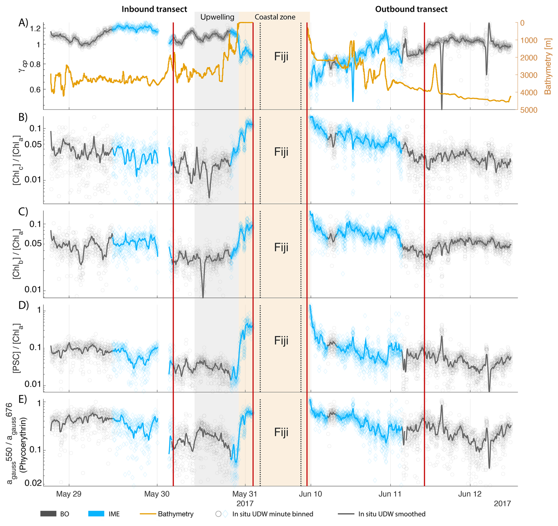
Figure 7 Underway bio-optical proxies for changes in community composition measured during the inbound (left panels) and outbound (right panels) transects around Fiji. (A) mean particle size index (${\mathit{\gamma }}_{c_{\mathrm{p}}}$), (B) Chlorophyll c normalized by [Chl a] ($\left[\mathrm{Chl}c\right]/\left[\mathrm{Chl}a\right]$; indicative of diatoms and other red algae), (C) Chlorophyll b normalized by [Chl a] ($\left[\mathrm{Chl}b\right]/\left[\mathrm{Chl}a\right]$; indicative of green algae), (D) photosynthetic carotenoids normalized by [Chl a] ($\left[\mathrm{PSC}\right]/\left[\mathrm{Chl}a\right]$; indicative of diatoms), and (E) Phycoerythrin particulate gaussian absorption at 550 nm normalized by [Chl a] particulate gaussian absorption at 676 nm ($a_{\mathrm{gauss}}\mathrm{550}/a_{\mathrm{gauss}}\mathrm{676}$; indicative of cyanobacteria). The blue points show in situ data falling in IME zones detected on the overlapping 8 d satellite composite (BO = black circle, IME = blue diamond). The points show the minute-binned underway data, and the solid lines represent the underway data smoothed with a 2 h low-pass digital filter. The gray shaded area highlights the coastal upwelling zone, and the beige shaded area highlights the transect over shallow waters (<100 m depth). The red vertical lines represent the start and end times of the inbound and outbound transect sections shown in Fig. 6.

3.4 Temporal dynamics

The IME detected around Fiji-Tonga, increased in surface and surface-area integrated [Chl a] from the end of February to early May 2017, when it covered more than one million square kilometers. The impacted area then decreased between May and the end of August 2017 (Fig. 8B). The difference in Φ_Sat between the IME and the BO (ΔΦ_Sat) was consistently negative, indicating a lower phytoplankton physiological stress and a net enrichment in iron in the Fiji-Tonga IME relative to the BO, especially at the beginning of the time-series, during the expanding phase of the IME (i.e. February to May). Φ_Sat in the IME decreased overall during the studied period, suggesting an increase in iron enrichment in the IME. The difference in ϕ_sat between the IME and BO (i.e. ΔΦ_sat) remained statistically significant ($\left|\mathrm{\Delta }{\mathrm{\Phi }}_{\mathrm{sat}}\right|>{\text{SEM}}_{\mathrm{\Delta }{\mathrm{\Phi }}_{\mathrm{sat}}}^{\mathrm{f}}$), indicating persistent iron enrichment within the IME associated with Fiji-Tonga. However, $\left|\mathrm{\Delta }{\mathrm{\Phi }}_{\mathrm{sat}}\right|$ decreased over the six-month period, approaching but not reaching zero, implying that Φ_Sat values in the IME became more similar to those in the BO. Because Φ_Sat within the IME also decreased over this period, this trend suggests that Φ_Sat decreased more strongly in the BO than in the IME. This pattern is consistent with an increase in iron availability in the BO, which reduced the contrast in Φ_Sat between the IME and BO. These results indicate the presence of seasonal variability in iron stress within the BO and suggest that the processes controlling this variability differ from those governing iron enrichment within the IME. Phytoplankton communities in the IME were not experiencing stress due to macronutrient limitation during the expanding phase of the IME (i.e. February to May with ${\mathit{\eta }}^{\prime }<\mathrm{0.2}$) but started to experience a moderate stress three weeks before the end of the expansion phase of the bloom (i.e. $\mathrm{0.2}<{\mathit{\eta }}^{\prime }\le \mathrm{0.6}$). Φ_Sat and η^′ were significantly lower in Fiji-Tonga's IME relative to the BO, even during bloom demise, suggesting that top-down controls, such as grazing, contributed to the bloom demise before the iron and macronutrients were fully depleted from the euphotic zone in the IME.

Samoa's IME was characterized by two important phytoplankton biomass accumulation phases (i.e. blooms) over the period studied, highlighted by two distinct IME-surface-area integrated [Chl a] peaks around 9 November and 19 December 2016 (Fig. E3). Interestingly, in Samoa's IME, iron and macronutrient stress did not decrease before and during the initiation of the first of these two blooms and were consistently lower in the IME compared to the BO along the entire time series, which suggests that the occurrence of the first bloom in Samoa's IME was not only triggered by bottom-up processes such as macronutrient and iron enrichment. This first bloom only initiated after being advected offshore and detached from the coastal IME of Samoa, which coincided with the dilution of coastal waters into the BO. This dilution may have decreased the encounter rate between grazers and their prey, reducing the grazing pressure, while the high levels of macronutrients and iron advected within this water mass maintained phytoplankton growth rate, allowing for positive accumulation of phytoplankton biomass (such as hypothesized in Lehahn et al., 2017; Bourdin et al., 2025). This hypothesis is also supported by the similarities in physical properties of Samoa's advected IME and the ones of its coastal IME (i.e. warmer and fresher than the BO south of Samoa; Figs. B6 and B7), which suggest that the water mass advected offshore had a coastal origin (see Sect. 3.1 and Appendix B).

While these results suggest continuous enrichments in iron and macronutrients in IME zones in the western South Pacific Ocean, the results are more contrasted in the eastern South Pacific Ocean where Φ_Sat and η^′ in IME areas are often not significantly lower than in the BO (illustrated by $\mathrm{\Delta }{\mathrm{\Phi }}_{\mathrm{Sat}}+{\text{SEM}}_{\mathrm{\Delta }{\mathrm{\Phi }}_{\mathrm{Sat}}}^{\mathrm{f}}>\mathrm{0}$ or $\mathrm{\Delta }{\mathit{\eta }}^{\prime }+{\text{SEM}}_{\mathrm{\Delta }{\mathit{\eta }}^{\prime }}^{\mathrm{f}}>\mathrm{0}$; Appendix E, Figs. E1 and E2).

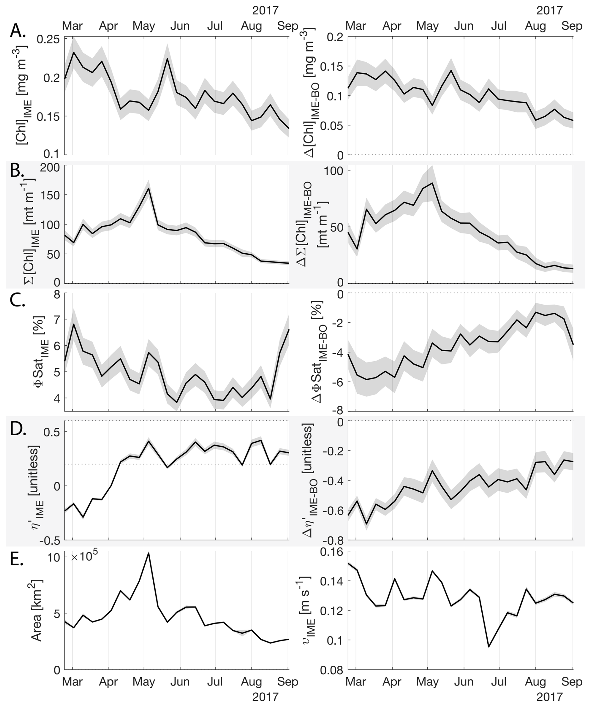
Figure 8 Six-month-long time series of satellite-derived IME properties of the IME zone detected around Fiji and Tonga archipelagos combined. (A), (B), (C), and (D) left panels: Average of properties within the IME zones, (A), (B), (C), and (D) right panels: Difference between properties within the IME zones and the background ocean (BO). (A) row: chlorophyll a concentration ([Chl a]), (B) row: IME integrated [Chl a] (∑[Chl a]_IME), (C) row: fluorescence quantum yield (ϕ_Sat; iron stress index), (D) row: macronutrient stress index (η^′), (E) left: IME zone area (in km²), (E) right: surface current velocity. The shaded areas represent the standard errors propagated following the method in Appendix A4.

3.5 Relating IME properties to characteristics of islands

Although the four cases studied were sampled during different seasons, we detected a longitudinal gradient in the strength of the IME and its associated iron enrichment (i.e. from Rapa Nui to Fiji) in the SPSG. However, this longitudinal gradient should be interpreted with caution, as the size of the IME area is correlated with the size of islands (Fig. 9A), highlighting that island size can be an important driver of IME magnitude.

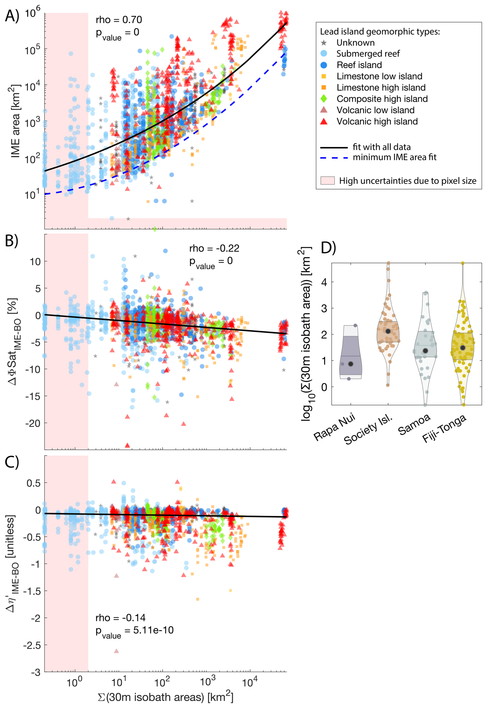
Figure 9 Relationship between the summed 30 m isobath areas of all islands and reefs associated with each individual IME and the IME area (A), the difference between average fluorescence quantum yield (ϕ_Sat; iron stress index) in IME and BO (B), the difference between average macronutrient stress index (η^′) in IME and BO (C). The black solid line represents a robust second-order polynomial fit (A) and linear fits (B, C). The blue dashed line represents the second-order polynomial fit of the minimum IME area prediction (A). Different colors and marker shapes represent the different island/reef geomorphic types from the Nunn et al. (2016) island database. The shaded polygons represent high uncertainty areas due to pixel size. Subplot (D) represents the distributions of 30 m isobath areas of all islands contributing to IMEs in each region.

The Σ(30 m isobath area) effectively predicts the potential minimum IME area using a second-order polynomial model (dashed blue line in Fig. 9A):

$$\begin{array}{}\text{(7)}& {\log }_{\mathrm{10}}\left({\mathrm{IME}}_{{\mathrm{area}}_{\min \mathrm{predicted}}}\right)=\mathrm{1.114}+\mathrm{0.281}X+\mathrm{0.105}{X}^{\mathrm{2}}\end{array}$$

where X=log ₁₀(Σ(30 m isobath area)). However, it is insufficient to accurately predict the mean strength and spatial extent of the IME, as evidenced by the large variability in IME area observed for a given Σ(30 m isobath area) (Fig. 9A).

Other factors associated with nutrient supply mechanisms that are independent of island size – such as the stoichiometry of macronutrients and trace metals arising from different sources, phytoplankton community composition, and grazing pressure – also play an important role in determining the magnitude of the IME.

The rank in the magnitude of the IME observed in Figs. 4 and B1 (Fiji-Tonga > Samoa > Society Islands > Rapa Nui) does not correspond to the rank of the island/reef area contributing to the IME of each region (Fig. 9D). For example, the total 30 m isobath areas of all islands and reefs that contributed to the IMEs in the Society Island region are larger on average than the total 30 m isobath areas of Samoa and Fiji-Tonga (Fig. 9D). Island/reef size is represented here as the sum of all 30 m isobaths associated with an IME, which in the case of the Society Islands region, encompasses the Society Islands themselves, but also the Tuamotu archipelago, which is composed of 76 islands and atolls, some of which are among the largest atolls on the planet (e.g. Rangiroa covering 1640 km²). Their land area relative to their 30 m isobath area is very small, therefore, the terrigenous inputs of these coral reef atolls are likely smaller in comparison to those of the large high islands of Viti Levu and Vanua Levu of Fiji's archipelago. Moreover, islands of different geomorphic types may have different stoichiometries of macronutrient and iron enrichment. For example, volcanic islands are known to be sources of iron in the water column (Bonnet et al., 2023; Guieu et al., 2018), thus their IMEs may have, on average, higher $\mathrm{\Delta }{\mathrm{\Phi }}_{{\mathrm{Sat}}_{\mathrm{IME}-\mathrm{BO}}}$ than the IMEs located around coral atolls. Our results, however, do not show clear trends between the geomorphic types of islands and their associated IME area or nutrient stress (Fig. 9). The lack of a clear trend may result from the multiple sources of variability inherent to this study (e.g., seasonal variability, regional variability in oceanographic conditions, variability in responses of different phytoplankton assemblages to macronutrient and iron enrichment), which could mask the signal. Although characterized by weak correlations, the iron and nutrient enrichments associated with IMEs increased with larger reef/islands, which is illustrated here by the negative correlation between Σ(30 m isobath area) and $\mathrm{\Delta }{\mathrm{\Phi }}_{{\mathrm{Sat}}_{\mathrm{IME}-\mathrm{BO}}}$ and $\mathrm{\Delta }{\mathit{\eta }}_{\mathrm{IME}-\mathrm{BO}}^{\prime }$.

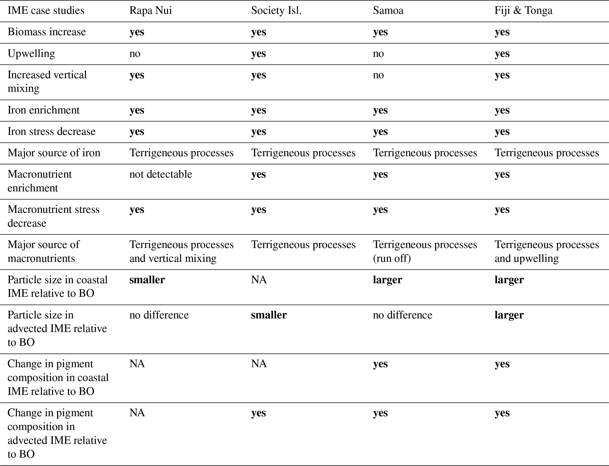
Table 3 Summary results of IME characteristics of Rapa Nui, Society islands, Samoa, and Fiji-Tonga archipelagos. Refer to Fig. B1 for quantitative interpretation. The bold font highlights the significant differences between IME and BO.

NA: not available.

4 Conclusions

In this study, we used a combination of satellite-derived physiological stress markers and in situ optical data from an underway system to elucidate the links between IME, phytoplankton physiology, and pigment ratios as proxies for community composition on the scale of the subtropical basin of the South Pacific. To our knowledge, such an endeavor has never been done.

Each of the four case studies exhibited unique spatial and temporal dynamics of IME (see result summary Table 3), yet in all cases we observed indications of a relaxation of iron stress in the IME relative to the regional surrounding ocean. Our results support the idea that islands or reefs also contribute to macronutrient enrichment from terrigenous origins, but unlike total iron concentrations, which generally remain higher over entire IME zones, macronutrients are typically rapidly depleted by the time a given coastal water mass is advected into the open ocean. This rapid depletion is associated with pigments ratio signatures indicating higher proportions of diatoms near shore, which outcompete other phytoplankton for nitrate uptake (Litchman et al., 2007; Smith et al., 2019). This interpretation, however, remains hypothetical and requires further verification using quantitative imaging or genomic tools to study plankton community composition. The offshore IME water masses were associated with macronutrient enrichment originating from upwelling and vertical mixing processes in the western basin of the SPSG. Although detected in the eastern SPSG, these upwelling and vertical mixing signatures (i.e. low-light-adapted phytoplankton cells around islands) were not necessarily associated with significant macronutrient enrichment in the eastern SPSG, possibly due to the nutricline being deeper than in the western basin. The island and reef isobath area is a strong predictor of the minimum IME area and a weaker predictor of the associated macronutrient and iron enrichment. However, the high spatial and temporal variability of IME extent across the SPSG suggests that its magnitude is strongly influenced by complex interactions among initial phytoplankton stocks, bottom-up processes (i.e. stoichiometry of macronutrient and trace metal supply), and top-down controls (i.e. grazing pressure).

Building on these findings and previous IME-focused studies of natural iron enrichment (e.g. Galápagos PlumeEx and Kerguelen KEOPS; Coale et al., 1998; Blain et al., 2008), we propose that IMEs constitute naturally persistent nutrient enrichment settings that can be further exploited to investigate the combined effects of iron and macronutrient supply on natural plankton assemblages, net primary production, and carbon export at basin scales. However, the uniqueness of each combination of factors that influence IMEs requires case-by-case studies, including temporal dynamics, to reveal specific underlying processes. In this context, the use of satellite data to detect upwellings, macronutrients, and iron enrichment to survey entire ocean basins is promising, especially with the recent deployment of the hyperspectral mission Plankton, Aerosol, Cloud, and Ocean Ecosystem (PACE) that can provide crucial information on phytoplankton community composition necessary to complement the interpretation of physiological signals. There is also a need to further validate these satellite-based estimates of iron and macronutrient stress, such as molecular markers from metatranscriptomic analyses, to enhance our confidence in the macronutrient and iron enrichment patterns deduced from remote sensing products and identify taxa-specific physiological responses.

Appendix A: Satellite variable computation

Figure A1 Satellite composite production flowchart.

A1 Satellite intermediate products computation

We derived the normalize leaving water radiance spectra (nL_w) from POLYMER normalized water reflectance spectra (R_w):

$$\begin{array}{}\text{(A1)}& \mathrm{n}{L}_{\mathrm{w}}\left(\mathit{\lambda }\right)=R_{\mathrm{w}}\left(\mathit{\lambda }\right)\times {\displaystyle \frac{F_{\mathrm{0}}}{\mathit{\pi }}}\end{array}$$

where F₀ is the extraterrestrial solar flux at the time of observation:

$$\begin{array}{}\text{(A2)}& F_{\mathrm{0}}=F_{{\mathrm{0}}_{\mathrm{mean}}}\left(\mathit{\lambda }\right)\times {\left({\displaystyle \frac{d}{d_{\mathrm{mean}}}}\right)}^{\mathrm{2}}\end{array}$$

where $F_{{\mathrm{0}}_{\mathrm{mean}}}\left(\mathit{\lambda }\right)$ is the solar spectral irradiance in  $\mathrm{W}{\mathrm{m}}^{-\mathrm{2}}\mathrm{\mu }{\mathrm{m}}^{-\mathrm{1}}$ based on Thuillier et al. (2003) and spectrally weighted to each sensor's band spectral response, and where ${\left(\frac{d}{d_{\mathrm{mean}}}\right)}^{\mathrm{2}}$ is the normalized Sun-Earth distance at the time of observation (Whiteman and Allwine, 1986).

The normalized fluorescence line height (nFLH) was calculated from nL_w as in Behrenfeld et al. (2009):

$$\begin{array}{}\text{(A3)}& \begin{array}{rl}\text{nFLH}& =\mathrm{n}{L}_{\mathrm{w}}\left(\mathrm{678}\right)\mathrm{-}\left({\displaystyle \frac{\mathrm{70}}{\mathrm{81}}}\right)\times \mathrm{n}{L}_{\mathrm{w}}\left(\mathrm{667}\right)\\ & \mathrm{-}\left({\displaystyle \frac{\mathrm{11}}{\mathrm{81}}}\right)\times \mathrm{n}{L}_{\mathrm{w}}\left(\mathrm{748}\right)\end{array}\end{array}$$

We estimated SST from MODIS-Aqua and Terra, and VIIRS-SNPP L1A scenes using SeaDAS l2gen and only keeping high-quality pixels (i.e. 0 and 1 SST quality scores).

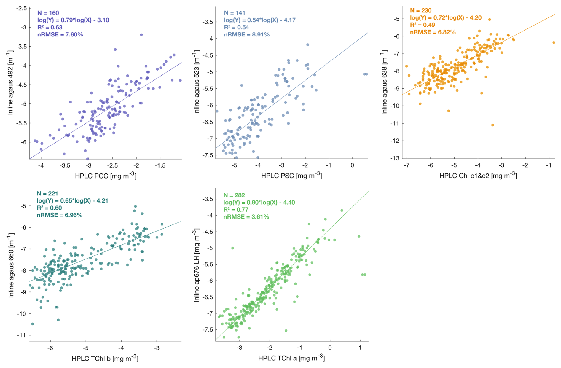
Figure A2 Robust linear regressions between phytoplankton pigments measured from HPLC and optical proxies for phytoplankton pigments estimated from a_p spectra (Chase et al., 2013) from the underway system (in log $/$ log scale) during the Tara Pacific expedition (May 2016 to October 2018).

A2 in situ to satellite Match-ups

Match-ups between the calibrated in situ data collected from the underway system and level-2 satellite data of each satellite processed were performed following recommendations from Bailey and Werdell (2006). Underway data falling within ±3 h of each satellite overpass were extracted and averaged. We extracted and averaged underway measurements within a ±3 h period of each satellite overpass (i.e. Aqua and SNPP 13:30, Terra 10:30, Sentinel 3a and 3b 10:00, JPSS1 14:20 local time at the equator) and satellite data from the 25 closest pixels to underway data locations. We computed the median coefficient of variation (CV) of nL_w for bands between 412 and 555 nm and for the aerosol optical thickness at 865 nm. We tested several homogeneity thresholds and minimum unmasked number of pixels for each parameter matched to maximize the number of valid match-ups without introducing noise to the in situ-satellite correlations. We kept only [Chl a] match-ups with a minimum of 7 unmasked pixels and CV lower than 0.15 (Fig. A3c and see Appendix B in Bourdin et al., 2025). We kept iPAR match-ups with a minimum of 5 unmasked pixels and CV lower than 0.7 (Fig. A3b). The SST quality score being already very restrictive, we kept match-ups with at least one unmasked pixel (i.e. SST-quality 0 and 1; Fig. A3a). The statistics of these match-up relations were subsequently used to select the atmospheric correction and [Chl a] algorithm performing best in our case (Brewin et al., 2015) and the normalized root mean square errors (nRMSE) were used as uncertainty estimates and were propagated to subsequent products (see comparison in Appendix B in Bourdin et al., 2025, and uncertainty propagation in Appendix A4 of this study).

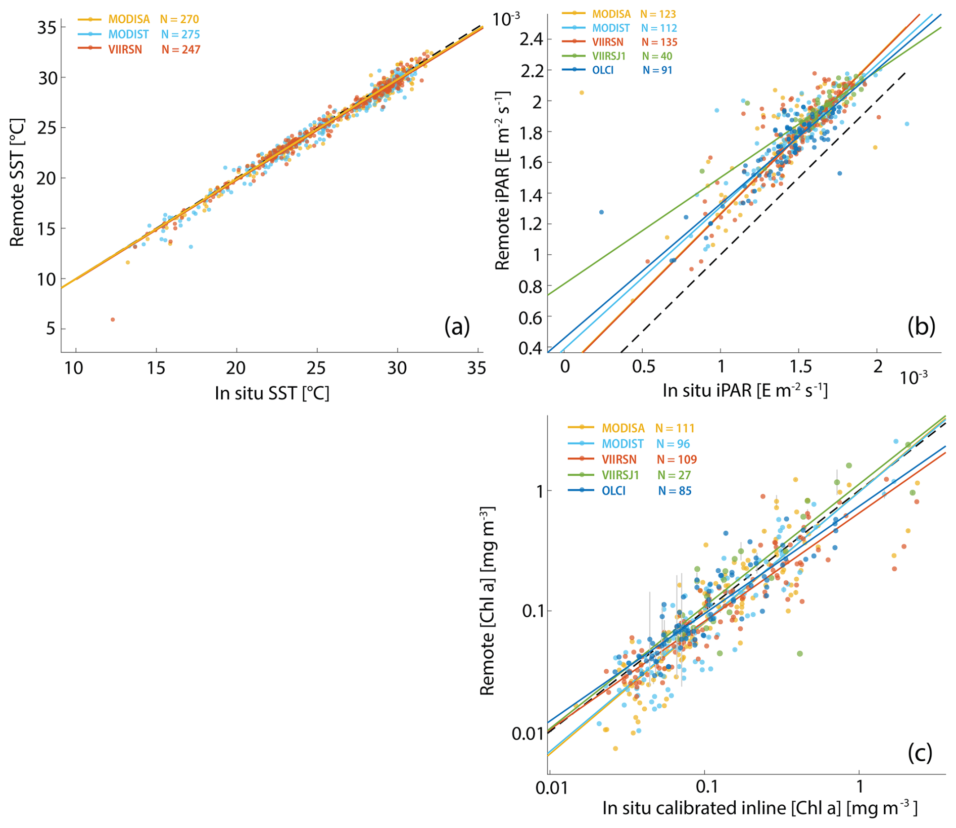
Figure A3 Robust linear regressions between in situ and satellite SST (a), iPAR (b), and [Chl a] (c) computed with the blended OCx-CI algorithm and POLYMER R_rs. The in situ data were measured during the Tara Pacific expedition (May 2016 to October 2018).

Table A1 Robust correlations parameters of match-ups between satellite and in situ underway data

A3 MODIS b_bp artifacts

b_bp estimated from MODIS POLYMER R_rs (Fig. A4.2a and b) showed inverse spatial patterns compared to [Chl a] computed from all sensors (Fig. A4.3) and also b_bp estimated from OLCI and VIIRSN R_rs (Fig. A4.2c and d) in ultra-oligotrophic regions ([Chl a]<0.04 mg m⁻³). These inverse spatial patterns were not observed with b_bp computed from SeaDAS R_rs (Fig. A4.1a, b, c, and d). The atmospheric correction of SeaDAS (i.e. l2gen) does not correct for the adjacency effect, while POLYMER does (i.e. the last term of the polynomial fit used to model the atmospheric reflectance accounts for the adjacency effect). The b_bp values in ultra-oligotrophic regions were largely within the range of noise added by the adjacency effect around clouds. Subsequently, the 8 d median b_bp products computed from SeaDAS R_rs for each satellite were so noisy that most of the signal due to the b_bp artifact in ultra-oligotrophic regions was masked by the adjacency effect. Therefore, only b_bp from VIIRSN and OLCI were binned into the 8 d median and used in further analysis.

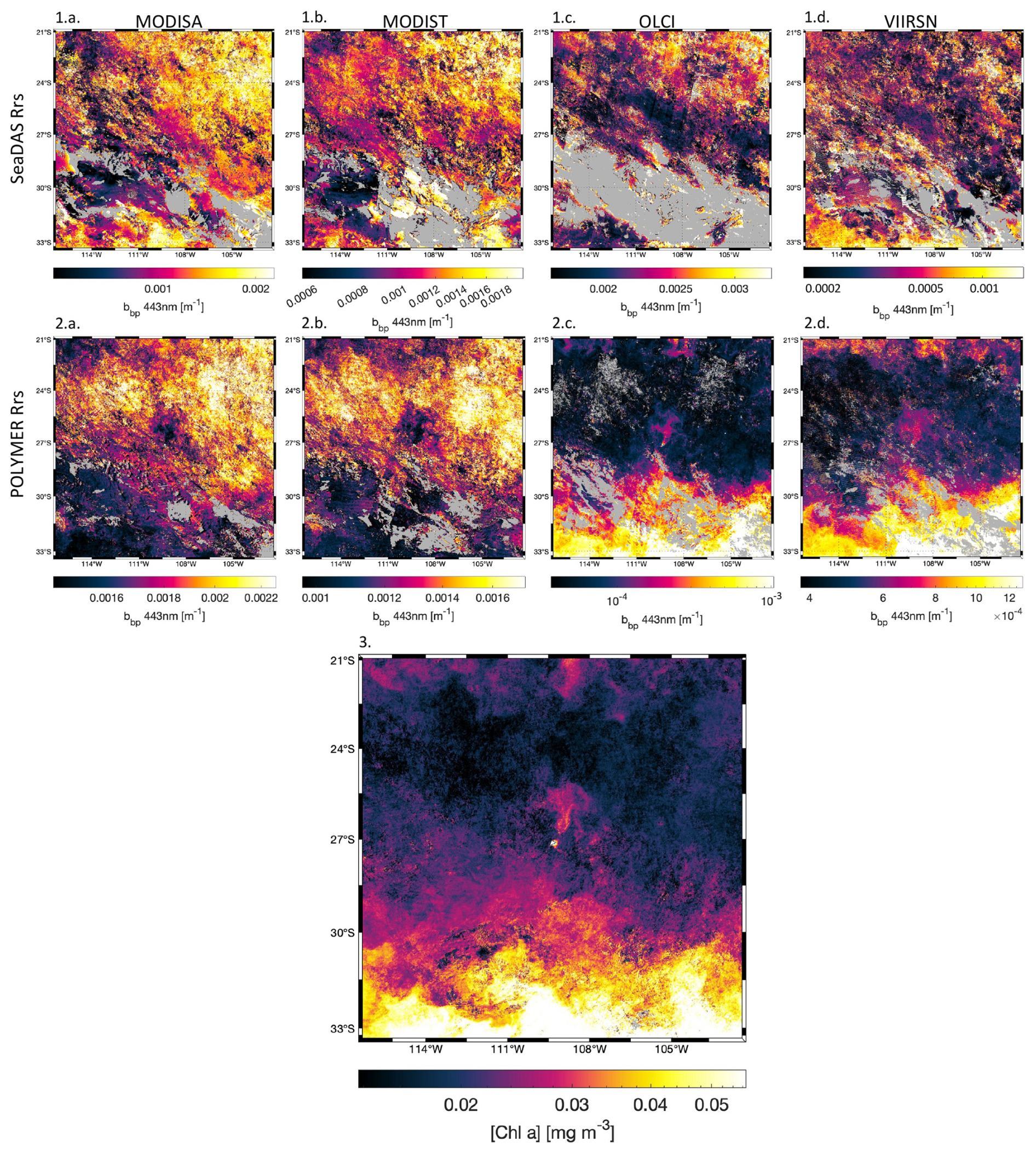
Figure A4 Comparison of 8 d medians (11 to 18 October 2016) of b_bp around Rapa Nui for (a) MODISA, (b) MODIST, (c) OLCI, and (d) VIIRSN, using the atmospheric corrections (1) SeaDAS R_rs (top row), (2) POLYMER R_rs (middle row), and (3) the corresponding 8 d median of [Chl a] computed using POLYMER R_rs of all satellites.

A4 Uncertainty estimates

The 8 d merged satellite product composites were derived as described for [Chl] in Bourdin et al. (2025), using multiple overpasses and sensors. For the 2500 km² region around the Fiji archipelago, composites typically include ∼120 daytime ocean color scenes and ∼240 SST scenes (daytime and nighttime). Each pixel of the merged products is a median of the n number of observations of the original images, with standard deviations (σ_bin) representing the temporal variability for a given pixel during each 8 d period and the variability between sensors (after nudging, when applied). We computed Φ_Sat only from the MODIS and OLCI sensors due to a missing band in VIIRS for the computation of nFLH. Binned b_bp were only obtained from OLCI and VIIRS sensors due to an artifact in the MODIS estimates of this variable (Appendix A3). Therefore, the number of observations in the binned Φ_Sat and b_bp was reduced, resulting in noisier maps.

We propagated known uncertainties from in situ data to satellite merged end-products following the same strategy as in Bourdin et al. (2025). We estimated the error associated with the computation of bio-optical proxies from in situ continuous underway data, using the normalized root mean square error (nRMSE_udw in %) of the correlation between the underway estimates and their corresponding calibrated measurement when available (e.g. total [Chl a] from HPLC correlated with [Chl a] line-height in Bourdin et al. (2025)). Similarly, we estimated the error associated with bio-optical proxies computation from satellite data using the nRMSE_sat of the relation between each satellite estimate and its calibrated underway counterpart when available (e.g. [Chl a] see Appendix B in Bourdin et al., 2025, and SST and iPAR in Fig. A3 and Table A1). Since no measurements of C_phyto were performed in situ, we propagated to the binned C_phyto the uncertainty estimates of the published empirical relationships we used between b_bp and C_phyto (32 %; Graff et al., 2015)). Unfortunately, the relation between in situ b_bp and satellite b_bp was very sensitive to match-up criteria and the linear regressions were not well constrained, potentially due to low quality of in situ data (due to bio-fouling or bubbles in the underway line) or due to large uncertainty in satellite retrieval (Bisson et al., 2021). Therefore, b_bp, like all the other variables for which no calibrated in situ data were available, was nudged to best match a reference satellite sensor (see Sect. 2.5). In these cases, the error associated with the nudging process (i.e. nRMSE_sat of the regressions) was propagated to the binned products' uncertainty estimates. In all of these cases, the uncertainties of the binned satellite end-products were computed as follows:

$$\begin{array}{}\text{(A4)}& {\mathit{\sigma }}_V=\sqrt{{\mathit{\sigma }}_{V\mathrm{bin}}^{\mathrm{2}}+\sum _{n=\mathrm{1}}^{n_{\mathrm{c}}}(\stackrel{\mathrm{̃}}{V}\cdot {\text{nRMSE}}_{\mathrm{c}}{)}^{\mathrm{2}}}\end{array}$$

with $\stackrel{\mathrm{̃}}{V}$ the binned variable, n_c the number of calibration/correction, and nRMSE_c the nRMSE associated with each of the n_c corrections. The uncertainty associated with the correction of each variable was saved in the data files (Bourdin, 2025). When no good relationship with in situ data or reference satellite data was found, “NaN” values are saved in the nRMSE columns of the data files. In these cases, the final σ_V of a given 8 d median pixel only represents the natural variability over the 8 d period and the variability between sensors. The standard error of the mean of the adjusted satellite end-products of each pixel was computed as follows:

$$\begin{array}{}\text{(A5)}& {\mathrm{SEM}}_V={\displaystyle \frac{{\mathit{\sigma }}_V}{\sqrt{n_{V_{\mathrm{bin}}}}}}\end{array}$$

The final uncertainty estimate associated with the adjusted satellite binned variable (V) within the entire IME or BO zones (${{\mathrm{SEM}}^{\mathrm{f}}}_{[V{]}_{\mathrm{IME}}}$) as presented in Figs. E1, E2, E3, and 8 were expressed as the mean standard error of the mean of V within entire IME or BO zones:

$$\begin{array}{}\text{(A6)}& {{\mathrm{SEM}}^{\mathrm{f}}}_{V_{\mathrm{IME}}}={\displaystyle \frac{{\stackrel{\mathrm{‾}}{\mathit{\sigma }}}_{V_{\mathrm{IME}}}}{\sum n_{V_{{\mathrm{bin}}_{\mathrm{IME}}}}}}+S_{V_{\mathrm{unc}}}\times {\stackrel{\mathrm{‾}}{V}}_{\mathrm{IME}}\end{array}$$

with $\sum n_{V_{{\mathrm{bin}}_{\mathrm{IME}}}}$ the total number of V observations within the IME zone before merging, and $S_{V_{\mathrm{unc}}}$ the weighted bias associated with the calculation of the slopes of the regressions between the calibrated in situ variable and each satellite estimate V. $S_{V_{\mathrm{unc}}}$ was computed as follows:

$$\begin{array}{}\text{(A7)}& S_{V_{\mathrm{unc}}}=|\mathrm{1}-S_{V_{\mathrm{sat}}}|\times {\displaystyle \frac{n_{M_{\mathrm{sat}}}}{N_{M_{\mathrm{tot}}}}}\end{array}$$

with $S_{V_{\mathrm{sat}}}$ the slope of the relation between V of a given satellite and its in situ equivalent, $n_{M_{\mathrm{sat}}}$ the number of valid match-ups of the same satellite, and $N_{M_{\mathrm{tot}}}$ the total number of valid match-ups. $S_{V_{\mathrm{unc}}}$ represents the maximum bias associated with the calculation of the merged satellite variable V, which we assume to be equivalent to the potential likelihood bias of the merged satellite variable V. Assuming sufficient valid matches with each satellite, $S_{V_{\mathrm{unc}}}$ is a conservative estimate of the bias associated with the slope computation because the merging method forces each satellite V to agree with in situ data using sensor-specific corrections, which likely reduces the bias of the merged product. This method was applied to compute the uncertainty of all satellite merged variables except η^′, the IME surface area, and the surface-area integrated [Chl a] (∑[Chl a]_IME). IME area uncertainties (${\mathit{\sigma }}_{A_{\mathrm{IME}}}$) were computed during the detection of the IME [Chl a] contours as the difference in the IME area between the last two iterations of the [Chl a] contours:

$$\begin{array}{}\text{(A8)}& {\mathit{\sigma }}_{A_{\mathrm{IME}}}=A_{{\mathrm{IME}}_{{\mathrm{cChl}}_f}}-A_{{\mathrm{IME}}_{{\mathrm{cChl}}_{f-\mathrm{1}}}}\end{array}$$

with $A_{{\mathrm{IME}}_{{\mathrm{cChl}}_f}}$ the IME area at the final IME contour value and $A_{{\mathrm{IME}}_{{\mathrm{cChl}}_{f-\mathrm{1}}}}$ the IME area at the previous contour value. Therefore, ${\mathit{\sigma }}_{A_{\mathrm{IME}}}$ represents the area detection resolution associated with the size of the step of [Chl a] iteration. The uncertainties associated with the estimation of IME surface-area integrated [Chl a] (∑[Chl a]_IME) were computed as follows:

$$\begin{array}{}\text{(A9)}& \begin{array}{rl}{{\mathrm{SEM}}^{\mathrm{f}}}_{\sum [\mathrm{Chl}a{]}_{\mathrm{IME}}}& =\sum [\mathrm{Chl}a{]}_{\mathrm{IME}}\\ & \times \sqrt{{\left({\displaystyle \frac{{{\mathrm{SEM}}^{\mathrm{f}}}_{[\mathrm{Chl}a{]}_{\mathrm{IME}}}}{{\stackrel{\mathrm{‾}}{\left[\mathrm{Chl}a\right]}}_{\mathrm{IME}}}}\right)}^{\mathrm{2}}+{\left({\displaystyle \frac{{\mathit{\sigma }}_{A_{\mathrm{IME}}}}{A_{\mathrm{IME}}}}\right)}^{\mathrm{2}}}\end{array}\end{array}$$

We estimated uncertainties in ${\mathit{\eta }}_{\mathrm{obs}}^{\prime }$ (i.e. $\left[\mathrm{Chl}a\right]/\left[C_{\mathrm{phyto}}\right]$) as:

$$\begin{array}{}\text{(A10)}& {\mathrm{SEM}}_{{\mathit{\eta }}_{\mathrm{obs}}^{\prime }}={\mathit{\eta }}_{\mathrm{obs}}^{\prime }\times \sqrt{{\left({\displaystyle \frac{{\mathrm{SEM}}_{\left[\mathrm{Chl}a\right]}}{\left[\mathrm{Chl}a\right]}}\right)}^{\mathrm{2}}+{\left({\displaystyle \frac{{\mathrm{SEM}}_{\left[C_{\mathrm{phyto}}\right]}}{\left[C_{\mathrm{phyto}}\right]}}\right)}^{\mathrm{2}}}\end{array}$$

Similarly:

$$\begin{array}{}\text{(A11)}& {\mathrm{SEM}}_{I_{\mathrm{ML}}}=I_{\mathrm{ML}}\times \sqrt{{\left({\displaystyle \frac{{\mathrm{SEM}}_{\mathrm{PAR}}}{\mathrm{PAR}}}\right)}^{\mathrm{2}}+{\left({\displaystyle \frac{{\mathrm{SEM}}_{\mathrm{MLD}}}{\mathrm{MLD}}}\right)}^{\mathrm{2}}+{\left({\displaystyle \frac{{\mathrm{SEM}}_{{\mathrm{Kd}}_{\mathrm{PAR}}}}{{\mathrm{Kd}}_{\mathrm{PAR}}}}\right)}^{\mathrm{2}}}\end{array}$$

where SEM_PAR is the standard error of the mean of the merged daily PAR product, ${\mathrm{SEM}}_{\mathrm{MLD}}=max(\mathrm{0.2}\times \mathrm{MLD}$, 5 m), and ${\mathrm{SEM}}_{{\mathrm{Kd}}_{\mathrm{PAR}}}={\mathrm{SEM}}_{\left[\mathrm{Chl}a\right]}$ since Kd_PAR is estimated from the [Chl a] merged products.

Since η^′ ranges from negative to positive values, we expressed its uncertainties as follows:

$$\begin{array}{}\text{(A12)}& {\mathrm{SEM}}_{{\mathit{\eta }}^{\prime }}=\left|{\mathit{\eta }}^{\prime }\right|\times \sqrt{{\left({\displaystyle \frac{{\mathrm{SEM}}_{I_{\mathrm{ML}}}}{I_{\mathrm{ML}}}}\right)}^{\mathrm{2}}+{\left({\displaystyle \frac{{\mathrm{SEM}}_{{\mathit{\eta }}_{\mathrm{obs}}^{\prime }}}{{\mathit{\eta }}_{\mathrm{obs}}^{\prime }}}\right)}^{\mathrm{2}}}\end{array}$$

We assumed that the uncertainties associated with the computation of ${\widehat{\mathit{\eta }}}_{{\mathrm{obs}}_{\min }}$ and ${\widehat{\mathit{\eta }}}_{{\mathrm{obs}}_{\max }}$ fits were negligible compared to ${\mathrm{SEM}}_{I_{\mathrm{ML}}}$ and ${\mathrm{SEM}}_{{\mathit{\eta }}_{\mathrm{obs}}^{\prime }}$, given the substantial number of valid ${\mathit{\eta }}_{\mathrm{obs}}^{\prime }$ pixels per I_ML bin used to compute ${\widehat{\mathit{\eta }}}_{{\mathrm{obs}}_{\min }}$ and ${\widehat{\mathit{\eta }}}_{{\mathrm{obs}}_{\max }}$ fits (on average 1.13×10⁷ pixels per I_ML bin). Since the mixed layer is often shallower than Z_eu in this region, ${\mathrm{Kd}}_{{\mathrm{PAR}}_{Z_{\mathrm{eu}}}}>{\mathrm{Kd}}_{{\mathrm{PAR}}_{\mathrm{MLD}}}$. Therefore, we tested the sensitivity of η^′ computation using two different empirical methods to estimate Kd_PAR from [Chl a]. In addition to the method presented in Sect. 2.4 for computing Kd_PAR from Z_eu, we estimate Kd₄₉₀ from [Chl a] and Kd_PAR from Kd₄₉₀ using Eqs. (8) and (9) from Morel et al. (2007). Differences in η^′ were negligible in all four case studies (that is, the maximum difference ranging from 10⁻³ to 0.05), and the spatial and temporal trends remained consistent between the two calculation methods.

Appendix B: Phytoplankton physiology in Rapa Nui, Society Islands, Samoa, and Fiji-Tonga' IMEs

We aggregated satellite data from all IME and BO pixels of each studied archipelago across the 6-month time series to quantify differences between IME and BO regions and compare these differences among archipelagos. We assessed normality independently for each category using a Lilliefors test. When all categories satisfied the normality assumption, differences were evaluated using a parametric analysis of variance (ANOVA); otherwise, a non-parametric Kruskal–Wallis test was applied. Because each violin plot represents a very large number of observations (i.e. between 2.5 and 12 million data points), statistically significant differences were detected for all variables between IME and BO regions; however, the magnitude of these differences varies among parameters and regions and should be interpreted accordingly.

We analyzed inbound and outbound transects around Rapa Nui, Society Islands, and Samoa to identify processes associated with potential nutrient enrichments, as done in Sect. 3.2 for Fiji. In these three case studies, b_bp was not measured in situ, therefore, we computed the ratio between [Chl a] and c_p660 ($\left[\mathrm{Chl}a\right]/c_{\mathrm{p}}\mathrm{660}$) as an alternative for $\left[\mathrm{Chl}a\right]/\left[C_{\mathrm{phyto}}\right]$ (Figs. B2, B4, B6; Behrenfeld and Boss, 2006). These results show that $\left[\mathrm{Chl}a\right]/c_{\mathrm{p}}\mathrm{660}$, measured in situ along the transects, generally follows similar spatial trends to $\left[\mathrm{Chl}a\right]/\left[C_{\mathrm{phyto}}\right]$ measured from satellite data, although the magnitude of these two ratios differs significantly. In all three cases, sudden synchronized changes in SST and SSS were detected along the inbound and outbound transects, indicating the presence of fronts between different water masses. These water mass changes were accompanied by higher $\left[\mathrm{Chl}a\right]/c_{\mathrm{p}}\mathrm{660}$ in the IME zone on the outbound transects of Rapa Nui (Fig. B2) and the Society Islands (also associated with lower $\left[\mathrm{PPC}\right]/\left[\mathrm{Chl}a\right]$ in that case; Fig. B4), suggesting the upwelling of low-light-adapted cells to the surface. No evidence of such upwelling was detected around Samoa; however, the strong increase in SST and decrease in SSS detected while crossing the IME zone south of Samoa on the inbound transect indicate a front between BO waters and IME waters. The IME zone properties were similar to those of coastal water masses characterized by significantly high nitrogen concentrations for the region (up to 1 µM of dissolved organic nitrogen), higher SST, and lower, more variable SSS, which are typical of water masses influenced by freshwater discharge (Fig. B6). These findings suggest that the IME zone observed offshore along the inbound transect was likely caused by nitrogen inputs from terrigenous sources, discharged into the coastal ocean via rivers, and subsequently advected offshore by coastal currents. Figure B5 reveals an artificially sharp line of increasing Φ_Sat across the outbound transect, likely due to an anomaly in nFLH or iPAR estimation. To avoid misinterpretation, this section was removed from Fig. B4 on the outbound transect. Overall, Φ_Sat consistently decreased when approaching each of these three islands, and was generally associated with increased total iron concentration, although two stations exhibited low total iron concentrations close to shore, notably on the inbound transects of Rapa Nui and Samoa. In contrast, the decrease in η^′ near these three islands was more variable. While η^′ declined in Samoa's IME, it only exhibited a marginal decrease in the IME zones of Rapa Nui and the Society Islands, despite signatures of upwelling being detected during these transects. In all cases, η^′ decreased sharply in the coastal zones, where the 8 km spatial resolution of the MLD product used for computing η^′ is likely too coarse to accurately estimate I_ML and η^′.

We classified all in situ data (i.e. continuous underway data, macronutrient concentrations, and iron concentrations) into three different categories to identify the differences in the studied variables between the BO, coastal IME, and advected IME. The objective of this analysis is to assess quantitatively the differences between the shallow coastal IME and the open ocean advected IME and identify potential mechanisms involved in their development. All in situ data located outside IME zones that were delineated from satellite data, and with a bathymetry deeper than 100 m, were included in the BO category. All in situ data located inside the IME zones detected from satellite data and with a bathymetry deeper than 100 m were included in the “IME advected” category, and all in situ data located inside the IME zones but from locations with a bathymetry shallower than 100 m were grouped into the “IME coastal” category. We extracted different parameters, all measured from the underway continuous system, and tested if they were significantly different between categories. The significance level is showed by the asterisks on the violin plots.

These categories include data measured during both the inbound and outbound transect for each of the four island groups analyzed with different duration separating the inbound and outbound transects for stopover (i.e. 7 d for Rapa Nui, 38 d for Mo'orea in the Society Islands, 5 d for Samoa, and 10 d for Fiji; see Figs. 5, B2, B4, B6). Therefore, the comparison of in situ bio-optical properties between the three categories highlights differences consistent over the inbound and outbound transects (Figs. B8 and D1). However, it is important to acknowledge that different water masses were sampled between these transects, particularly in the case of the Society Islands, where 38 d separated the inbound and outbound transects.

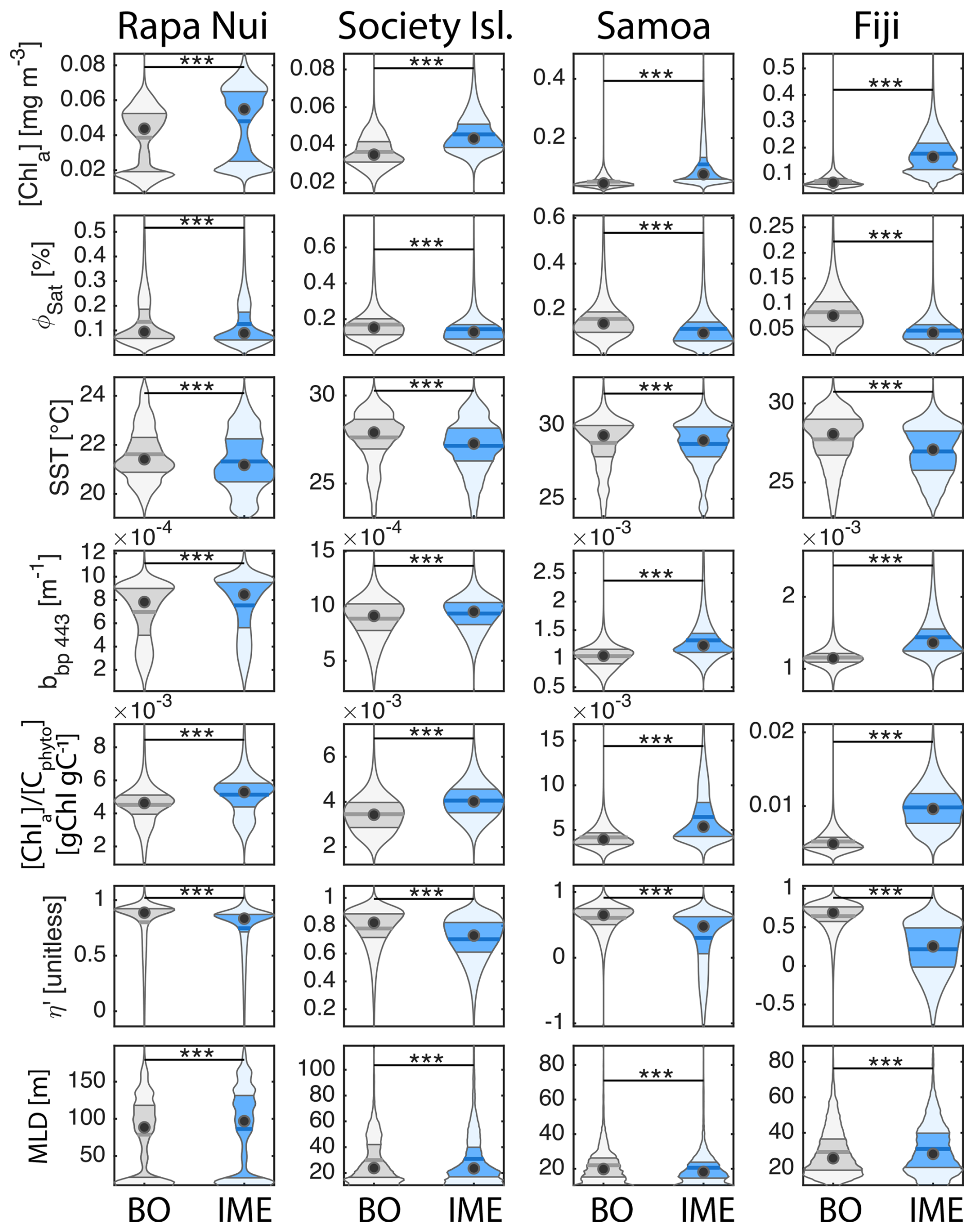
Figure B1 Violin plots chlorophyll a concentration ([Chl a]), backscattering coefficient at 443 nm (b_bp443), ratio of [Chl a] to phytoplankton carbon ($\left[\mathrm{Chl}a\right]/\left[C_{\mathrm{phyto}}\right]$), iron stress index (Φ_Sat; iron stress index), macronutrient stress index (η^′), mixed layer depth (MLD), and sea surface temperature (SST) of all the 2025 IME realizations and their corresponding BO zones showed in Fig. 4. The violin plots show the distribution of all individual pixels of the 8 d median products along the 6-month period studied. The asterisks represent the pairwise significant differences between the studied parameters in IME categories (* $=p<\mathrm{0.05}$, ** $=\mathrm{0.05}⩽p<\mathrm{0.01}$, *** $=\mathrm{0.01}⩽p<\mathrm{0.001}$).

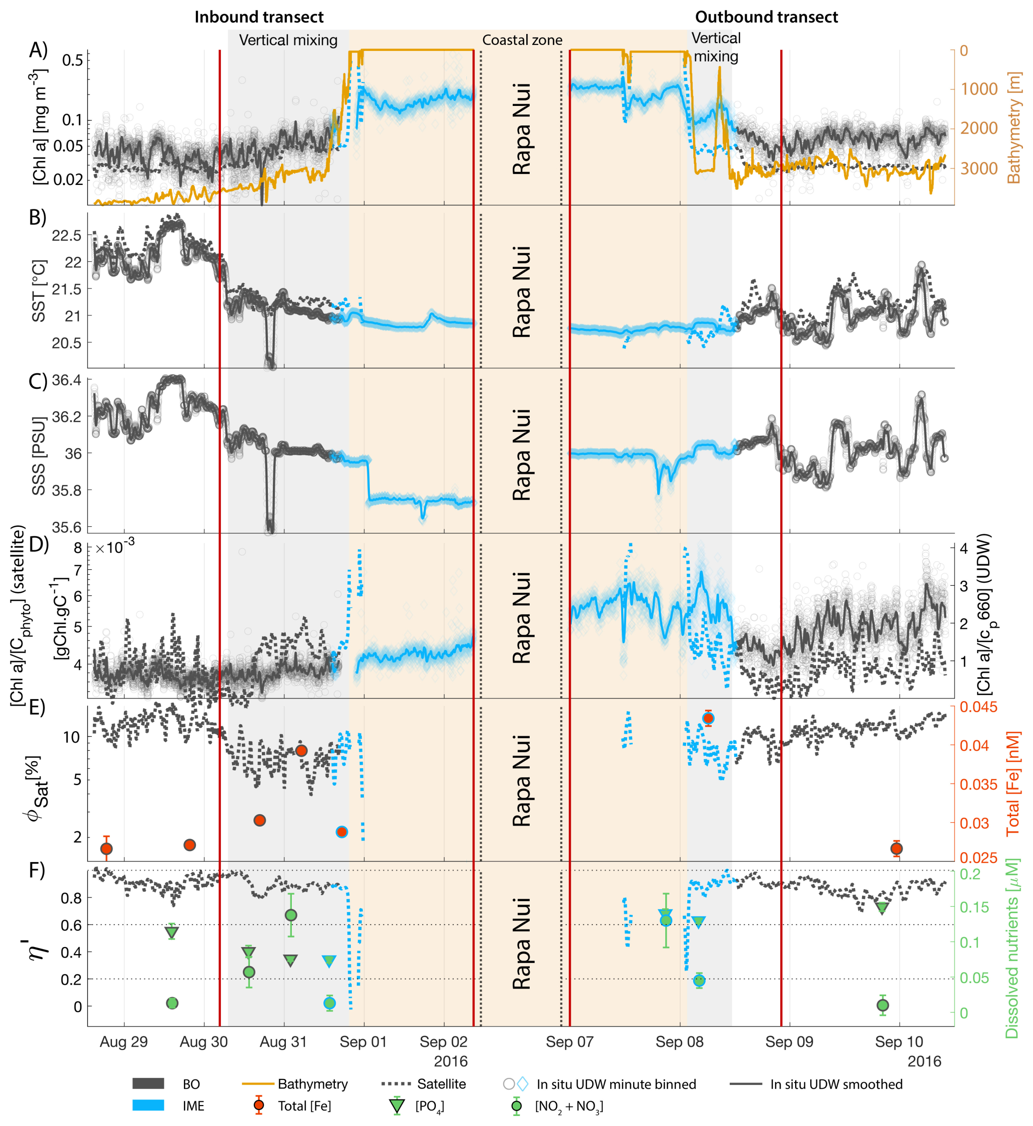
Figure B2 Underway data measured during the inbound (left panels) and outbound (right panels) transects around Rapa Nui and their satellite counterparts, when available. (A) Chlorophyll a concentration ([Chl a]) and bathymetry, (B) sea surface temperature (SST), (C) sea surface salinity (SSS), (D) [Chl a] to phytoplankton carbon ratio from satellite ($\left[\mathrm{Chl}a\right]/\left[C_{\mathrm{phyto}}\right]$) and [Chl a] to beam attenuation at 660 nm from in-situ underway ($\left[\mathrm{Chl}a\right]/c_{\mathrm{p}}\mathrm{660}$), (E) fluorescence quantum yield (Φ_Sat; iron stress index) and total iron concentration measured at sampling stations, (F) macronutrient stress index (η^′) and macronutrient concentrations measured at sampling stations. The blue points show in situ data falling in IME zones detected on the overlapping 8 d satellite composite (BO = black circle, IME = blue diamond). The points show the minute-binned underway data, and the solid lines represent the underway data smoothed with a 2h low-pass digital filter. The gray shaded area highlights the coastal upwelling zone, and the beige shaded area highlights the transect over shallow waters (<100 m depth). The red vertical lines represent the start and end times of the inbound and outbound transect sections shown in Fig. B3.

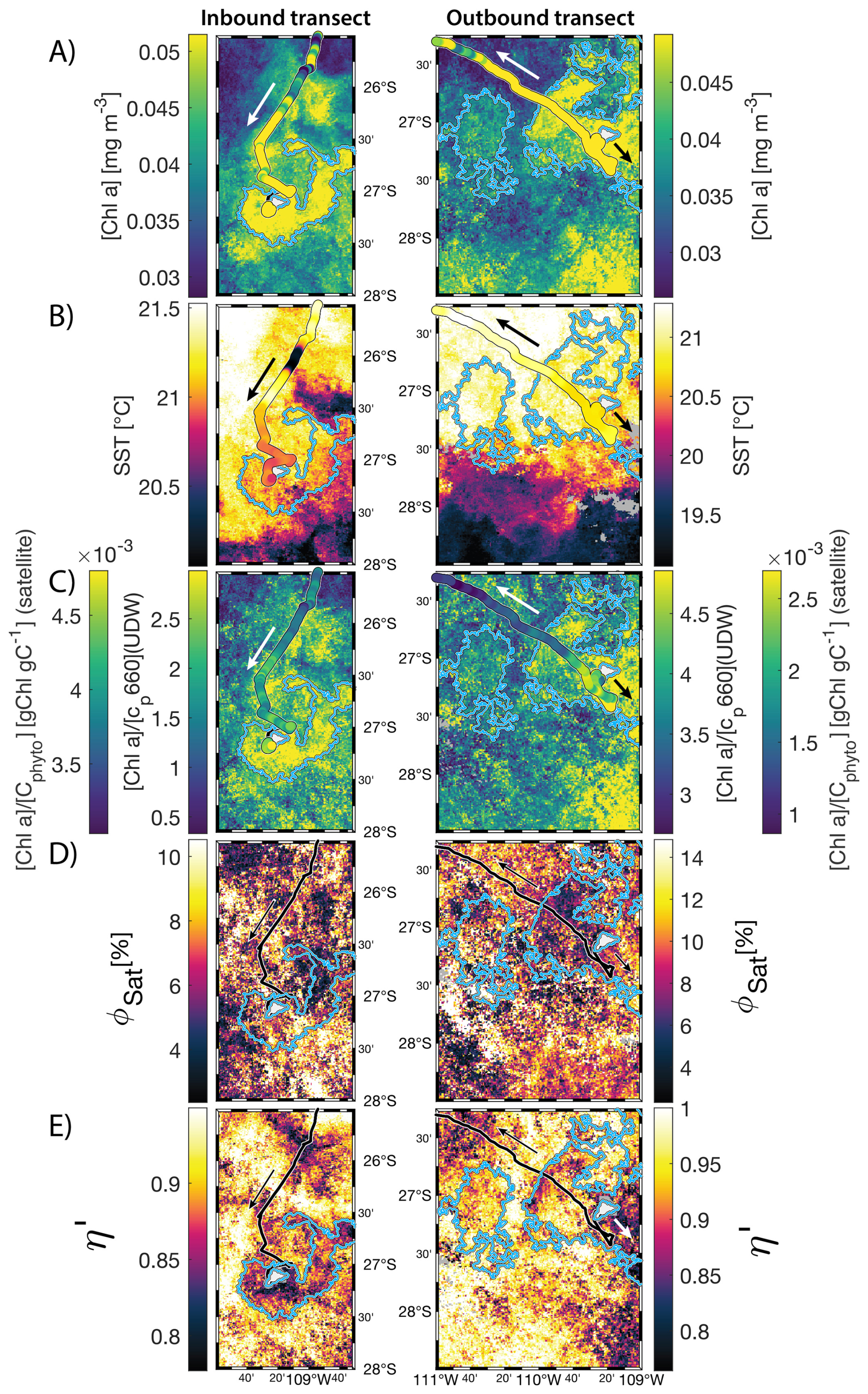
Figure B3 8 d median satellite maps zoomed on the inbound (left-hand-side panels) and outbound transects (right-hand-side panels) around Rapa Nui (arrow shows sailing direction). The blue contour delineates the island mass effect zone detected from satellite chlorophyll a concentration ([Chl a]). In situ underway measurements are overlaid on the satellite map if the same variable was measured from satellite estimates and the underway system. (A) [Chl a], (B) sea surface temperature (SST), (C) [Chl a] to phytoplankton carbon ratio from satellite ($\left[\mathrm{Chl}a\right]/\left[C_{\mathrm{phyto}}\right]$) and [Chl a] to beam attenuation at 660 nm from in-situ underway ($\left[\mathrm{Chl}a\right]/c_{\mathrm{p}}\mathrm{660}$), (D) fluorescence quantum yield (ϕ_Sat; iron stress index), (E) macronutrient stress index (η^′). Entire six-month animated time series accessible in video supplements (Animation S2).

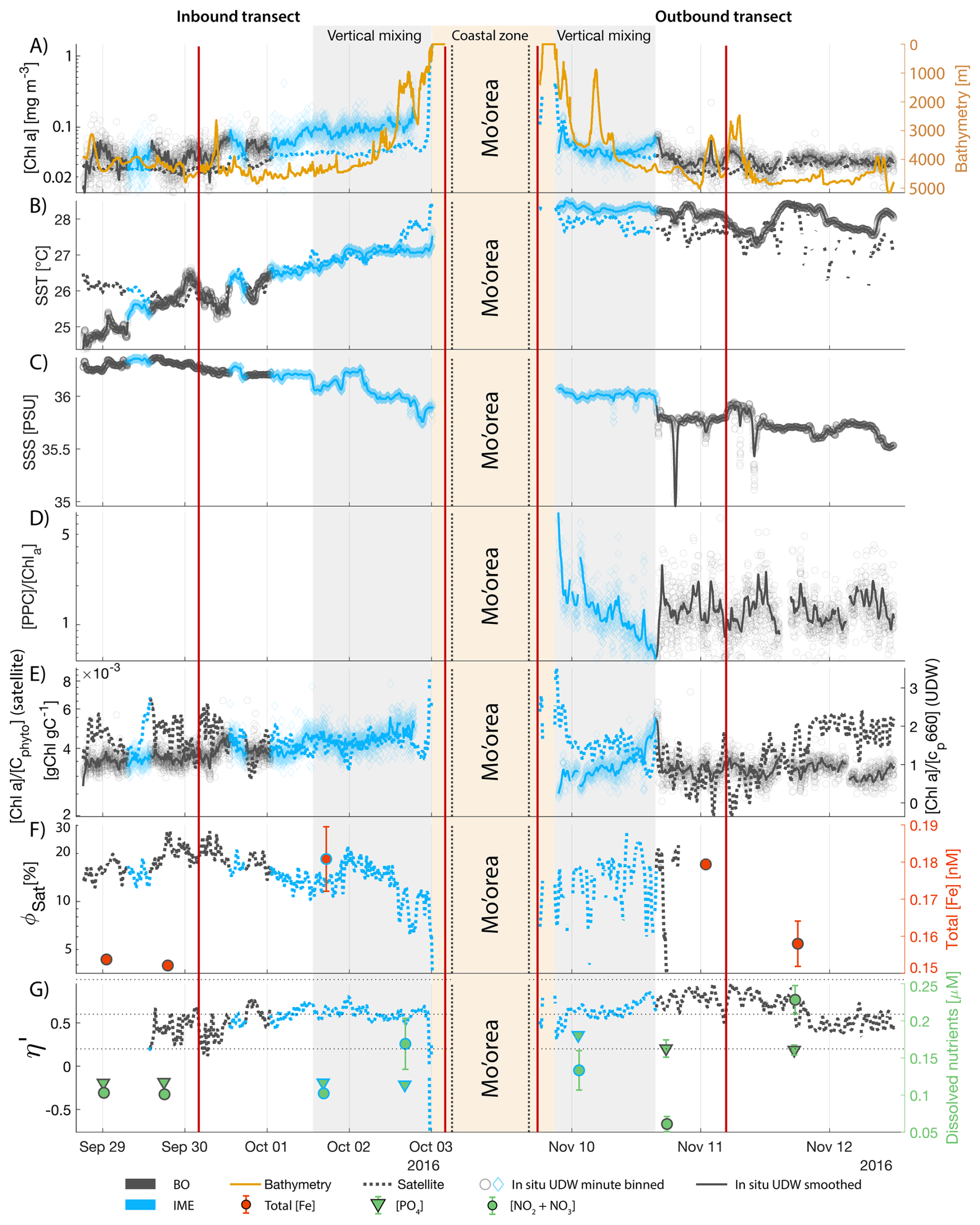
Figure B4 Underway data measured during the inbound (left panels) and outbound (right panels) transects around Society Islands and their satellite counterparts, when available. (A) Chlorophyll a concentration ([Chl a]) and bathymetry, (B) sea surface temperature (SST), (C) sea surface salinity (SSS), (D) Photo-protective carotenoids proportion ($\left[\mathrm{PPC}\right]/\left[\mathrm{Chl}a\right]$), (E) [Chl a] to phytoplankton carbon ratio from satellite ($\left[\mathrm{Chl}a\right]/\left[C_{\mathrm{phyto}}\right]$) and [Chl a] to beam attenuation at 660 nm from in-situ underway ($\left[\mathrm{Chl}a\right]/c_{\mathrm{p}}\mathrm{660}$), (F) fluorescence quantum yield (Φ_Sat; iron stress index) and total iron concentration measured at sampling stations, (G) macronutrient stress index (η^′) and macronutrient concentrations measured at sampling stations. The blue points show in situ data falling in IME zones detected on the overlapping 8 d satellite composite (BO = black circle, IME = blue diamond). The points show the minute-binned underway data, and the solid lines represent the underway data smoothed with a 2 h low-pass digital filter. The gray shaded area highlights the coastal upwelling zone, and the beige shaded area highlights the transect over shallow waters (<100 m depth). The red vertical lines represent the start and end times of the inbound and outbound transect sections shown in Fig. B3.

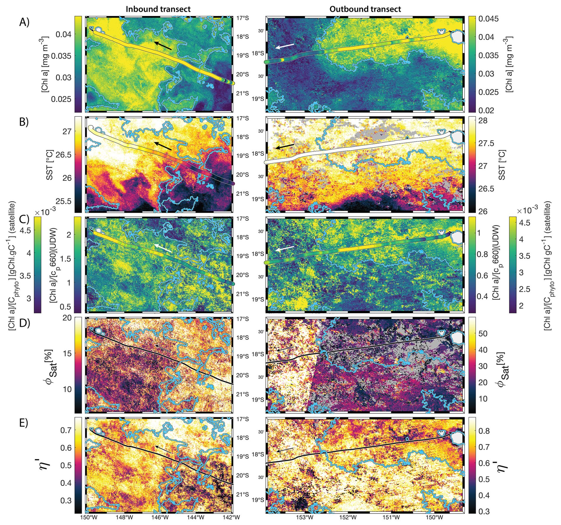
Figure B5 8 d median satellite maps zoomed on the inbound (left-hand-side panels) and outbound transects (right-hand-side panels) around Society Islands (arrow shows sailing direction). The blue contour delineates the island mass effect zone detected from satellite chlorophyll a concentration ([Chl a]). In situ underway measurements are overlaid on the satellite map if the same variable was measured from satellite estimates and the underway system. (A) [Chl a], (B) sea surface temperature (SST), (C) [Chl a] to phytoplankton carbon ratio from satellite ($\left[\mathrm{Chl}a\right]/\left[C_{\mathrm{phyto}}\right]$) and [Chl a] to beam attenuation at 660 nm from in-situ underway ($\left[\mathrm{Chl}a\right]/c_{\mathrm{p}}\mathrm{660}$), (D) fluorescence quantum yield (ϕ_Sat; iron stress index), (E) macronutrient stress index (η^′). Entire six-month animated time series accessible in video supplements (Animation S3).

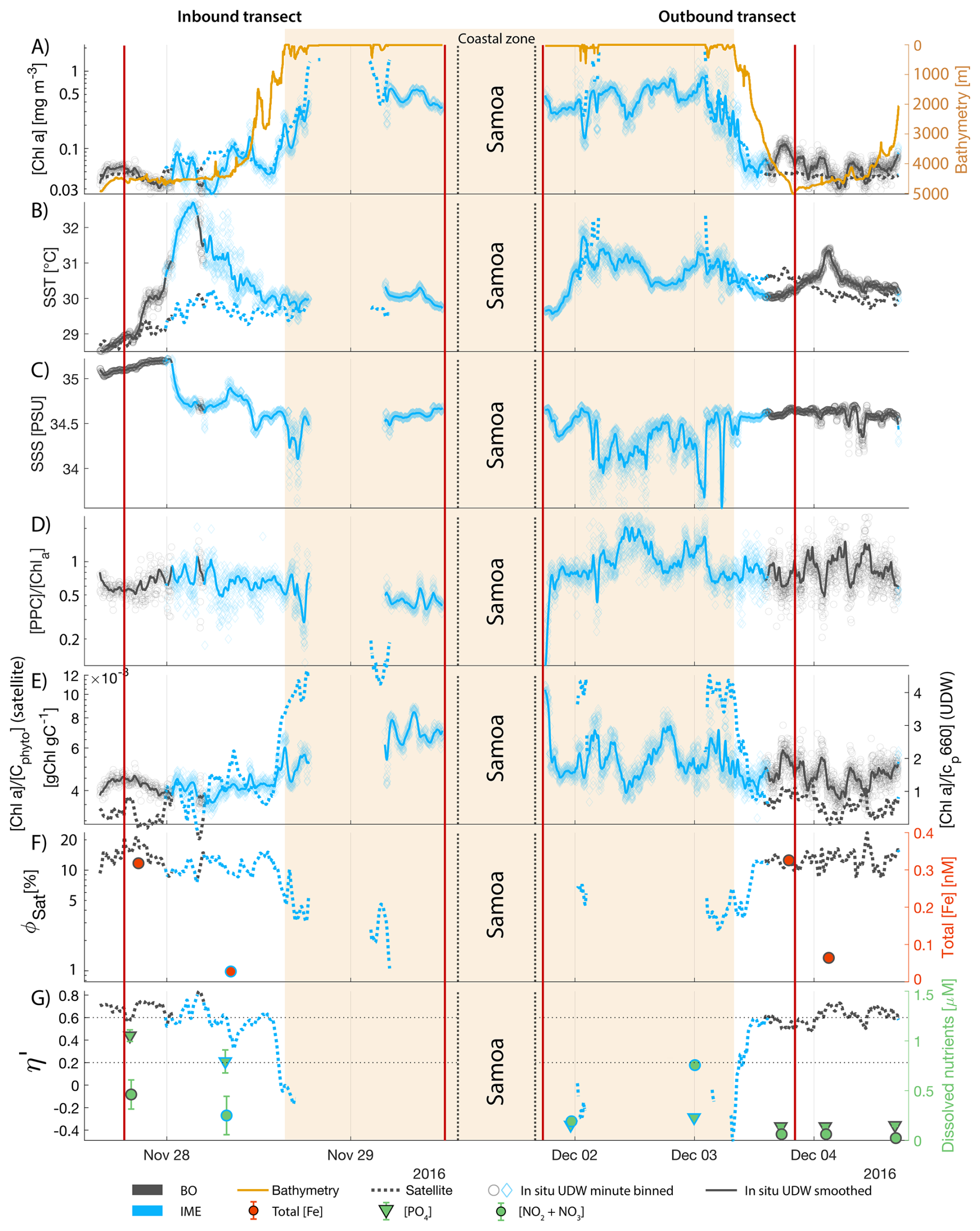
Figure B6 Underway data measured during the inbound (left panels) and outbound (right panels) transects around Samoa and their satellite counterparts, when available. (A) Chlorophyll a concentration ([Chl a]) and bathymetry, (B) sea surface temperature (SST), (C) sea surface salinity (SSS), (D) Photo-protective carotenoids proportion ($\left[\mathrm{PPC}\right]/\left[\mathrm{Chl}a\right]$), (E) [Chl a] to phytoplankton carbon ratio from satellite ($\left[\mathrm{Chl}a\right]/\left[C_{\mathrm{phyto}}\right]$) and [Chl a] to beam attenuation at 660 nm from in-situ underway ($\left[\mathrm{Chl}a\right]/c_{\mathrm{p}}\mathrm{660}$), (F) fluorescence quantum yield (Φ_Sat; iron stress index) and total iron concentration measured at sampling stations, (G) macronutrient stress index (η^′) and macronutrient concentrations measured at sampling stations. The blue points show in situ data falling in IME zones detected on the overlapping 8 d satellite composite (BO = black circle, IME = blue diamond). The points show the minute-binned underway data, and the solid lines represent the underway data smoothed with a 2 h low-pass digital filter. The gray shaded area highlights the coastal upwelling zone, and the beige shaded area highlights the transect over shallow waters (<100 m depth). The red vertical lines represent the start and end times of the inbound and outbound transect sections shown in Fig. B7.

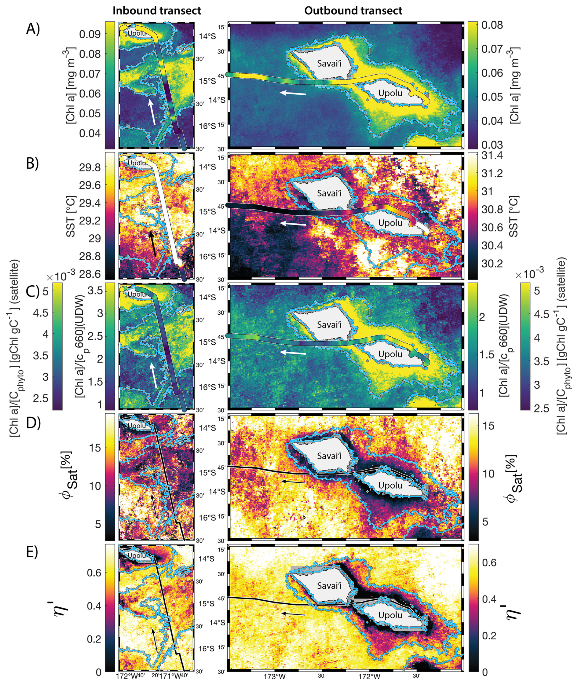
Figure B7 8 d median satellite maps zoomed on the inbound (left-hand-side panels) and outbound transects (right-hand-side panels) around Samoa (arrow shows sailing direction). The blue contour delineates the island mass effect zone detected from satellite chlorophyll a concentration ([Chl a]). In situ underway measurements are overlaid on the satellite map if the same variable was measured from satellite estimates and the underway system. (A) [Chl a], (B) sea surface temperature (SST), (C) [Chl a] to phytoplankton carbon ratio from satellite ($\left[\mathrm{Chl}a\right]/\left[C_{\mathrm{phyto}}\right]$) and [Chl a] to beam attenuation at 660 nm from in-situ underway ($\left[\mathrm{Chl}a\right]/c_{\mathrm{p}}\mathrm{660}$), (D) fluorescence quantum yield (ϕ_Sat; iron stress index), (E) macronutrient stress index (η^′). Entire six-month animated time series accessible in video supplements (Animation S4).

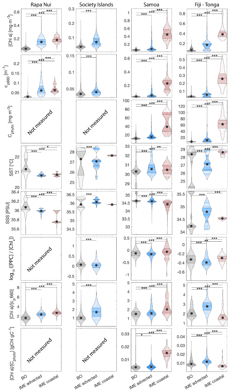
Figure B8 Violin plots of continuous underway data related to phytoplankton concentration and physiology located in the background ocean, advected IME, and coastal IME zones. The four columns represent data measured around the four case studies, while the rows correspond to different phytoplankton community composition parameters: [Chl a] (Chlorophyll a concentration), c_p660 (particulate beam attenuation at 660 nm), C_phyto (phytoplankton carbon), SST (sea surface temperature), SSS (sea surface salinity), $\left[\mathrm{PPC}\right]/\left[\mathrm{Chl}a\right]$ (photoprotective carotenoids normalized by [Chl a]; indicative of light acclimation), $\left[\mathrm{Chl}a\right]/c_{\mathrm{p}\mathrm{660}}$ (proxy of chlorophyll to carbon ratio, indicative of light acclimation), $\left[\mathrm{Chl}a\right]/C_{\mathrm{phyto}}$ (proxy of chlorophyll to carbon ratio, indicative of light acclimation). The asterisks represent the pairwise significant differences between the studied parameters in IME categories (* $=p<\mathrm{0.05}$, ** $=\mathrm{0.05}⩽p<\mathrm{0.01}$, *** $=\mathrm{0.01}⩽p<\mathrm{0.001}$).

Appendix C: Macronutrient and iron concentration

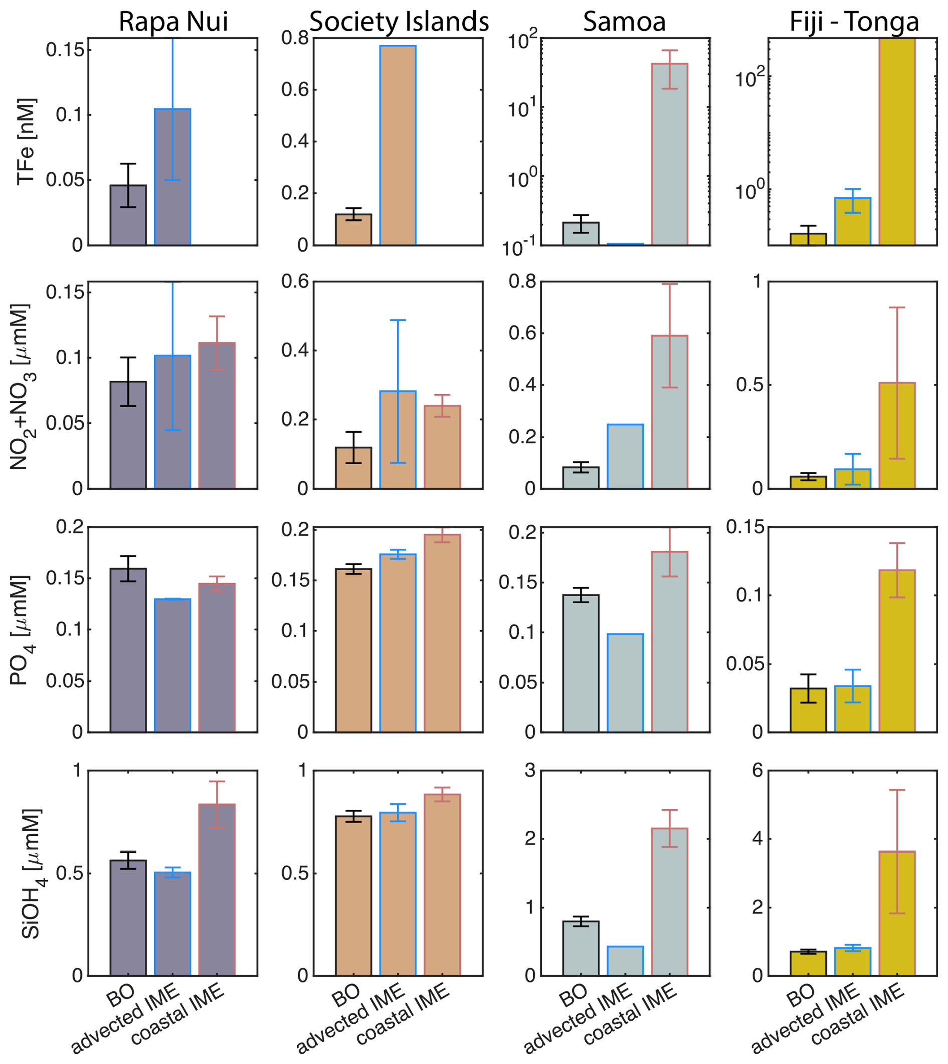
Figure C1 Macronutrient and iron concentrations at sampling stations located in the background ocean, advected IME, and coastal IME zones. The four columns represent data measured around the four case studies, while the rows correspond to different nutrient and trace metal parameters: TFe (total iron), PO₄ (dissolved phosphates), NO₂+NO₃ (dissolved nitrites and nitrate), and SiOH₄ (silicates). The error bars represent the variability (standard error) among all samples within each case study and IME category (BO, advected IME, and coastal IME). A missing error bar indicates that only one sample was available.

Appendix D: Phytoplankton community composition in Rapa Nui, Society Islands, Samoa, and Fiji-Tonga' IMEs

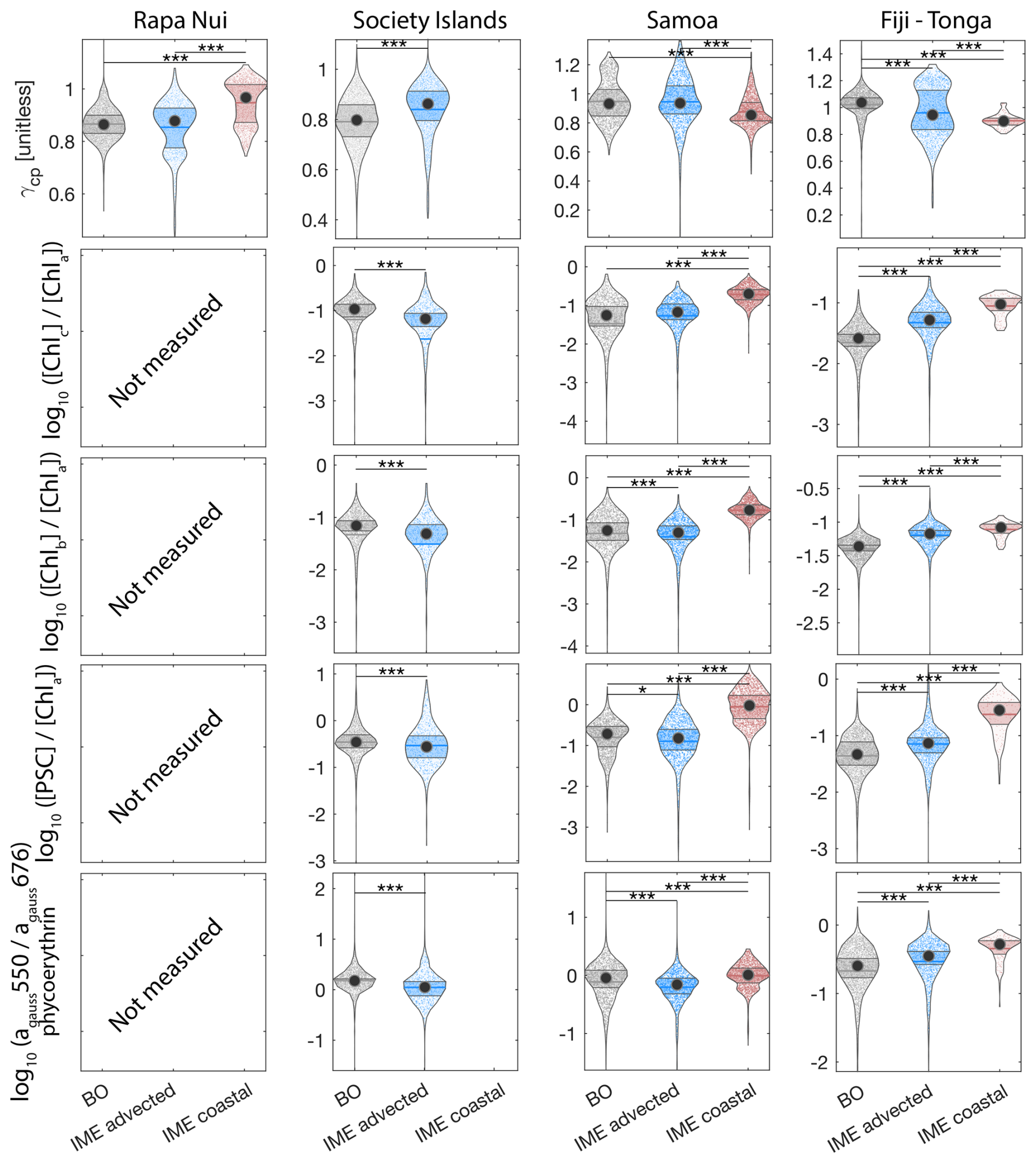
Figure D1 Violin plots of continuous underway data related to phytoplankton community composition located in the background ocean, advected IME, and coastal IME zones. The four columns represent data measured around the four case studies, while the rows correspond to different phytoplankton community composition parameters: ${\mathit{\gamma }}_{c_{\mathrm{p}}}$ (mean particle size index), $\left[\mathrm{Chl}c\right]/\left[\mathrm{Chl}a\right]$ (Chlorophyll c normalized by [Chl a]; indicative of diatoms and other red algae), $\left[\mathrm{Chl}b\right]/\left[\mathrm{Chl}a\right]$ (Chlorophyll b normalized by [Chl a]; indicative of green algae), $\left[\mathrm{PSC}\right]/\left[\mathrm{Chl}a\right]$ (photosynthetic carotenoids normalized by [Chl a]; indicative of diatoms), and $a_{\mathrm{gauss}}\mathrm{550}/a_{\mathrm{gauss}}\mathrm{676}$ (Phycoerythrin particulate gaussian absorption at 550 nm normalized by [Chl a] particulate gaussian absorption at 676 nm; indicative of cyanobacteria).The asterisks represent the pairwise significant differences between the studied parameters in IME categories (* $=p<\mathrm{0.05}$, ** $=\mathrm{0.05}⩽p<\mathrm{0.01}$, *** $=\mathrm{0.01}⩽p<\mathrm{0.001}$).

Appendix E: Temporal analysis of IME around Rapa Nui, Society Islands, and Samoa

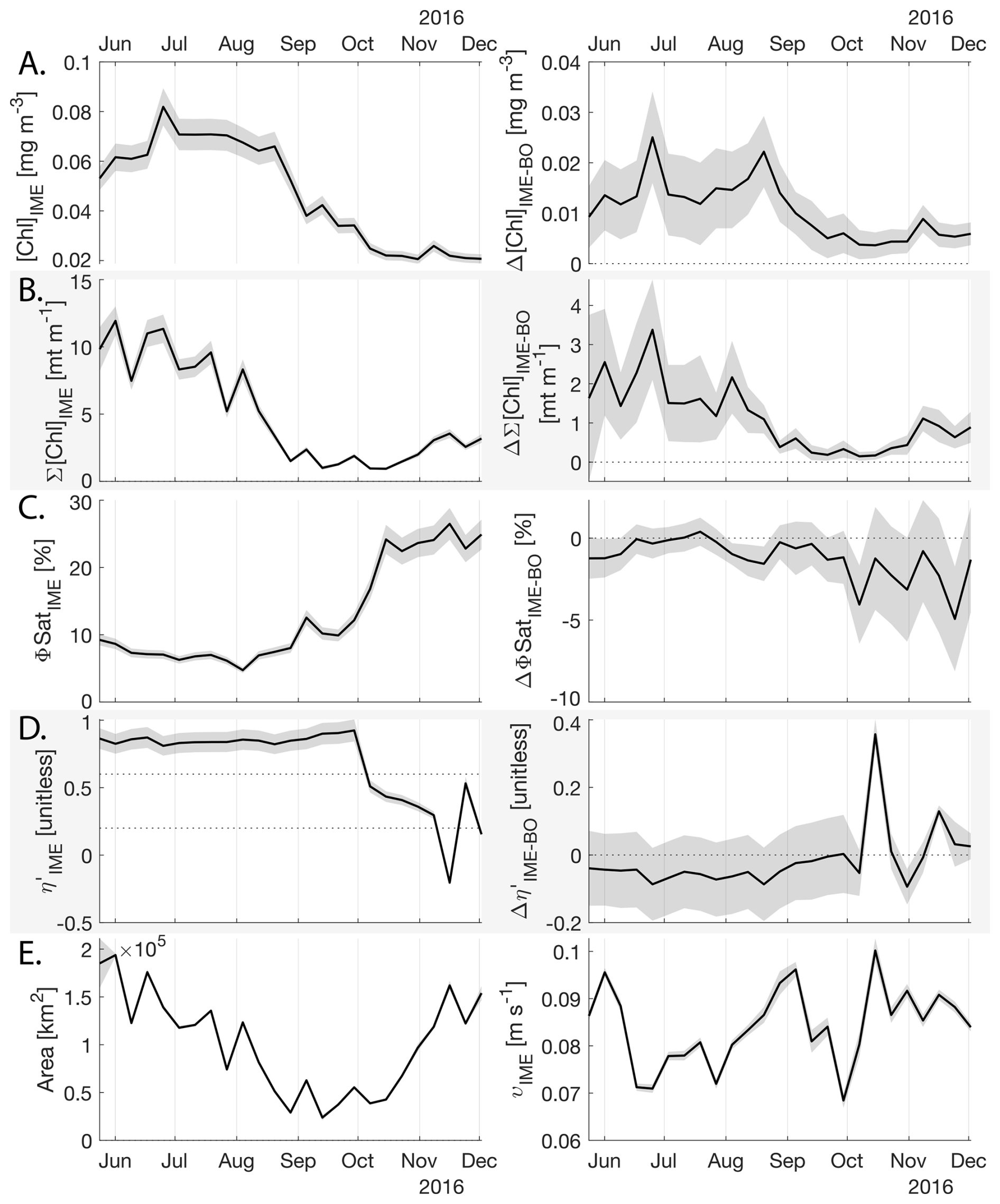
Figure E1 Six-month-long time series of satellite-derived IME properties of the IME zone detected around Rapa Nui. (A), (B), (C), and (D) left panels: Average of properties within the IME zones, (A), (B), (C), and (D) right panels: Difference between properties within the IME zones and the background ocean (BO). (A) row: chlorophyll a concentration ([Chl a]), (B) row: IME integrated chlorophyll a (∑[Chl a]_IME), (C) row: fluorescence quantum yield (ϕ_Sat; iron stress index), (D) row: macronutrient stress index (η^′), (E) left: IME zone area (in km²), (E) right: surface current velocity. The shaded areas represent the standard errors propagated following the method in Appendix A4.

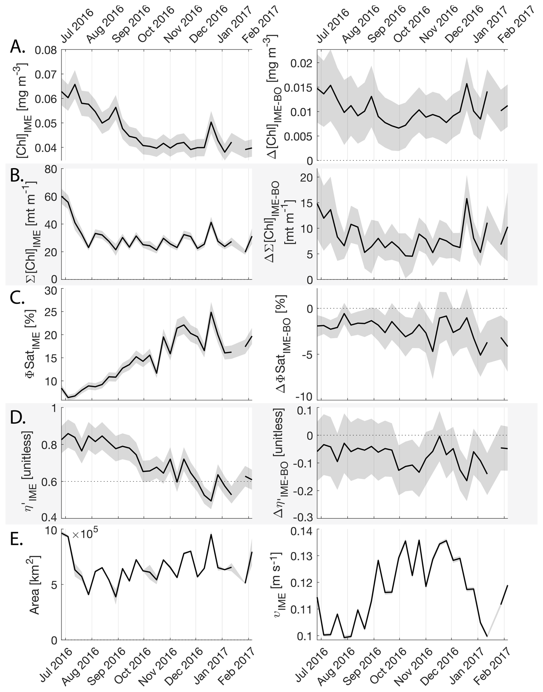
Figure E2 Six-month-long time series of satellite-derived IME properties of the IME zone detected around the Society Islands in French Polynesia. (A), (B), (C), and (D) left panels: Average of properties within the IME zones, (A), (B), (C), and (D) right panels: Difference between properties within the IME zones and the background ocean (BO). (A) row: chlorophyll a concentration ([Chl a]), (B) row: IME integrated [Chl a] (∑[Chl a]_IME), (C) row: fluorescence quantum yield (ϕ_Sat; iron stress index), (D) row: macronutrient stress index (η^′), (E) left: IME zone area (in km²), (E) right: surface current velocity. The shaded areas represent the standard errors propagated following the method in Appendix A4.

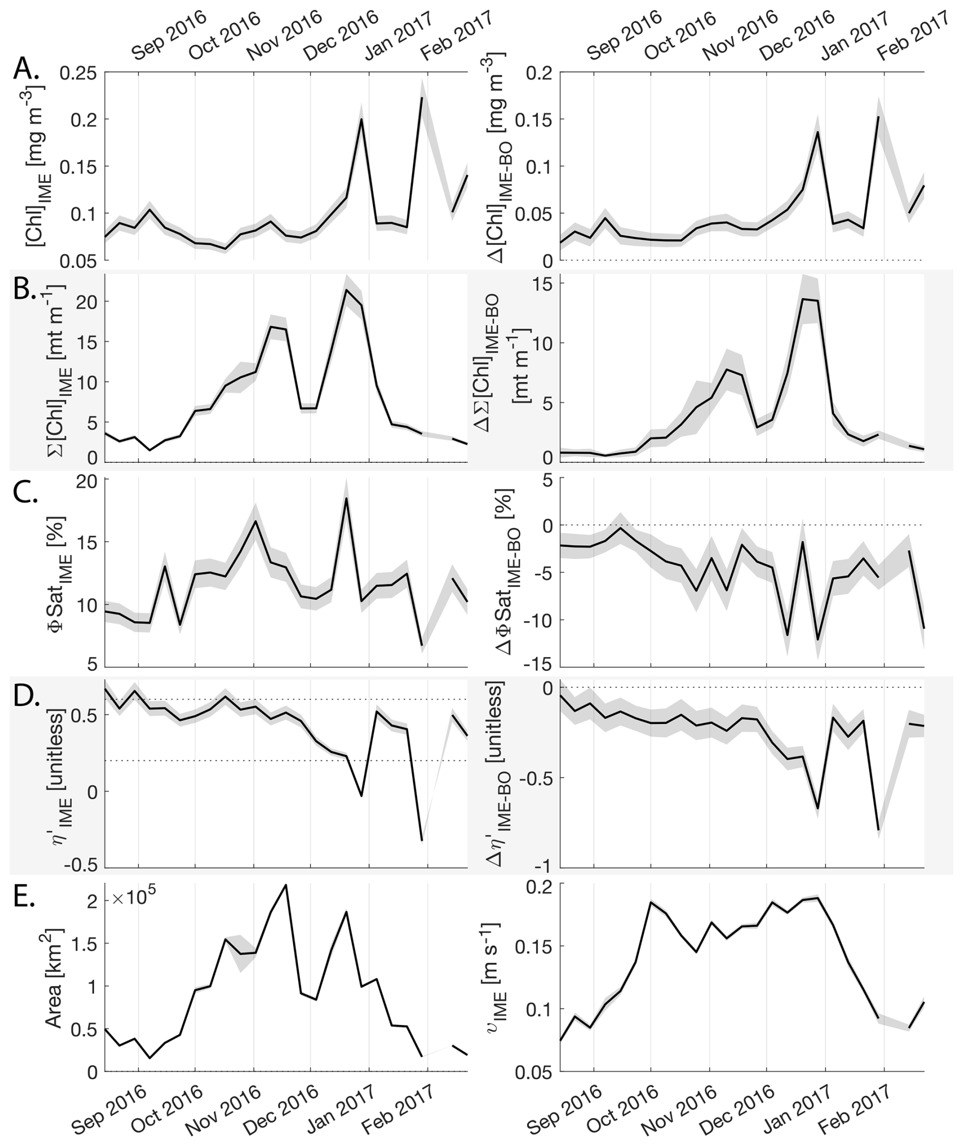
Figure E3 Six-month-long time series of satellite-derived IME properties of the IME zone detected around Samoa (Savaii, Upolu, and Tutuila). (A), (B), (C), and (D) left panels: Average of properties within the IME zones, (A), (B), (C), and (D) right panels: Difference between properties within the IME zones and the background ocean (BO). (A) row: chlorophyll a concentration ([Chl a]), (B) row: IME integrated [Chl a] (∑[Chl a]_IME), (C) row: fluorescence quantum yield (ϕ_Sat; iron stress index), (D) row: macronutrient stress index (η^′), (E) left: IME zone area (in km²), (E) right: surface current velocity. The shaded areas represent the standard errors propagated following the method in Appendix A4.