A top-down evaluation of bottom-up estimates to reduce uncertainty in methane emissions from Arctic wetlands

Wetlands are a major natural source of atmospheric CH₄, however, accurately estimating their emissions is difficult due to the complex biogeochemical interactions and spatial heterogeneity of wetland environments. This study explores how a combination of atmospheric inverse and process-based modelling can reduce the discrepancy in Arctic wetland estimates between bottom-up and top-down approaches. We employed the Jena CarboScope global inversion system, incorporating prior wetland fluxes simulated by the JSBACH land surface model, which is part of the Max Planck Institute Earth System Model (MPI-ESM). We conducted a series of inversion experiments, each incorporating JSBACH-generated CH₄ fluxes based on different CH₄ production Q₁₀ values, which represents the temperature dependence of CH₄ production. Additionally, we examined the impact of changing the baseline $f_{{\mathrm{CH}}_{\mathrm{4}}}$ fraction value, which defines the fraction of anaerobically mineralized carbon converted to CH₄, while keeping all other JSBACH and inversion settings constant. Our findings show that, at a pan-Arctic scale, using a CH₄ Q₁₀ value of 1.8 produces the best agreement between the two approaches. However, no single Q₁₀ value yielded optimal agreement between the simulated fluxes and the fluxes inferred from atmospheric observations across all subregions. Instead, the best performance varied spatially, with different CH₄ production Q₁₀ values and baseline $f_{{\mathrm{CH}}_{\mathrm{4}}}$ fraction leading to a better flux agreement in specific areas. These results highlight the importance of using regionally specific parameters to more accurately estimate wetland CH₄ emissions, and the potential of employing atmospheric inversions to guide bottom-up process models towards regionally representative parameter settings.

1 Introduction

Methane (CH₄) is the second most important anthropogenic greenhouse gas and it is emitted from both natural and anthropogenic sources. Combined wetlands and inland freshwaters are the largest natural source of CH₄ to the atmosphere, accounting for about 28 %–37 % (by bottom-up and top-down estimates, respectively) of the global total CH₄ emissions (Saunois et al., 2025). However, quantifying these emissions remains challenging due to the complexity of biogeochemical processes and the spatial variability of these ecosystems. Constraining CH₄ budgets is particularly relevant in the Arctic–Boreal region, which is warming faster than most other regions (Rantanen et al., 2022), and at the same time contains extensive wetlands and permafrost landscapes storing significant amounts of soil carbon (Hugelius et al., 2024). Under warming conditions, this carbon can be mobilized and potentially release substantial amounts of CH₄ into the atmosphere. Large uncertainties in Arctic CH₄ emission estimates limit our ability to quantify the region's contribution to the global CH₄ budget and its climate feedbacks.

Global and regional CH₄ emissions are estimated using both bottom-up or top-down approaches. Bottom-up methods, including inventories, data-driven ecosystem flux upscaling and process-based models, provide detailed information with fine-scale resolution for both, processes and spatial heterogeneity. Process-based models simulate CH₄ emissions by mathematically representing ecosystem dynamics, biogeochemical cycles, and physical processes. However, extrapolating these estimates to regional or global scales is challenging due to the strong spatial variability in wetland characteristics (e.g., extent, hydrology and vegetation), as well as sensitivity of the models to parameterizations. Top-down approaches estimate net surface–atmosphere CH₄ fluxes using atmospheric observations (in situ, flask and/or satellite measurements) in combination with prior flux information (from process-based models and/or inventories), and atmospheric transport and chemistry models to link surface sources with atmospheric observations. Their ability to provide accurate estimates of net surface–atmosphere fluxes is limited by sparse observational coverage, particularly in remote regions, as well as by uncertainties in atmospheric transport, prior flux estimates, and atmospheric CH₄ sink processes (Houweling et al., 2017). These limitations can lead to significant uncertainties in the magnitude and spatial distribution of inferred emissions, which makes attributing fluxes to specific sources or processes challenging. Still, despite these limitations, the inverse modeling approach allowed us to derive important constraints on the global sources and sinks of CH₄ (Houweling et al., 2017).

Although both approaches are widely used, substantial discrepancies exist between bottom-up and top-down estimates of CH₄ emissions. From 2010 to 2019, top-down approaches estimated global CH₄ emissions at 575 Tg CH₄ yr⁻¹ (553–586 Tg CH₄ yr⁻¹), whereas bottom-up estimates were approximately 15 % higher, at 669 Tg CH₄ yr⁻¹ (512–849 Tg CH₄ yr⁻¹) (Saunois et al., 2025). Similar differences are evident in the high-northern latitudes regions, where wetlands and inland waters dominate emissions. In the Arctic–Boreal region, bottom-up estimates of 50 Tg CH₄ yr⁻¹ (29–71 Tg CH₄ yr⁻¹) contrast with top-down estimates of 20 Tg CH₄ yr⁻¹ (15–24 Tg CH₄ yr⁻¹) (Hugelius et al., 2024).

Mechanistic modeling of net surface CH₄ emissions requires capturing a range of complex, interacting processes (Conrad, 1999; Moser et al., 2026; Riley et al., 2011). As a key parameter, the net CH₄:CO₂ production ratio is determined by the relative importance of several biogeochemical processes, which in turn are dependent on environmental conditions, and a large range of this production ratio has been observed (Knoblauch et al., 2018). As a consequence, global-scale land surface models often represent anaerobic CH₄ production in a simplified way, i.e. as a first-order decay of soil organic matter with adjusted rate constants, applying a fixed ratio of CH₄ versus CO₂ production (Guimberteau et al., 2018; Kleinen et al., 2020; Moser et al., 2026; Ricciuto et al., 2021; Sellar et al., 2019). Here, the models can differ in whether the ratio applies to the CH₄ production or emission.

Biogeochemical process models require balancing the inclusion of key mechanisms with limitations such as structural and parameter uncertainty, spatial heterogeneity, sparse observational data, uncertain initial and boundary conditions, and computational constraints (Riley et al., 2011). Regarding the simulation of CH₄ emissions, a higher CH₄:CO₂ ratio indicates a greater dominance of CH₄ in production and emission relative to CO₂ (Chinta et al., 2024), while a higher CH₄ production Q₁₀ indicates that CH₄ production increases more rapidly with rising temperatures. As regional model sensitivity varies and site-specific measurements may not be representative across broader areas, both the CH₄:CO₂ ratio and the CH₄ production Q₁₀ are uncertain at large spatial scales. For example, increasing CH₄ production Q₁₀ in high-latitude regions can reduce simulated CH₄ emissions by more than half, because the temperature-dependent component, scaled relative to a reference temperature of 295 K, leads to a decline in CH₄ production rate at the lower temperatures typical of these regions (Riley et al., 2011). As many large-scale land surface models still rely on simplified, fixed CH₄ production fractions, their ability to accurately represent observed spatiotemporal variability in CH₄:CO₂ production ratios across Arctic landscapes is therefore limited (Moser et al., 2026). These differences in model structure, parameterization and initialization contribute strongly to relative high uncertainties in wetland estimates (Poulter et al., 2017).

The JSBACH v3.2 model (Reick et al., 2021) that we apply in this study is taking the first approach and mechanistically distinguish between methanogenesis and methanotrophy. In JSBACH v3.2, anaerobic decomposition and CH₄ oxidation are temperature dependent and the CH₄:CO₂ production ratio is also assumed to follow a Q₁₀ temperature sensitivity (Kleinen et al., 2020). This formulation allows the relative importance of the above-mentioned underlying biogeochemical processes changes in space and time depending on the soil temperature. In addition, making the CH₄:CO₂ production ratio temperature dependent allows us to additionally tune CH₄ versus CO₂ production across bioclimatic zones. Still, the optimum parameter setting of the Q₁₀ value for this temperature dependency of the CH₄:CO₂ production ratio is still highly uncertain.

This study therefore explores novel concepts for using atmospheric inverse modeling to constrain parameter settings in bottom-up estimates of wetland CH₄ emissions in the Arctic–Boreal region. Using the Jena CarboScope global inversion system, we employed prior fluxes from the JSBACH land surface model (a component of the MPI Earth System Model) and systematically varied key parameters that govern CH₄ production. Specifically, we tested a range of Q₁₀ values, which define the temperature sensitivity of CH₄ production, and different $f_{{\mathrm{CH}}_{\mathrm{4}}}$ baseline values, which determine the proportion of anaerobically mineralized carbon converted to CH₄. However, a portion of the produced CH₄ is oxidized to CO₂. Since transport pathways determine how much CH₄ is exposed to oxidation on its way to the surface, they reduce the resulting CH₄:CO₂ emission ratio. We kept other model settings constant throughout these tests. Integrating these parameter sensitivity experiments into the inversion framework allowed us to assess which parameterizations yield the most consistent fluxes with atmospheric observations. This approach enables us to identify regionally representative parameter settings and guide parameterizations that could improve the consistency between bottom-up process models and top-down constraints on Arctic–Boreal wetland CH₄ emissions.

2 Methods

2.1 Region and time period of interest

Our Arctic–Boreal domain was defined based on The Boreal–Arctic Wetland and Lake Dataset – BAWLD (Olefeldt et al., 2021), and we divided this region into 6 sub-regions for more detailed spatial analyses (Alaska, western Canada, eastern Canada, Europe including Greenland, western Russia, eastern Russia, Fig. 1). In recent decades, the atmospheric observation network suitable for inverse modeling has expanded across the Arctic, with a considerable increase in available sites after 2010 (Vogt et al., 2025). However, due to data-sharing disruptions associated with the ongoing conflict involving Russia and Ukraine, observational data from Russian stations has been limited since 2022. Consequently, this study focuses on the period from 2010 to 2021, when data coverage from surface stations was more consistent across the full domain.

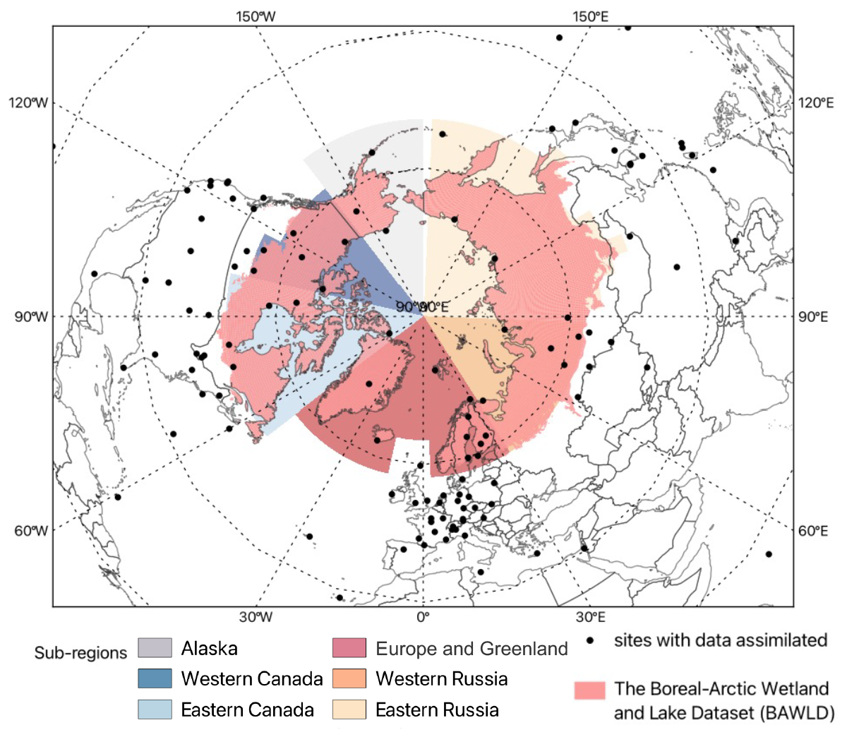
Figure 1 Geographic distribution of surface sites operated by different network providers where flask-based and/or continuous in-situ CH₄ measurements are available for assimilation into the inverse model (black dots; Table S1 in the Supplement). The colored boxes delineate the Arctic–Boreal regions (Alaska, western Canada, eastern Canada, Europe including Greenland, western Russia, eastern Russia), as defined based on The Boreal–Arctic Wetland and Lake Dataset (BAWLD) (Olefeldt et al., 2021).

2.2 Wetland estimates used as prior fluxes in the inverse modelling

In this study, we utilize the JSBACH model (Reick et al., 2021), the land component of the MPI-ESM (Mauritsen et al., 2019), to estimate bottom-up wetland CH₄ emissions. JSBACH is run in standalone mode at T63 resolution (approximately 1.85°, or 185 km) and driven by CRUJRA2.3 (Harris, 2019) climate forcing. Soil hydrology and thermodynamics follow the multilayer formulation of Hagemann and Stacke (2015), with permafrost-related processes implemented as described by Ekici et al. (2014). Soil organic carbon (SOC) decomposition is simulated as a first-order decay process that depends on surface air temperature, water availability, and litter size, following the YASSO model formulation (Tuomi et al., 2011) and its implementation in JSBACH by Goll et al. (2015).

The wetland area fraction of the grid is determined using TOPMODEL (Beven and Kirkby, 1979), a conceptual rainfall–runoff model that estimates inundation based on the compound topographic index (CTI). If the inundated fraction of the grid is non-frozen (depending on the soil temperature), it is considered a CH₄-emitting area. The methodology for wetland CH₄ production and transport is adopted from Riley et al. (2011), and the details of the TOPMODEL and its implementation for wetland CH₄ within JSBACH are outlined in Kleinen et al. (2020).

Methane production and the transport pathways that move CH₄ to the surface (diffusion, plant-mediated aerenchyma and ebullition) follow the scheme of Riley et al. (2011), as implemented in JSBACH by Kleinen et al. (2020). Under anaerobic conditions, a proportion of SOC ($f_{{\mathrm{CH}}_{\mathrm{4}}}$) is converted to CH₄, while the remaining is converted to CO₂. The temperature dependence of $f_{{\mathrm{CH}}_{\mathrm{4}}}$ is represented using a Q₁₀ formulation.

$$\begin{array}{}\text{(1)}& f_{{\mathrm{CH}}_{\mathrm{4}}}=f_{{\mathrm{CH}}_{\mathrm{4}}\text{,baseline}}\cdot {\mathrm{Q}}_{\mathrm{10}}^{(T_{\text{soil}}-\mathrm{295})/\mathrm{10}K}\end{array}$$

Oxidation reduces the amount of CH₄ that reaches the atmosphere. Consequently, the net CH₄:CO₂ emission ratio depends on production and oxidation rates, as well as transport pathways, which control the amount of CH₄ exposed to oxidation. A simplified conceptual relationship is as follows:

$$\begin{array}{}\text{(2)}& {\mathrm{CH}}_{\mathrm{4}}:{\mathrm{CO}}_{\mathrm{2}}={\displaystyle \frac{f_{{\mathrm{CH}}_{\mathrm{4}}}P-O_{{\mathrm{CH}}_{\mathrm{4}}}}{(\mathrm{1}-f_{{\mathrm{CH}}_{\mathrm{4}}})P+O_{{\mathrm{CH}}_{\mathrm{4}}}}}\end{array}$$

where P is gross anaerobic SOC decomposition and O is the amount of CH₄ oxidized before emission.

To evaluate how sensitive CH₄ wetland emission estimates are to key parameters, we conducted nine experiments in which we varied only the Q₁₀ coefficient for CH₄ production and the baseline $f_{{\mathrm{CH}}_{\mathrm{4}}}$ fraction (Fig. 2b). Specifically, we tested three different Q₁₀ values ranging from 1.4 to 2.2, consistent with commonly used values reported in literature review (Moser et al., 2026), and baseline $f_{{\mathrm{CH}}_{\mathrm{4}}}$ fractions from 0.33 to 0.38. These combinations are summarized in Table 1 and were chosen to identify parameter sets that best align with the observed atmospheric data. All other carbon decomposition, hydrological, transport, and oxidation processes follow the standard JSBACH configuration.

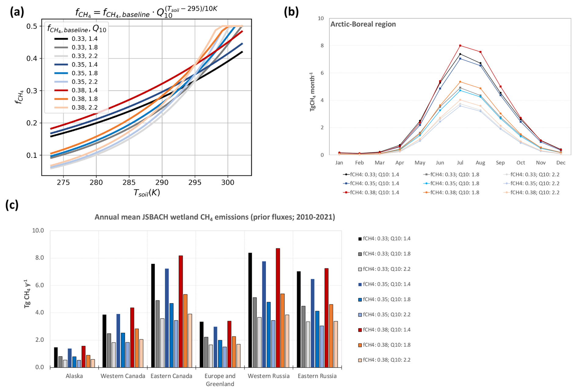
Figure 2 (a) Sensitivity of $f_{{\mathrm{CH}}_{\mathrm{4}}}$ production fraction to the chosen range of input parameters for this study. The y axis represents the fraction of anaerobic carbon mineralization allocated to CH₄ production, calculated using the equation displayed at the top of the panel and in Eq. (1). In the legend, the first number denotes the $f_{{\mathrm{CH}}_{\mathrm{4}}}$ baseline fraction and the second number denotes the CH₄ production Q₁₀ value. (b) Mean seasonal cycle of Arctic–Boreal wetland CH₄ emissions for each experiment used in the inversion as the wetland prior flux. (c) Annual mean wetland fluxes from each experiment estimated by JSBACH model.

Table 1 Summary of JSBACH wetland CH₄ estimates used as prior fluxes in the inversions and posterior fluxes estimates for each respective model run.

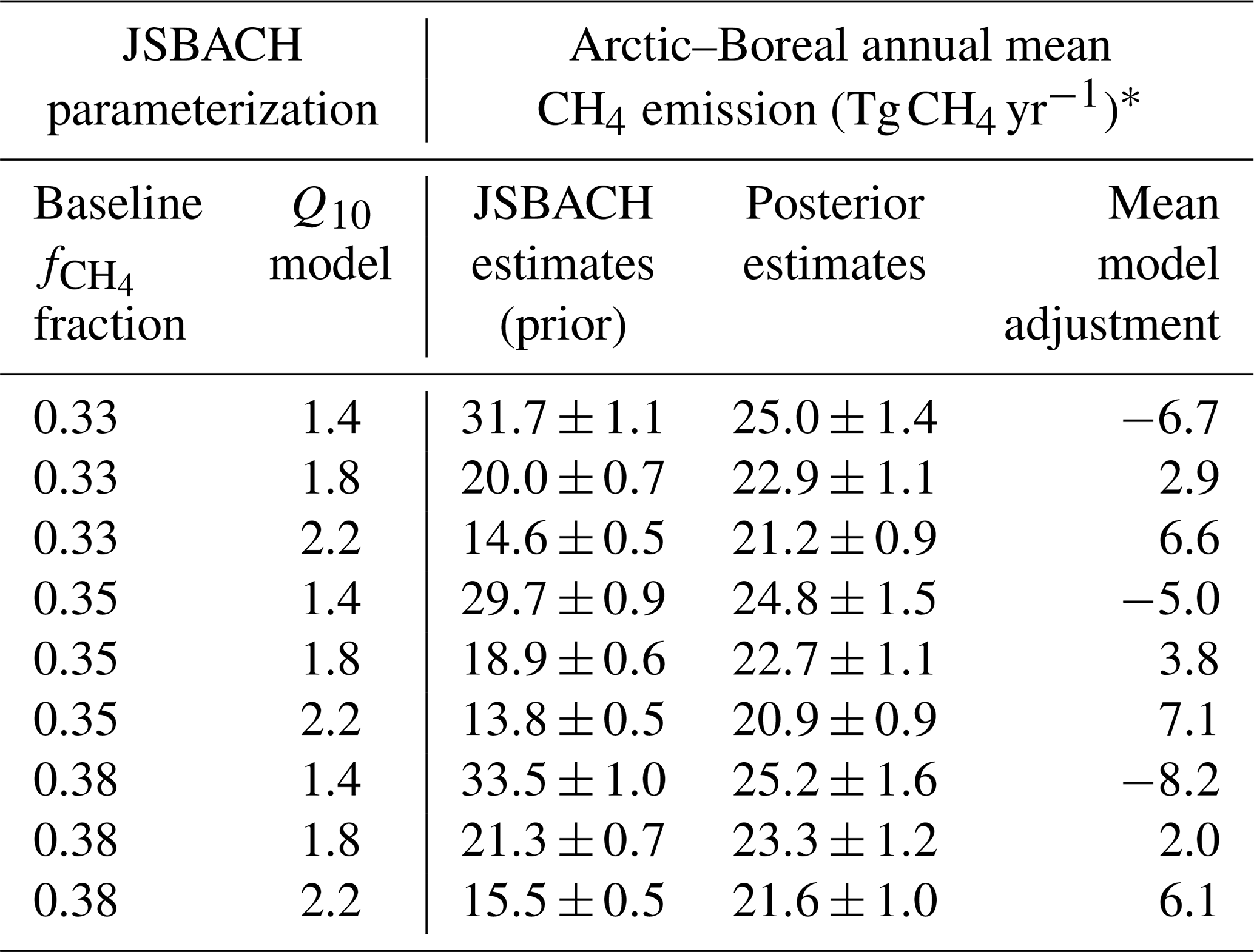
^∗ The annual mean between 2010 and 2021, with the standard deviation representing interannual variability.

2.3 Inverse modeling setup

We used the Jena CarboScope Inversion System (Rödenbeck, 2005) to quantify CH₄ emissions between the surface and the atmosphere globally from 2010 to 2021, with the evaluation and interpretation of fluxes focused on the Arctic–Boreal region. This is a linear Bayesian framework that infers surface–atmosphere CH₄ fluxes by combining prior flux estimates with atmospheric CH₄ mole fraction measurements and accounting for their respective uncertainties. The flux vector f represents the net flux per grid cell per time step. The Jena CarboScope enables f to be represented as the sum of different flux components, each of which is modelled independently using its own statistical linear flux model. These independent a priori error covariance structures allow deviations from the prior flux estimate to be attributed to specific components during the inversion process. In this study, the a priori shape uncertainty was defined as 100 % of the prior flux for each flux category. All flux categories were optimized, assuming spatial correlation lengths of ∼500 km and temporal correlation lengths of about 15 d. Temporal and spatial fluxes are optimized within a Bayesian inversion framework that minimizes a cost function combining prior and observational constraints. The solution is obtained analytically using the linear Bayesian approach, which yields maximum posterior flux estimates and their associated uncertainties. Details of the cost function formulation and solution method can be found in the CarboScope technical report (Rödenbeck, 2005).

A total of 154 stations were assimilated for the global domain (Fig. 1, Table S1). These CH₄ observations were obtained from multiple global and regional networks (ICOS RI et al., 2024; Panov et al., 2021; Sasakawa et al., 2010, 2025; Schuldt et al., 2023), with the majority of sites located in the Northern Hemisphere, including 33 stations within the Arctic–Boreal domain. Most observational data used in this study were accessed through NOAA GML ObsPack (Schuldt et al., 2023), ICOS Carbon Portal (ICOS RI et al., 2024), World Data Centre for Greenhouse Gases (WDCGG) database (https://doi.org/10.50849/WDCGG_CH4_ALL_2023; Dinoi et al., 2023), and JR-STATION network (Sasakawa et al., 2010, 2025); further details are provided in the “Data Availability section”. Detailed information on the stations with assimilated data is given in Table S1. For tower sites with multiple intake heights available, we assimilated only data from the highest height in the inversion, and for the continuous data, we use only daytime measurements. The transport model used in CarboScope is the TM3 global atmospheric tracer model, an Eulerian transport model that solves the continuity equation (and parameterizations of boundary layer and convective mixing) for atmospheric tracers in a three-dimensional grid over the globe (Heimann and Körner, 2003). The model has a spatial resolution of approximately 3.8° latitude by 5° longitude, with 19 vertical layers, and it is driven by meteorological inputs from the NCEP reanalysis dataset (Kalnay et al., 1996). Flux inversions were conducted at the TM3 spatial resolution and a daily temporal resolution. Since the model is initialized with a homogeneous background concentration of methane, it is run for at least one year before to the period of interest to avoid any impact resulting from the model spin-up. To account for model-data mismatch, including the representation error of the measurements within the transport model, each station is assigned a weekly error value based on how well the atmospheric transport model can capture local atmospheric dynamics. For example, for mountain sites and stations near shores samples are assigned a smaller error of 15 ppb, whereas surface sites in regions with complex circulation patterns receive a larger error of 30 ppb. Additionally, to ensure balanced representation across observational sites, particularly between continuous and sparse time series, we applied a data density weighting scheme, assigning equal influence to each weekly period, regardless of data frequency. Without this adjustment, sites with high-frequency data would dominate the cost function solely because of the greater number of observations. To avoid this, the uncertainty of each measurement is multiplied by the number of observations per week. This corresponds to the assumption that errors are correlated on weekly timescales, meaning that one week of hourly data provides roughly the same amount of independent information as one weekly flask sample (Rödenbeck, 2005).

Prior CH₄ flux estimates include five source categories, all of which were optimized: wetlands, other natural sources, anthropogenic, ocean and fire emissions. The monthly mean emissions from wetlands and fires were obtained from the JSBACH model (Kleinen et al., 2020), as previously described. Fire emissions represent the simulated biomass burning emissions of JSBACH and were prescribed as monthly varying prior fluxes. Additional natural sources, such as termites and wild animal emissions taken from JSBACH (Kleinen et al., 2020) and geological emissions from Etiope et al. (2019) were combined as the “other natural source” category. Emissions from oceans were obtained from Weber et al. (2019) and implemented as a non-seasonal climatology. Anthropogenic emissions were obtained from the EDGAR inventories database (https://edgar.jrc.ec.europa.eu, last access: 24 January 2024) version 8 (Crippa et al., 2023) and are provided as monthly global fluxes. This category includes emissions from agriculture, livestock, waste management, fossil fuel exploitation and other minor anthropogenic sources except biomass burning. Emissions of CH₄ from inland water (freshwater) were not included as a separate prior category and are therefore not explicitly optimized in the inversion framework.

CH₄ chemical loss includes loss due to OH and Cl in the troposphere, as well as OH, Cl, and O(¹D) in the stratosphere. For tropospheric OH, we use the monthly three-dimensional OH fields calculated by Spivakovsky et al. (2000), which are based on observed climatological distributions of OH precursors and scaled to match the observed CH₃CCl₃ lifetime. The monthly climatological loss rates of CH₄ in the stratosphere due to OH, Cl, and O(¹D) were derived from a simulation of the ECHAM5/MESSy1 chemistry transport model (Jöckel et al., 2006). Additionally, tropospheric Cl loss is simulated using a recent model-derived estimate of tropospheric Cl (Hossaini et al., 2016). The surface sink from upland soils and the ocean was implemented as a zeroth-order reaction with prescribed reaction rates that occur only in the surface-most model layer. Reaction rates for the microbial oxidation of atmospheric CH₄ in soil were based on the uptake estimates from the LPJ-Bern model (Spahni et al., 2011).

2.4 Evaluating Bottom-Up Emissions Using Top-Down Constraints

Previous studies have used atmospheric inversion models to evaluate different bottom-up estimates and determine which one best reproduces observed atmospheric CH₄ data (Kim et al., 2011; Miller et al., 2016), providing an effective framework for model evaluation. In this study, we evaluated the performance of different JSBACH parameterizations by using the CH₄ wetland emission outputs from each experiment as wetland prior fluxes in a top-down atmospheric inversion framework. The inversion then generated posterior fluxes, reflecting the adjustments needed to align the prior emissions with atmospheric CH₄ observations. These adjustments take into account uncertainties in atmospheric transport, observational errors, and model representation. In this study, we used the model adjustment defined as the difference between posterior and prior fluxes, calculated as the mean monthly and mean annual values across the Arctic–Boreal region from 2010 to 2021. First, we identified the parameterization resulting in the lowest mean model adjustment across the entire domain.

For the monthly analysis, we first computed the mean monthly prior flux and the mean monthly posterior flux, and then defined the model adjustment as the difference between these two means. For the annual analysis, we calculated the mean annual prior and posterior fluxes and again defined the adjustment as their difference. This allowed us to determine which JSBACH configuration provided the best overall agreement with atmospheric constraints at the pan-regional scale and investigate temporal variability.

Next, we examined spatial variability of the difference between posterior and prior fluxes using different JSBACH parameterizations as wetland priors. At the grid-cell level, we identified the parameter combination that minimized annual model adjustment, thereby providing the best match to the top-down atmospheric constraints. To conduct this analysis, an ensemble of posterior fluxes was calculated based on each CH₄ production Q₁₀ value from the prior wetland flux. This approach was supported by the observation that CH₄ production Q₁₀ significantly influenced CH₄ emission estimates compared to the baseline $f_{{\mathrm{CH}}_{\mathrm{4}}}$ fraction. Additionally, posterior fluxes from priors with different baseline $f_{{\mathrm{CH}}_{\mathrm{4}}}$ fraction scenarios remained highly similar for a given Q₁₀ value. As a result, maps were created by calculating the absolute difference between the posterior ensemble of the respectively Q₁₀ value and prior CH₄ fluxes for each experiment at each grid-cell. Then, the annual mean adjustment was calculated and we identified the parameterization that resulted in the smallest adjustment at each grid-cell. In summary, each grid-cell shows the experiment that best matched the atmospheric CH₄ observations.

3 Results and Discussion

3.1 Sensitivity of JSBACH CH₄ wetland emission estimates to CH₄ production Q₁₀ and baseline $f_{{\mathrm{CH}}_{\mathrm{4}}}$ fraction in the Arctic–Boreal region

Table 1 summarizes the experiments and parameters combinations that have been tested in the JSBACH model and used as a wetland prior in the atmospheric inversions. Across the Arctic–Boreal region, our nine experiments produced annual mean CH₄ wetland estimates ranging from 13.8 to 33.5 Tg CH₄ yr⁻¹. These estimates are consistent with previously published bottom-up estimates of ∼15–50 Tg CH₄ yr⁻¹, with most studies reporting mean values near 20–25 Tg CH₄ yr⁻¹ (Christensen et al., 1996; Ying et al., 2025; Yuan et al., 2024; Zhang et al., 2025). It should be noted that these studies consider different spatial domains and time periods. The estimates obtained using a Q₁₀ value of 1.8 align most closely with this published range among our experiments.

Emissions peaked during the summer months (July–August), with a mean emission ranging from 6.8 to 15.5 Tg CH₄ yr⁻¹ (Fig. 2b). These larger emissions were followed by spring (May–June; range of 3.5–7.8 Tg CH₄ yr⁻¹), autumn (September–October; range of 2.8–7.7 Tg CH₄ yr⁻¹), and winter with the lower emissions (November–April; range of 0.7–2.7 Tg CH₄ yr⁻¹). The timing of the peak in wetland emissions aligns with previous bottom-up estimates (Ying et al., 2025). At the sub-regional scale, emissions showed substantial spatial variability (Fig. 2c). The highest annual mean fluxes were found in western Russia (3.4–8.7 Tg CH₄ yr⁻¹, depending on the parameter set), followed by eastern Canada (3.4–8.2 Tg CH₄ yr⁻¹), eastern Russia (3.1–7.2 Tg CH₄ yr⁻¹), western Canada (1.8–4.4 Tg CH₄ yr⁻¹), Europe including Greenland (1.5–3.4 Tg CH₄ yr⁻¹), and Alaska (0.5–1.6 Tg CH₄ yr⁻¹).

In general, increasing the baseline value of the $f_{{\mathrm{CH}}_{\mathrm{4}}}$ fraction from 0.33 to 0.38 increases CH₄ production. However, an increase in the CH₄ production Q₁₀ parameter decreases CH₄ production for temperatures below 295 K (the reference temperature) and increases it for temperatures higher than 295 K. This means that increasing Q₁₀ values from 1.4 to 2.2 reduces wetland CH₄ emissions in the comparatively cold Arctic region (Table 1 and Fig. 2). The sensitivity of wetland CH₄ to the Q₁₀ temperature response and the baseline $f_{{\mathrm{CH}}_{\mathrm{4}}}$ fraction is evident when comparing seasonal cycles over the Arctic–Boreal domain (Fig. 2b). For example, contrasting the simulations with baseline $f_{{\mathrm{CH}}_{\mathrm{4}}}$ fraction equaling 0.33 and varying CH₄ production Q₁₀ values (from 1.4 to 2.2), shows that increasing Q₁₀ significantly reduces annual wetland mean CH₄ emission in this region by ∼54 % (∼17 Tg CH₄ yr⁻¹). This reduction is not uniform throughout the year. Although winter emissions are relatively low, increasing Q₁₀ from 1.4 to 2.2 results in a ∼70 % decrease compared to a ∼50 %–59 % decrease during the summer, spring and fall. Similarly, the influence of the baseline $f_{{\mathrm{CH}}_{\mathrm{4}}}$ fraction can be observed by keeping Q₁₀ constant, for example at 1.4, and varying the baseline $f_{{\mathrm{CH}}_{\mathrm{4}}}$ fraction from 0.33 to 0.38. This increase leads to an increase of up to 6 % in the annual wetland CH₄ emissions for the region. In general, our parameter sensitivity tests show that CH₄ production Q₁₀ has a stronger effect on emission variability than the baseline $f_{{\mathrm{CH}}_{\mathrm{4}}}$ fraction. These wetland CH₄ emission estimates with different parameterizations were subsequently integrated into the Jena CarboScope atmospheric inversion framework as wetland prior fluxes to determine the combination that closest align with atmospheric CH₄ observations, which means those requiring the minimum adjustment to fluxes from prior to posterior.

3.2 Evaluation of JSBACH CH₄ Fluxes Using Inverse Modeling

Our nine inverse model estimates produce an annual mean total emission (i.e. including natural and anthropogenic sources) for the Arctic–Boreal region ranging from 44.2 to 47.1 Tg CH₄ yr⁻¹, with wetland emissions being the main CH₄ source to the atmosphere. Depending on the parameter set in the prior flux setup by JSBACH, the annual mean wetland emission ranges from 20.9 to 25.0 Tg CH₄ yr⁻¹ (47 %–54 % of total emissions). The largest posterior wetland CH₄ emissions were estimated for western Russia (range of 6.9–8.4 Tg CH₄ yr⁻¹, depending on the parameter set), followed by eastern Russia (range of 6.0–7.5 Tg CH₄ yr⁻¹), eastern Canada (range of 4.3–4.9 Tg CH₄ yr⁻¹), western Canada (range of 1.7–1.8 Tg CH₄ yr⁻¹), Alaska (range of 1.0–2.0 Tg CH₄ yr⁻¹) and Europe including Greenland (range of 0.7–0.8 Tg CH₄ yr⁻¹)

At the pan-Arctic scale, posterior wetland fluxes are higher than prior fluxes in the experiments using CH₄ production Q₁₀ values of 1.8 (8 %–22 % higher than prior) and 2.2 (37 %–54 % higher), see Table 1 and Fig. 3a. This suggests that these prior estimates underestimate CH₄ emissions in the Arctic–Boreal region relative to the observation-constrained posterior fluxes. However, prior fluxes estimated using a Q₁₀ value of 1.4 are higher than posterior fluxes (16 %–25 % higher than posterior), indicating overestimation of CH₄ emissions in this case. When comparing the model adjustment for the three experiments (varying only the Q₁₀ parameters), the prior flux using Q₁₀ values of 1.8 produces the best agreement between prior and posterior flux budgets, meaning that a minimum adjustment in the inverse model optimization is required when considering annual mean emissions in the entire Arctic–Boreal region. Additionally, when comparing the different baseline $f_{{\mathrm{CH}}_{\mathrm{4}}}$ fractions (using the Q₁₀ value with the best fit: 1.8), the minimum adjustment in the inverse model optimization is required for the prior flux with the largest baseline $f_{{\mathrm{CH}}_{\mathrm{4}}}$ fraction (0.38), with posterior flux being 8 % (2.0 Tg CH₄ yr⁻¹) higher than the prior.

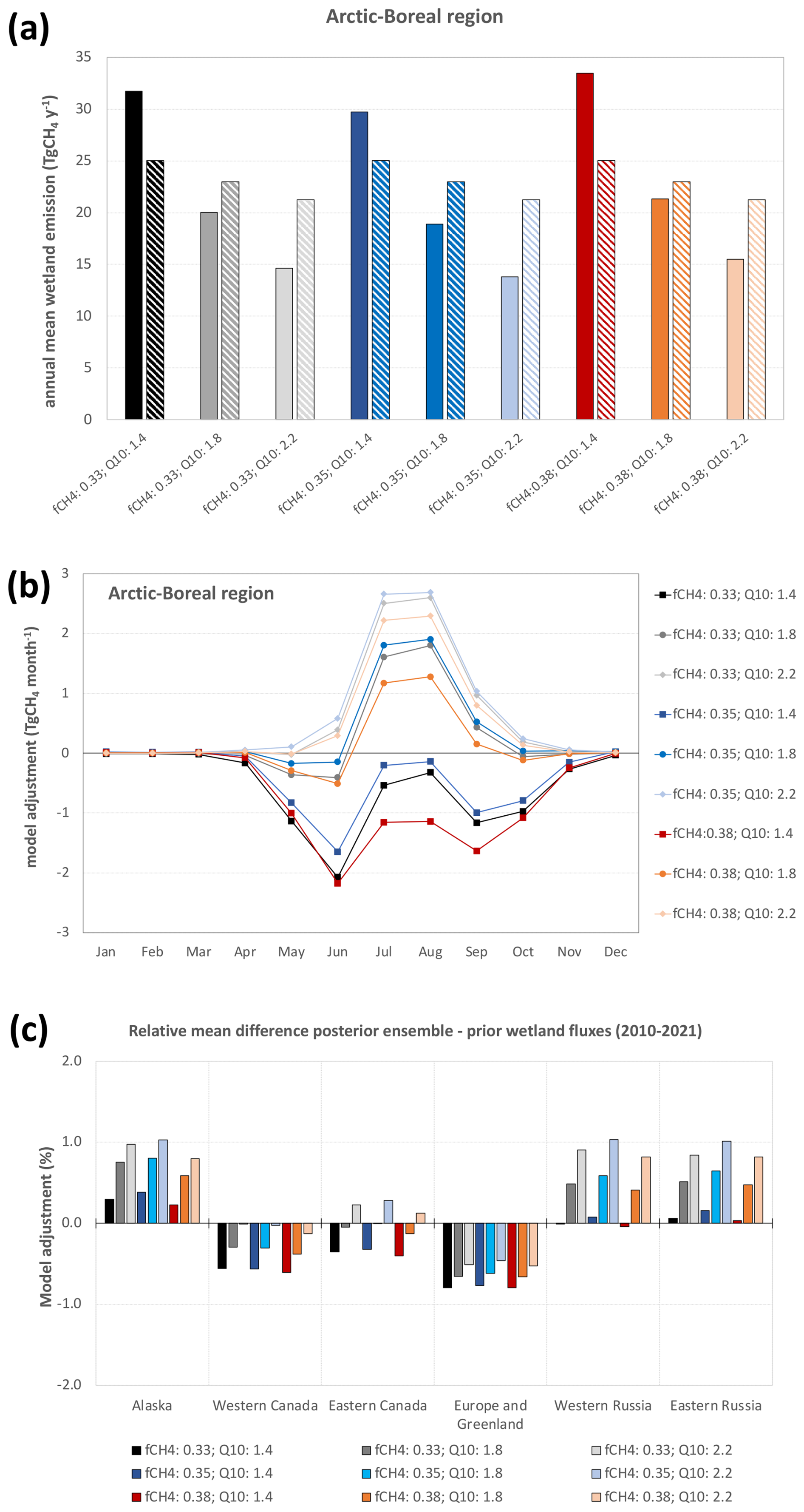
Figure 3 (a) Annual mean CH₄ emissions (prior: full color bars; posterior: dashed color bars) for the entire Arctic–Boreal region using all nine inversion scenarios with the different values of Q₁₀ parameter and baseline $f_{{\mathrm{CH}}_{\mathrm{4}}}$ fraction in JSBACH wetland emissions. (b) adjustment of prior fluxes at monthly timesteps for the same model configurations as used in (a). (c) relative annual mean model adjustment as percentage of prior (posterior ensemble minus prior flux) for each one of the sub-regions. Positive values indicate regions where prior estimates underestimated emissions compared with posterior estimates, while negative values represent areas where prior emissions overestimate CH₄ emissions compared with the posterior estimates.

Our posterior estimates of CH₄ emissions from wetlands are similar to previous Arctic–Boreal estimates. Using a process-oriented ecosystem model, Christensen et al. (1996) estimated a total CH₄ emissions from northern wetlands and tundra (>50° N) to be 20±13 Tg CH₄ yr⁻¹. Yuan et al. (2024) reported a mean annual emission of 20.3±0.9 Tg CH₄ yr⁻¹ from Boreal–Arctic wetland based on upscaled flux observations for the period 2002–2021. The Global Carbon Project estimated a mean annual wetland (including inland freshwaters) CH₄ emission for regions north of 60° N at 24 (9–53) Tg CH₄ yr⁻¹, while top-down approaches resulted in a lower estimate of 9 (7–17) Tg CH₄ yr⁻¹ for the same region (Saunois et al., 2025). Recently, Ying et al. (2025) estimated an annual mean CH₄ emissions from vegetated wetlands north of 45° N during 2016–2022 at 22.8±2.4 Tg CH₄ yr⁻¹, ranging from 15.7±1.8 to 51.6±2.2 Tg CH₄ yr⁻¹, depending on the wetland dataset used in the machine-learning-based upscaling approach. Although our posterior estimates are within the range of previous Arctic–Boreal estimates, direct comparisons are difficult because of differences in the study period, methodological approach, and inconsistent or unclear definitions of the spatial domain.

3.3 Seasonal variability in optimum CH₄ production Q₁₀ settings

Before analyzing regional differences in optimum CH₄ production Q₁₀ settings, we first focused on a clear seasonal pattern in the adjustments between prior and posterior CH₄ emissions, which showed a peak of changes occurring during summer. We therefore assessed whether the Q₁₀ value resulting in the minimum adjustment remained constant throughout the year or varied by season. At a pan-Arctic scale, seasonal variations were evident: estimates using CH₄ production Q₁₀ equaling 1.8 aligned better with atmospheric observations in spring and fall but substantially underestimated summer emissions (Fig. 3b). In contrast, estimates using a Q₁₀ of 1.4 best aligned with the atmospheric observation during summer, reducing the discrepancy between top-down and bottom-up estimates during the growing season, but strongly overestimating emissions in spring and fall (Fig. 3b). This pattern is primarily driven by wetlands in Russia. Bergman et al. (2000) found temporal variation in Q₁₀ at peatland sites, suggesting that factors such as the availability of easily degradable compounds (e.g., root exudates) and the activity of anaerobic microbial biomass influence CH₄ production rates alongside temperature.

3.4 Spatial patterns of best-fit model results based on posterior fluxes

CH₄ emissions exhibited spatial variability, and model adjustments were not uniform across the domain. This suggests that the optimal parameterization varies by region and seasons (as discussed in Sect. 3.3). In some areas, Q₁₀ values of 1.4 or 2.2 resulted in minimal adjustments (Fig. 3c), outperforming the model using a Q₁₀ equaling 1.8 that was shown to work best as an average setting across the entire domain. To better evaluate this variability and explore ways to reduce uncertainty in specific regions, we assessed the best parameterization fit with observations at the per grid-cell level (Fig. 4).

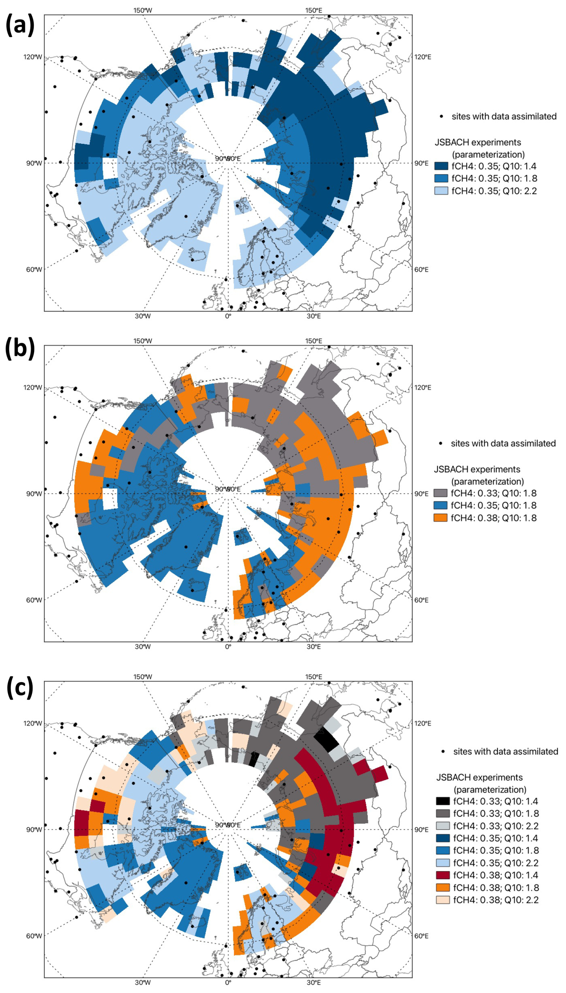
Figure 4 Map of the prior flux setting leading to minimum model adjustment (posterior ensemble minus prior fluxes) for the annual mean fluxes at each grid-cell for the Arctic–Boreal region varying the (a) CH₄ production Q₁₀ parameter only, (b) baseline $f_{{\mathrm{CH}}_{\mathrm{4}}}$ fraction only and (c) both Q₁₀ parameter and baseline $f_{{\mathrm{CH}}_{\mathrm{4}}}$ fraction. As mentioned in Sect. 3.2, the configuration with Q₁₀=1.8 and $f_{{\mathrm{CH}}_{\mathrm{4}}}=\mathrm{0.38}$ provides the best fit at the pan-Arctic scale. However, regional results show that this configuration does not minimize flux adjustments everywhere.

In our first analysis, we evaluated the spatial best fit model by keeping the baseline constant at a value of 0.35 and varying the CH₄ production Q₁₀ values (Fig. 4a). This spatial analysis showed that, in general, in regions with large wetland areas and high annual CH₄ emissions (for example the Western Siberian Lowlands, Figs. S1 and S2 in the Supplement) a Q₁₀ value of 1.4 resulted in the smallest model adjustment. As an increase in the Q₁₀ parameter decreases CH₄ production for temperatures below 295 K, a higher Q₁₀ value in these regions results in an underestimation of emissions. In contrast, regions such as Europe and northern Canada showed, in general, minimum model adjustments with a Q₁₀ value of 2.2, suggesting that lower Q₁₀ value would overestimate wetland CH₄ emissions in these regions. Interestingly, we observed adjustments with different signs in eastern Canada depending on the parameterization. For example, positive adjustments were associated with Q₁₀ value of 2.2, as the prior emissions were underestimated compared with the estimated flux inferred from atmospheric observations. Additionally, we analyzed the effect of varying baseline flux values while keeping Q₁₀ constant as 1.8, which showed that in high-emission areas, for example the Western Siberian Lowlands (Figs. S1 and S2), in general a larger baseline flux value led to the smallest model adjustments (Fig. 4b). When considering the model adjustment for all sensitivity tests (varying both CH₄ production Q₁₀ and baseline $f_{{\mathrm{CH}}_{\mathrm{4}}}$ fraction) as shown in Fig. 4c, we also found a consistent pattern that confirmed the above findings varying only single parameters: the combination of higher baseline fluxes and lower Q₁₀ value (Q₁₀=1.4) best captured CH₄ dynamics in CH₄ hotspots, as the Western Siberia Lowlands.

The wide range of reported incubation-based Q₁₀ values for CH₄ production in Arctic and northern wetlands depending on the site, substrate, and season, shows that the temperature sensitivity of CH₄ production varies considerably across environments (Bergman et al., 2000; Roy Chowdhury et al., 2015; Treat et al., 2015). This variability, which could be driven by factors such as vegetation type, organic matter quality, and microbial activity, emphasizes the necessity of models to account for spatial differences in process rates. For example, one synthesis study reported a mean Q₁₀ value of 1.18 for CH₄ production under Arctic soil conditions (Roy Chowdhury et al., 2015; Treat et al., 2015). Roy Chowdhury et al. (2015) used anoxic laboratory incubations of active layer and permafrost samples from the Barrow Environmental Observatory in Alaska and reported a range of Q₁₀ values from 1.8 to 22. Lupascu et al. (2012) reported that Q₁₀ values describing the CH₄ production response of peat to a 10 °C temperature change ranged from 1.9 to 3.5 in sedge sites and from 2.4 to 5.8 in Sphagnum mire sites, and suggested that using spatially variable CH₄ production Q₁₀ values could improve the accuracy of CH₄ flux modeling in northern wetlands. Furthermore, Bergman et al. (2000) found that the seasonal average Q₁₀ values ranged from approximately 4.6 to 9.2 depending on the plant community of the various peat types. Here, our intent is not to directly compare our results with reported incubation-based values, since our adjustments in the CH₄ production Q₁₀ refer to the Q₁₀ of the CH₄:CO₂ production ratio, as represented in the model, and could not directly be comparable with CH₄ production Q₁₀ from the literature review. In JSBACH, the Q₁₀ applied to CH₄ production controls the fraction of CH₄ generated, but the surface emission ratio may still be lower due to oxidation and transport pathways. Together, these examples highlight that CH₄ production is strongly temperature dependent, and that the degree of this dependency can differ across regions and time periods. However, most current models cannot fully capture the influence of these factors due to structural limitations or a lack of detailed input data that is both spatially and temporally resolved. Consequently, these environmental drivers are often oversimplified or overlooked. Adjusting the CH₄ production Q₁₀ values, as we do here, offers a useful initial approach, but it should not be seen as a long-term solution. Ideally, future model and data developments will enable CH₄ production Q₁₀ values to adjust dynamically in response to underlying biophysical conditions, such as shifts in vegetation or organic matter characteristics. This will allow models to operate with a more generalizable formulation that still captures observed heterogeneity. Recent studies have demonstrated the potential of methane data assimilation techniques to optimize process-model parameters using observational constraints (Bernard et al., 2025; Monteil et al., 2025); however, regional and seasonal optimization remains largely unexplored. While our model experiments identified a single CH₄ production Q₁₀ value that best agrees with observations at the pan-Arctic scale, they also showed that CH₄ emissions and model adjustments vary regionally. Some areas showed a substantial response to different Q₁₀ values, which further demonstrates that an approach using a single parameter value is not sufficient. This highlights the need for future data assimilation frameworks that allow for regional, and potentially seasonal, parameter optimization.

3.5 Limitations of Top-Down CH₄ estimates

Our analysis shows that atmospheric inverse modeling is a useful tool for evaluating and guiding process-model parameterizations when estimating wetland CH₄ emissions. However, it is important to note the limitations of the top-down approach, especially its relatively coarse spatial resolution. Global inversions usually operate at spatial scales larger than the process models, limiting their ability to resolve fine-scale heterogeneity, local emission hotspots, and small-scale processes. Consequently, grid-cell-level emission estimates represent aggregated signals and cannot fully capture localized variability.

Additionally, top-down estimates rely heavily on the spatial and temporal distribution of atmospheric observations assimilated into the model. Regions with sparce coverage, such as central and eastern Russia, can limit the ability to accurately identify emission sources and increase dependence on prior estimates. Furthermore, most surface observation sites at high latitudes only started providing measurements in the early 2010s. This limits the ability to assess multi-decadal changes in CH₄ emissions (Vogt et al., 2025).

At the grid-cell scale, assimilating only atmospheric CH₄ observations reflect the combined influence of all sources and sinks, making it difficult to distinguish overlapping source sectors. However, differences in the spatial patterns and seasonality of emissions can be constrained by atmospheric CH₄ observations in inversions that solve for different source categories (Saunois et al., 2025). Furthermore, errors in atmospheric transport model can propagate into emission estimates (Houweling et al., 2017; Locatelli et al., 2013; Schuh et al., 2019). Despite these limitations, our approach demonstrated a strong potential to help reduce the discrepancy between bottom-up and top-down estimates, therefore improving the accuracy of wetland CH₄ emission estimates.

4 Conclusions

Overall, our parameter sensitivity tests of bottom-up wetland emissions indicate that CH₄ production Q₁₀ has a stronger effect on emission variability than the baseline $f_{{\mathrm{CH}}_{\mathrm{4}}}$ fraction. Our bottom-up estimates showed that increasing CH₄ production Q₁₀ from 1.4 to 2.2 decreased the annual mean wetland CH₄ emission in the Arctic–Boreal region by half. In addition, our analysis shows that a single Q₁₀ value cannot capture the complexity of CH₄ emission dynamics across the Arctic–Boreal region. CH₄ production Q₁₀ values of 1.8 and 2.2 underestimate hotspot emissions, mainly during summer. In contrast, a Q₁₀ value of 1.4 overestimates emissions in regions with lower annual mean wetland emissions, such as e.g., Europe and northern Canada. Furthermore, a baseline $f_{{\mathrm{CH}}_{\mathrm{4}}}$ fraction value of 0.38 led to the smallest model adjustments in CH₄ hotspots. These findings emphasize the importance of selecting appropriate parameterizations to accurately represent wetland emissions, especially in regions with substantial CH₄ release. Future models should incorporate dynamic, data-driven adjustments to reflect underlying environmental controls more accurately. If a varying CH₄ production Q₁₀ value approach is not feasible for this region due to computational cost or model setup constraints, using a Q₁₀ value of 1.8 provides the more similar CH₄ emission estimates compared to the atmospheric data across the entire Arctic–Boreal region.

Our results demonstrate that, despite the inherent limitations of top-down approaches when it comes to resolving fine scale heterogeneity, combining atmospheric inversions and process-models provides an important tool for reconciling discrepancies between bottom-up and top-down estimates, thereby improving constraints on large-scale wetland methane emissions. Guidance by atmospheric inversion could therefore be instrumental to ensure the regional representativeness, and where applicable temporal variability, of process model parameter settings.