Carbon dioxide release driven by organic carbon in minerogenic salt marshes

Coastal wetlands play an important role in the global carbon cycle by sequestering carbon (referred to as “blue carbon”). At the same time, organic carbon (OC) in the subsurface is decomposed, releasing greenhouse gases (GHGs) such as carbon dioxide (CO₂) and methane (CH₄). To predict how this carbon balance in salt marshes will change under future climate scenarios (e.g., higher temperatures, sea level rise), it is essential to understand the controls on OC decomposition in these systems. Here, we investigated OC turnover and CO₂ release in a minerogenic salt marsh at the Wadden Sea, Germany. We first characterized the porewater and sediment of a pioneer marsh and adjoining intertidal flat to identify key biogeochemical processes. We then performed an in situ experiment by injecting two OC sources (labile (acetate)/complex (humic acid)) and subsequently monitored GHG release over four injection cycles along with subsurface geochemistry. Overall, we found that electron acceptors, primarily sulfate (SO${}_{\mathrm{4}}^{\mathrm{2}-}$), were present at all tested depths and no CH₄ was detected, suggesting that electron acceptor availability was unlikely to be the primary limiting factor on microbially mediated CO₂ release; the availability of OC (concentration and composition) may rather act as a limiting factor. Following the addition of labile OC, CO₂ release in the pioneer marsh increased by up to 47.4 ± 36.4 % compared to the control, with a generally similar trend in the intertidal flat. The CO₂ release from the complex OC treatment was similar to the control. The results of our work improve understanding of minerogenic salt marsh OC dynamics in temperate zones and enable better prediction of future changes.

1 Introduction

Vegetated coastal wetlands, located at the interface between land and the open sea, occur along all continental coastal zones except Antarctica and comprise mangroves, seagrass, and salt marshes (Nellemann et al., 2009; Pendleton et al., 2012; Tan et al., 2025). Salt marshes, including the seaward adjoining intertidal flats, sequester high amounts of carbon primarily in the sediment (Mcleod et al., 2011; Nellemann et al., 2009; de Vlas et al., 2013). Globally, around 60.4–70.0 Tg yr⁻¹ of carbon is buried in vegetated salt marshes (Duarte et al., 2005; Nellemann et al., 2009). The sequestration of carbon is disproportional in vegetated coastal areas, with around half of the total organic carbon in ocean sediment (often referred to as “blue carbon”) buried in these areas which only account for 0.2 % of the ocean surface (Duarte et al., 2013; Nellemann et al., 2009). As the rate of carbon input into the sediment exceeds its rate of decomposition (especially for allochthonous carbon), salt marshes are characterized by high carbon sequestration rates (Mueller et al., 2019; Temmink et al., 2022; Van de Broek et al., 2018). Simultaneously, salt marshes release greenhouse gases (GHGs) due to organic carbon (OC) decomposition: carbon dioxide (CO₂) at 0.02–0.24 Pg CO₂ yr⁻¹ (Pendleton et al., 2012) and methane (CH₄) at 0.142 ± 0.02 Mg carbon ha⁻¹ yr⁻¹ (Alongi, 2020). Therefore, understanding carbon turnover in coastal wetlands is crucial for predicting how these ecosystems will respond to climate change, such as temperature increase, sea level rise, and eutrophication of coastal waters. This is especially important given the annual 1 %–2 % loss of salt marshes due to land-use change and their vulnerability to climate impacts (Duarte et al., 2008).

In coastal wetlands, microbial respiration pathways couple OC as an electron donor with terminal electron acceptors (TEAs), especially oxygen (O₂), ferric iron (Fe(III)) and sulfate (SO${}_{\mathrm{4}}^{\mathrm{2}-}$) (Tan et al., 2025; Tobias and Neubauer, 2019). Oxygen, the thermodynamically most favourable TEA, exhibits fluctuating penetration depth into the sediment due to tides, bioturbation or root-mediated O₂ transport (de Beer et al., 2005; Huettel et al., 2014; Maricle and Lee, 2002). In deeper sediment layers, where anoxic conditions can dominate, microorganisms utilize Fe(III), from iron minerals, or SO${}_{\mathrm{4}}^{\mathrm{2}-}$, which infiltrates the sediment through inundation of seawater, as alternative TEAs (Jørgensen et al., 2019; Tobias and Neubauer, 2019). Upon full depletion of TEAs, OC is further decomposed to CH₄ (Schlesinger and Bernhardt, 2013b). Microbial decomposition of OC may be further influenced by its chemical composition. Chemically simpler e.g., short chain aliphatic OC may be substantially favoured for decomposition compared to complex OC, such as natural organic matter (Gunina and Kuzyakov, 2022; Lipczynska-Kochany, 2018; Schlesinger and Bernhardt, 2013a).

The primary controls on GHG release in salt marshes, as interfaces between land and open ocean, are not fully understood. Specifically, it is unclear whether OC turnover is primarily controlled by the availability of the electron acceptors – as observed in organogenic marshes and consistent with studies in terrestrial wetlands (Schlesinger and Bernhardt, 2013b) – or by the organic matter itself, as suggested for marine sediment in general (Arndt et al., 2013). Past studies on OC dynamics (including GHG release) in salt marshes have largely concentrated on the eastern coast of the US (Capooci et al., 2024; Kostka et al., 2002b; Lowe et al., 2000; Seyfferth et al., 2020), which is dominated by organogenic peat marshes. Organogenic marshes are generally low energy, microtidal wetlands, characterized by a high organic matter deposition via autochthonous pathways that results in high TOC contents (Logemann et al., 2025). For example, Lowe et al. (2000) and Kostka et al. (2002a) observed that OC oxidation was controlled by SO${}_{\mathrm{4}}^{\mathrm{2}-}$ and Fe(III) reduction in salt marshes in Georgia, USA. Further, CH₄ fluxes were detected in salt marshes in Delaware, suggesting a co-occurrence of methanogenesis and SO${}_{\mathrm{4}}^{\mathrm{2}-}$ reduction (Capooci et al., 2024; Seyfferth et al., 2020). European salt marshes, in contrast, are primarily minerogenic, i.e., contain high fractions of mineral sediment due to high sedimentation rates, resulting in comparably lower TOC content (Nolte et al., 2013). Studies conducted in European salt marshes have focused on the TEA turnover (e.g., SO${}_{\mathrm{4}}^{\mathrm{2}-}$ respiration rates) and not GHG emissions (de Beer et al., 2005; Bosselmann et al., 2003; van Erk et al., 2023). These studies showed that O₂ penetrates down the sediment, Fe(III) is available and SO${}_{\mathrm{4}}^{\mathrm{2}-}$ reduction occurs. Hence, these studies have provided indirect links between belowground biogeochemistry, especially in the context of available TEA, and the release of GHGs in minerogenic salt marshes; however, a direct investigation of the determining factor(s) of OC degradation from these ecosystems is missing. By understanding the controls on GHG release, we can better predict how climate impacts such as higher temperatures and sea level rise will affect OC turnover and thereby GHG release in minerogenic salt marshes.

To investigate the in situ carbon dynamics in minerogenic salt marshes, we chose a representative field site at the Wadden Sea coast. Our goals were (i) to identify the key microbial processes (O₂, Fe(III) and/or SO${}_{\mathrm{4}}^{\mathrm{2}-}$ reduction) that control the release of OC as CO₂ and/or CH₄, and (ii) to determine the role of OC (concentration and composition) in the release of GHGs. To this end, we first characterised the primary geochemical parameters from a minerogenic pioneer marsh and intertidal flat at the German Wadden Sea. Building on those results, we conducted an in situ manipulation experiment investigating the impact of two contrasting OC sources (acetate, humic acid) on GHG emissions. We hypothesized that (i) the high energy and sediment inputs in minerogenic salt marshes result in low TOC supply and high TEA availability. (ii) We further hypothesize that this leads to the likely limitation of electron donor and not acceptor on OC decomposition and (iii) the composition of OC plays a more important role than the concentration in CO₂ release from a minerogenic salt marsh. These hypotheses were tested in two successional zones of a salt marsh, a pioneer marsh with sparse pioneer vegetation and a non-vegetated intertidal flat.

2 Materials and Methods

2.1 Study site

This study was conducted at the Altfelder Koog by Friedrichskoog (54°01^′02.4^′′ N, 08°51^′17.09^′′ E), an area that consists of a salt marsh with different successional zones in the Wadden Sea National Park (Schleswig-Holstein) in northern Germany at the mouth of the Elbe estuary (Fig. 1a). The Wadden Sea is a UNESCO World Heritage Site and the largest continuous salt marsh (including tidal flats) in Europe (Common Wadden Sea Secretariat, 2017). The tidal range at the study area is 3.59 m, defined as the difference between mean height of high water and approximately the lowest astronomical tide. The mean high tide is 1.56 m higher than the mean sea level (BSH, 2025).

At the Wadden Sea, different successional zones of salt marshes are developing as a result of the ongoing process of sediment transportation by waves and tides (Esselink et al., 2017; de Vlas et al., 2013). The two successional zones which are of interest in our study are the pioneer marsh and the intertidal flat (Fig. 1a). Pioneer species such as Salicornia spp. and Spartina anglica occur in the pioneer marsh, promoting further sediment trapping (Esselink et al., 2017; de Vlas et al., 2013). The intertidal flat (seaward of a pioneer marsh) is an area with no plants to buffer incoming waves and is therefore subject to a strong tidal influence (Esselink et al., 2017). In general, both the pioneer marsh and intertidal flat are inundated daily during high tide, with the pioneer marsh experiencing less and shorter inundation (< 3 h fully inundated) compared to the intertidal flat (> 3 h fully inundated) (de Vlas et al., 2013). During a spring tide, which occurs twice a month, the magnitude of high and low tide is amplified leading to stronger exposure of the pioneer marsh to tides (Gao, 2019; Kvale, 2006).

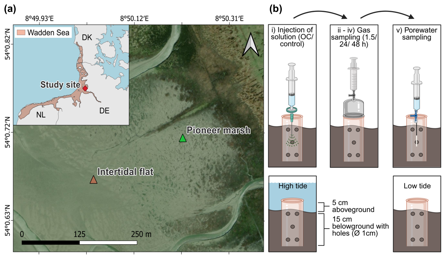
Figure 1 Study site at the Wadden Sea including the successional zones of a salt marsh and a schematic representation of the in situ experimental design. (a) Wadden Sea, in light red in the inset with a red marker indicating our study site in northern Germany (Friedrichskoog, Elbe estuary). Gradient of salt marsh succession zones, beginning with the intertidal flat, followed by the pioneer marsh and more developed successional zones extending further inland. Map information: Reference system WGS 1984, UTM 32N, Esri | Powered by Esri. (b) Experimental design: experimental procedure (top) and cylinder setup in sediment (below). Each sampling plot consisted of a 20 cm long cylinder (diameter 16 cm), drilled with 1 cm diameter holes along the length of the cylinder. The cylinder was inserted 15 cm deep in the sediment to define the injection area. The top 5 cm was used to mount a gas chamber during gas sampling. The cylinder stayed in the sediment over the course of the experiment including high and low tide. Numbers (i)–(v) indicate the experimental procedure: (i) injection of solution (acetate or humic acid, only NaCl for control), (ii) 1.5 h after injection, the first gas measurement was done, (iii) followed by the second gas measurement after 24 h of injection, and (iv) the final gas measurement after 48 h of injection, followed by the final step of (v) porewater sampling. Each treatment (acetate, humic acid) and the control consisted of spatial triplicates.

2.2 Porewater and sediment sampling for general geochemistry

In August 2022 and 2023, sediment cores were collected from the pioneer marsh and intertidal flat to analyse the general geochemistry of the sediment and porewater. The sampling was performed during low tide. Push cores were collected using core liners (UWITEC, polyvinyl chloride PVC) with an inner diameter of 8.6 cm (outer diameter 9 cm) and a length of 60 cm. To minimize compression, we used open push cores and only capped them when the core liner was fully in the sediment. Furthermore, the inside wall of the cores was plain and clean to smoothly insert the core liner in the sediment. To further minimize disturbance, the sampled cores were immediately closed, vertically transported, and stored in the dark. At depth intervals of 5 cm, porewater samples (Rhizon sampler CSS, 0.12–0.18 µm pore size, Rhizosphere Research, Netherlands) and sediment samples (using a cut-off syringe) were taken through pre-drilled holes which had been covered with isolation tape during coring. We made sure to not take sediment or porewater samples at the edges but rather from the middle of the cores, where the sediment is likely undisturbed. Porewater samples were analysed for dissolved organic carbon (DOC), iron speciation, SO${}_{\mathrm{4}}^{\mathrm{2}-}$, and dissolved CH₄, and sediment samples for total organic carbon (TOC). Detailed method for dissolved CH₄ sampling is given in Supplement Sect. S1.1.

We collected further sediment cores for fine scale O₂ profiles. For this, sediment push cores (inner diameter 2.5 cm, length 10 cm) were collected and immediately sealed. Shortly after sampling, O₂ profiles were taken with a depth resolution of 500 µm using Clark-type O₂ microsensors (Unisense, Denmark) with a 100 µm tip, following Revsbech (1989). Before measurement, a two-point calibration was done using air-saturated seawater and 0.1 M sodium ascorbate in 0.1 M NaOH solution. Profiles were recorded with the Unisense software SensorTrace Suite (version 2.8.200.21688, Unisense, Denmark).

2.3 Physicochemical characteristics of the sediment

For a general physicochemical characterization, bulk sediment was collected from a depth up to 15–20 cm in sterile sample bags with puncture proof tabs (Nasco, Whirl-pak, USA), and stored at 4 °C in the dark. Stones and macrofauna were removed prior to further analysis. We determined grain density, bulk porosity, moisture content, and particle size (details in Supplement Sect. S1.2).

2.4 In situ experiment: Enhanced organic carbon input

2.4.1 In situ experiment design

An in situ OC addition experiment was conducted in August and September 2023 to test the response of pioneer marsh and intertidal flat systems to elevated inputs of OC with different compositions. We choose acetate, a chemically simple organic compound that has been detected at other salt marshes (Hyun et al., 2007; Kostka et al., 2002a) and at a site nearby (Llobet-Brossa et al., 2002), and humic acid (in the form of Pahokee Peat humic acid), a more complex OC source, as a proxy for natural organic matter. The two OC sources were chosen, knowing their thermodynamical difference from previous studies (Gunina and Kuzyakov, 2022), to present a fermentation product (acetate) and a proxy for terrestrial organic matter (in addition to the difference with respect to complexity). Studying both labile and complex OC additions is ecologically relevant as salt marshes receive OC from multiple sources (Howard et al., 2023; Temmink et al., 2022). Eutrophication of coastal waters and/or root exudates can supply readily degradable OC to salt marshes, while increased organic matter load in rivers can deliver more complex OC compounds to salt marshes. The applied OC compounds in our study, therefore, represent environmental scenarios and allows us to investigate how these OC sources influence GHG release under realistic conditions. The injection solutions were prepared in the laboratory prior to use in the field. Solutions of 1 g OC L⁻¹ were prepared with either acetate or humic acid as a carbon source. For the preparation of the solutions, sodium acetate or Pahokee Peat humic acid (obtained from the International Humic Substances Society (IHSS), Table S1) were dissolved in deionized water (Barnstead MQ system, Thermo Fisher Scientific, Germany), the pH was adjusted to 7.07–7.81 and NaCl was added (20 g L⁻¹). The solution for the control only contained NaCl. Additionally, 25 mM bromide (Br⁻) (in the form of NaBr) was added into the carbon and control solutions as an inert tracer in the field. All solutions were purged with nitrogen and stored at 4 °C in the dark until used in the field. Details of the preparation process are provided in Supplement Sect. S1.3.

The in situ experiment was performed in the pioneer marsh (54°00^′43.14^′′ N, 08°50^′12.9^′′ E) and intertidal flat (54°00^′40.45^′′ N, 08°50^′02.27^′′ E) (Fig. 1a), with the same setup in both zones. The assigned plots in the field were selected as visually similar triplicates (spatial triplicates), at a distance of ∼ 5 m between plots of the same treatment and ∼ 10 m between different treatments and the control plots. In the pioneer marsh, plots were placed outside of vegetated areas, i.e., the actual plot area of injection and sampling were free of vegetation although vegetation was present in the vicinity (Fig. S1a, b). For the intertidal flat, no vegetation was present, neither in the surroundings nor inside of the plots (Fig. S1c, d). Each plot consisted of a 16 cm diameter PVC cylinder with both ends open which was pushed 15 cm deep into the sediment (Fig. 1b). Holes (diameter 1 cm) were drilled in the cylinder wall to allow underground water movement. A porewater sampler (Rhizon sampler CSS, 0.12–0.18 µm pore size, Rhizosphere Research, Netherlands) was inserted in the middle of each plot at a depth of 5–10 cm and remained in the sediment over the duration of the experiment. The cylinder reached 5 cm out of the sediment, allowing a gas flux chamber to be mounted gastight for gas measurements. During the experiment, the cylinder stayed in the field. To decrease the influence of disturbances due to the setup of the experiment, we waited at least three days between setting up and the first measurements. Apart from the incubation time for gas sampling, the sediment within the cylinder was exposed to the atmosphere (low tide) or covered with seawater (high tide) (Fig. 1b).

The experiment was conducted similarly in both zones, the pioneer marsh and intertidal flat, using spatial triplicates and comprising four injection cycles (Fig. 1b). One injection cycle consisted of (i) the injection of the anoxic sterile solution (OC or control solution), followed by (ii) the first gas sampling 1.5 h after the injection. Gas sampling was repeated (iii) 24 h after the injection and (iv) 48 h after the injection. After the 48 h gas sampling, (v) porewater was collected. Injection of the solutions and sampling was done during low tide. The solution for the different treatments was slowly injected in step (i) with a bent needle at a depth of approximately 5–10 cm in the middle of each plot into the sediment. The injected solution was filtered (PES filter, pore size 0.22 µm, pre-rinsed with double deionized water) during injection to ensure that the solutions were sterile.

In each injection cycle, the native OC was increased by 12.0 mg C L⁻¹ in the pioneer marsh and 12.6 mg C L⁻¹ in the intertidal flat, assuming an even distribution across the experimental cylinder (calculation in Supplement Sect. S1.4). After one cycle was completed, the system had three days to recover before the next injection. At the end of the four injection cycles, sediment samples were collected (details below). The applied approach allowed us to assess short-term OC process response in minerogenic salt marshes, rather than long-term responses.

2.4.2 In situ experiment sampling

Gas sampling

Gas sampling was conducted using an opaque, static, non-flow gas chamber made of polypropylene (chamber volume 3000 cm²). The gas chamber was placed on the cylinder and gas samples were collected at 20 min intervals over an incubation period of 1 h using a 50 mL gastight syringe with a three-way valve. For sampling, the chamber gas was gently mixed by pumping the syringe plunger three times before withdrawing 35 mL gas. The first 5 mL were used to flush the attached needle, and the rest was transferred immediately into a pre-evacuated 12 mL Exetainer^® vial (Labco, UK). The samples were measured with a Greenhouse GC equipped with two Pulsed Discharge Detector (PDD) (ThermoFisher Scientific TRACE™ 1310 GC-Analyzer, USA – custom designed by S+H-Analytik) and two column structure (first structure 30 m long, 0.53 mm ID TGBondQ column, second structure 30 m long, 0.53 mm ID Molsieve column (for CH₄) and 30 m long 0.32 mm ID TGBondQ+ column (for CO₂, N₂O)). Calculation for the gas fluxes and cumulative CO₂ emissions are given in Supplement Sect. S1.5.

Porewater sampling

Porewater samples were collected via the pre-installed porewater sampler. The pH (Mettler Toledo SevenGo, Germany) and salinity (refractometer) were measured in the field. The collected porewater was fixed for DOC (acidification with 2 M HCl), iron speciation (acidification with 1 M HCl), and total sulfide (S(II)_tot) (alkalinization with zinc acetate). Dissolved inorganic carbon (DIC) samples were transferred into vials without headspace immediately after sampling and capped. The remaining porewater was anoxically stored in nitrogen flushed bottles in the dark at 4 °C for Br⁻, SO${}_{\mathrm{4}}^{\mathrm{2}-}$ and chloride (Cl⁻) measurements.

Sediment sampling

At the end of the experiment, sediment samples were collected for geochemical analysis (TOC, solid iron speciation, sulfide species) and microbial analysis. For this, push cores (inner diameter of 2.5 cm, and a length 10 cm) were taken from the middle of each plot at the same positions as the porewater samples and immediately frozen until further analysis. Sediment samples for the molecular biology analysis were stored at −80 °C upon bringing them back to the laboratory.

2.5 Geochemical analysis

2.5.1 Porewater analysis

DOC (as non-purgeable OC) and DIC (as the difference of total carbon and OC) was determined by a TOC analyser (multi N/C 2100S, Analytik Jena GmbH, Germany). To analyse the iron speciation in the porewater, the ferrozine assay (Stookey, 1970) was used. The S(II)_tot was quantified by the Cline assay (Cline, 1969). Sulfate, Br⁻, and Cl⁻ were analysed by an ion chromatograph (Metrohm 930 Compact IC Flex, Switzerland).

2.5.2 Sediment analysis

For all sediment analyses, sampled cores were thawed in an anoxic glovebox to prevent oxidation (UNIlab plus Glovebox, MBRAUN, Germany), sliced in two depths (0–5 and 5–10 cm), and each depth fraction was homogenized by hand.

Iron extraction

To target the poorly and higher crystalline iron phases in the sediment samples, parallel iron extractions were performed under anoxic conditions, adapted from Moeslundi et al. (1994) and Lueder et al. (2020). From each depth (0–5 and 5–10 cm) ∼ 0.2 g wet sediment sample (in triplicates) were added into an Eppendorf tube. To extract poorly crystalline iron minerals, we used an extraction with anoxic 0.5 M HCl (Heron et al., 1994). We expect that poorly crystalline iron (oxyhydr)oxides as well as ferrous iron (Fe(II)) phases such as carbonates and sulfides (e.g., FeCO₃ or FeS) would be extracted by this acidification. One mL of anoxic 0.5 M HCl was added to the sediment, vortexed, and incubated for 2 h in the dark at room temperature in the glovebox. For the extraction of iron minerals of higher crystallinity, targeting more crystalline Fe(II) (except pyrite) and Fe(III) phases (Cornwell and Morse, 1987; Heron et al., 1994), 1 mL of anoxic 6 M HCl was added to the sediment, and the sediment was vortexed and vertically rotated for 24 h under anoxic conditions at room temperature (30 rpm, dark). For both HCl extractions, the samples were then centrifuged (5 min, 13400 rpm), the supernatant was diluted with 1 M HCl, and iron speciation and concentration of the supernatant was determined using the ferrozine assay (Stookey, 1970). Total iron and Fe(II) concentrations of the supernatant were measured directly, and Fe(III) was determined by subtracting Fe(II) from total iron. To obtain the higher crystalline fraction separately, the poorly crystalline fraction (0.5 M HCl extract) was subtracted from the 6 M HCl fraction. We acknowledge that the weaker acid extraction extracted Fe(II) from carbonates and sulfides in addition to iron (oxyhydro)oxides. We therefore used this approach to determine the crystallinity of iron minerals and call it poorly (extracted by 0.5 M HCl) and higher (extracted by 6 M HCl) crystalline iron minerals (and not (oxyhydr)oxides).

Acid volatile sulfide

To determine the mass of acid volatile sulfide (AVS) in the sediment similar to Burton et al. (2007), ∼ 2 g of wet sediment was weighed in centrifuge tube in a glovebox. A smaller tube filled with anoxic 1 M zinc acetate + anoxic 2 M NaOH ($v/v$ 15:85) was placed into the sediment-filled centrifuge tube. To the sediment, 10 mL anoxic 6 M HCl + 2 mL anoxic 1 M L-ascorbic acid was added and immediately closed. The double tubes were placed in an ultrasonic bath for 30 s, followed by horizontal shaking overnight (150 rpm). The sulfide released from the sediment was captured in the zinc acetate solution and was analysed according to Cline (1969).

Total organic carbon

To quantify sediment TOC, samples collected in 2023 were dried under anoxic conditions, while those from 2022 were dried under oxic conditions at room temperature until constant weight was reached. Sediments from both years were milled and analysed by a TOC analyser (SoliTOC Cube Elementar, Germany).

2.6 Molecular biology analysis

The co-extraction of DNA and RNA was performed according to Lueders et al. (2004). Quantitative polymerase chain reaction (qPCR) for DNA and complementary DNA (cDNA) was done to quantify total bacterial 16S rRNA gene copies using the primer 341F and 797R. Functional genes were also targeted: Geobacter spp. (involved in Fe(III) reduction) using the primer Geo577F and Geo822R, and dsrA (involved in SO${}_{\mathrm{4}}^{\mathrm{2}-}$ reduction) using the primer DSR_1F and DSR_1R. Quantitative polymerase chain reaction was done using SsOAdvanced SYBR Green Supermix (Bio-Rad) on the C1000 Touche Thermal Cycler (CFX96™ Real-Time System, Bio-Rad, Germany). Data analysis was performed by the software Bio-Rad CFX Maestro 1.1 (version 4.1.2433.1219). Further details are given in Supplement Sect. S1.6 and Table S2.

2.7 Statistical analysis

For statistical analysis RStudio (R version R-4.4.3) was used (R Core Team, 2025). The significance level for all tests was set at p < 0.05. Normal distribution of the data and homogeneity of variances were tested by Shapiro-Wilk test and Levene test, respectively. Correlations between parameters was tested with the relevant tests (Pearson's correlation test or Spearman's rank correlation test depending on the normality of the data). Statistical differences between two groups were tested with a t-test and for more than two groups with a one-way Analysis of Variance (ANOVA) or Kruskal-Wallis rank sum test. For differences in the CO₂ release, a linear mixed model was applied. More details on the chosen tests and model are given in Supplement Sect. S1.7. We reported the p-value in the text; further relevant statistical test results and parameters are shown in the corresponding sections in the SI. The variability of the geochemistry analysis is represented by the standard deviation of triplicates/duplicates. For the in situ experiment, the variability is reflected in the standard error of triplicates. For duplicate analyses, variability reflects the range of the two samples.

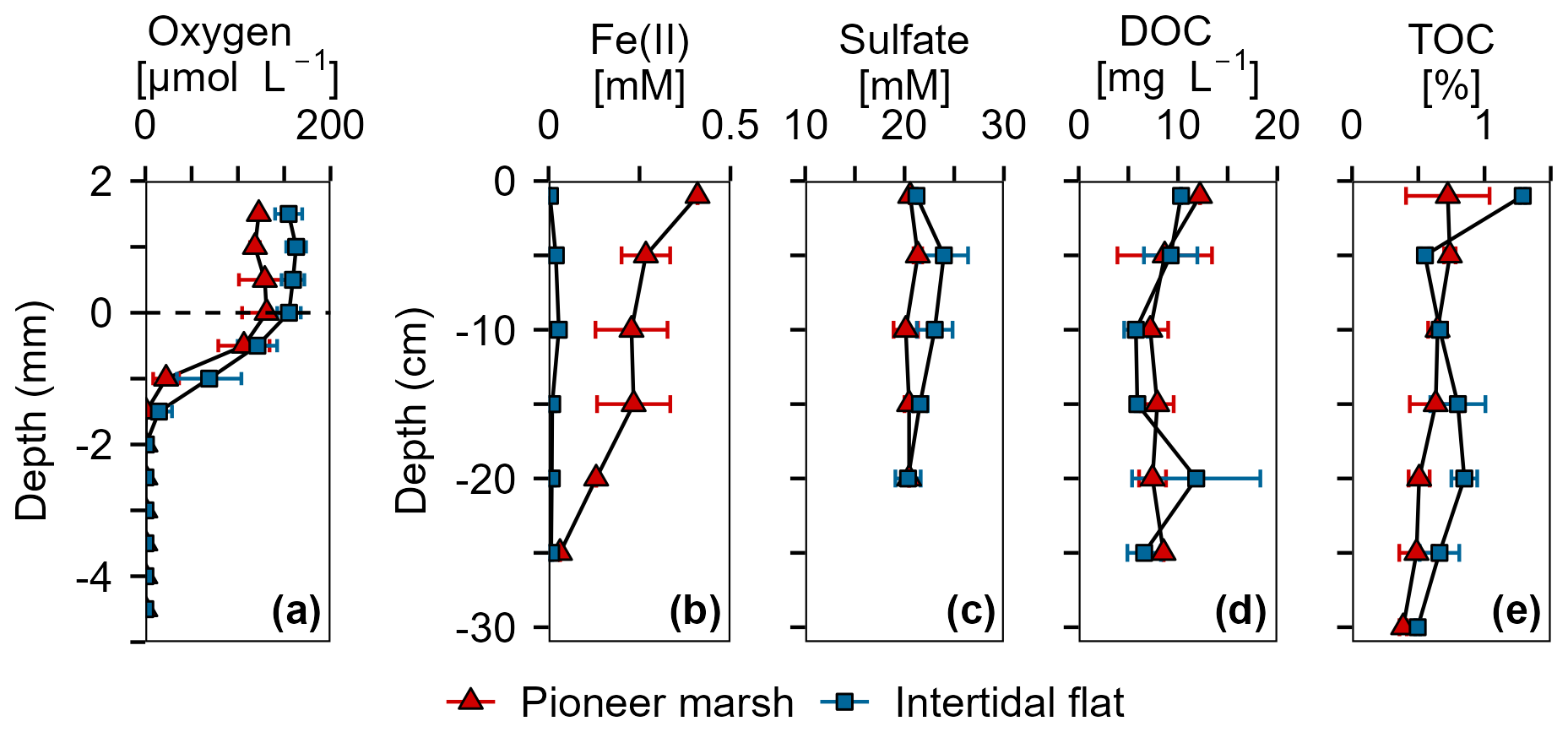
Figure 2 Overview of porewater and sediment biogeochemistry in terms of electron acceptors (O₂, Fe(III), SO${}_{\mathrm{4}}^{\mathrm{2}-}$) and electron donor (DOC, TOC) from in situ push cores in the pioneer marsh (red triangles) and intertidal flat (blue squares). (a) Oxygen concentration profiles measured in intact cores using microsensors. Note that these cores were collected in 2022, separate from the push cores used for analysis shown in (b)–(e). Two cores were collected from each zone and two to four profiles were taken from each core, shortly (within hours) after sampling. (b) Ferrous iron in the porewater, as an indicator of Fe(III) reduction. (c) Sulfate concentrations in the porewater. (d) Dissolved organic carbon in the porewater. (e) Total organic carbon in the sediment. For (b)–(d), push cores were taken in triplicates in both zones to a depth of 25 cm in 2023. Duplicate push cores for (e) the TOC were sampled in 2022. For all sub-figures, markers denote mean ± standard deviation (due to limited sample mass, some depth values only show mean and the range of two samples, or only a single value). All cores were sampled during low tide.

3 Results

3.1 Geochemistry at the study site

Porewater and solid phase measurements from the push and microsensor cores analysis show availability of electron acceptors (O₂, Fe(III), and SO${}_{\mathrm{4}}^{\mathrm{2}-}$) over depth in both the pioneer marsh and intertidal flat (Fig. 2). In the pioneer marsh, O₂ decreased from 131.02 ± 26.49 µmol L⁻¹ at the sediment-water interface to 0.18 ± 0.12 µmol L⁻¹ over 2 mm and was depleted beyond this depth. We observed a similar trend for the intertidal flat, with 155.17 ± 12.71 µmol L⁻¹ at the sediment-water interface, and a decrease to 0.62 ± 1.10 µmol L⁻¹ at 2 mm depth before it was fully depleted (Fig. 2a). Aqueous Fe(II) (as an indicator of Fe(III) reduction) showed a decreasing trend in both zones, with higher concentration in the pioneer marsh of 267.49 ± 66.77 µM at 5 cm depth and 31.41 µM at 25 cm, and 19.93 ± 16.15 µM at 5 cm decreasing to 7.20 ± 2.89 µM at 25 cm in the intertidal flat (Fig. 2b). Sulfate was detected in the porewater at all sampled depths (1.5 to 20 cm) in both zones (Fig. 2c). In the pioneer marsh, it ranged in the upper 20 cm from a minimum of 20.12 ± 1.23 mM to a maximum of 21.34 ± 0.43 mM and in the intertidal flat from 20.35 ± 1.27 to 23.95 ± 2.44 mM. We observed a slight decrease in SO${}_{\mathrm{4}}^{\mathrm{2}-}$ concentration over depth which was more pronounced in the intertidal flat. This is further supported by the ratio of sulfate:chloride (Fig. S2a). The ratio remained constant in the pioneer marsh, while a slight decrease was measured in the intertidal flat. We also measured SO${}_{\mathrm{4}}^{\mathrm{2}-}$ at lower depths (up to 50 cm) in cores taken in 2022 and observed similar SO${}_{\mathrm{4}}^{\mathrm{2}-}$ concentrations (Fig. S2b). To complement the porewater Fe(II), we measured the 0.5 M HCl extractable Fe(III) from the bulk sediment from a depth up to 15–20 cm: 1.30 ± 1.08 µmol Fe(III) g⁻¹ dry sediment in the pioneer marsh and 1.00 ± 0.51 µmol Fe(III) g⁻¹ dry sediment in the intertidal flat. The resulting Fe(II) to total iron ratio was 0.98 ± 0.02 and 0.98 ± 0.01 respectively.

Organic carbon as the likely electron donor was measured in the porewater as non-purgeable organic carbon and in the sediment as TOC. The DOC and TOC decreased slightly over depth (Fig. 2d, e) in both zones. In the pioneer marsh, the DOC was 12.21 mg C L⁻¹ at the top (1 cm deep) and decreased over depth to 8.55 mg C L⁻¹ at 25 cm. For the intertidal flat, the DOC at the top (1 cm deep) was 10.31 mg C L⁻¹ and decreased to 6.60 ± 1.69 mg C L⁻¹ at 25 cm. The TOC decreased from 0.7 ± 0.3 % at the top to 0.5 ± 0.1 % at a depth of 25 cm in the pioneer marsh and from 1.3 % to 0.7 ± 0.2 % in the intertidal flat (Fig. 2e). Concentrations at lower depths are shown in Supplement Fig. S2c, and are in a similar range. In both the pioneer marsh and intertidal flat, no CH₄ release, neither as fluxes or in the porewater up to a depth of 50 cm, was detected (detection limit: 0.28 and 0.53 ppm respectively; Table S3).

Particle size analysis indicated that sediment from the pioneer marsh was dominated by fine particles, whereas the intertidal flat sediment was coarser. In the sediment of the pioneer marsh, we determined 41.7 ± 9.1 % sand, 38.7 ± 2.5 % silt, and 19.7 ± 8.1 % clay. For the sediment of the intertidal flat, a higher sand fraction (61.5 ± 0.5 %), less silt (29.0 ± 5.0 %), and notably lower clay content (9.5 ± 5.5 %) was measured. For more details on the size fractions, see Supplement Table S4.

3.2 In situ organic carbon manipulation experiment

3.2.1 Distribution of bromide tracer and dissolved organic carbon in the sediment

Bromide was used in the in situ experiment as an inert tracer to test the washing out of the injection solution from the experimental plot over the sampling time of one injection cycle (48 h). The native Br⁻ concentration was 0.66 ± 0.02 mM in the pioneer marsh and 0.63 ± 0.01 mM in the intertidal flat. Assuming an equal distribution of the injected solution in the experimental cylinder, we expected the Br⁻ concentration to increase by 0.30 mM to a final concentration of 0.99 mM in the plots of the pioneer marsh and by 0.32 mM to a final concentration of 0.97 mM for the plots in the intertidal flat (calculations in Supplement Sect. S1.4 – expected Br⁻ concentration). Throughout a test injection cycle with the same sampling intervals as the experimental injection cycles, the Br⁻ concentration remained above the background level with a gradual decrease over time in both zones (Fig. S3a, b). Overall, after 48 h (one injection cycle), Br⁻ levels in the porewater remained elevated in each cycle for both zones. In the pioneer marsh, an average of 77.5 ± 5.9 % of the expected level of Br⁻ remained in the porewater of the experimental cylinder. The intertidal flat had a slightly lower average residual fraction of 72.1 ± 4.4 % of the expected Br⁻ level across all injection cycles (Fig. 3). Here, residual fraction is defined as the ratio between the Br⁻ concentration measured in the porewater 48 h post injection and the expected total Br⁻ concentration in an experimental cylinder (Eq. 1); details in Sect. S1.4). The expected total Br⁻ concentration includes both the native Br⁻ and the added Br⁻ during the experiment (expected Br⁻) after accounting for dilution in the sediment. Details on the calculation of the Br⁻ residual fraction are provided in Supplement Sect. S1.4.

$$\begin{array}{}\text{(1)}& {\displaystyle \frac{{\mathrm{Br}}_{\text{concentration at the end of an injection cycle}}^{-}}{{\mathrm{Br}}_{\mathrm{expected}}^{-}}}=\text{residual fraction}\end{array}$$

The residual fraction of DOC is defined in the same way as for Br⁻, representing the proportion of measured DOC after 48 h to the expected DOC (native DOC + added acetate/humic acid) and was calculated analogously to Br⁻, with DOC concentrations used instead (Eq. 1) and Sect. S1.4. Comparing the average residual fraction of DOC and Br⁻ (Fig. 3) across all injection cycles, the DOC fraction was significantly lower in both the pioneer marsh and intertidal flat (Br⁻ vs. acetate and Br⁻ vs. humic acid) (p≤0.001, Table S5). In the pioneer marsh, 40.0 ± 1.2 % of the injected DOC in the acetate treatment remained, on average across all injection cycles, while the corresponding value for the humic acid treatment was 52.9 ± 4.5 %. In the intertidal flat, relatively less carbon remained, with a smaller difference between the carbon sources. Here, the mean residual fraction was 38.2 ± 4.8 % for the acetate treatment and 37.3 ± 3.6 % for the humic acid treatment.

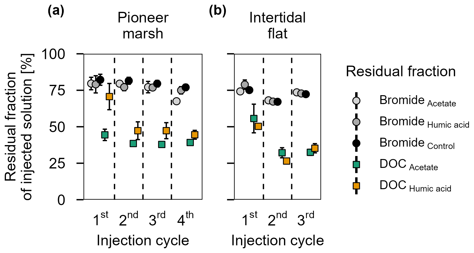
Figure 3 Residual fraction of injected solutions (Br⁻ and DOC) in percentage after 48 h for treatments (acetate, humic acid) and control plots in the (a) pioneer zone (over four injection cycles) and (b) intertidal flat (over three injection cycles). Coloured squares show the residual fraction of injected DOC (acetate in green and humic acid in orange). The grey shaded circles represent the residual of Br⁻ from the different treatments and the control. The values were calculated based on the ratio between the measured DOC or Br⁻ concentration (porewater concentration 48 h post injection) and the expected DOC or Br⁻ concentration (native + added). Markers represent the mean of the triplicates, with error bars indicating the corresponding standard error for treatments and control in both zones for DOC and Br⁻ across all injection cycles.

3.2.2 Effect of organic carbon input in the pioneer marsh

Carbon dioxide release

Figure 4 presents the CO₂ release for each injection cycle with the individual CO₂ fluxes 1.5, 24, and 48 h post injection (Fig. 4a) and the cumulative CO₂ emissions (Fig. 4b) in the pioneer marsh. For all four injection cycles, the CO₂ fluxes of the acetate treated plots exceeded the CO₂ fluxes of the humic acid and control plots (Fig. 4a). For the first injection cycle, the acetate treatment was significantly higher compared to the humic acid treatment (p<0.05, Table S6) and slightly above the threshold for statistical significance (p=0.08, Table S6) compared to the control. In the following injection cycle, the CO₂ fluxes of the acetate treatment were also higher compared to the humic acid and control plots but not significantly (p > 0.05). Hence, the acetate treated plot consistently exhibited the highest fluxes. The difference between the humic acid and control plots was statistically negligible (p > 0.05). Similarly, the cumulative CO₂ emissions from the acetate treated plots were the highest while the emissions from the humic acid and control plots were in a similar range for all four injection cycles (Fig. 4b). The CO₂ emitted from the acetate treated plots was up to 83.2 ± 53.7 % higher than for the humic acid treated plots. Similarly, the emissions of the acetate plots were up to 47.4 ± 36.4 % higher relative to the control plots. No statistical differences were measured between the cumulative CO₂ emission of the acetate treated plots and the control or humic acid treatment. Overall, these differences were smaller than those seen at individual CO₂ fluxes at specific time points (Fig. 4a), likely due to high variability in fluxes that resulted in variable cumulative CO₂ emissions. In all treatments and the control, no CH₄ as a flux was detected (lower than detection limit (0.28 ppm; Table S3).

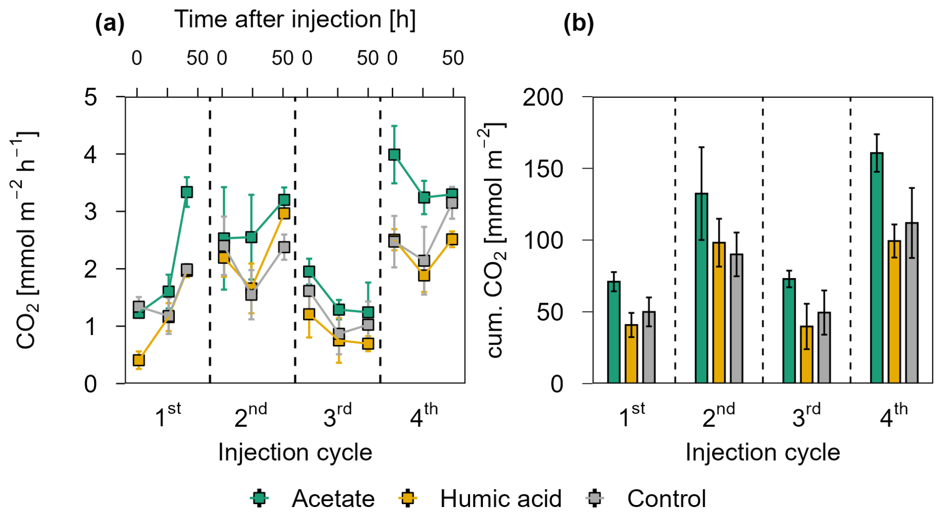
Figure 4 CO₂ release over four OC injection cycles for the acetate, humic acid, and control plots in the pioneer marsh. The dashed lines separate the individual injection cycles. (a) presents individual measured CO₂ fluxes 1.5, 24, and 48 h after injection in CO₂ mmol m⁻² h⁻¹. Acetate (green), humic acid (orange), and NaCl for the control (grey) were injected into the sediment and GHG fluxes were measured directly above the injection spot at the aforementioned time intervals. (b) shows the cumulative CO₂ emissions in CO₂ mmol m⁻² over one injection cycle for each treatment and control. We note here that some variability in the fluxes based on factors such as day/night could not be captured in our sampling approach; we therefore aimed to use a consistent approach and report relative changes rather than emphasize absolute values. For (a) and (b), markers represent mean ± standard error of triplicates for all treatments and the control across injection cycles. For the 1st and 3rd injection cycle for the acetate treatment (both 1.5 h values) were based on duplicate measurements, which is thus also the case for the (b) cumulative CO₂ emission of these cycles.

The CO₂ fluxes showed a positive correlation with air temperature and a moderate positive correlation with the tidal cycle in the pioneer marsh (Table S7). Specifically, CO₂ fluxes were found to be higher as the spring tide receded. Lower CO₂ fluxes were measured during the first and third injection cycles, which occurred close to spring tides.

Further differences between the treatments and control were observed in the DOC concentrations (Fig. S4) and the residual fraction of DOC (Fig. 3a) in the pioneer marsh. Over all four injection cycles, the average DOC concentration in the acetate treated plots did not significantly differ from the control (p > 0.05), while the DOC concentrations of the humic acid treated plots were significantly higher than the concentrations of acetate treated plots and the control plots (p < 0.05, Table S8). These differences are consistent with the residual fraction of DOC (Fig. 3a). Across all four injection cycles, the average residual fraction in the humic acid treatment was significantly higher compared to the acetate treatment but significantly lower than the Br⁻ residual fraction (p < 0.002, p < 0.001 respectively, Table S5). No difference in the TOC content was found between treatments and control in both depths. The content ranged from 0.9 ± 0.1 % to 1.2 ± 0.1 % in the upper 5 cm, with a slight decrease at lower depth (Table S9).

In addition to the gas fluxes, we also measured DIC and pH of the porewater for each treatment and control for each injection cycle (Fig. S5). As the differences in the CO₂ fluxes were more pronounced and our focus was on GHG release, we only present and later discuss these data.

Effect of organic carbon input on the geochemistry of porewater and sediment

In the pioneer marsh, acetate treated plots had significantly higher aqueous Fe(II) concentrations compared to humic acid and control plots when considering the average concentration across all injection cycles (acetate vs. humic acid p=0.007 and vs. control p=0.002, Table S10). Although the differences were not always statistically significant for the individual cycles, the Fe(II) concentration in the porewater of the acetate treated plots was consistently higher (Fig. 5a): 1st cycle 124.52 ± 9.44 µM, 2nd cycle 114.20 ± 19.98 µM, 3rd cycle 114.54 ± 23.80 µM, and 4th cycle 88.08 ± 24.58 µM. Humic acid treated plots and the control plots showed similar aqueous Fe(II) concentrations. For humic acid treated plots the aqueous Fe(II) concentration ranged between 53.36 ± 9.05 µM (2nd cycle) and 79.96 ± 22.16 µM (1st cycle), and for the control between 55.69 ± 8.04 (2nd cycle) and 96.01 ± 36.61 µM (1st cycle) (Fig. 5a).

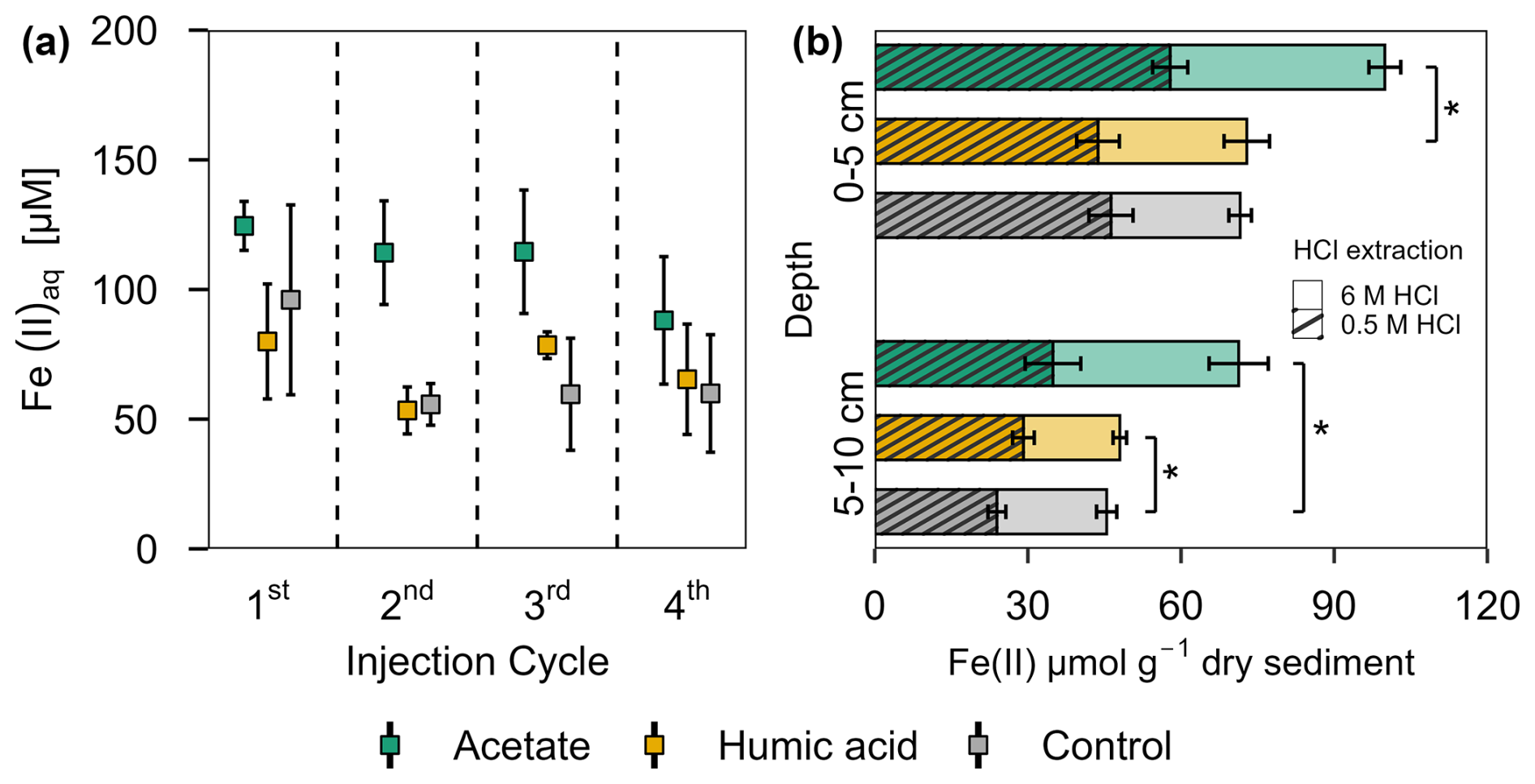
Figure 5 Ferrous iron in (a) porewater and (b) solid phase from acetate and humic acid treated plots and the control plots in the pioneer marsh. (a) Aqueous ferrous iron (Fe(II)_aq) [µM] sampled after each injection cycle (cycles are separated by the dashed line). Triplicates for each treatment and control for each injection cycle were collected and mean ± standard error is shown. (b) HCl extractable Fe(II) content [µmol g⁻¹ dry sediment] at two different depths (0–5 and 5–10 cm) sampled at the end of all four injection cycles. Different colour coding was used for contrasting treatments: acetate treatment (green), humic acid treatment (orange), and control (grey). Striped bars represent poorly crystalline Fe(II) (0.5 M HCl extraction) and solid bars higher crystalline Fe(II) (6 M HCl extraction). The 0.5 M HCl extract was subtracted from the 6 M HCl extracted fraction to separate poorly and higher crystalline Fe(II). Significance is denoted for the 0.5 M HCl extraction. Statistical details are given in the Supplement (Table S11), significance level ^* p < 0.05. For each treatment and control, each spatial triplicate (n=3) was analyzed in triplicate (total n=9) for each depth (0–5 and 5–10 cm); results are presented as mean ± standard error.

A similar trend can be seen in the solid phase for the HCl extractable Fe(II), for both extractions approaches (0.5 M and 6 M HCl) (Fig. 5b). Comparing the poorly crystalline Fe(II) fraction, the acetate treatment had the highest Fe(II) content compared to the humic acid treatment and the control at both depths. Acetate treated plots showed an Fe(II) content of 57.87 ± 3.44 µmol g⁻¹ sediment in the upper 5 cm and 34.91 ± 5.45 µmol g⁻¹ sediment from 5–10 cm. Humic acid and control plots had similar levels of Fe(II): for the humic acid plots, the content in the upper 5 cm was 43.74 ± 4.18 µmol g⁻¹ sediment and from 5–10 cm, it was 29.13 ± 2.12 µmol g⁻¹ sediment. The control plots showed 46.28 ± 4.32 µmol g⁻¹ sediment in the upper 5 cm and 23.93 ± 1.75 µmol g⁻¹ sediment between 5–10 cm. We observed the same trend for the higher crystalline Fe(II) content. The acetate treatment had the highest contents with 42.04 ± 3.12 µmol g⁻¹ sediment (0–5 cm) and 36.38 ± 5.79 µmol g⁻¹ sediment compared with humic acid or control plots. For both depth and crystallinities, the acetate treatment showed significantly the highest content, in nearly all comparisons to the humic acid or control plots (Table S11). Except for poorly crystalline Fe(II) at 5–10 cm depth, humic acid and control plots did not differ significantly (Table S11).

No consistent difference was detected in S(II)_tot in the porewater of the pioneer marsh (Fig. S6a). The S(II)_tot concentrations were in the same range: acetate from 3.16 ± 0.01 µM (4th cycle) to 5.59 ± 1.21 µM (1st cycle), humic acid from 3.0 ± 0.11 µM (4th cycle) to 6.34 ± 1.56 µM (1st cycle) and control from 3.63 ± 0.34 µM (1st cycle) to 4.39 ± 1.13 µM (4th cycle). Also, statistical analysis did not reveal a difference between the different treatments and control S(II)_tot averaged over all cycles (p > 0.05). Similarly, AVS measurements of the solid sulfide species showed no difference between treatments and the control (Fig. S6b). In the upper 5 cm, contents were similar (acetate: 6.13 ± 1.40 µmol g⁻¹ sediment, humic acid 3.89 ± 1.19 µmol g⁻¹, and control 7.37 ± 1.76 µmol g⁻¹ sediment). Similar contents were measured at 5–10 cm depth, with no coherent trend between the layers.

Effect of organic carbon input on microbial growth and metabolic activity

The impact of the added OC on the bacterial community was analysed by qPCR. The analyses were based on DNA (microbial abundance) and RNA (metabolically active microorganisms). The results show the gene copies of both treatments normalized to the control as log₂ fold change (log₂ FC) (Fig. 6). Statistics are based on the absolute gene copy numbers (Fig. S7). For the acetate treated plots a significantly higher bacterial 16S rRNA gene copy number (DNA- and RNA-based) was measured compared to the control plots across all analysed depths (Fig. 6a; p < 0.05). In comparison to the control, DNA-based bacterial 16S rRNA gene copies increased by a factor of 0.4 ±  0.07 (log₂ FC) under acetate treatment and their potential activity, indicated by RNA, increased by 1.58 ± 1.46 log₂ FC in the upper 5 cm. This remained similar at the depth of 5–10 cm, with an increase in DNA-based 16S rRNA gene copies by 0.43 ± 0.09 log₂ FC and an increase in activity (RNA) by 5.09 ± 1.86 log₂ FC. For the comparison between plots amended with humic acid and the control, variations were observed but no significant differences were measured (p > 0.05). Microbial activity (RNA) of Geobacter spp., were higher in the acetate and humic acid treatment compared to the control in the upper 5 cm, however, slightly over the significance criterion (Fig. 6b; p=0.051, p=0.057, respectively). For the acetate treated plots, the activity (RNA-based) of Geobacter spp. was higher compared to the control by a factor of 0.98 ± 0.49. The humic acid treatment also had upregulated activity by a factor of 0.72 ± 0.31. The higher microbial activity of Geobacter spp. remained significantly enhanced (p=0.008) for the acetate treatment compared to the control at the lower depth (RNA-based: log₂ FC: 0.66 ± 0.15), too. The addition of OC did not affect the microbial activity (RNA) of dsrA genes at both depths (Fig. 6c) in the pioneer marsh. However, the abundance (DNA) of dsrA genes in the upper layer was significantly higher for both treatments (acetate p=0.006, humic acid p=0.015). Absolute gene copy numbers are given in Supplement, Fig. S7 and statistical details in Table S12.

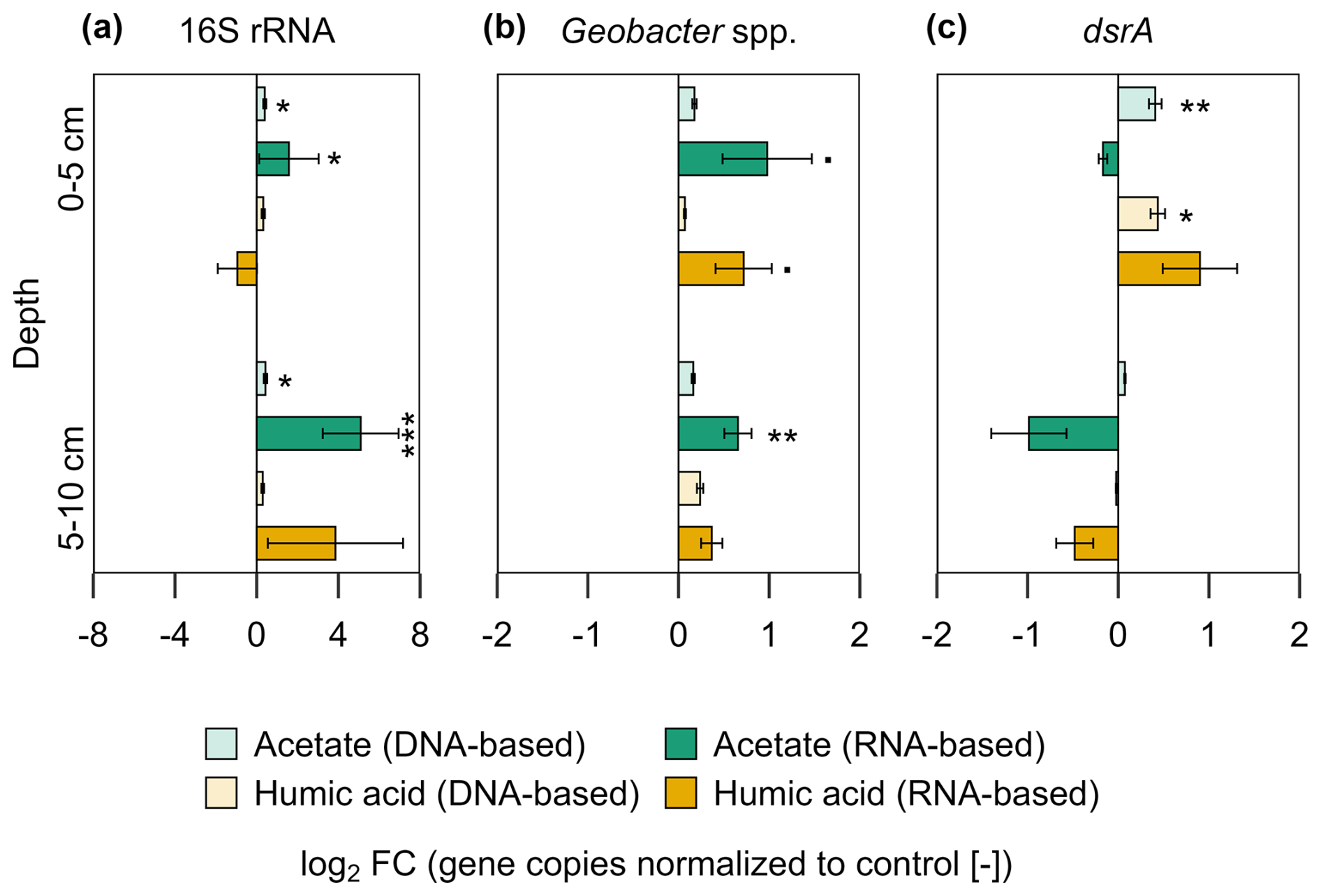
Figure 6 Bacterial gene copy numbers of (a) 16S rRNA, (b) Geobacter spp., and (c) dsrA for acetate and humic acid treatment normalized to the control in the pioneer marsh. The values are represented as log₂ fold change (FC). Values > 0 indicate an upregulation while values <0 indicate downregulation of the genes compared to the control (acetate in green, humic acid in orange). DNA-based numbers are given in lighter colours and RNA-based in darker colours. Statistical differences in the absolute gene copy numbers are indicated as stars in the figure: significant codes are p=0.05, ^* p≤0.05, ${}^{**}$ p≤0.01, and ${}^{***}$ p≤0.001. Absolute gene copy numbers given in Supplement, Fig. S7. Sample sizes include triplicates of each treatment and control at both depths, represented as mean ± standard error (exception of duplicate measurements for 16S rRNA-based humic substances (5–10 cm) and 16S rRNA-based control (0–5 cm)).

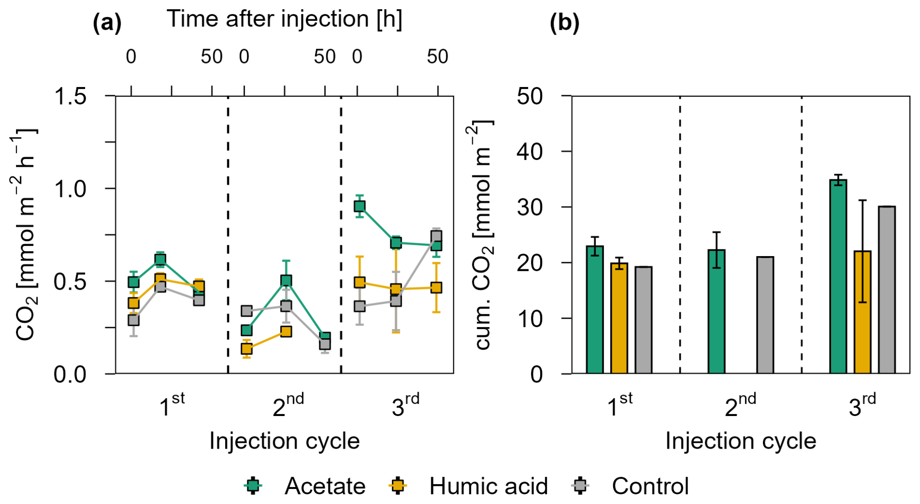
Figure 7 CO₂ release over three injection cycles for the acetate and humic acid treated plots and the control plots in the intertidal flat. (a) CO₂ fluxes after 1.5, 24, and 48 h after injection in CO₂ mmol m⁻² h⁻¹ over three injection cycles. The dashed lines separate the individual injection cycles. In the 2nd injection cycle, fluxes in the humic acid treatment are only displayed at 1.5 and 24 h post injection due to missing data. Acetate (green), humic acid (orange), and NaCl for the control (grey) were injected into the sediment and GHG fluxes were measured directly above the injection spot at the aforementioned time intervals. (b) presents the cumulative CO₂ release in mmol CO₂ m⁻² over one injection cycle for each treatment and control. Due to missing values for humic acid amended plots in the second injection cycle, cumulative emissions could not be calculated. For the same reason, standard errors of the control plots are also not available. For (a) and (b), markers represent the mean ± standard error of triplicates for all treatments and the control across injection cycles, except where missing values for CO₂ release occurred due to nonlinear CO₂ release during the gas sampling incubation time. (a) duplicate measurements are reflected for the 1st injection cycle for the control (1.5 and 24 h), for the 2nd injection cycle for the acetate treatment and control (48 h), and the 3rd injection cycle for the acetate treatment and control (1.5, 24, and 48 h). Single measurement values are shown for the control in the 1st (48 h) and 2nd (1.5 h) injection cycle. For (b), cumulative CO₂ emissions, the acetate treatment shows duplicate measurements for the 2nd and 3rd injection and for the control, only single values are reflected.

3.2.3 Effect of organic carbon input in the intertidal flat

Carbon dioxide release

Figure 7a presents the CO₂ release from the intertidal flat over three injection cycles 1.5, 24, and 48 h post injection. Acetate treated plots released the highest CO₂ in all three injection cycles compared to the humic acid and the control plots. Similar to the pioneer marsh, no strong differences were observed between humic acid treated plots and the control plots. Consistently, the maximum cumulative CO₂ emissions were observed in the acetate treated plots (Fig. 7b). Due to nonlinearity of CO₂ release over the incubation time of gas sampling, some data points are missing; therefore, statistical comparison of CO₂ release between treatments and the control was not done. Nevertheless, plots amended with acetate consistently showed higher CO₂ releases across all injection cycles. Methane was not detected in the fluxes of any treatment in the intertidal flat plots (lower than detection limit (0.28 ppm); Table S3). Similar to the pioneer marsh, we focus here on CO₂ data although DIC and pH were measured (Fig. S8).

No difference in the DOC concentrations between the treatments and the control were measured (Fig. S9). Similarly, no difference was measured between the residual fraction (recovery of injected DOC) between acetate and humic acid treatments (Fig. 3b). The TOC content among the treatments and the control was also in the same range (0.4 %–0.5 %) (Table S9).

Effect of organic carbon input on the geochemistry of porewater and sediment

In the intertidal flat, aqueous Fe(II) concentrations ranged from 9.25 ± 0.21 to 24.82 ± 4.50 µM in both treatments and the control, with no significant differences (p > 0.05) (Fig. S10a). Additionally, no difference between the treatments and the control was detected in the solid phase for both crystallinities (0.5 and 6 M HCl extraction) and depths. In the upper 5 cm, the content of the poorly crystalline Fe(II) ranged from 18.28 ± 1.28 to 19.60 ± 0.88 µmol g⁻¹ sediment among all treatments and control, while in the deeper layer, the range was from 18.11 ± 0.71 to 24.59 ± 1.22 µmol g⁻¹ sediment. The content of the higher crystalline Fe(II) ranged from 11.68 ± 0.99 to 20.06 ± 3.64 µmol g⁻¹ sediment in the upper 5 cm and from 12.98 ± 1.03 to 17.50 ± 2.75 µmol g⁻¹ sediment at a depth of 5–10 cm (Fig. S10b).

For porewater S(II)_tot, no large differences were measured between the treatments and control in the intertidal flat. The concentrations of both treatments and the control were in a similar range over all injection cycles, 0.62 ± 0.01 to 1.73 ± 0.67 µM S(II)_tot (Fig. S11). In contrast, the AVS in the solid phase exhibited a significant difference between the treatments and the control (Fig. 8). Higher AVS contents were measured in the acetate plots. This difference was strongly pronounced in the upper 5 cm in the acetate plots relative to the setups amended with humic acid and the control (p < 0.001 and p=0.007, respectively, Table S13). AVS content in the upper 5 cm was 5.38 ± 0.57 µmol g⁻¹ sediment from the acetate plots, 2.03 ± 0.28 µmol g⁻¹ sediment from the humic acid plots, and 3.40 ± 0.35 µmol g⁻¹ sediment from the control. In the deeper layer (5–10 cm), the differences between treatments and control were statistically negligible (p > 0.05).

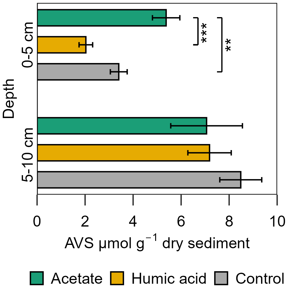
Figure 8 Acid volatile sulfide (AVS) in the solid phase sampled at the end of the experiment for the acetate and humic acid treated plots and the control plots in the intertidal flat. AVS [µmol g⁻¹ dry sediment] content of the solid phase from the different treatments (acetate in green, humic acid in orange) and control (grey). Significance is denoted for the upper sediment layer (0–5 cm), deeper layer no statistically significant difference occurred. Statistical details are given in the Supplement (Table S13), significance level ^* p < 0.05, ${}^{**}$ p < 0.01, and ${}^{***}$ p < 0.001. Each spatial triplicate (n=3) was analyzed in triplicates (total n=9) for each treatment and the control at both depths; results are presented as mean ± standard error.

Effect of organic carbon input on microbial growth and metabolic activity

In the intertidal flat, an increase in DNA- and RNA-based gene copy numbers of the bacterial 16S rRNA gene was detected in the acetate treatment compared to the control at both depths (0–5 and 5–10 cm) (Fig. S12a). This increase was significant for DNA and RNA in the upper layer and remained significant for RNA in the lower layer (p=0.008, p=0.01, and p=0.008, respectively). The acetate treatment showed a 3.62 ± 2.41 log₂ FC increase in the metabolic activity (RNA) of the total microbial community compared to the control in the upper layer and an increase of 2.73 ± 1.41 log₂ FC from 5–10 cm. For Geobacter spp. (Fig. S12b) the RNA-based gene copies were significantly higher compared to the control (p < 0.001) by a factor of 0.6 ± 0.10 in the upper 5 cm. No significant increase in the RNA-based copy numbers of dsrA genes in both depths (Fig. S12c) were observed; however, we detected slightly higher RNA-based dsrA gene copies in the acetate treatments (0.33 ± 0.06 log₂ FC) compared to the control in the upper layer. Absolute gene copy numbers are presented in Fig. S13 and statistical details in Table S14.

4 Discussion

4.1 Geochemistry at the study site

Porewater and solid phase measurements from the push cores showed availability of electron acceptors (O₂, Fe(III), and SO${}_{\mathrm{4}}^{\mathrm{2}-}$) at different depths in both the pioneer marsh and intertidal flat. Based on microsensor measurements during low tide, we observed O₂ concentrations in the top 2 mm decreasing with depth, from 131.02 ± 26.49 to 0.18 ± 0.12 µmol L⁻¹ in the pioneer marsh, and in the intertidal flat from 155.17 ± 12.71 to 0.62 ± 1.10 µmol L⁻¹, reaching 0 µM below that depth. This finding directly affects which biogeochemical processes occur below this depth. Other studies conducted in comparable ecosystems have indicated that during high tide and/or daytime, O₂ penetrates deeper into the sediment (de Beer et al., 2005; Bosselmann et al., 2003), but reducing conditions may prevail underneath and that the depth of O₂ penetration might be influenced by sediment grain size. Both zones in our study showed a high proportion of fine particles (silt: 29.0 ± 5.0 to 38.7 ± 2.5 % and clay: 9.5 ± 5.5 to 19.7 ± 8.1 %). Such a size distribution retains more water (Novák and Hlaváèiková, 2019), resulting in water-filled pore spaces even during low tide, which limits gas exchange. We suggest that the lack of O₂ penetration beyond 2 mm at our study site results from the presence of fine particles. Despite differences in the duration and magnitude of inundation between the zones, the depth of O₂ penetration remained similar, indicating that these factors do not influence O₂ penetration depth and that reducing conditions prevail beyond the upper millimetres during both tidal conditions. We do not exclude that the presence of sparse vegetation in the pioneer marsh compared to no vegetation in the intertidal flat may cause differences in the intrusion of O₂ into the sediment (Koop-Jakobsen et al., 2017; Maricle and Lee, 2002). However, we did not detect this difference in our O₂ measurements. In addition to plants, benthic organisms such as worms may introduce O₂ into the sediment and influence the biogeochemical cycling in the sediment (Huettel et al., 2014). As worms were present in both zones, it is likely that they play a role in O₂ penetration and re-oxidizing of reduced Fe(II) or sulfide species (Fig. S14a–d). We expect that this effect is not substantially different for the two zones, as no large qualitative difference in the presence of worms was observed visually.

Below the oxic zone, alternative electron acceptors were present. We used Fe(II) porewater data as an indicator of Fe(III) reduction. A decrease in the aqueous Fe(II) from 267.49 ± 66.77 to 31.41 µM Fe(II) in the pioneer marsh and from 19.93 ± 16.15 to 7.20 ± 2.89 µM Fe(II) in the intertidal flat was measured over 25 cm. Based on the presence of aqueous Fe(II), we assumed that Fe(III) reduction is likely occurring in both zones, which is less pronounced in the intertidal flat. The observed decreasing trend over depth has been commonly seen in other studies of coastal sediment (Moeslundi et al., 1994; Lowe et al., 2000). It suggests a depletion of bioavailable Fe(III) with depth and/or removal of aqueous Fe(II). Aqueous Fe(II) can precipitate with sulfide, which forms through SO${}_{\mathrm{4}}^{\mathrm{2}-}$ reduction deeper in the sediment when more thermodynamically favourable electron acceptors are exhausted (Jørgensen et al., 2019). The Fe(II) porewater concentrations are in the range of other studies from salt marshes, especially for the pioneer marsh (0–800 µM) (Kostka et al., 2002b; Seyfferth et al., 2020). Concentrations of the intertidal flat are on the lower end of the studies mentioned above. Ferrous iron was the predominant iron species in the solid fraction extracted by 0.5 M HCl in both zones. Manganese(IV) as an electron acceptor was not further considered as the total manganese concentration from the study site is 5 µmol g⁻¹ sediment (Kubeneck et al., 2025), and thus relatively low in comparison to the total iron concentration.

Sulfate has a major role in the oxidation of OC as an important electron acceptor in coastal wetlands due to its frequent supply via the incoming seawater. We observed a slight decrease in SO${}_{\mathrm{4}}^{\mathrm{2}-}$ over a depth of 20 cm which was more distinct in the intertidal flat, as seen in the sulfate to chloride ratio (Fig. S2a). This suggests some SO${}_{\mathrm{4}}^{\mathrm{2}-}$ reduction in the upper 20 cm. A similar pattern was observed at a comparable site where Fe(II) predominates over total iron and porewater SO${}_{\mathrm{4}}^{\mathrm{2}-}$ concentration decreases with depth, albeit with slightly higher SO${}_{\mathrm{4}}^{\mathrm{2}-}$ concentrations (Kostka et al., 2002b). The relatively high levels of SO${}_{\mathrm{4}}^{\mathrm{2}-}$ at all tested depths (> 50 cm), supported the absence of detectable CH₄ dissolved in the porewater or as an efflux. This is consistent with past studies such as Martens and Berner (1974) who stated that if more than ∼ 10 % of seawater SO${}_{\mathrm{4}}^{\mathrm{2}-}$ is still present, CH₄ is not produced, as a thermodynamically more favourable electron acceptor is available (Schlesinger and Bernhardt, 2013b). We examined different possible explanations for the lack of detected CH₄ as we could not entirely exclude that CH₄ was produced further down in the sediment and oxidized via anaerobic methane oxidation (AOM), as observed in some coastal wetlands (Capooci et al., 2024; La et al., 2022; Wang et al., 2019), or by lateral transport to surrounding tidal channels (Trifunovic et al., 2020). We did not measure any CH₄ as a efflux or in the porewater over multiple field campaigns, similar to a study conducted at the same study site by Kubeneck et al. (2025). We considered the sensitivity of detection: the detection limit for porewater CH₄ was 0.53 ppm (Table S3) which corresponds to 1.13 µmol L⁻¹ based on our sampling method. We would expect that methane, if produced within the depths examined here, would be above this concentration as porewater concentrations of CH₄ in wetlands slightly inland within the Elbe estuary were much higher (0.16 to 2.46 mmol L⁻¹, Kubeneck et al., 2025). It is possible that trace amounts of CH₄ (ppb) were present below the detection limit. The few other studies that have detected CH₄ in the Wadden Sea were at depths where SO${}_{\mathrm{4}}^{\mathrm{2}-}$ was largely depleted (Røy et al., 2008; Wu et al., 2015), which is not the case in our study. Furthermore, the absence of an observed decrease in SO${}_{\mathrm{4}}^{\mathrm{2}-}$ concentration, particularly in the pioneer marsh, suggest a lack of AOM until 50 cm, as CH₄ and SO${}_{\mathrm{4}}^{\mathrm{2}-}$ are consumed in a 1:1 stochiometric ratio during sulfate AOM. Thus, our results indicate that CH₄ production and consumption are unlikely until 50 cm. Below these depths, these processes may be occurring. Further analysis of the microbial community and/or CH₄ injection experiments would help to determine if methanogenesis and AOM occur at lower depths. Based on the high concentrations of SO${}_{\mathrm{4}}^{\mathrm{2}-}$ with relatively low changes with depth as well as the lack of detectable CH₄, we suggest that electron acceptors may not be limiting the microbial turnover of OC and release of CO₂ in our study. To our knowledge, this is rarely reported for coastal wetlands and not commonly expected for terrestrial ecosystems. Here, we caution that further measurements of rates of electron acceptor turnover and/or incubation experiments are needed to unambiguously exclude an electron acceptor limitation.

We also considered the OC sources in the system: porewater DOC and solid phase TOC. The TOC content was ∼ 1 % and decreased with depth in both zones. A decreasing trend over depth was also seen in the DOC concentrations. The decrease of OC with depth indicates decomposition and has been commonly observed in other studies (Hansen et al., 2017; Mueller et al., 2019). The range in TOC and DOC concentrations are at the lower end of comparable ecosystems with the main differences in the upper centimetres (Gribsholt and Kristensen, 2003; Hansen et al., 2017; Mueller et al., 2023).

4.2 In situ organic carbon manipulation experiment

4.2.1 Validation of the experimental setup

Bromide, as an inert tracer, was injected along with the OC/control solution into each experimental cylinder for each injection cycle. This allowed us to follow the distribution and retention time of the injected solution over one injection cycle. The Br⁻ concentration over each injection cycle was higher than the background Br⁻ concentration (Fig. 3, S3a, b), indicating that the injected solution was partially retained within the experimental cylinder over one injection cycle. The observed decrease in Br⁻ concentration over one injection cycle, more pronounced in the intertidal flat (Fig. S3b), was likely due to flushing out by tidal water and belowground water movement. We observed a slightly lower retention of Br⁻ in the intertidal flats compared to the pioneer zone. We attribute this difference to the higher sand fraction in the intertidal flats, which likely increased permeability and led to stronger tidal flushing of the injected solution as well as subject to greater tidal inundation.

As the Br⁻ concentrations and the respective calculated residual fractions were similar for each cycle (Fig. 3), we infer that there was no residue of Br⁻ and thus no injected OC was carried over between cycles. Furthermore, the retained Br⁻ was similar between the plots of a treatment within one zone, indicating similar belowground conditions within one zone and thereby validating the experimental setup. By placing the experimental plots outside of vegetated areas in the pioneer marsh, we tried to avoid geochemical influence on the sediment by plants. However, it is possible that benthic organisms such as worms may have influenced the biogeochemistry in both the pioneer marsh and intertidal flat, causing some variability.

4.2.2 Effect of organic carbon input in the pioneer marsh

Carbon dioxide fluxes

To test our hypothesis that that microbially mediated CO₂ release is OC limited in the pioneer marsh, we injected two different OC sources into the sediment and monitored the subsequent release of CO₂ 1.5, 24, and 48 h post injection. We observed that acetate treated plots emitted the highest CO₂ throughout the experiment (Fig. 4). No difference in the CO₂ release was measured between the humic acid treatment and the control despite the additional availability of OC. This is supported by the work of Gunina and Kuzyakov (2022) who showed that reduced and complex organics in soils are predominantly thermodynamically preserved due to insufficient energy yield upon decomposition. Humic acid, as complex OC, may be thus preserved in our study, as reflected in higher DOC concentrations. In contrast, acetate, with a simpler chemical structure, is favourable for microbial decomposition even under reducing conditions (Boye et al., 2017; LaRowe and Van Cappellen, 2011) and thus could be readily utilized and oxidized to CO₂. Notably, plots treated with humic acid received the same OC concentrations as the acetate plots, indicating that OC composition is crucial for the CO₂ release from minerogenic pioneer marshes. Based on the geochemistry at the field site, which suggested that the ecosystem is limited by the availability of OC, the results from the in situ experiment further support our hypothesis, while simultaneously highlighting the importance of OC composition. This is contrasting to other terrestrial wetlands, which are characterized by a depletion of TEAs (Schlesinger and Bernhardt, 2013b).

The increased turnover of acetate to CO₂ relative to humic acid is also evidenced in the DOC concentrations (Fig. S4) and the retention fraction of both DOC sources (Fig. 3a). Although the same mass of OC was added to both treatments, the DOC concentrations in the acetate plots were significantly lower than that in the humic acid plots, suggesting that more acetate was utilized, reflected in higher CO₂ release. However, this result does not explain the lower retention of DOC relative to the retention of Br⁻ from the humic acid plots (Fig. 3a). This suggests that in addition to flushing out, adsorption likely occurred. Previous studies have shown that minerals within the subsurface adsorb organic compounds (Kahle et al., 2003; Kleber et al., 2021). This adsorption may be preferential, favouring more aromatic and high molecular weight compounds, particularly when metal (oxyhydr)oxides and clay minerals are present (Kaiser and Guggenberger, 2000; Lv et al., 2016; Voggenreiter et al., 2024). Based on the results of our study and a previous study conducted at the same site (Kubeneck et al., 2024), both iron(oxyhdyr)oxides and clay minerals are present. As adsorption suppresses the decomposition of OC (Kleber et al., 2021), we speculate that the lower retention fraction of humic acid compared to Br⁻ was primarily due to adsorption onto the sediment rather than decomposition. This is consistent with the CO₂ fluxes: humic acid treated plots showed lower retention fractions compared to the Br⁻ retention fractions, however, the CO₂ fluxes were comparable to the control. This suggests that little to no decomposition occurred and that adsorption was the dominant process. It is worth noting that anoxic decomposition of humic acid is generally possible but the turnover time would have exceeded the duration of the experiment (Lipczynska-Kochany, 2018). These results highlight that it is not only the presence of OC that affects short-term OC release from coastal wetlands; the composition of OC is the primary determining factor.

Furthermore, it is important to note that the OC concentrations used in this experiment are higher than those expected for naturally occurring OC inputs, such as root exudates, which are typically released at lower concentrations with a continuous input. Thus, upscaling the enhanced CO₂ fluxes measured in our study might result in overestimation of CO₂ release from minerogenic salt marshes. Our findings rather reveal, on a process level, that the addition of labile OC stimulates microbially mediated CO₂ release. Enhanced CO₂ release from the acetate amended plots was measured at nearly all sampling time points (1.5, 24, and 48 h) without a clear trend, while the concentration of the inert tracer showed a slight decrease over the same period (Fig. S3) – indicating slight dilution and flushing of the injected OC. This suggest that the elevated CO₂ release was driven by enhanced availability of labile OC independently of its concentration. These findings allow us to generalize that the system is likely limited by labile OC availability, regardless of the concentration; however, further work should quantify how the magnitude of CO₂ promotion corresponds to OC concentration, particularly under low, naturally sustained OC input rates. In conclusion, we can reliably predict the direction of increased OC inputs to minerogenic salt marshes, but further studies are needed to predict the specific long-term magnitude of changes in the carbon cycle in these ecosystems.

Enhanced microbial Fe(III) reduction leads to higher CO₂ release

This section combines the observed effect of OC input on the geochemistry of the porewater and sediment with the microbial growth and metabolic activity and links them to the CO₂ release from the pioneer marsh. The bacterial 16S rRNA gene copy number, an indicator of the total bacterial abundance, was significantly higher in the acetate treatment compared to the control for both DNA and RNA at both depths. This suggests greater bacterial abundance and metabolic activity, which likely led to higher CO₂ fluxes from these plots. No significant difference was noticeable in the 16S rRNA gene copy number between plots amended with humic acid and the control. Overall, the 16S rRNA gene copy numbers (DNA) are in the range of other studies from coastal wetlands and marine sediment (Petro et al., 2019; Zhou et al., 2017).

The enhanced metabolic activity in the acetate treated plots is further reflected in the elevated aqueous and solid phase Fe(II). The acetate treatment showed higher aqueous Fe(II) concentrations in all four injection cycles, while no significant difference was observed between the humic acid and control plots. In the solid phase, the Fe(II) content was the highest in the acetate treatment. Thus, the higher expression of Geobacter spp. in the acetate treated plots corresponds well to our geochemical observations. Geobacter spp. have been shown to use acetate as a carbon source to gain energy (Coates et al., 1996). The higher Fe(II) levels observed in both aqueous and solid phase of acetate treated plots along with elevated Geobacter spp. gene copies indicate that Fe(III) reduction was stimulated by increased availability of labile OC.

Ferric iron and SO${}_{\mathrm{4}}^{\mathrm{2}-}$ reduction have been reported as OC decomposition processes in salt marshes (Hyun et al., 2007; Kostka et al., 2002a; Lowe et al., 2000). Sulfide concentrations in the porewater as well as in the solid phase gave evidence that SO${}_{\mathrm{4}}^{\mathrm{2}-}$ reduction occurred; however, no differences between the treatments and controls were seen. The functional gene analysis provided further evidence for this, as sulfate-reducing bacteria (SRB) were present (absolute gene copy numbers in Supplement Fig. S7); however, none of the treatments led to an increase in their metabolic activity compared to the control (Fig. 6). Thus, we speculate that the higher CO₂ release from the acetate treatment was mainly driven by the enhanced Fe(III) reduction and not by SO${}_{\mathrm{4}}^{\mathrm{2}-}$ reduction. Our finding that acetate is utilized follows the conventional thermodynamic sequence of iron reduction being more favorable than SO${}_{\mathrm{4}}^{\mathrm{2}-}$ reduction (Schlesinger and Bernhardt, 2013b) – even if the concentrations and availability of SO${}_{\mathrm{4}}^{\mathrm{2}-}$ were much higher.

4.2.3 Effect of organic carbon input in the intertidal flat

Carbon dioxide fluxes

Adding OC to the intertidal flat, a zone more influenced by tides than the pioneer marsh, resulted in CO₂ trends similar to the pioneer marsh. Acetate addition led to a noticeable increase in CO₂ fluxes. In contrast, the CO₂ fluxes from the humic acid and control plots were similar. This supports our hypothesis that the electron donor limits CO₂ release from the ecosystem. Moreover, it highlights that irrespective of tidal influence, the system is limited by the availability and composition of OC.

Enhanced microbial activity leads to higher CO₂ release

Total microbial 16S rRNA gene copies were significantly higher in the acetate treated intertidal flat plots compared to the control at both depths (RNA-based), whereas plots amended with humic acid showed no significant difference from the control plots (Fig. S12a). In contrast to the significant increase in Geobacter spp. gene copies, no difference in the aqueous Fe(II) or in the Fe(II) content in the upper sediment layer (0–5 cm) was measured for the acetate treatment, except for a higher Fe(II) content in the deeper sediment layer. Conversely, we measured higher AVS contents in the upper layer for the acetate treatment, but this is not reflected in higher dsrA copies numbers. Based on these mixed results, we consider two hypotheses: (i) acetate promoted increased Fe(III) reduction, which is supported by higher gene copies of Geobacter spp. However, this is not clearly reflected in the Fe(II) data. Furthermore, with increased Fe(III) reduction and a constant SO${}_{\mathrm{4}}^{\mathrm{2}-}$ reduction rate, we would have expected a depletion of S(II)_tot in the porewater of the acetate treatment due to iron-sulfur mineral formation; however, this was not observed. Thus, we consider a second hypothesis that (ii) acetate promoted SO${}_{\mathrm{4}}^{\mathrm{2}-}$ reduction, supported by increased AVS content in the acetate treatment in the upper sediment layer. In contrast, the number of dsrA gene copies was not higher in the acetate treatment. Although a small increase (RNA-based) in the gene copies of dsrA was observed in the upper layer, this was not statistically significant. Additionally, no differences were observed in the S(II)_tot concentrations, which were generally low and should therefore be interpreted with caution. Based on our data, we cannot clearly reject either hypothesis. We therefore suggest Fe(III) and SO${}_{\mathrm{4}}^{\mathrm{2}-}$ reduction both lead to higher CO₂ release, stimulated by higher supply of labile OC in the intertidal flat.

5 Conclusion and Implications

Our study demonstrated that the composition in combination with the concentration of OC can drive the CO₂ release from minerogenic salt marshes typical of the Wadden Sea. Initial porewater and sediment geochemical characterization suggested that microbially mediated CO₂ release is likely not limited by the availability of electron acceptors in both the pioneer marsh and intertidal flat, contrary to what is generally observed in terrestrial wetlands. Overall, our results indicate that the OC composition, rather than the concentration alone, influenced CO₂ release in both succession zones. This suggests that OC composition likely plays a limiting role in microbially mediated CO₂ release from minerogenic salt marshes. We caution here that we did not directly measure TEA reduction rates. Future studies should investigate turnover rates, potentially utilizing isotopes to confirm our findings. The higher CO₂ release observed in the acetate treated plots within the pioneer marsh was accompanied by higher levels of reduced iron. This pattern also corresponded with greater activity of Fe(III)-reducing bacteria in these plots, indicating that microbially mediated CO₂ release resulted from Fe(III) reduction driven by increased labile OC input. The addition of the complex OC (humic acid) did not exceed the CO₂ release of the control, showing that complex OC was not decomposed. Similar trends in CO₂ release were measured for the intertidal flat, further indicating that OC (both in terms of composition and concentration) is a key driver of microbial decomposition of OC to CO₂ for salt marsh systems. We expect that this is particularly relevant in salt marshes similar to ours with a high proportion of fine particles (muddy marshes) relative to marshes with larger particles (sandy marshes).

The results of this in situ study contribute to our understanding of short-term carbon dynamics in minerogenic temperate salt marshes. Labile OC inputs such as root exudates may enhance CO₂ release from minerogenic salt marshes, while complex OC inputs, such as plant fragments, might be sequestered in the sediment rather than degraded and released as CO₂. The controls on OC turnover observed here should be considered when accounting for these ecosystems as carbon sinks and stocks. Also, our results show that the link between OC composition and the release of CO₂, independent of electron acceptor concentrations, is crucial and should be included in process-based modelling of carbon fluxes in these ecosystems (Brown, 2025; Regnier et al., 2013). This will contribute to more accurate predictions of the response of salt marshes to climate change. Further, the in situ experiment simulated a potential increase of short-term OC inputs to the ecosystem, reflecting scenarios associated with climate change such as inundation of previously unflooded areas due to sea level rise and storm surges or eutrophication (van Beusekom, 2005; Esselink et al., 2017; Woth et al., 2006). For example, eutrophication may result in an input of organic matter into the Wadden Sea that is eventually washed onto the coastal sediment. Our study thus provides valuable insight into the consequences of such short-term scenarios for GHG release and highlights that the input of labile OC (e.g., primary production during eutrophication, root exudates) into the sediment of a minerogenic salt marsh results in higher CO₂ releases.