Unexpected quasi-independence of coloured dissolved organic matter absorption from chlorophyll-a concentration in the Southern Ocean

The absorption coefficient of coloured dissolved organic matter (CDOM), a_y, plays a critical role in driving ocean optical properties and thereby light attenuation and light-dependent biogeochemical cycles. In the Southern Ocean (SO), however, a_y remains poorly documented because of the scarcity of in situ measurements and the absence of suitable bio-optical models. To address this gap, we derived a_y in surface waters from the diffuse attenuation coefficient (K_d) derived from radiometric measurements performed by Biogeochemical-Argo floats. Sensitivity analyses using Monte Carlo simulations indicated that the uncertainty of our estimates is mainly driven by the uncertainty in K_d, and is overall ∼ 18 % for a_y at 380 and 412 nm. Our derived a_y vs. chlorophyll-a concentration (Chl) relationships for low-latitude waters are consistent with previously published relationships. They, however, diverge in the SO, with a larger relative contribution of a_y to the absorption budget for clear waters (Chl < ∼ 0.2 mg m⁻³) and the opposite for greener waters, leading to a weaker dependence of a_y on Chl. Lower-than-expected CDOM absorption mostly happens during the austral summer, suggesting significant photobleaching or lower biologically-mediated production. The relative contributions of CDOM and phytoplankton to the absorption budget are also found to diverge from what bio-optical models predict, with implication for interpretation of satellite ocean colour observations in the SO.

1 Introduction

Coloured dissolved organic matter (CDOM) in oceanic waters is the fraction of the dissolved organic matter (DOM) pool that absorbs light in the ultraviolet and visible region of the electromagnetic spectrum. The corresponding absorption coefficient is hereafter denoted a_y (m⁻¹), with the subscript referring to the yellow substance denomination used in previous studies (Morel and Gentili, 2009). CDOM absorption reduces light penetration within the water column, thereby influencing phytoplankton dynamics, nutrient cycling, primary productivity, and the overall biological carbon pump (Nelson and Siegel, 2002; Siegel et al., 2002; Nelson and Siegel, 2013; Mannino et al., 2014). Therefore, it plays a significant role in regulating biogeochemical and photochemical processes within the global carbon cycle (Gruber et al., 2009, 2019; Hauck et al., 2023; Boyd et al., 2024). Accordingly, it is important to quantify the CDOM distribution for better understanding of the biogeochemical processes underlying its variability.

In addition, CDOM absorption in the blue part of the spectrum is superimposed to phytoplankton absorption, which means that accurately quantifying a_y is also of paramount importance to a proper estimate of the phytoplankton chlorophyll-a concentration (Chl, mg m⁻³) from satellite ocean colour measurements, which combine reflectance measurements in several spectral bands including in the blue (generally around 440 nm). A higher (lower) CDOM contribution to absorption in the blue than assumed in semi-analytical ocean colour algorithms will lead to (under)overestimating Chl. Several studies have indeed pointed to significant biases when comparing satellite-derived Chl with field measurements in the SO (e.g., Johnson et al., 2013; Chen et al., 2021) while others did not identify such an issue (e.g., Haëntjens et al., 2017). Atmospheric correction issues have been suggested as a possible reason for these degraded performances in the SO, although only for studies focusing on coastal areas (Salyuk et al., 2025). Therefore, no consensus exists about the reasons for the poor performance of satellite Chl algorithms (e.g., Morel and Maritorena, 2001; Hu et al., 2012) in the SO. Since these algorithms have been developed primarily from low-latitude bio-optical data sets, the question arose as to whether the SO bio-optical properties significantly differ from what they are in low-latitude oceans, making the application of current satellite ocean colour algorithm problematic.

Studies have indeed shown that bio-optical properties of the SO are statistically different from low-latitude waters, both for phytoplankton (Robinson et al., 2021) and non-algal particles (NAP; Li et al., 2024), with impact on the ocean reflectance (Dierssen and Smith, 2000). The role of CDOM absorption as another source of misinterpretation of the satellite ocean colour signal in terms of Chl has not, however, been thoroughly investigated. Therefore, the main objective of this study is to assess whether the relationship between Chl and a_y in the SO differs from other oceanic regions and, if it does, to discuss possible reasons.

Whether CDOM concentration, hence the amplitude of a_y, is high or low in the surface layers of the oceans depend on the balance between CDOM production and losses. In the open oceans, production is essentially local from biological activity, and losses can occur either through photobleaching, biological degradation, dilution through vertical mixing with CDOM-poor waters or enrichment if mixing occurs with CDOM-rich deep waters (Siegel et al., 2005; Nelson and Siegel, 2013; Fichot et al., 2023; Yamamoto et al., 2024). Surface circulation can either lead to increases or decreases of a_y depending on which water masses are advected. These processes occur in all oceans, yet some peculiarities of the SO might lead to a different balance between CDOM production and losses.

The SO is characterized by strong vertical mixing in winter, low photobleaching in the low-irradiance winter yet strong photobleaching in summer when irradiance can be as high as it is in the equatorial belt (Campbell and Aarup, 1989). Phytoplankton populations are different to what they are in low-latitude environments (e.g., Wright et al., 2010). Sea ice melting is another potential source of CDOM (Ortega-Retuerta et al., 2010b) affecting waters in the seasonal ice zone. It is therefore legitimate to expect that this rather peculiar combination of characteristics and processes might lead to changes in the a_y vs. Chl relationship.

While the number of CDOM absorption measurements are increasing in global databases, as for any dynamic variable, in situ observations will always under-sample the ocean. This is even more true in the SO where logistical difficulty and the harsh environment mean that we have extremely limited in situ studies of CDOM. Therefore, addressing our question using ship-based a_y and Chl measurements was not possible. The deployment of autonomous profiling Biogeochemical-Argo (hereafter BGC-Argo) floats in the SO by, e.g., the Southern Ocean Carbon and Climate observations and Modelling (SOCCOM; Sarmiento et al., 2023) or the Remotely-sensed Biogeochemical Cycles in the Ocean (RemOcean; Claustre et al., 2020) programs has dramatically improved the availability of in situ data, and made this study feasible. Here we used floats equipped with radiometers, allowing a semi-analytical derivation of a_y from the diffuse attenuation coefficient of downward irradiance, K_d (m⁻¹). Our method uncertainties were quantified through sensitivity analyses and Monte Carlo simulations. We then compared a_y-related bio-optical properties and relationships between the SO and low-latitude waters to explore potential mechanisms underlying their differing distributions.

2 Data and methods

2.1 Data selection from BGC-Argo floats

We used data from a total of 60 BGC-Argo floats deployed in the SO (south of 40° S in this study) between 29 November 2013 and 2 May 2025, and 211 floats deployed in low-latitude regions (from 40° S to 60° N) from 22 October 2012 to 26 December 2024. These floats are equipped with Seabird CTD sensors for temperature and salinity, Seabird/Satlantic OCR-500 multispectral radiometers collecting downward plane irradiance (E_d(z,λ), µW cm⁻² nm⁻¹) at 380, 412 and 490 nm, and Seabird/WET Labs ECO-series sensors providing the total optical backscattering coefficient at 700 nm(b_b (700), m⁻¹) and chlorophyll fluorescence. Overall, these floats had collected 10 579 (SO) and 38 615 (low latitudes) profiles during the period indicated.

For each of the floats, we first eliminated profiles collected in shallow waters (depth < 200 m) based on the global relief ETOPO1 data base (NOAA, 2009), as well as profiles for which the sun elevation was < 15° at the end of the upcast. Then, for chlorophyll, backscattering and radiometry, we only kept profiles flagged “A” (100 % of good data) or “B” (at least 75 % of good data), as per the nomenclature of the Argo data management team (Argo data management, 2025). For the profiles passing this first screening, only data points with a quality flag set to either 1 (good), 2 (probably good), 5 (value changed) or 8 (interpolated value) were kept.The total of data points flagged either 1 or 2 was from 80 % to 98 % of the entire data set depending on the parameter.

The locations of profiles that passed these quality controls (roughly one third of the total) are displayed in Fig. 1, and the number of profiles eliminated after each step of quality control are summarized in Table S1 in the Supplement. The temporal coverage of the selected profiles across years and months is displayed in Fig. S1 in the Supplement. The distribution of the sun zenith angles is depicted in Fig. S2a, while Fig. S2b shows the irradiance just above the surface for λ= 490 nm, limited to cases within 20 % of the theoretical clear-sky value calculated following Gregg and Carder (1990).

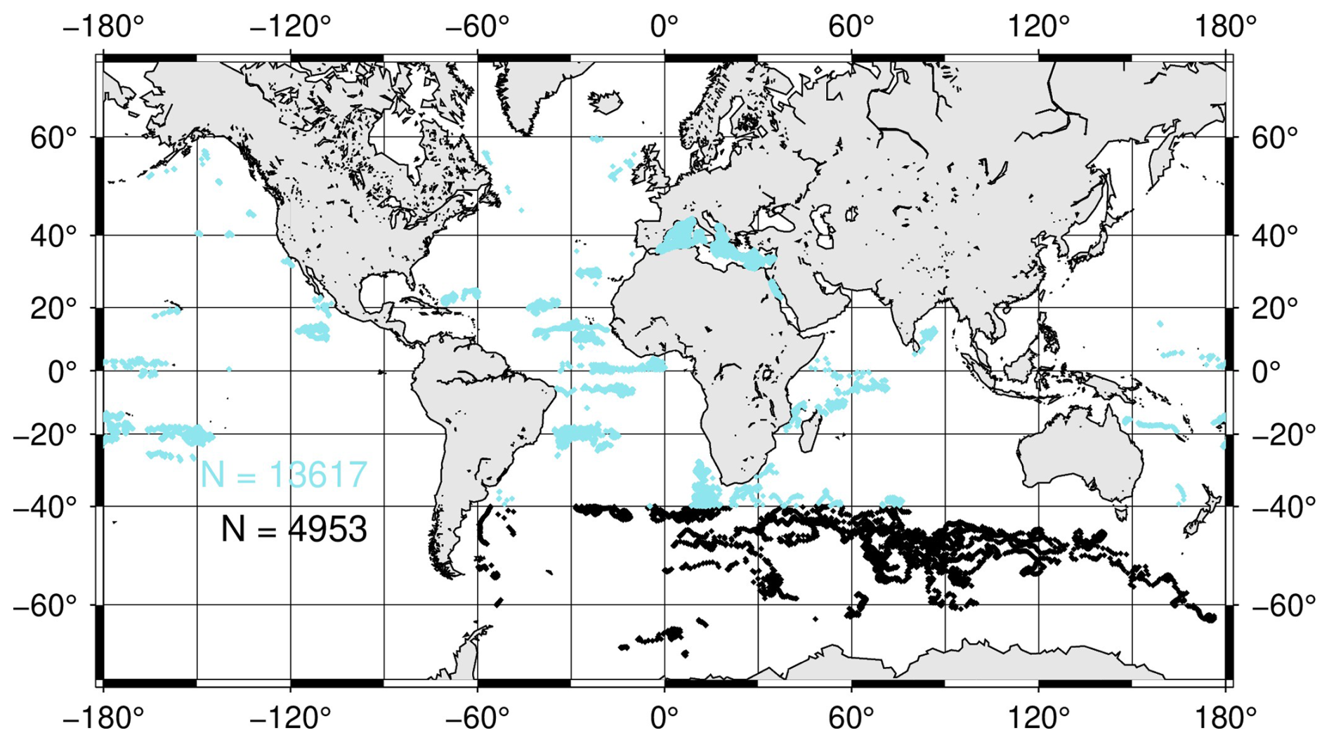
Figure 1 Surface locations of the BGC-Argo float profiles used in this study for the SO (black) and elsewhere (blue), after various screenings have been applied to the full data set (see methods).

2.2 From radiometric measurements to K_d

The overall workflow we used to then process the BGC-Argo data is displayed in Fig. S3. We did not correct the radiometry data for dark deep values, which have been shown to be negligible (Organelli et al., 2016). We checked these values and indeed they were always lower than 10⁻³ mW cm⁻² nm⁻¹, with a distribution centred on 10⁻⁴ mW cm⁻² nm⁻¹.

Then a 4th order polynomial was fitted to the data to clean the E_d(z,λ) profiles from changes due to possible changes in the above-water downward irradiance caused by clouds and from near surface fluctuations generated by waves. This fit was only performed if more than 20 valid data points were available, otherwise the profile was eliminated. This fitting procedure is similar to what Organelli et al. (2016) did, although we did not find it necessary to repeat the 4th order polynomial in order to get smooth profiles.

The K_d were then calculated in three different ways from the fitted E_d profile, to allow a sensitivity study of the K_d value. The first one (K_d(0–20 m)) was calculated from E_d(z= 0⁻) and E_d(z= 20 m). This approach mimics the methodology used in most of the field data sets by Morel (1988) and later revised by Morel and Maritorena (2001) (hereafter MM01), and it is taken here as the reference for the low-latitude environments. At that time, profiling radiometers were not yet available; instead, radiometers were deployed using winches and stabilized at successive depths where measurements were collected. A depth of about 20 m was typically chosen, as irradiance fluctuations were sufficiently dampened to ensure reliable E_d measurements. The second K_d calculation (K_d(Z_pd) was similar but used E_d at the first optical depth (Z_pd) instead of at 20 m. This depth was calculated for each wavelength and corresponds to the point where E_d is reduced to $\mathrm{1}/e$ of its below-surface value. At this stage, we added another quality control by eliminating profiles when Z_pd deviated by more than a factor of 2.5 (either greater or lower) from the value predicted from Chl using MM01. The third calculation took the mode of the distribution of local K_d values, computed at each measurement depth within successive 5 m intervals from just below the surface down to the first optical depth. K_d (0–20 m) is the one used in subsequent analyses.

2.3 Chlorophyll, backscattering and mixed-layer depth from BGC-Argo floats

The Chl values delivered by the BGC-Argo program are derived from chlorophyll fluorescence profiles corrected for possible non-photochemical quenching (Xing et al., 2018; Schmechtig et al., 2023), then scaled to Chl using manufacturers calibration parameters and further divided by a factor of 2 following recommendation by Roesler et al. (2017). A similar correction of the fluorescence-to-Chl ratio was recommended for SO phytoplankton by Schallenberg et al. (2022) with, however, a factor of 3.79 instead of 2, which we have used here. Each Chl and total backscattering profiles were adjusted by shifting the whole profile so that the average value between 200 and 400 dbar equals the mode of the distribution of deep values calculated over the same depth range from all profiles of all floats. This adjustment was performed to account for the potential bias between different measurement technologies and for possible instrument drift. These deep values were $\mathrm{5.5}\times {\mathrm{10}}^{-\mathrm{3}}$ mg Chl m⁻³ and $\mathrm{3}\times {\mathrm{10}}^{-\mathrm{4}}$ m⁻¹ for the backscattering measurements.

After this procedure, we found 2070 values of surface Chl lower than 0.02 mg m⁻³ (15 % of the data). This is unrealistic, as the minimum concentrations ever measured in the upper layers of the ocean are about 0.02 mg m⁻³, e.g., in the southeast Pacific gyre (Morel et al., 2007b). The use of a single factor of 2 for the fluorescence to Chl conversion is likely responsible for such underestimations, which is consistent with the high variability actually reported for this factor by Roesler et al. (2017). It can also be partly due to the impact of CDOM absorption at depth on the chlorophyll fluorescence efficiency, although this effect was mostly observed for coastal CDOM-rich waters (McKee et al., 2007). Instead of artificially truncating the data set at Chl values < 0.02 mg m⁻³, we re-adjusted the deep values to an average of 0.02 mg m⁻³. This admittedly subjective adjustment allowed avoiding unrealistic low surface Chl values while keeping consistency in the deep adjustment.

Similarly to what was done for the radiometry profiles, a 4th order polynomial was fitted to the inherently noisy Chl and backscattering profiles using data from the top 50 m only. Finally, average surface Chl, b_bp(700), temperature (T, °C) and salinity (S, psu) were calculated over the first optical depth for λ= 380 nm determined from the radiometry profiles. The average T and S were subsequently used to calculate the seawater backscattering coefficient (b_bw, m⁻¹) according to Zhang and Hu (2009) and Zhang et al. (2009), which is subtracted from the total backscattering coefficient to get the particulate backscattering coefficient, b_bp. The resulting distributions for Chl and b_bp are illustrated in Fig. S2c, d. The contribution of seawater to the diffuse attenuation coefficient for downward irradiance, K_w, is approximated as a_w+b_bw, where a_w is the absorption of seawater and its value can be found in Lee et al. (2015). This K_w value is used to derive the contribution of all non-water components to K_d as in Morel and Maritorena (2001), as $K_{\mathrm{bio}}=K_{\mathrm{d}}-K_{\mathrm{w}}$.

The temperature and salinity profiles were used to calculate the depth of the mixed layer (MLD) based on a density criterion, by which MLD is the depth where the density is different by 0.03 kg m⁻³ from its average value in the top 10 m (de Boyer Montégut et al., 2004). Density calculations were performed using the swSigmaT R function that uses the UNESCO formulae (IOC, SCOR, and IAPSO, 2010).

2.4 Ship-based measurements

The particulate and CDOM absorptions, a_p (m⁻¹) and a_y (m⁻¹), form the total non-water absorption. Therefore, to determine a_y we need as realistic as possible estimates of a_p. For the low-latitude oceans, we used the a_p vs. Chl relationships from Bricaud et al. (1998). For the SO, we used ship-based field data acquired during two Southern Ocean research voyages: the Antarctic Circumpolar Expedition (ACE) aboard the RV Akademik Tryoshnikov during the Austral Summer from 20 December 2016 to 19 March 2017 (Robinson et al., 2021), and the Southern Ocean Large Areal Carbon Export (SOLACE) research voyage aboard the RV Investigator (voyage IN2020_V08) from 5 December 2020 to 16 January 2021.

Water samples were collected during the ACE and SOLACE either 3-hourly from the underway seawater supply (sampling depth ∼ 5 m) or from the shallowest depth of the CTD (conductivity, temperature, and depth) rosette casts. Phytoplankton pigment concentrations were determined using high performance liquid chromatography (HPLC, see details in Ras et al., 2008 and references therein). Total Chl was defined as the sum of mono- and divinyl chlorophyll a concentration, chlorophyllide a, and the allomeric and epimeric forms of chlorophyll a (Hooker and Zibordi, 2005; Reynolds et al., 2016). Particulate absorption (a_p) measurements were made on the same filters analysed for pigments. A full description of the measurement protocols and the data are available in Antoine et al. (2021) and Robinson et al. (2021). The resulting a_p vs. Chl relationships are displayed in Fig. S4.

Measurements of a_y are unfortunately seldom carried out at sea, leaving us with few options for validating the a_y estimates. We did not have any such data for the SO. For the low-latitude areas, we used three data sets of field a_y measurements. The first one is from the Bouée pour l'acquisition d'une Series Optique à Long terme (BOUSSOLE) in the Mediterranean Sea (Antoine et al., 2006). Measurements were carried out at this site from 2011 to 2015, and the initial years of data have been presented by Organelli et al. (2014). The second data set is from the BIogeochemistry and Optics SOuth Pacific Experiment (BIOSOPE) that occurred in 2004 in the Southeast Pacific Ocean (Claustre et al., 2008), with the a_y data analysed by Bricaud et al. (2010). The third data set (18 data points out of the SO) was extracted from the NASA NOMAD data base (Werdell and Bailey, 2005). The Mediterranean Sea is known to display higher-than-average CDOM absorption per Chl, while the Southeast Pacific Ocean exhibits the opposite pattern (Morel et al., 2007b). Therefore, the BOUSSOLE data set is expected to match the upper part of the distribution of the a_y values derived here when plotted as a function of Chl, while the BIOSOPE data would rather match the lower part of that distribution.

2.5 a_y inversion model

The K_d(λ) can be expressed as a function of IOPs as follows (Gordon, 1989):

$$\begin{array}{}\text{(1)}& K_{\mathrm{d}}\left(\mathit{\lambda }\right)=\mathrm{1.0395}{\displaystyle \frac{a\left(\mathit{\lambda }\right)+b_{\mathrm{b}}\left(\mathit{\lambda }\right)}{{\mathit{\mu }}_d\left(\mathit{\lambda }\right)}}\end{array}$$

where μ_d is the average cosine of $E_{\mathrm{d}}({\mathrm{0}}^{-},\mathit{\lambda })$, and a(λ) and b_b(λ) are the total absorption and backscattering coefficients. This equation is based on radiative transfer calculations without inelastic scattering. The absorption and backscattering coefficients can be expanded as follows:

$$\begin{array}{}\text{(2)}& \begin{array}{rl}a\left(\mathit{\lambda }\right)& =a_{\mathrm{w}}\left(\mathit{\lambda }\right)+a_{\mathrm{p}}\left(\mathit{\lambda }\right)+a_y\left(\mathit{\lambda }\right),\mathrm{and}\\ & b_{\mathrm{b}}\left(\mathit{\lambda }\right)=b_{\mathrm{bw}}\left(\mathit{\lambda }\right)+b_{\mathrm{bp}}\left(\mathit{\lambda }\right)\end{array}\end{array}$$

The contribution of CDOM to scattering is neglected in this study (Dall'Olmo et al., 2009). When substituting Eqs. (2)–(3) into (1), a_y(λ) can be solved as:

$$\begin{array}{}\text{(3)}& a_y\left(\mathit{\lambda }\right)={\displaystyle \frac{K_{\mathrm{d}}\left(\mathit{\lambda }\right){\mathit{\mu }}_d\left(\mathit{\lambda }\right)}{\mathrm{1.0395}}}-a_{\mathrm{w}}\left(\mathit{\lambda }\right)-a_{\mathrm{p}}\left(\mathit{\lambda }\right)-b_{\mathrm{bw}}\left(\mathit{\lambda }\right)-b_{\mathrm{bp}}\left(\mathit{\lambda }\right)\end{array}$$

where a_w(λ) is assumed constant (values from Lee et al., 2015) and b_bw(λ) is calculated using measured temperature and salinity by BGC-Argo floats following Zhang and Hu (2009) and Zhang et al. (2009). Assuming that non-algal particles covary with Chl, the total particulate absorption can be described as a function of Chl based on in situ relationships. For the SO, to account for the high contribution of NAP in oligotrophic waters (Li et al., 2024), a background constant was added to the power-law regression between a_p(λ) and Chl:

$$\begin{array}{}\text{(4)}& a_{\mathrm{p}}\left(\mathit{\lambda }\right)=\mathrm{const}\left(\mathit{\lambda }\right)+\mathit{\chi }\left(\mathit{\lambda }\right){\mathrm{Chl}}^{e\left(\mathit{\lambda }\right)}\end{array}$$

where the exponent e(λ) and the factor χ(λ) are derived from concurrent measurements of Chl and a_p(λ) in the SO (see Fig. S4) or from Bricaud et al. (1998) for the low-latitude waters. Note that the tabulated data from Bricaud et al. (1998) do not include wavelengths < 400 nm, however, so we estimated values at 380 nm by extrapolating from their Fig. 4.

b_bp(λ) is converted from b_bp(700) following

$$\begin{array}{}\text{(5)}& b_{\mathrm{bp}}\left(\mathit{\lambda }\right)=b_{\mathrm{bp}}\left(\mathrm{700}\right){\left({\displaystyle \frac{\mathrm{700}}{\mathit{\lambda }}}\right)}^{\mathit{\eta }}\end{array}$$

where η equals to 1.08 for the SO, which is the mean value based on data collected during the ACE and SOLACE cruises (Li et al., 2024). While for the low-latitude waters, a value of 1.03 is adopted to be consistent with the value used in the GSM01 model developed by Maritorena et al. (2002) for non-polar waters. Chl and K_d(λ) are obtained from the floats' measurements (see above). The average cosine, μ_d, which is a function of Chl, λ and sun zenith angle (θ_s, equals to 90 minus sun elevation) under clear or overcast sky conditions, was derived using the lookup tables (LUT) developed by Morel et al. (2002) and Morel and Gentili (2004). To determine whether a profile is collected under clear or overcast sky conditions, the spectral solar irradiance model of Gregg and Carder (1990) was implemented to generate the downward irradiance at 490 nm just below the ocean surface. If the absolute difference between the calculated and measured E_d (0⁻, 490) is within 20 %, then the sky is assumed clear, otherwise it was classified as overcast.

2.6 Sensitivity studies

2.6.1 Individual parameters

The many steps of quality control performed on the E_d profiles might not fully eliminate bad data from unsupervised BGC-Argo measurements. Their impact on deriving K_d must be assessed, as it is the first source uncertainty when deriving a_y using Eq. (4). The three K_d estimates presented above were derived for this purpose.

The average cosine of the downward irradiance, μ_d, is a second source of uncertainty when using Eq. (4). The μ_d is taken from the LUTs that have been generated through a bio-optical model, which cannot be always appropriate for any bio-optical conditions (e.g., Morel et al., 2007a). The sensitivity study was conducted by either using the clear vs. cloudy sky test (Fig. S2), in which case μ_d was taken from the corresponding LUT (referred to as μ_d actual), or by using only the μ_d for clear sky or only the μ_d for overcast conditions. In doing this, we assumed that the difference in μ_d between the clear-sky (μ_d between 0.68 and 0.92) and the overcast conditions (μ_d= 0.8) is of the same order of magnitude than the difference caused by variability in bio-optical properties. The third significant source of uncertainty comes from a_p. This coefficient was derived from its average relationship to Chl, which cannot account for local departure from these relationships. Three relationships were used to assess the impact on a_y (Fig. S4): our SO relationship with (referred to SO dataset (Eq. 5) and without (SO dataset) a constant background value, and the one from Bricaud et al. (1998).

No individual sensitivity study was performed on b_bw and b_bp because of their small contribution in Eq. (4) and the rather well-constrained values for b_bw. The a_w value only represents a large contribution to the total absorption in clear waters at 490 nm. Therefore, uncertainties on its value were not assessed individually here.

2.6.2 Monte Carlo approach

The sensitivity studies to individual parameters does not provide an overall uncertainty for a_y as derived through Eq. (4). Therefore, we also conducted a systematic assessment of uncertainty using a Monte Carlo method. This approach involved running Eq. (4) 10 000 times for a given set of inputs, by introducing random uncertainties to each input in each run. For a given parameter, the random uncertainties were generated by multiplying an average absolute or relative uncertainty (values in Table 1) by a random number within the [−0.5, +0.5] range. The absolute or relative type B uncertainties are provided in Table 1. The repeated calculations generated a set of 10 000 a_y values for each K_d value, and the standard deviation of their distribution was used as a measure of uncertainty in a_y. The advantage of such an approach is that an uncertainty can be derived for each individual a_y value. This approach does not address potential systematic errors arising from biases in the K_d values.

Table 1 Nominal individual uncertainties used in the Monte Carlo method.

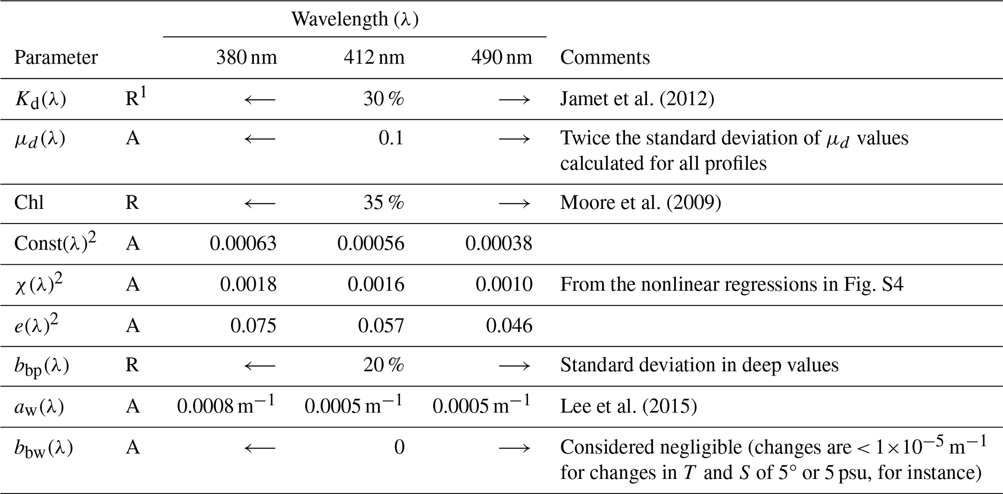
¹ R or A in the second column indicate either a relative or absolute uncertainty. ² See Eq. (5) for a_p vs. Chl.

3 Results

3.1 General a_y(λ) distributions

Histograms of retrieved a_y(λ) and corresponding spectral slopes are shown in Fig. 2. The mode values of a_y in the SO are 0.0261 m⁻¹ at 380 nm, 0.0194 m⁻¹ at 412 nm, and 0.0073 m⁻¹ at 490 nm. For the low-latitude waters, the corresponding values are 0.0239, 0.0139 and 0.0036 m⁻¹. Notably, only about 2 % of the a_y(380) retrievals in the SO are negative, compared with 4 % at 412 nm and 20 % at 490 nm. In the low-latitude waters, the respective percentages are 2 %, 6 % and 29 %. This is expected, as a_y(490) is significantly smaller than a_y(380) (due to the exponential decrease with wavelength) and because the method has larger uncertainty at 490 nm. Additionally, the spectral slope of a_y(λ), S (nm⁻¹), was calculated for the 3 possible wavelength pairs, and as the average of the a_y spectral dependence between 380 and 490 nm and between 412 and 490 nm. The mode value of S in the SO is 0.009 and 0.015 nm⁻¹ for the low-latitude waters. The latter is close to the value of 0.014 nm⁻¹ reported by Bricaud et al. (1981).

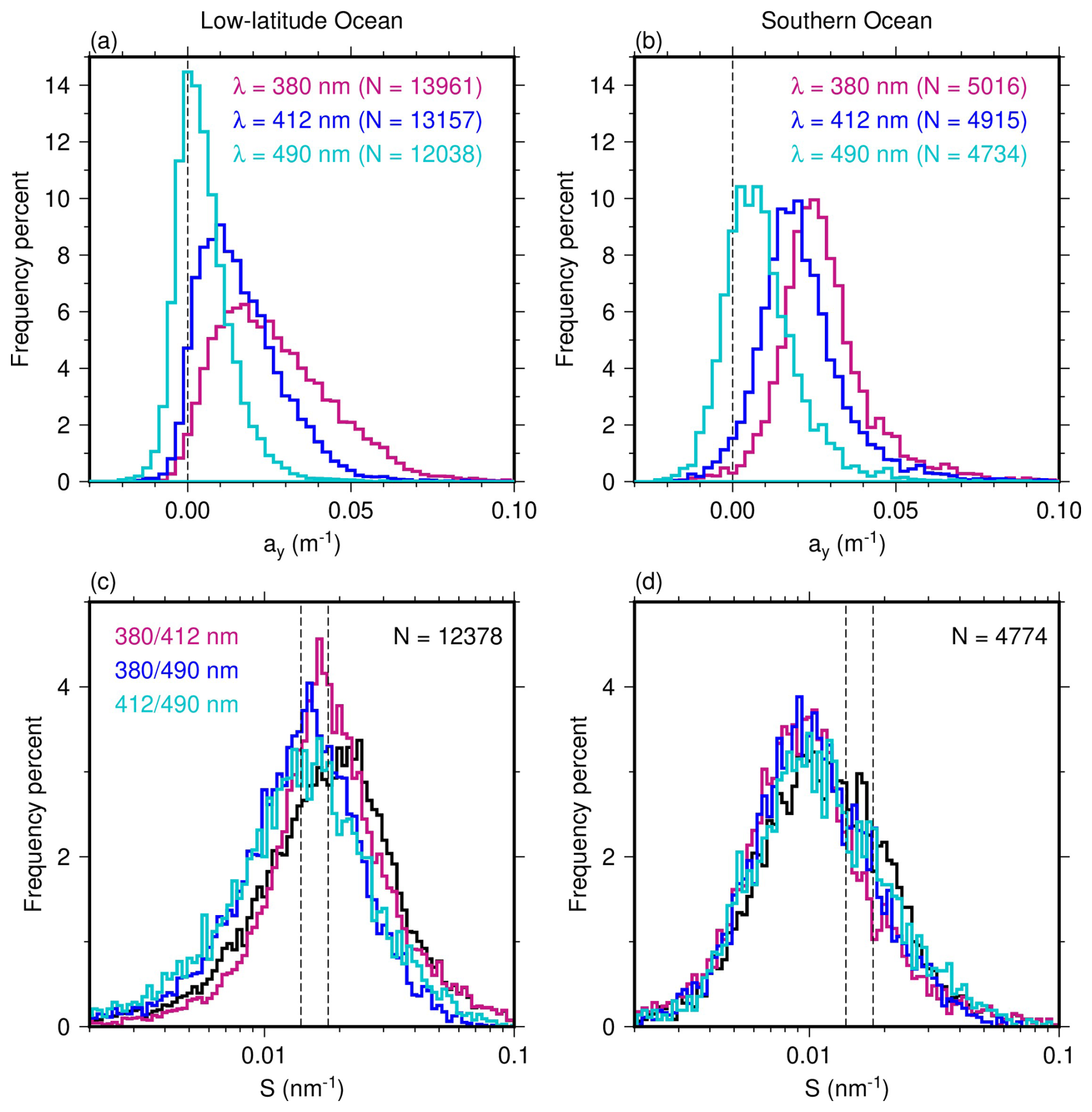
Figure 2 Distributions of a_y as derived from the BGC-Argo data at the three wavelengths indicated and for the low-latitude Ocean (a) and the SO (b). The corresponding spectral slopes are displayed in (c) and (d), both when separately calculated for the three wavelength pairs indicated and when these three estimates are averaged (black line). The dashed lines in (c) and (d) are the S values proposed by Bricaud et al. (1981) (0.014 nm⁻¹) and those used by Morel and Gentili (2009) (0.018 nm⁻¹).

The latitudinal distributions of the average values of a_y(380), the spectral slope of a_y (average value shown on Fig. 2c, d) and Chl, calculated from all data available in 2° latitude belts, are illustrated in Fig. 3. Generally, a_y(380) fluctuates between about 0.01 and 0.04 m⁻¹ south of 30° S, which is larger than the range observed in low-latitude waters (30° S–30° N), where values around 0.01 m⁻¹ are quite frequent. This is consistent with the global a_y distribution that can be derived from Chl by Morel and Gentili (2009) (gold dots; hereafter referred to as MG09), except south of about 40° S where the values we derived here are lower; this latitudinal band is also a band of very low continent to ocean ratio. Larger values are observed north of 30° N with the increase of Chl towards northern latitudes. The largest spectral slopes are observed in subtropical regions around 30° S and 30° N and around 60° S. The lowest values are in the equatorial region and around 45° S and 45° N. These distributions vary little seasonally (not shown). Isolated higher values around 27° N are from two floats deployed in the northern Red Sea.

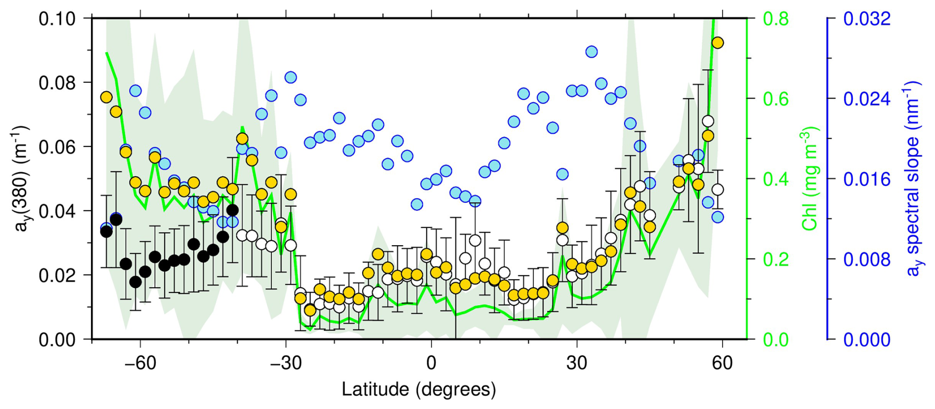
Figure 3 Zonal averages and standard deviation of a_y(380) for 2° latitude bands, calculated across our entire data set (open symbols for latitudes > 40° S and black symbols for latitudes < 40° S). The gold symbols are the a_y(380) estimated from the MG09 relationship for the average Chl values (green curve, with the standard deviation shown as the green shade). The spectral slope of a_y is also displayed (blue symbols; second scale on the right).

3.2 K_bio(λ) vs. Chl relationships

The K_d(λ) retrievals underpin the results shown in Figs. 2 and 3. Therefore, we assessed whether these retrievals were consistent with bio-optical relationships previously established for the low-latitude oceans under the form of the K_bio vs. Chl relationship, where K_bio is K_d−K_w, representing the contributions of all non-water components. The relationships for the low-latitude oceans are displayed in Fig. 4a, b, c, along with the MM01 model. The χ coefficients and the exponents of the K_bio vs. Chl relationships are within 15 % of those from MM01 at 380 and 412 nm and differ by about 45 % at 490 nm. The r² are accordingly decreasing from 0.5 at 380 to 0.33 at 490 nm. The slopes (exponents) of our relationships are lower than those from MM01. Despite these differences, these results show that the method used here can derive an overall consistent picture of the K_bio vs. Chl relationship for areas where it is well established. It is therefore supporting its use in the SO, where no such reference exists. Note that we cannot statistically assess the similarity between our relationships and MM01 because the data set that was used to derive the latter is no longer available.

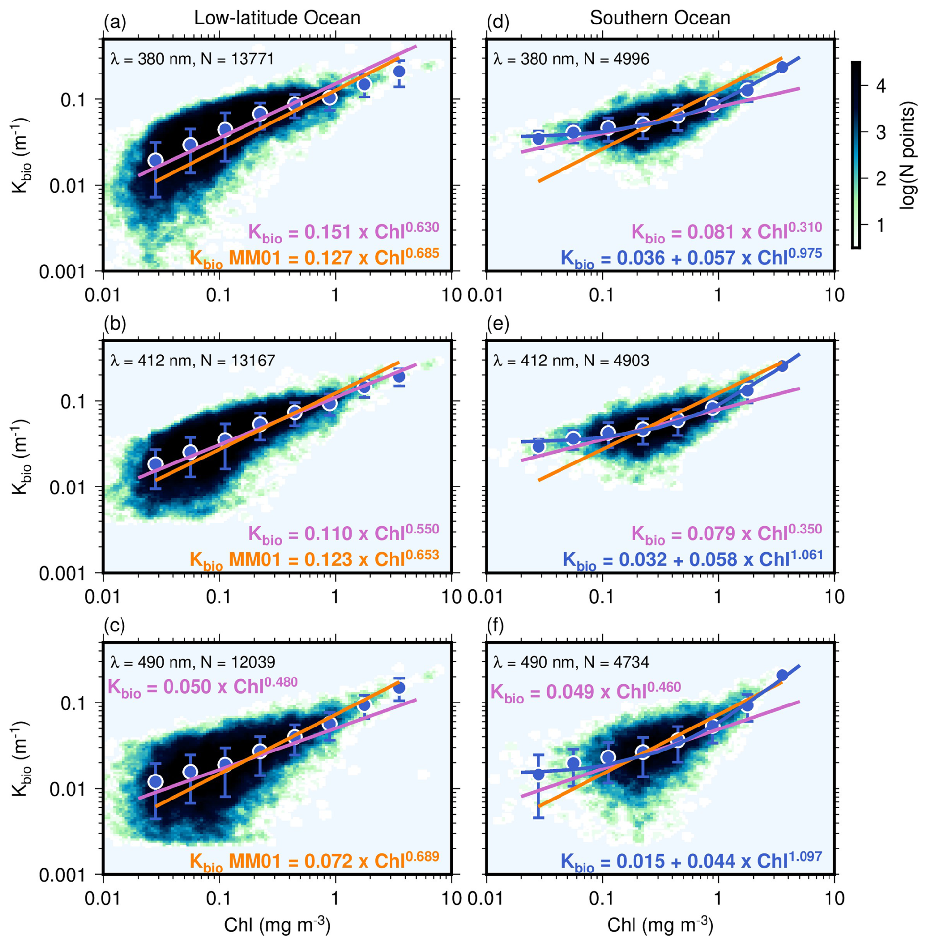
Figure 4 Non-water diffuse attenuation coefficient for downward irradiance (K_bio) for the three wavelengths indicated in the panels for the low-latitude oceans (left) and the SO (right) data sets. The blue-coloured density plots (scale on the top right) are built from all data obtained from individual float profiles. The large blue dots circled in white and vertical bars are average values and their standard deviation calculated over logarithmically equal Chl intervals. The purple and dark blue solid lines are a linear and a non-linear fits to all data points (log-transformed data; equations provided on each panel). The orange line for both the low-latitude oceans and the SO are for the Morel and Maritorena (2001) model (reported on the left panels as the “K_bio MM01” equation).

The results of the SO are displayed in Fig. 4d,e,f. Here the Chl range is smaller than in the low-latitude data set, spanning from about 0.05 mg m⁻³ (very few points below this value) to 3 mg m⁻³. The K_bio(λ) values do not follow the same decreasing trend as for the low-latitude oceans in the low Chl range (< 0.2 mg m⁻³). The MM01 relationships seem to fit our data quite well for Chl > ∼ 0.5 mg m⁻³. They do not match the data at lower Chl values, and the fit using a function of the form K_bio(λ)=χChl^e as in MM01 also fails to capture the curvature in this range. A better fit is obtained with a formulation similar to the one used for a_p (Eq. 5), displayed as the white curves in Fig. 4d, e, f, showing a low dependence of K_d on Chl below Chl ∼ 0.2 mg Chl m⁻³. The slopes of the linear fits (on log-transformed data) for the low-latitude waters are statistically different from those of the SO data (t-test) at 380 and 412 nm but are not at 490 nm, where uncertainties in deriving a_y are larger.

3.3 a_y(λ) vs. Chl relationships

Similarly to K_bio(λ), we analyzed a_y as a function of Chl (Fig. 5). The relationships we obtained for the low-latitude areas are similar to those proposed by Morel and Gentili (2009), except for λ= 490 nm, where the dispersion of the a_y values is the largest, as expected from the methodology. Therefore, results at this wavelength must be considered with caution. Given that MG09 was originally developed at 400 nm and subsequently extended to other wavelengths using a spectral slope of 0.018 nm⁻¹, and our a_y at 412 nm is the closest match to 400 nm, here we compare it with MG09 at 412 nm to minimize the potential discrepancy that might occur from wavelength conversions involving larger spectral distance. In low-latitude waters, MG09 generally aligns with our predicted a_y(412) vs. Chl relationship, apart from Chl > 3.0 mg m⁻³, where additional data is required for further assessment. This further confirms the validity of our float-based inversion approach. As previously said for K_bio, we cannot statistically assess the similarity between our relationships and MG09 because we do not have the data set that was used to derive the latter.

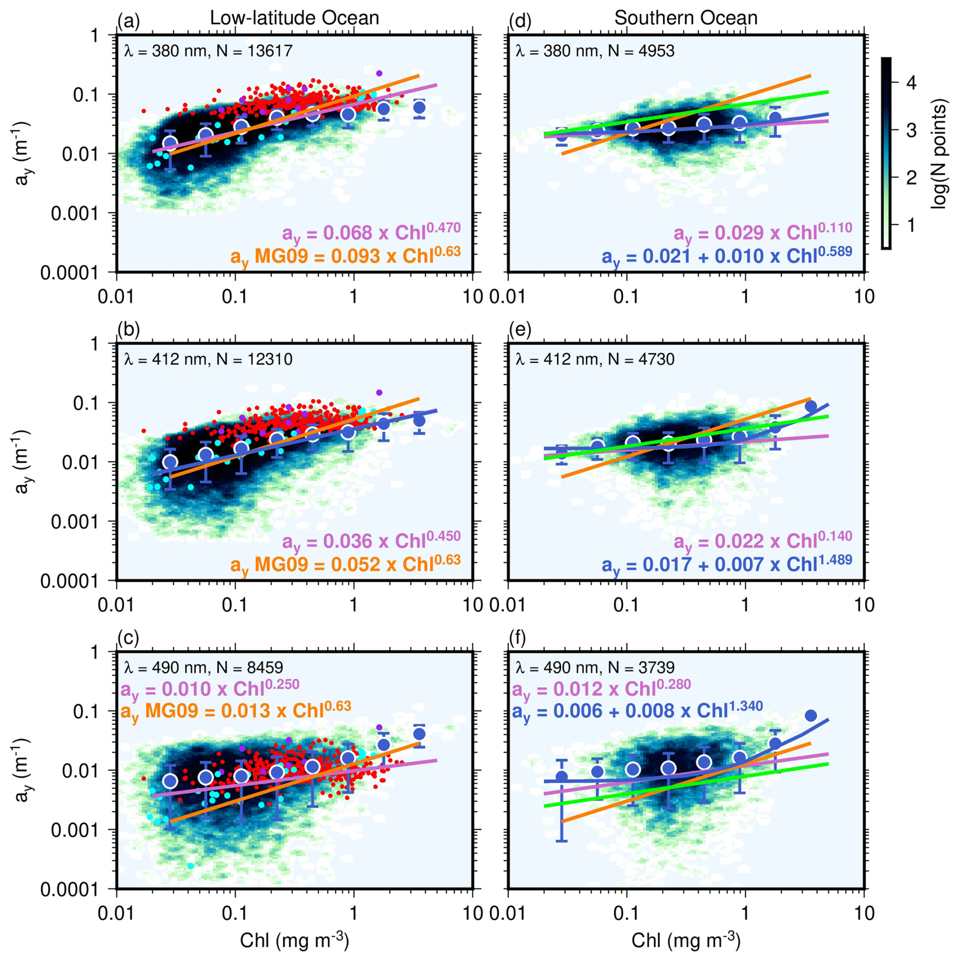
Figure 5 CDOM absorption (a_y) for the three wavelengths indicated and for the low-latitude waters (left) and the SO (right) data sets. The blue-coloured density plots (scale on the top right) are built from all data obtained from individual float profiles. The large blue dots circled in white and vertical bars are average values and their standard deviation calculated over logarithmically equal Chl intervals. The purple and dark blue curves are a linear and non-linear fits to all data points (log-transformed data), the orange lines are from the Morel and Gentili (2009) model, whose equations are also reported as “a_y MG09”. The green lines are from Reynolds et al. (2001). In panels (a), (b) and (c), the coloured dots are in situ measurements of a_y from the BOUSSOLE site in the Mediterranean Sea (red dots), the BIOSOPE research voyage in the Southeast Pacific gyre (turquoise), and the NOMAD data set (purple) that covers various oceans.

The BOUSSOLE data sit on the upper part of the data cloud and the BIOSOPE data rather in the middle of it, with some low values for low Chl, which is consistent with what has already been shown for the Mediterranean Sea and the Southeast pacific gyre (Morel et al., 2007c). The NOMAD data are also on the high range. This consistency of the derived a_y with field measurements further validates the approach.

In the SO (Fig. 5d, e, f), a_y does not vary much across the whole Chl range, with slopes of the a_y vs. Chl relationships much lower than those of the low-latitude data set and the MG09 model (equations reported on each panel of Fig. 5). The regression coefficient of the relationship at 380 nm in low-latitude waters is 0.26, whereas for the SO it is less than 0.1 across all wavelengths. Confidence intervals and a t-test show that all slopes (the B exponent in the A × Chl^B relationships) are statistically different from zero, showing that the dependence of a_y on Chl still exist but is weak for the SO.

Reynolds et al. (2001) have reported an a_y vs. Chl relationship for the Ross Sea and Antarctic Polar Front Zone, expressed as a_y(400)=0.046 Chl^0.298 ($r^{\mathrm{2}}=\mathrm{0.55},N=\mathrm{55})$. When extrapolated to other wavelengths using the spectral slope they got from their data set (S=0.0195 nm⁻¹), the slopes of these a_y vs. Chl relationships sit between those of our relationships and those of MG09 (Fig. 5d, e, f).

3.4 Distribution of a_y anomalies.

Figure 5 shows that the a_y vs. Chl relationship established for low-latitude oceans do not match the SO data. We did not find coherent spatial patterns of the difference between the a_y derived here in the SO and the values calculated from Chl following MG09.

These differences, hereafter referred to as anomalies (with respect to the model), however display a seasonal pattern (Fig. 6a; black dots), with small differences during austral winter (June–September) and large negative anomalies in summer. When only clear waters are considered (Chl < 0.2 mg m⁻³; blue dots) the anomalies are small and do not exhibit the same seasonal pattern. A seasonal change is also observed in the a_y spectral slope (orange dots on Fig. 6), with higher values in summer that are close to the average values often considered for the low-latitude oceans (0.014 nm⁻¹; Bricaud et al., 1981), and lower average values in winter, down to about 0.009 nm⁻¹. These anomalies are plotted as a function of the MLD in Fig. 6b, showing the largest negative values for MLDs between about 50 and 100 m. These MLD values are typical of summer months, as shown in the insert of Fig. 6b (December to March/April).

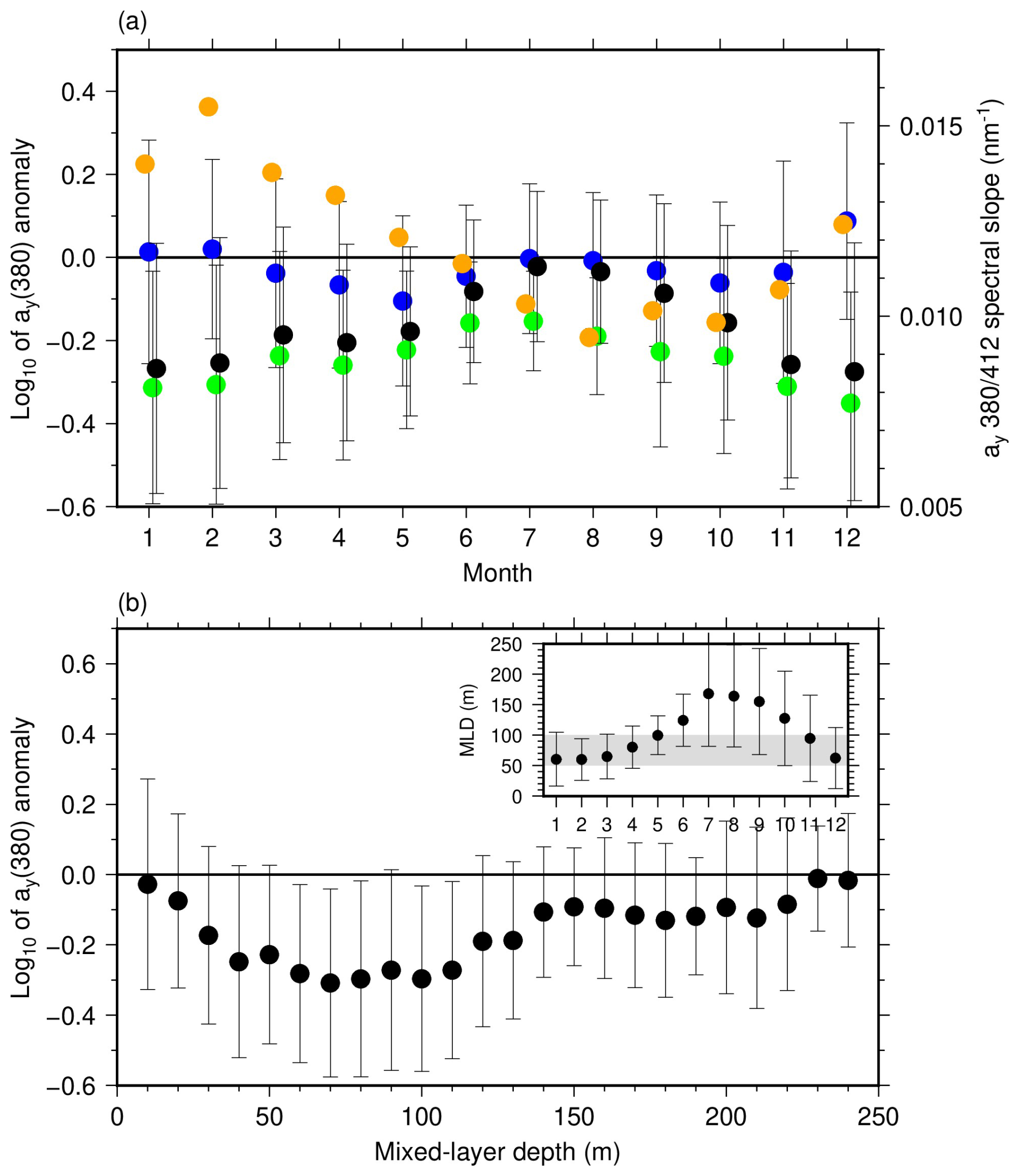
Figure 6 (a) Monthly average values (dots) and standard deviations (vertical bars) of a_y anomalies as a function of month of year (left scale) for the SO data. The anomalies are expressed as the decimal logarithm of the ratio of observed to modelled a_y, where the modelled values are from Morel and Gentili (2009). The blue dots are for Chl < 0.2 mg m⁻³, the green dots for Chl above that threshold, and the black dots for all data. The orange dots are the monthly average values of the spectral slopes calculated between 380 and 412 nm (right scale). (b) The same anomalies as in (a) plotted as a function of the mixed-layer depth (MLD), with the insert showing the seasonal course of the MLD in our data set. The greyed area shows MLD values between 50 and 100 m, corresponding to the largest negative anomalies.

3.5 Relative contributions of the absorption and scattering terms and uncertainties of a_y estimates

The relative contributions of the five terms into which $\left[\right(K_d{\mathit{\mu }}_d)/\mathrm{1.0395}]$ is split (Eq. 4) were derived for the entire data set (Fig. 7a, b) and also calculated from bio-optical models (Fig. 7c). The larger the contribution of a_y the lower the sensitivity of its derivation through Eq. (4) will be to the values of the other four terms. The first observation is that a_y shows the largest relative contribution at 380 nm, often around 50 % for both the low-latitude and SO waters. As expected from the spectral dependence of a_y, the contribution is smaller for longer wavelengths, with percentages ranging from about 30 % to 50 % at 412 nm and from about 20 % to 30 % at 490 nm (see Fig. S5). The large relative contributions for the shortest wavelengths creates favorable conditions to operate Eq. (4).

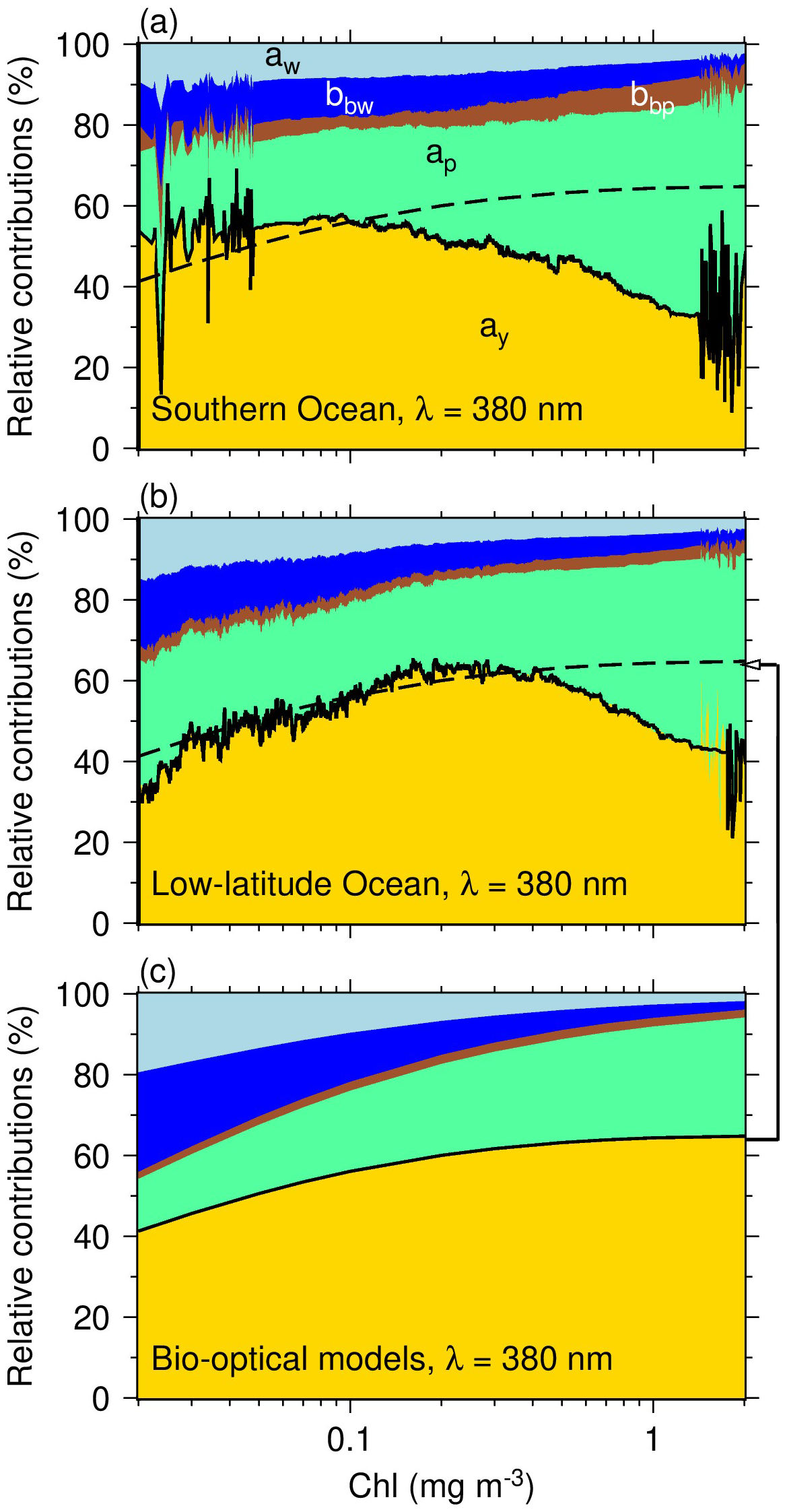
Figure 7 Relative contributions of a_w (light blue), b_bw (blue), b_bp (brown), a_p (green) and a_y (gold) to $\frac{K_{\mathrm{d}}\left(\mathit{\lambda }\right){\mathit{\mu }}_d\left(\mathit{\lambda }\right)}{\mathrm{1.0395}}$ (Eq. 4) at λ= 380 nm, as a function of Chl. Panel (a) is for the SO, (b) is for the low-latitude Oceans, and (c) is when using Bricaud et al. (1998) to calculate a_p, MG09 for a_y, and MM01 for b_bp. The thick black line delineates the contribution of a_y(380) to the budget. This modelled relative contribution of a_y from panel (c) is reproduced in (a) and (b) as a dashed line. The increased noise in that curve for Chl < 0.03 mg m⁻³ and Chl > ∼ 1.5 mg m⁻³ arises from the low numbers of retrievals in these ranges.

Figure 7 also shows that the relative importance of absorption by particulate matter for both the SO and the low-latitude oceans remains relatively constant around 20 %–25 % for Chl < ∼ 0.2 mg m⁻³, and then increases beyond this concentration to reach about 50 %. This is constrained here by the use of the Bricaud et al. (1998) parameterization and our Eq. (5).

The relative contribution of a_y(380) for the low-latitude oceans increases from about 30 % for the lowest Chl to ∼ 60 % for Chl ∼ 0.25 mg m⁻³, similarly to what bio-optical models predict (dashed line on Fig. 7b). However, beyond Chl ∼ 0.5 mg m⁻³ the model and the observations evolve in opposite ways, the latter showing the relative contribution of CDOM decreasing to 40 %. For the SO waters, this contribution is steadily around 55 % for Chl < ∼ 0.2 mg m⁻³, which is larger than for the low-latitude waters, and then regularly decreases down to 30 % when Chl is ∼ 2 mg m⁻³. These changes for SO waters do not match what the bio-optical models predict over the entire range of Chl here considered.

There are several sources of uncertainty when deriving a_y from K_d using Eq. (4) without having concomitant measurements of the various parameters of the equation such as a_p. These uncertainties were assessed as described in section 2.6. At 380 nm in the SO, there is little sensitivity of the overall distribution of the derived a_y to different approaches to obtain K_d (Fig. 8a), μ_d (Fig. 8b) and a_p (Fig. 8c).

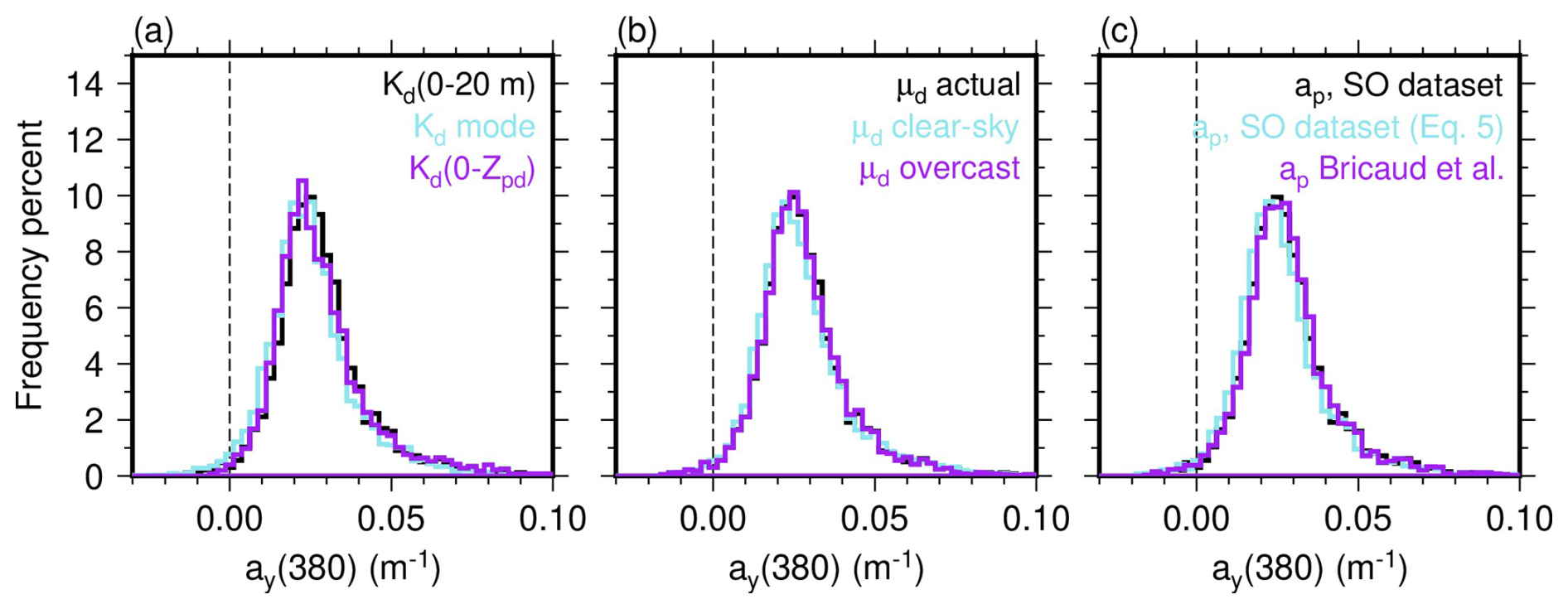
Figure 8 Distribution of a_y(380) resulting from (a) three approaches to obtain K_d from E_d(z,380), (b) whether the distinction between clear and cloudy sky is applied when calculating μ_d or ignored and then μ_d being forced to either its clear sky or overcast sky value, and (c) using the three different a_p vs. Chl relationships displayed in Fig. S4. Data for the SO only.

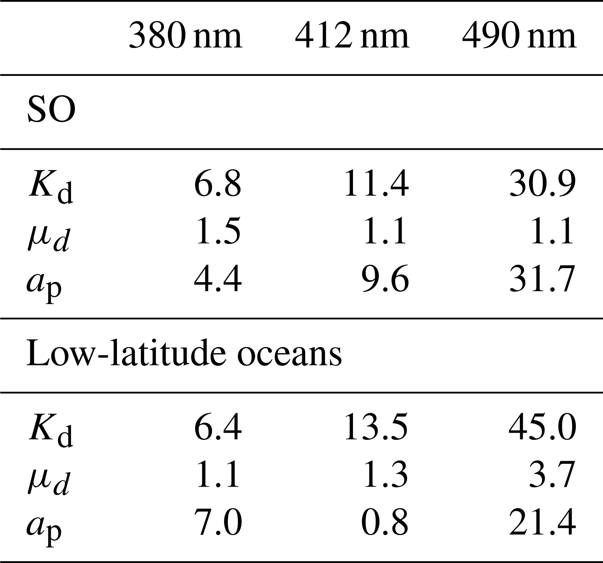
Associated statistics are given in Table 2. As expected, uncertainties in K_d contribute the most to differences in the retrieved a_y, followed by a_p and μ_d. Results are similar at 412 and 490 nm and for the low-latitude waters, except for a_p at 412 nm in low-latitude oceans. They show increasing sensitivity to the three parameters with increasing wavelength.

Table 2 Average dispersion (%) of the mean a_y values with respect to their average for the three instances of each sensitivity study and the three wavelengths. For each parameter (K_d, μ_d and a_y), the dispersion is calculated as the mean absolute difference among average values for this parameter for each of the three sensitivity studies, divided by the average value calculated for the three studies together.

The results of the Monte Carlo analysis applied to the SO data set are displayed in Fig. 9, as the distribution of the coefficient of variation (CV, defined as 100 × standard deviation divided by the mean) of a_y(λ) values obtained for each individual estimate of K_d(λ). Each CV results from 10 000 runs of Eq. (4) using randomly picked errors on the individual terms of the equation (see methods). The modes of the histograms show that an uncertainty around 18 % can be generally expected for λ= 380 and 412 nm, and 25 % for λ= 490 nm. Cumulative curves (not shown) indicate that 85 % of uncertainties are lower than 20 % for λ= 380 nm, 60 % at 412 nm and 20 % at 490 nm, reemphasizing that the band at 490 nm is far less adapted to deriving a_y from Eq. (4) than the two other bands.

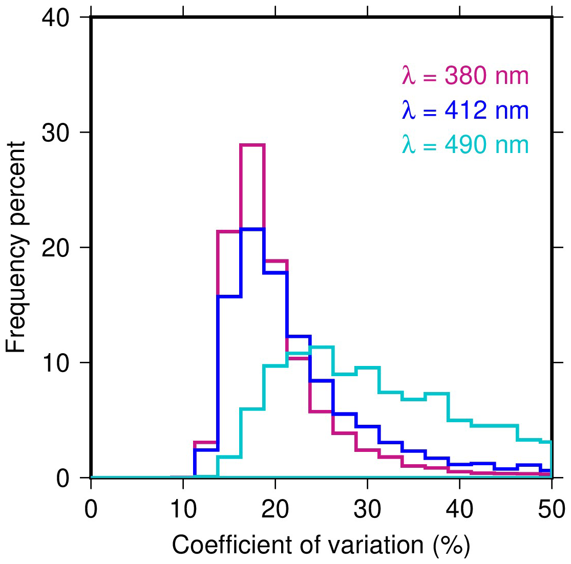
Figure 9 Distribution of the coefficient of variation of a_y(λ) values obtained by running the Monte Carlo analysis on each of the individual estimates of K_d(λ).

4 Discussion

4.1 Uncertainties of a_y estimates

Since the estimation of a_y is based on a series of empirical and semi-analytical bio-optical relationships, it is subject to several sources of uncertainty. The individual sensitivity analyses (Fig. 8, Table 2) and the Monte Carlo analysis (Fig. 9) have shown that uncertainties on a_y are non negligible. Nevertheless, meaningful a_y vs. Chl relationships could be derived thanks to the large size and dynamic range of the float data set, and to the normal distribution of errors. Our uncertainty assessment did not consider possible systematic large biases in the initial K_d values. The results in Fig. 4, including the comparison with MM01, did not show evidence that such biases are present.

The adjustment we applied to the Chl values for the low-latitude areas is another source of uncertainty. When it is not performed, the slope of the a_y vs. Chl changes slightly (e.g., from 0.57 to 0.45 at λ= 412 nm), yet the observation that a_y in the SO does not vary with Chl as strongly as it does in the low-latitude areas still holds.

Considering the uncertainty on the Fluorescence-to-Chl conversion factor, we tested the impact of using the Sauzède et al. (2025) lookup table that provides a global 1-degree resolution map of the fluorescence-to-Chl ratio instead of using constant factors (3.79 is the SO and 2 elsewhere). In this sensitivity study, the BGC-Argo Chl data were re-multiplied by a factor of 2 and divided by the fluorescence-to-Chl ratio from the lookup table corresponding to the location of the float. The results in terms of global distributions (Figs. 2 and 3) and relationships to Chl were not appreciably modified.We opted not to use this lookup table, however, because it is based on Chl values derived from K_d(490) using a bio-optical model similar to MM01, which has been shown here not suitable for the SO.

The way we calculated the a_y spectral slopes is sensitive to errors in individual a_y values. We nevertheless obtained average values for the low-latitude data set (Figs. 2c and 3) that are close to those generally considered as representative of open-ocean conditions (Bricaud et al., 1981; Morel and Gentili, 2009). The range of values shown in the general distribution of this slope (from about 0.008 to 0.024 nm⁻¹; Fig. 3) is also consistent with previous studies (e.g., Wei et al., 2016; Aurin et al., 2018). Higher values in subtropical areas are expected because of the high impact of photobleaching in stratified waters.

4.2 Comparison with bio-optical models and implication on ocean colour remote sensing

Differences in a_y vs. Chl relationships between the SO and low-latitude waters may lead to biases when using standard ocean color algorithms to estimate Chl in the SO. Figure 7 shows that the MG09 and Bricaud et al. (1998) bio-optical models predict an overall relative contribution of [a_y+a_p] to $K_{\mathrm{d}}\left(\mathit{\lambda }\right){\mathit{\mu }}_d\left(\mathit{\lambda }\right)/\mathrm{1.0395}$ (the yellow plus green areas combined) that is close to what we observe for both the SO and the low-latitude waters, except for low Chl values where the contribution from the models (∼ 55 %) is lower than from the observations (∼ 70 %). These differences do not seem high with respect to the method uncertainties. However, the relative contributions of a_y and a_p do not follow the modeled pattern. For low-latitude waters, the divergence starts when Chl > ∼ 0.5 mg m⁻³, with the relative contribution of a_y then decreasing significantly towards larger Chl. Below this Chl threshold the predictions and observations are similar. For the SO, the relative contribution of a_y is slightly larger than what the models predict for Chl < ∼ 0.15 mg m⁻³. Then the divergence with the model when Chl increases is much larger than what it is for the low-latitude areas.

These observations have implication on the quantification of Chl through satellite algorithms such as the OC4Me (Morel et al., 2007a), which is based on the MM01 bio-optical model, itself consistent with MG09 and Bricaud et al. (1998) used here (Morel, 2009). These bio-optical models underlying OC4Me assume a larger contribution of a_y than it is shown here for Chl values > ∼ 0.5 mg m⁻³, which could lead to underestimation of Chl in that range when current satellite algorithms are used. If applied to the SO, the algorithm will underestimate even more the large Chl values (the actual relative contribution of a_y being even smaller), yet it will overestimate low Chl values, in this case because the assumed contribution of a_y is lower than it actually is. These expected Chl over- or underestimations are actually what several validation studies have shown, as outlined in the introduction of this study (see also Dierssen and Smith, 2000).

4.3 Possible reasons for the different contribution of a_y in the SO as compared to low-latitude waters

Multiple factors can contribute to the discrepancy in a_y contributions between the SO and low-latitude waters, including differences in source inputs, as well as variations in the corresponding physical and biological processes. Due to the lack of terrestrial input, CDOM in the SO mainly derives from local sources, through in situ biologically-mediated production and consumption in the euphotic zone and redistribution via horizontal and vertical circulation. The redistribution is driven by physical processes such as winter seasonal mixing, subductions, upwelling and storms that can either bring deep CDOM-rich waters to the surface ocean or on the contrary dilute CDOM through mixing of surface waters with CDOM-poor waters (Nelson and Siegel, 2013; Mannino et al., 2014). Among these factors, the deep winter mixing plays a critical controlling role on CDOM dynamics by vertically homogenizing the water column and entraining CDOM-rich deep waters into the surface layer, thereby resetting the upper-ocean CDOM inventory each year. This deep mixing replenishes relatively refractory CDOM at the surface, counteracts cumulative summer photobleaching and microbial alteration, and establishes a consistent winter baseline for CDOM concentration and optical properties. By simultaneously resupplying nutrients that fuel the spring phytoplankton bloom, the winter mixed layer also indirectly regulates subsequent biological CDOM production. As a result, the depth and intensity of winter mixing strongly govern the seasonal amplitude, optical signature, and interannual variability of the CDOM pool in the SO.

The SO is structured by a succession of oceanic fronts that tend to isolate water masses (Park et al., 2019), experiences seasonal sea ice melt that releases organic matter in surface waters (Ortega-Retuerta et al., 2010a; Norman et al., 2011), and is home of pronounced vertical mixing (Olbers and Visbeck, 2005; Hillenbrand and Cortese, 2006). These characteristics create highly heterogeneous environments that influence the sources, transformations, and distribution of CDOM. In addition, the phytoplankton communities in the SO exhibit distinct physiological adaptations to the extreme light-limited conditions, which likely alter their production and release of CDOM compared to those in more illuminated waters (Strzepek et al., 2019). Collectively, these factors introduce substantial variability into a_y dynamics and apparently weaken its direct coupling with Chl, making it difficult to predict a_y from Chl in these high-latitude waters.

The local production is related to a wide range of biological processes including viral lysis, bacterial degradation, phytoplankton excretion and zooplankton grazing (Bricaud et al., 1981; Nelson et al., 1998; Nelson and Siegel, 2002; Siegel et al., 2002; Matsuoka et al., 2013; Bonelli et al., 2021). Loss mechanisms also determine the CDOM balance, including microbial consumption and photooxidation (Siegel et al., 2002; Nelson et al., 2007). Photobleaching is inefficient in winter due to the low incoming irradiation (Fichot et al., 2023). What Fig. 6 shows, however, is that photobleaching is likely significant in summer when the depth of the mixed layer is less than about 100 m and surface irradiance can be as high as it is in the equatorial belt (Campbell and Aarup, 1989). Photobleaching is expected to lead to an increase of the spectral slope of CDOM absorption (e.g., D'Sa and Kim, 2017). This increase is indeed observed in Fig. 6 and must be compensated by an effective decrease of the DOM pool to lead to the observed negative a_y summer anomaly.

We do not further speculate about other possible causes of the differences we observe between the SO and the low-latitude oceans. Complementary data or model outputs would be needed in complement to what autonomous BGC-Argo floats alone can provide.

4.4 Are departures unique to the SO or do they apply to the whole temperate Southern Hemisphere?

Figure 3 highlighted that the difference between the standard bio-optical model and the estimated a_y depart from one another for latitudes higher than 30° S. As noted above, this latitude also corresponds to where the fractional land (to ocean) contribution decreases rapidly. Whether this reflects the reduced impact of land contribution to the CDOM pool or another feature of temperate SO waters is unknown (note the near absence of BGC-Argo floats equipped with radiometers in the Pacific sector of the SO). However, the departure observed here may point to a much larger region where current bio-optical relationships are distinct at least with respect to CDOM. We also note that the CDOM index derived by Morel and Gentili (2009) does not seem to match our measurements in this region as it suggests higher than average concentration. Overall, the CDOM index often provides high values at high Chl in temperate waters, which fit with our observations in northern regions but not in the southern hemisphere.

4.5 Do Southern Ocean waters belong to Case 1 waters?

The concept of Case 1 vs. Case 2 waters (Morel and Prieur, 1977) has been instrumental by providing a global and consistent framework to quantitatively interpret satellite ocean colour observations. The concept is based on the observation that biological matter that drives bio-optical properties and hence ocean colour covaries with phytoplankton in open ocean waters, classified as Case 1 waters. This covariation only emerges, however, when a large dynamic range is considered, e.g., by pooling together data from various trophic levels and oceans. When the dynamic range is small, the correlation generally vanishes. In Case 1 waters, Chl can be used as a single index of changes in ocean colour, which does not mean that it is the sole responsible for changes. Assuming this general co-variability when deriving empirical chlorophyll algorithms, for instance, does not require separate consideration of how the components of the biological matter individually correlate with Chl (e.g., phytoplankton, detrital matter, CDOM) (Siegel et al., 2005). Variability in these relationships is a large source of uncertainty in the Chl retrieval from satellite ocean colour and has led to questioning whether the concept itself was useful (Mobley et al., 2004). When semi-analytical algorithms are developed, however, phytoplankton, non-algal particles and dissolved substances can vary independently from Chl (e.g., Bricaud et al., 1998; Lee et al., 2002; Maritorena et al., 2002; Siegel et al., 2005; Morel and Gentili, 2009).

The observation from Fig. 7 that the relative contribution of [a_y+a_p] to $K_{\mathrm{d}}\left(\mathit{\lambda }\right){\mathit{\mu }}_d\left(\mathit{\lambda }\right)/\mathrm{1.0395}$ predicted by the bio-optical models matches the observations supports the use of Chl to quantify the ocean colour signal following the Case 1 waters paradigm. While the CDOM concentration increases with Chl, this increase is not as strong as in other oceanic regions and the relative contribution starts decreasing at lower Chl (∼ 0.15 mg m⁻³ for the SO and 0.5 mg m⁻³ for low-latitude waters). As such while the SO would be expected to be “prototypical” case 1 waters with minimal influence of land and strong influence of biology, other factors – likely physical – have a strong impact on the weak relationship between Chl and CDOM. As a consequence, the relative contribution of CDOM to absorption in the SO, hence to the ocean colour signal, is larger than predicted by the bio-optical models here considered for Chl < ∼ 0.1 mg m⁻³ (55 % instead of 40 % for the lowest Chl) and much lower for Chl above that value (30 % instead of 60 % for Chl = 2 mg m⁻³). This is coherent with the observed underestimation of Chl in that range by current satellite ocean colour algorithms. Improved retrievals of Chl from satellite ocean colour observations over the SO will require revision of how CDOM absorption is parameterized.