Detection of tree stress from sub-daily sap flow variability

The terrestrial biosphere plays a critical role in regulating carbon and water fluxes. Rising global temperatures increase atmospheric dryness, which in turn raises atmospheric water demand on vegetation and places. Some plants regulate transpiration losses by closing stomata, at the cost of reduced carbon uptake. Quantifying stomatal regulation and detecting early onset of vegetation stress at large scales remains a challenge.

Sap flow in stems responds to water potential gradients between the roots and the atmosphere, and therefore provides a window into transpiration and stomatal regulation. Based on SAPFLUXNET measurements of sap flow across tropical, temperate and boreal biomes, we demonstrate how variations in the diurnal cycle of sap flow as a function of vapor pressure deficit (VPD) measurements can elucidate the different levels of plant hydraulic stress. We derive two metrics based on sub-daily responses of sap flow to VPD: the morning sensitivity, given by the slope of the bi-variate relationship, and the area of the diurnal sap flow – VPD curve. We find that seasonal variations in the morning slope are positively associated with top soil moisture (0–30 cm). The area of the diurnal cycle, characterizing the degree of daily hysteresis between sap flow and VPD, increases with sap flow downregulation before peak VPD and is sensitive to temperature and soil moisture variability at seasonal time scales.

While in situ sensors can provide continuous sap flow data, we aim to evaluate the potential to estimate descriptors of the diurnal cycle using temporally sparse data. In particular, as sap flow is connected to changes in water storage, which can be estimated using microwave remote sensing, we examine the degree to which the slope and area can be estimated for several acquisition strategies that vary in terms of the numbers of observations and acquisition times. We propose that sub-daily microwave observations, with at least three sub-daily overpasses could be used to characterize the sub-daily hysteresis and enable improved monitoring of tree hydraulic stress and, consequently, biosphere dynamics.

1 Introduction

Rising temperatures under global warming intensify the atmospheric demand for water (Vicente-Serrano et al., 2022a). This leads to reduced water availability, particularly in semi-arid regions, and heightens the risk of plant hydraulic stress or even hydraulic failure (Allen et al., 2015; Vicente-Serrano et al., 2022b). Climate change thus poses a significant threat to global vegetation health (Hartmann et al., 2022), raising serious concerns about ecosystem stability and the planet's ability to regulate climate (Bustamante et al., 2023).

Water plays a fundamental role in plant functioning, acting as a reactant in photosynthesis, regulating cell turgor and nutrient transport, and supporting evaporative cooling under hot temperatures. Water loss through evaporation in the stomata (transpiration) reduces leaf water potential, inducing the flow of sap from the soil through the root-stem-leaf continuum (sap flow, SF) and supporting the transport of nutrients through the xylem (Hammond et al., 2021). Regulation of stomatal aperture (stomatal conductance) allows plants to respond to changes in environmental conditions in order to preserve the continuity of the plant water column (Jarvis and McNaughton, 1986) and avoid embolism (Hammond et al., 2021).

Vegetation water dynamics provides critical insights into plant functioning and connect the carbon, water and energy cycles at time-scales from hours to decades. At longer time-scales (seasonal to interannual), variations in vegetation water content (VWC) typically reflect variations in vegetation biomass structure which are influenced by phenology, growth, natural disturbances and land-use (Konings et al., 2019). By contrast, vegetation water stress responses occur at time-scales from hours to months (Konings et al., 2019), with diurnal variations in vegetation water content and SF revealing signs of tree mortality several months before visual signs emerge (Hammond et al., 2021; Preisler et al., 2021).

Ecosystems have evolved varying strategies to cope with high atmospheric water demand and limited soil moisture availability. Maintaining high stomatal conductance through periods of high atmospheric water demand may increase gross carbon uptake and therefore promote faster growth, but increased rates of evapotranspiration may risk embolism and deplete water reserves if dry conditions persist (McDowell et al., 2022). Downregulation of transpiration through stomata reduces water loss, thus preserving water reserves, but also reduces the diffusion of CO₂ into the leaf, thus coming at the expense of reduced carbon uptake in the short term, and the availability of carbon for growth and plant maintenance, in the long run (Hammond et al., 2021). The outcome of these different strategies is complex and depends on multiple factors, such as drought characteristics, environmental factors, ecosystem memory and compounding effects (Cranko Page et al., 2022; Peltier and Ogle, 2023; Bastos et al., 2021) and biotic interactions (Seidl et al., 2017). Tracking the responses in vegetation water content and fluxes to changing atmospheric conditions is crucial for understanding the vitality of global ecosystems and assessing their potential risk of mortality (Preisler et al., 2021; Hammond et al., 2021; Landsberg et al., 2017; Rowland et al., 2015)

Diurnal fluctuations in VWC and SF reflect normal operating conditions of xylem water transport and are regulated by vegetation water storage, refilling and stomatal responses, which balance carbon uptake and transpiration-driven water loss (Jarvis and McNaughton, 1986). Plant water potential typically ranges from relatively high values at pre-dawn, when soil water is generally not limiting and incoming radiation is low, to low values during solar noon and afternoon, particularly on clear-sky days when light and evaporative demand are high. Healthy plants with sufficient soil water available can recharge overnight, when transpiration demand is low (Forster, 2014). Increasing transpiration through the morning decreases leaf water potential, which drives a corresponding increase in SF (Tyree and Ewers, 1991). Stomatal regulation may decouple transpiration, and consequently SF, from atmospheric water demand (Franks et al., 2017), giving rise to a characteristic diurnal hysteresis “loop” (Xu et al., 2022; Wan et al., 2023). In contrast, periods of prolonged drought can deplete root-zone soil moisture, reducing overnight recharge of vegetation water storage and lowering pre-dawn water content and plant water potential, leading to a certain level of stress (Davis and Mooney, 1986; Limousin et al., 2009, 2010b). Nighttime VWC values remain low if water is not sufficiently refilled, and stress effects are more pronounced around mid-day. Under extreme stress, embolism and tissue data can result in sap flux failure, resulting in dampened sub-daily SF variability, which can be used as an early sign of tree mortality (Preisler et al., 2021; Hammond et al., 2021). Variations in the sub-daily relationships between VWC, SF, and atmospheric vapour pressure deficit (VPD) therefore provide insight into plant water regulation strategies, vegetation responses to environmental stressors and, ultimately, health.

Currently, processes associated with plant functioning such as plant evapotranspiration and productivity are monitored at sub-daily temporal resolution in networks of sites such as FLUXNET (Pastorello et al., 2020), ICOS (ICOS RI, 2022), or SAPFLUXNET (Poyatos et al., 2021). However, these networks are relatively sparse and predominantly concentrated in North America and Europe (Pastorello et al., 2020; Poyatos et al., 2021). Remote-sensing plays a key role in large-scale and spatio-temporally consistent monitoring of plant water dynamics. Many studies have shown that radar observations are influenced by dynamics in VWC. A commonly used approach is to estimate VWC based on vegetation optical depth from spaceborne microwave sensors (e.g. Frappart et al., 2020; Zotta et al., 2024; Konings et al., 2021). However, current and planned microwave missions provide one snapshot every few days, observing “slow” ecosystem dynamics. They are adequate to observe inter- and intra-annual variations of above ground biomass (AGB), the slow response in water status over weeks and months, and to map (a-posteriori) biomass loss due to deforestation or mortality. This is, however, not sufficient to capture plant water dynamics associated with health and stress as discussed above.

Sub-daily synthetic aperture radar (SAR) observations have been proposed as a means for improved assessments of vegetation health and stress (e.g. Steele-Dunne et al., 2024; Matar et al., 2024). Dawn/dusk differences have been observed in spaceborne radar backscatter from vegetated areas and attributed to variations in water status (Steele-Dunne et al., 2012; Frolking et al., 2011; Friesen, 2008; Konings et al., 2017). Daily cycles obtained by aggregating Ku-band backscatter exhibit water loss/recharge patterns analogous to those illustrated in Fig. 1a (Paget et al., 2016; Van Emmerik et al., 2017; Konings et al., 2017; Prigent et al., 2022). Sub-daily variations in radar observables (backscattering coefficient, coherence, phase) have been measured using tower-based radars in a range of vegetation types and conditions (Ho Tong Minh et al., 2013; Hamadi et al., 2014; Ulander et al., 2019; Ulander and Monteith, 2022; Monteith and Ulander, 2022; Ouaadi et al., 2021; McDonald et al., 1990; Chakir et al., 2021; Vermunt et al., 2021, 2022; Khabbazan et al., 2022), with several of the more recent studies demonstrating the link to VWC using destructive sampling, and the link to SF using co-located in-situ sensors. Holtzman et al. (2023) have shown that increasing the number of observations from twice to four times a day could contribute to a large reduction in evapotranspiration and gross primary productivity estimated in a data-assimilation framework.

This study aims to contribute to the development of future sub-daily monitoring missions targeted at monitoring plant stress by providing insight into the number and timing of observations needed to characterize diurnal dynamics in VWC and SF as illustrated in Fig. 1. We hypothesize that certain characteristics of the sub-daily response of VWC and SF to VPD can help fingerprint periods and drivers of hydraulic strategies of vegetation, disentangle top-down (i.e. atmospheric demand) and bottom-up drivers (i.e. soil moisture supply) of hydraulic limitation and plant water use strategies (Fig. 1b–e). Since water transport and stomatal regulation are near-instantaneous responses to stress conditions (Choat et al., 2018), diurnal hydraulic hysteresis signatures potentially provide early-warning indicators that may significantly precede optically visible signs of vegetation decline (Preisler et al., 2021; Hammond et al., 2021). Our analysis is guided by two central research questions: (1) To what extent can plant responses to hydrometeorological stressors be characterized using descriptors of diurnal SF–VPD hysteresis? (2) How often, and at what times, would sparse observations be sufficient to estimate these descriptors?

In order to address these questions, we investigate the sub-daily variability in the SF–VPD relationship and its link to diverse hydrometeorological stressors, based on hourly SF measurements from the SAPFLUXNET database (Poyatos et al., 2021) at high temporal resolution (hourly) across a wide range of biomes. We then propose a reduced set of descriptors that can be derived from the diurnal hysteresis cycles, and that could be estimated using comparatively sparse sub-daily observations of VWC, or some proxy for it, from satellite remote sensing. We then examine the seasonal and interannual evolution of these descriptors at selected sites to understand how they vary in response to hydrometeorological conditions and particularly extremes. Finally, we compare several observation scenarios to investigate how well these metrics could be determined with sparser data from satellite remote sensing. We test the degree to which it is possible to capture the key characteristics of SF–VPD hysteresis with targeted sub-daily measurements using experiments characterizing hysteresis in SF with plausible data acquisition strategies, which is important for understanding the minimum requirements for observation frequency if observing sub-daily hydraulic dynamics with satellites. This would provide an opportunity for global monitoring of vegetation health and enable the early detection of vegetation stress before structural decline or canopy-level changes become detectable.

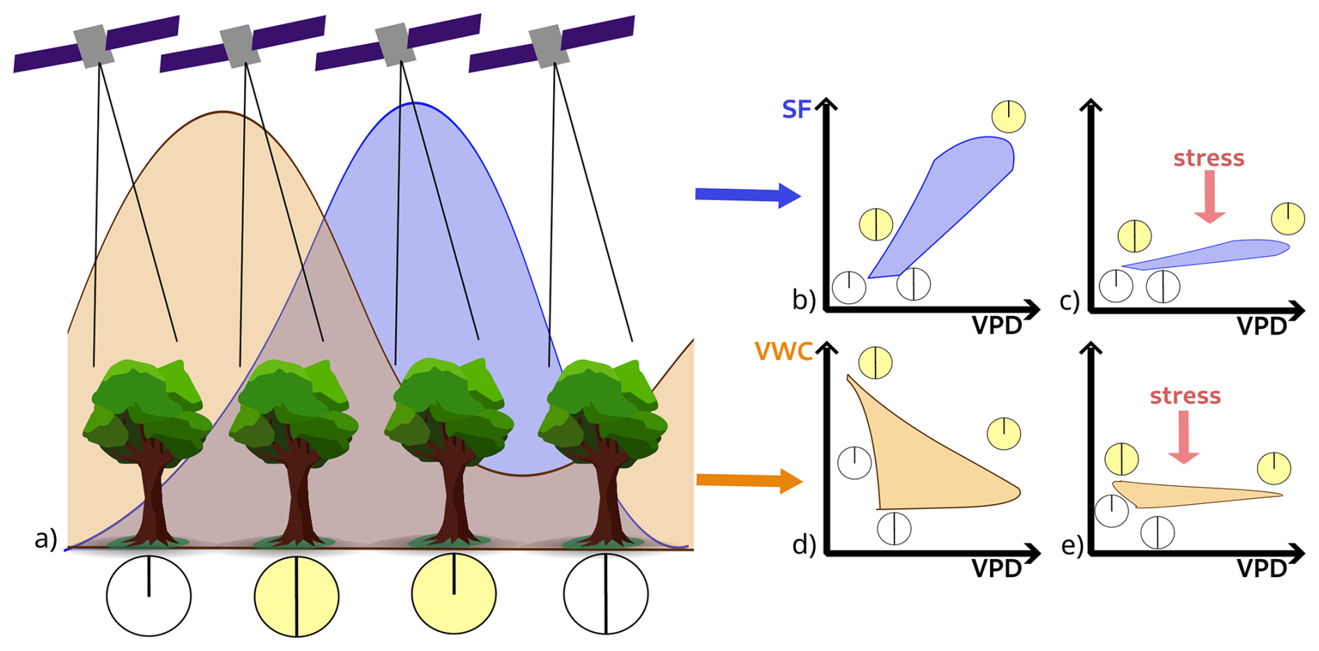
Figure 1 Conceptual representation of the diurnal variation in SF (blue) and VWC (orange). Hysteresis in the relationship between both quantities and vapor pressure deficit depends on environmental conditions and stress. It is hypothesized that characterizing this hysteresis with sub-daily observations at key times could provide insight into vegetation stress state and response. Panel (a) illustrates generalized diurnal cycles of SF (blue) and VWC (orange) and the critical times of the day at which a satellite could monitor VWC (midnight, 06:00 am, noon, 06:00 pm, from left to right). Panels (b)–(e) illustrate the hypothesised diurnal relationships of SF–VPD and VWC–VPD for average conditions (b, d) and for days marked by hydraulic stress (c, e). The circles in panels (b)–(e) show the times of the day represented in panel a). The different processes driving these responses are described in Sect. 1.

2 Material and Methods

2.1 Data and Study Sites

The SAPFLUXNET database (Poyatos et al., 2021) provides harmonized sap flow data from forest stands across 202 sites across the globe, covering the period 1995 to 2018. The sites are primarily located in Europe and the USA, with additional sites in Australia and South Africa, and a few in the tropics and high latitude regions. Each site offers half hourly or hourly time series, with an average duration of three years (Fig. 2).

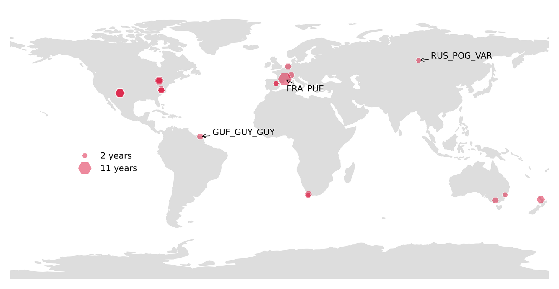
Figure 2 SAPFLUXNET sites where hourly SF and VPD, as well as air temperature and soil water content (SWC) have been measured at 80 % of days with a length greater than 12 hours for at least 2 years. The size of the hexagons indicates the number of years where time series of the sap flow data and the hydrometeorological drivers overlap. Three sites have been selected for more detailed comparison: the northernmost site (RUS_POG_VAR), the site closest to the equator (GUF_GUY_GUY) and the site with the longest timeseries of SF and VPD (FRA_PUE).

The database includes sap flow data expressed at different levels – plant, per sapwood area, or per leaf area – which are derived from heat dissipation, heat pulse and heat balance methods (Poyatos et al., 2021). Sensors are typically inserted into the sapwood at the trunk, providing a sap flux density, i.e., the rate of flow per unit sapwood area. Plant-level data can then be calculated by multiplying this density by the total sapwood area of the tree. To obtain leaf-level data, the plant-level sap flow is divided by the total leaf area, yielding an estimate of transpiration at the leaf scale. Not all site specific datasets include measurements for all three levels simultaneously. In this study, we selected only sites with plant-level data because it represents the largest scale of sap flow measurement, making it particularly useful for understanding whole-plant water dynamics (Poyatos et al., 2021).

In addition to sap flow (SF), the database includes observations of hydrometeorological variables such as photosynthetically active portion of incoming radiation (PAR, quantified as PPFD), 2 m surface air temperature (T_Air), precipitation (PRECIP), volumetric top soil moisture (0–30 cm, TSM) or vapour pressure deficit (VPD). With these ancillary variables, the SAPFLUXNET database allows the study of rapid tree responses to environmental conditions and helps to bridge the gap between ecosystem flux networks and remote sensing.

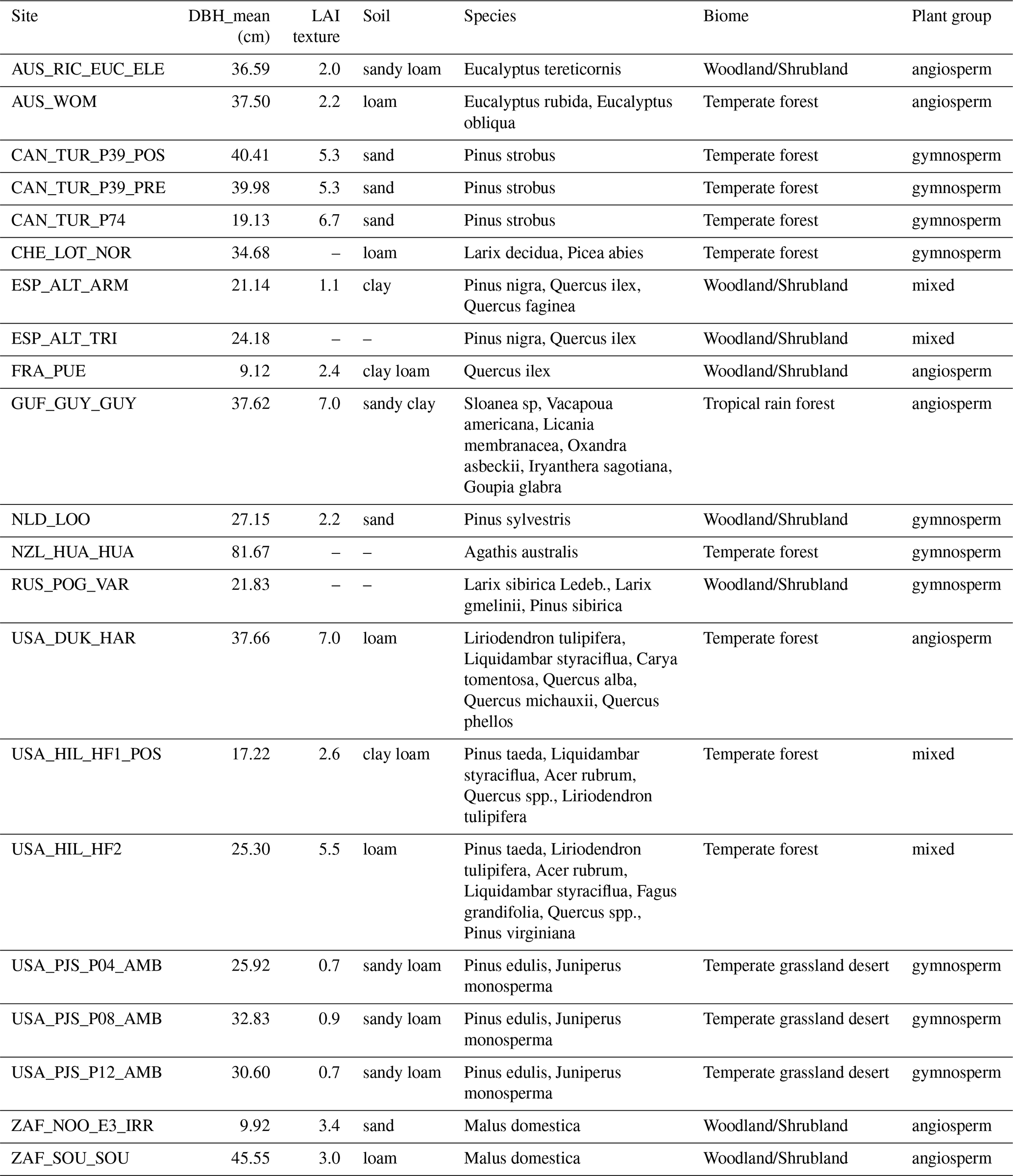
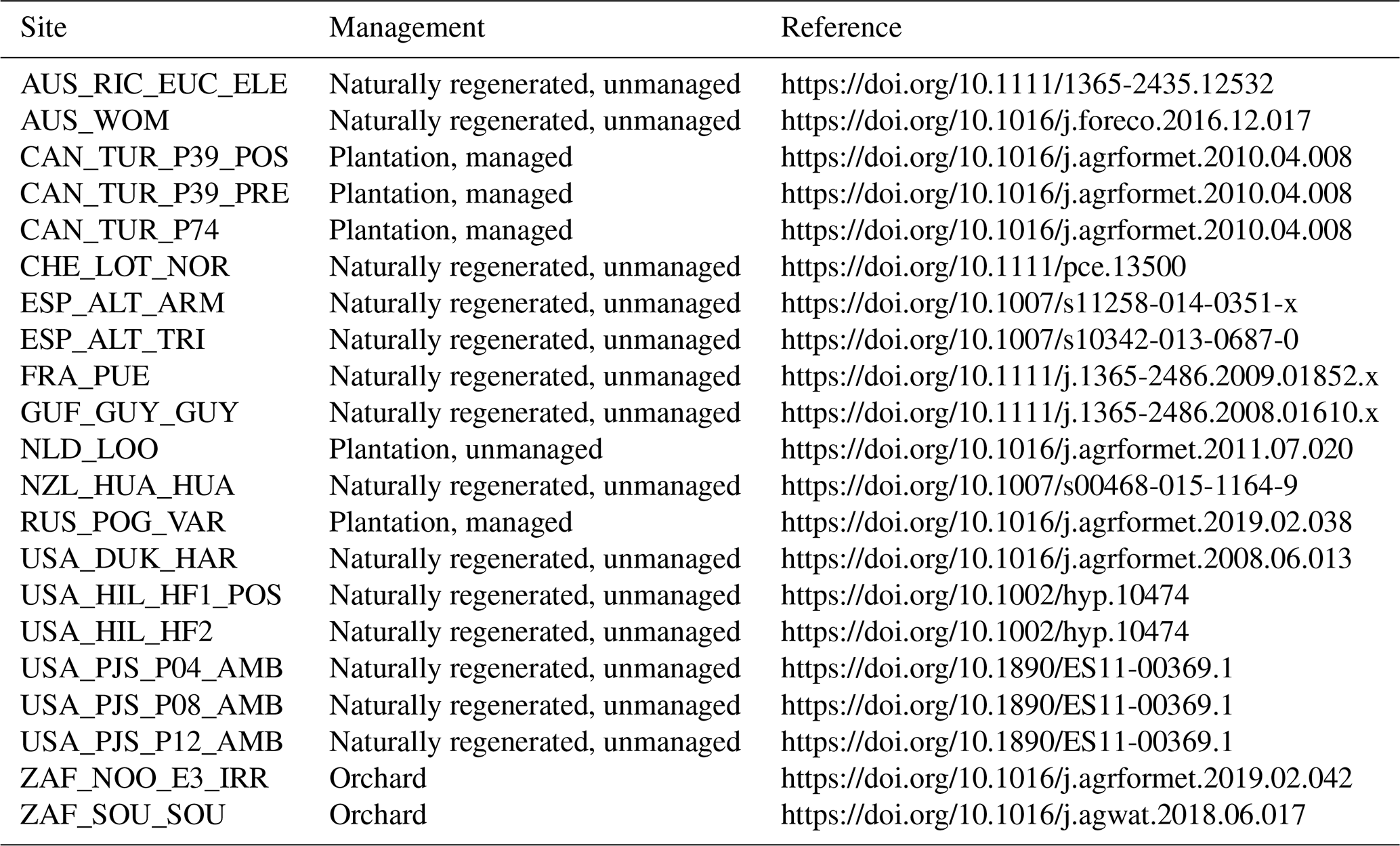
For the broader analysis of sub-daily sap flow dynamics and response to climatic drivers, we identified 15 unique sites where plant-level SF, as well as VPD, T_Air and TSM are available. Specifically, we selected sites where days with these data overlapped for at least 80 % of the growing season (defined based on day length >12 h and T_Air >5 °C) across two or more years. These 15 sites represent less than 15 % of all sites in the SAPFLUXNET database. Figure A1 shows how the mean temperature and precipitation varies across the 15 study sites. Furthermore, site-level information on mean Diameter at Breast Height, Leaf Area Index, soil texture, tree species, biome, plant group, treatment and site-specific publications are provided in Tables A1 and A2.

2.1.1 Focal sites

We selected three focal sites (highlighted in Fig. 2) representing a climate gradient from tropical humid regions, to hot semi-arid, and to cold permafrost environments (see Fig. A1) for a more detailed analysis. The selected sites are a mediterranean forest in Puéchabon, France (FRA_PUE), a humid tropical rainforest in French Guiana (GUF_GUY_GUY), and a forest-steppe in Pogorelsky Bor, Russia (RUS_POG_VAR). FRA_PUE was chosen for its exceptionally long time series of sap flow (SF) and vapor pressure deficit (VPD), providing a robust dataset for temporal analysis. GUF_GUY_GUY was selected as it is the site closest to the equator, representing a low-latitude humid tropical environment with a seasonal drought. RUS_POG_VAR represents the northernmost site, making it valuable for studying plant-water relations in cold, high-latitude conditions.

FRA_PUE is located 35 km northwest of Montpellier in southern France. This region is characterized by hot, sunny summers with low rainfall and strong winds, which are alternated by cool, wet winters, with rainfall primarily occurring between September and April (Limousin et al., 2009). The nearby Mediterranean Sea moderates the climate, resulting in an average temperature of 15.5 °C. However, rising temperatures due to climate change will increase drought severity in the region (Limousin et al., 2010a; Misson et al., 2011). The forest was historically managed as a coppice, meaning that all trees are approximately the same age and belong to the same species. The evergreen holm oaks (Quercus ilex), which reach a height of less than 7 m and a diameter of less than 13 cm, are situated on a plateau in a limestone karstic plateau. The soil is a shallow silty clay loam filling the cracks in the karst, with a volumetric fraction of rocks above 0.75. This leads to rapid infiltration in the subsoil and a reduced soil water holding capacity. The 25 studied holm oak trees exhibit a typical seasonal sap flow cycle, with reduced Gross Primary Production (GPP) and transpiration during periods of drought (Limousin et al., 2009; Cicuéndez et al., 2015; Allard et al., 2008). This site has the longest set of measurements in the SAPFLUXNET data, spanning 15 years (2000–2015) of which we can use 2003–2015, since VPD is not available earlier.

The GUF_GUY_GUY site is located in French Guyana on the east coast of the Amazon rainforest, near the equator. The northernmost part of the Guyana Plateau is characterized by small, elliptical hills rising from 10 to 40 m above sea level, all covered by over 400 ha of undisturbed tropical rainforest. Tropical ecosystems in this region are marked by a warm and humid climate, with Mean Annual Temperature (MAT) above 25 °C and Mean Annual Precipitation (MAP) above 2500 mm (Fig. A1), with minimal seasonal variation, and nutrient-poor acrisol soils. The entire region experiences a dry season, most pronounced in September and October, due to changes in the Intertropical Convergence Zone (ITCZ). Despite this variability, the ecosystem maintains high transpiration rates from trees of various species, with an average height of 35 m (Bonal et al., 2008; Aguilos et al., 2018). At this site we use data from 6 trees of mixed tropical species of varying heights from 2014 until 2016. The estimated age of the trees is 200 years.

RUS_POG_VAR is the most northerly site in the network with valid temperature and SWC data. It is located in the Krasnoyarsk forest-steppe zone in southern Russia, within the forest of Pogorelsky Bor (Urban et al., 2019). This region is characterized by extreme seasonal temperature variations and low rainfall throughout the year. Precipitation is lower during the dark winter months, when sunshine is limited. Winters tend to register sub-freezing temperatures (Fig. 3). Warmer temperature in summer and increasing atmospheric water demand lead to high variation in atmospheric humidity, along with higher precipitation and transpiration rates. The soil is mainly composed of sandy loamy gray material, characterized by distinct layering, where the upper layers undergo intense leaching. (Barchenkov et al., 2023). Overall, evapotranspiration exceeds precipitation in this region (Urban et al., 2019), with water stored mostly as ground water. Root-zone soil moisture is the main limiting factor for radial increment in the warm season (July-August), and can result in water stress, when surface storage is depleted (Barchenkov et al., 2023). The trees at the experimental site in Pogorelsky Bor have an average age of 50 years and feature a mix of six deciduous larch and three evergreen pine trees. Since larches favor wetter habitats, they respond more strongly to increased water stress and are expected to be replaced by pine species in the future (Urban et al., 2019; Tchebakova et al., 2023; Barchenkov et al., 2023). One of the key differences between the two species is their ability to regulate sap flow during periods of increased atmospheric demand, with the deciduous larches exhibiting weaker stomatal regulation under higher water stress conditions (Barchenkov et al., 2023; Tchebakova et al., 2023).

2.2 Methods

Sap flow (SF) represents the rate at which a volume of water moves through the tree per second and can be considered a proxy for transpiration and, thus, often serves as an indicator of carbon assimilation (Poyatos et al., 2016). SF has a clear diurnal cycle, driven by variations in radiation and atmospheric water demand, and regulated by plant functioning. Here, we analyse the relationship between sub-daily SF and VPD, the partial pressure deficit relative to saturated conditions, an indicator for atmospheric dryness and water demand (Fig. 1). We then analyse how this relationship varies across the growing season and over multiple years, and how it relates to other environmental variables, including temperature, soil moisture and radiation, as described below.

For each of the 15 sites, we aggregated half-hourly VPD and average SF data across all measured trees into hourly values per site. Since some sites only provided hourly data, this step ensured consistency across sites. We then analyse the diurnal cycle of paired SF–VPD values. As discussed in the introduction, we hypothesise that the sub-daily dynamics can be used to understand plant stress, and derive two metrics at a daily basis to characterize the diurnal SF–VPD relationship: the magnitude of the morning slope of the SF–VPD curve, referred to as SLOPE, and the area of the hysteresis loop (Zuecco et al., 2016), referred to as AREA. Other metrics were tested in preliminary analysis, such as the magnitude of the afternoon SF–VPD slope, or the temporal lags between peak SF and peak VPD (analogous to e.g., Wan et al., 2023), but we found the information in these metrics to be strongly correlated, and thus redundant, with the two presented here.

The SLOPE is calculated as the coefficient from a linear regression of VPD and SF between the times of minimum VPD and maximum SF. AREA corresponds to the area enclosed by the hysteresis curve of SF and VPD during the diurnal cycle, measured as the area of a polygon formed by the observation points. The variable SLOPE shows outliers (upper 5 %) and sometimes negative values, particularly when VPD gradients throughout the day are too small, e.g., in winter. These values were excluded from the analysis, resulting in a filtered SLOPE. In order to make the values comparable across sites, we standardize the filtered SLOPE values with the median and scale the AREA to 0–1 per site. These quantities are indicated as sSLOPE and nAREA.

We analyse the seasonal variability of the two metrics for the selected sites along with the seasonal changes in PPFD used as a measure of solar radiation, T_Air and TSM for the three focal sites. For this, we first evaluate the seasonal cycle of each variable per site and in a second step correlate the seasonal cylces of SLOPE and AREA to each of the hydrometeorological drivers. To reduce redundancy, when a site was represented by multiple plots, we averaged the correlation coefficients and p-values across plots to obtain a single site-level estimate.

Since we want to evaluate plant functioning and water fluxes under environmental stress, we analyse combined extremes of T_Air and TSM (upper and lower 20 % of all days within the growing season at each site). We obtain the following four extreme conditions: cold and wet, hot&wet, hot&dry and cold&dry. Within each of the remaining clusters, we calculate the values of sSLOPE and nAREA and the hysteresis of the mean diurnal cycle. In order to get a more general picture of diurnal hysteresis during extreme conditions, we evaluated the metrics at all 15 sites (Fig. 6). In order to make the sites comparable, we evaluated sSLOPE and nAREA at anomalies of T_Air and TSM (upper and lower 20 %, after subtraction of the mean).

Finally, to evaluate the feasibility of large-scale monitoring of plant stress, for example, through remote sensing of VWC (see Fig. 1), we investigate how these two sub-daily metrics depend on the temporal resolution of the sub-daily observations. For this, we tested four scenarios of sub-daily sampling: 3-hourly, starting at mid-night (8 times per day, 8TPD), 6-hourly, starting at mid-night (4TPD) and 6-hourly with mid-night or noon left out (3TPDday, 3TPDnight). We then derived the curves of SF–VPD at the coarser temporal resolution and calculated the corresponding sub-daily metrics. To evaluate whether the metrics could still be reliably estimated at coarser temporal resolution, we determined the corresponding coefficients of determination (Pearson R²) between the metrics derived from the resampled time series and the metrics derived from the hourly data for the complete data record at each site.

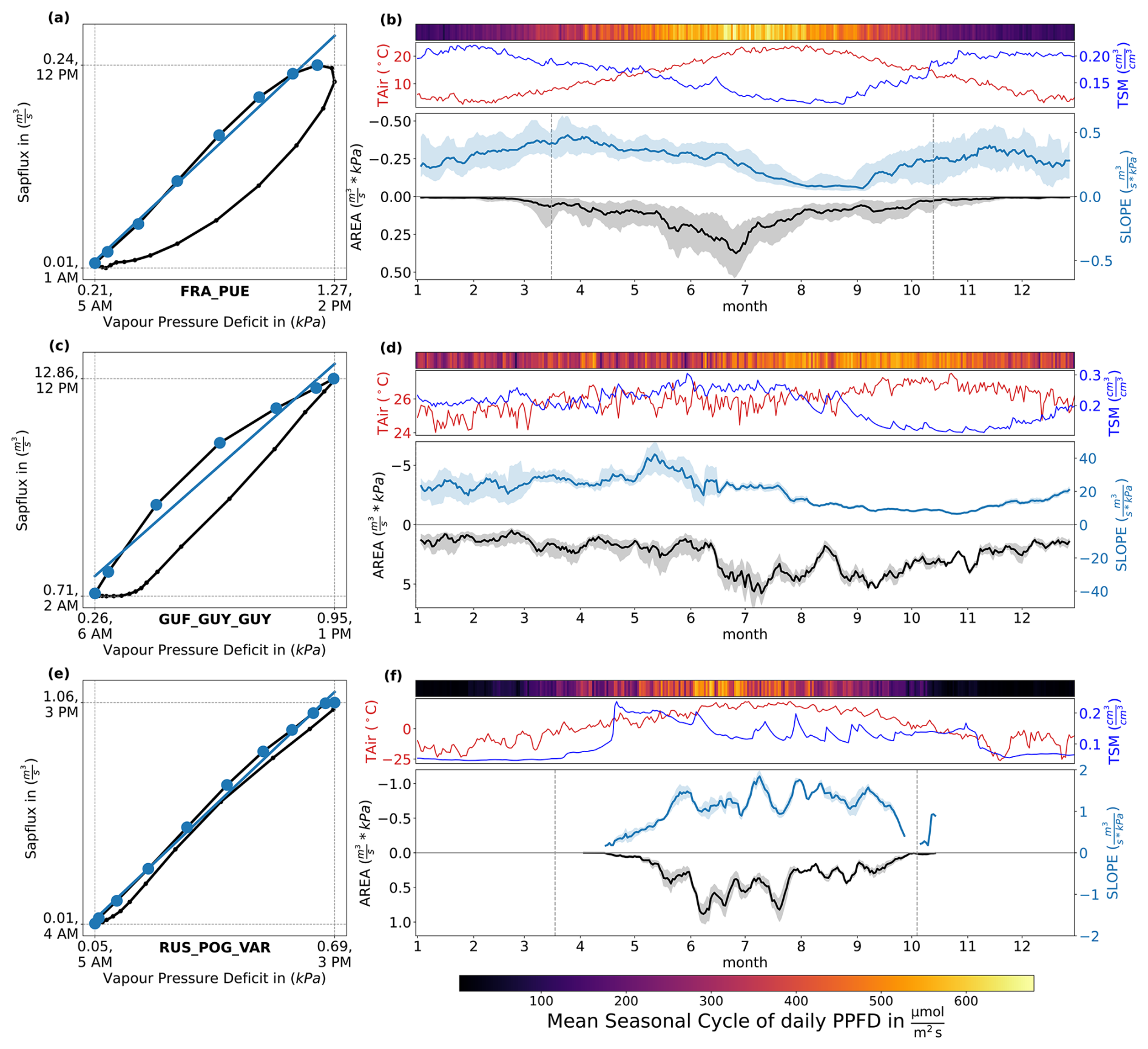
Figure 3 Illustration of metrics derived from diurnal SF-VPD relationships and their variability across seasons. (a, c, e): Illustration of the approach used to calculate the two metrics used in this study, based on the mean diurnal cycle of hourly VPD and SF measurements, aggregated over all trees and all days for the whole time span of available data for three selected sites: FRA_PUE, GUF_GUY_GUY, RUS_POG_VAR. The morning slope (SLOPE) is calculated through a linear regression of all hours (colored blue) between minimum VPD and maximum SF, while the area (AREA) is the area enclosed by connecting the data points for all available hourly timestamps. The dashed vertical and horizontal lines indicate the maximum values of the mean seasonal cycles of VPD and SF, and the corresponding average time of the day. (b, d, f): Seasonal dynamics of daily values of photosynthetically active radiation (PAR, quantified as daily PPFD), air temperature (T_Air) and top soil moisture (TSM), AREA and SLOPE with interquartile ranges showing the range of the hydrometeorological drivers and the derived metrics per day across years. The vertical lines indicate the selected growing season, i.e. when the day length is higher than 12 h and temperature > 5 °C. Absolute values of SLOPE vary according to the magnitude of tree-specific SF rates.

3 Results

3.1 Sub-daily and seasonal dynamcis of SF–VPD and hydrometeorological drivers

3.1.1 Seasonality of sub-daily hysteresis captured by daily metrics

The mean diurnal cycle of the bivariate relationship between SF and VPD for each of the focal sites (FRA_PUE, GUF_GUY_GUY, RUS_POG_VAR) is shown in Fig. 3a, c, e, together with the mean seasonal cycles of the two metrics derived from these diurnal hysteresis curves (AREA and SLOPE), shown in Fig. 3b, d, f. Note that the two metrics based on the diurnal SF-VPD cycles have daily time steps.

On average, hourly SF and VPD show very low (close to zero) values during night-time, with SF increasing as VPD increases through the morning. SF peaks around peak VPD for the three sites, before declining through the afternoon into the evening, in response to decreasing VPD. The absolute rates of SF, as well as the peak times of SF and VPD vary across sites. As a result, the degree of hysteresis in an average diurnal cycle and the slope of the curve in the morning (represented by the blue lines) also differs across sites, which we discuss individually below.

At FRA_PUE (panel a and b), the average diurnal cycle shows peak SF occurring around solar noon before peak VPD, which occurs around 02:00 pm on average. The morning SF aligns closely with rising VPD, with the rate of SF increase per unit of VPD increase in this period reflected by SLOPE. The rate of increase of SF with VPD begins to drop off in the late morning (after 10:00 am), and remains depressed relative to decreasing VPD throughout the afternoon, leading to a characteristic hysteresis loop, whose aperture is captured by the AREA. Similarly to FRA_PUE, the average diurnal cycle also shows a hysteresis at GUF_GUY_GUY (panel c and d), but here, hysteresis appears to emerge as a result of stomatal restrictions on SF initiating earlier in the morning (breakpoint at 09:00 am). Timings of peak SF and VPD align at 12:00 pm and the afternoon SF is aligned with VPD, with a strong stagnation at night close to minimum SF until SF starts to rise again in the morning. Despite these differences, the morning slope of the hysteresis curve similarly responds to changes in TSM, with slopes of 20–40 m³ s kPa⁻¹ during the wettest part of the year (January–July), decreasing to a minimum of approx. 8 m³ s kPa⁻¹ in November, when soils are driest. AREA is closely related to PPFD, but as observed at FRA_PUE, AREA starts to decrease in the driest parts of the year when SLOPE is suppressed by lower TSM values. In contrast, at RUS_POG_VAR (panel e and f), the average diurnal cycle of SF is aligned with the diurnal cycle of VPD with very little hysteresis (lower left panel), with maxima of both variables at 03:00 pm and minima at 05:00 am and 04:00 am, respectively.

The daily values of SLOPE and AREA derived from diurnal SF–VPD curves also show distinct seasonal variability patterns. In FRA_PUE, SLOPE values vary from approx. 0.2–0.5 m³ s kPa⁻¹ during January to April, decreasing slowly through late spring and more abruptly with the decline in TSM during the summer months, where SLOPE values close to 0 m³ s kPa⁻¹ indicate strongly limited hydraulic transport. SLOPE gradually recovers in autumn as TSM recharges. In contrast, AREA values follow more closely the seasonality of PPFD, peaking in June, before declining as water limitation suppresses the SLOPE of the morning limb of the hysteresis curve. The interannual variability in SLOPE and AREA, given by the spread around the mean values, is generally greatest outside the core of the dry season.

In GUF_GUY_GUY, SLOPE remains constant at about 20–40 m³ s kPa⁻¹ during the wet season (January–July), decreasing over the dry season to a minimum of approx. 8 m³ s kPa⁻¹ in November, when soils are driest. AREA shows less marked seasonality than the other two sites, but with a peak right before the start of the dry season around mid-July to August, and remaining high throughout the dry season (late July to November). At RUS_POG_VAR, AREA shows an increase at the onset of the growing season (May to June), but then showing variability throughout summer months, and followed by a fast decline from August onward. Contrary to FRA_PUE, SLOPE increases markedly at the start of the growing season and remains high, with strong sub-seasonal variations, until around September, when it decreases sharply.

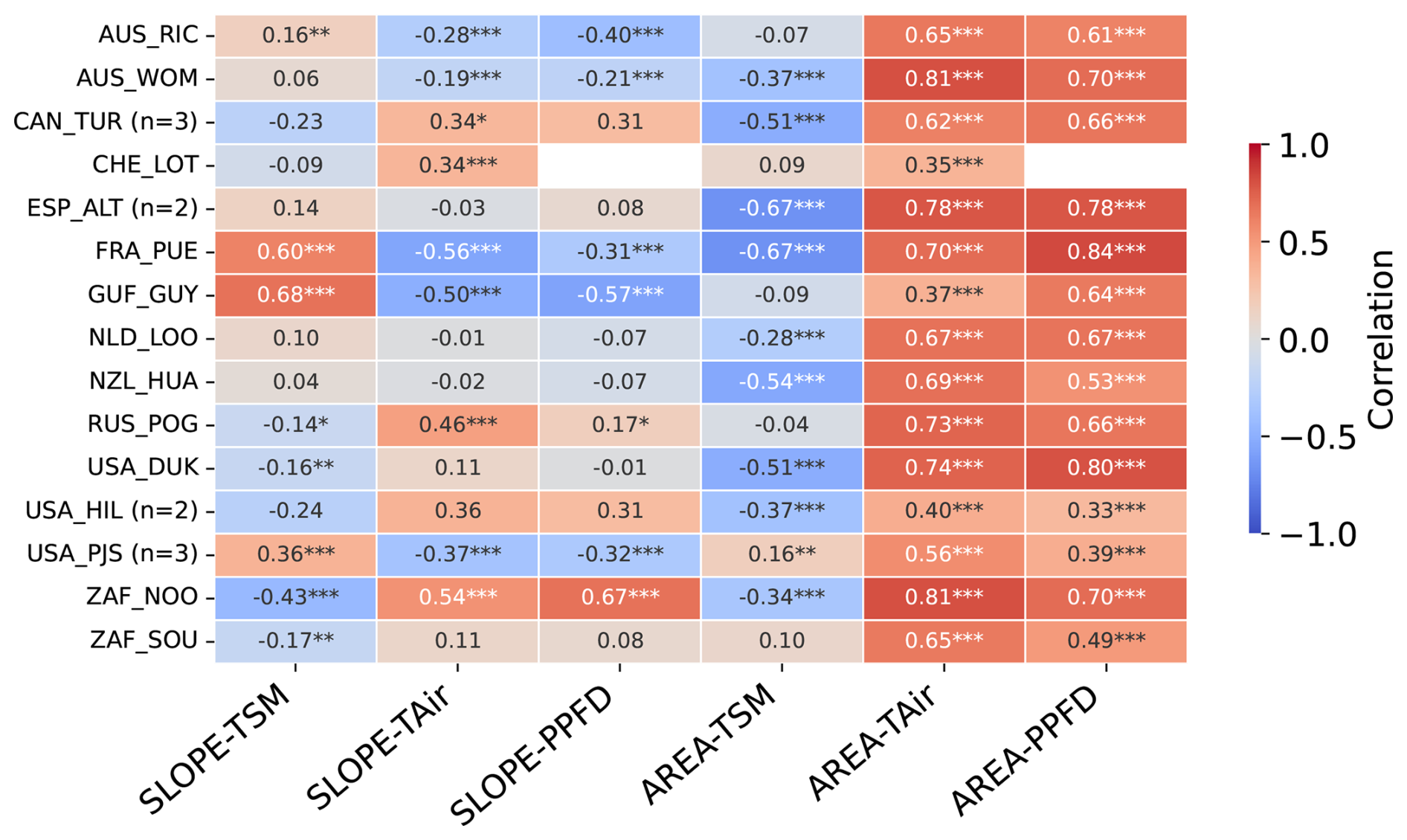
Figure 4 Heatmap of Pearson's correlation coefficients of the daily values of the SLOPE and AREA metrics and of hydrometeorological drivers (TSM, T_Air and PPFD) over the growing season across all studied sites. The number of plots at sites with multiple plots is indicated by n. Asterisks denote statistical significance, with three asterisks indicating p<0.001, two indicating p<0.01, and one indicating p<0.05.

3.1.2 Relation of SLOPE and AREA to climate drivers

Here, we analyse the relationship of SLOPE and AREA metrics and hydrometeorological drivers through the correlation of daily mean values of T_Air, PPFD, and TSM and the daily values of the AREA and SLOPE over the growing season for the broader selection of fifteen SAPFLUXNET sites, shown in Fig. 4.

Across all 15 sites, AREA correlates positively and with comparable magnitude with T_Air and PPFD (Fig. 4), while AREA and TSM tend to correlated negatively, with larger variations across sites. For the focal sites, GUF_GUY_GUY shows a much weaker relationship between AREA and temperature (R=0.37, Pearson correlation) than AREA and PPFD (R=0.64), while FRA_PUE shows the strongest correlation between AREA and PPFD across all sites.

The relationship of SLOPE with hydrometeorological drivers varies more across sites than for AREA, but with three groups that can be distinguished. A first group of five sites (AUS_RIC, AUS_WOM, FRA_PUE, GUF_GUY and USA_PJS), shows predominantly positive correlations between SLOPE and TSM (R=0.16 to 0.68), and negative correlations of SLOPE with T_Air ($R=-\mathrm{0.56}$ to −0.19) and PPFD ($R=-\mathrm{0.57}$ to −0.21), while another group of seven sites (CAN_TUR, CHE_LOT, USA_HIL, USA_DUK, ZAF_NOO, ZAF_SOU, RUS_POG_VAR) shows the opposite pattern: negative correlations of SLOPE with TSM ($R=-\mathrm{0.43}$ to −0.16, not significant for CAN_TUR) and positive or no relationship with T_Air and PPFD (R=0.46 to 0.54 and R=0.17 to 0.67, for significant values only). The remaining sites show no significant correlation between SLOPE and any of the three hydrometeorological variables. These differences appear to be associated with hydrometeorological regimes, with the first group predominantly associated with sites with marked dry seasons and the second group corresponding to cold/temperate sites, or sites in semi-arid regions but where irrigation is practiced (Table A2).

3.2 Diurnal SF–VPD dynamics during extreme conditions

Next, we compare diurnal SF-VPD dynamics and the associated AREA and SLOPE values under varying hydrometeorological conditions, classified according to combinations of upper and lower 20 % percentiles of T_Air and TSM (Fig. 5, and see Section 2.2). This procedure yields four clusters of moderate to extreme cold and wet, hot&wet, hot&dry and cold&dry conditions. The clusters and their corresponding mean diurnal cycles of absolute SF-VPD are illustrated for the three focal sites in Fig. 5. Given that we selected the three sites based on their different climate zones, the values of T_Air and TSM differ strongly in their absolute ranges for the different clusters as does absolute SF, given the differences in evaporative demand, but also differences in DBH and leaf area index (Table A1). Nevertheless, this clustering approach allows us to compare relative responses of SF-VPD dynamics to different to hydrometeorological conditions and evaluate how the SLOPE and AREA metrics reflect these responses.

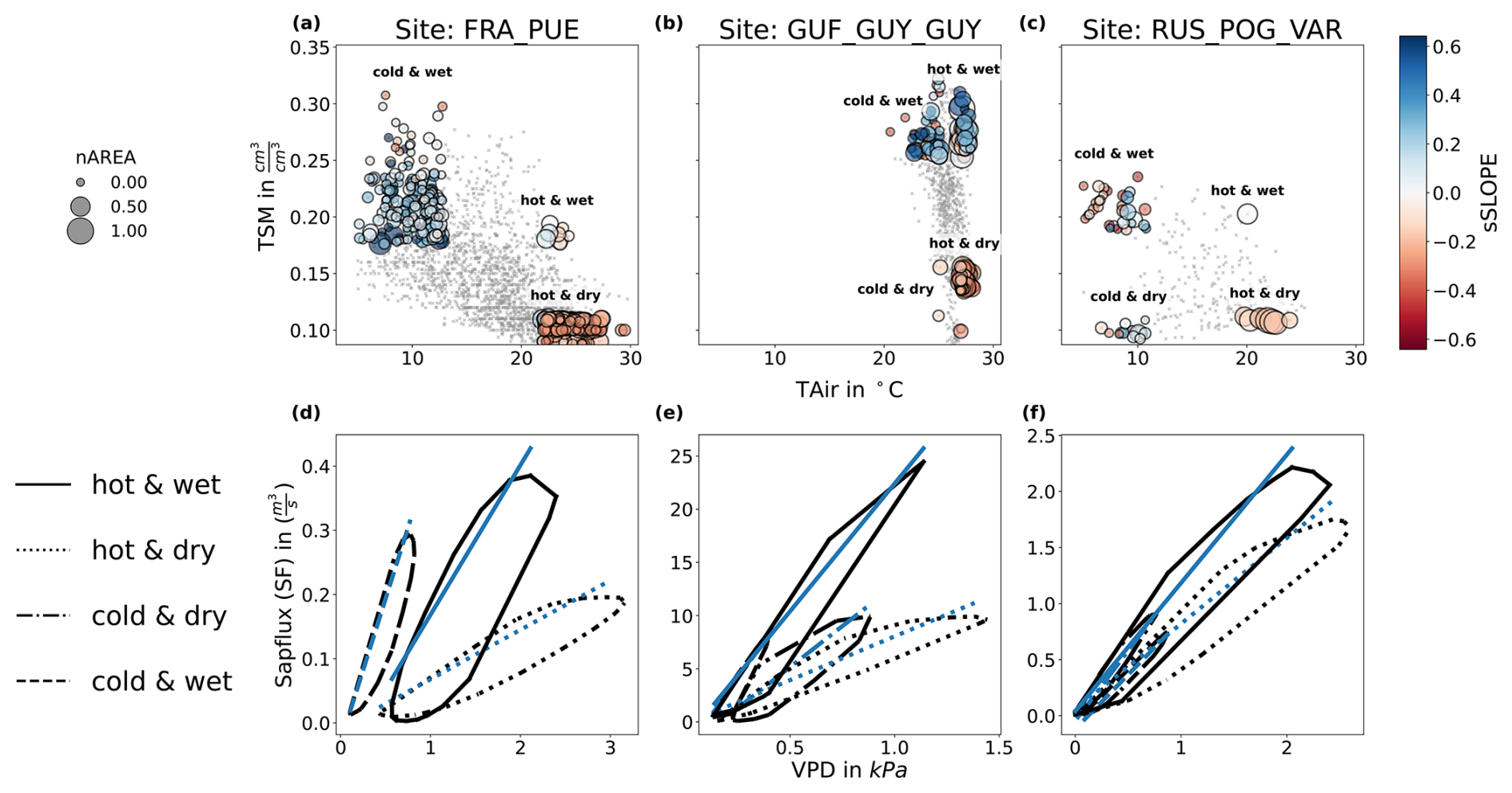
Figure 5 Changes in the SF–VPD diurnal cycles in response to varying hydrometeorological conditions. (a–c): daily mean values of absolute T_Air and TSM for each focal site (upper panel) and the four clusters corresponding to different combinations of the upper and lower 20 % percentiles of daily mean T_Air and TSM. The markers are colored by the corresponding values of sSLOPE and scaled by sAREA (d–f): Mean diurnal cycles of hourly VPD (x-axis) vs. SF (y-axis) for each of the focal sites, and for the four clusters corresponding to different hydrometeorological regimes: hot&wet (black solid line), hot&dry (black dotted line), cold&dry (black dash-dotted line), cold&wet (black dashed line). The corresponding SLOPE is shown in blue for each of the four curves, per site.

Across the three focal sites, and despite their different background climate, sub-daily dynamics exhibits similar responses to the different hydrometeorological clusters (Fig. 5). Hot days, generally reaching higher VPD values, are characterized by higher hysteresis (and thus higher AREA values) than cold days at all three sites. However, hot and wet days tend to be associated with steeper morning and afternoon slopes compared to hot and dry days, with the latter associated with a lower morning SLOPE, which is indicative of suppression of SF when soil moisture is most likely to be a limiting factor, even under very high VPD.

Despite these similarities, we also note differences between the three sites (Fig. 5). FRA_PUE shows the clearest separation between hydrometeorological regimes (panel a and d): cold–wet days are associated with low values of AREA with high SLOPE values, hot–wet days show high AREA values with reduced SLOPE and the highest peak SF, and hot–dry days reveal negative SLOPE anomalies with lower AREA than hot–wet days but still higher than cold–wet days. At this site, nighttime VPD minima do not return to zero in hot days, although SF can still cease. GUF_GUY_GUY (panel b and e) also shows contrasting dynamics for high- and low-TSM regimes, although it is worth noting that dry days are still considerably wetter than dry days in FRA_PUE and RUS_POG_VAR. SLOPE is higher for the wet regimes than dry ones, while AREA is higher in hot days than cold days, although the difference of hot versus cold is only 5 °C at this site. At hot-wet days, peak SF exceeds all other regimes by more than a factor of two. In RUS_POG_VAR (panel c and f), hot conditions are associated with higher AREA and dry days are associated with lower SLOPE, although the variability observed in SF–VPD hysteresis between relative hydrometeorological extremes at this site is less marked than at FRA_PUE and GUF_GUY_GUY.

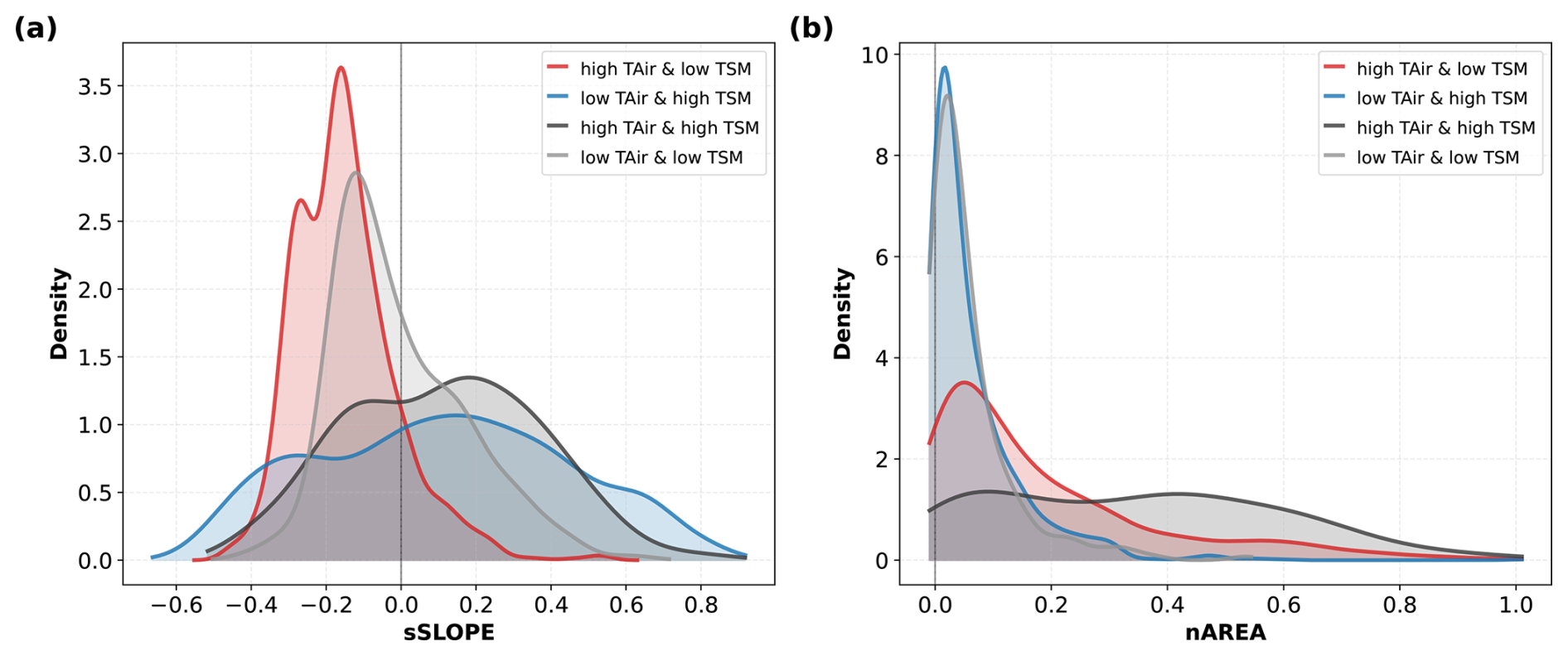
Figure 6 Distribution of (a) sSLOPE and (b) nAREA at extreme anomalies of T_Air and TSM for all 15 sites for different groups of hydrometeorological extremes, as shown in Fig. 5 for the three representative sites. Red curves correspond to hot and dry days (high T_Air and low TSM), blue curves to cool and wet days (low T_Air and high TSM), black curves to hot and wet days (high T_Air and high TSM) and grey curves to cool and dry days (low T_Air and low TSM).

Based on these results, the AREA and SLOPE descriptions appear to reflect characteristic hydrometeorological regimes across the three focal sites, allowing to distinguish distinct types of responses to environmental stressors. To evaluate whether these differences can be generalized across sites, we analyse the distributions of sSLOPE and nAREA at all 15 sites during the four types of hydrometeorological regimes (Fig. 6).

For the standardized SLOPE (sSLOPE, panel a), distributions show significant differences between wet and dry hydrometeorological regimes: for both cold and hot days with high TSM, the distributions of sSLOPE show a large spread with positive median values (median =0.12), while for days with low TSM, the distributions are strongly skewed towards negative sSLOPE values, with median values of −0.16 and −0.05 for hot and dry and cold and dry days, respectively.

In the case of the normalized values of AREA (nAREA, panel b), we find stronger differences in the between hot and cold hydrometeorological regimes: cold days show a predominance of very small values, and very similar distributions for cold days whether the soil is wet or dry, with comparable median values (0.03) and a similar tail distribution. By contrast, hot days show very long tails and median values shifted towards higher values (0.11 and 0.35 respectively), which is particularly pronounced for the regime corresponding to hot conditions and high TSM.

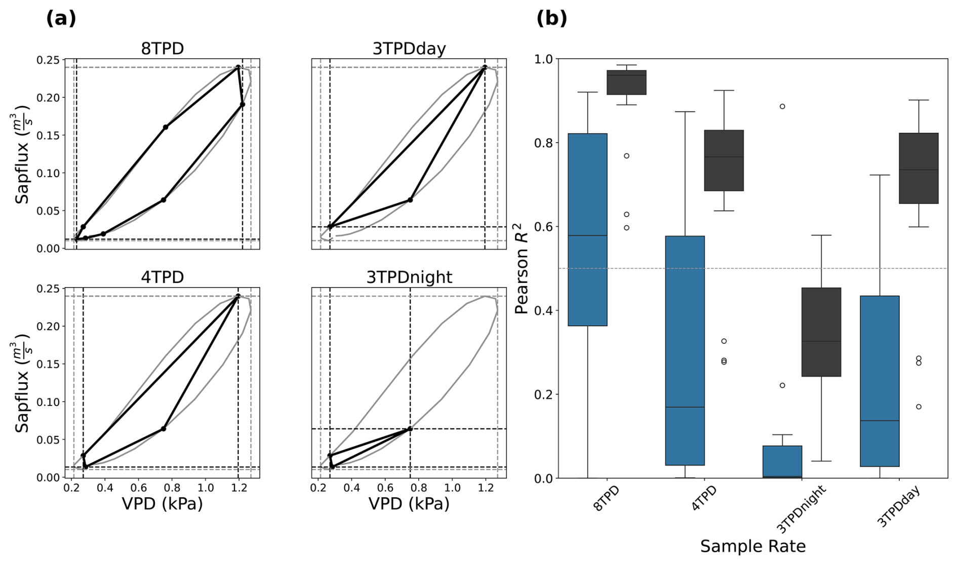
Figure 7 Effect of temporal resolution and sampling times on the two diurnal cycle metrics. (a): illustration of the average diurnal cycle for FRA_PUE, estimated based on hourly measurement (solid gray lines), and the corresponding diurnal cycle captured by measurements at different sample rates (bold black lines). The vertices of the curves under lower sampling rates indicate the observations at different sampling rates: 3-hourly, starting at mid-night (8 times per day, 8TPD), 6-hourly, starting at mid-night (4TPD) and 6-hourly with mid-night or noon left out (3TPDday, 3TPDnight). The vertical and horizontal dashed lines indicate the corresponding maximum values of the reference diurnal cycle with hourly time steps (gray) and with coarser temporal sampling (black). (b): Boxplots of coefficients of determination (R²) estimated as the relationship between daily time series of the AREA (black) and SLOPE (blue) metrics at different sample rates (x-axis) and the reference values derived from hourly sampling. The boxplots summarize the variability of R² across all sites and reflect how closely the seasonal dynamics of the metrics based on resampled time series track those of the hourly reference across sites.

3.3 Dependence of sub-daily metrics on sampling rate

While in situ sensors can provide continuous sap flow data, we consider the potential to estimate these descriptors of the diurnal cycle using temporally sparse data (see Sects. 1 and 2.2). In particular, as sap flow is connected to changes in water storage, which can be estimated using microwave remote sensing, we examine the degree to which the SLOPE and AREA can be estimated for several acquisition strategies with different numbers of observations and acquisition times.

Figure 7b) shows the distribution of the coefficients of determination (Pearson R²) obtained by linear correlation of the daily values of the SLOPE and AREA metrics derived from the hourly data, and those derived from sparser sub-daily sampling frequencies and the values for each site. We tested frequencies ranging from 8 (3-hourly), 4 (6-hourly), and 3 (6-hourly with either mid-night or mid-day left out) times per day (TPD) starting at 6am, as illustrated in Fig. 7a for FRA_PUE.

The AREA descriptor calculated with coarser temporal sampling agrees well with the AREA estimated using hourly data, though the agreement obviously declines when fewer data are used in the estimation. With 8TPD, the AREA values are well preserved, with a median annual Pearson R² of 0.95 and an interquartile range of 0.9–0.97. For 4TPD, the relationships between AREA values derived from sparse sampling and the higher temporal resolution become weaker and less well constrained, as given by the median correlation of 0.76 and interquartile range of 0.67–0.83. There is very little further information loss in AREA estimation when sampling at 3TPD when there is an observation at noon (3TPDday, median R²: 0.74; IQR: 0.66–0.83). However, there is significant degradation in the relationship for 3TPDnight, where the observation at noon is missing (median R²: 0.30; IQR: 0.22–0.45)

Compared to AREA, the estimates of SLOPE are more sensitive to sampling frequency and exhibit greater variability across the sites, especially at 8TPD. At 8TPD, the correlation with the hourly sampling shows a median value of 0.5 with interquartile range of 0.26–0.82. Similarly to the performance of AREA, the agreement of SLOPE calculated with lower sampling rates deteriorates with decreasing frequency: with median correlations of 0.16, 0.01 and 0.14 for 4TPD, 3TPDnight and 3TPDday, respectively. Furthermore, the correlations of SLOPE for 4TPD and 3TPDday show large spread, with interquartile ranges of 0.03–0.55 and 0.02–0.37, respectively. In general, AREA is underestimated at lower sampling frequencies.

The diurnal cycles of SF–VPD under sparse sampling, shown in Fig. 7a), illustrate the poor performance of 3TPDnight in estimating SLOPE at least for FRA_PUE. 3TPDnight cannot accurately capture maximum SF (see Fig. 7a), even though it does effectively capture minimum VPD. In contrast, 4TPD and 3TPDday slightly overestimate minimum VPD but still yield better SLOPE estimates, with 3TPDday performing best among the reduced sample rates.

With the sample times considered, maximum VPD tends to be underestimated, reducing accuracy in metrics relying on its diurnal extremes at this site. Nevertheless the sample rates of 4TPD and 3TPDday still capture the metrics similarly at all sites, with better results of AREA at 4TPD and better results for SLOPE at 3TPDday.

4 Discussion

4.1 Metrics as indicators for tree stress

Sap flow (SF) alone is not a reliable indicator of vegetation response to environmental conditions, because absolute rates depend on tree size, species, and stand conditions (Wheeler et al., 2023; Chen et al., 2012). This is seen by the large differences in absolute SF across the three selected sites (Fig. 5). Instead, previous studies have shown that diurnal SF–VPD dynamics provide clearer insight into regulation processes (Poyatos et al., 2016; Renninger et al., 2021). Therefore, the diurnal cycle of SF-VPD provides diagnostic indicators that consistently discriminate the drivers of extreme stress across all fifteen forested sites. Here we propose that two such indicators can be used in combination to identify characteristic responses to changing environmental conditions, and particularly hydrometeorological extremes. Our results show that the morning SLOPE and the AREA of the diurnal cycle of SF-VPD vary across seasons and systematically change from cold–wet to hot–dry conditions across most sites. Our results indicate that the combination of higher climatic demand and lower soil water availability reduce the coupling of SF to VPD.

We have shown, that cold and wet conditions correspond to high SLOPE and low AREA of the diurnal cycle (dashed lines in Fig. 5, blue curves in Fig. 6), as SF aligns tightly with VPD and hysteresis is minimal. This dynamics indicates a strong coupling of SF and VPD, i.e., under conditions of limited demand and high supply, trees exhibit weak stomatal regulation, prioritizing carbon uptake over preventing water losses. By contrast, in hot and dry conditions (dotted lines in Fig. 5, red curves in Fig. 6), AREA increases and the SLOPE declines, reflecting the onset of regulation of SF before peak VPD and stagnation of SF during periods of high atmospheric demand. These patterns may result from increased stomatal regulation or limitations to plant hydraulic water supply.

Despite these general patterns, the variations of SLOPE and AREA and their relationships to hydrometeorological drivers differ among climate zones (Fig. 4). AREA shows consistently positive correlations with T_Air and PPFD across sites, indicating a robust response to atmospheric energy availability that is largely independent of climate regime or plant group. In contrast, correlations between AREA and soil moisture are weaker and more variable, suggesting that AREA integrates canopy responses that are only indirectly constrained by short-term water availability.

The relationships between SLOPE and hydrometeorological drivers are markedly more site-dependent. Sites with pronounced dry seasons show positive correlations between SLOPE and soil moisture and negative correlations with T_Air and PPFD, consistent with water-limited canopy dynamics. Conversely, cold and temperate sites, as well as semi-arid sites with irrigation, exhibit negative or no correlations between SLOPE and soil moisture and positive or neutral relationships with energy-related drivers, suggesting that irrigation at otherwise water-limited sites may dampen or mask typical stress-related responses. Overall, AREA behaves as a broadly comparable metric across ecosystems, primarily reflecting energy limitation, whereas SLOPE is strongly shaped by local hydrometeorological regimes and management. Together, both metrics capture differences in the strength of biosphere–atmosphere coupling.

The full exploration of the complexity of the correlations between metrics and climate drivers is beyond the scope of this analysis. Furthermore, different responses of the metrics were found across sites, but still they help to reveal whether down-regulation occurs under increasing atmospheric demand. The underlying cause of down-regulation, be it stress, adaptive behavior, or species-specific traits—must be interpreted in context. Next to site-specific differences, the still short SAPFLUXNET time series limit the calibration of the metrics against long-term means. Without such references, it remains uncertain whether regulation corresponds to stress or adaptive behavior. Importantly, a lack of regulation does not necessarily indicate optimal conditions; it may instead signal failure to respond to stress or overshooting, risking excessive water loss and hydraulic damage (Schymanski et al., 2013; Lawson et al., 2011; Jones et al., 2022; Sperry and Love, 2015).

The metrics derived from the SF–VPD relationship thus can serve as early indicators of regulation patterns and water use strategies, some of which can be attributed to stress (Gambetta et al., 2020; Bodner et al., 2015; Brunner et al., 2015; Seleiman et al., 2021; Acosta-Motos et al., 2017). While SLOPE measures the strength of the coupling between SF and atmospheric demand, the AREA is an indicator of regulation timing in relationship to the atmospheric demand. Combining SLOPE and AREA helps to reduce ambiguity, as in the diagnostic case of low SLOPE with high AREA, which can be used as an indicator for strong regulation. Still, limitations remain: coarse temporal resolution may miss the identification of downregulation from breakpoint patterns in morning SF, and lack of regulation over consecutive days may reflect either risky strategies or optimal conditions. While interpreting these metrics requires integration with local water balance, species traits, and climatic drivers, they can serve as a useful proxy to detect changes in vegetation functioning in response to environmental conditions.

4.2 Evaluation of the state of ecosystems in focus

More detailed assessment of the hydraulic hysteresis reveals novel insights into the variation in physiological dynamics across sites, with implications for understanding their adaptation to existing climate and potential vulnerability to future climate extremes.

At the Mediterranean site (FRA_PUE), stomatal regulation is triggered when atmospheric and soil moisture drought coincide (Fig. 3), reflecting interactions between water and temperature, through VPD. The sensitivity of AREA and SLOPE to both atmospheric demand and TSM is shown by the sign and strength of the correlation with all hydrometeorological drivers (Fig. 4). Furthermore, the negative correlation of AREA with TSM indicates that stomatal closure is a primary response when topsoil water becomes a limiting factor. Increasing AREA signals moderate regulation at high temperature, while declining SLOPE throughout the day represents strong conservative water use under severe diurnal drought and heat stress, triggering stomatal closure (Figs. 4, 5, 6). A strong ability to close stomata is also indicated, when SF is absent at night at non-zero VPD. This site also has the widest range in T_Air and TSM, which are as well negatively correlated, suggesting that plants frequently operate near or at their physiological limits. While the adaptation strategies have traditionally allowed these species to withstand seasonal drought, the additional compounding stress from increasing heat and VPD leaves them vulnerable to conditions that exceed historical variability (Ruffault et al., 2023; Limousin et al., 2022). Thus, the site’s long-term water conservation strategies, although beneficial in historical contexts, now signal a heightened exposure to future extreme events. Empirical evidence of recent mortality supports the conclusion that these adaptive strategies are being overcome under more severe and compound climatic stresses (Peguero-Pina et al., 2020; Allen et al., 2015; Aurelle et al., 2022).

In contrast, stomatal regulation at the tropical site is less sensitive to heat. Here, the SF–VPD dynamics is mostly controlled by radiation and soil moisture (Fig. 4), where seasonal drought results in the decreasing of the morning SLOPE. AREA primarily reflects afternoon or nighttime stagnation of SF, which can also be a sign for high TSM enabling the trees to maintain SF during the night (Fig. 5). Previous studies have shown the strong importance of VPD for SF dynamics in these regions (Horna et al., 2011; Maréchaux et al., 2018; Suárez et al., 2021), here we show that radiation still contributes to modulate the sensitivity of SF to VPD, as seen by the strong correlations between AREA and SLOPE with PPFD and TSM (Fig. 4). At this site, tree height and hydraulic structure likely contribute to the high absolute SF rates, supported by deep rooting and access to water beyond topsoil layers (Horna et al., 2011; Apgaua et al., 2015; Kotowska et al., 2021; Spanner et al., 2022). The results highlight an ecosystem optimized for heat under conditions of high water supply. Trees at this site are capable of transpiring large volumes of water to maintain levels of high stomatal conductance and photosynthesis.

The Russian site displays an inverted response pattern compared to the warm sites: SLOPE and AREA increase and decrease together at the beginning of the season until they are aligned (Fig. 3), which is supported by the strong correlation of AREA-PPFD and AREA-T_Air (Fig. 4). The cluster analysis (Fig. 5) indicates that the trees at this site are predominantly energy-limited, with an optimal temperature threshold, which is likely to be occur earlier within a season with rising temperatures (Berner et al., 2013). Contrary to the other two sites, SLOPE decreases with increasing TSM, thus contradicting the expectation that additional water would sustain SF. The variability of AREA throughout summer months might be linked to cloud cover. This suggests unusual or site-specific regulation dynamics, potentially influenced by snow melting early in the season, growth and senescence of the larch canopy, or the fact that the seasonal drought is often outside of the growing season (see Fig. 3). The overall absence of strong stomatal downregulation at this site suggests that trees follow a non-conservative water-use strategy, possibly at the risk of depleting water for more carbon uptake. However, this may mask delayed stress onset or increased vulnerability to prolonged warming (Liu et al., 2022; Urban et al., 2017; Ruehr et al., 2019, 2015).

Projected climate change will likely intensify the stressors already identified here. In Mediterranean regions, increased frequency and duration of hot–dry extremes may amplify regulation and risk hydraulic failure, pointing to high vulnerability. In tropical forests, warming and drying may shift regulation triggers, potentially exposing hidden hydraulic limitations despite deep water access. At cold continental sites, continued warming may lift energy constraints, increasing SF without corresponding regulation–yet such non-conservative strategies may conceal longer-term risks of water imbalance.

4.3 Metrics and Sample Rates

Current research is actively exploring how satellite-based measurements of VWC, e.g., through vegetation optical depth (VOD) or other microwave observables, and derived indicators of plant water status can contribute to a more in-depth understanding of plant health and ecosystem dynamics (Schneebeli et al., 2011; Momen et al., 2017; Holtzman et al., 2021; Humphrey and Frankenberg, 2023; Asgarimehr et al., 2024). The need for diurnal measurements of VWC to better quantify vegetation responses to drought has been highlighted by Konings et al. (2021). As discussed in Sect. 1 and Fig. 1, sub-daily satellite observations of vegetation water storage from microwave remote sensing can in principle be used to derive sub-daily variability in SF dynamics, a variable more directly related with plant functioning.

Here, we analysed the effect of temporal resolution on the two metrics proposed. This allows us to evaluate, in cases where 30 min or hourly resolution is not feasible, e.g., for remote-sensing applications, what the minimum temporal resolution would be required in order to adequately capture the SF–VPD dynamics. Generally, no sample rate can capture all details of the diurnal cycle as constrained by the hourly data (Fig. 7).

The 8TPD represents an ideal case assuming unlimited observations or coverage, consistent with characteristic frequencies from geostationary satellites for example. While time series from measurements at 8TPD exhibit very good correlation with the reference from hourly observations of SF and VPD for AREA, the results for SLOPE already show a degradation of the signal, with a broad spread across sites. For lower sample rates, results for both metrics are less accurate than for 8TPD, with the 75 % percentile for SLOPE already falling below 0.6 at 4TPD. Compared to 4TPD, the correlations of 3TPDday for SLOPE demonstrate only slight differences, since only nighttime is excluded, where sap usually does not flow significantly. Therefore, measurements at 3TPDnight, which include only nighttime flux, would not be a suitable choice for both metrics.

The mixed correlation results of SLOPE from resampled SF and VPD are likely due to the low signal-to-noise ratio of the hourly metric itself. These mixed results originate in dynamics resulting in negative SLOPE or high positive and negative outliers, such as rainy days or dew, which are hard to interpret. It is possible that SLOPE calculated from SF and VPD at lower sample rates could better infer the signal needed for early warning of tree stress hotspots by neglecting the values of SF and VPD that produce outliers. Another potential reason for the low accuracy of SLOPE from resampled observations is the possibility of both under- and overestimation, depending on the hysteretic behavior of the diurnal cycle, which shifts the maximum value of VPD behind the maximum of SF. Furthermore, the peak times of SF and VPD at some sites (e.g. the russian site) did not match solar noon. While the dynamics at the proposed times and sample rates would be well captured at FRA_PUE and GUF_GUY_GUY, both metrics of the diurnal cycle could be underestimated at sites with dynamics similar to RUS_POG_VAR.

These results raise the question of whether the choice of metrics is adequate to capture the diurnal cycle of SF and VPD from satellites and how they can be improved. AREA is generally underestimated, but relative trends in AREA tend to be consistently retrieved with coarser temporal resolution. SLOPE has lower Pearson R² than AREA, however, the relative trends are still sufficient to indicate water limitation at most sites. Nevertheless, alternative approaches should be evaluated. For example, instead of the absolute slope, the ratio of the actual to a potential morning regression slope could be considered. This metric could identify collapse days, when the ratio is high, and exclude outliers when it exceeds 1. The challenge here mainly lies in how a potential slope could be defined.

The reduced variance of the metrics under high environmental stress conditions indicates a stabilization of underlying processes and enhances the predictability of stress patterns during these periods. Therefore, SLOPE and AREA can detect early warning signs of SF regulation, which indicates tree health, from the sub-daily response of SF to VPD, which could then be further investigated in detail through in situ observations to enhance our knowledge of specific stress responses outside of laboratory settings and mitigate subsequent tree mortality events. For this purpose, a sample rate of 3TPD centered at day-time, would suffice.

4.4 Linking fluxes to storage

One limitation of the current study is the reliance on sap flow data (a flux), while the the quantity more likely to be provided by satellite remote sensing is VOD (or derived VWC), a measure of vegetation water storage. Recall from Fig. 1 that the expected shapes of the hysteresis curves are different for SF and VWC. It is therefore possible that a SLOPE metric may be more reliably estimated when monitoring VWC rather than SF under a 3TPDday scenario. The application of conservation of mass to translate between the two is complicated by a mismatch in terms of the volume being considered. Sap flow measurements quantify the movement of water through the sapwood of individual tress. Although sensing depth of VOD and its sensitivity to water content in different compartments of the vegetation are known to depend on frequency, VOD (and derived VWC or biomass) are commonly assumed to represent storage of the vegetation as a whole, and spatially integrated across some footprint. Therefore, the dynamics observed in sap flow data, and the derived daily slope and area metrics should not be considered a trivial proxy for VOD or a change in VOD. That said, sap flow data reveal when transpiration is occurring which allows us to identify when, and the degree to which storage is likely to be changing at sub-daily scales. While it seems logical that steeper slopes and larger areas in sap flow would also result in similar changes in VOD, this should be confirmed with sub-daily VOD estimates from tower-based radars and/or radiometers and emerging GNSS-related techniques (Jagdhuber et al., 2025).

5 Conclusions

The aim of this study was to understand how sub-daily sap flow dynamics can be used as an indicator of vegetation functioning and stress and to evaluate the potential to estimate descriptors of the diurnal cycle using temporally sparse data. While sap flow alone has limited interpretability in assessing vegetation condition, its response to sub-daily atmospheric water demand variations can help identify different types of stress. We propose two simple descriptors of the diurnal cycle of SF–VPD, namely the morning sensitivity of SF to VPD (the slope) and the area of the hysteresis curve, that show clear seasonal and interannual variability patterns, associated with varying hydrometeorological conditions. As interpretion of either metric alone can be ambiguous, it is recommended that these metrics should be interpreted in combination.

Our results show that the descriptors of short-term dynamics in SF response to atmospheric water demand reflect responses to hydroclimatic stressors, and are particularly sensitive to extreme events, emphasizing the potential for observations of sub-daily vegetation water dynamics to monitor ecosystem vitality at larger scales. Given the lack of global measurements of SF or vegetation water content at high temporal resolution from which to derive such metrics, we show that a sampling rate of 3–4 times per day would be sufficient to derive the two descriptors proposed while retaining the information of the finer temporal resolution measurements. Our results thus show potential for temporally and spatially continuous measurements, e.g., from future satellite missions, to use sub-daily information about vegetation water content and fluxes to track plant stress as an early-warning indicator for mortality events. Therefore, enhanced vegetation monitoring through sub-daily satellite observations of vegetation water content could greatly improve ecosystem management strategies and climate change mitigation plans.

Appendix A

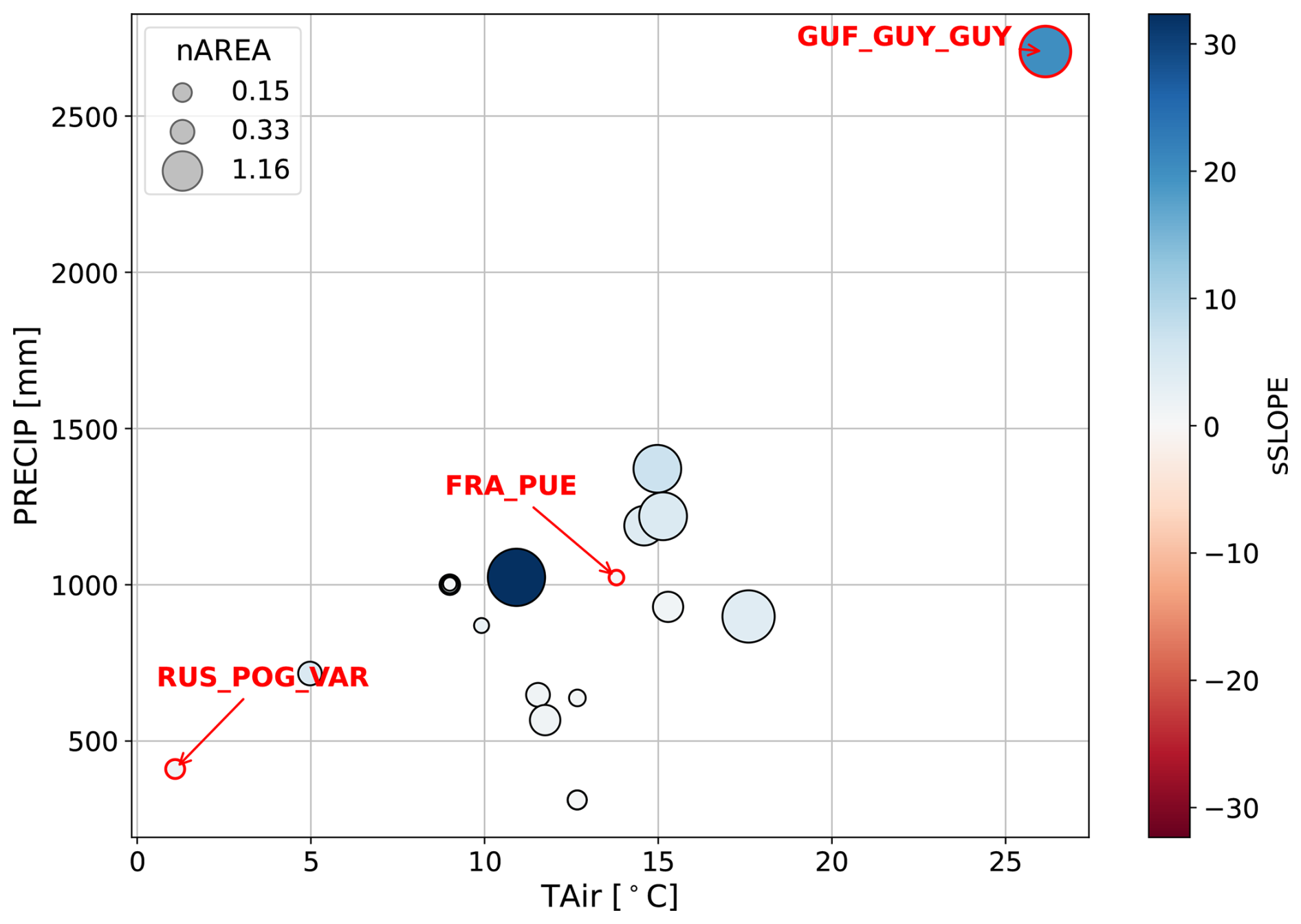
Figure A1 Mean precipitation and mean air temperature at each of the study sites. Symbol size scales with median sAREA and color indicates median sSLOPE per site across years with the three selected sites annotated and highlighted in red.

Table A1 Site characteristics including physical and biological attributes.

Table A2 Site treatments and references.