Divergent sensitivities of apparent oxygen utilization to ventilation changes in the deep ocean across Earth system models

The biological carbon pump (BCP), involving photosynthesis at the surface and remineralisation at depth, maintains a significant vertical gradient in dissolved inorganic carbon (DIC), thereby promoting the ocean's ability to absorb atmospheric CO₂. Remineralised DIC is a good indicator of the strength of the BCP. It can be estimated from apparent oxygen utilisation (AOU), which measures the deficit of oxygen relative to saturation. AOU is projected to increase under climate change due to changes in remineralisation rates and ventilation. However, the amplitude of the change remains uncertain. Here, we identify linear relationships between trends in AOU and ideal-age in the deep ocean, based on simulations of the contemporary (1982–2013) and future (2015–2099) periods from five Earth system models (ESMs). Our analysis underscores the substantial role of ventilation slowdown in increasing remineralised DIC. Furthermore, the study highlights considerable inter-model variability in their sensitivity of AOU to age changes, with this sensitivity remaining relatively stable over time. With more observational data, refined estimates of age changes from ocean tracers and a larger model ensemble, constraining this variability will become feasible. These insights emphasise both the challenges and opportunities for constraining future BCP projections arising from uncertainties in ventilation.

1 Introduction

The capacity of the ocean to take up and store carbon is driven by the marine carbonate chemistry, the solubility pump and the biological carbon pump (BCP hereafter, accounting for the carbonate and soft-tissue pumps, Volk and Hoffert (1985) and see DeVries (2022) for a review of the ocean carbon cycle). A part of the BCP is the photosynthetic transformation of inorganic carbon to organic carbon at the surface. The organic material is then transported to depth where it is transformed back into its inorganic form through remineralisation. In the deep ocean, remineralised carbon and nutrients are accumulated. This accumulation is an important component of the BCP and is connected to the strength of the ocean overturning circulation, which transports the inorganic carbon and nutrients back to the surface, closing the loop. The BCP is therefore the primary mechanism responsible for keeping the concentration of dissolved inorganic carbon (DIC) low at the surface and high in the interior, resulting in a large vertical gradient of DIC (Volk and Hoffert, 1985; Boyd et al., 2019; DeVries, 2022). This enhances the capacity of the ocean to take up atmospheric CO₂ (Kwon et al., 2009). Without the BCP, atmospheric CO₂ would be more than 200 ppm higher than otherwise (Sarmiento and Toggweiler, 1984; Maier-Reimer et al., 1996; Goodwin et al., 2008; Tjiputra et al., 2025).

Due to competition between the decrease in organic matter export and slower circulation, it is unclear how the role of BCP will change in the future (Frenger et al., 2024). There is a general consensus between state-of-the-art Earth system models (ESMs) that the BCP and the processes involved are impacted by global warming (Wilson et al., 2022), but the amplitude of the change and its response to higher atmospheric CO₂ are both still uncertain. Indicators of the functionality of the BCP are primary production (related to the photosynthetic transformation of carbon at the surface), export production (related to the transport of organic material to depth) and the amount of remineralised carbon. On average, ESMs project a decrease in globally averaged primary production and export production across various future scenarios of increasing atmospheric CO₂ (Henson et al., 2022; Wilson et al., 2022; Kwiatkowski et al., 2020). Yet, these results differ regionally with, e.g., a general increase in the Arctic Ocean, Southern Ocean, and a general decrease in the equatorial Pacific (Myksvoll et al., 2023; Henson et al., 2022; Wilson et al., 2022; Kwiatkowski et al., 2020). Globally and regionally, the range of projected changes in primary production and export production differs largely between ESMs such that the inter-model range of the change is often more than twice its multi-model mean (Tagliabue et al., 2021). In contrast, greater accumulation of remineralised carbon in the ocean interior can be expected due to a more sluggish circulation (Tjiputra et al., 2018; Weijer et al., 2020), increasing the effectiveness of the BCP despite a reduced export production from the surface (Liu et al., 2023). However, despite model consensus on a global increase of remineralised carbon across scenarios, the amplitude varies widely between models (Wilson et al., 2022).

The quantity of remineralised carbon (DIC_remin) is a good indicator of the strength of the BCP and its impact on atmospheric CO₂ (Marinov et al., 2008; Kwon et al., 2009; Koeve et al., 2020; Frenger et al., 2024). In a steady state climate, large DIC_remin stocks correspond to low atmospheric CO₂ levels (Marinov et al., 2008; Frenger et al., 2024) and in a transient climate, the strongest increase in DIC_remin corresponds to the strongest biologically-induced decline in atmospheric CO₂ (Koeve et al., 2020; Frenger et al., 2024). In contrast, export production is unrelated to atmospheric CO₂ (Marinov et al., 2008; Kwon et al., 2009; Frenger et al., 2024). DIC_remin can be estimated from apparent oxygen utilisation (AOU, Frenger et al., 2024; Wilson et al., 2022), which measures the deficit of oxygen compared to saturation. It is an estimate of the cumulative oxygen utilised to remineralise organic material since the water parcel was last in contact with the atmosphere. Despite some limitations such as assuming 100 % oxygen saturation at the surface (Ito et al., 2004), changes in AOU can be used for quantifying the impact of the BCP on atmospheric CO₂ (Koeve et al., 2020).

AOU is traditionally supposed to be the product of the oxygen utilisation rate (OUR) and an estimation of ventilation age, i.e. the time since the water-mass was last in contact with atmosphere (see for example Sulpis et al., 2023; Guo et al., 2023; Sonnerup et al., 2015; Feely et al., 2004; Sarmiento et al., 1990; Jenkins, 1982). In regions dominated by advection or with an even spatial distribution of the respiration rate, the relation between AOU and ventilation age is linear when both are affected similarly by transport (Koeve and Kähler, 2016). Typically the linear relationship breaks in areas where gradients are too different (Thomas et al., 2020). A stronger remineralisation closer to the surface or below highly productive zones (e.g., equatorial Pacific) will locally increase AOU without any correlation to a change in ventilation age. The linear relation between AOU and ventilation age has been used to estimate OUR (Sulpis et al., 2023; Jenkins, 1982) and as a proxy of water-mass age (Thomas et al., 2020). The relationship between trends or changes in AOU and ventilation age can further be used to decompose changes in AOU into ventilation-driven and biologically-driven factors. So far this relationship has been little explored in future climate projection. Bopp et al. (2017) found a strong relationship in one ESM from the Coupled Model Intercomparison Project Phase 5 (CMIP5), however, ventilation ages were not available for the other CMIP5 models. More recently, Liu et al. (2023) explored the relation between changes in circulation and changes in AOU. They found that the slowing down of the meridional overturning circulation, which is an indicator of ocean interior residence time, would allow more time for the exported biogenic carbon to accumulate at depth and thus increase the deep ocean storage of carbon by the BCP.

In this work we further explore the relationship between changes in circulation and changes in the BCP using Earth system model simulations from the sixth Coupled Model Intercomparison Project (CMIP6) as well as observations from the Global Ocean Data Analysis Project (GLODAPv2, Lauvset et al., 2024). Following the approach suggested by Frenger et al. (2024), we use remineralised DIC, estimated from AOU, as indicator for the BCP. We show that changes in AOU are linearly related to changes in ventilation age in large parts of the deep ocean. We further use the linear relationship to quantify the respective role ventilation changes play in the future evolution of the BCP. Lastly, we discuss future opportunities to constrain the estimates of the deep ocean BCP with observations.

2 Methods

2.1 Earth system models outputs and observational data

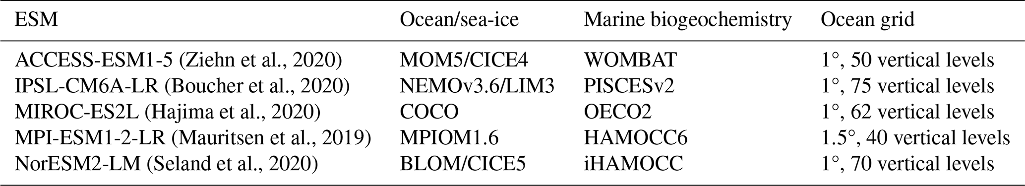
Eleven Earth system models (ESMs) provide the monthly 3D output fields required to compute AOU for the preindustrial control (piControl), historical and SSP5-8.5 future scenario simulations in a replica of the CMIP6 database. Among these eleven ESMs, only eight also provide outputs for the ideal-age tracer: MPI-ESM1.2-LR and MPI-ESM1.2-HR (Mauritsen et al., 2019), ACCESS-ESM1.5 (Ziehn et al., 2020), IPSL-CM6A-LR (Boucher et al., 2020), MIROC-ES2L (Hajima et al., 2020), NorESM2-LM and NorESM2-MM (Seland et al., 2020) and CanESM5 (Swart et al., 2019). The ideal-age tracer measures the time elapsed since a water parcel was last at the ocean surface. It is carried by the simulated ocean circulation and mixing. We use the ideal-age tracer to estimate the ventilation age of the ESMs. We do not consider NorESM2-MM and MPI-ESM1.2-HR here to keep only one variant of each model. We also do not consider CanESM5 because it does not provide phosphate fields that are used to compute the PO-tracer (Broecker et al., 1991), required to define water-masses (see Sect. 2.3). Hence, five ESMs (Table 1) are selected to be analysed in detail in this work. For comparison, we also compute AOU for the four remaining ESMs (CanESM5, CNRM-ESM2-1, Séférian et al., 2019, GFDL-ESM4, Dunne et al., 2020, UKESM1-0-LL, Sellar et al., 2020).

(Ziehn et al., 2020)(Boucher et al., 2020)(Hajima et al., 2020)(Mauritsen et al., 2019)(Seland et al., 2020)

Table 1 The CMIP6 Earth system models analysed in this study, their ocean, sea-ice and marine biogeochemistry, and their ocean grid resolution.

To have an observational baseline over the recent period, we also conduct an observation-based analysis of the trends in AOU and trends in ventilation age using the observational data product GLODAPv2 (2016) (Key et al., 2015; Olsen et al., 2016). We use temperature, salinity, phosphate and oxygen measurements. AOU is computed in the same way as for the ESMs (Sect. 2.2). We use the ventilation age product from Jeansson et al. (2021). In this product, measurements of the chlorofluorocarbon CFC-12 from GLODAPv2 (2016) are used with the transit time distribution (TTD) method to compute ventilation age, assuming 100 % saturation and a balance between advection and mixing, i.e. $\mathrm{\Delta }/\mathrm{\Gamma }=\mathrm{1}$. We only use data points where measurements of all variables mentioned are available. In order to be consistent with the ventilation age product, we opted for GLODAPv2 (2016), although more recent versions of the observational data product are available (e.g. Lauvset et al., 2024). The time range of the observational baseline is limited by the ventilation age dataset and extends from 1982 to 2013. Only observations below 1000 m are considered to avoid the influence of mixed-layer processes and subtropical gyres.

2.2 Apparent oxygen utilisation and remineralised carbon

Apparent oxygen utilisation (AOU in mol O₂ m⁻³) is computed as:

$$\begin{array}{}\text{(1)}& \text{AOU}={{\mathrm{O}}_{\mathrm{2}}}^{\text{sat}}-{\mathrm{O}}_{\mathrm{2}}\end{array}$$

where O₂ is the in-situ dissolved oxygen concentration and ${{\mathrm{O}}_{\mathrm{2}}}^{\text{sat}}$ is the dissolved oxygen concentration at saturation computed from temperature and salinity following Garcia and Gordon (1993, 1992). The amount of carbon resulting from this remineralisation (DIC_remin in g C m⁻³) is estimated as:

$$\begin{array}{}\text{(2)}& {\text{DIC}}_{\text{remin}}=m_{\mathrm{C}}\times R_{\mathrm{C}:{\mathrm{O}}_{\mathrm{2}}}\times \text{AOU}\end{array}$$

where m_C is the molecular weight of carbon (12.01 g mol⁻¹) and $R_{\mathrm{C}:{\mathrm{O}}_{\mathrm{2}}}$ is the stoichiometric ratio between carbon and oxygen (117 : 170, Anderson and Sarmiento, 1994).

Although providing a reasonably good indication of the BCP strength and its impact on atmospheric CO₂ (Koeve et al., 2020; Frenger et al., 2024), AOU has a couple of pitfalls that should be kept in mind. First, it assumes that at the surface, oxygen concentration is in equilibrium with the atmosphere. This assumption is valid in most of the ocean, yet in high latitudes, water parcels can be detrained from the mixed layer while being under-saturated leading to an overestimation of respiration and AOU, notably in the deep ocean (Ito et al., 2004; Duteil et al., 2013). True Oxygen utilisation (Ito et al., 2004) or Evaluated Oxygen utilisation (Duteil et al., 2013) are intended to overcome this limitation. However, the computation of these variables requires additional tracers (e.g., preformed O₂, (Tjiputra et al., 2020)) that are not routinely available in the CMIP6 output database. Another limitation is that AOU only measures aerobic remineralisation. Yet, when oxygen levels are too low, anaerobic remineralisation will take place and use other oxidants (e.g., nitrate for denitrification) instead of oxygen. In the open ocean, denitrification typically occurs in suboxic waters, when oxygen concentrations drop below 5 µmol O₂ L⁻¹ (Keeling et al., 2010). Suboxic waters represent only 0.1 % of the contemporary ocean and are located in the upper 1000 m (Deutsch et al., 2011; Keeling et al., 2010). During the 21st century, suboxic volume may extend but is projected to not exceed 1 % of the ocean volume (Deutsch et al., 2011; Cocco et al., 2013; Fu et al., 2018).

2.3 Definition of water-masses

We aim to find a linear relationship between the spatial distribution of AOU trends and ventilation age trends that is representative for most of the deep ocean. From now on and unless specified otherwise, we define the deep ocean as the ocean below 1000 m. We assess the linear relationship within different water-masses of the deep ocean characterized with a combination of the PO-tracer (PO^*, Broecker et al., 1991) and density.

For the water-mass definition of the ESMs, neither density nor PO^* are standard outputs in the CMIP6 database so that we compute density with the Gibbs SeaWater (GSW) Oceanographic Toolbox of TEOS-10 in xarray (Caneill and Barna, 2024; McDougall and Barker, 2011) and PO^* based on the definition by Broecker et al. (1991) (${\mathrm{PO}}^{*}={\mathrm{PO}}_{\mathrm{4}}+{\mathrm{O}}_{\mathrm{2}}/\mathrm{175}-\mathrm{1.95}$ µmol PO₄ kg⁻¹). Both variables are averaged over the years 1982 to 2013, i.e., the time period covered by the observational dataset used in this work. Our water-mass definition for the ESMs focuses only on the deep ocean and uses PO^*-thresholds to define water-masses originating in the North Atlantic and Southern Ocean. Broecker et al. (1998) state that the global distribution of PO^* has its minimum in the North Atlantic, its maximum in Southern Ocean and that the PO^* distribution for deep waters formed in the North Atlantic is very distinct from the distribution for deep waters formed in the Southern Ocean. Based on these statements, we defined the PO^*-thresholds for deep ocean water-masses individually for each ESM, using PO^* averaged on 1982–2013 and applying the following approach: (i) We compute the 95th percentile of the PO^* distribution in the deep subpolar North Atlantic, between 40–60° N and 0–70° E. (ii) We compute the 5th percentile of the PO^* distribution in the deep Southern Ocean, south of 55° S. (iii) The PO^*-threshold is defined as the average between the aforementioned percentiles. We find that Atlantic water-masses have PO^* values below the threshold while Southern water-masses have PO^* values above the threshold (see Fig. A1). For the Southern water-masses, it is necessary to exclude grid-cells located north of 60° N as some Arctic Ocean grid-cells would otherwise be included without being continuously connected to the Southern Ocean. All longitudes are considered for the Southern water-masses. For the Atlantic water-masses, only grid-cells located east of the Drake passage, west of 30° E and south of 80° N are included to exclude grid-cells in the Pacific and Indian Oceans that fulfil the PO^*-threshold and to exclude grid-cells in the Arctic Ocean. In the Arctic Ocean, a linear relationship between AOU trends and ventilation age trends emerges but with a very different slope than the one found for the Atlantic water-masses: here, AOU trends seem to be much more sensitive to ventilation age trends (not shown). Since our focus is on identifying linear relationships representative for most of the deep global ocean, we decided to exclude the Arctic from the analysis. We split the Southern and Northern water-masses into half according to density (Table A1), leading to four water-masses: (i) the Atlantic light waters, (ii) the Atlantic dense waters, (iii) the Southern light waters, and (iv) the Southern dense waters. These four water-masses cover at least 70 % of the entire deep ocean, depending on the ESM (70 % for IPSL-CM6A-LR and at least 92 % for the other models). For each water-mass and each ESM we define a spatial mask (Fig. A2), which is used to identify grid points belonging to the same water-mass and compute the linear regression between trends in AOU and trends in ventilation age (Sect. 2.4). We keep the masks constant throughout the historical and SSP5-8.5 simulations as the masks show minimal sensitivity to the time period used for creating the PO^* and density fields (Figs. A2 and A3).

Similar to the definition of water-masses used for the ESMs, observational data points are classified into water-masses originating from the Southern Ocean and North Atlantic (Fig. A4) based on their PO^* values. Waters originating in the Southern Ocean are defined via $\mathrm{1.2}\le {\mathrm{PO}}^{*}\le \mathrm{2.0}$ µmol PO₄ kg⁻¹ and those originating in the North Atlantic Ocean via ${\mathrm{PO}}^{*}<\mathrm{1.2}$ µmol PO₄ kg⁻¹ with PO^*-thresholds based on Broecker et al. (1998). Most of the data points used in this work belong to the densest half of waters originating from the North Atlantic Ocean or the Southern Ocean (98 % and 75 % of the points respectively). They were therefore not further separated into light and dense waters. The water-masses will be referred to as Southern dense waters and North Atlantic dense waters to facilitate a meaningful comparison with their model counterparts and are most representative of the water-mass end members.

2.4 Relationship between trends in AOU and trends in ventilation age

Just as the relationship between AOU and ventilation age can be linear (Sulpis et al., 2023), one might expect that the trends in AOU and the trends in ventilation age can be linearly related. In this work we intend to express the trends in AOU $\left(\frac{\mathrm{d}\text{AOU}}{\mathrm{d}t}\right)$ via trends in ventilation age $\left(\frac{\mathrm{d}\text{age}}{\mathrm{d}t}\right)$, in each point X, as follows:

$$\begin{array}{}\text{(3)}& {\displaystyle \frac{\mathrm{d}\text{AOU}}{\mathrm{d}t}}\left(X\right)=S_{\mathrm{\Delta }\text{age}}^{\mathrm{\Delta }\text{AOU}}\times {\displaystyle \frac{\mathrm{d}\text{age}}{\mathrm{d}t}}\left(X\right)+B+\mathit{\epsilon }\left(X\right).\end{array}$$

We assess the linear relationship between spatial fields of AOU trends and ventilation age trends within the previously define water-masses using a linear regression (Virtanen et al., 2020). The slope of the linear regression is the sensitivity of AOU changes to ventilation age changes ($S_{\mathrm{\Delta }\text{age}}^{\mathrm{\Delta }\text{AOU}}$). The intercept of the linear regression, B, represents a spatial average of the changes in AOU when there is no change in ventilation age. ε(X) is the error of the linear regression in each point. All together, B+ε represents the change in AOU that is not linearly related to changes in ventilation age, e.g. changes in remineralisation rates. $S_{\mathrm{\Delta }\text{age}}^{\mathrm{\Delta }\text{AOU}}$ defined here is connected to the oxygen utilisation rate (OUR) defined in other studies (e.g. Sulpis et al., 2023; Guo et al., 2023; Sonnerup et al., 2015; Feely et al., 2004; Sarmiento et al., 1990; Jenkins, 1982). Indeed, if the equation $\text{AOU}=\text{OUR}\times \text{age}$ is differentiated with respect to time, then $S_{\mathrm{\Delta }\text{age}}^{\mathrm{\Delta }\text{AOU}}$ and OUR are a similar quantity: an estimate of a spatio-temporal average of the local instantaneous oxygen utilisation rate. We choose to call the slope of the linear regression $S_{\mathrm{\Delta }\text{age}}^{\mathrm{\Delta }\text{AOU}}$ instead of OUR for two reasons: (1) we think this word conveys more accurately the purpose of the analysis, i.e., our investigation of the relationship between AOU trends and ventilation age trends and (2) we want to avoid ambiguity with studies estimating OUR using AOU and ventilation age (e.g., Sulpis et al., 2023; Guo et al., 2023; Sonnerup et al., 2015; Feely et al., 2004; Sarmiento et al., 1990; Jenkins, 1982) and not their temporal trends.

For the analysis of the ESMs, it is crucial to estimate and remove the drift in the simulated fields of AOU and ventilation age tracer before calculating their respective trends. The drifts are estimated for every ocean grid-cell of the ESMs using a linear regression over 250 years of the piControl simulation, starting from the year in the piControl simulation where the historical simulation has been initialised (Table A2). Outputs from the historical and SSP5-8.5 simulations are then drift corrected for each point in time t ($X_{\text{drift-corrected}}\left(t\right)=X_{\text{drift-uncorrected}}\left(t\right)-(t-t_{\mathrm{0}})\times \text{drift}$, with t₀ referring to 1850) before computing the trends. The trends are computed using a linear regression over the years (i) 1982–2013 of the historical simulation to match the time period of available observational data and (ii) 2015–2099 (the entire SSP5-8.5 simulation). When considering the ESMs, for the time period 1982–2013, between 49 % (NorESM2-LM) and 72 % (IPSL-CM6A-LR, MIROC-ES2L) of the deep ocean grid points have significant trends (p-value≤0.05) in both AOU and ventilation age, while between 84 % (NorESM2-LM) and 94 % (MIROC-ES2L) have significant trends for the time-period 2015–2099 (Fig. A5). The non-significant trends are very close to zero. For each ESM, we only consider grid-points with significant trends for computing the linear regression in each water-mass.

To overcome the difficulty of identifying trends with highly spatio-temporally sparse observational data, as it is the case for ventilation age estimates, we collapse the available observations in temperature-salinity (T-S) space. Trends in AOU and ventilation age are computed within bins in the T-S space (Fig. A6). To ensure that data points are geographically close to each other within each T-S bin, we (i) remove outliers defined as data points geographically further than twice the median distance to the median location and (ii) only keep points that are within a maximum distance from the median location (recomputed without the outliers). Thus the computation of the trends depends on two choices: the temperature and salinity resolution for the T-S bins and the maximum distance from the median location within each T-S bins. These choices affect: (i) the grouping of comparable measurements into the same T-S bin, regardless of their geographical location, (ii) the number of data points per T-S bin needed to identify significant trends (p-value≤0.05), and (iii) the number of trend estimates (one per T-S bin) required to establish a significant (p-value≤0.05) correlation between AOU trends and ventilation age trends. Trends for AOU and ventilation age, ($\mathrm{d}\text{AOU}/\mathrm{d}t$) and ($\mathrm{d}\text{age}/\mathrm{d}t$) are computed when five or more observations are grouped into a given T-S bin. Due to the substantial influence of the T-S bin size and the maximum distance, we conduct the analysis of the observational data 625 times with different random choices of these parameters to derive a distribution of the observation-based $S_{\mathrm{\Delta }\text{age}}^{\mathrm{\Delta }\text{AOU}}$. Temperature/salinity resolutions ranged from 0.026 to 0.325 °C and 0.0024 to 0.03, while maximum distance from 500 to 5000 km. Trends are then grouped into the Southern and Atlantic water-masses defined previously. Finally, as in the modelling counterpart of the analysis, a linear regression is computed between the spatial distributions of AOU trends and the ventilation age trends.

In this work we apply linear regressions for estimating trends and evaluating linear relationships. Further, we evaluate the significance of the trends and the linear relationship base on the p-values testing the null hypothesis of zero slopes, i.e. no trends or no linear relationship. When the p-value is lower than or equal to 0.05 we consider the trends or the linear relationship to be significant. The linear regression also provides a 95 % confidence interval for the slope, serving as a measure of the uncertainty associated with $S_{\mathrm{\Delta }\text{age}}^{\mathrm{\Delta }\text{AOU}}$. If this uncertainty is not specifically stated, it means that it is negligible with respect to the number of significant figures provided.

2.5 Evaluation of model-observation comparability

The analytical approach applied to observational data differs from the one applied to model outputs in three ways. (1) For the observational data, ventilation age is estimated using the TTD method with measurements of CFC-12. This method compares measured CFC-12 concentrations in the ocean with the evolution of CFC-12 concentrations in the atmosphere, assuming some balance between mixing and advection in ocean circulation. ESMs estimate the ventilation age via the ideal-age tracer, which counts the elapsed time since the last contact with the ocean surface. Hereafter, where necessary, we will distinguish between “ideal-age” and “TTD-mean-age”, the latter referring to age estimates derived from CFC-12. Where no distinction between the two is necessary, we will simply refer to “ventilation age”. (2) Observational datasets suffer from sparse and heterogeneous sampling in space and time, whereas ESM model results cover the entire ocean on a regular grid with monthly frequency. (3) Because the number of observational data is limited, trends must be computed within T-S bins while the outputs from ESMs gives time series for each grid-point.

We quantify the uncertainties in $S_{\mathrm{\Delta }\text{age}}^{\mathrm{\Delta }\text{AOU}}$ estimates derived from the observational dataset related to the aforementioned limitations using outputs from the NorESM2-LM historical simulation. We run two analysis:

• In TTD-UNC we quantify the uncertainties related to using the TTD method. To do so, we applied the TTD method to CFC-12 outputs from NorESM2-LM. Then, similar to the analysis of the ESMs ensemble (Sect. 2.4), (i) we compute trends in TTD-mean-age, (ii) we identify a linear relationship between the spatial fields of AOU trends and TTD-mean-age trends in the Atlantic dense and Southern dense water-masses and (iii) we derive $S_{\mathrm{\Delta }\text{age}}^{\mathrm{\Delta }\text{AOU}}$ values. In NorESM2-LM simulations, CFC-12 only partially invaded the ocean; e.g. most of the Pacific and Indian Oceans north of 40° S have CFC-12 concentration too small to derive a TTD-mean-age. Thus, in this analysis, we also sample the ideal-age outputs based on the spatio-temporal distribution of TTD-mean-age and derive reference values of $S_{\mathrm{\Delta }\text{age}}^{\mathrm{\Delta }\text{AOU}}$ using this ideal-age sample for the Atlantic dense and Southern dense water-masses. $S_{\mathrm{\Delta }\text{age}}^{\mathrm{\Delta }\text{AOU}}$ values derived from TTD-mean-age is compared against the reference $S_{\mathrm{\Delta }\text{age}}^{\mathrm{\Delta }\text{AOU}}$ values derived from ideal-age to quantify the uncertainty due to the TTD method.

• In SAMPLE-UNC, we quantify uncertainties due to data scarcity and the necessity to compute trends in T-S bins. We sample in space and time the NorESM2-LM outputs based on the observational data and replicate the analysis applied to the observational datasets, i.e. trends computed in T-S bins with the same 625 choices for T-S bins sizes and maximum distance that were used for the analysis of the observational dataset. The comparison between the obtained distribution of $S_{\mathrm{\Delta }\text{age}}^{\mathrm{\Delta }\text{AOU}}$ and the original $S_{\mathrm{\Delta }\text{age}}^{\mathrm{\Delta }\text{AOU}}$ values (no sampling, trends computed in each grid-point) quantifies the uncertainty of the T-S bins approach as well as of the data scarcity.

3 Results

3.1 Contemporary and future AOU across Earth system models

Contemporary spatial AOU patterns reflect physical transport and biological oxygen consumption. For example, AOU is particularly high in areas combining weak ventilation or ventilation of oxygen-depleted water-masses and intense remineralisation such as the deep ocean, the North Pacific or in the upper 1000 m in the equatorial band (Fig. 1a–c). Earth system models (ESMs) reproduce the general patterns shown by gap-filled observational products from the World Ocean Atlas 2023 (Fig. A7), yet with some regional strong positive and negative biases relative to observations (Fig. 1d–f). On average, ESMs overestimate AOU in the ocean deeper than 2000 m north of ca. 40° S and below 1000 m in the Pacific north of ca. 50° S. In contrast, ESMs underestimate AOU in the Southern Ocean (south of ca. 30° S) and above 1000 m in the northern hemisphere. In addition to biases in the model-mean, we note that there is a strong inter-model spread in large parts of the ocean, where the range of ESM values is higher than 70 % of the observation value (stippling in Figs. 1d–f and A8).

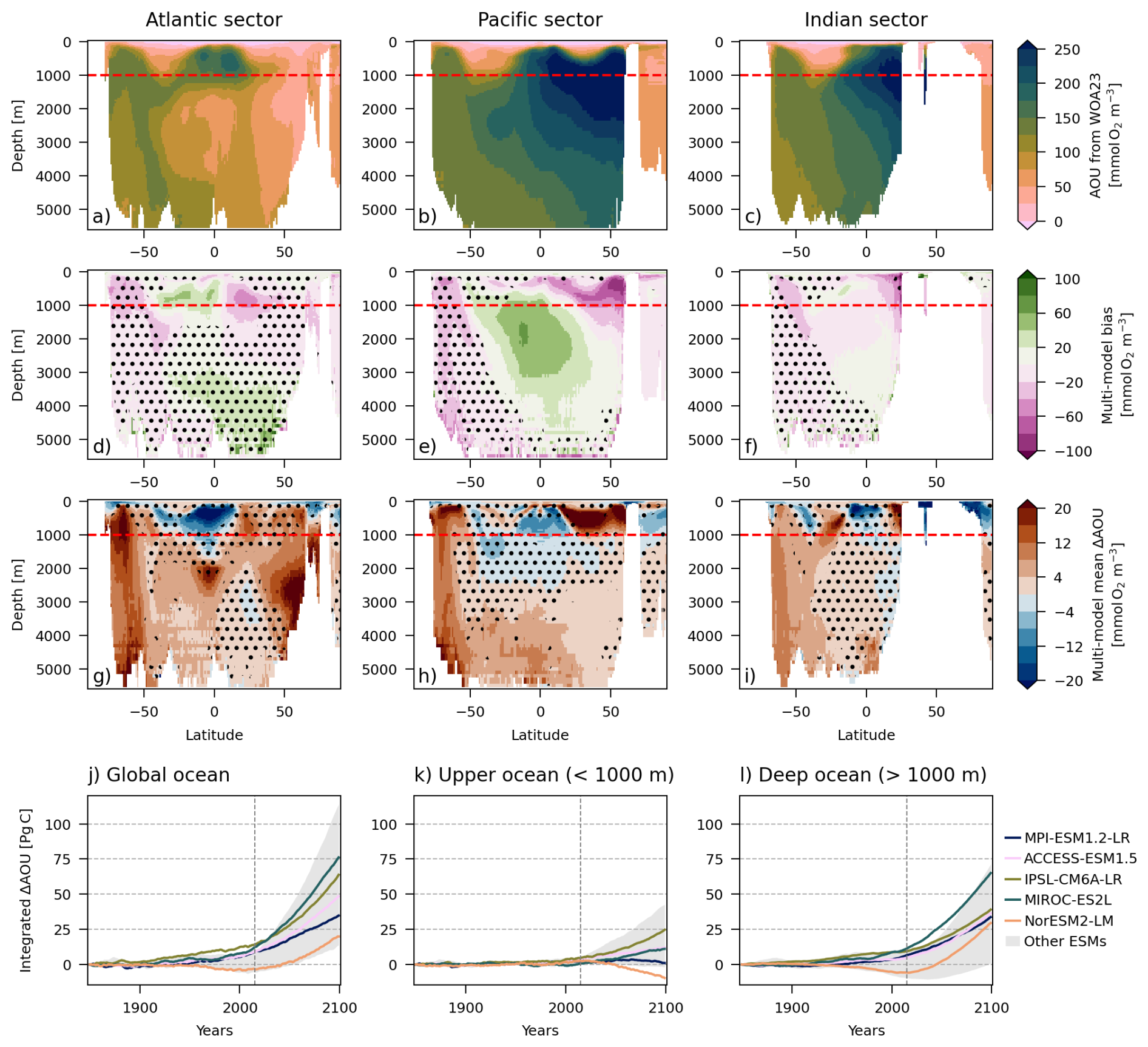
Figure 1 Evaluation of the simulated AOU and consistency in the projected change (ΔAOU). (a–c) AOU from the World Ocean Atlas 2023 (WOA23, Garcia et al., 2024), averaged over 1971–2000 in the Atlantic (10 to 60° W), Pacific (130 to 180° W) and Indian (40 to 90° E) sectors. (d–f) Multi-model mean of AOU bias against WOA23. Stippling shows AOU uncertainty in ESMs, i.e. when the range between the highest and lowest ESM values is greater than 70 % of the WOA23 value. Refer to Fig. A8 for individual ESM bias. (g–i) Multi-model mean of projected change (2070–2099 minus 1971–2000) under the SSP5-8.5 scenario, zonally average. Stippling shows ΔAOU uncertainty in ESMs, i.e. when the range between the strongest and weakest ΔAOU exceed three times the multi-model mean ΔAOU. Refer to Fig. A9 for individual ESM ΔAOU. The red dashed lines indicate the 1000 m separating the upper and deep ocean. (j–l) Time series of ΔAOU integrated on the (j) global, (k) upper and (l) deep ocean for each ESM considered in this study. The gray shading shows the range of other ESMs not used in this study (CanESM5, CNRM-ESM2-1, GFDL-ESM4, UKESM1-0-LL). The vertical dashed gray line (year 2015) separates the historical and SSP5-8.5 scenarios.

In the majority of the ocean, AOU is projected to increase under the SSP5-8.5 scenario (Fig. 1g–i). Most of the increase occurs below 1000 m (Fig. 1l), with agreement on the sign of change among the models (Fig. A9). Above 1000 m, AOU is projected to decrease in areas around the Equator or near the surface in the high latitude (Fig. 1g–i). The uncertainty of the projected change is considerable between ESMs with the inter-model spread exceeding three times the multi-model mean in the intermediate depth of the Pacific, in the low-latitude Indian, and in the deep subtropical North Atlantic (stippling in Figs. 1g–i and A9). By 2099, the integrated projected global change in AOU compared to 1850 ranges from 20 to 76 Pg C (Fig. 1j). A substantial share of the inter-model uncertainty in AOU changes stems from the deep ocean (below 1000 m). Here, the ESM spread encompasses 20 to 65 Pg C (Fig. 1l), while it ranges from −10 to 25 Pg C above 1000 m (Fig. 1k). The inter-model differences in AOU changes within the ESMs used in this study is representative of the inter-model differences in the AOU changes as seen by other ESMs (grey shading in Fig. 1j–l).

3.2 $S_{\mathrm{\Delta }\text{age}}^{\mathrm{\Delta }\text{AOU}}$ across Earth system models

For our model ensemble and the grid-points with significant trends in AOU and ideal-age in our defined Atlantic and Southern water-masses, the AOU trends are significantly correlated with the ideal-age trends for the years 1982–2013 (Figs. 2 and A10) and 2015–2099 (Fig. A11). When ideal-age increases or decreases due to changes in ventilation rates or redistribution of waters, AOU increases or decreases, respectively. In at least four out of five ESMs, spatial variability in ideal-age trends can explain more that half of the spatial variability in AOU trends in all four water-masses for the contemporary period, i.e. the coefficient of determination R² is higher than 0.5. Weaker correlations are potentially related to significant contribution of mixing over advection, spatial variability or local changes of respiration rate, or a partially inappropriate definition of water-masses. For example, in MPI-ESM1.2-LR, some of the grid-points included in the Atlantic light waters could be included in the Atlantic dense waters. Indeed, these grid points have densities very close to the median, their depths are comparable to those of Atlantic dense waters and they exhibit a linear relationship more similar to the one in Atlantic dense waters. For IPSL-CM6A-LR, in some grid-points of the Atlantic dense waters ideal-age unexpectedly increases while AOU decreases. These grid points, located in the Nordic Seas at approximately 3000 m depth, may have a different history compared to other Atlantic waters and thus would require a separate definition for their water-mass. In most ESMs, the correlation between AOU and ideal-age trends is weaker in the future period for all water-masses except the Southern dense waters, as indicated by the red vertical dashes in Fig. 3 (refer also to Fig. A14). Hence, ideal-age contributes less to the spatial variability of AOU. Depending on the ESM, our analysis covers only between 43 % and 66 % of the deep ocean for the 1982–2013 period, because (i) we only consider grid points with significant trends in ideal-age and AOU, and (ii) large part of the deep ocean have weak and non-significant trends during the contemporary period. For the 2015–2099 period, the linear regression analysis covers between 65 % and 94 % of the deep ocean, as the trends are stronger and more significant (Figs. A11 and A5). The inclusion of the non-significant trends decreases R² but does not substantially alter the slope of the linear regression (Figs. A12 and A13).

Figure 2 Distribution of the trends in ideal-age and trends in AOU for the contemporary period (1982–2013) simulated with five ESMs: (a) MPI-ESM1.2-LR, (b) ACCESS-ESM1.5, (c) IPSL-CM6A-LR, (d) MIROC-ES2L, (e) NorESM2-LM. The blue shading shows the number of data point for each bin of ideal-age trends and AOU trends for the Southern and Atlantic light/dense waters, accounting only for grid-points where ideal-age and AOU trends are significant. A linear regression is computed between the AOU trends and ideal-age trends for each water-mass. On each panel, the slope ($S_{\mathrm{\Delta }\text{age}}^{\mathrm{\Delta }\text{AOU}}$), the coefficient of determination (R²) and the fraction of the deep ocean volume are shown in different colours for each water-mass. The gray shading show the distribution of trends for the entire ocean.

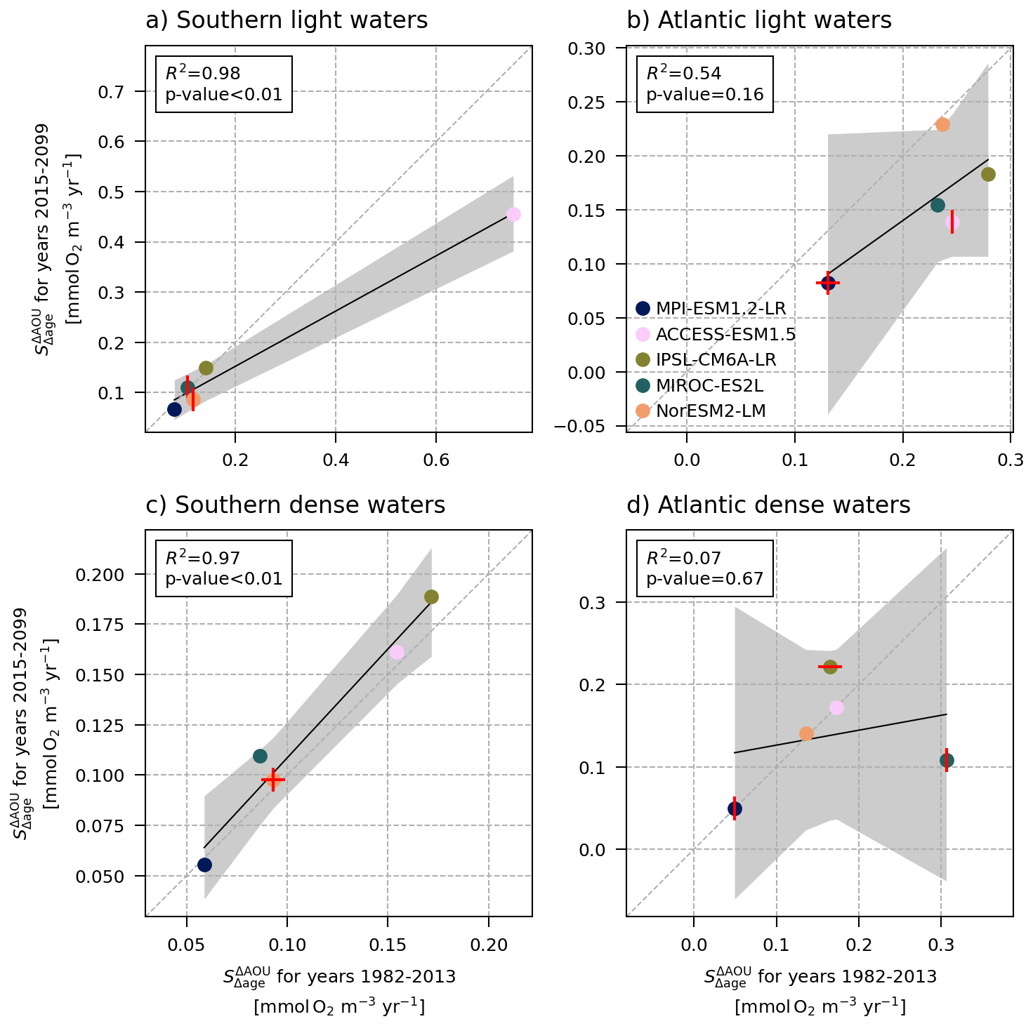
Figure 3 Distribution of the sensitivity of AOU change to ideal-age change ($S_{\mathrm{\Delta }\text{age}}^{\mathrm{\Delta }\text{AOU}}$) in each water-mass: (a) Southern light, (b) Atlantic light, (c) Southern dense, and (d) Atlantic dense. Each dot shows the $S_{\mathrm{\Delta }\text{age}}^{\mathrm{\Delta }\text{AOU}}$ for one ESM on the contemporary (1982–2013) and future (2015–2099) period. For few models, the red horizontal/vertical dash indicates a weak correlation (R²<0.5) between AOU trends and ideal-age trends for the contemporary/future period. The black line shows the linear regression and the gray shading its confidence interval. The associated coefficient of determination (R²) and the p-value are indicated in each panel. The diagonal dashed gray line is the 1:1 line.

The simulated sensitivities of AOU change to ideal-age change ($S_{\mathrm{\Delta }\text{age}}^{\mathrm{\Delta }\text{AOU}}$) are relatively similar for both light and dense waters. Yet, $S_{\mathrm{\Delta }\text{age}}^{\mathrm{\Delta }\text{AOU}}$ is slightly stronger in light waters, likely due to stronger remineralisation in the shallower regions. Within each water-mass, $S_{\mathrm{\Delta }\text{age}}^{\mathrm{\Delta }\text{AOU}}$ varies substantially, increasing by at least a factor of two between the least and the most sensitive ESM. We find that ESMs with a large (small) $S_{\mathrm{\Delta }\text{age}}^{\mathrm{\Delta }\text{AOU}}$ in the contemporary period (1982–2013) also have a large (small) $S_{\mathrm{\Delta }\text{age}}^{\mathrm{\Delta }\text{AOU}}$ for the future period under the high CO₂ future scenario SSP5-8.5 (Fig. 3). The linear relation between present and future $S_{\mathrm{\Delta }\text{age}}^{\mathrm{\Delta }\text{AOU}}$ is strong for the Southern waters across our model ensemble, as indicated by the linear regression giving coefficients of determination higher than 0.97 and p-values below 0.01 (Fig. 3). In the Atlantic waters, the linear relationship is not significant (p-value>0.05), mostly due to the distinct behaviour of two models. Specifically, $S_{\mathrm{\Delta }\text{age}}^{\mathrm{\Delta }\text{AOU}}$ in NorESM2-LM does not decline in the future period for Atlantic light waters, and $S_{\mathrm{\Delta }\text{age}}^{\mathrm{\Delta }\text{AOU}}$ in MIROC-ES2L shows a substantial decrease in the future period for Atlantic dense waters.

Once a linear relationship has been established providing the average trend in AOU for a given trend in ideal-age, we can use it to further quantify the contribution of ideal-age trends to the trends in AOU in each ESM. This contribution is estimated by multiplying the ideal-age trends with $S_{\mathrm{\Delta }\text{age}}^{\mathrm{\Delta }\text{AOU}}$ for each of the four water-masses ($S_{\mathrm{\Delta }\text{age}}^{\mathrm{\Delta }\text{AOU}}\times \frac{\mathrm{d}\text{age}}{\mathrm{d}t}$ in Eq. 3). Globally integrated, ideal-age trends contribute between 43 % (ACCESM-ESM1.5) and 106 % (IPSL-CM6A-LR) to the AOU trends in these water-masses (Fig. 4). The disparities in the contributions of ideal-age trends across models arise from differences in the both the ideal-age trends themselves and in $S_{\mathrm{\Delta }\text{age}}^{\mathrm{\Delta }\text{AOU}}$. MPI-ESM1.2-LR and ACCESS-ESM1.5 are the two models with the lowest contributions of ideal-age trends but for different reasons: MPI-ESM1.2-LR has the lowest $S_{\mathrm{\Delta }\text{age}}^{\mathrm{\Delta }\text{AOU}}$ and relatively strong ideal-age trends, while ACCESS-ESM1.5 has high $S_{\mathrm{\Delta }\text{age}}^{\mathrm{\Delta }\text{AOU}}$ and weak ideal-age trends. In contrast to these two models with compensating $S_{\mathrm{\Delta }\text{age}}^{\mathrm{\Delta }\text{AOU}}$ and ideal-age trends, MIROC-ES2L shows both a high $S_{\mathrm{\Delta }\text{age}}^{\mathrm{\Delta }\text{AOU}}$ and strong ideal-age trends. This combination leads to MIROC-ESL having the highest contribution of ideal-age trends to AOU trends.

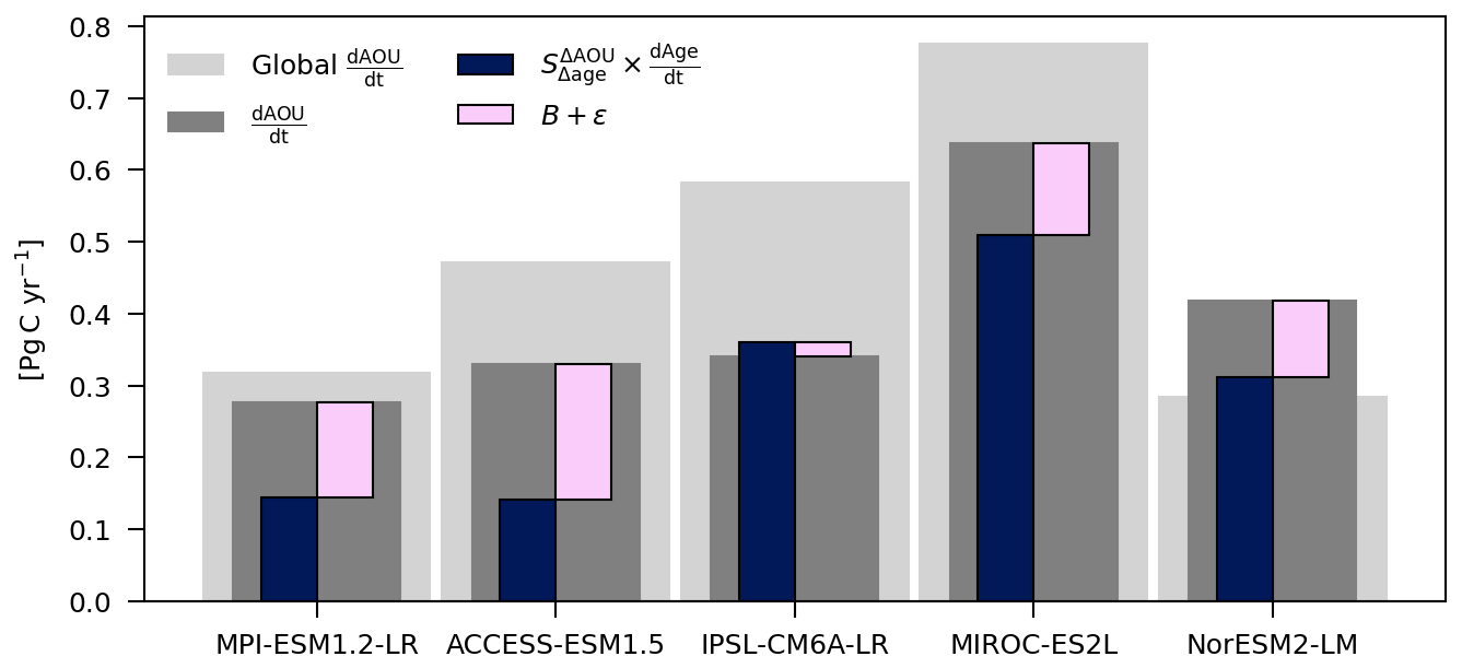
Figure 4 Spatially integrated trends in AOU ($\frac{\mathrm{d}\text{AOU}}{\mathrm{d}t}$, dark and light grey) and the contribution from trends in ideal-age $\left(S_{\mathrm{\Delta }\text{age}}^{\mathrm{\Delta }\text{AOU}}\times \frac{\mathrm{d}\text{age}}{\mathrm{d}t}\right),\text{dark blue}$ under the SSP5-8.5 climate change scenario simulated with five ESMs: MPI-ESM1.2-LR, ACCESS-ESM1.5, IPSL-CM6A-LR, MIROC-ES2L, NorESM2-LM. The remainder (B+ε, pink) is computed as the difference between the two aforementioned components (see Eq. 3). Shown are the trends integrated over the global ocean (light grey), and over the water-masses considered in this study. Trends are computed for the period from 2015 to 2099.

In general, the positive trends in AOU mostly arise from the Southern dense water-mass, and are driven by positive trends in ideal-age (Fig. 5). The Atlantic dense water-mass exhibits also intense local positive AOU trends driven by ideal-age trends. In these two ventilation regions, the models suggest a weakening in the ventilation rates in the future (increasing ideal-age). In contrast, negative AOU trends are mostly located in the Southern and Atlantic light water-masses, found between 1000 and 2000 m in the subtropics and equatorial region. In these areas, negative ideal-age trends play a major role indicating that waters get younger because of a shift in water-mass structure or stronger ventilation, though stronger ventilation seems less likely considering that stratification increase everywhere in the ocean in the future simulation (Kwiatkowski et al., 2020). Such distinction between light and dense water-masses have been previously identified for the contemporary period in the Nordic Seas (Jeansson et al., 2023). The remainder term, B+ε, locally either slightly compensates or reinforces changes driven by ideal-age trends, resulting globally in a positive contribution to AOU trends.

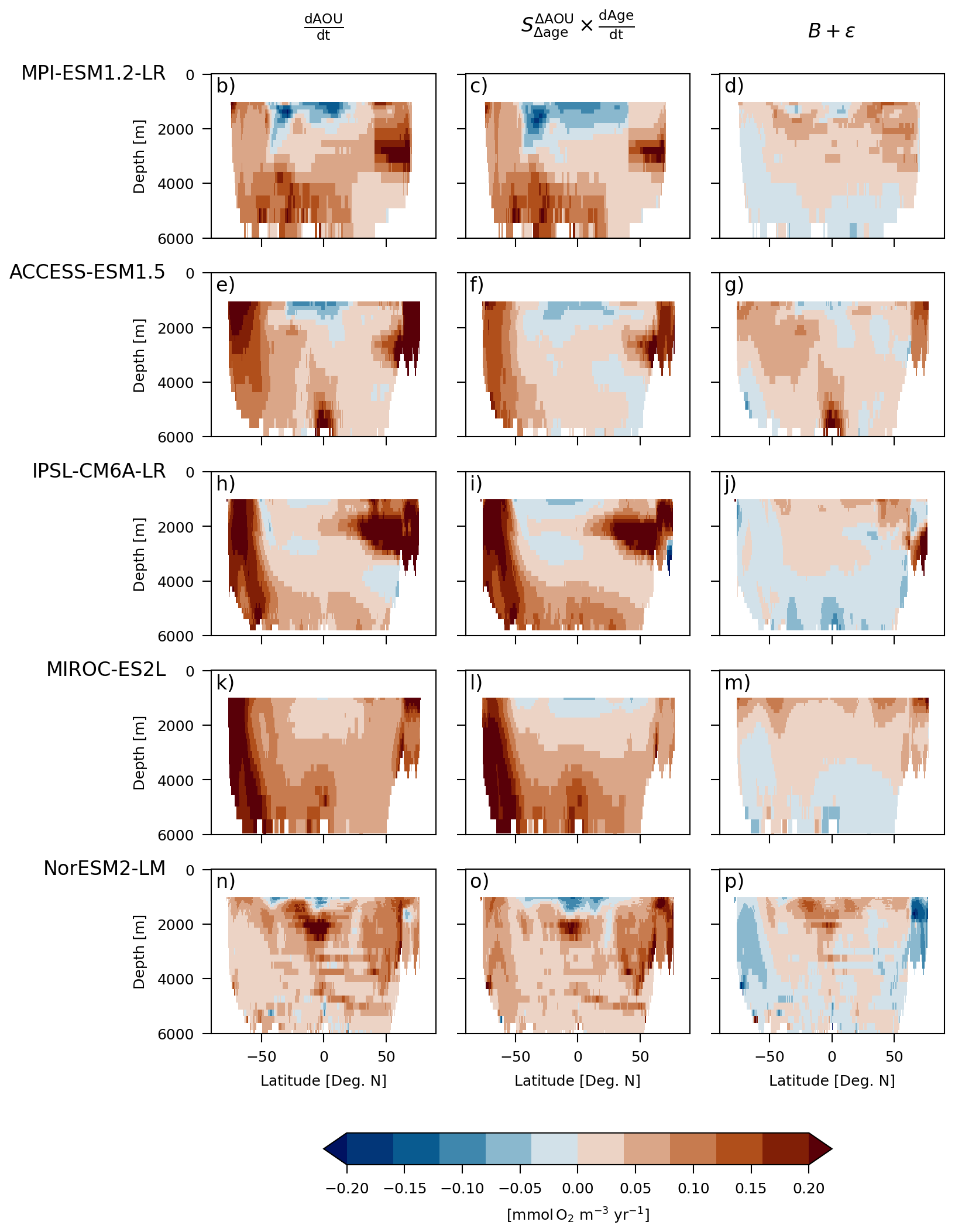
Figure 5 Zonally averaged trends in AOU ($\frac{\mathrm{d}\text{AOU}}{\mathrm{d}t}$, first column) and the contribution from trends in ideal-age ($S_{\mathrm{\Delta }\text{age}}^{\mathrm{\Delta }\text{AOU}}\times \frac{\mathrm{d}\text{age}}{\mathrm{d}t}$, second column) under the SSP5-8.5 climate change scenario simulated with five ESMs: MPI-ESM1.2-LR, ACCESS-ESM1.5, IPSL-CM6A-LR, MIROC-ES2L, NorESM2-LM. The remainder (B+ε, third column) is computed as the difference between the two aforementioned components (see Eq. 3). Trends are computed for the period from 2015 to 2099 and are zonally averaged on the four water-masses considered in this study, accounting only for grid points with significant trends (p-value>0.05).

3.3 $S_{\mathrm{\Delta }\text{age}}^{\mathrm{\Delta }\text{AOU}}$ from observational data

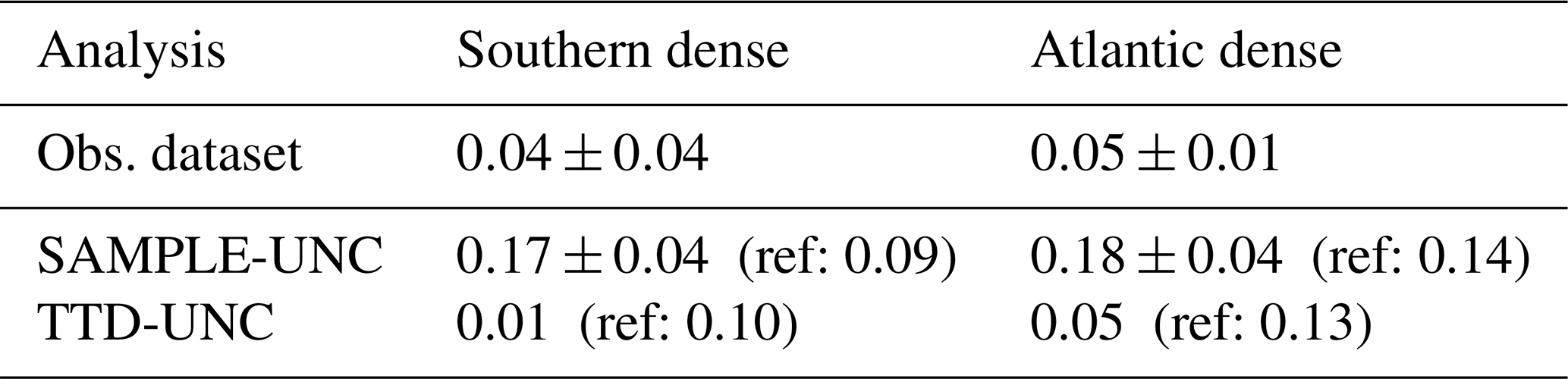
A positive linear correlation is also found between the significant trends in AOU and TTD-mean-age from the observation dataset (Fig. A15). $S_{\mathrm{\Delta }\text{age}}^{\mathrm{\Delta }\text{AOU}}$ evaluated from the observational dataset are 0.04 ± 0.04 and 0.05 ± 0.01 $\mathrm{mmol}{\mathrm{O}}_{\mathrm{2}}{\mathrm{m}}^{-\mathrm{3}}{\mathrm{yr}}^{-\mathrm{1}}$ for the Southern dense and Atlantic dense water-masses, respectively (Fig. A15). Here, the water-masses have not been split into light and dense waters due to the limited number of data points (see Sect. 2.3). For both water-masses, the coefficient of determination, R², varies between 0.2 and 1 depending on the methodological choices for the analysis, with higher R² values typically associated with higher $S_{\mathrm{\Delta }\text{age}}^{\mathrm{\Delta }\text{AOU}}$.

The scarcity of observational data and the use of the TTD-mean-age introduce uncertainties into the observation-based $S_{\mathrm{\Delta }\text{age}}^{\mathrm{\Delta }\text{AOU}}$. When the analysis is replicated with a sample of NorESM2-LM outputs (SAMPLE-UNC analysis, see Sect. 2.5), $S_{\mathrm{\Delta }\text{age}}^{\mathrm{\Delta }\text{AOU}}$ estimates are 0.17 ± 0.04 and 0.18 ± 0.04 $\mathrm{mmol}{\mathrm{O}}_{\mathrm{2}}{\mathrm{m}}^{-\mathrm{3}}{\mathrm{yr}}^{-\mathrm{1}}$, for the Southern dense and Atlantic dense water-masses, respectively (Table 2). This is an increase of 0.08 and 0.04 $\mathrm{mmol}{\mathrm{O}}_{\mathrm{2}}{\mathrm{m}}^{-\mathrm{3}}{\mathrm{yr}}^{-\mathrm{1}}$ when compared to the reference values (analysis with non-scarce data). Using trends in TTD-mean-age as an estimate of trends in ventilation age introduce further uncertainties in the estimate of $S_{\mathrm{\Delta }\text{age}}^{\mathrm{\Delta }\text{AOU}}$ from the observational dataset (TTD-UNC analysis, see Sect. 2.5). When computed with CFC-12 outputs from NorESM2-LM, trends in TTD-mean-age are generally much stronger than trends in ideal-age (not shown). In some instances, trends may even oppose each other. In consequence, $S_{\mathrm{\Delta }\text{age}}^{\mathrm{\Delta }\text{AOU}}$ derived from TTD-mean-age is 0.01 and 0.05 $\mathrm{mmol}{\mathrm{O}}_{\mathrm{2}}{\mathrm{m}}^{-\mathrm{3}}{\mathrm{yr}}^{-\mathrm{1}}$ for the Southern dense and Atlantic dense water-masses, respectively (Table 2). This is 0.09 and 0.08 $\mathrm{mmol}{\mathrm{O}}_{\mathrm{2}}{\mathrm{m}}^{-\mathrm{3}}{\mathrm{yr}}^{-\mathrm{1}}$ lower than the reference values ($S_{\mathrm{\Delta }\text{age}}^{\mathrm{\Delta }\text{AOU}}$ derived from ideal-age). Hence, using trends in TTD-mean-age lead to underestimation of observation-based $S_{\mathrm{\Delta }\text{age}}^{\mathrm{\Delta }\text{AOU}}$ while the scarcity of data points and the need to compute trends in the T-S space results in overestimating it. Together, these overestimation and underestimation compromise the comparability of observation-based $S_{\mathrm{\Delta }\text{age}}^{\mathrm{\Delta }\text{AOU}}$ with $S_{\mathrm{\Delta }\text{age}}^{\mathrm{\Delta }\text{AOU}}$ derived from the ESMs.

Table 2 Sensitivity of AOU trends to ventilation age trends ($S_{\mathrm{\Delta }\text{age}}^{\mathrm{\Delta }\text{AOU}}$ in $\mathrm{mmol}{\mathrm{O}}_{\mathrm{2}}{\mathrm{m}}^{-\mathrm{3}}{\mathrm{yr}}^{-\mathrm{1}}$) estimated from the observational dataset and the uncertainty analyses using NorESM2-LM outputs (SAMPLE-UNC and TTD-UNC). For the analysis of the observational dataset and SAMPLE-UNC, values are the mean ± one standard deviation of the $S_{\mathrm{\Delta }\text{age}}^{\mathrm{\Delta }\text{AOU}}$ distribution derived from the 625 analyses performed. The reference values in bracket are: for the SAMPLE-UNC analysis, $S_{\mathrm{\Delta }\text{age}}^{\mathrm{\Delta }\text{AOU}}$ computed with non-scarce data and, for the TTD-UNC analysis, $S_{\mathrm{\Delta }\text{age}}^{\mathrm{\Delta }\text{AOU}}$ derived using trends in ideal-age.

4 Discussion

Our results highlight the importance of ventilation changes on the changes in AOU and therefore on DIC_remin in the deep ocean. Previous studies suggested that circulation was the main driver of changes in interior carbon content during the past and future climate (Bopp et al., 2017; Kessler et al., 2018; Liu and Primeau, 2023). We quantify that between 2015 and 2099, under the SSP5-8.5 climate change scenario and in the ocean below 1000 m, a ventilation slow down contributes between 43 % and 106 % to the increase in DIC_remin. The densest water-mass coming from the Southern Ocean (southern dense water-mass) contribute predominantly to the deep ocean DIC_remin increase. This water-mass covers a large portion of the deep ocean, and have particularly strong correlation between spatial fields of AOU trends and ideal-age trends. While we highlight the importance of change in ideal-age in this water-mass, a substantial portion of the change in AOU is not driven by change in ideal-age in lighter water-masses. Here, changes in export (Henson et al., 2022), spatially variable oxygen utilisation rate (Sulpis et al., 2023) or changes in remineralisation with temperature (Brewer and Peltzer, 2017) can de-correlate changes in AOU from changes in ideal-age. Furthermore, in a transient climate, the conditions (strong advection over mixing and spatially even respiration) for a linear relationship between AOU trends and ventilation age trends can change over time. Changes in circulation can also recombine water-masses differently bringing in waters with varying histories; waters can follow different pathways and go through different respiration fields (Guo et al., 2023). In the lighter water-masses and in the Atlantic dense water-mass, changes in ideal-age explain a slightly smaller portion of the spatial variability of AOU changes in the future compare to the contemporary period (weaker R²), suggesting caution when interpreting ventilation changes from AOU.

Our work shows that ESMs have substantially different sensitivities of AOU to ventilation changes, indicating uncertainty. The models that simulate the strongest slow down of the overturning circulation do not necessarily produce the strongest increase in AOU (Liu et al., 2023), complicating the interpretation of projections of carbon sequestration. Divergent model sensitivities may reflect different remineralization rate parametrizations (Maerz et al., 2026; Brabson et al., 2026), different organic matter fluxes into the interior (Henson et al., 2022) and more generally differences in the representation of marine biogeochemistry (Séférian et al., 2020; Fennel et al., 2022). The inter-model spread in the sensitivities might also indicate model dependent spatial distribution of water-masses and the differences in ventilation mechanisms (mixing, advection) and pathways. Additionally, the AOU response could be state dependent, varying with the physical and biogeochemical background (e.g., stratification, export production, remineralization depth).

One of the initial motivation for this work was to constrain ESM projections of AOU using changes in ventilation age. Our results suggest that the constraining of deep ocean ventilation changes in ESMs with observed ventilation changes (Waugh et al., 2013; Gerke et al., 2024; Wefing et al., 2025; Guo et al., 2026) is a prerequisite for constraining projections of deep ocean AOU. However, identifying the best ESMs at projecting deep ocean ventilation changes is challenging. For instance, under a different climate, the last glacial maximum, ESMs simulate very different changes in Atlantic MOC (meridional overturning circulation) depth and strength, and no ESM is consistent with the estimations from proxies (Sherriff-Tadano and Klockmann, 2021). On the other hand, simulated changes in the North Atlantic circulation during stadial-interstadial climate transition show promising comparison with proxy data (Waelbroeck et al., 2023). An accurate projection of the carbon sequestration by the BCP in the deep ocean needs an accurate formation of the deep water-masses in the North Atlantic and Southern Ocean, yet it is not possible to determine even one CMIP6 model that represents those accurately (Heuzé, 2021).

Constraining only ventilation changes may not be enough to identify the best ESMs at projecting changes in AOU in the interior ocean, since the divergent sensitivities of AOU to ventilation changes modulate ventilation-driven changes in AOU. The linear relationship between present and future sensitivity across ESMs is promising, in particular in the Southern dense water-mass which covers the largest portion of the deep ocean. It can, in theory, be used to identify ESMs whose sensitivities are the most consistent with observations in the contemporary period and be used to constrain the sensitivity of the future period. However, at this point in time, we cannot directly constrain the sensitivity following an emergent constraint approach (Bourgeois et al., 2022; Kwiatkowski et al., 2017; Goris et al., 2023) because of the small ESM ensemble available and the uncertainties in the observations based estimates. Improved constraints using oxygen, transient tracers, and water-mass age diagnostics, alongside particle flux observations, can help evaluate and reduce structural model uncertainties (Marsay et al., 2015; DeVries and Primeau, 2011).

The reliability of the $S_{\mathrm{\Delta }\text{age}}^{\mathrm{\Delta }\text{AOU}}$ estimates from observational data is compromised by the limited number of data points and the usage of the TTD method for estimating ventilation age trends. While the scarcity of data and the need to compute trends in T-S space lead to a substantial overestimation when compared to a non-scarce data set, using trends in TTD-mean-age results in an equally strong underestimation when compared to trends computed with ideal-age. While we are confident in our estimate of the first uncertainty, we are more cautious regarding the evaluation of the second uncertainty (TTD method). In the model simulations, in the ocean below 1000 m, only the Southern Ocean and the North Atlantic are well-ventilated to the degree that the CFC-12 concentrations can provide TTD-mean-age estimates. Thus, we can evaluate trends in TTD-mean-age against trends in ideal-age only in these regions, representing a limited portion of the area covered by the observational dataset. Caution is warranted when using TTD-mean-age to assess changes in ventilation, especially when TTD methods depend on assumptions about the balance between advection and mixing ($\mathrm{\Delta }/\mathrm{\Gamma }$). $\mathrm{\Delta }/\mathrm{\Gamma }=\mathrm{1}$ is a good compromise for the entire ocean but regionally dependent $\mathrm{\Delta }/\mathrm{\Gamma }$ would lead to more optimal TTD-mean-age when compared to model (He et al., 2018). Approaches employing dual constraint are promising and should be further explored (Guo et al., 2025, 2026). While imperfect, the estimates of $S_{\mathrm{\Delta }\text{age}}^{\mathrm{\Delta }\text{AOU}}$ based on scarce observational data and TTD-mean-age remain the only viable option for comparing $S_{\mathrm{\Delta }\text{age}}^{\mathrm{\Delta }\text{AOU}}$ derived from ESMs. Given that $S_{\mathrm{\Delta }\text{age}}^{\mathrm{\Delta }\text{AOU}}$ is to some extent similar to an estimation of the oxygen utilisation rate averaged within the water-masses considered, comparison with prior observational-based OUR estimates is appropriate. In the deep ocean, oxygen utilisation rate estimations typically vary around 0.1 $\mathrm{mmol}{\mathrm{O}}_{\mathrm{2}}{\mathrm{m}}^{-\mathrm{3}}{\mathrm{yr}}^{-\mathrm{1}}$ (Sulpis et al., 2023), substantially higher than the observation-based estimates from our work, yet on the lower end of the $S_{\mathrm{\Delta }\text{age}}^{\mathrm{\Delta }\text{AOU}}$ range derived from ESMs.

One caveat of our work is the use of AOU as a proxy of remineralised organic matter, notably as we focus on the deep ocean where water parcels coming from the high latitude can be exported while being-undersaturated with respect to oxygen (Ito et al., 2004; Duteil et al., 2013). Interestingly, when compared to true oxygen utilisation (TOU), which is a more accurate measure of remineralised organic matter, AOU overestimates TOU but changes in AOU underestimates changes in TOU by 25 % (Koeve et al., 2020). This uncertainty is also linked to the the physical representation biases in ESMs that strongly affect the projections of interior oxygen changes (Ito et al., 2026), hence AOU. In addition, AOU underestimates organic matter remineralisation because it does not account for denitrification occurring in suboxic waters. In global warming simulations, the volume of suboxic waters increases all along the 20th and 21st century resulting in a small increase in denitrification (Fu et al., 2018; Cocco et al., 2013). Nevertheless, since suboxic waters are mostly located in the upper 1000 m of the ocean, the omission of denitrification is expected to have a minimal impact on our results. If it does have an impact, it would likely result in a small underestimation of $S_{\mathrm{\Delta }\text{age}}^{\mathrm{\Delta }\text{AOU}}$. Altogether, this highlights the need to consider the AOU uncertainty when inferred as a proxy for remineralised organic matter in ESMs, calling for getting TOU outputs in future Coupled Model Intercomparison Project in order to properly quantify the projected BCP changes.

5 Conclusions

Understanding changes in ocean BCP and its impact on future climate change remains an outstanding research question (Tjiputra et al., 2025). In this work, we have demonstrated that the spatial fields of AOU trends (an indicator of changes in the BCP) and ideal-age trends are correlated in the ocean deeper than 1000 m. Here, spatial variability in ideal-age trends can explain more than half of the spatial variability in AOU trends (R²≥0.5). This relationship is identified in simulations of the contemporary period (1982–2013) and simulations of the future period (2015–2099) under the SSP5-8.5 climate change scenario. The sensitivity of AOU change to ideal-age change, $S_{\mathrm{\Delta }\text{age}}^{\mathrm{\Delta }\text{AOU}}$ (that is, the slope of the linear regression), varies between the ESMs and the water-masses from 0.05 to 0.75 $\mathrm{mmol}{\mathrm{O}}_{\mathrm{2}}{\mathrm{m}}^{-\mathrm{3}}{\mathrm{yr}}^{-\mathrm{1}}$ for the contemporary period, depending on the ocean regions. $S_{\mathrm{\Delta }\text{age}}^{\mathrm{\Delta }\text{AOU}}$ remain relatively similar when computed for the 2015–2099 period. Using the linear relationship we estimate that, for the 2015–2099 time period, the increase in ideal-age, due to changes in ventilation rates or redistribution of waters, contribute between 43 % and 106 % to the increase in deep ocean DIC_remin, which varies between ESMs.

Disparities in deep ocean AOU changes across ESMs stem from differences in ventilation changes and differences in the sensitivity of AOU to these ventilation changes. Constraining deep ocean AOU changes requires addressing both ventilation changes and sensitivities. Constraining sensitivities seems in reach, but would require a greater number of models providing ideal-age and preformed tracers, as well as expanding the observational database and refining the estimation of ventilation age changes from ocean tracers. It is our hope that the ESMs represented in CMIP7 will offer further improvements compared to CMIP6 in terms of their representation of ventilation, especially deep water formation, as well as available outputs in the CMIP7 database. Given a larger model ensemble and more observations, our approach is a promising solution that would allow us to constrain the remineralised carbon sequestration in the deep ocean for the next ESM generations to come. Finally, while ventilation-driven changes in deep ocean carbon sequestration are substantial, they represent only one aspect of the overall process. Changes in biological processes also play a substantial role, particularly in shallower ocean regions. Uncertainties associated to the biological processes driving interior ocean remineralisation in the different models remain (Henson et al., 2024), deserving specific attention to understand carbon sequestration in the intermediate depth ocean. Last but not least, constraining simulated changes in oxygen utilisation will also be one step towards reconciling simulated and observed rates of current deoxygenation (Ito et al., 2026). Constraining models uncertainties is critical for reliable projections of coupled ocean carbon, and oxygen budgets under climate change.

Appendix A

Table A1 Range of the potential density anomaly in kg m⁻³ in each water-masses for the 1982–2013 period. The anomaly is relative to a reference pressure of 0 dbar. It is computed with the Gibbs SeaWater (GSW) Oceanographic Toolbox of TEOS-10 in xarray (Caneill and Barna, 2024; McDougall and Barker, 2011). The Southern and Atlantic water-masses are define based on the PO-tracer (PO^*, Broecker et al., 1991). Each of these two water-masses is then split into half according to the median of the density distribution. See the method section in the main manuscript for details.

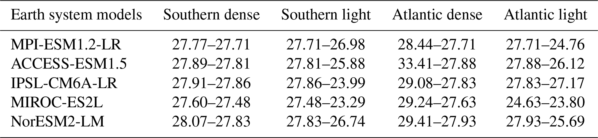
Table A2 Correspondence of years between the pre-industrial control simulation (pi-Control) and the historical and future projections simulations.

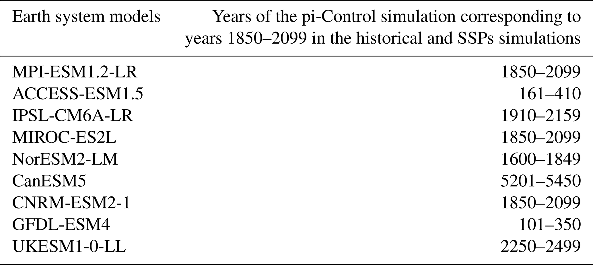
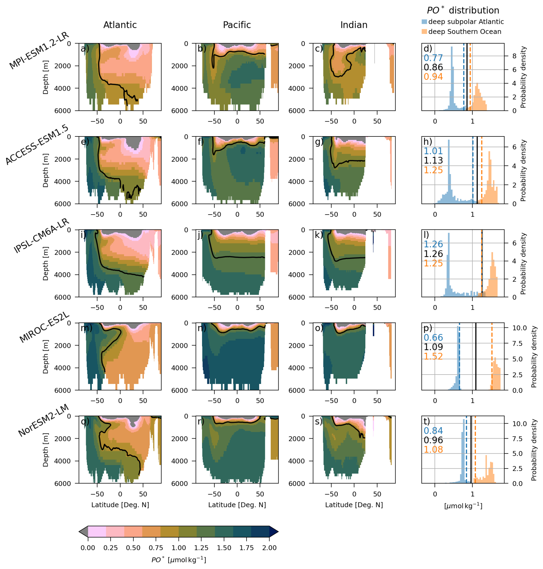
Figure A1 Contemporary (1982–2013) depth-latitude sections of PO-tracer (PO^*, Broecker et al., 1991) and its distributions in five ESMs: MPI-ESM1.2-LR, ACCESS-ESM1.5, IPSL-CM6A-LR, MIROC-ES2L, and NorESM2-LM – listed from top to bottom. In the 3 first column, PO^* values are zonally averaged across three ocean sectors: the Atlantic (10–60° W), the Pacific (130–180° W) and the Indian (40–90° E), organized from left to right. On the last column are shown the PO^* distributions in the deep subpolar North Atlantic and the deep Southern ocean (see methods) with the dashed vertical lines showing the 95th and 5th percentile, respectively to each distribution. The black plain lines show the average between the percentile and is also indicated as a black contour line on the depth-latitude sections. The coloured numbers indicate the respective values.

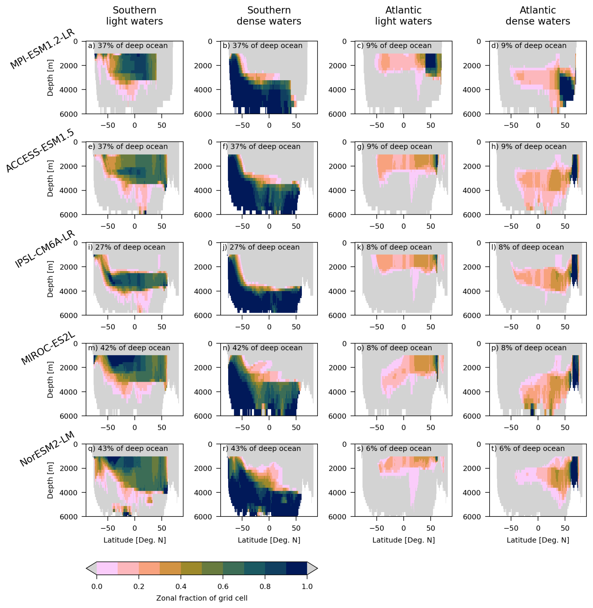
Figure A2 Distribution of the four water-masses – Southern light, Southern dense, Atlantic light, Atlantic dense, from left to right – in the five ESMs: MPI-ESM1.2-LR, ACCESS-ESM1.5, IPSL-CM6A-LR, MIROC-ES2L, NorESM2-LM, arranged from top to bottom. Each depth-latitude sections represent the zonal fraction of grid-cell belonging to the water-mass. For instance, one indicates that all the grid cells zonally belong to the water-mass, while 0.5 indicates that half of the grid cells zonally belong to the water-mass. Areas in grey depict regions where no grid cells are assigned to the water-mass. Percentages indicate the fraction of the deep ocean volume covered by each water-mass. The water-masses are defined using PO-tracer and density fields averaged over the 1982–2013 period (refer to the methods section in the main manuscript for details).

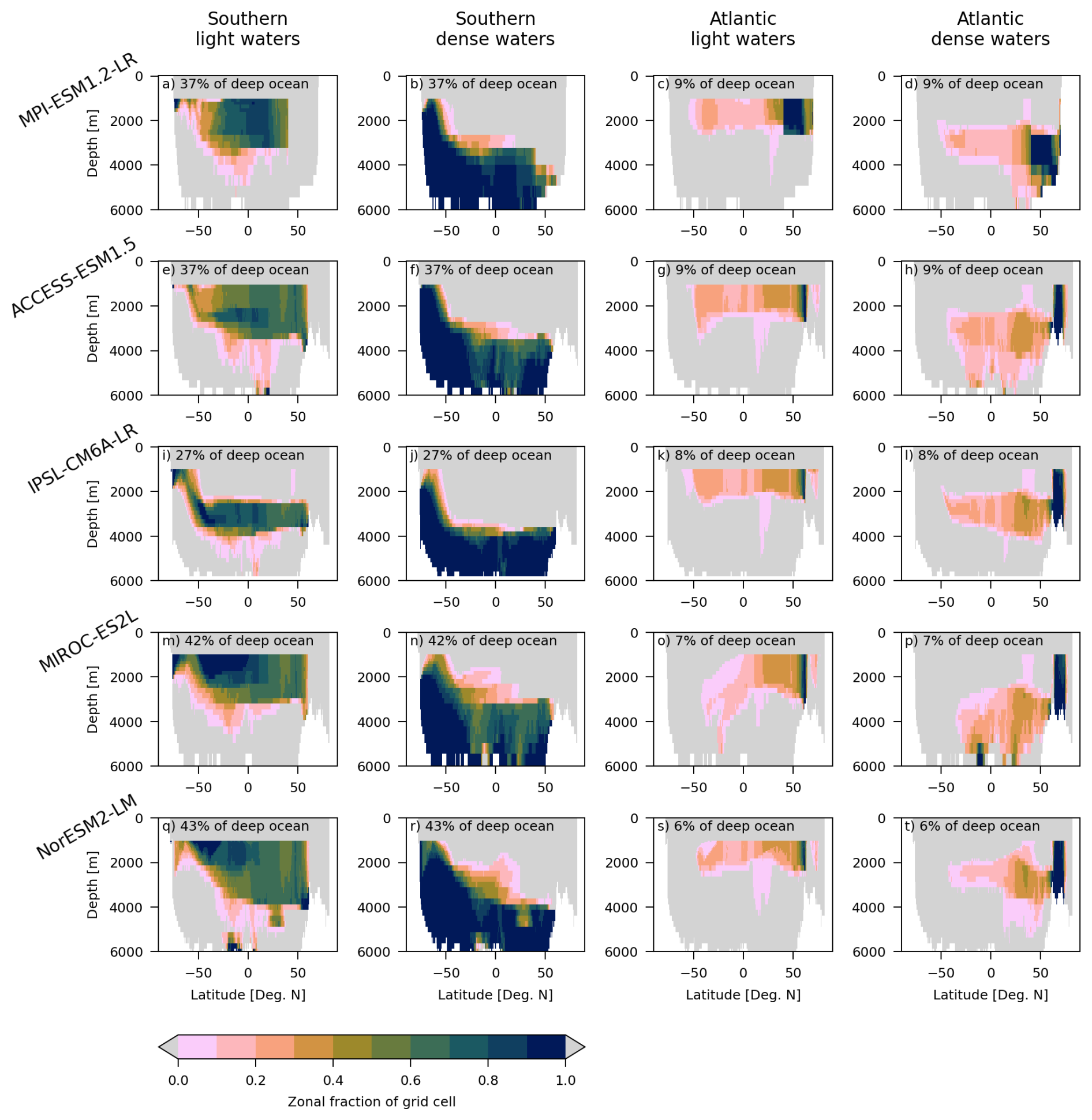
Figure A3 Similar to Fig. A2 but with the water-masses defined using PO-tracer and density fields averaged over the 2050–2099 period: distribution of the four water-masses – Southern light, Southern dense, Atlantic light, Atlantic dense, from left to right – in the five ESMs: MPI-ESM1.2-LR, ACCESS-ESM1.5, IPSL-CM6A-LR, MIROC-ES2L, NorESM2-LM, arranged from top to bottom. Each depth-latitude sections represent the zonal fraction of grid-cell belonging to the water-mass. For instance, one indicates that all the grid cells zonally belong to the water-mass, while 0.5 indicates that half of the grid cells zonally belong to the water-mass. Areas in grey depict regions where no grid cells are assigned to the water-mass. Percentages indicate the fraction of the deep ocean volume covered by each water-mass.

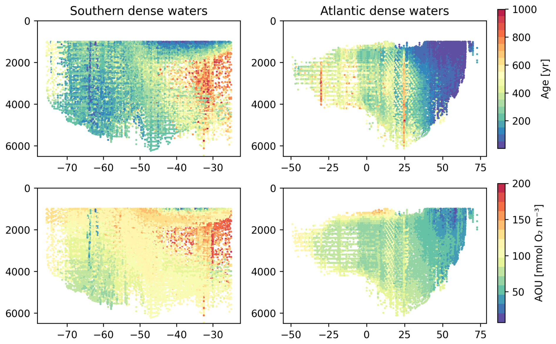
Figure A4 Latitude-depth sections of TTD-mean-age (top panels) and AOU (bottom panels) in the Southern dense (left panels) and Atlantic dense (right panels) water-masses from the observation dataset. Each dot represent one data point.

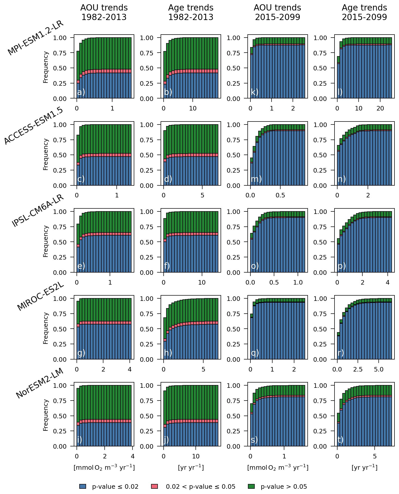
Figure A5 Cumulative histogram of trends in AOU and trends in ventilation age for the time periods 1982–2013 and 2015–2099, organized in rows, across five ESMs: MPI-ESM1.2-LR, ACCESS-ESM1.5, IPSL-CM6A-LR, MIROC-ES2L, and NorESM2-LM, listed from top to bottom. The trends are calculated using a linear regression. Each bin shows the frequency of trends, divided into three groups based on p-values: blue represents trends with p-values below 0.02 for both AOU and age; pink represents trends with p-values below 0.05 for both AOU and ventilation age but at least one of the two is above 0.02; and green represents trends with p-values above 0.05 for both. We only consider grid-points in the ocean deeper that 1000 m.

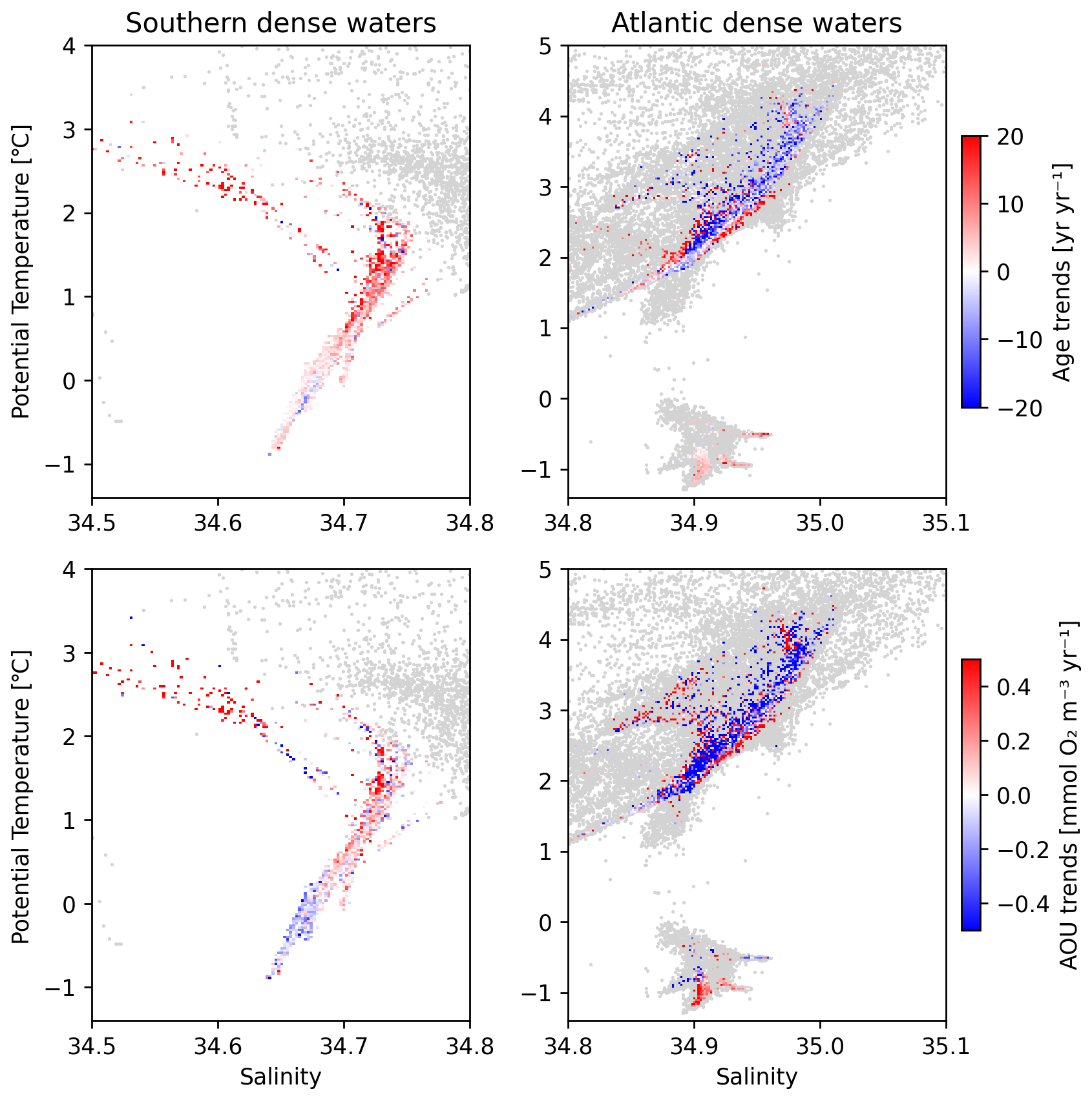
Figure A6 Trends in TTD-mean-age (top panels) and trends in AOU (bottom panels) over the 1982–2013 period from the observational dataset represented in T-S-space. Left panels show the trends in the Southern dense water-mass while the right panels the trends in the Atlantic dense water-mass. Grey shading show the rest of the data not belonging to any of the two water-masses. Here the T-S-space is divided into 350×300 T-S-bins, i.e. a resolution of 0.027 °C and 0.0023 for temperature and salinity, respectively.

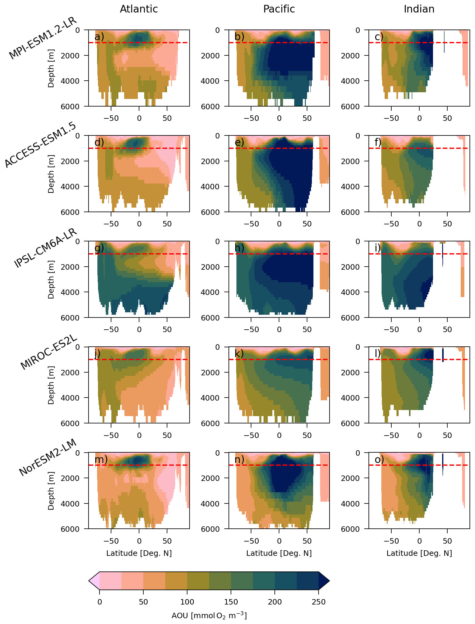
Figure A7 Contemporary (1971–2000) depth-latitude sections of AOU in five ESMs: MPI-ESM1.2-LR, ACCESS-ESM1.5, IPSL-CM6A-LR, MIROC-ES2L, and NorESM2-LM – listed from top to bottom. AOU values are zonally averaged across three ocean sectors: the Atlantic (10 to 60° W), the Pacific (130 to 180° W) and the Indian (40 to 90° E), organized from left to right. The red dashed lines indicate the 1000 m depth, separating the upper ocean from the deep ocean.

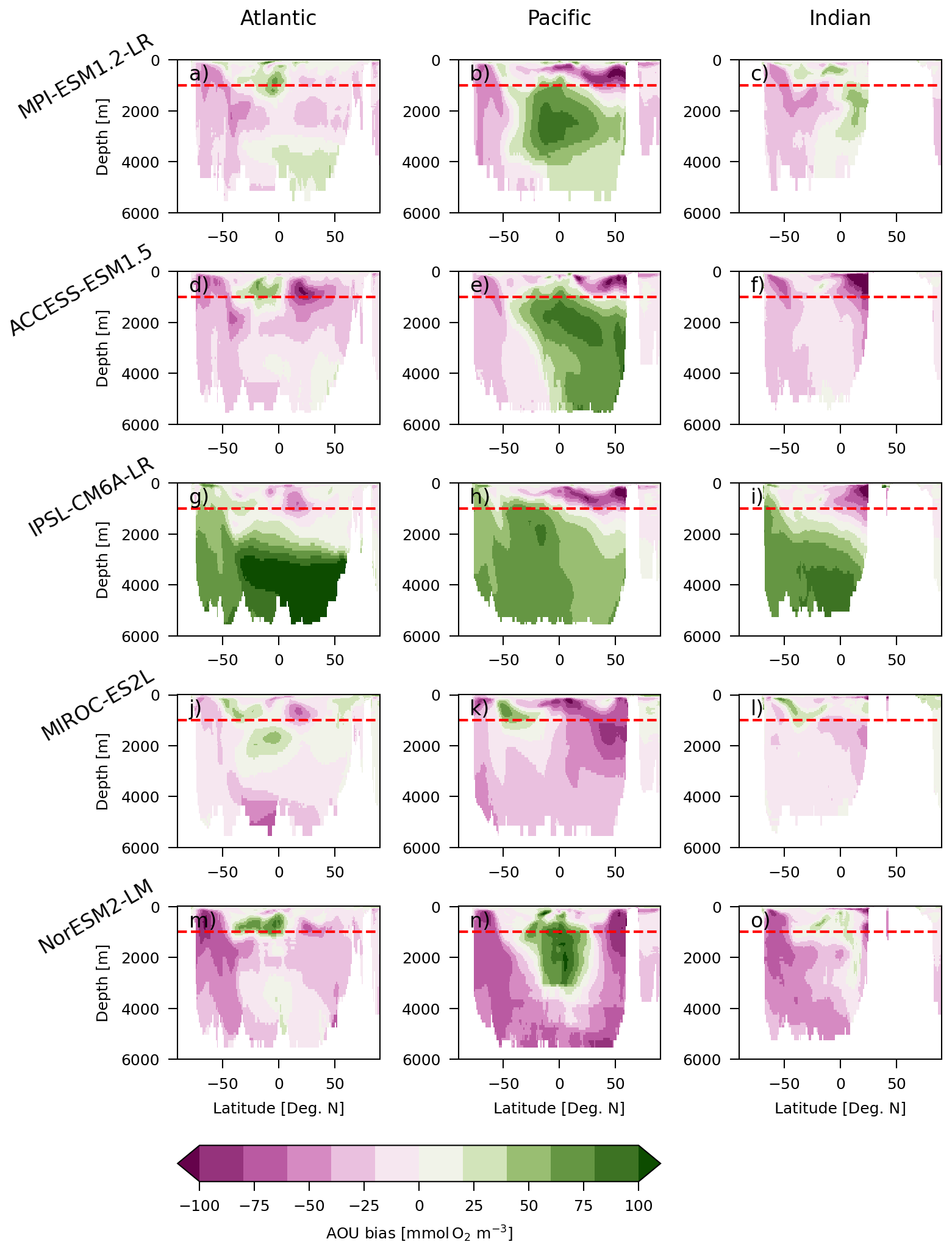
Figure A8 Contemporary (1971–2000) depth-latitude sections of AOU bias against World Ocean Atlas 2023 (WOA23, Garcia et al., 2024) in five ESMs: MPI-ESM1.2-LR, ACCESS-ESM1.5, IPSL-CM6A-LR, MIROC-ES2L, and NorESM2-LM – listed from top to bottom. AOU bias are zonally averaged across three ocean sectors: the Atlantic (10 to 60° W), the Pacific (130 to 180° W) and the Indian (40 to 90° E), organized from left to right. The red dashed lines indicate the 1000 m depth, separating the upper ocean from the deep ocean.

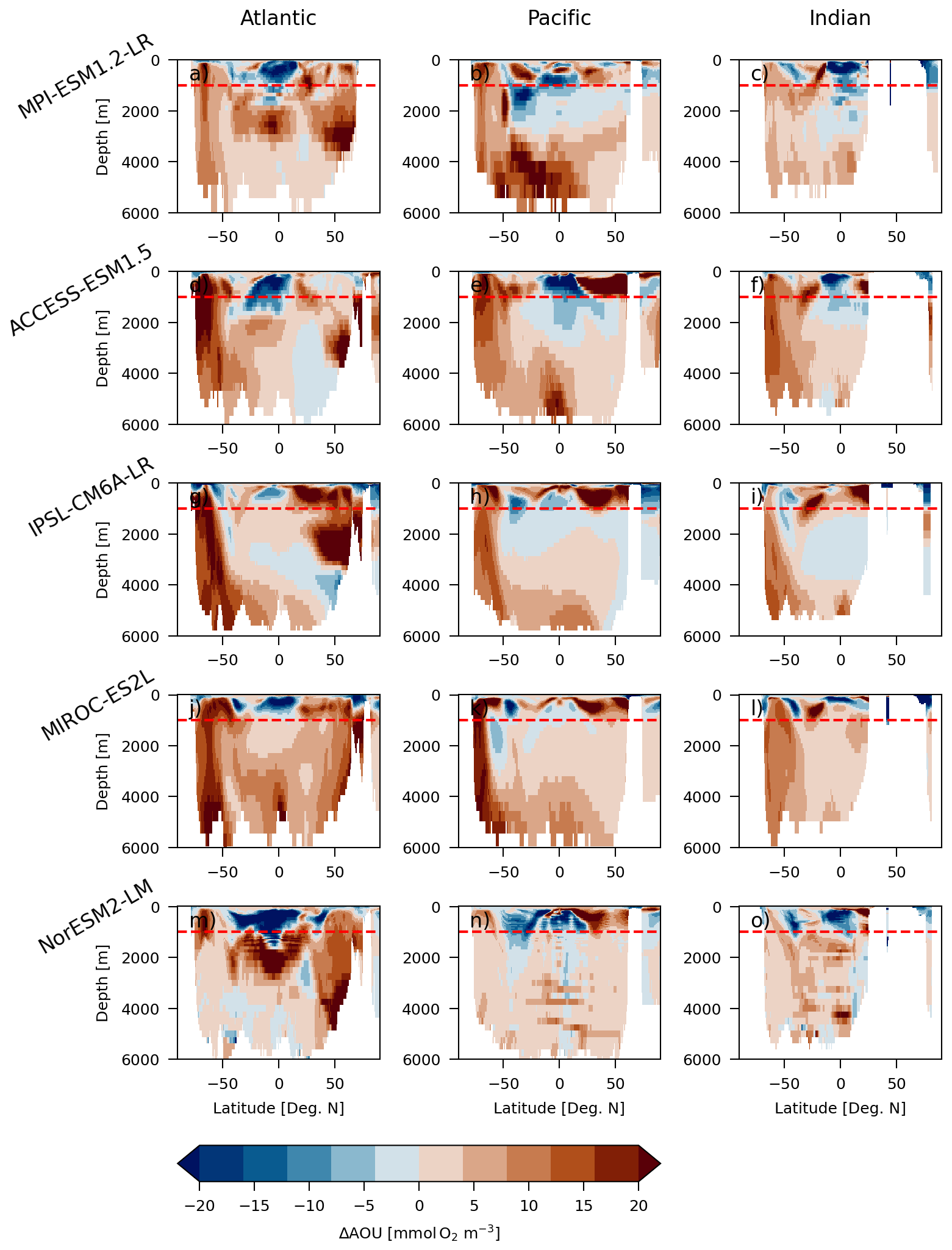
Figure A9 Depth-latitude sections of projected change in AOU (ΔAOU) under the SSP5-8.5 scenario in five ESMs: MPI-ESM1.2-LR, ACCESS-ESM1.5, IPSL-CM6A-LR, MIROC-ES2L, and NorESM2-LM – listed from top to bottom. ΔAOU is computed as the difference between years 2070–2099 and 1971–2000 and then is zonally averaged across three ocean sectors: the Atlantic (10 to 60° W), the Pacific (130 to 180° W) and the Indian (40 to 90° E), organized from left to right. The red dashed lines indicate the 1000 m depth, separating the upper ocean from the deep ocean.

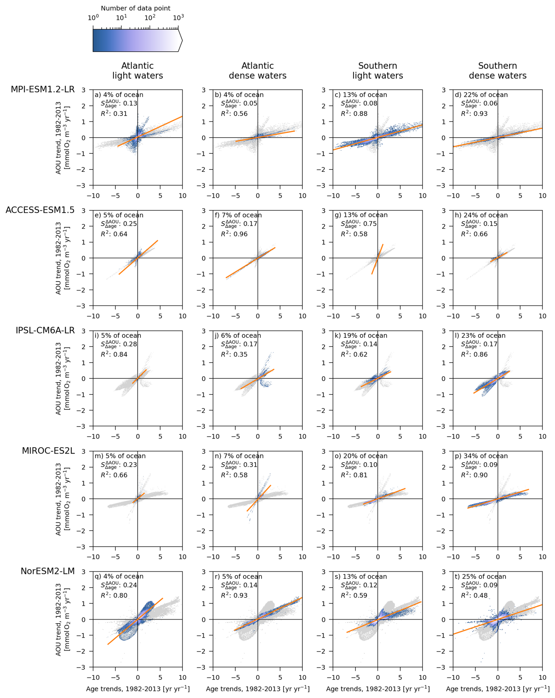
Figure A10 Distribution of the trends in ideal-age and AOU in each individual water-mass. The trends are computed on years 1982 to 2013 after removing the model drift. The non-significant trends (p-value>0.05) have been excluded. The blue shading shows the number of data point for each bins of ideal-age trends and AOU trends. The gray shading show the distribution of trends for the entire ocean. A linear regression is computed between the AOU trends and ideal-age trends for each water-mass. On each panel are shown the slope ($S_{\mathrm{\Delta }\text{age}}^{\mathrm{\Delta }\text{AOU}}$), the coefficient of determination (R²) and the fraction of the deep ocean volume.

Figure A11 Similar to Fig. 2 in the main manuscript but for the future period (2015–2099): distribution of the trends in ideal-age and trends in AOU simulated with five ESMs: (a) MPI-ESM1.2-LR, (b) ACCESS-ESM1.5, (c) IPSL-CM6A-LR, (d) MIROC-ES2L, (e) NorESM2-LM. For each ESM the x axis shows the trends in ideal-age and the y axis the trends in AOU. The trends are computed on years 2015 to 2099 after removing the model drift. The non-significant trends (p-value>0.05) have been excluded. The blue shading shows the number of data point for each bins of ideal-age trends and AOU trends for the Southern and Atlantic light/dense waters. These waters cover the majority of the deep ocean (>1000 m), see methods for their definition. A linear regression is computed between the AOU trends and ideal-age trends for each water-mass. On each panel, the slope ($S_{\mathrm{\Delta }\text{age}}^{\mathrm{\Delta }\text{AOU}}$), the coefficient of determination (R²) and the fraction of the deep ocean volume are shown in different colours for the four different water-masses. The gray shading show the distribution of trends for the entire ocean.

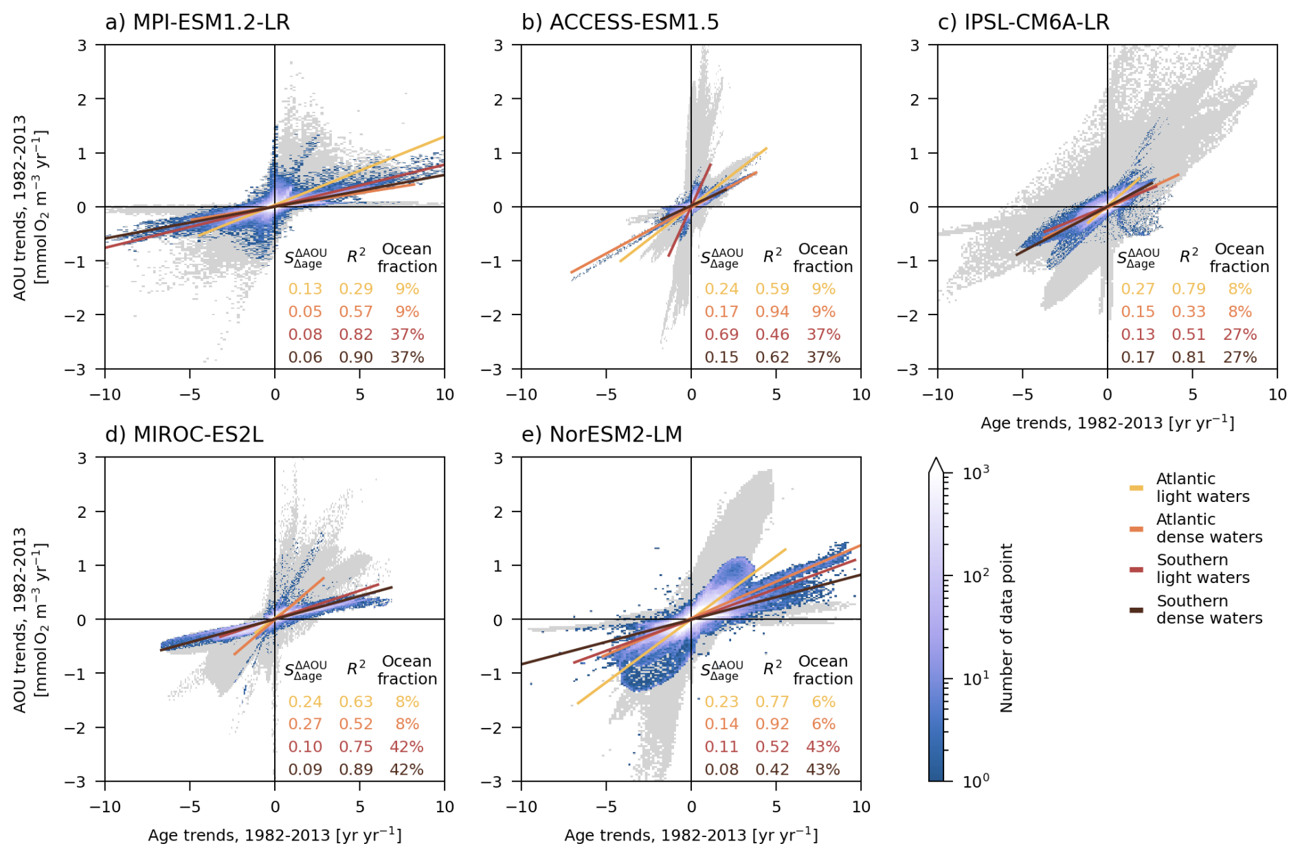
Figure A12 Similar to Fig. 2 in the main manuscript but including trends with low significance (p-value>0.05): distribution of the trends in ideal-age and trends in AOU for the contemporary period (1982–2013) simulated with five ESMs: (a) MPI-ESM1.2-LR, (b) ACCESS-ESM1.5, (c) IPSL-CM6A-LR, (d) MIROC-ES2L, (e) NorESM2-LM. For each ESM the x axis shows the trends in ideal-age and the y axis the trends in AOU. The trends are computed on years 1982 to 2013 after removing the model drift. The blue shading shows the number of data point for each bin of ideal-age trends and AOU trends for the Southern and Atlantic light/dense waters. These waters cover the majority of the deep ocean (>1000 m), see methods for their definition. A linear regression is computed between the AOU trends and ideal-age trends for each water-mass. On each panel, the slope ($S_{\mathrm{\Delta }\text{age}}^{\mathrm{\Delta }\text{AOU}}$), the coefficient of determination (R²) and the fraction of the deep ocean volume are shown in different colours for the four different water-masses. The gray shading show the distribution of trends for the entire ocean.

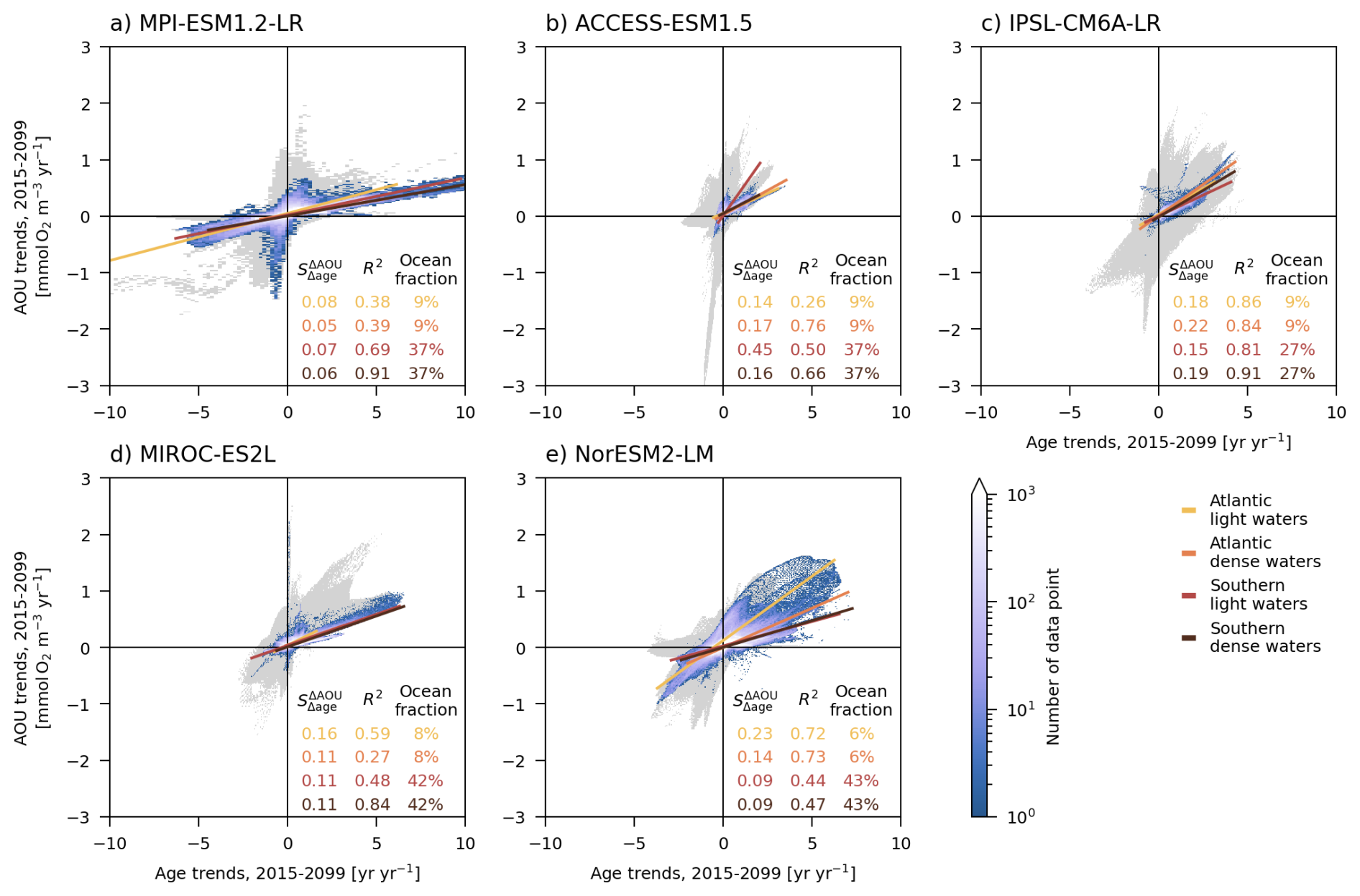
Figure A13 Similar to Fig. A11 but including trends with low significance (p-value>0.05): distribution of the trends in ideal-age and trends in AOU for the future period (2015–2099) simulated with five ESMs: (a) MPI-ESM1.2-LR, (b) ACCESS-ESM1.5, (c) IPSL-CM6A-LR, (d) MIROC-ES2L, (e) NorESM2-LM. For each ESM the x axis shows the trends in ideal-age and the y axis the trends in AOU. The trends are computed on years 2015 to 2099 after removing the model drift. The blue shading shows the number of data point for each bin of ideal-age trends and AOU trends for the Southern and Atlantic light/dense waters. These waters cover the majority of the deep ocean (>1000 m), see methods for their definition. A linear regression is computed between the AOU trends and ideal-age trends for each water-mass. On each panel, the slope ($S_{\mathrm{\Delta }\text{age}}^{\mathrm{\Delta }\text{AOU}}$), the coefficient of determination (R²) and the fraction of the deep ocean volume are shown in different colours for the four different water-masses. The gray shading show the distribution of trends for the entire ocean.

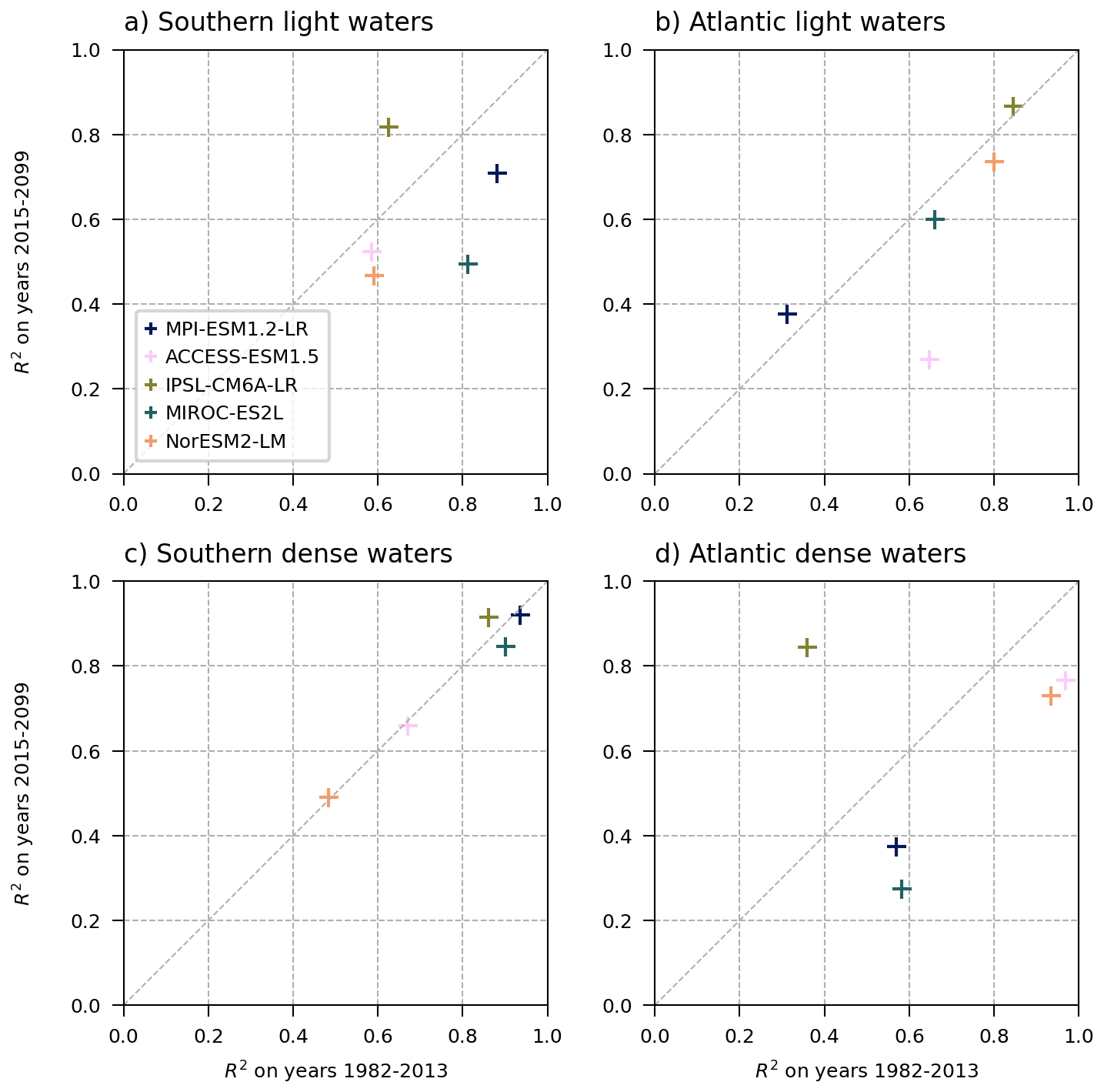
Figure A14 Distribution of the coefficient of determination (R²) from the linear regression between AOU trends and ideal-age trends in each water-masses: (a) Southern light, (b) Atlantic light, (c) Southern dense, (d) Atlantic dense. Each cross shows R² for one ESM on the contemporary (1982–2013) and future (2015–2099) period. The diagonal dashed gray line is the 1:1 line.

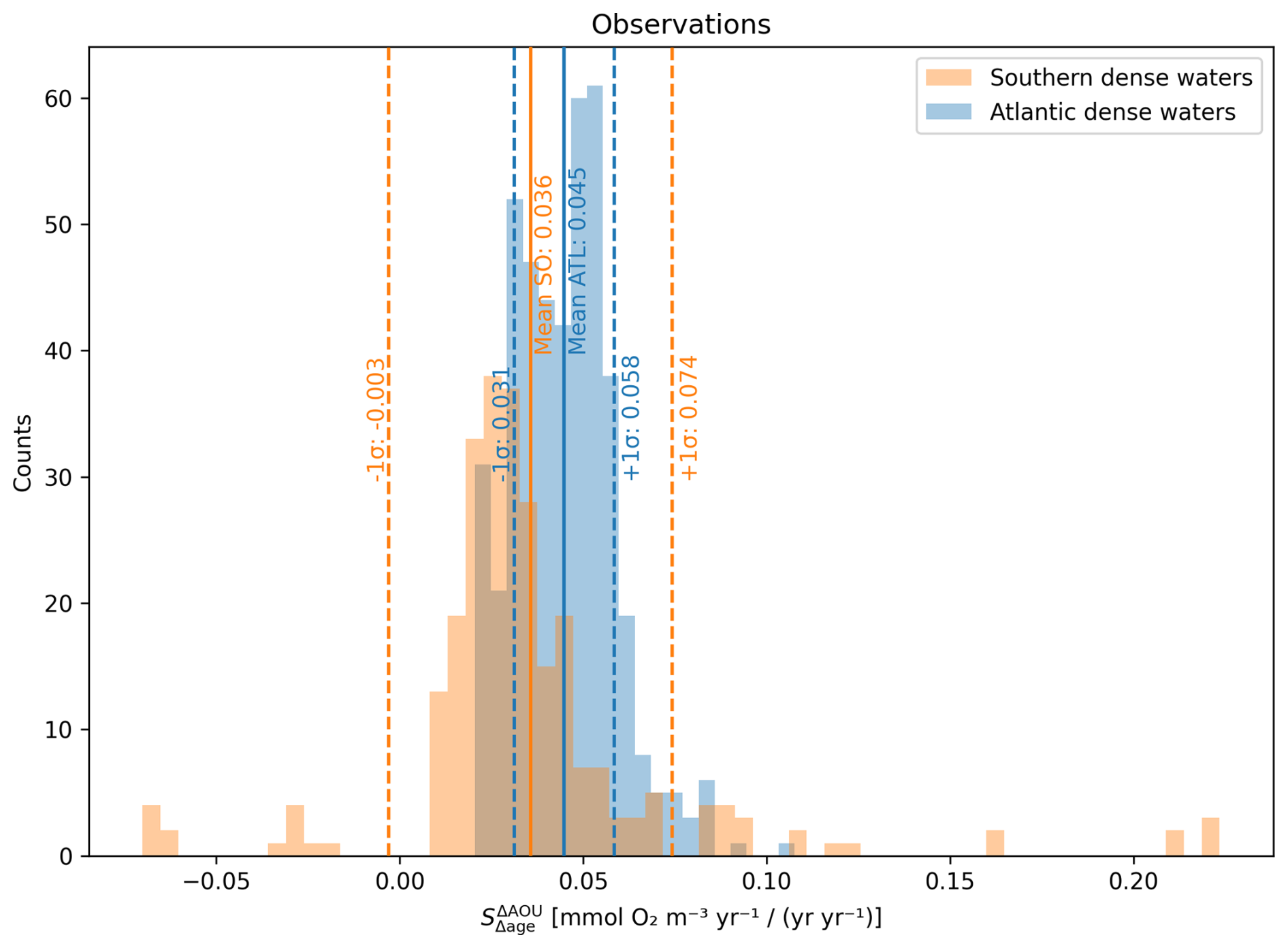
Figure A15 Distribution of $S_{\mathrm{\Delta }\text{age}}^{\mathrm{\Delta }\text{AOU}}$ estimations from the observational dataset in Southern dense (orange shading) and Atlantic dense (blue shading) water-masses for the contemporary period (1982–2013). Shown are 2500 estimations with random choices of the T-S-bins size and the geographical constraint (see methods section). Vertical lines indicate the mean (solid line) and mean plus/minus one standard deviation (dashed lines).

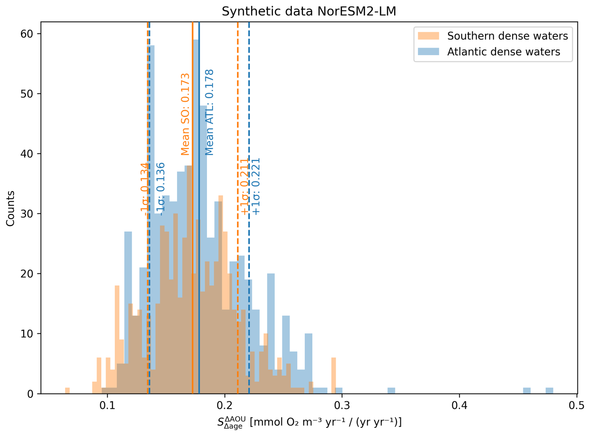
Figure A16 Similar to Fig. A15 but using a sample from NorESM2-LM outputs. The sampling mirrors the spatio-temporal distribution of the observational data. Ideal-age replaces TTD-mean-age. As in the observational dataset analysis, $S_{\mathrm{\Delta }\text{age}}^{\mathrm{\Delta }\text{AOU}}$ is estimated 2500 times with random choices of the T-S-bins size and the geographical constraint (see methods section). Vertical lines indicate the mean (solid line) and mean plus/minus one standard deviation (dashed lines).