The North Balearic Front as an ecological boundary: zooplankton fine-scale distribution patterns in late spring

Observations, models and theory have suggested that ocean fronts are ecological hotspots, generally associated with higher diversity and biomass across many trophic levels. Nutrient injections are often associated with higher chlorophyll concentrations at fronts, but the response of the zooplankton community is still insufficiently understood. The present study investigates mesozooplankton

stocks and composition during late spring, northeast of Menorca, along two north-south transects that crossed the North Balearic Front separating central waters of the Northwestern Mediterranean Sea gyre from peripheral waters originating from the Algerian basin. During the BioSWOT-Med campaign, vertical triple-net tows with 200 and 500 µm meshes were carried out at three depths (100, 200, and 400 m), and the samples were processed with ZooScan to classify organisms into eight taxonomic groups. Zooplankton distributions were analyzed for the surface layer (0–100 m), a mid-depth layer (100–200 m), and a deeper

layer (200–400 m). The results did not show a significant increase in biomass in the front in any layers. The NBF appears to act as a boundary between communities rather than a pronounced area of active or passive zooplankton accumulation. Analyses of stratified vertical distributions of zooplankton highlighted distinct taxonomic compositions in the three layers, and a progressive homogenization of community structure with depth, reflecting a weaker impact of hydrological processes on deeper communities. The clearest impact of the front was within the upper 100 m, where the mesozooplanktonic taxonomic composition differed

between the front and adjacent water masses, with a decrease in all taxonomic groups except Cnidaria, which increased dramatically. In the two deeper layers, the front also influenced community composition, although to a lesser extent, with marked increases in Foraminifera and Cnidaria. Moreover, the northern water mass and the front were dominated by large copepods, while the southern water mass exhibited higher zooplankton diversity and smaller-sized copepods. The results of this study highlight the complexity of processes shaping planktonic communities over time and space in the NBF zone and its adjacent waters. These processes include

zooplankton stock reduction in the transitional post-bloom period, marked effect of diel variation linked to vertical migrations, and potentially the impact of storm-related mixing in the surface layer that can disrupt established ecological patterns.

1 Introduction

Oceanic fronts are narrow regions of elevated physical gradients that separate water parcels with distinct properties, such as temperature, salinity, and consequently density (Hoskins, 1982; Joyce, 1983; Pollard and Regier, 1992; Belkin and Helber, 2015).

These frontal zones act as dynamic boundaries between distinct water masses (Ohman et al., 2012; Mańko et al., 2022), which play a crucial role in shaping marine ecosystems (Belkin et al., 2009). Moreover, fronts display wide variations in spatial and temporal dimensions ranging from hundreds of meters to tens of kilometers, and from short-lived to permanent (Owen, 1981; McWilliams, 2016; Lévy et al., 2018). Fronts are key structural features of the ocean, affecting all trophic levels across a wide range of spatial and temporal scales (Belkin et al., 2009).

The relationships between fronts and plankton have received considerable attention in marine ecology due to the enhanced biological production and community changes that are sometimes observed in their vicinity (Le Fèvre, 1987; Fernández et al., 1993; Pinca and Dallot, 1995; Errhif et al., 1997; Pakhomov and Froneman, 2000; Chiba et al., 2001; Munk et al., 2003). As physical barriers or zones of mixing, fronts structure biomass and species distributions, generally leading to distinct ecological communities on either side (Ohman et al., 2012; Le Fèvre, 1987; Prieur and Sournia, 1994; Gastauer and Ohman, 2024). They are often associated with enhanced nutrient input through cross-frontal mixing and vertical circulation (Durski and Allen, 2005; Liu et al., 2003; Derisio et al., 2014; Russell et al., 1999), which stimulates phytoplankton production, sustains zooplankton stocks and metabolism activity (Thibault et al., 1994; Ashjian et al., 2001; Ohman et al., 2012; Derisio et al., 2014; Powell and Ohman, 2015a), and supports higher trophic levels such as fish larvae, tuna, seabirds, and whales (Herron et al., 1989; Olson et al., 1994; Royer et al., 2004; Queiroz et al., 2012; Di Sciara et al., 2016; Druon et al., 2019). Pronounced changes in zooplankton diel vertical migration (DVM) have also been observed across frontal gradients (Powell and Ohman, 2015b; Gastauer and Ohman, 2024).

Recent studies (Mangolte et al., 2023; Panaïotis et al., 2024) have highlighted the importance of investigating zooplankton distribution at fine scales and their patchiness in the vicinity of fronts to understand their interactions with particles (e.g., organic detritus and prey items) and the environment. Mangolte et al. (2023) revealed that the plankton community exhibits fine-scale variability across fronts, with biomass peaks of different taxa often occurring on opposite sides of the front, or with different spatial extents. This fine-scale cross-frontal patchiness suggests processes leading to the spatial decoupling of plankton taxa, and to the formation of multiple adjacent communities rather than a single coherent frontal plankton community.

In the Northwestern Mediterranean Sea (NWMS), the role of mesoscale structures in the open ocean, such as density fronts and eddies, on the distribution and diversity of zooplankton has been widely documented (Saiz et al., 2014). These structures generally increase the patchiness and activity of plankton, and stimulate trophic transfers to large predators (Cotté et al., 2009, 2011). However, among the most pronounced geostrophic frontal zones in the NWMS, the North Balearic Front (NBF) and its ecological impacts remain among the least studied. In this context, the BioSWOT-Med cruise offered a unique opportunity to investigate how mesoscale oceanographic features influence zooplankton communities across the NBF, which separates the water masses of the Provencal Basin to the north and the Algerian Basin to the south.

This interdisciplinary campaign combined satellite observations with a wide range of in situ measurements, including current profiling, vertical velocity, moving vessel profilers, gliders, drifters, floats, biogeochemical analyses, genomics, phytoplankton and zooplankton sampling. Zooplankton communities were sampled using various net tows, providing insights into their composition and spatial variability across frontal gradients.

In this study, we hypothesize that zooplankton communities differ between the water masses on either side of the front, reflecting both the front's barrier effect and the distinct origins of the two water masses. From this assumption, several questions arise: how are zooplankton communities structured on each side of the front; does the frontal zone host a mixture from both water masses, or whether it sustains its own assemblage; does the front affect the vertical distribution of zooplankton communities; and to what extent weather events, such as storms, influence the structure of zooplankton communities?

2 Materials and methods

2.1 Study area

The study was conducted in the NWMS (Fig. 1) as part of the BioSWOT-Med cruise (https://doi.org/10.13155/100060; PIs: A. Doglioli and G. Grégori) and specifically in the frontal zone associated with the Balearic current. Due to its coastal proximity, the frontal zone of the Northern Current (NC) (Fig. 1) has been widely studied from physical and ecosystem perspectives, on both the Ligurian side (Prieur et al., 1983; Stemmann et al., 2008) and the Catalan side (Font et al., 1988; Sabatés et al., 2007). Downstream of the NC, the North Balearic current flows from northeast Menorca to southwest Corsica. This current is associated with the

NBF, which marks the transition between two contrasting surface water masses: the saltier, colder, and more productive waters from the Provençal Basin to the north (hereafter called water mass A), and the fresher, warmer, and less productive waters from the Algerian Basin to the south (hereafter called water mass B). The sharp frontal region separating them is designated as F (Fig. 2). Recent contributions from glider data and satellite imagery have allowed us to better characterize the NBF (Barral, 2022). Its latitudinal position varies seasonally (from 40.2° N in spring to 41° N in autumn) and also inter-annually. These shifts are linked to

the intensity and extent of winter deep convection in the northern Provençal Basin, and to mesoscale dynamics to the south, where lighter Atlantic waters are advected north between Menorca and Sardinia (Millot, 1999; Seyfried et al., 2019). The BioSWOT-Med cruise was carried out on board the R/V L'Atalante (FOF-French Oceanographic Fleet) from 21 April to 14 May 2023 in an area about 100 km north-east of Menorca Island (NWMS) (Fig. 2). Figure 2a shows the zone as observed four days before the first transect, due to cloud cover during the first days of the survey (Fig. A1).

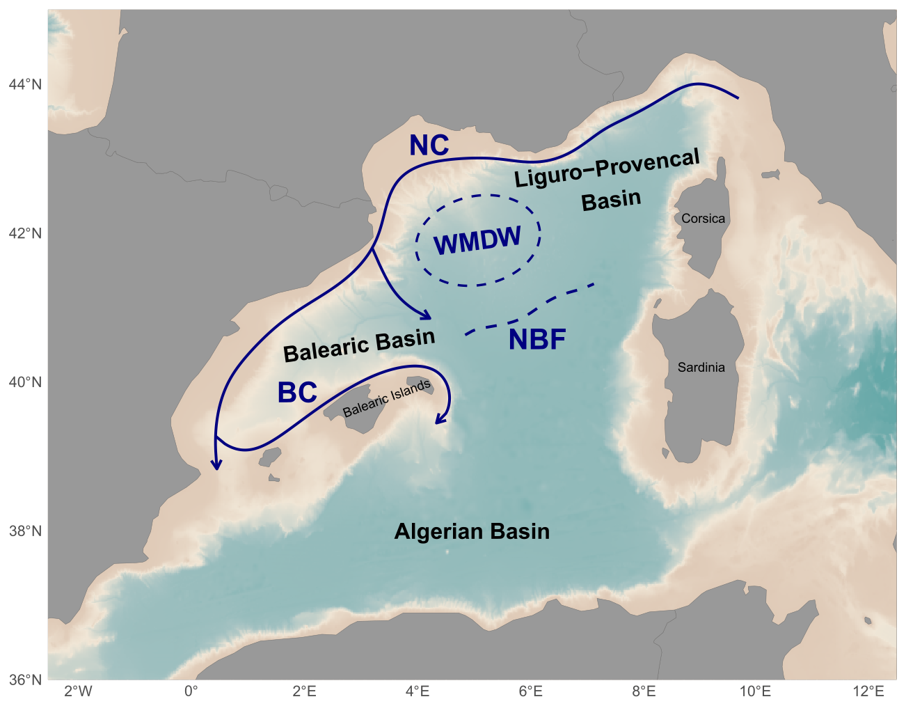
Figure 1 Maps of the NWMS showing the major oceanographic currents and front (NC: Northern Current, BC: Balearic Current, NBF: North Balearic Front, WMDW: Western Mediterranean Deep Water formation area) of the northern part of the NWMS. After Millot (1987), López García et al. (1994), Pinardi and Masetti (2000).

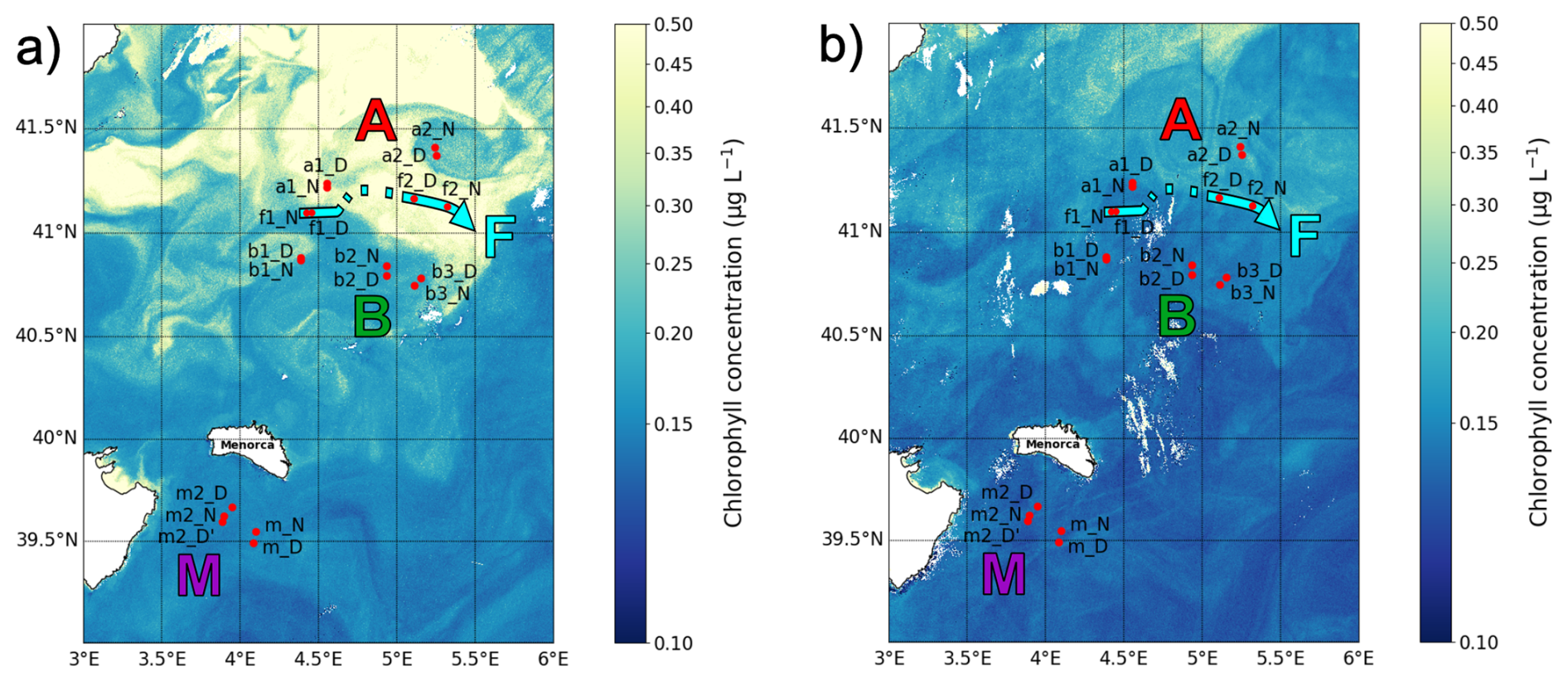
Figure 2 Maps of the sampling stations with surface chlorophyll concentration (µg L⁻¹) from Sentinel-3. (a) Map from 21 April showing conditions 4 d before the first transect. (b) Map from 5 May showing conditions during the second transect. The colors representing the three water masses and the front will be maintained throughout the paper.

2.2 Sampling strategy

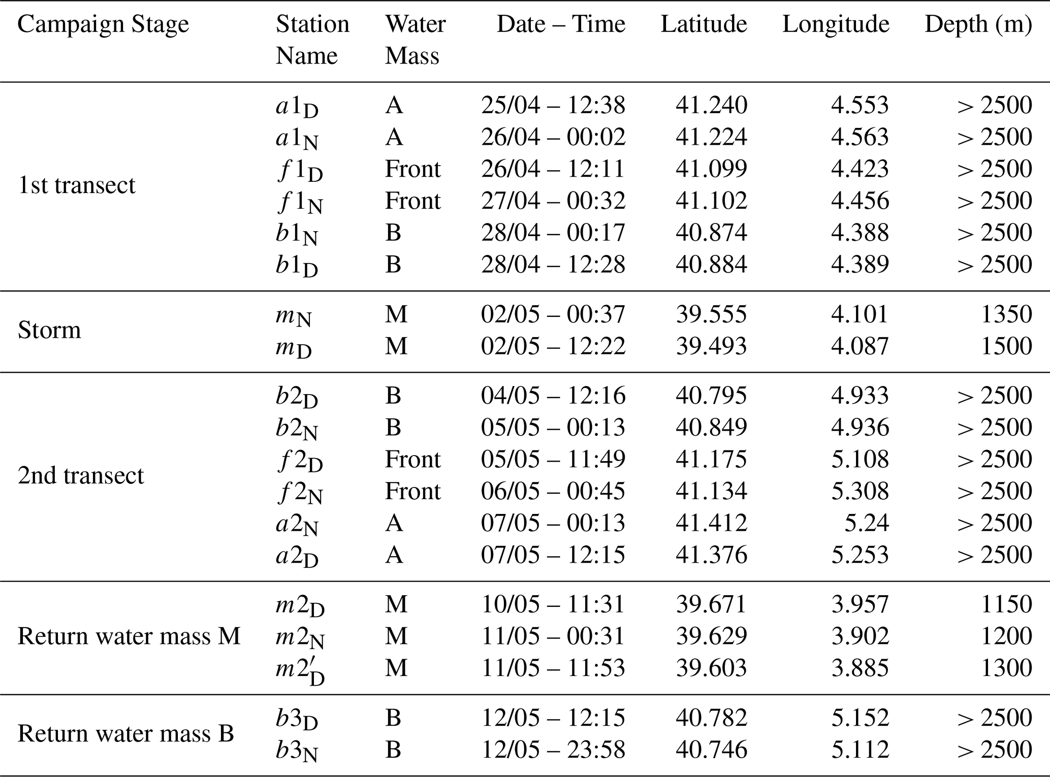
The strategy of the cruise was designed to take advantage of the novel SWOT (Surface Water and Ocean Topography) satellite mission, to resolve fine-scale oceanic features more effectively. During the “fast sampling phase”, SWOT provided altimetry data characterized by high spatial resolution (2 km) and a 1 d revisit period over 150 km-wide oceanic regions. With the support of the international SWOT AdAC (Adopt-A-Crossover, https://www.swot-adac.org/, last access: 8 January 2026; PI Francesco d'Ovidio) Consortium, the BioSWOT cruise

applied an adaptive multidisciplinary approach by combining daily SWOT images and environmental bulletins provided by the SPASSO toolbox (https://spasso.mio.osupytheas.fr/, last access: 15 October 2025, Rousselet et al., 2025). Along with in situ measurements taken using a suite of instruments to capture physical, chemical and biological properties (Doglioli et al., 2024, cruise report). This strategy enabled the targeting of fine-scale features (e.g., kilometers) of the NBF. The three main water masses (A, B, F) were each sampled at two stations: a1–a2, b1–b2, and f1–f2; with a1, b1, f1 on the first transect (westbound) and a2, b2, f2 on the second transect (eastbound).

Each station was sampled twice: at noon and midnight. Additionally, three supplementary stations (b3, m, and m2) were sampled (Table 1, Fig. 2). At each station, the vessel remained within the same water mass for 24 h, drifting slightly with the currents during the sampling period, which explains the small differences in station location between day and night (Fig. 2). The two f2 stations were relatively distant from each other due to a strong frontal current. Because of a storm on 2 May, a third area, “M”, was sampled twice while the ship took shelter south of Menorca, where similar measurements were conducted as in zones A, B, and F.

The M zone differs from the three other sampled zones in terms of bathymetry (Table 1), as it was located around 20 km from the continental shelf. On the way home, a final station was sampled in B (Table 1). At every station, physical properties were recorded using a CTD rosette, which was deployed four times daily at fixed intervals (06:00, 12:00, 18:00, and 00:00 local time). Hereafter, water masses will be designated by an uppercase letter (A, B, M, and F for the front), and stations by a lowercase letter (a, b, m, f).

Table 1 Station details. In Station Name, “D” stands for day and “N” stands for night. Depth values are approximate (± 50 m) for the station within the water mass M. Depths indicated as “> 2500” correspond to stations deeper than 2500 m.

2.3 Zooplankton collection

Zooplankton samples were collected using a triple net (Triple-WP2) equipped with three individual nets, each with a 60 cm mouth diameter, but different mesh sizes (64, 200 and 500 µm). For this study, which focuses on mesozooplankton, only the samples collected by 200 and 500 µm nets were used. The nets were deployed vertically to cover three integrated layers (400–0, 200–0, 100–0 m). Note that the net deployed to 400 m at station m_N could not be analyzed because it was found folded up on itself upon retrieval. The filtered water volume was not measured with a flowmeter but estimated from the net mouth area and the tow distance. After collection, samples were preserved in 4 % borate-buffered formaldehyde solution.

2.4 Zooplankton sample processing

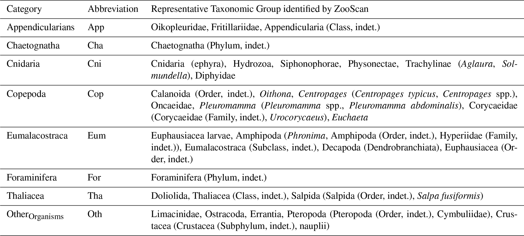
In a shore-based laboratory (Mediterranean Institute of Oceanography (MIO), Marseille, France), samples were digitized with the ZooScan digital imaging system (Gorsky et al., 2010) to identify and determine the size structure of the zooplankton communities. Each sample, from the 200 and 500 µm nets, was divided into two size fractions (< 1000 and > 1000 µm) for better representation of rare large organisms in the scanned subsample (Vandromme et al., 2012). Each fraction was split using a Motoda box (Motoda, 1959) until it contained an appropriate number of objects, approximately 1500, according to Gorsky et al. (2010). After scanning, each image was processed using ZooProcess (Gorsky et al., 2010), which runs within the ImageJ image analysis software (Rasband, 1997–2011). Only objects having an Equivalent Circular Diameter (ECD) > 300 µm were detected and processed (Gorsky et al., 2010). Objects were first automatically classified using ECOTAXA (https://ecotaxa.obs-vlfr.fr/, last access: 10 November 2025) on ZooScan images with a pixel size of 10.58 µm. As a result, certain taxa were successfully identified at the species level, whereas others could only be classified to the genus, family, or order levels. Certain taxa were either too small or could not be precisely recognized by EcoTaxa

for other reasons (e.g., sample condition, image quality during scanning) and therefore could not be assigned to a taxonomic level finer than the order. For example, 65 % of copepods were classified as Calanoida indeterminate. Consequently, although 101 taxa were detected, they have been grouped into eight main categories: Appendicularia, Chaetognatha, Copepoda, Cnidaria, Eumalacostraca, Foraminifera, Thaliacea, and Other_Organisms (Table 2). Table 2 does not list all recognized taxa within each of the eight categories, but only those that accounted for at least 1 % of the total concentration within their category. The last category, Other_Organisms, includes all remaining taxa that did not belong to any of the designated classes and were present in very low numbers in all samples. Zooplankton concentration (number of individuals m⁻³) was calculated from the number of validated vignettes in ZooScan samples, considering the scanned fraction and the sampled volume from the nets.

The 200 and 500 µm net samples were processed separately using ZooScan, and their resulting counts were subsequently combined. To avoid double counting of organisms large enough to be captured by both nets, a threshold value was established, based on the analysis of the Normalized Biomass Size Spectra (NBSS) (Sect. 2.7), considering all stations and depths (a specific value for each station would not have significantly altered the results). The threshold value (1148 µm ECD) identified the body size at which the 500 µm net samples more effectively (Fig. A2). Thus, organisms smaller than this size from the 200 µm net, and those larger from the 500 µm net, were combined into a new dataset, hereafter called the “combined net”.

Table 2 Zooplankton taxonomic categories and their representative groups (≥ 1 % of the concentration within their category) identified by ZooScan. Taxonomic categories labelled “indet.” denote taxa identified only to the given taxonomic rank when finer identification was not possible.

2.5 Definition of reconstructed depth layers: 100–200 and 200–400 m

Our nets sampled three layers: 0–100, 0–200, and 0–400 m (Sect. 2.3). In order to study the community by depth, the concentration of different taxonomic groups (Sect. 2.4) was calculated in each layer by differencing. For instance, subtracting the concentration measured at 0–100 m from that at 0–200 m provided values for the 100–200 m layer. A similar approach was used

to calculate the values for the 200–400 m layer. This approach was considered valid as the net tows were carried out successively within a relatively short interval of time, typically 45 min, although potential limitations are discussed in Sect. 4.4. It is important to note that subtractions were performed on the eight major categories and not on individual taxonomic groups (see Table 2). In rare cases (12 %), especially for Eumalacostraca (particularly in the 100–200 m layer) and Cnidaria (particularly in the 200–400 m layer), the resulting concentrations were negative and therefore set to zero.

2.6 Analysis of variance and Post-Hoc comparisons

Using R version 4.4.1 (Team, 2025), one-way analyses of variance (ANOVA) were conducted to test differences in absolute concentrations across each taxonomic category. Prior to performing the ANOVA, the normality of residuals was assessed using the Shapiro-Wilk test and the homogeneity of variances verified with Levene's test (car package, version 3.1-3; Fox and Weisberg, 2019). ANOVAs were then performed for five factors: water mass, layer, period (day or night), transect (storm effect) and copepod subgroup (DVM pattern). Copepod subgroups were selected if their total concentration exceeded 1 % of the overall copepod assemblage, which resulted in the selection of seven copepod taxa. For each ANOVA showing a significant result (p<0.05), Tukey's HSD post hoc tests were applied to identify significantly different groups. In addition, a permutational multivariate analysis of variance (PERMANOVA) was used to test differences in community composition between water masses. The analysis was performed on Hellinger-transformed relative concentrations of taxonomic groups, with significance assessed using 999 permutations.

2.7 Normalized Biomass Size Spectra (NBSS)

Organism size is a key indicator of community dynamics (Platt and Denman, 1977). NBSS (Platt and Denman, 1977) are widely used to study this property. For constructing the NBSS, zooplankton organisms were grouped into logarithmically increasing size classes. The total biovolume of each class was then divided by the width of its size class (Platt and Denman, 1977). The x-axis [log2 zooplankton biovolume (mm³ individual⁻¹)] was calculated as:

$$\begin{array}{}\text{(1)}& {\log }_{\mathrm{2}}\left[{\displaystyle \frac{\mathrm{Zooplankton}\mathrm{biovolume}\left({\mathrm{mm}}^{\mathrm{3}}{\mathrm{m}}^{-\mathrm{3}}\right)}{\mathrm{Concentration}\mathrm{of}\mathrm{each}\mathrm{class}\mathrm{size}\left(\mathrm{ind}{\mathrm{m}}^{-\mathrm{3}}\right)}}\right]\end{array}$$

The y-axis [log2 normalized biovolume (m⁻³)] was calculated as:

$$\begin{array}{}\text{(2)}& {\log }_{\mathrm{2}}\left[{\displaystyle \frac{\mathrm{Zooplankton}\mathrm{biovolume}\left({\mathrm{mm}}^{\mathrm{3}}{\mathrm{m}}^{-\mathrm{3}}\right)}{\mathrm{Interval}\mathrm{of}\mathrm{each}\mathrm{class}\mathrm{size}\left(\mathrm{\Delta }\mathrm{volume}\left({\mathrm{mm}}^{\mathrm{3}}\right)\right)}}\right]\end{array}$$

The NBSS thus represents the normalized biovolume as a function of the size of the organisms, both on a logarithmic scale. Biovolume data were estimated from ECD data provided by ZooProcess, using spherical approximation, which ensures a consistent metric for combining the two mesh sizes (200 and 500 µm). To investigate community characteristics across water masses and the front, taxonomic and size-based analyses were conducted focusing on copepods, which were the most abundantly sampled group. A size-based analysis was conducted using PCA (Sect. 2.8) on copepod size-class concentrations at the different stations, using the size classes defined for the NBSS (Fig. A2). For clarity, the 15 original size classes were grouped into five classes, each defined by its ECD. Other taxonomic groups were not included because their larger size ranges and the rarity of large individuals, including organisms such as chaetognaths or cnidarians, introduced substantial variability into the NBSS.

2.8 Principal Component Analysis (PCA)

PCA was used to evaluate the similarities between the stations based on the concentration of the different taxonomic groups. Distances between stations were measured in the PCA phase space after Hellinger transformation, which allows us to use relative concentrations rather than absolute concentrations. Using absolute concentrations would mainly discriminate between the first and second transects and would not reveal a stable gradient between water masses. Legendre and Gallagher (2001) also showed that the Hellinger transformation, prior to PCA, is often preferable to Euclidean distance for calculating distances between samples. Hellinger distance (Rao, 1995) is obtained from:

$$\begin{array}{}\text{(3)}& D\left(x_{\mathrm{1}},x_{\mathrm{2}}\right)=\sqrt{\sum _{j=\mathrm{1}}^p{\left(\sqrt{{\displaystyle \frac{y_{\mathrm{1}j}}{y_{\mathrm{1}+}}}}-\sqrt{{\displaystyle \frac{y_{\mathrm{2}j}}{y_{\mathrm{2}+}}}}\right)}^{\mathrm{2}}},\end{array}$$

where p denotes the number of categories, y_ij is the concentration of category j at station i and y_i+ is the sum of the concentrations of the ith object.

With this equation, the most abundant species contribute significantly to the sum of squares. The advantage of this approach is that it is asymmetric, meaning that shared absences (double zeros) do not increase similarity, unlike Euclidean distance, where they do (Prentice, 1980; Legendre and Legendre, 2012).

The Hellinger transformation was performed with the labdsv package (Roberts, 2023). The concentration tables were centered and scaled, and the PCA was computed using FactoMineR (Lê et al., 2008). Prior to carrying out PCAs, the Hellinger-transformed data were tested for normality using the Shapiro-Wilk test. Bartlett's test of sphericity was used to verify sufficient linear structure for PCA.

Stations M were not included in the main PCAs, as their inclusion can obscure the frontal signal. However, their positions as supplementary individuals are shown in the PCA plots provided in the Appendix.

2.8.1 Fixed PCA axis for comparison across layers

To obtain comparable results across depth layers, the PCAs were always conducted in the same way with fixed axes. First, a PCA was performed using data from the 0–400 m layer. Then the datasets from all three layers were projected onto the PCA axes from the 0–400 m layer. This approach ensured that comparisons between communities in the three different layers were valid.

2.8.2 Pseudo-F calculation

To quantify the separation of each water mass (A, B, F) in PCA space, the pseudo-F (Caliński and Harabasz, 1974) was used. Dispersion was calculated as the sum of squared Euclidean distances of individuals to their group centroid (intra-group dispersion), while inter-group dispersion was defined as the sum of squared distances between group centroids and the global centroid, weighted by group size. The pseudo-F statistic was calculated as follows:

$$\begin{array}{}\text{(4)}& \text{Pseudo-F}={\displaystyle \frac{\mathrm{Inter}-\mathrm{group}\mathrm{dispersion}/\left(k-\mathrm{1}\right)}{\mathrm{Intra}-\mathrm{group}\mathrm{dispersion}/\left(n-k\right)}},\end{array}$$

where k is the number of groups and n the total number of individuals.

A high pseudo-F value suggests a clear separation between groups, indicating that inter-group variation predominates over intra-group variation.

2.8.3 PCA with theoretical f stations

A fundamental question was whether the zooplankton community at the front represented a mixture of those from water masses A and B, or a distinct community. To address this, we created theoretical f_t stations, defined as linear combinations of communities from stations a and b, and chosen to minimize the distance to the observed f stations. The combination of a and b was defined as:

$$\begin{array}{}\text{(5)}& f\left\{t\right\}=\mathit{\alpha }\cdot a+(\mathrm{1}-\mathit{\alpha })\cdot b,\end{array}$$

where α is the proportional contribution from stations a and b.

A total of 101 iterations was performed, with α varying from 0 to 1 in increments of 0.01, generating four new theoretical stations per iteration:

$$\begin{array}{c}{\displaystyle }f\mathrm{1}\mathit{\{}t{\mathit{\}}}_{\mathrm{D}}={\mathit{\alpha }}_{\mathrm{1}}\cdot a{\mathrm{1}}_{\mathrm{D}}+(\mathrm{1}-{\mathit{\alpha }}_{\mathrm{1}})\cdot b{\mathrm{1}}_{\mathrm{D}}\\ {\displaystyle }f\mathrm{1}\mathit{\{}t{\mathit{\}}}_{\mathrm{N}}={\mathit{\alpha }}_{\mathrm{1}}\cdot a{\mathrm{1}}_{\mathrm{N}}+(\mathrm{1}-{\mathit{\alpha }}_{\mathrm{1}})\cdot b{\mathrm{1}}_{\mathrm{N}}\\ {\displaystyle }f\mathrm{2}\mathit{\{}t{\mathit{\}}}_{\mathrm{D}}={\mathit{\alpha }}_{\mathrm{2}}\cdot a{\mathrm{2}}_{\mathrm{D}}+(\mathrm{1}-{\mathit{\alpha }}_{\mathrm{2}})\cdot b{\mathrm{2}}_{\mathrm{D}}\\ {\displaystyle }f\mathrm{2}\mathit{\{}t{\mathit{\}}}_{\mathrm{N}}={\mathit{\alpha }}_{\mathrm{2}}\cdot a{\mathrm{2}}_{\mathrm{N}}+(\mathrm{1}-{\mathit{\alpha }}_{\mathrm{2}})\cdot b{\mathrm{2}}_{\mathrm{N}}\end{array}$$

These f_t stations were projected as supplementary points onto the PCA of the original a, b, and f stations, and therefore did not influence the axes or the positions of observed stations. For each iteration, the coordinates of the f_t stations in the PCA space were obtained, and their distances to the corresponding observed f stations were calculated. The total distance (sum of all f−f_t distances) was then computed for each transect. Finally, the f_t station with the minimum total distance, together with its corresponding α value, was selected. This procedure generated intermediate observations that best reflected the theoretical composition of the front as a linear combination of a and b.

3 Results

3.1 Total concentration across water masses and layers

The absolute values of concentration of zooplanktonic organisms across different depth layers and stations (Fig. 3) revealed distinct temporal and spatial patterns. In general, concentrations in stations within the same water mass decreased over time (stations are presented in chronological order in Fig. 3), with the exception of the front. Regarding the spatial differences during the two front crossings, concentration at the front was lower than in water masses A (2.9-fold lower) and B (1.4-fold lower) for the first transect. However, the second transect revealed greater homogeneity among water masses with values at the front only 1.1 times higher compared to water mass A and 1.9 times higher compared to water mass B, reflecting the potential influence of post-storm dynamics.

3.2 Taxonomic composition across nets and depth layers

The 200 µm net captured copepods more efficiently. In the 0–200 m layer, copepods constituted 45 %–95 % of the relative concentrations of taxa, whereas they comprised only 5 %–55 % in the 500 µm net (Fig. 4). The larger mesh size was particularly effective for sampling larger taxa such as Appendicularia, Thaliacea, Eumalacostraca, Foraminifera, Cnidaria, and Chaetognatha. The combined samples, which include contributions from both mesh sizes, still heavily reflect the taxa distributions observed in the 200 µm net, since concentrations of larger organisms sampled with the 500 µm net were low. This pattern was also observed in the layers 0–100 and 0–400 m. Moreover, during the second transect (after the storm), the dominance of copepods was enhanced in water masses A and F. All subsequent analyses were carried out on these combined nets.

In the 0–100 m layer, copepods dominated at nearly all stations (≥ 45 % of total concentrations; Fig. 5), except at b2_N. The 100–200 m layer showed marked heterogeneity, with 8 out of 18 stations having less than 60 % copepods. In the 200–400 m layer, copepods again dominated at most stations (15 out of 18), with two notable exceptions: at b2_N, where Eumalacostraca represented 55 % of the sampled taxa, and at b3_N, where Cnidaria represented 67 %.

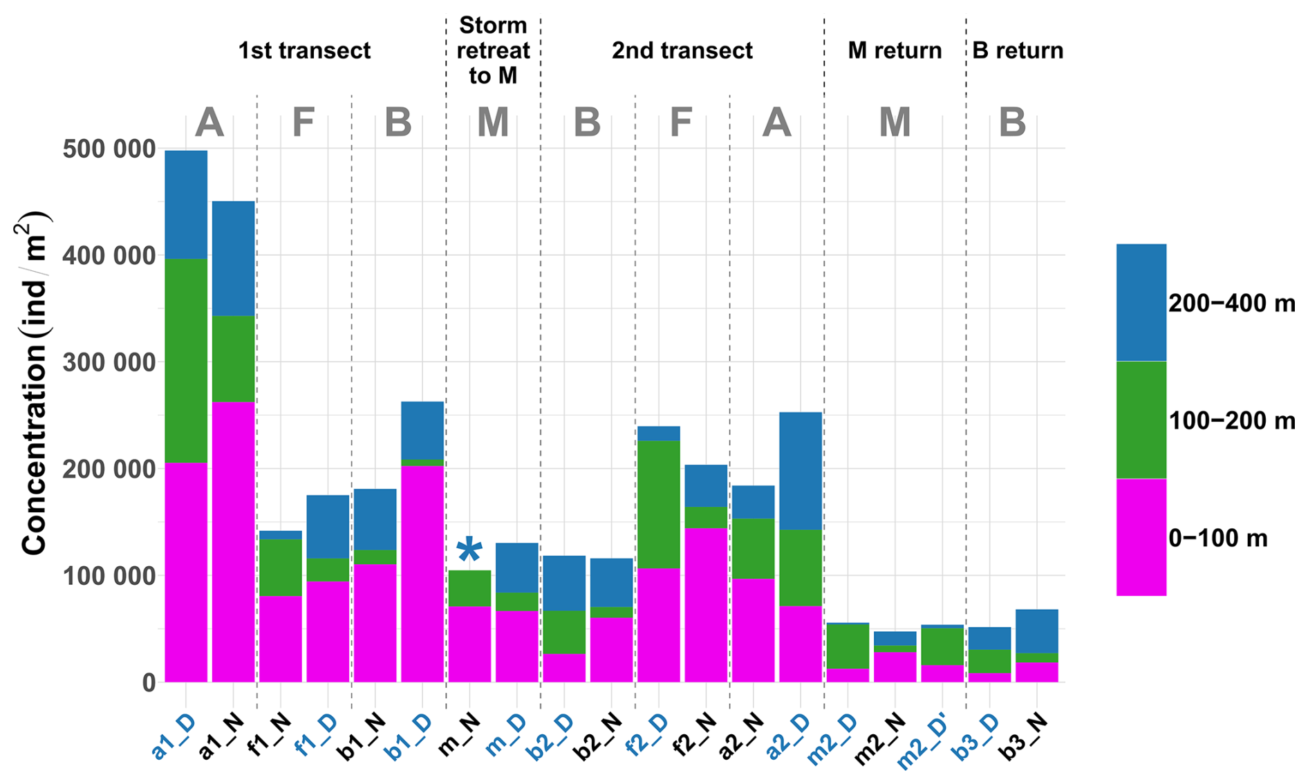
Figure 3 Stacked bar plot showing the concentration of zooplankton by reconstructed layer and across all sampled stations. Stations are in chronological order. The asterisk (^*) indicates that the 200–400 m net at station m_N could not be analyzed. Station name colors indicate the period of the day (blue: midday; black: midnight). Letters A, B, F, and M denote water masses.

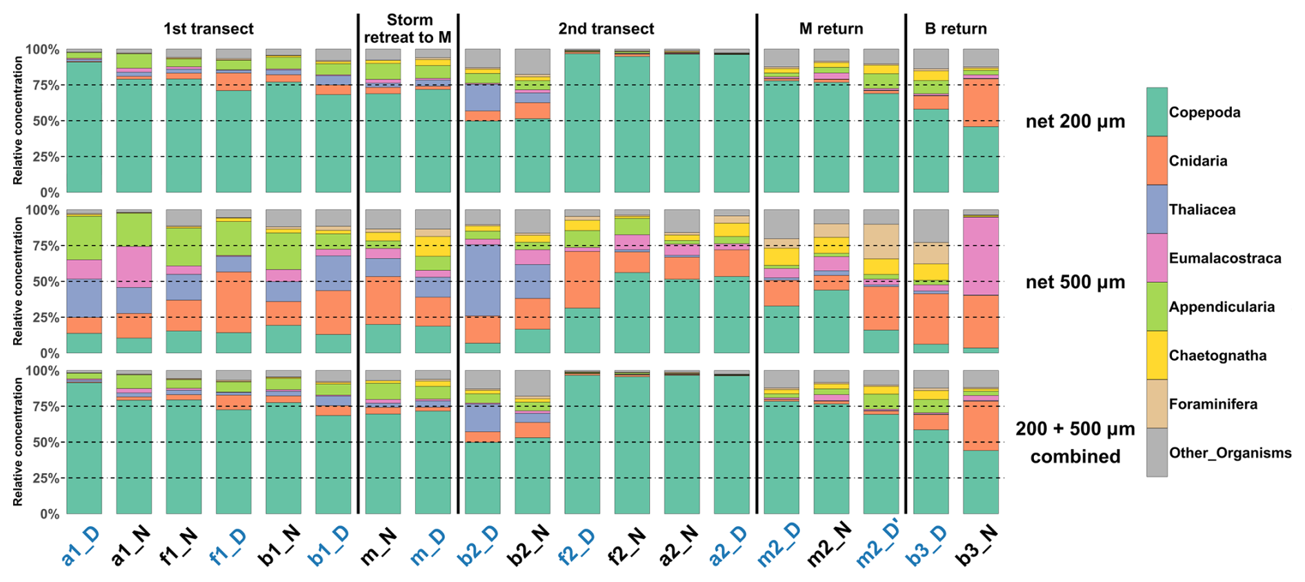
Figure 4 Relative concentration of taxonomic groups for nets deployed from the surface to a depth of 200 m, for the two mesh sizes (200 µm top, and 500 µm, middle) across all sampled stations (chronological order). Bottom: Relative concentration combining the two mesh sizes. Station name colors indicate the period of the day (blue: midday; black: midnight).

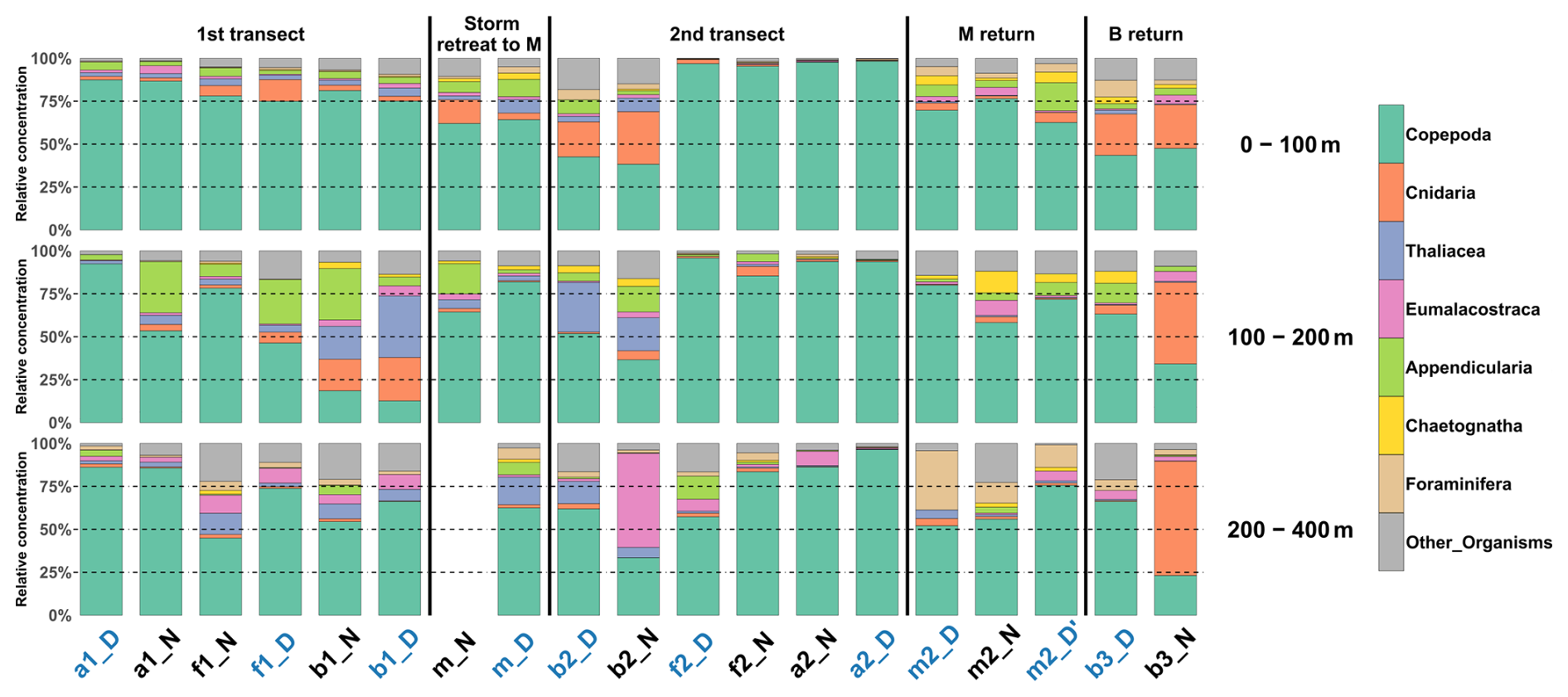
Figure 5 Relative concentration of taxonomic groups for the combined nets for the three reconstructed layers across all sampled stations (chronological order). The 200–400 m net at station m_N could not be analyzed. Station name colors indicate the period of the day (blue: midday; black: midnight).

3.3 Diel variations in vertical structuring of zooplankton stocks

Zooplankton communities seemed to show a vertical pattern, with the upper (0–100 m) and deeper (200–400 m) layers more similar to each other, and the mid-depth layer (100–200 m) more distinct (Fig. 5). Hellinger distance analysis for the eight taxonomic groups reflected this pattern: the lowest distances were observed between the 0–100 m and 200–400 m layers for Copepoda (0.04 and 0.09 for the first and second transect, respectively), Eumalacostraca (0.03 and 0.08), and Other_Organisms (0.06 and 0.03), whereas distances involving the 100–200 m layer were about 4 times higher.

A DVM pattern was evident in the two migrant groups, Copepoda and Eumalacostraca. At night, the 0–100 and 100–200 m layers were more similar, while during the day, the 100–200 and 200–400 m layers showed greater similarity. These patterns were statistically significant (post-hoc, p<0.001 and 0.008, respectively). Hellinger distances between surface (0–100 m) and deep (200–400 m) layers increased both during the day (0.24 and 0.13 for Copepoda; 0.48 and 0.38 for Eumalacostraca) and at night (0.29 and 0.34 for Copepoda; 0.38 and 0.52 for Eumalacostraca). In contrast, at night distances between 0–100 and 100–200 m were 8 times lower for Copepoda and 3 times lower for Eumalacostraca, while during the day distances between 100–200 and 200–400 m were 21 and 5 times lower, respectively.

3.4 Community structure and water mass differentiation

3.4.1 Community composition across depths and water masses

PCA_Community summarizes the taxonomic composition of zooplankton communities across water masses and depths (Fig. 6). A PCA_Community with stations m included as supplementary individuals is provided in Appendix (Fig. A4). Axis 1 is inversely correlated with copepod concentration, which stems from the extreme dominance of this group. Axis 2 appears to reflect the characteristics of other groups ranging from pure filter feeders (Appendicularians and Thaliacea) to carnivores (Chaetognatha and Cnidaria), and to omnivores (Eumalacostraca, Other_Organisms), with Foraminifera being at the extreme.

Copepods were more abundant in water masses A and at the front, whereas other groups such as Foraminifera, Cnidaria, Eumalacostraca, and Other_Organisms dominated in water mass B. This resulted in a consistent proximity between the zooplankton communities of water mass A and the front across all layers, particularly pronounced during the second transect.

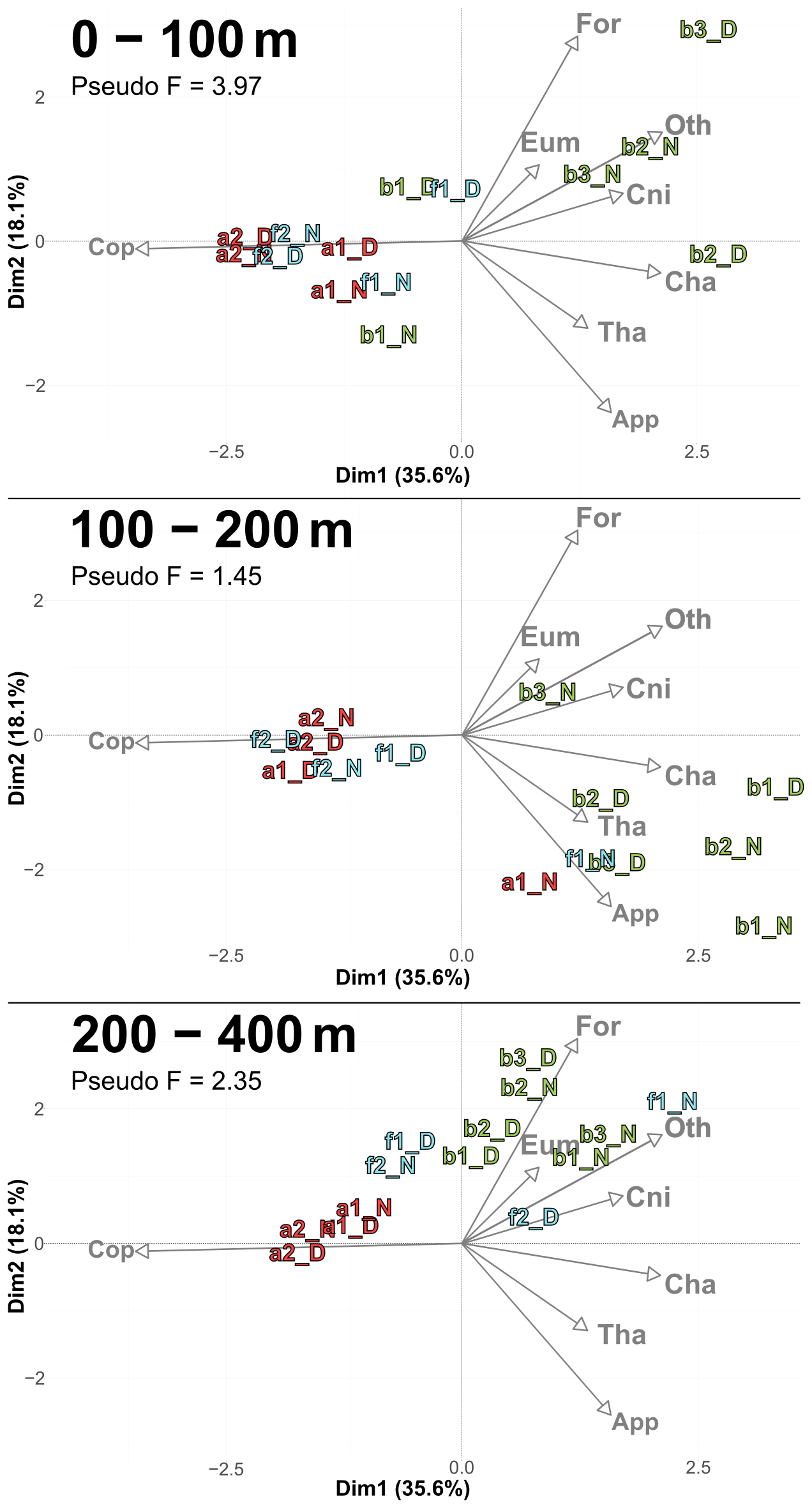
Figure 6 PCA_Community illustrating the composition of communities, based on relative concentration data (Hellinger transformation) from all stations for each reconstructed layer. The axis computed for 0–400 m were used for the three layers. Colors refer to the water mass (red for A, green for B, cyan for F and violet for M). In 0–100 m: stations a2_N and f2_D overlap at dim1 = −2.3 and dim2 = −0.3. In 100–200 m: stations a2_D and 2_D overlap at dim1 = −2 and dim2 = −0.1; f1_N and b1_D overlap at dim1 = 1.9 and dim2 = −1.8. In 200–400 m: stations a1_D and a2_N overlap at dim1 = −1.8 and dim2 = 0.3.

3.4.2 Comparison of the community composition between the front and adjacent waters

The relative concentrations of taxonomic groups across all stations, sorted by water mass and averaged across the three sampled layers, were used to compare the community compositions (Fig. 7). The results clearly revealed that the front appeared very similar to water mass A with copepod concentration progressively decreasing from A to F to B. To further investigate these observations, a PERMANOVA was conducted on the community composition. No significant difference was found between A and F (p=0.312). However, significant differences were observed between B and F (p=0.038) and between A and B (p = 0.006). For copepods, significant differences were found between all pairs of water masses and for both transects, as determined by an ANOVA, except between F and A (p = 0.406 for the first transect and p = 0.459 for the second transect). For other groups, significant differences were observed only for Other_Organisms between B and A for both transects and between F and B for the second transect.

Figure 8 illustrates the theoretical community distribution at the front, derived from a combination of communities from water masses A and B (Sect. 2.8.3). The positioning of theoretical front stations (f_t) is displayed within the PCA_Community of Fig. 6 (Fig. 8a). For the first transect (Fig. 8b), the α value (in Eq. 5) was low for the 0–100 m and 200–400 m layer (respectively 0.24 and 0.17) but high for the intermediate layer (0.75). This suggests that the front was influenced by processes other than just the dynamics of water masses, for instance DVM through the 100–200 m layer. For the second transect, α was close to 1, even equal to 1 for the deeper layers, indicating that the front was very similar to water mass A (Fig. 8c).

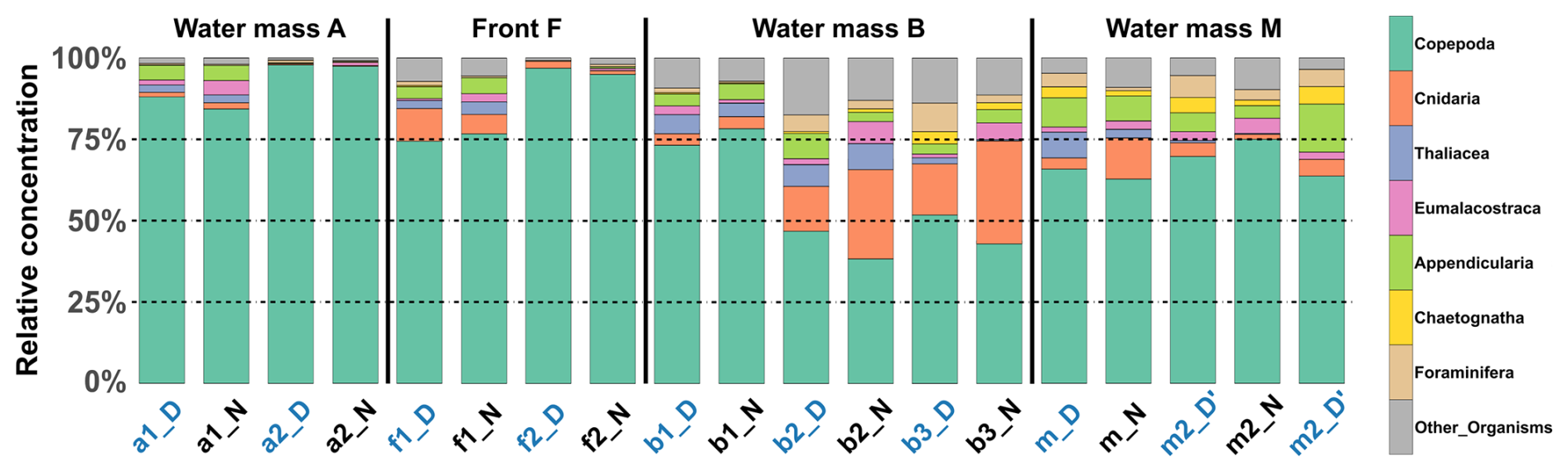
Figure 7 Relative concentration of taxonomic groups across all stations. Sorted by water mass and averaged across the three sampled layers at each station. Station name colors indicate the period of the day (blue: midday; black: midnight).

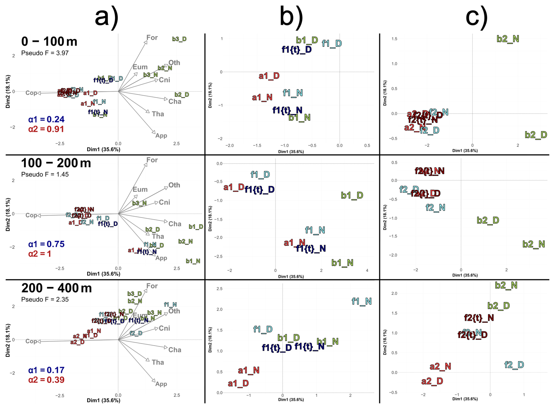
Figure 8 (a) PCA_Community illustrating the composition of communities, based on relative concentration data (Hellinger transformation) from all stations for each reconstructed layer (same as figure 6). The closest theorical f_t of each observed f is plotted, with the corresponding α1 and α2 values of each f_t's couple for the 1st and 2nd transect, respectively. (b) Zoom for the stations of the 1st transect. (c) Zoom for the stations of the 2nd transect. In (c), in 0–100 m stations a2_D, a2_N, f2_D, f2_N, f2{t}_D and f2{t}_N overlap at dim1 = −2.2 and dim2 = −0.2. In 100–200 m stations a2_N and f2{t}_N overlap at dim1 = 1.4 and dim2 = 0.2; a2_D, f2_D and f2{t}_D overlap at dim1 = −1.8 and dim2 = −0.4. In 200–400 m stations f2_N and f2{t}_D overlap at dim1 = −0.4 and dim2 = 1.

A notable feature is the position of f_t stations compared to observed f stations within the reduced PCA space. Focusing on the first transect (Fig. 8b), observed f stations appeared displaced relative to the f_t stations, being positively shifted along axes 1 and/or 2. To examine these shifts, we reconstituted the theoretical concentrations at these f_t stations and then compared them to those at the f stations. In the 0–100 m layer, the observed shift was driven by a 103 % higher concentration of Cnidaria at the front relative to the expected value at f_t, while all other groups declined (average decline of 49 %). In the 100–200 m layer, the discrepancy between f and f_t was explained by a 73 % higher concentration of Foraminifera at f, while all other groups decreased (average decline of 47 %). In the 200–400 m layer, the shift was explained by a pronounced 458 % higher concentration of Cnidaria and 217 % higher concentration of Foraminifera at f compared to f_t , while other groups increased by 21 % on average.

In contrast, the second transect had much higher alpha values, which means a strong similarity between water mass A and F, with a strong domination of copepods in both water masses (Fig. 8c). Thus, deviations between f_t and f were very low and could not be analyzed.

3.4.3 Size and taxonomic composition of copepods

According to the PCA_Size (Fig. 9), copepod size structure differed most strongly in the 0–100 m layer, with stations a and f dominated by larger individuals (> 950 µm), whereas b stations were characterized by smaller ones. The b stations also displayed a more heterogeneous distribution. PCA_Size with stations m included as supplementary individuals is provided in Appendix (Fig. A5). As depth increased, size composition became more homogeneous, with all stations clustering near the PCA center, but slightly shifted toward larger sizes. Indeed, there was a decrease in Pseudo-F with depth, respectively 4.85, 1.13 and 0.98. This concentration near the PCA center and the decrease in Pseudo-F indicated a gradual decrease in variability among the deep stations, i.e., the differences between stations became less pronounced. This was also observed in the PCA_Community but it was more pronounced for copepod size composition.

Furthermore, to assess whether a finer taxonomic resolution of copepods could provide additional insights beyond the analysis of the whole zooplankton community (Sect. 3.4.1), we performed a PCA (Fig. A6). In this analysis, copepods were subdivided into seven categories, each accounting for more than 1 % of total copepod concentration (see in Table 4). This finer taxonomic resolution confirmed the similarity between water mass A and the front, which were differentiated from water mass B, as previously observed in PCA_Community.

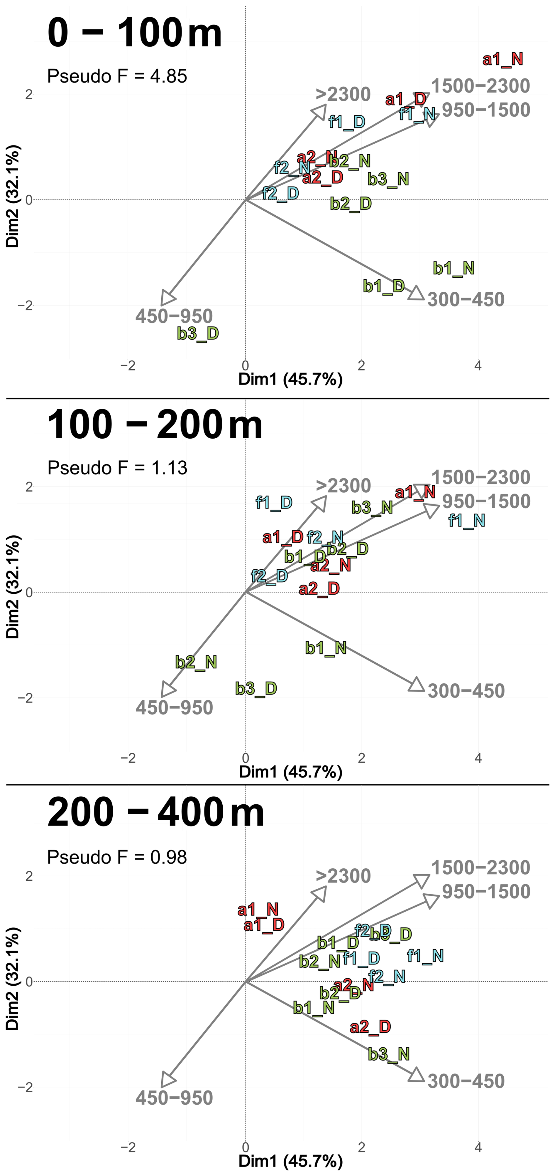
Figure 9 PCA_Size illustrating the body size composition of copepods, based on relative concentration data (Hellinger transformation) from all stations for each reconstructed layer. The size classes (in. µm) were defined according to those from NBSS. The axis computed for 0–400 m were used for the three layers. Colors refer to the water mass (red for A, green for B, cyan for F and violet for M). In 0–100 m: stations a2_N and b2_N overlap at dim1 = 1.8 and dim2 = 0.7. In 200–400 m: stations f2_D and b3_D overlap at dim1 = 2.3 and dim2 = 0.9; stations b2_D and a2_N overlap at dim1 = 1.9 and dim2 = −0.2.

4 Discussion

4.1 Hydrology, nutrients and zooplankton stocks in post-bloom NBF waters

Spatial differences between water masses A and B in late spring can be linked to the regional hydrology and ecosystem functioning of the NWMS during the post-bloom period (D'Ortenzio and Ribera d'Alcalà, 2009). Water mass A originates in the Liguro- Provençal area (NWMS), characterized by intense convection and mixing (Barral et al., 2021), high nutrient concentrations (Severin et al., 2017), and enhanced productivity (Mayot et al., 2017; Hunt et al., 2017) with the formation of a deep chlorophyll maximum around 50 m (Fig. A3; Lavigne et al., 2015; Doglioli et al., 2024). Water mass B, located in the southern part of the NBF, originates from the epipelagic waters of the Algerian basin. These waters are warmer and fresher than those of the NWMS, with virtually permanent stratification and a DCM (Deep Chlorophyll Maximum) deeper than 50 m (Fig. A3; Lavigne et al., 2015).

During the transitional post-bloom period (April-May) encountered during the BioSWOT-Med cruise, water mass A was nutrient-richer than water mass B with mean nitrate (phosphate) concentrations in the euphotic layer ranging from 0.64–1.27 (0.003–0.144) µM in A compared to 0.04–0.44 (below detection limit-0.003) µM in B. These contrasts also appeared at 500 m depth, nitrate (phosphate) concentrations ranging from 8.38–9.43 (0.34–0.40) µM in A compared to 7.49–8.89 (0.26–0.36) µM in B (Joel et al., 2025). Zooplankton stocks were higher in water mass A, dominated by large-sized copepods, whereas water mass B hosted smaller copepods and a more diversified community structure among non-copepod taxa (Figs. 5, 6, 9), consistent with Fernández de Puelles et al. (2004).

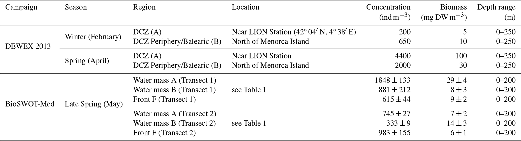
Mesozooplankton data from the two transects across the NBF during the BioSWOT-Med campaign can only be compared with a very limited number of previous observations, particularly in the vicinity of the front. The DEWEX (2013) campaigns (Conan et al., 2018), studied dense water formation and zooplankton dynamics during the winter-spring transition (Donoso et al., 2017). A comparison of zooplankton concentrations and biomasses between the two campaigns is presented in Table 3. Our biovolumes were converted to biomass using a DW/WW ratio of 10 %, assuming that 1 mg WW equals 1 mm³.

Table 3 Overview of concentrations and biomasses of zooplankton sampled during DEWEX (2013) and BioSWOT-Med campaigns. The depth range column indicates the vertical extent of the water layer considered for the calculation. DCZ stands for Deep Convection Zone. For BioSWOT-Med, values are given as the mean between day and night samples ± standard deviation.

4.2 Complexity of concurrent processes impacting zooplankton biomass distribution at front

The decline in zooplankton concentration at the front during the first transect (Fig. 3) may reflect specific hydrological and physical mixing characteristics of the NBF (Salat, 1995; Alcaraz et al., 2007), where dynamic turbulence and horizontal processes appeared less favorable for biomass accumulation. Although turbulence at front is known to enhance nutrient diffusion to phytoplankton, thereby promoting enriched food webs for zooplankton (Kiørboe, 1993; Estrada and Berdalet, 1997). It can also increase encounter rates between particles and consumers, thereby influencing community interactions (Rothschild and Osborn, 1988; Alcaraz et al., 1989; Saiz et al., 1992; Caparroy et al., 1998). Indeed, the front in our study area, sampled by Lagrangian drifters at 1 and 15 m depth (Demol et al., 2023), showed prevailing along-front deformation and patches of water mass convergence and divergence,

inducing variable vertical velocities up to approximately ± 1 mm s⁻¹ in the upper 15 m (Maristella Berta, personal communication, 2025). Moreover, ADCP transects (Petrenko et al., 2024) located the core of the front within the upper 100 m and across 20 km in width. Consequently, considering the frontal spatial scales, the divergence, and the magnitude and variability of vertical transport, we expect that our results do not reveal significant effects beyond 100 m depth and that mixing operates on shorter time scales than zooplankton development (several weeks to months). In a study of 154 glider-resolved fronts across the California Current System, Powell and Ohman (2015a) found that zooplankton biomass was often, though not always, enhanced, indicating variations in matchup of frontal duration and zooplankton development time. Finally, our campaign took place in late April to early May, corresponding to the post-bloom period (Fig. A3, Anthony Bosse, personal communication, 2025), when phytoplankton biomass was already too low to sustain optimal growth of specific zooplankton groups.

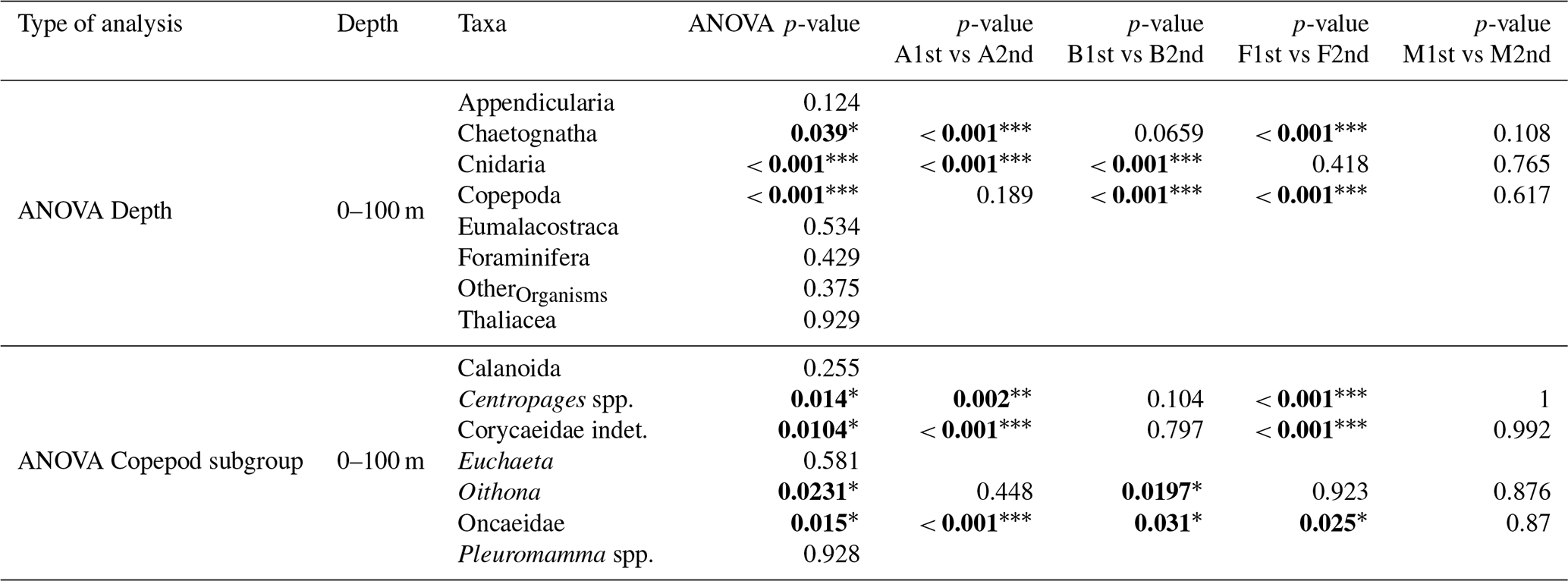
Table 4 Results of ANOVA tests (H₀: no difference in mean values between the first and the second transect) performed on the eight taxonomic groups and seven copepod subgroups (subgroups with a total concentration greater than 1 % of the overall copepod assemblage). Significant p-values (p<0.05) are shown in bold. The level of statistical significance is indicated by asterisks (^* p<0.05; ${}^{**}$ p<0.01; ${}^{***}$ p<0.001). For each significant ANOVA result, a Tukey’s Honest Significant Difference (HSD) test was applied to identify differences between the first and the second transect for each water mass (shown in the last four columns). For the 100–200 and 200–400 m layers, no significant differences were found.

4.3 Investigating the front: mixing zone or distinct community?

A fundamental question in this study was whether the front was a mixture of communities from water masses A and B, or if it hosted a distinct community with notably different concentrations of taxa. Our results indicated that the front was very similar to water mass A in several aspects: the taxonomic composition of zooplankton communities (Fig. 6), the body size distribution of copepods dominated by large individuals (Fig. 9), and the relative concentration of copepods, which decreases from A to F to B (Fig. 7). Moreover, in the 0–100 m layer, the shifts between the projections of f and f_t (Fig. 8) suggested a weaker influence of the front on Cnidaria and Foraminifera, likely because these groups were mainly represented by small forms (e.g., ephyrae) with limited swimming ability, which may have benefited from prey accumulation at the front. In contrast, the pronounced decrease in Thaliacea, largely composed of salp chains with strong vertical migration capacity, may reflect active avoidance of physical (e.g., turbulence) and trophic (e.g., high particle load) conditions associated with frontal regions.

The primary differences among taxonomic categories (Table 2) across the front were driven not by the most abundant groups, but by secondary groups: Cnidaria, Foraminifera, and Eumalacostraca for 0–100 m; Cnidaria and Foraminifera for 100–200 m. In other frontal studies, some taxa were found more abundant within the front than in adjacent waters (Molinero et al., 2008). Gastauer and Ohman (2024) similarly reported front-related increases in appendicularians, copepods, and rhizarians, underscoring that zooplankton community composition is shaped by taxon-specific responses. Biomass peaks also depend strongly on the taxa considered (Mangolte et al., 2023). However, in our analyses, we did not focus on a single taxon, but rather on groups of organisms (Table 2) or on the whole sampled mesozooplankton.

To answer our initial question, the results suggest that for the first transect, the front was indeed a mix of A and B communities, but it also showed higher concentrations of organisms such as Cnidaria, Foraminifera and Chaetognatha. For the second transect, the storm of the previous days may have altered the community structure (a hypothesis further discussed in Sect. 4.4), making it difficult to draw definitive conclusions.

4.4 Other potential factors affecting zooplankton structure

The method used to estimate concentrations in the 100–200 and 200–400 m layers relied on subtracting successive hauls (Sect. 2.5). While this approach was unavoidable given the sampling design, it introduced several potential sources of error: it is sensitive to zooplankton patchiness over short time scales and may produce inconsistencies between layers. Contamination during retrieval cannot be excluded, and in some cases, subtraction yielded negative values which were set to zero. To place our data in context, we compared our relative vertical distribution with reference values reported by Scotto di Carlo et al., 1984, who found approximately 57 % of zooplankton in 0–100 m, 27 % in 100–200 m, and 16 % in 200–400 m. In our dataset, mean relative concentrations were 46.2 ± 18.2 % in 0–100 m, 26.9 ± 18.5 % in 100–200 m, and 26.8 ± 15.5 % in 200–400 m. Although Scotto di Carlo et al. (1984) used a different net mesh size and did not separate day and night sampling, this comparison provides useful context. Therefore, concentrations in the upper 0–100 m layer were considered reliable. However, uncertainties remain in the reconstructed deeper layers, and results from these depths should therefore be interpreted with caution.

In addition to hydrological drivers, two processes may act as confounding factors when interpreting zooplankton community structure. First, DVM modifies the vertical distribution of many taxa. In our samples, taxonomic and size distributions of migrant zooplankton were more similar between the 0–100 and 100–200 m layers at night, and between the 100–200 and 200–400 m layers during the day (Sect. 3.3, Figs. 5, 9). This pattern reflects the well-documented behaviour of copepods and eumalacostracans performing large-amplitude DVM, in particular species of Pleuromamma, Euchaeta, and Heterorhabdus, which may migrate within the upper 400–500 m (Andersen and Sardou, 1992; Andersen et al., 2001b; Isla et al., 2015; Guerra et al., 2019). Thus, the 100–200 m layer appeared to act as a transitional zone.

Second, an intense windstorm occurred between the two BioSWOT-Med transects (NW winds, peaking on 2 May). While glider data indicated only a limited deepening of the mixed layer (from 15 to 30 m) and moderate changes in chlorophyll a fluorescence (no dilution of the DCM after the storm, Fig. A3), some changes in zooplankton composition in the 0–100 m layer may have reflected storm-induced mixing and dilution. Similar short-term effects of storms were previously reported in the NWMS, including increased nauplii production linked to adult spawning but reduced copepod biomass, and upward aggregation of nauplii and small-sized copepods in the upper 40 m (Andersen et al., 2001a; Andersen et al., 2001b; Barrillon et al., 2023). In our case, the comparison of concentrations between the two transects revealed significant differences in the 0–100 m layer, but not in deeper layer, therefore potentially linked to the storm (Table 4). In this surface layer, small and mid-sized copepods, chaetognaths, and cnidarians were the most affected, whereas large migrant copepods, such as Pleuromamma and Euchaeta, appeared only weakly impacted. A similar trend was observed for Calanoida, which includes both small and large, migrant and non-migrant species. Analyses of the whole planktonic community response to the storm (including phytoplankton) will be required to better understand the observed zooplankton changes.

However, because the two transects were 9 days apart and approximately 50 km apart, the present dataset does not allow storm effects to be unambiguously disentangled from general temporal or spatial variability. The storm should therefore be considered as one, but not exclusive, driver of the observed changes.

The observed variability in zooplankton concentrations over time and space underscores the complexity of concurrent processes acting at different scales, such as DVM or storm events interacting with the hydrological processes that create the front.

5 Conclusions

To our knowledge, this study represents the first detailed investigation of fine-scale zooplankton distribution in the NBF during late spring, linking fine-scale dynamics to mesozooplankton distributions. Our findings reveal that the NBF exhibited characteristics more akin to a boundary between water masses than a zone of pronounced biological accumulation. Key observations include the stratified vertical distribution of zooplankton communities, with distinct taxonomic compositions in the surface, intermediate, and deeper layers, and a progressive homogenization of community structure with depth. DVM was particularly evident, underscoring the dynamic nature of zooplankton behavior in relation to environmental gradients. Moreover, post-storm analyses highlighted the susceptibility of these communities to episodic weather events, which can disrupt established ecological patterns.

These results challenge generalized assumptions about the ecological role of oceanic fronts. They underscore the importance of high-resolution observations across horizontal and vertical spatial scales, consideration of short temporal processes, and precise taxonomic identification to fully understand the complexity of mesozooplanktonic communities in frontal zones.

Further trophic studies based on stable isotope ratios and the biochemical composition of zooplankton and phytoplankton size classes are still needed. Such studies would help to decipher trophic interactions in the frontal area, where nutrient input is driven by physical processes. In addition, our net sampling approach needs to be complemented by continuous measurement techniques, such as autonomous gliders, bioacoustics, and satellite data, together with in-situ sampling to better capture the spatial and temporal variability of these systems. This approach would enable a more comprehensive assessment of how physical and biological processes interact to shape zooplankton communities at oceanic fronts.

Appendix A

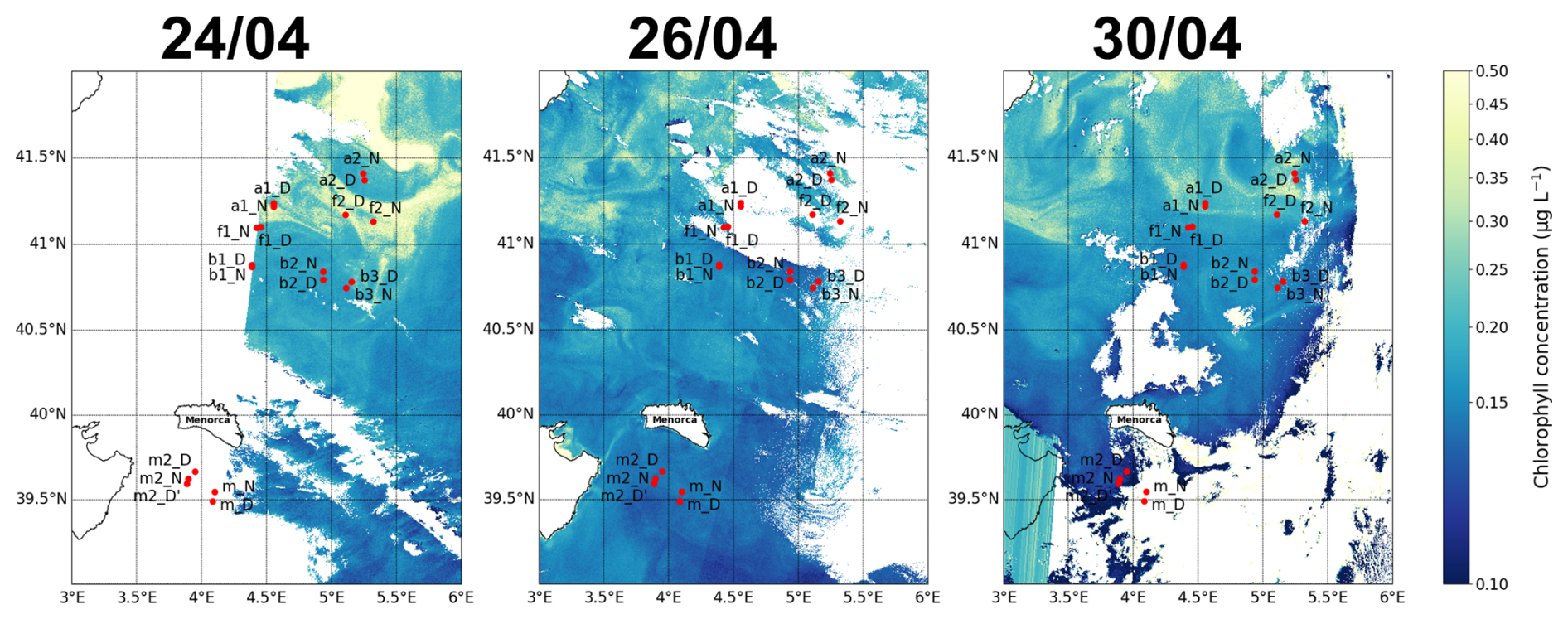
Figure A1 Maps of the sampling stations with surface chlorophyll concentration for 3 different days (as complement of Fig. 2).

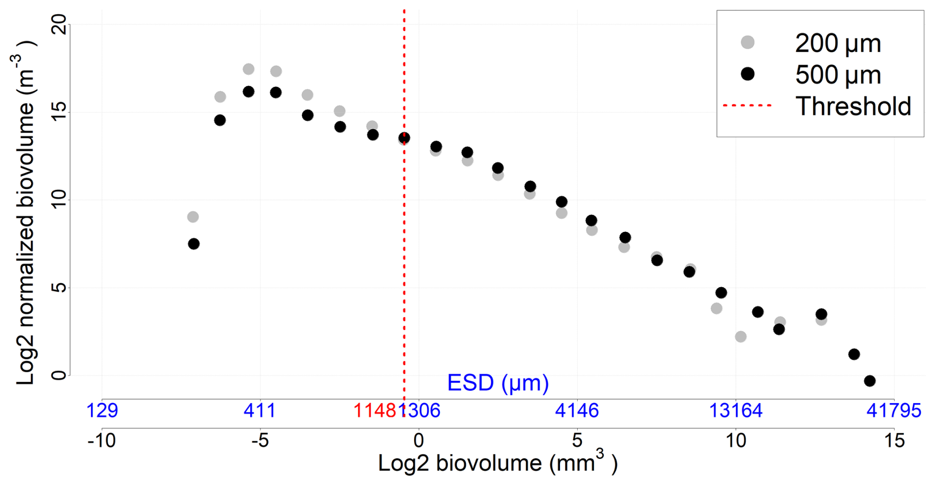
Figure A2 NBSS incorporating all data (all stations and depths) for each mesh size. The threshold value represents the organism size above which the 500 µm nets sample more efficiently than the 200 µm nets.

Figure A3 Total particles abundance, temperature, salinity, and fluorescence profiles.

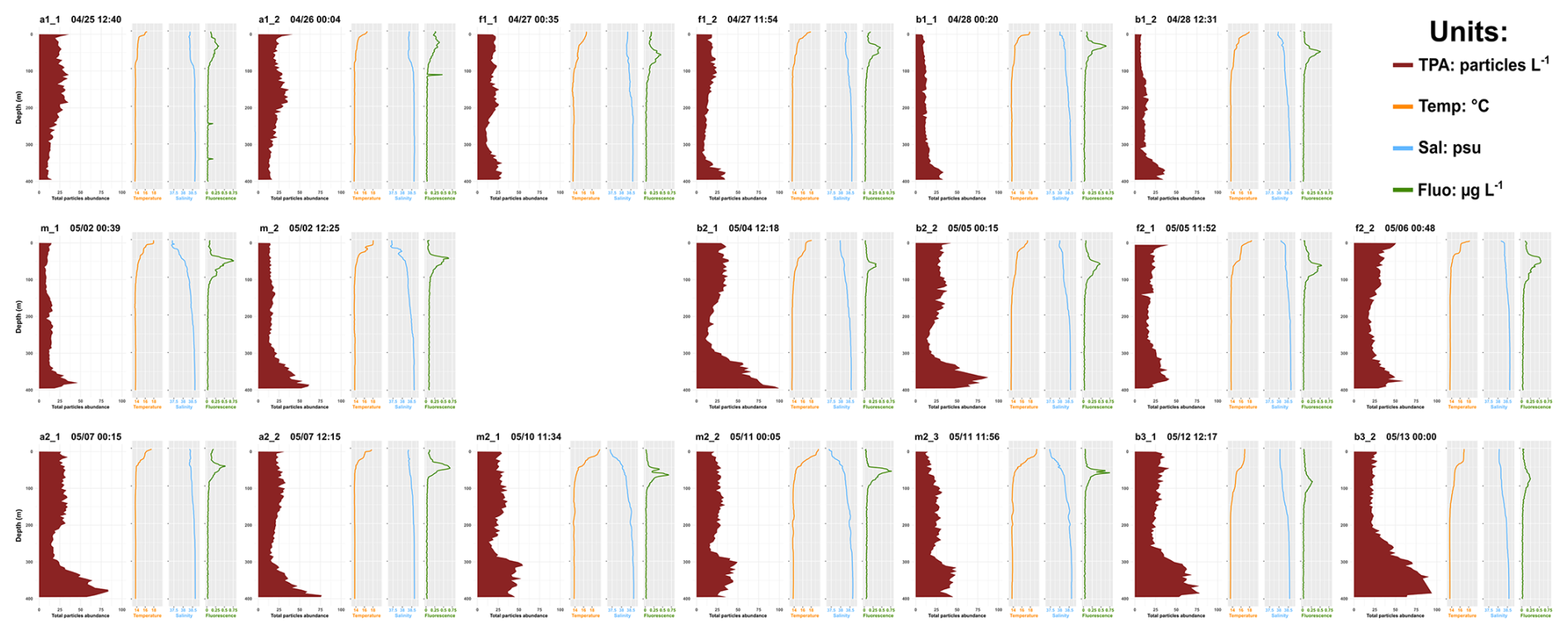
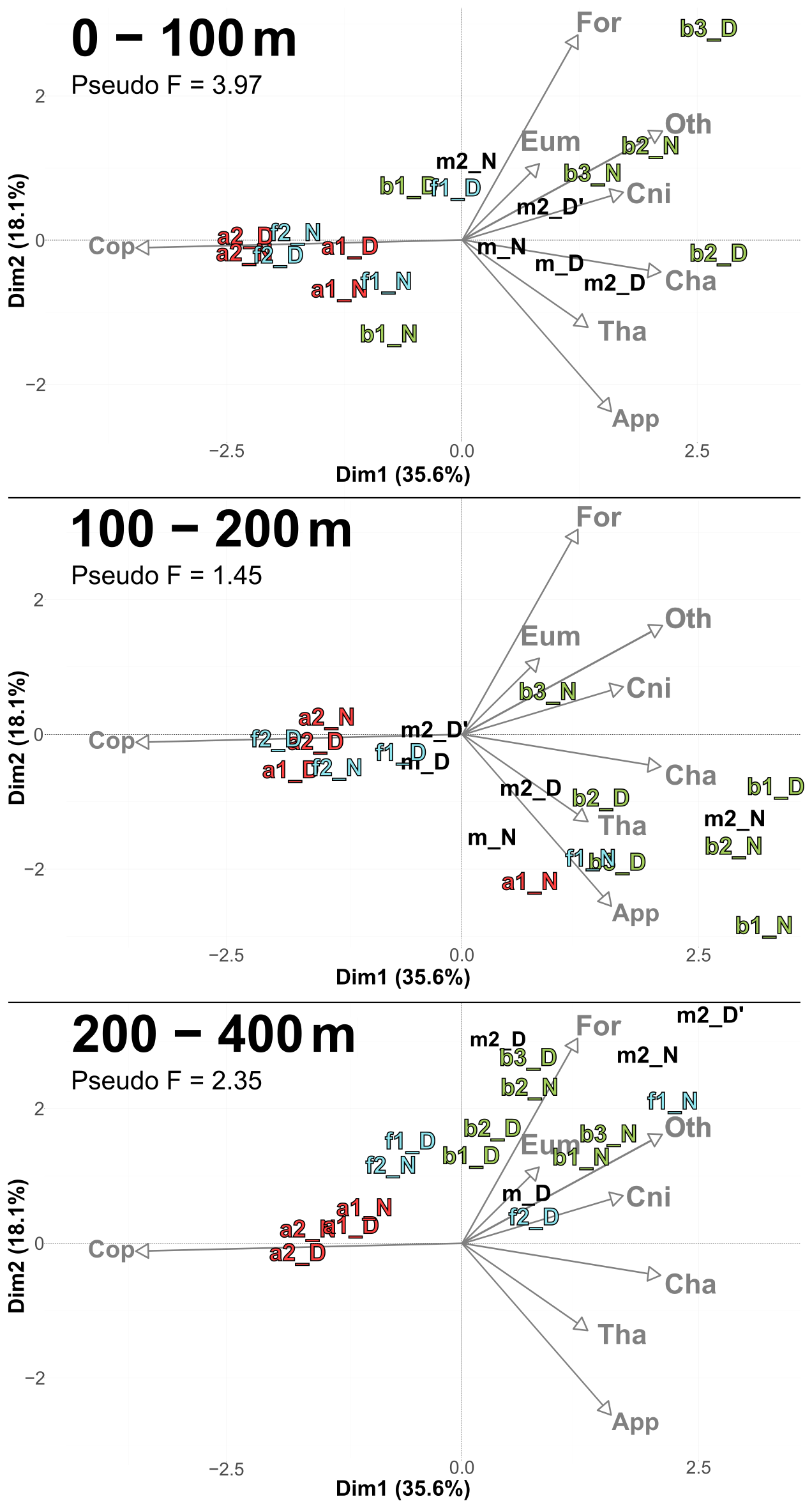
Figure A4 PCA_Community (same as Fig. 6) with m stations projected as supplementary individuals.

Figure A5 PCA_Size (same as Fig. 9) with m stations projected as supplementary individuals.

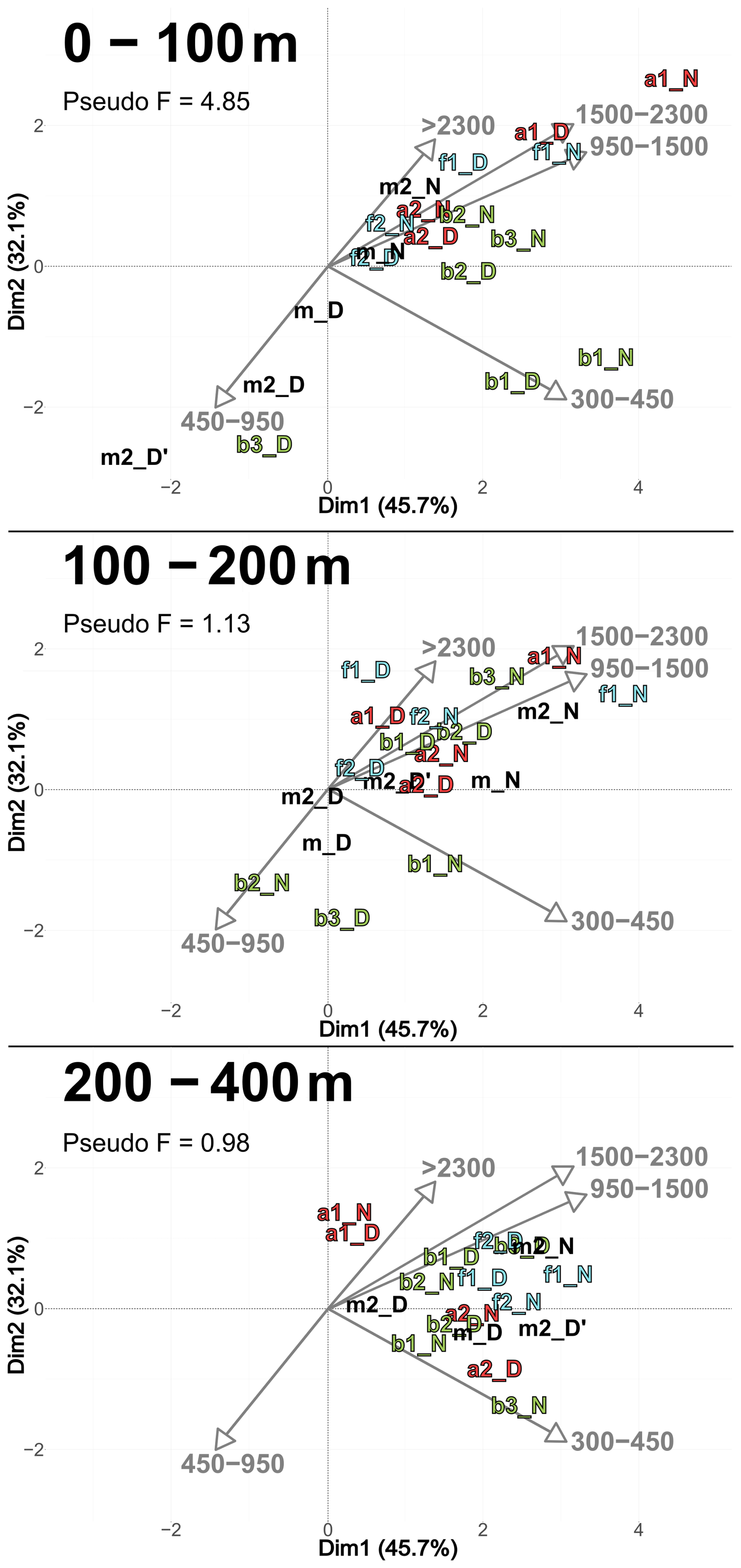
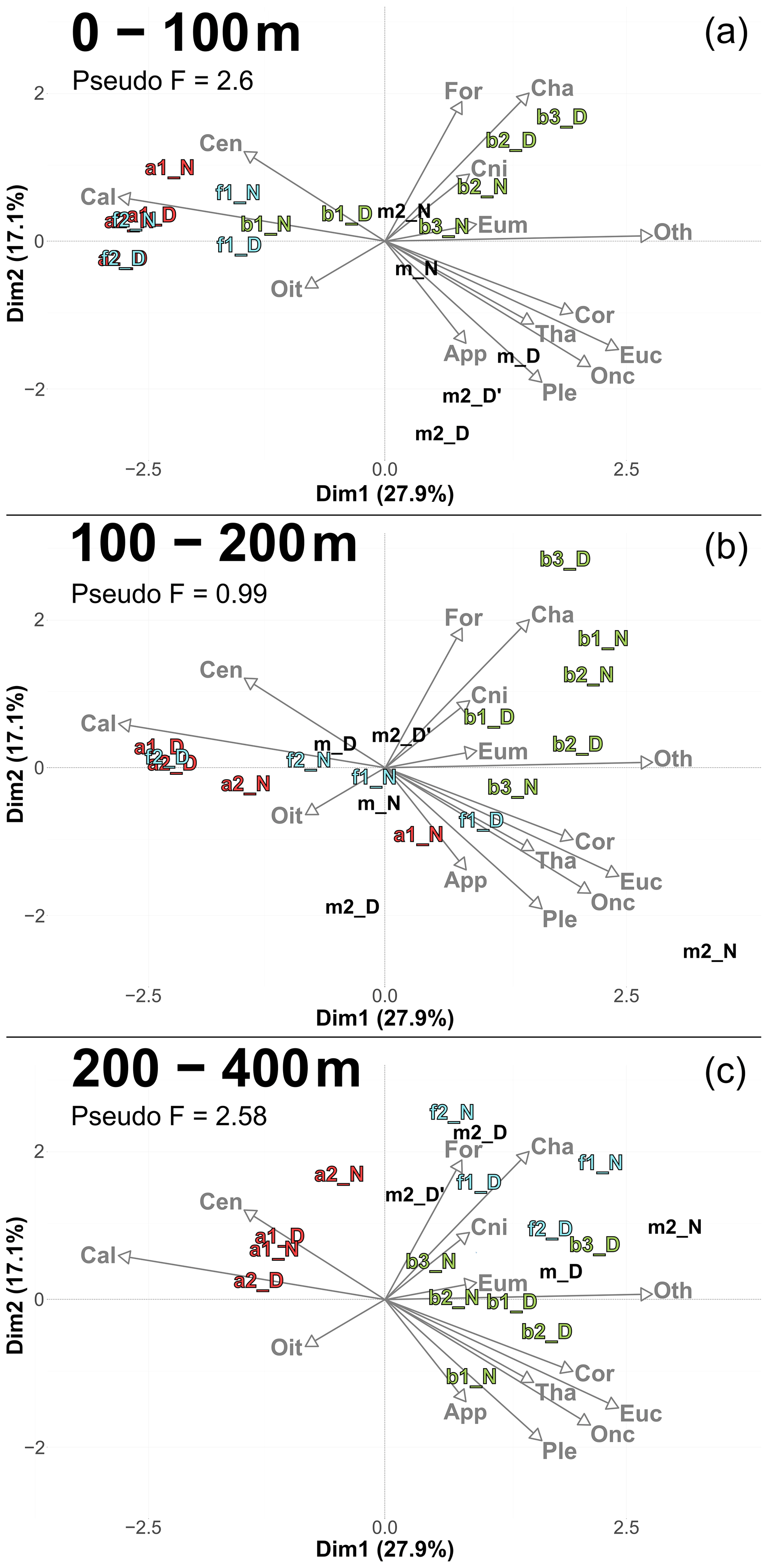
Figure A6 PCA illustrating the taxonomic composition of communities with copepods divided in seven copepod subgroups (subgroups with total concentration greater than 1 % of the overall copepod assemblage). Based on relative concentration data (Hellinger transformation) from all stations for each reconstructed layer (a) 0–100 m, (b) 100–200 m, (c) 200–400 m. The axis computed for 0–400 m were used for the three layers. Colors of station names refer to the water mass (red for A, green for B, cyan for F).