Understanding the resilient carbon cycle response to the 2014–2015 Blob event in the Gulf of Alaska using a regional ocean biogeochemical model

Marine heatwaves (MHWs), characterized by anomalously high sea surface temperatures, are increasing in frequency and intensity and strongly impact ocean circulation, biogeochemistry, and marine ecosystems. During the 2014–2015 MHW (commonly called the Blob) in the NE subarctic Pacific, moored observations at Ocean Station Papa (OSP; 145° W, 50° N) showed a moderate decrease in oceanic pCO₂, contrary to the increase expected from warming-induced solubility reduction alone. Using a regional model that reproduces the observed pCO₂ variability and trend at OSP, we show that this decline resulted from a decrease in dissolved inorganic carbon (DIC) supply that outweighed the warming-driven increase in pCO₂. The DIC reduction was primarily caused by weakened vertical transport associated with enhanced upper-ocean stratification and reduced Ekman pumping prior to the onset of the Blob, which suppressed the upwelling of DIC-rich subsurface waters. Horizontal transport also contributed locally, particularly at OSP. These results demonstrate that anomalous physical circulation, rather than biological processes, was the primary driver of the enhanced CO₂ uptake during the Blob and highlight the importance of resolving physical transport mechanisms when assessing carbon cycle responses to extreme warming events.

1 Introduction

Approximately 25 % of historical anthropogenic carbon emission has been absorbed by the oceans (Friedlingstein et al., 2022), and the North Pacific is one of the major regions for ocean carbon uptake (Takahashi et al., 2009). The carbon exchange between the atmosphere and ocean is closely related to ocean temperature through its influences on the solubility of carbon dioxide (CO₂) in seawater. In recent years, anomalously high ocean temperatures, known as marine heatwaves (MHWs; Hobday et al., 2016), have been frequently observed. These events are defined by prolonged periods of unusually high sea surface temperature (SST) anomalies and their intensity. With the ongoing progression of global warming, the frequency and intensity of MHWs have been increasing (Frölicher et al., 2018; Oliver et al., 2018). In particular, the persistent MHW that occurred in the subarctic NE Pacific from the winter of 2013 to 2015, known as the Blob (Bond et al., 2015), had severe impacts on surrounding ecosystems (Cavole et al., 2016; Smale et al., 2019) and fisheries (Barbeaux et al., 2020). This anomalously high ocean temperature was attributed to weaker surface winds, which reduced ocean surface heat loss, and weakened horizontal and vertical mixing (Bond et al., 2015; Di Lorenzo and Mantua, 2016).

Biogeochemical variables are also impacted by MHWs. In particular, low-oxygen and acidification become more pronounced during MHWs (Gruber et al., 2021; Burger et al., 2022; Li et al., 2024b). These changes are driven by alterations in ocean circulation due to changes in wind and air–sea interactions associated with atmospheric anomalies that induce the MHWs, and also by the direct effects of high temperatures (e.g. enhanced stratification, reduced solubility, and changes in biological activity). During the Blob, both surface dissolved oxygen and inorganic carbon (DIC) were significantly decreased partly due to reduced solubility caused by increased water temperatures (Mogen et al., 2022; based on ocean model outputs from NorESM and MRI simulations). Franco et al. (2021) showed a decrease in surface DIC during the Blob using in situ time-series measurements.

For the air–sea CO₂ exchange, the uptake in the North Pacific decreased by 29 ± 11 % during persistent MHWs mainly due to the direct effect of increased water temperature (Mignot et al., 2022). However, this reduction in ocean carbon uptake is primarily driven by the substantial increase in oceanic CO₂ outgassing in the tropical Pacific. Focusing on the subarctic regions, the oceanic CO₂ uptake increased during the MHWs. For example, mooring data from Ocean Station Papa (OSP; 50° N, 145° W) in the eastern North Pacific, which is one of the longest-running observation sites, showed low surface DIC and oceanic partial pressure of CO₂ (pCO₂) during a more recent MHW (Kohlman et al., 2024). In the Gulf of Alaska (GOA), air–sea CO₂ flux exhibited a negative anomaly (stronger ocean uptake) of approximately 45 % relative to the climatological monthly means during the Blob based on a machine-learning based reconstruction (Duke et al., 2023). The enhanced ocean carbon uptake is caused by the decrease in oceanic pCO₂ in the subarctic North Pacific, which is driven by the effects of reduced surface ocean DIC. However, the processes responsible for this DIC reduction is not fully understood (Mignot et al., 2022; Li et al., 2024a). Furthermore, estimates of oceanic pCO₂ changes derived from observation-based products are subject to considerable uncertainty, as observational data in the subarctic North Pacific are temporally and spatially sparse. Consequently, discrepancies among data products restrict the robustness of their assessments (Li et al., 2024a).

To elucidate the mechanisms by which the MHWs lead to the observed changes in oceanic pCO₂ and air–sea CO₂ fluxes, numerical models can provide the carbon mass balance and exploring underlying physical and biogeochemical processes. Physical processes that control the regional ocean circulation, biogeochemical cycling, and air–sea gas exchanges often occur at scales smaller than several tens of kilometres, which remain unresolved in global earth system models (Gruber et al., 2021). In the subarctic NE Pacific, reproducing the full variability of oceanic pCO₂ in models is complicated by boundary currents and eddies that transport macro- and micro-nutrients, alkalinity and DIC. A previous study using a coarse resolution model (Mckinley et al., 2006) has shown that although models captured the variability of individual components of oceanic pCO₂ on seasonal and interannual timescales, they have not fully reproduced the total variability of oceanic pCO₂, and their ability to simulate the temporal patterns of air–sea CO₂ fluxes remains limited.

There are several regional modeling studies exploring biogeochemical processes in the GOA. Coyle et al. (2012) developed regional, biogeochemical simulations for the northern GOA based on the ROMS circulation model with the horizontal resolution of 3 km from 2001 to 2004 focusing on the coastal regions. The biogeochemical model component is based on the GOANPZ model (Hinckley et al., 2009). The model reproduced the spring phytoplankton bloom from the continental shelves to the open ocean. This model subsequently was used to analyze ocean acidification with the inclusion of carbonate chemistry (Siedlecki et al., 2017). Hauri et al. (2020) developed a hindcast simulation for the similar northern GOA domain. They also used the ROMS physical model with 4.5 km horizontal resolution. The biogeochemical component is based on the COBALT biogeochemistry model (Stock et al., 2014) with specific modifications to capture coastal ecosystems. Following these previous studies, we constructed a regional biogeochemical and carbon cycle model for the GOA. The model has been validated against a suite of physical and biogeochemical observations (Ito et al., 2026) This study expands the model to include a validated carbon cycle component. The simulated temporal variability of oceanic pCO₂ is validated with the NOAA (Pacific Marine Environmental Laboratory's Ocean Climate Stations and Carbon groups) mooring at OSP (Emerson et al., 2011; Cronin et al., 2015). The model outputs are used to understand the underlying mechanisms and to quantify the changes in oceanic pCO₂ in this critical carbon sink during the Blob. This paper includes the description of the model and the observational data used for model validation (Sect. 2), and the results of oceanic pCO₂ variations during the Blob and its causes (Sect. 3). Section 4 discusses the associated changes in CO₂ flux, the potential impacts of high ocean temperature anomalies on the regional carbon cycle, their effects on the broader ocean basin, and possible future implications. Finally, Sect. 5 summarizes the main findings of this study.

2 Data and Methods

2.1 Model description

The regional ocean circulation and biogeochemistry model used in this study followed the configuration described in Ito et al. (2026), thus only a brief description was provided here, while full details can be found in their paper. The model was based on MITgcm (Marshall et al., 1997a, b) combined with an ocean biogeochemical model, Biogeochemistry with Light, Iron, Nutrients and Gases (BLING) version 2 (Dunne et al., 2020) including 10 tracers, DIC, alkalinity, O₂, PO₄, NO₃, dissolved Fe, silica, dissolved organic P, and dissolved organic N. The model was driven by 3-hourly averaged atmospheric variables from the JRA-55-do reanalysis data (Tsujino et al., 2018), including the surface air temperature, humidity, 10 m wind stress, precipitation (both rain and snow), river runoff, and downward shortwave and longwave radiation. The earlier simulations of Ito et al. (2026) included a positive bias in sea surface salinity (SSS) of approximately +0.2 psu. To maintain SSSs close to the observations, we applied Newtonian relaxation to SSS toward monthly climatology from World Ocean Atlas 2023 (Reagan et al., 2024) with a restoring timescale of 30 d in the surface grid box of 10 m thickness. The model had a horizontal resolution of 10 km with 42 vertical layers on a latitude-longitude z-level grid. The bathymetry was generated by interpolating the ETOPO2 global 2 min resolution topography dataset. The model domain had a southern open boundary at 42 N and a western open boundary at 160° W. Vertical mixing was parameterized using the K-profile Parameterization (KPP) scheme (Large et al., 1994) as implemented in MITgcm. The default configuration, including the non-local convection term, was used for this study. KPP diffusivities were applied to momentum and all tracers. A sea ice model, implemented using the MITgcm sea ice package (Losch et al., 2010) and coupled to the ocean component, was used to represent sea ice dynamics and thermodynamics, as well as their influence on surface heat, freshwater, and momentum fluxes.

Both the initial and boundary conditions in our model also followed Ito et al. (2026). Open boundary conditions were set to the climatological values from GLODAPv2 (Lauvset et al., 2022) for most of the biogeochemical properties. However, for DIC, the open boundary conditions included time-dependent anthropogenic carbon rather than climatology. Temporal changes in DIC due to anthropogenic influences were imposed according to the rate of change in atmospheric CO₂ fractions measured at the Mauna Loa Observatory (Keeling et al., 2001) and its spatial structure was set to the anthropogenic carbon estimates from the GLODAPv2. The model integration was performed through 2017, and the physical open boundary conditions were taken from the oceanic reanalysis data of Simple Ocean Data Assimilation (SODA) version 3 (Carton and Giese, 2008; Carton et al., 2018).

Several biogeochemical parameters were adjusted to improve the model representation of the carbon cycle. These modifications primarily involved processes related to strength of photosynthesis and remineralization. The modeled default parameters for photosynthetic rates caused excessively high rates in coastal waters, resulting in unrealistically elevated primary production. To address this, the self-shading effect of phytoplankton was turned on, which regulated the light available for phytoplankton growth in the highly productive coastal waters. The bio-optical parameterization of Manizza et al. (2005) was used in our configuration but the background attenuation coefficient in this bio-optical model was reduced to one-quarter of its default value to re-calibrate the net primary production (NPP). Furthermore, the simulated oceanic pCO₂ was highly sensitive to the production of organic matter and the subsequent remineralization. A key factor was the export ratio which determines the fraction of NPP that sinked as particulate organic matter from the surface layer and was subsequently recycled in the subsurface waters. Among the relevant parameters, the partitioning of particulate organic versus dissolved organic matter exerted a particularly strong influence on the representation of oceanic pCO₂. To better capture observed oceanic pCO₂, we adjusted this parameter so that 30 % of NPP is converted to dissolved organic matter, compared with a default value of 10 %, which meaned that more organic matter was recycled in the surface layer than the default configuration.

2.2 Observations

To evaluate the model skills in reproducing the observed oceanic pCO₂, SeaFlux data (Fay et al., 2021) were used for spatial comparisons, and NOAA CO₂ mooring data (Emerson et al., 2011; Cronin et al., 2015) were used for temporal comparisons at OSP. SeaFlux data consisted of six global observation-based gridded products that reconstruct spatiotemporally continuous estimated of air–sea CO₂ fluxes using different gap-fill methods on the surface oceanic pCO₂ observations. Because the spatial resolution of SeaFlux was one degree in latitude and longitude, our model output was remapped to the same resolution using nearest-neighbour interpolation for comparison. In June 2007, a surface CO₂ mooring time series was initiated at OSP by Steve Emerson for the study of North Pacific Carbon Cycle, and the mooring observation has been continued by NOAA Office of Climate Observations. This data provided both physical and biogeochemical variables. For comparison with the model, temperature, salinity, and both oceanic and atmospheric pCO₂ data were obtained from the mooring dataset archived at https://www.ncei.noaa.gov/access/ocean-carbon-acidification-data-system/oceans/Moorings/Papa_145W_50N.html (last access: 1 October 2025). For comparison, OSP in the model was represented by averaging all grid points within a 24 km radius of 50° N, 145° W.

Model skill was further evaluated against the spatial patterns of monthly SST anomalies from the OISST dataset (0.25° resolution; Reynolds et al., 2007; Huang et al., 2021) and the HadISST dataset (1° resolution; Rayner et al., 2003).

2.3 Analysis methods

The oceanic pCO₂ anomalies were decomposed as:

$$\begin{array}{}\text{(1)}& \begin{array}{rl}\mathit{\delta }p{\mathrm{CO}}_{\mathrm{2}}& \approx {\displaystyle \frac{\partial p{\mathrm{CO}}_{\mathrm{2}}}{\partial T}}\mathit{\delta }T+{\displaystyle \frac{\partial p{\mathrm{CO}}_{\mathrm{2}}}{\partial S}}\mathit{\delta }S\\ & +{\displaystyle \frac{\partial p{\mathrm{CO}}_{\mathrm{2}}}{\partial {\mathrm{DIC}}^{\ast }}}\mathit{\delta }{\mathrm{DIC}}^{\ast }+{\displaystyle \frac{\partial p{\mathrm{CO}}_{\mathrm{2}}}{\partial {\mathrm{ALK}}^{\ast }}}\mathit{\delta }{\mathrm{ALK}}^{\ast }\end{array}\end{array}$$

where oceanic pCO₂ was a function of SST (T), SSS (S), sea surface salinity-normalized DIC (DIC^*) and sea surface salinity-normalized alkalinity (ALK^*). The contributions of these four variables to the oceanic pCO₂ anomalies were calculated using the Python toolbox PyCO2SYS (Humphreys et al., 2022) version 1.8.3. For the input variables, DIC and alkalinity were normalized to a salinity of 35 to eliminate the influence from evaporation and dilution (Keeling et al., 2004). The partial derivatives were evaluated at each time step by perturbing each variable independently while holding the others constant. For this calculation, the constants were set to the median of the temporal variations, and the perturbations were applied with an amplitude equal to the standard deviation. The results were obtained for each grid, and the values at OSP were as follows: $\partial p{\mathrm{CO}}_{\mathrm{2}}/\partial T=\mathrm{15.27}$ µatm °C⁻¹, $\partial p{\mathrm{CO}}_{\mathrm{2}}/\partial S=\mathrm{25.26}$ µatm psu⁻¹, $\partial p{\mathrm{CO}}_{\mathrm{2}}/\partial {\mathrm{DIC}}^{\ast }=\mathrm{2.15}$ µatm (µmol kg⁻¹)⁻¹, $\partial p{\mathrm{CO}}_{\mathrm{2}}/\partial {\mathrm{ALK}}^{\ast }=-\mathrm{1.76}$ µatm (µmol kg⁻¹)⁻¹. In the oceanic pCO₂ decomposition analysis, all input variables were detrended and deseasonalized using the STL function from the statsmodels.tsa.seasonal module in Python.

3 Results

3.1 Observational evidence of ΔpCO₂ during marine heatwave

To assess the magnitude of the SST anomalies during the Blob and evaluate whether the model was consistent with the observations, we compared the observed SST anomaly fields (Fig. 1). Both OISST and HadISST showed positive temperature anomalies across the GOA. The SST anomalies in OISST were larger than those in HadISST, particularly in the southeastern region. The modeled SST anomalies showed good agreement with both OISST and HadISST in terms of their spatial patterns and overall amplitudes. Given this consistency, the model robustly represented the observed SST anomalies, suggesting that model biases in SST were unlikely to influence the interpretation of the SST-driven component of oceanic pCO₂.

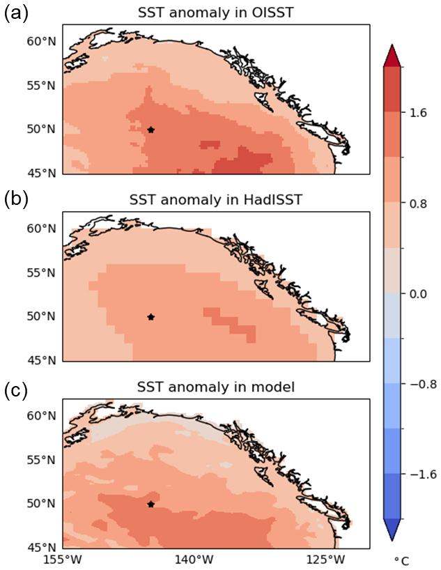
Figure 1 Annual SST anomaly during Blob (2014–2015) relative to 2010–2017 from (a) OISST, (b) HadISST, and (c) the model. The star indicates where OSP is located.

Seaflux pCO₂ data revealed the basin-scale surface oceanic pCO₂ climatologies and anomalies during the Blob. Annual mean climatology (2010–2017) showed negative ΔpCO₂ (oceanic pCO₂ is smaller than atmospheric pCO₂), indicating that the entire domain of the model acted as a sink for atmospheric CO₂ in the climatological mean field (Fig. 2a). Positive SST anomalies were expected to reduce CO₂ saturation in the ocean and consequently increase oceanic pCO₂. However, observation-based data showed a decrease in oceanic pCO₂, accompanied by a larger amplitude of ΔpCO₂ than non-heatwave conditions during the Blob (Fig. 2c). This indicated that the surface ocean absorbed more CO₂ from the atmosphere during the Blob (2014–2015), especially in the central GOA (blue areas in Fig. 2c). This trend contrasted with the rising SST, which increases oceanic pCO₂ and reduces ocean carbon uptake (Fig. 2d). An estimated contribution from the positive SST anomalies on ΔpCO₂ should result in an increase in ΔpCO₂ across the entire region (Fig. 2d). Therefore, elevated SST cannot account for the observed decrease in ΔpCO₂ during the Blob.

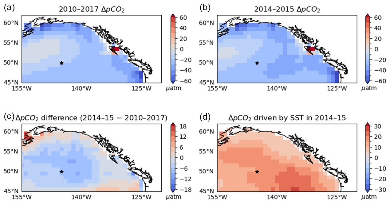
Figure 2 ΔpCO₂ (oceanic ΔpCO₂ minus atmospheric ΔpCO₂): (a) mean over 2010–2017, (b) mean during the Blob period from 2014-2015, (c) difference between (b) and (a), and (d) the component driven by SST changes during the Blob in SeaFlux. The SST-driven oceanic pCO₂ in (d) is calculated as the difference between pCO₂ computed under climatological mean conditions (2010–2017 mean SST and SSS from SODA version 3.4.2, and DIC and alkalinity from GLODAPv2) and pCO₂ computed using SST from 2014–2015, while keeping the other variables fixed at their climatological values, with PyCO2SYS. Blue indicates CO₂ uptake by the ocean, and red indicates CO₂ outgassing to the atmosphere. The star in each panel marks the location of OSP.

3.2 Model validation

Before using the model to address the underlying mechanism behind the oceanic pCO₂ decreases during the Blob, the ability of the model to reproduce existing observations must be evaluated. We first examined the model output for ΔpCO₂. Consistent with the observations, the model indicated that increasing SST cannot account for the changes in oceanic pCO₂ under the Blob, not only at OSP but across the entire GOA (Fig. 3). Compared to the observations (Fig. 2), ΔpCO₂ driven by SST under the Blob in the model was approximately 5 µatm higher around OSP. Despite the moderate overestimation in thermal-driven pCO₂ anomaly, the modeled ΔpCO₂ showed a significant decrease across the central GOA, consistent with the SeaFlux dataset and the mooring observation at OSP. This consistency was underscoring the robustness of the modeled response. Throughout the region, the effect of warming-induced increase in the oceanic pCO₂ was offset by the oceanic pCO₂ reduction driven by decreased DIC, which was consistent with the previous work by Kohlman et al. (2024).

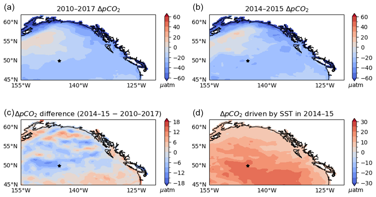
Figure 3 Same as Fig. 2 but for the model results.

Compared to the ensemble mean of the time-averaged oceanic pCO₂ from 2010 to 2017 in the SeaFlux dataset, the spatial correlation between SeaFlux and the model was moderately positive (r=0.30), and the model generally reproduced the broad climatological spatial distribution of the observed SeaFlux oceanic pCO₂ (Fig. 4a, c). The model overestimated oceanic pCO₂ in the northwestern area, which likely arised from model circulation biases in this region. Compared to satellite observations, the model had slightly weaker horizontal geostrophic flow, and the core of the subpolar circulation was shifted northward (Ito et al., 2026). The modeled vertical stratification was slightly weakened relative to the climatological observations, and this weak stratification bias led to a higher oceanic pCO₂ in the model. To evaluate the uncertainties in the SeaFlux dataset, variability among the different observational ensembles must be considered. In the open ocean, modeled oceanic pCO₂ was within the range of SeaFlux ensemble variability (Fig. 4b, d). Therefore, in most areas, the model was within the uncertainty bounds of the observation-based oceanic pCO₂.

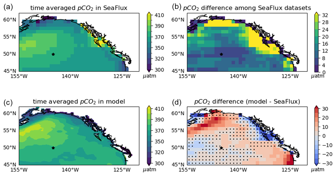
Figure 4 Comparison of oceanic pCO₂ distributions, averaged over 2010–2017, between the model and SeaFlux. The star in each panel indicates the location of OSP. Dots in (d) indicate the grid points where the modeled climatology falls within the range of differences among the SeaFlux ensemble datasets.

The model also reproduced the temporal variation in oceanic pCO₂ to a reasonable extent. Compared with the mooring time series at OSP, the model captured the observed variability and magnitude in both biogeochemical and physical variables (Fig. 5). For oceanic pCO₂, the model reproduced a statistically significant fraction of the mooring pCO₂ variability (r=0.44, normalized-RMSE = 1.01), and fell within the spread of the SeaFlux ensemble data. During the Blob, both the mooring observations and model showed pronounced decline in oceanic pCO₂. Correspondingly, ΔpCO₂, which represented the difference between the black or blue line and the orange line in Fig. 4a also decreased. The model slightly overestimated SSS (∼ 0.1 psu) compared to the mooring during the Blob, but this did not significantly compromise the stratification in the model, because the density was primarily governed by sea water temperature in this region.

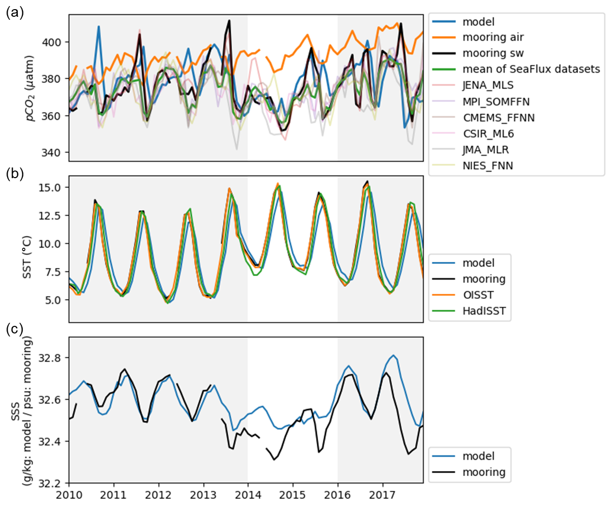
Figure 5 Comparison of time series between the model and mooring observations at OSP for (a) oceanic pCO₂, (b) SST, and (c) SSS. In (a), atmospheric pCO₂ from the mooring observations is additionally shown in orange (mooring air) to illustrate variation in ΔpCO₂. Oceanic pCO₂ from the SeaFlux ensemble mean is also shown in green, with individual ensembles indicated by thin lines with different colors. In (b) and (c), the model is blue and mooring (seawater, sw) is black. In (b), OISST is shown in orange and HadISST in green. The unshaded period corresponds to 2014–2015, during which the Blob occurred.

Direct observational constraints for evaluating the modeled carbonate system were limited for this region. We compared the model DIC and TAlk outputs to CMEMS-FFNN (Chau et al., 2024), one of the SeaFlux products. It should be noted that in CMEMS-FFNN, TAlk was estimated using a locally interpolated alkalinity regression (Carter et al., 2016, 2018) based on SST, SSS, nitrate, and silicate, while DIC was reconstructed from oceanic pCO₂ and TAlk. In the mean spatial distributions for 2010–2017 (Fig. S1), both DIC and TAlk were generally higher in the model than in CMEMS-FFNN, particularly in the northwestern part of the model domain. However, these differences were relatively small in the central GOA near OSP, and this spatial feature was consistent with biases seen in other variables, such as nutrients and oceanic pCO₂. At OSP, the model showed higher DIC concentrations than CMEMS-FFNN (+11.4 µmol kg⁻¹ during the Blob), particularly in autumn when CMEMS-FFNN had relatively low DIC values (Fig. S2). Nevertheless, the temporal variability agreed well between the two products, although the model had a smaller seasonal amplitude. For TAlk, the model generally showed higher concentrations than CMEMS-FFNN (+7.55 µmol kg⁻¹ during the Blob), except briefly in 2015. For both variables, the model reproduced the decrease in concentrations during the Blob that was also seen in CMEMS-FFNN, indicating consistent temporal changes before, during, and after the Blob between the two products. Compared with the in-situ observations (Franco et al., 2021), both the model and CMEMS-FFNN showed statistically significant differences in TAlk. For DIC, a statistically significant difference was found in the model, whereas no significant difference was detected in CMEMS-FFNN. However, a more rigorous assessment of model fidelity for DIC and TAlk would require additional observational data.

3.3 Decomposition of pCO₂ variability

Oceanic pCO₂ fluctuations can be explained by four components: temperature, salinity, DIC^* and AlK* (Eq. 1). The decomposition was applied to the variability of oceanic pCO₂ at OSP, revealing that the warming-induced increased in oceanic pCO₂ was fully compensated by the opposing changes in DIC during the Blob. First, the detrended and deseasonalized oceanic pCO₂ time series was calculated and averaged within the 24 km radius of OSP. Similarly, the time series of SST, SSS, DIC^*, and ALK^* were calculated and Eq. (1) was applied to estimate the oceanic pCO₂ anomalies (Fig. 6). The oceanic pCO₂ changes from SSS and ALK^* were small, while SST and DIC^* changes were the main drivers of the oceanic pCO₂ changes. The mooring observations showed that oceanic pCO₂ increased due to SST changes during the Blob by about +20 µatm, but decreasing oceanic pCO₂ from DIC^* changes were even larger, around −30 µatm. Therefore, the net changes in oceanic pCO₂ caused by SST and DIC are compensated, and the net oceanic pCO₂ change of around −10 µatm was primarily driven by the DIC, explaining the oceanic pCO₂ decreases during the Blob.

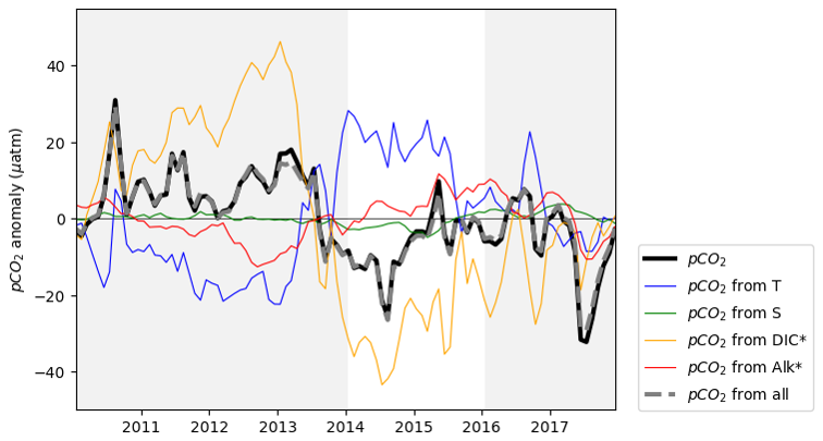
Figure 6 Time series of the contributions to oceanic pCO₂ anomaly referenced to 2010–2017 from SST (blue), SSS (green), DIC^* (yellow), ALK^* (red), and the combined effect of all variables (grey dashed) at OSP. The black line is the oceanic pCO₂ directly output from the model. All variables are detrended and deseasonalized. The unshaded period corresponds to 2014–2015, during which the Blob occurred. The grey dash line is the sum of individual components that closely matches the total pCO₂, supporting the linearity of Eq. (1).

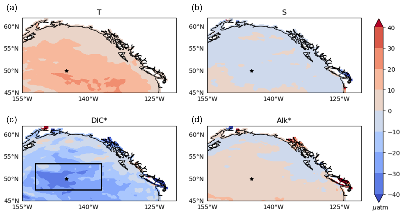
Figure 7 Spatial patterns of the contributions to oceanic pCO₂ from (a) SST, (b) SSS, (c) DIC^*, and (d) ALK^* during 2014–2015. Blue shows CO₂ uptake, and red shows CO₂ outgassing. The star in each panel marks the location of OSP. The black box (47.5–53.5° N, 208–223° E) in (c) indicates the central GOA area used for the budget analysis shown in Figs. 8 and 9.

The decrease in DIC during the Blob happened not only at OSP but throughout the whole central GOA. Figure 7 showed the spatial distributions of the oceanic pCO₂ changes calculated from the model outputs of each variable, same as in Fig. 6 during the Blob. The characteristic described above, namely, the mutual compensation between the SST and DIC, also holded in the entire region. These two factors counteracted each other, resulting in a relatively small decrease in oceanic pCO₂ due to the larger decrease in DIC. The magnitude of the oceanic pCO₂ declined peaks in the central GOA around the location of OSP.

3.4 Simulated DIC mass balance

To investigate the factors causing the significant decrease in DIC during the Blob, the surface ocean DIC mass balance was examined by the diagnosis of the DIC tendency terms. In the simplest form, the DIC mass balance was explained by three components: physical transport, biological activity, and air–sea gas exchange.

$$\begin{array}{}\text{(2)}& \begin{array}{rl}{\displaystyle \frac{\mathrm{d}C}{\mathrm{d}t}}& =\left(\mathrm{transport}\right)+\left(\text{biological activity}\right)\\ & +\left(\text{air-sea gas transfer}\right)\end{array}\end{array}$$

On the right-hand side of Eq. (2), the transport term included resolved advective transport convergence and parameterized mixing terms. Zonal, meridional and vertical advection of DIC, parameterized mixing, as well as the total transport convergence were calculated online and recorded as daily means. Biological activity included the net effects of photosynthetic carbon fixation, phytoplankton mortality, remineralization of dissolved and particulate organic matter, and the production and dissolution of calcium carbonates. These carbon tendency terms ($\frac{\mathrm{d}C}{\mathrm{d}t}$) were calculated for each timesteps and were recorded as daily averages. The tendency terms calculated at OSP were integrated over the 24 km radius centred at OSP. To put OSP into context within the larger region (central GOA), rates were calculated within 47.5–53.5° N, 208–223° E, shown with a black box in Fig. 7c. In both cases, the tendencies were integrated from the surface to 177.5 m, with units of molC s⁻¹. This depth range was greater than the maximum mixed layer depth diagnosed in our simulation and thus guarantees that vertical integration contained the entire mixed layer regardless of seasonal variability.

Figure 8 showed the time series of each carbon tendency component at OSP (within 24 km radius) and in the central GOA (box in Fig. 7c), after removing the linear trend and mean seasonal cycle and applying a 30 d moving window average. First, the sum of these three tendency components (Eq. 2) exactly matched the DIC tendency (i.e. left-hand side of Eq. 2). The variability of DIC was almost completely explained by the transport term throughout the entire period, while the effects of the other two components were relatively minor. At OSP, an extremely negative anomaly in DIC transport convergence rapidly developed in the winter of 2013, coinciding with the onset of the Blob. This anomaly was unprecedented compared to other periods. In the central GOA, a negative DIC transport anomaly appeared slightly earlier, in early 2013, and, as at OSP, intensified again in the winter of 2013. These anomalies led to a pronounced DIC decrease at the onset of the Blob, driven by changes in physical transport processes.

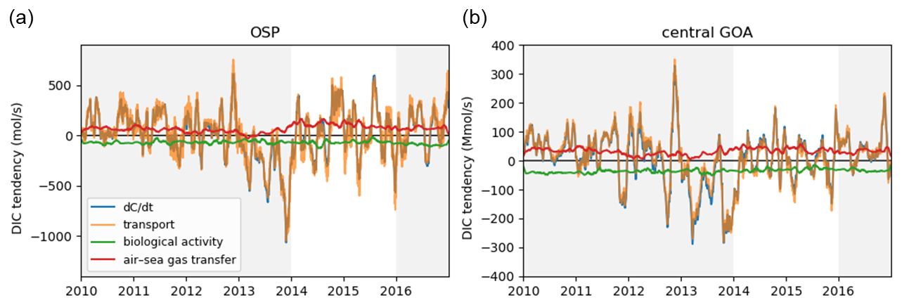
Figure 8 Time series of vertically integrated DIC tendencies from the surface to 177.5 m at (a) OSP and (b) the central GOA which is defined in Fig. 7c. The time derivative of DIC is shown in blue; changes in DIC due to transport are shown in orange, due to biological activity in green, and due to air–sea gas transfer in red. All variables are detrended, deseasonalized, and smoothed using a 30 d moving average. The unshaded period corresponds to 2014–2015, during which the Blob occurred.

Among the physical processes responsible for the DIC reduction during the Blob, the vertical transport dominated over the large-scale domain, whereas locally the effects of the horizontal transport were comparable to those of the vertical transport. To better understand the transport-driven DIC changes, the transport term can be decomposed into individual components (horizontal and vertical advection) and the parameterized turbulent mixing terms. The background physical transport of DIC in the GOA was governed by both vertical and horizontal advection processes. Upwelling supplied DIC-enriched subsurface waters to the surface, while the prevailing westerlies drived a southward Ekman transport of DIC-rich surface waters from the northern part of the domain, where surface DIC concentrations were higher, to the southern part of the domain (Fig. S1a).

Figure 9 showed the time series of each advective component of DIC tendency at OSP and in the central GOA. In the central GOA, the transport-driven DIC changes were primarily controlled by the vertical transport. This was because the small-scale horizontal transport within the computational domain was averaged out, and the transport across the domain boundaries can only play secondary roles in the regional DIC budget. Focusing on the DIC decrease in the winter of 2013, a pronounced DIC reduction associated with decreased vertical transport was evident, indicating suppressed upward transport of DIC-rich waters from the ocean interior to the surface layer due to enhanced stratification caused by elevated water temperatures.

At OSP, the effect of the horizontal transport was more important locally relative to the larger domain in the central GOA. Changes in DIC reflected the combined contributions of the vertical and horizontal transport, and their relative contributions were quantified. In the winter of 2013, the net contribution of the horizontal transport accounted for approximately half of the total DIC decrease (−531.0 molC s⁻¹), while the remaining half was attributable to a reduction in the vertical transport (−533.7 molC s⁻¹). This DIC decrease associated with horizontal transport resulted from strengthened south-easterly currents in the winter of 2013. As shown in Fig. S3, anomalous south-easterly currents intensified from autumn to winter 2013, reducing the southward transport of DIC-rich surface waters that was typically supplied by Ekman transport from the north. However, as noted above, such south-easterly flow anomalies were not clearly evident over the entire model domain. Figure S3 also shows a clear shift toward negative DIC anomalies from 2013 to 2014. Consequently, the local DIC reduction at OSP during the Blob was driven by two mechanisms: anomalous south-to-north transport of low-DIC waters and suppressed upward transport of DIC-rich subsurface waters. These transport anomalies were consistent with the reduced Ekman transport associated with the weakened Aleutian Low that generated the anomalously high sea level pressure and SST (Bond et al., 2015; Hartmann et al., 2015).

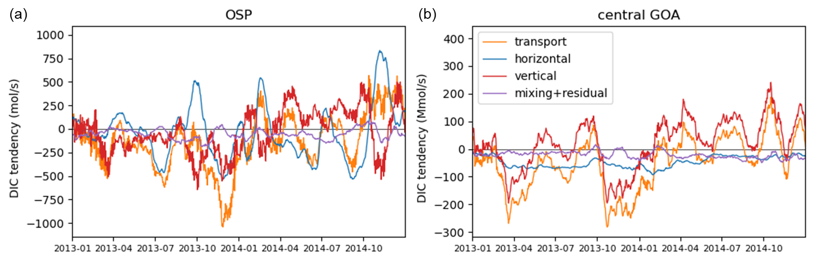
Figure 9 Time series of vertically integrated DIC tendencies from the surface to 177.5 m at (a) OSP and (b) the central GOA, which is defined in Fig. 7c, for each transport component: horizontal advection (blue), vertical advection (red), and the mixing and residual term (purple), calculated as the remainder after subtracting the advective components from the total transport (orange). All variables are detrended, deseasonalized, and smoothed using a 30 d moving average. The unshaded period corresponds to 2014–2015, during which the Blob occurred.

3.5 Drivers of the simulated weakening of physical transport

The reduction in vertical DIC transport in the central GOA was driven by two key mechanisms: enhanced stratification associated with SST warming and weakened Ekman pumping caused by reduced wind-driven circulation. Compared with the DJF climatology, potential density in the winter 2013 exhibited substantially lower between 160° W and 140° W (Fig. 10), indicating strengthened stratification that suppressed the upward transport of DIC-rich subsurface waters and reduced the DIC supply to the surface.

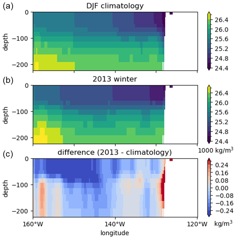
Figure 10 Vertical cross-sections of potential density along 50.5° N for (a) the DJF-mean climatology over 2010–2017, (b) 2013, and (c) their difference (2013 minus climatology).

In addition, although the GOA was typically characterized by Ekman upwelling, the period immediately preceding the onset of the Blob was marked by weakened wind stress curl and Ekman downwelling (Fig. 11), further suppressing the vertical DIC supply. These potential density and wind stress curl changes were fully consistent with both the marine heatwave itself and the weakening of the Aleutian Low that initiated the Blob. Together, these early-stage changes reduced surface DIC and exerted a substantial influence on oceanic pCO₂ throughout the Blob period. This highlights the critical role of early physical forcing in shaping the prolonged carbon cycle response during the Blob.

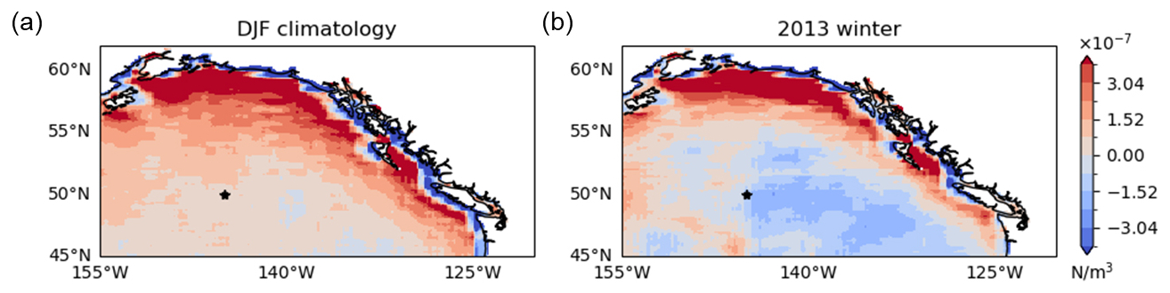
Figure 11 Spatial patterns of wind stress curl (curl τ) for (a) the DJF-mean climatology over 2010–2017 and (b) 2013. Positive values indicate cyclonic flow associated with Ekman upwelling. The star in each panel marks the location of OSP.

4 Discussion

Both the model and the SeaFlux product showed enhanced oceanic CO₂ uptake during the Blob. This increase was primarily driven by changes in surface ocean pCO₂. Here, CO₂ flux was treated as a complementary diagnostic of the integrated air–sea CO₂ response to the Blob, given its nonlinear dependence on wind speed, temperature, and ΔpCO₂. The spatial distribution of the CO₂ flux indicated net oceanic CO₂ uptake over most of the GOA domain, while enhanced outgassing (ocean to atmosphere), which was not evident in SeaFlux ensemble mean, was simulated in the northwestern region (Fig. S4), consistent with the elevated oceanic pCO₂ in this area (Figs. 2 and 3). This positive bias in the northwestern GOA was also reflected in other variables.

In the area-integrated CO₂ flux time series for the central GOA (Fig. S5), the model exhibited weaker uptake than the SeaFlux ensemble mean during all periods, with values of −8.2 Tg yr⁻¹ versus −10.9 Tg yr⁻¹ before the Blob (2010–2013), −13.4 Tg yr⁻¹ versus −19.0 Tg yr⁻¹ during the Blob (2014–2015), and −12.9 Tg yr⁻¹ versus −14.8 Tg yr⁻¹ after the Blob (2017), respectively (the model versus the SeaFlux ensemble mean). Given that both products use JRA55 winds and that differences in CO₂ solubility are negligible, this discrepancy likely arised from differences in ΔpCO₂ and/or the gas transfer coefficient. Both the model and the SeaFlux ensemble showed overall good agreement with the mooring observations (Fig. 5), although the degree of agreement varies by year. Therefore, the weaker modeled CO₂ uptake did not necessarily imply reduced model fidelity.

Our results showed that the reduction in DIC during the Blob was primarily driven by physical processes such as Ekman transport and vertical entrainment. Beyond the oceanic pCO₂ changes, numerous biological impacts of MHWs have also been reported. These include observed declines in annual net community production (Yang et al., 2018), reductions and taxonomic shifts in phytoplankton biomass, transitions in plankton communities from larger to smaller taxa (Du and Peterson, 2018; Peña et al., 2018; Batten et al., 2022). Whether ecosystem impacts can return to pre-MHW conditions remains uncertain (Suryan et al., 2021). The magnitude and nature of these biological responses vary greatly among regions, and a key factor is whether the area is primarily limited by nitrate or iron to the biological production (Peña et al., 2018; Hayashida et al., 2020; Wyatt et al., 2022). Because the GOA is an iron-limited region, it is likely less sensitive to MHW-induced macro-nutrient reductions than regions farther south in the subtropics and the transition zone (30–45° N, Wyatt et al., 2022). Nevertheless, model-based analyses will be essential for assessing long-term and basin-scale impacts. The biogeochemical model used in this study is relatively simple, and it does not explicitly represent shifts in plankton community composition. Revisiting this problem with a more sophisticated ecosystem model would be warranted to assess such ecological changes and determine their duration and magnitude.

Compared to the study conducted over broader spatial domains (Mignot et al., 2022), our results revealed a distinct response of oceanic pCO₂ to MHWs in the GOA. This highlights the importance of investigating the impacts of MHWs on oceanic pCO₂ in other regions as well. For instance, persistent positive SST anomalies have also been reported in the western North Pacific, particularly in the Oyashio region (40–43° N and 143–147° E, Miyama et al., 2021), which is one of the major carbon uptake areas in the basin. However, it remains unclear how oceanic pCO₂ in this region responded to such anomalies. It is important to expand the model domain to a broader area including the western North Pacific.

Abnormally high ocean temperatures like the Blob have been increasing in both frequency and duration (Frölicher et al., 2018; Oliver et al., 2018). The North Pacific experienced anomalously high SSTs in other years such as 2019 (Amaya et al., 2020) and 2023 (Dong et al., 2025). These MHWs exhibit even larger SST anomalies than the Blob and differ in several key characteristics, such as the timing of the peak warming (Amaya et al., 2020). Consequently, their impacts on oceanic pCO₂, carbon cycling, and marine ecosystems may differ from those during the Blob. Indeed, the 2023 MHW showed a markedly different behaviour on a global scale, with an approximately 10 % reduction in oceanic CO₂ uptake, substantially larger than in previous events (Müller et al., 2025). These contrasts call for event-specific investigations of individual MHWs. In this context, a similar analysis of the 2005 warm anomaly event in the GOA showed qualitatively comparable results to the Blob, in that the DIC decrease and associated reduction in oceanic pCO₂ were primarily controlled by changes in vertical transport. Although not shown, these results suggest that the proposed mechanism may operate under certain warm anomaly conditions in the GOA. However, its applicability is not necessarily universal and may depend on the characteristics and intensity of individual events, particularly for recent stronger MHWs.

The model employed in this study was integrated only through 2017 due to the availability of the open boundary conditions. Future work should extend the integration period, for instance by applying alternative boundary conditions, to assess the impacts of the 2019 and 2023 MHWs on oceanic pCO₂.

5 Conclusions

From the winter of 2013 to 2015, the eastern North Pacific experienced an anomalously high in SST. Contrary to expectations based on the reduced CO₂ solubility under warming, oceanic pCO₂ did not rise. Instead, it decreased across the entire region, with a particularly large decrease in the open ocean (Figs. 2 and 3). To investigate why oceanic pCO₂ broadly decreased during the Blob, the simulation results from the regional ocean circulation and biogeochemistry model were analyzed. The model represents the oceanic pCO₂ remarkably well compared to the observations (Figs. 4 and 5). The decomposition of the oceanic pCO₂ anomalies into four components shows that the variability in the oceanic pCO₂ is primarily dominated by changes in SST and DIC. Furthermore, the effects of these two factors generally compensate for one another. During the Blob, the reduction in oceanic pCO₂ due to a decrease in DIC was stronger in magnitude than the warming-induced increase (Figs. 6 and 7). The pronounced reduction in DIC under the Blob is attributable not to biological processes, but rather to the anomalous physical transport (Fig. 8). In particular, reduced vertical DIC transport in the central GOA, driven by enhanced stratification and weakened Ekman pumping, was the primary mechanism (Figs. 9–11). Consequently, these changes in the vertical circulation decreased the surface DIC concentrations, leading to a subsequent decline in the oceanic pCO₂ during the Blob.