Revealing hidden oxygen variability in the North Pacific: a two-decade analysis using GOBAI-O₂

Oceanic dissolved oxygen concentrations are thought to be declining under ongoing global warming, yet their variability remains less well understood than that of physical parameters such as temperature and salinity, primarily due to the limited spatial and temporal coverage of oxygen observation. Here, we examine linear trends in potential temperature, salinity, and dissolved oxygen in the North Pacific over the past two decades (2004–2023), using the GOBAI-O₂-v2.2 dataset (Version 4.4). We compare the diagnosed oxygen trends with those of physical parameters to reveal the spatial structure of recent changes. The oxygen trends inferred from GOBAI-O₂ are broadly consistent with trends observed along ship-based hydrographic repeat lines. While basin-scale deoxygenation is evident, we also identify localized oxygen increases on specific density surfaces. By relating these patterns to the surrounding physical environment, we find that the spatial heterogeneity in oxygen trends is consistent with known oceanographic processes, including the southward retreat of the oxygen minimum layer and the northward migration of a front separating the subtropical and subarctic gyres. These results underscore the value of GOBAI-O₂ data in linking physical variability to previously unrecognized biological and biogeochemical patterns in the ocean.

1 Introduction

Over recent decades, the global ocean has experienced a decline in its dissolved oxygen inventory, a trend projected to continue through the 21st century (Keeling et al., 2010; Breitburg et al., 2018; Stramma and Schmidtko, 2021; Limburg et al., 2020; Ito et al., 2017, 2024; Kolodziejczyk et al., 2024). This deoxygenation is driven in part by reduced ocean oxygen solubility under rising sea-surface temperatures, which promotes oxygen outgassing. In addition, enhanced stratification and a slowdown of ocean circulation under global warming can reduce interior ventilation and oxygen supply (Keeling et al., 2010; Bopp et al., 2013; Ito et al., 2017). Ocean oxygen loss can negatively affect aerobic marine organisms (Pörtner and Farrell, 2008; Sampaio et al., 2021), alter biogeochemical cycles, and potentially induce climate-relevant feedback (Berman-Frank et al., 2008). Historical deoxygenation has been inferred from globally distributed observations (Helm et al., 2011; Schmidtko et al., 2017; Ito et al., 2017; Takatani et al., 2012; Sasano et al., 2015; Lauvset et al., 2022), and Earth system models have been used to simulate both historical and future changes in ocean oxygen (Bopp et al., 2013; Kwiatkowski et al., 2020; Li et al., 2020).

Observed oxygen trends have traditionally been assessed using the discrete measurements of dissolved oxygen concentration (O₂), typically obtained by Winkler titration (Winkler, 1888). These measurements are also used to calibrate electrode- and, more recently, optode-based oxygen sensors mounted on conductivity-temperature-depth (CTD) profilers (Helm et al., 2011; Schmidtko et al., 2017; Lauvset et al., 2022). Although programs such as WOCE, CLIVAR, and GO-SHIP have collected high-quality oxygen measurements globally, repeat occupation intervals are commonly on the order of a decade, limiting the ability to robustly quantify annual to seasonal variability. Higher-frequency ship-based observations exist in a few regions (Takatani et al., 2012; Sasano et al., 2015), but their spatial coverage is limited. Consequently, despite attempts to characterize basin-scale patterns (Ito et al., 2017; Stramma et al., 2020; Kolodziejczyk et al., 2024), observational constraints have hampered a spatially and temporally comprehensive understanding of dissolved oxygen variability and trends.

Oxygen sensors were first deployed on Argo profiling floats in the mid-2000s. Since then, approximately 1800 oxygen-equipped floats have been deployed worldwide, substantially advancing the observational basis for assessing oxygen variability and trends (Sharp et al., 2023). The expansion toward a global biogeochemical (BGC) Argo network has improved sampling in regions that were previously sparsely observed (Claustre et al., 2020). In parallel, major progress has been made in calibration, adjustments, and quality control of oxygen measurements, including pre-deployment drift corrections (D'Asaro and McNeil, 2013; Johnson et al., 2015; Bittig and Körtzinger, 2015; Bushinsky et al., 2016; Drucker and Riser, 2016; Nicholson and Feen, 2017), climatology-based calibrations (Takeshita et al., 2013), in-air oxygen measurement calibrations (Körtzinger et al., 2005; Bittig and Körtzinger, 2015; Johnson et al., 2015; Bushinsky et al., 2016), post-deployment drift corrections (Johnson et al., 2017; Bittig et al., 2018a, b), and the standardized delayed-mode quality control procedures (Maurer et al., 2021). Together, these developments have reduced uncertainty and improved the consistency of optode-based [O₂] measurements from Argo floats.

To date, oxygen observations from Argo floats have been used primarily in regional process studies, including air-sea oxygen exchange (Wolf et al., 2018), upper-ocean primary production (Alkire et al., 2012; Estapa et al., 2019), biological pump efficiency (Johnson and Bif, 2021), and the dynamics of the oxygen minimum zone (Udaya Bhaskar et al., 2021). Recently, Sharp et al. (2023) produced a four-dimensional gridded [O₂] product, GOBAI-O₂ (Gridded Ocean Biogeochemistry from Artificial Intelligence (AI) – Oxygen). GOBAI-O₂ is constructed using machine-learning methods trained on oxygen observations and designed to reconstruct spatial patterns, seasonal cycles, and decadal variability, particularly in regions where observational data gaps coincide with high background O₂ variability.

In the North Pacific, several studies have documented heterogeneous oxygen trends. Using an objectively mapped monthly climatology of O₂ based on the World Ocean Database 2013 (WOD13) (Boyer et al., 2013), Ito et al. (2017) reported multidecadal variability and trends in dissolved O₂ in the surface-layer oxygen from 1958 to 2013. Sasano et al. (2015), using the high-frequency shipboard sections along the 137 and 165° E lines from 1987 to 2011, reported oxygen declines in the northern subtropical to subtropical-subarctic transition zones of $-\mathrm{0.45}\pm \mathrm{0.16}$ µmol kg⁻¹ yr⁻¹ at 25.3 σ_θ and $-\mathrm{0.45}\pm \mathrm{0.14}$ µmol kg⁻¹ yr⁻¹ at 26.8 σ_θ, respectively. They also identified a significant oxygen increase in the tropical Oxygen Minimum Layer (OML) of $+\mathrm{0.36}\pm \mathrm{0.004}$ µmol kg⁻¹ yr⁻¹, highlighting pronounced spatial heterogeneity in oxygen trends. At broader scales, Stramma et al. (2020) analyzed historical bottle data and reported links between oxygen variability and climate modes such as the Pacific Decadal Oscillation (PDO) and the North Pacific Gyre Oscillation (NPGO), although sparse sampling makes it difficult to robustly connect regional trends to physical mechanisms. Collectively, previous studies indicate that oxygen changes in the North Pacific can be strong, spatially non-uniform, and potentially driven by both circulation/ventilation changes and biologically mediated oxygen consumption (Sasano et al., 2015, 2018; Ito et al., 2017; 2024; Stramma et al., 2020; Kolodziejczyk et al., 2024).

Because observational opportunities to quantify trends in dissolved oxygen – together with concomitant changes in temperature and salinity – remain limited, gridded products such as GOBAI-O₂ are becoming increasingly valuable for basin-scale analyses. In this study, we use GOBAI-O₂ to quantify linear trends in potential temperature, salinity, and dissolved oxygen in the North Pacific over 2004–2023 and examine how their trends are connected in both depth and density space. We further discuss the extent to which the diagnosed oxygen trends can be interpreted in terms of physical drivers, including surface warming, stratification changes, and circulation variability in the North Pacific.

2 Data and Methods

2.1 GOBAI-O₂ dataset

We use GOBAI-O₂-v2.2 (Version 4.4), a four-dimensional, monthly gridded product of dissolved oxygen (O₂) in the ocean interior, generated using machine learning (ML) algorithms trained on both Argo float oxygen measurements and ship-based discrete observations (Sharp et al., 2023). GOBAI-O₂ is mapped onto the temperature-salinity fields provided by the global Argo array (Roemmich and Gilson, 2009). The underlying oxygen training database combines ship-based measurements from GLODAPv2.2022 and Argo float data distributed through the Argo Global Data Assembly Centers, after quality control (Sharp et al., 2022, https://doi.org/10.25921/z72m-yz67).

According to Sharp et al. (2023), the float data used in GOBAI-O₂ were filtered to retain only delayed-mode adjusted profiles with quality flags of 1 (good), 2 (probably good), or 8 (interpolated/extrapolated) for pressure, temperature, salinity, and dissolved oxygen. Among all available float profiles, 51.4 % underwent quality control through comparison with climatological fields from the World Ocean Atlas (WOA) or the Commonwealth Scientific and Industrial Research Organisation Regional Sea Atlas (CARS). An additional 30.3 % were evaluated using atmospheric oxygen concentration measurements, and 7.0 % were quality controlled through comparison with in-water measurements (WOD, OMS assuming an oxygen zero, or deployment-time CTD profiles). A further 5.3 % were adjusted using in-situ optode calibration based on the method of Drucker and Riser (2016), 3.3 % were adjusted by other methods, 1.9 % were unclassified, and the remaining 0.9 % were not adjusted.

The ML models predict O₂ using predictors that include absolute salinity, conservative temperature, potential density anomaly, hydrostatic pressure, bottom depth, and additional spatiotemporal covariates representing geographic, seasonal, and interannual variability. Biological processes are not explicitly parameterized in the ML framework; however spatiotemporal covariates can implicitly capture biological influences to some extent (Giglio et al., 2018).

GOBAI-O₂ is produced using two ML approaches: feed-forward networks (FNNs) and random forest regression (RFRs, (Breiman, 2001)). The final O₂ estimate at each grid point is taken as the mean of the FNN and RFR predictions. The dataset spans 2004–2023 at monthly resolution on a 1° × 1° latitude–longitude grid, covering 86 % of the global ocean area. The product is provided on 58 vertical levels from the surface to ∼2000 m. Sharp et al. (2023) reported 0.79±0.04 % per decade decrease in the oxygen inventory of the upper 2000 m over 2004–2022. Full details of their data sources, processing, algorithm training, evaluation, and uncertainty estimation are given in Sharp et al. (2023).

2.2 Uncertainty estimates

GOBAI-O₂ provides an uncertainty estimate for each gridded O₂ value, constructed by combining independent uncertainty components in quadrature (Sharp et al., 2023):

$$\begin{array}{}\text{(1)}& u(\left[{\mathrm{O}}_{\mathrm{2}}\right]{)}_{\mathrm{tot}.}=\sqrt{u(\left[{\mathrm{O}}_{\mathrm{2}}\right]{)}_{\mathrm{meas}.}^{\mathrm{2}}+u(\left[{\mathrm{O}}_{\mathrm{2}}\right]{)}_{\mathrm{grid}.}^{\mathrm{2}}+u(\left[{\mathrm{O}}_{\mathrm{2}}\right]{)}_{\mathrm{alg}.}^{\mathrm{2}}},\end{array}$$

where $u\left(\right[{\mathrm{O}}_{\mathrm{2}}]{)}_{\mathrm{meas}.}^{\mathrm{2}}$ represents measurement uncertainty of the underlying observations, $u\left(\right[{\mathrm{O}}_{\mathrm{2}}\left]{)}_{\mathrm{grid}.}^{\mathrm{2}}\right)$ is the gridding uncertainty associated with representing a four-dimensional spatiotemporal volume by a single value, and $u\left(\right[{\mathrm{O}}_{\mathrm{2}}]{)}_{\mathrm{alg}.}^{\mathrm{2}}$ is the algorithmic uncertainty arising from the ML estimation. We use u([O₂])_tot. to characterize uncertainty in O₂ and to propagate uncertainty into our oxygen trend estimates (Figs. 1–4). In most figures, we incorporate the mean uncertainty when estimating linear O₂ trends.

2.3 Vertical grid and interpolation for isopycnal analysis

GOBAI-O₂ is provided on a 1° × 1° horizontal grid with 58 depth levels: 2.5, 10, 30, 40, 50, 60, 70, 80, 90, 100, 110, 120, 130, 140, 150, 160, 170, 182.5, 200, 220, 240, 260, 280, 300, 320, 340, 360, 380, 400, 420, 440, 462.5, 500, 550, 600, 650, 700, 750, 800, 850, 900, 950, 1000, 1050, 1100, 1150, 1200, 1250, 1300, 1350, 1412.5, 1500, 1600, 1700, 1800, 1900 and 1975 m. The enhanced near-surface vertical resolution is important for resolving strong gradients in temperature, salinity, density, and oxygen within the mixed layer (Kara et al., 2000).

For analysis performed in density space, we interpolate the original depth-level data to 1 m vertical grid using cubic spline interpolation and then evaluate linear trends on a 1° × 1° × 1 m grid. This approach enables computation of trends as a function of latitude (1° bins) and potential density anomaly (0.1 σ_θ bins) (Figs. 4–7). To evaluate sensitivity to interpolation choices, we repeated the analysis using linear, shape-preserving cubic (PCHIP) interpolation and using coarser vertical grids (2 and 5 m). The resulting trend patterns show no material differences among interpolation methods (Figs. S1a, b and S2a, b in the Supplement). The 5 m grid cannot resolve densities lighter than 24.0 σ_θ at some latitudes; however, the main features are preserved across all tested resolutions.

2.4 OFES model output

In Sect. 3.3.2, we additionally use output from the eddy-resolving OGCM for the Earth Simulator (OFES) (Masumoto et al., 2004; Masumoto, 2010; Sasaki et al., 2008) to examine the physical context of the diagnosed variability. OFES is based on the MOM3 (Pacanowski and Griffies, 2000) and uses a quasi-global domain spanning 75° S–75° N with 0.1° × 0.1° horizontal resolution and 54 vertical levels. The model was initialized from rest using the World Ocean Atlas 1998 (WOA98) (Boyer and Levitus, 1997), and spun up for 50 years using climatological forcing derived from NCEP-NCAR reanalysis (Kalnay et al., 1996). After spin-up, a hindcast experiment was conducted from 1950 to 2024 using daily NCEP-NCAR forcing. Here we analyze OFES output over 1950–2023.

2.5 GODAS model output

In Sect. 3.3.2, we also use temperature and salinity fields from the NCEP Global Ocean Data Assimilation System (GODAS) to complement our analysis. GODAS is a global ocean reanalysis system developed at the National Centers for Environmental Prediction (NCEP) and is based on the Modular Ocean Model version 3 (Pacanowski and Griffies, 2000). The system assimilates surface temperature profiles, XBT data, moored buoy observations, and other in situ measurements using a three-dimensional variational (3DVAR) assimilation scheme (Behringer and Xue, 2004; Behringer, 2007). The GODAS reanalysis is provided on a 1° × 1° horizontal grid with enhanced meridional resolution ($\mathrm{1}/\mathrm{3}$°) near the equator and includes 40 vertical levels. The reanalysis spans from 1980 to the present and is widely used for climate diagnostics and ocean variability studies. In this study, we analyze GODAS density fields over the period 2003–2024 by using temperature and salinity.

3 Results

3.1 Horizontal distributions of linear trends

Figure 1 illustrates the horizontal and vertical distributions of linear trends in potential temperature, salinity, and dissolved oxygen (O₂), over 2004–2023. Positive trends in potential temperature are primarily confined to the surface layer above 200 m depth (Fig. 1a–c), with larger magnitudes at higher latitudes. In contrast, negative trends emerge below the surface in the eastern tropical area (180–120° W, 5–15° N) (Fig. 1b), extending westward and deepening with increasing depth (Fig. 1d–f). Below ∼400 m, the spatial distributions of positive and negative temperature trends differ between the subarctic and subtropical gyres.

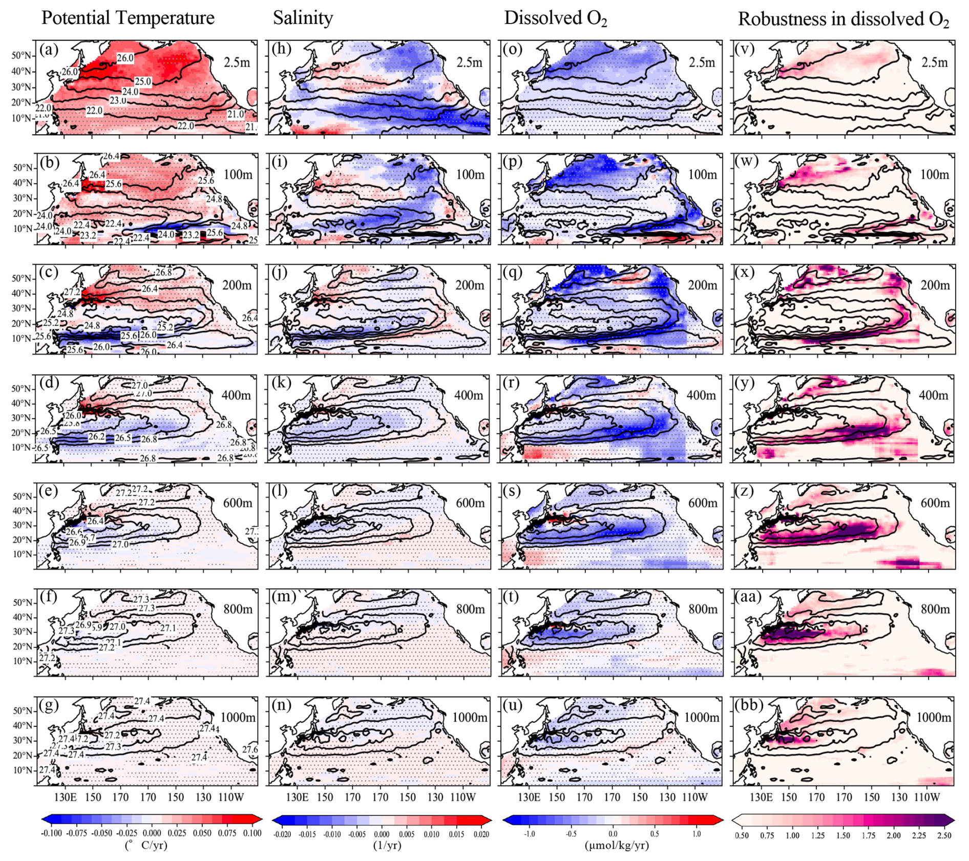
Figure 1 Horizontal distributions of linear trends in potential temperature (a–g), salinity (h–n), and dissolved oxygen (O₂) (o–u) during the observational period at depths of 0, 100, 200, 400, 600, 800, and 1000 m, respectively. Hatched areas indicate statistically significant trends at the 95 % confidence level based on a Student's t-test with effective degrees of freedom accounting for temporal autocorrelation. Trend significance was evaluated using a Student's t-test with effective degrees of freedom accounting for lag-1 autocorrelation. Contours denote potential density at each depth. Labels for the potential density are shown only in the potential temperature sections. Corresponding distributions of the Robustness (R), defined as the ratio of the trend magnitude to the dataset uncertainty in dissolved O₂ are presented in panels (v)–(bb).

Salinity trends exhibit generally negative values throughout the surface layer (Fig. 1h–i), consistent with freshening. Localized positive salinity trends are detected in the Kuroshio–Oyashio transition area and the northwest Pacific (140–180° E, 20–50° N), as well as in the tropical region (120–170° E, 0–10° N). Additional positive trends are observed along the eastern boundary off California (130–199° W, 20–40° N). Below 200 m depth, salinity trends are weaker and broadly mirror the temperature (Fig. 1j–k). Notably, negative salinity trends are evident around the Alaska gyre (170–130° W, 40–55° N) (Fig. 1j–l), a pattern that differs from the corresponding temperature trends.

Negative trends in dissolved O₂ are widespread across the North Pacific and extend throughout much of the water column (Fig. 1o–u). Large negative trends are concentrated at higher latitudes near the surface, with their locations shifting systematically with depth. Particularly strong O₂ declines are observed along the northeastern boundary (140–130° W, 40–50° N) and within the southern subtropical region (10–25° N) on density surfaces between 25.2 and 26.8 σ_θ, corresponding to depths of approximately 200–600 m (Fig. 1q–s). In contrast, weak positive O₂ trends are detected below 200 m depth in the Kuroshio–Oyashio transition zone (130–150° E, 30–40° N), extending into deeper layers and spreading northeastward across the basin (Fig. 1r–u).

Positive O₂ trends are restricted to specific regions and depths: the tropical region at ∼100 m depth (Fig. 1p); the Alaska Gyre at 200–400 m depth (Fig. 1q–r); the western tropical region at 400–600 m depth (Fig. 1r–s); and the Kuroshio–Oyashio transition region at similar depths (Fig. 1r–s). When examined as a function of latitude, the magnitudes of negative O₂ trends do not depend monotonically on latitude alone. While surface-layer declines are strongest at high latitudes, the largest negative trends at intermediate depths (400–600 m) occur in the mid-latitude band (30–40° N). This depth-dependent latitudinal structure implies the importance of remote transports and the circulation-driven redistribution of oxygen, rather than purely local surface forcing. The underlying mechanisms are discussed further in Sect. 3.3.

The total uncertainty in dissolved O₂, u([O₂])_tot., exhibits pronounced regional structure (Fig. 2a–g). Uncertainty is largest in the North Pacific north of 50° N and decreases toward lower latitudes. Relatively high uncertainty values are also evident in the surface layer, and within regions of strong density gradients in the eastern tropical Pacific [150–120° W, 10–30° N] at depths of 100–200 m (Fig. 2b–c). In general, uncertainty peaks near 100 m depth and decreases with increasing depth (Figs. 2 and A14 in Sharp et al. (2023)). As shown by Sharp et al. (2023), regional variations in uncertainty are dominated by algorithmic uncertainty rather than measurement or gridding components (Eq. 1). Elevated algorithmic uncertainty in the northern Pacific above 50° N and along the western and eastern tropical margins below 20° N reflects sparse observational coverage in these regions (Fig. 1 in Sharp et al., 2023).

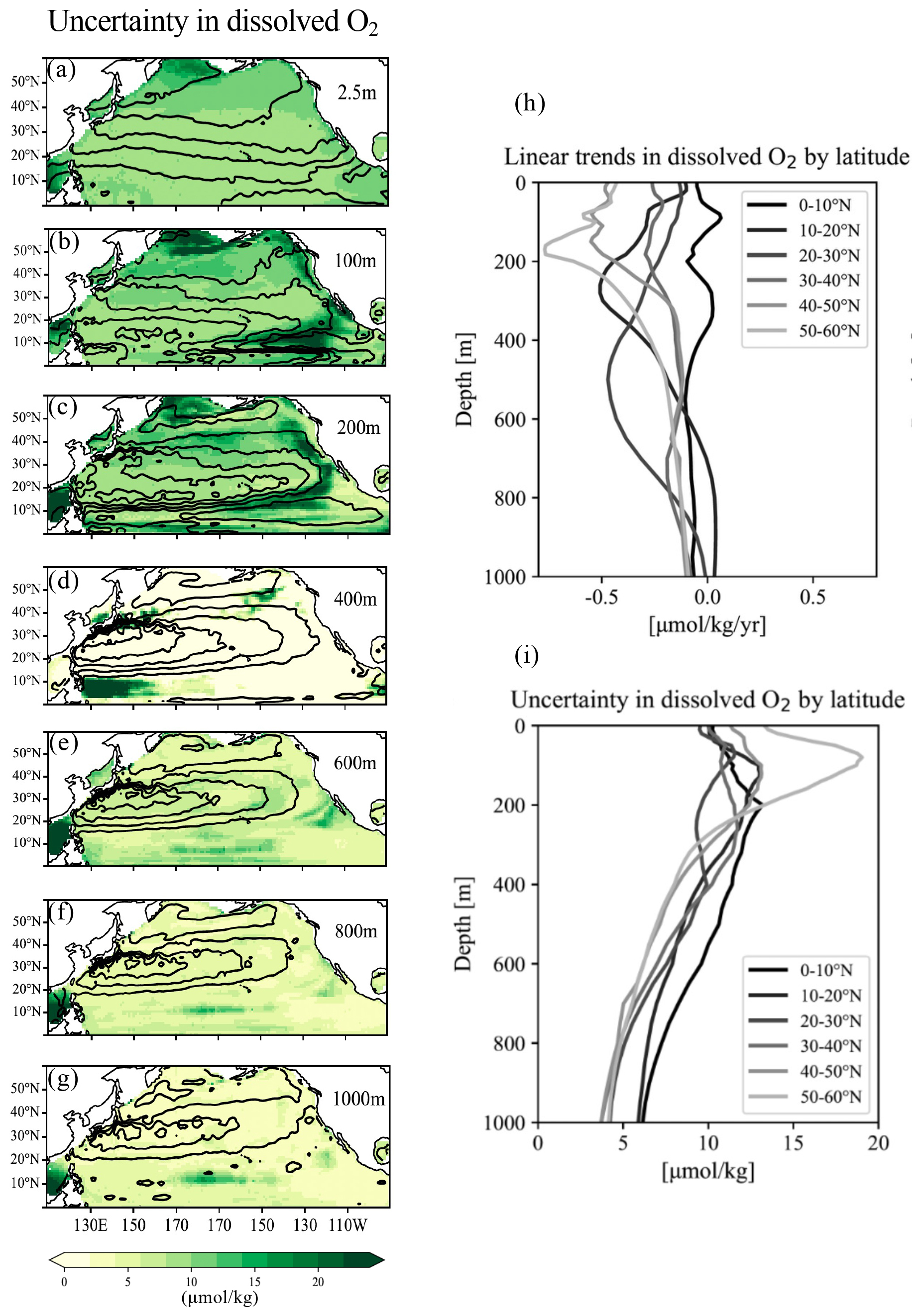
Figure 2 Horizontal distributions of dataset uncertainty in dissolved O₂ (a–g) and vertical profiles of linear trends and uncertainty in dissolved O₂ by latitude (h–i).

To assess whether regional trends exceed the dataset uncertainty, we computed the spatial distribution of Robustness (R), defined as $R=\left|\mathrm{trend}\mathrm{over}\mathrm{two}\mathrm{decades}\right|/\mathrm{uncertainty}$ (Fig. 1v–bb). (Note: This diagnostic provides a heuristic measure of the relative strength of the trend compared to the local uncertainty, rather than a formal quantification of uncertainty propagation.) The results indicate that R exceeds or approaches high values in the eastern and western tropical zones, the Kuroshio Extension region, portions of the subpolar North Pacific, and along the 27.2–27.4 σ_θ density surfaces at 800–1000 m depth. Based on this metric, larger oxygen trend magnitudes correspond to higher R values, more clearly distinguishable from the background uncertainty. Thus, in the upper ocean (2.5–100 m), trends are relatively robust in terms of the R metric, mainly in the northern North Pacific. At 200–400 m, robust signals appear both in the northern North Pacific and along the 25.2–26.0 σ_θ surfaces in the southern subtropical region, as well as in the eastern and western tropics. At 600–1000 m, the trends are robust within the subtropical gyre bounded by the 27.0 σ_θ surface.

Compared with the previously reported historical horizontal distributions of dissolved O₂ reported by Ito et al. (2017) (Fig. 3 in Ito et al., 2017), our analysis shows a broader spatial extent of negative trends across the North Pacific. Whereas data gaps increase with depth in Ito et al. (2017), the GOBAI-O₂ product provides more spatially continuous coverage, yielding distributions that are consistent with surrounding regions. In addition, positive O₂ trends detected here in the Kuroshio–Oyashio transition zone and the northeastern North Pacific on density surfaces of 26.8–27.0 σ_θ (Fig. 1r) were not clearly evident in the earlier O₂ anomaly analysis. Similarly, the positive trends identified in the western tropical Pacific below 400 m depth (Fig. 1r–t) are stronger and more spatially coherent than those reported previously.

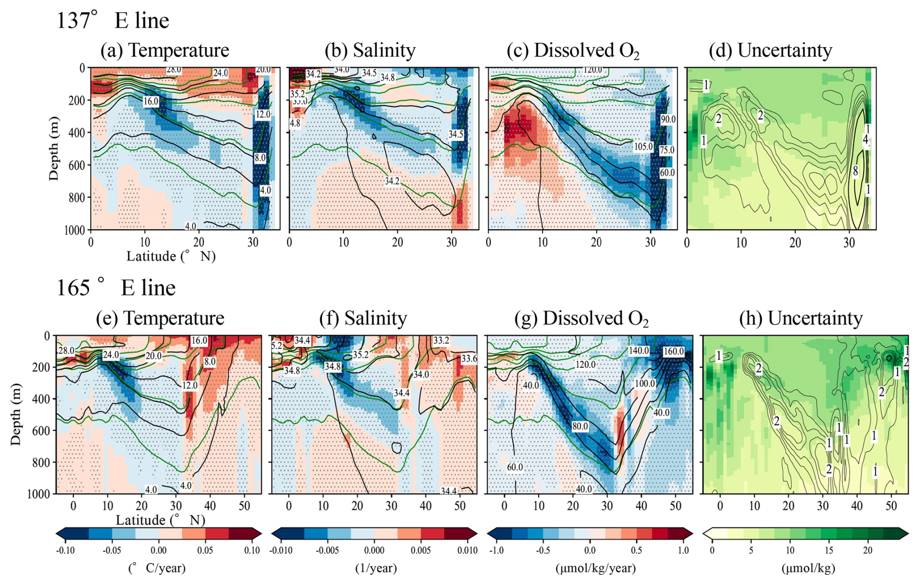
Figure 3 Vertical sections showing linear trends in potential temperature (a, e), salinity (b, f), and dissolved O₂ (c, g) along the 137 and 165° E meridians, respectively. Black contour lines indicate the mean potential temperature (a, f), salinity (b, g), and dissolved oxygen (c, h) over the period 2004–2023, while green contour lines represent the mean potential density. Labels for the potential density are shown only in the robustness sections. Hatched areas indicate statistically significant trends at the 95 % confidence level based on a Student's t-test with effective degrees of freedom accounting for temporal autocorrelation. Trend significance was evaluated using a t-test with effective degrees of freedom accounting for lag-1 autocorrelation. Corresponding vertical sections of the mean uncertainty with the contours of the Robustness (R) in panels (d) and (h). The contour intervals for thin and thick contours in (d) and (h) are 0.5 and 4.0, respectively.

The positive O₂ trends coincide with regions of relatively low uncertainty values (Fig. 1p–s and w–z), suggesting that they represent relatively robust features that are better constrained by the high observation density of Argo profiling floats. Other regions exhibiting positive signals – the northeastern North Pacific with a density range of 26.8–27.0 σ_θ (170° E–150° W, 45–55° N, Fig. 1r) and the tropical western Pacific (130–170° E, 0–10° N, Fig. 1r–t) – also correspond to areas of low uncertainty (Fig. 1y–aa). Consequently, these signals may reflect possible regional reoxygenation superimposed on the basin-scale deoxygenation trend.

Some localized expansions of the trend patterns, particularly in the tropical eastern Pacific (e.g. 170–130° W, 0–20° N) may partly reflect regions of elevated uncertainty, occasionally exceeding 15 µmol kg⁻¹ (Figs. 1q–s; 4i). Such large uncertainties would likely arise from sparse observations and high background variability (Sharp et al., 2023). Additional bias may stem from sensor calibration limitations in Argo oxygen measurements, especially in oxycline regions where finite optode response times can introduce systematic errors (Bittig et al., 2014, 2018a, b). Despite these caveats, the spatial patterns of the diagnosed O₂ trends are generally smooth and coherent across the basin. Based on statistical significance testing, most trends are significant throughout the water column (Fig. 1o–u). Overall, despite the uncertainties associated with the various factors discussed above, the GOBAI-O₂ dataset provides an improved framework for diagnosing basin-scale oxygen variability and its physical drivers.

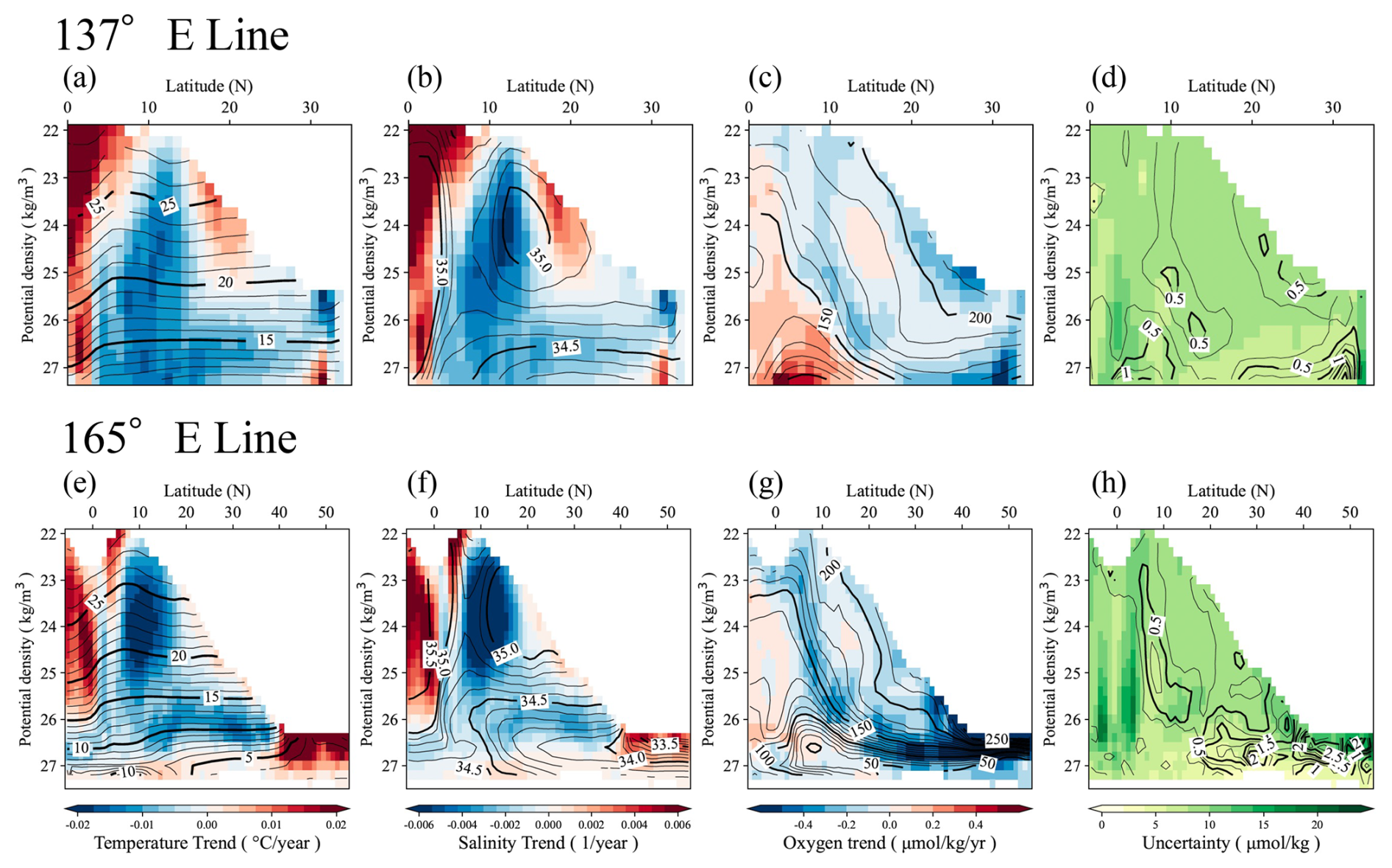
Figure 4 Linear trends in potential temperature (a, e), salinity (b, f), and dissolved O₂ (c, g) on each isopycnal surface at intervals of 0.1 σ_θ, calculated at every 1.0° of latitude in 137 and 165° E lines, respectively. Contour lines represent the mean values during the target observation periods, plotted at intervals of 0.1 σ_θ for each 1° of latitude. Panels (d) and (h) show the corresponding vertical sections of mean uncertainty, along with contours of robustness (R). The contour intervals for thin and thick contours in (d) and (h) are 0.25 and 0.5, respectively.

3.2 Vertical sections and isopyncal density analysis of linear trends in 137 and 165° E lines

To facilitate direct comparison with historical ship-based observations, we examine vertical sections and isopycnal distributions of linear trends in potential temperature, salinity, and dissolved O₂ along the 137 and 165° E meridional sections (Fig. 3). Ogata and Nonaka (2020) analyzed salinity data from 20 years of shipboard observations along the 137° E line between 1997 and 2016, while Sasano et al. (2015) analyzed temperature, salinity, and dissolved O₂ data from 25 years of cruises along the 165° E line between 1987 and 2011.

Along both sections, large negative trends in potential temperature and salinity are concentrated along the 25.0–26.0 σ_θ isopycnal surfaces, corresponding to potential temperatures of approximately 10–12° C and salinities of 34.4–34.5 (Fig. 3a, b, e, f). In contrast, the strongest negative trends in dissolved O₂ occur primarily along denser isopycnals between 26.0 and 27.0 σ_θ (Fig. 3c, g). This vertical separation indicates that the regions of pronounced oxygen decline are not co-located with those of temperature and salinity trends, implying distinct controlling mechanisms.

In addition to widespread oxygen declines, pronounced positive O₂ trends are detected south of ∼15° N below 200 m depth along the 137° E line (Fig. 3c). These positive trends are located near the upper boundary of the oxygen minimum layer (OML). Comparison with the corresponding uncertainty distributions (Fig. 3d, h) shows that regions exhibiting positive or negative oxygen trends generally do not coincide with areas of elevated uncertainty, indicating that these signals are robust within the GOBAI-O₂ framework.

The distributions of linear trends on isopycnal surfaces further highlight differences among temperatures, salinity, and dissolved O₂ (Fig. 4). Trends in temperature and salinity are closely aligned, with warming accompanied by salinification and cooling accompanied by freshening (Fig. 4a–b, d–e). In the tropical region (5° S–5° N), distinct positive trends in both variables are evident over the density range of 22.0–26.0 σ_θ. In contrast, little systematic trend is detected in the salinity minimum region (S = 34–34.1) within the density range of 26.5–27.0 σ_θ. At higher latitudes (40–50° N), strong positive trends in both temperature and salinity are observed along the 26.0–27.0 σ_θ surfaces (Fig. 4e).

Dissolved oxygen trends exhibit a markedly different structure. Although negative O₂ trends dominate overall, weak but coherent positive trends appear across the density range 23.0–26.0 σ_θ in low-latitude regions (5° S–5° N). More pronounced positive O₂ trends are detected in the deeper density range of 26.0–27.0 σ_θ between 5 and 10° N. Additional weak positive trends are observed between 10 and 20° N within the density range of 23.0–25.0 σ_θ along both the 137 and 165° E sections.

Compared with previous studies, the GOBAI-O₂-based trends reveal both similarities and notable differences. The general characteristics of temperature and salinity trends are broadly consistent with those reported by Sasano et al. (2015), although the present results are spatially smoother, particularly for dissolved oxygen. This smoothness likely reflects the gridded nature of the dataset and the spatial regularization inherent in the machine-learning reconstruction. Along the 137° E section, the GOBAI-O₂ temperature and salinity fields exhibit a wider area of negative salinity trends within the density range 22.0–24.0 σ_θ than those reported by Ogata and Nonaka (2020) using OFES output.

Ship-based observations by Sasano et al. (2015) identified patchy positive trends in oxygen within the density range 24.5–27.5 σ_θ in the regions (5–15° N and 6° S–1° N), as well as localized positive trends at greater depths. In contrast, the GOBAI-O₂ data reveal a broader, smoother, and more spatially coherent pattern of positive O₂ trend spanning 6° S to 5° N. At the same time, the present analysis more clearly delineates the core regions of negative oxygen trends between 5 and 15° N along the lower isopycnals (Fig. 3c, f), which are characteristic of the subtropical gyre. These differences underscore the complementary nature of ship-based observations and gridded reconstructions and highlight the advantage of GOBAI-O₂ for resolving basin-scale and isopycnal-scale oxygen variability.

3.3 Horizontal distribution of linear trends along isopycnal surfaces

3.3.1 Potential temperature and salinity

The horizontal distributions of linear trends in potential temperature, salinity, and dissolved oxygen on specific isopycnal surfaces at 25.0, 26.0, and 26.8 σ_θ (Fig. 5) are illustrated to examine how these trends occur and how they are connected. These density surfaces correspond to the shallower density range of Subtropical Mode Water (STMW), the shallower densities of Central Mode Water (CMW) (Suga et al., 1997, 2004), and the representative density of North Pacific Intermediate Water (NPIW) (Nakamura et al., 2000a, b; Nakamura and Awaji, 2004; Yasuda, 2004), respectively. STMW is formed south of the Kuroshio Extension between 30–35° N and 130–170° E, and reaches depths of approximately 400 m in late winter. It then spreads toward the subtropical front through advection across the Kuroshio recirculation area. CMW is formed in the transition area of the central North Pacific and spreads eastward along the North Pacific Current before turning southward and westward in the subtropical gyre (Suga et al., 1997, 2004). In contrast, NPIW does not outcrop during its formation process. Its origin lies in Okhotsk Sea Mode Water, which forms through overturning driven by diapycnal upwelling and tidal mixing around the Kuril Islands (Nakamura et al., 2000a, b; Nakamura and Awaji, 2004; You, 2003; Yasuda, 2004) as well as double diffusions in the North Pacific (You, 2003).

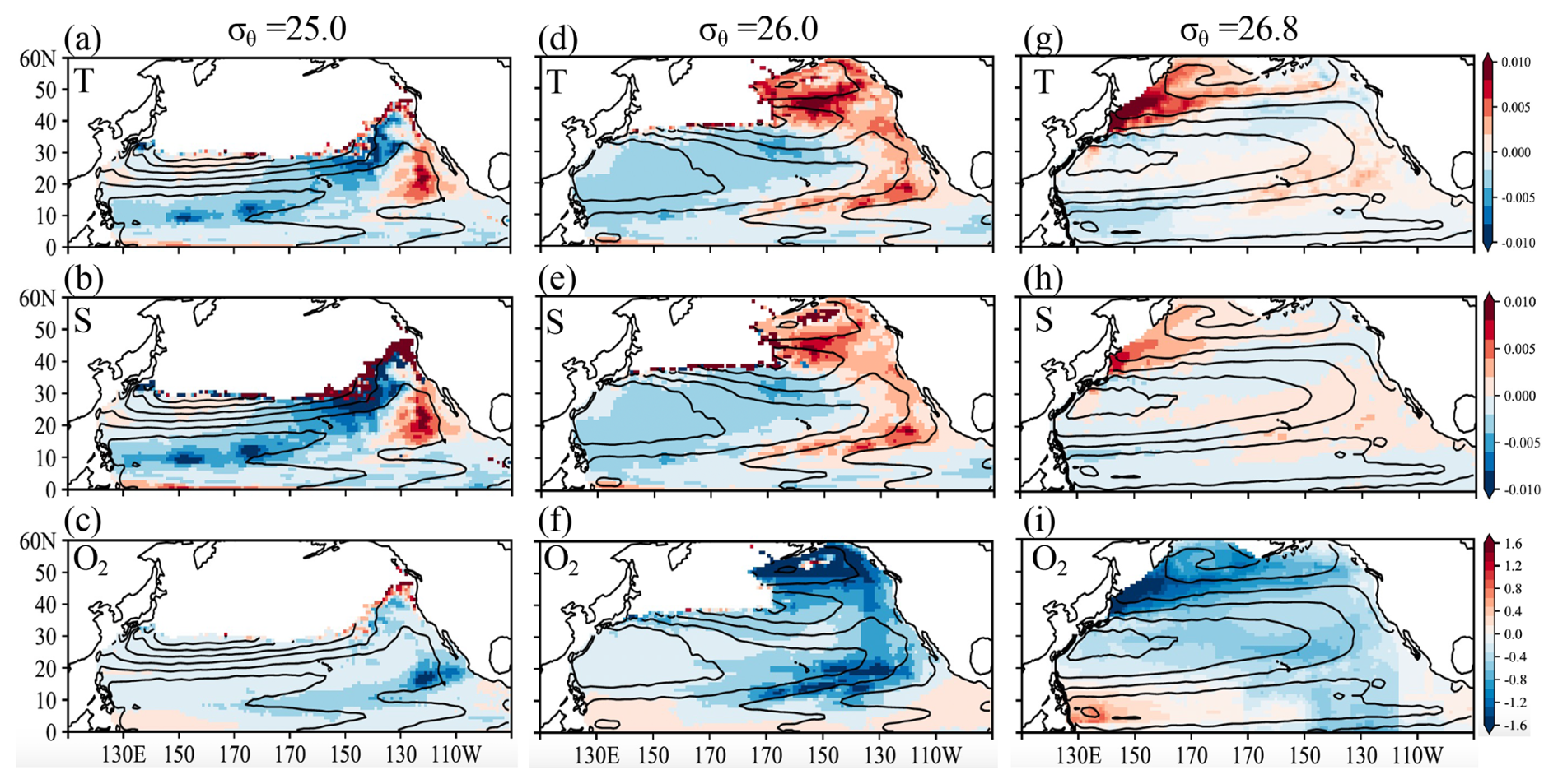
Figure 5 Linear trends in (a) potential temperature (° yr⁻¹), (b) salinity (1 yr⁻¹), and (c) dissolved O₂ (µmol kg⁻¹ yr⁻¹) on each isopycnal surface at 25.0, 26.0, and 26.8 σ_θ. Contour lines represent geostrophic flow streamlines on 26.0 and 26.8 σ_θ surfaces, relative to 2000 m.

The linear trends on the 25.0, 26.0, and 26.8 σ_θ surfaces show that positive and negative tendencies appear in characteristic locations and are generally aligned with the geostrophic streamlines (Fig. 5a–b, d–e, g–h). Although exceptions exist, such as weak positive trends (150–175° E, 20–30° N) (Fig. 5a–b), negative trends in potential temperature and salinity dominate in the western and central North Pacific on the 25.0 and 26.0 σ_θ surfaces (Fig. 5a–b, d–e). Conversely, positive trends in temperature and salinity are most prevalent in the northeastern and/or eastern regions of the basin along the geostrophic streamlines (Fig. 5a–b, d–e). These patterns suggest that waters subducted in the frontal region with reduced temperature and salinity originate mainly from the northeastern North Pacific and are advected southward along the subtropical circulation (Fig. 5a–b, d–e). Exceptions occur in parts of the northeastern basin (170–130° W, 40–60° N), where warmer and more saline waters influence the water masses sinking near the Alaska gyre and subsequently transported outside the subtropical gyre and along the California coast.

At 26.8 σ_θ (Fig. 5g–h), large positive trends in temperature and salinity are found along the Kuril Islands, with moderate positive trends appearing on the eastern side of the basin, respectively. Waters at this density range (26.8 σ_θ) are not directly ventilated but are formed through diapycnal mixing processes (Nakamura et al., 2000a, b; Nakamura and Awaji, 2004; You, 2003; Yasuda, 2004) and through double diffusion such as salt fingering (You, 2003). Thus, the observed positive temperature and salinity trends at 26.8 σ_θ likely reflect influences from changes occurring in the overlying layers (Fig. 5d–e and g–h).

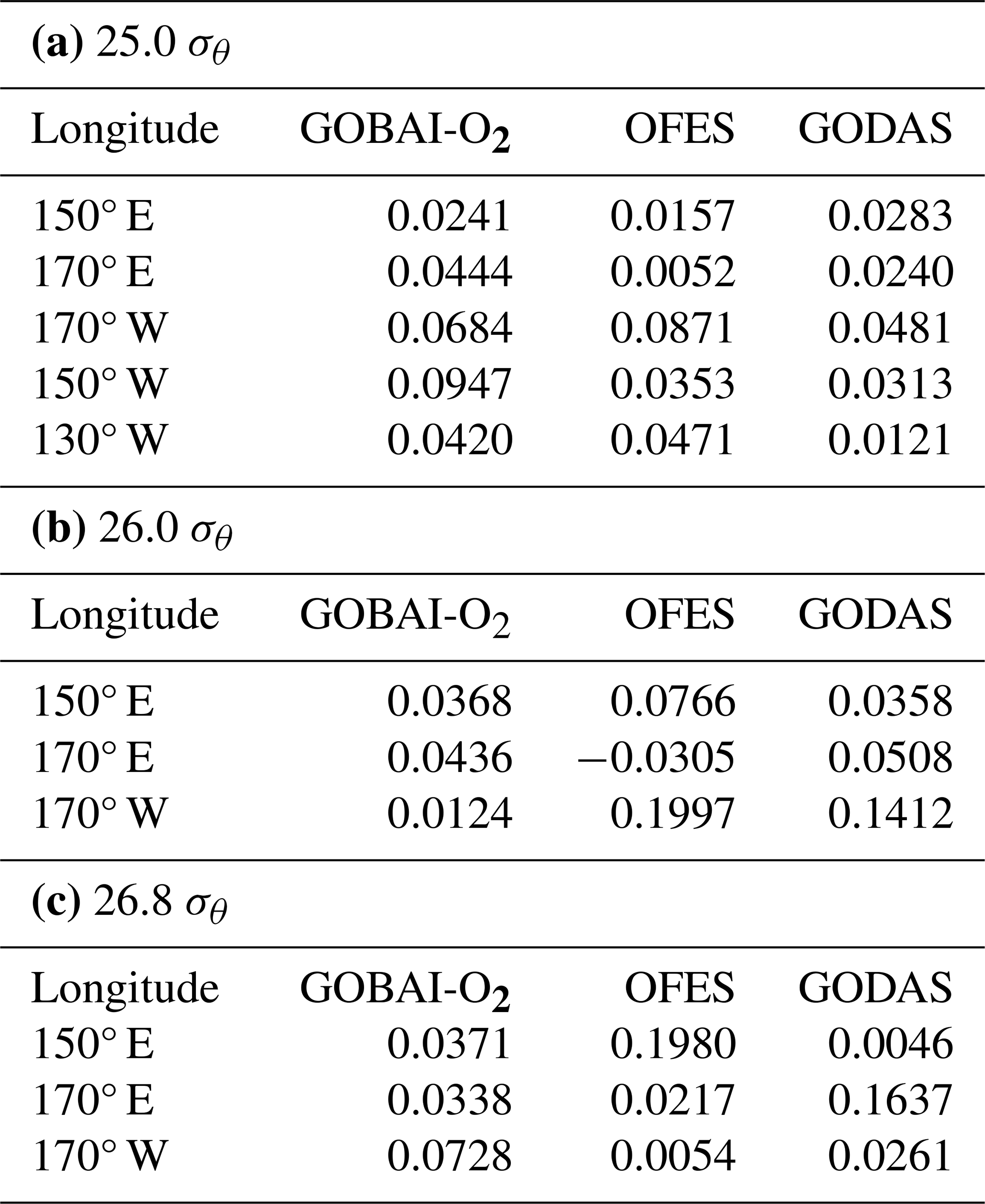
A meridional northward shift of the outcrop line in the North Pacific associated with recent climate change has been documented in OFES analyses (Ogata and Nonaka, 2020) and in other observational, reanalysis, and eddy-resolving ocean hindcasts (Xu et al., 2022). Consistent with these studies, the present dataset exhibits clear northward migration of the 25.0 σ_θ and 26.0 σ_θ outcrop lines (Fig. 6a), with the strong shifts occurring in the eastern basin between 150° E and 180° W (Fig. 6 and Table 1). The estimated northward shift rate at 0.004–0.09 ° yr⁻¹ from 2004 to 2023 is comparable to the value of 0.04 ° yr⁻¹ reported by Xu et al. (2022) for 1980 to 2018. Xu et al. (2022) further demonstrated that changes in the mixed layer and outcrop lines are tightly coupled with the northward migration of the North Pacific subtropical gyre and KE/OE fronts due to the poleward expansion of the Hadley cell, including the fact that the Kuroshio Extension and Oyashio Extension fronts, mode waters, and subtropical fronts evolve as a coherent system. These changes may also reflect the influence of anthropogenic warming, which has been linked to the poleward expansion of the Hadley circulation and the associated meridional shifts of oceanic fronts (Yang et al., 2020).

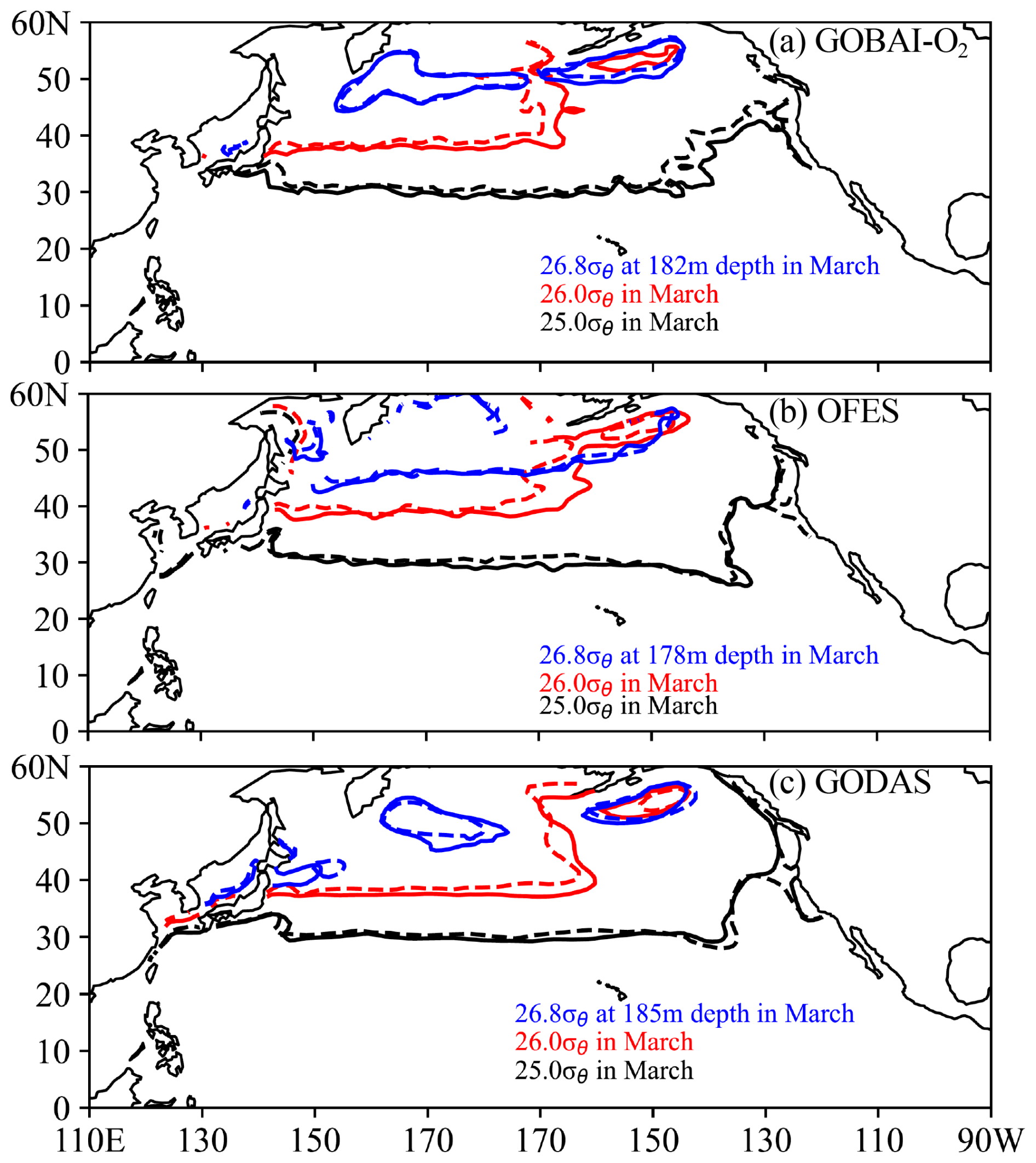
Figure 6 Density contours of 25.0 σ_θ (black), 26.0 σ_θ (red), and 26.8 σ_θ (blue) in each dataset: (a) GOBAI-O₂, (b) OFES, and (c) GODAS. Solid lines indicate the mean March density contours for 2004–2009, while dashed lines represent those for 2019–2023.

Table 1 Northern shifts of the (outcrop) isopycnal latitudes (° yr⁻¹) for 25.0 σ_θ (a), 26.0 σ_θ (b), and 26.8 σ_θ (c) in the GOBAI-O₂, OFES, and GODAS datasets. The estimates are based on data from March of each year. For 26.8 σ_θ, the northern shift is evaluated using the isopycnal depths corresponding to 182, 178, and 183 m in GOBAI-O₂, OFES, and GODAS, respectively.

Such poleward displacements of frontal structures can help explain the negative temperature and salinity trends in the subtropical gyre, where less saline subarctic-origin waters are subducted and advected southward. The positive temperature and salinity trends occurring in the Alaska region (160–130° W, 30–60° N) (Fig. 5a–b and d–e) are likewise consistent with the direct surface warming. In contrast, the 26.0 σ_θ front exhibits primarily longitudinal, rather than meridional, shifts between 2004 and 2023 (Fig. 6), suggesting that the associated temperature and salinity changes arise mainly from direct surface warming and freshening, rather than from density-compensated shifts in water-mass distribution.

3.3.2 Dissolved oxygen

The linear trends in dissolved oxygen on the isopycnal surfaces at 25.0, 26.0, and 26.8 σ_θ exhibit predominantly negative values across the North Pacific (Fig. 5c, f, and i), although their spatial distributions are not uniform. Large negative trends are concentrated in the northeastern and eastern regions and gradually decrease toward the west (Fig. 5c, f, and i). Exceptions occur mainly in the tropics, where notable positive trends are found in the western tropical areas on the 26.0 and 26.8 σ_θ surfaces.

The temporal changes in dissolved oxygen (O₂) were decomposed following the method of Sasano et al. (2015). The processes underlying the oxygen tendency equations (Eqs. 2 and 3) are summarized below. We evaluated each contributing term and examined its relative importance for the dissolved O₂ trends. The total tendency of dissolved oxygen can be expressed as

$$\begin{array}{}\text{(2)}& {\displaystyle \frac{\partial {\mathrm{O}}_{\mathrm{2}}}{\partial t}}=\left({\displaystyle \frac{\partial {\mathrm{O}}_{\mathrm{2}}}{\partial z}}{\displaystyle \frac{\partial z}{\partial t}}\right)+{\left({\displaystyle \frac{\partial {\mathrm{O}}_{\mathrm{2}}^{\mathrm{sat}}}{\partial t}}\right)}_{\mathrm{net}}-{\left({\displaystyle \frac{\partial \left(\mathrm{AOU}\right)}{\partial t}}\right)}_{\mathrm{net}},\end{array}$$

which can be rearranged as

$$\begin{array}{}\text{(3)}& \begin{array}{rl}\begin{array}{c}{\displaystyle \frac{\partial {\mathrm{O}}_{\mathrm{2}}}{\partial t}}\\ \left(\mathrm{i}\right)\end{array}& =\begin{array}{c}\left({\displaystyle \frac{\partial {\mathrm{O}}_{\mathrm{2}}}{\partial z}}{\displaystyle \frac{\partial z}{\partial t}}\right)\\ \left(\mathrm{ii}\right)\end{array}+(\begin{array}{c}{\displaystyle \frac{\partial {\mathrm{O}}_{\mathrm{2}}^{\mathrm{sat}}}{\partial t}}\\ \left(\mathrm{iii}\right)\end{array}-\begin{array}{c}{\displaystyle \frac{\partial {\mathrm{O}}_{\mathrm{2}}^{\mathrm{sat}}}{\partial z}}{\displaystyle \frac{\partial z}{\partial t}}\\ \left(\mathrm{iv}\right)\end{array})\\ & +(-\begin{array}{c}{\displaystyle \frac{\partial \left(\mathrm{AOU}\right)}{\partial t}}\\ \left(\mathrm{v}\right)\end{array}+\begin{array}{c}{\displaystyle \frac{\partial \left(\mathrm{AOU}\right)}{\partial z}}{\displaystyle \frac{\partial z}{\partial t}}\\ \left(\mathrm{vi}\right)\end{array}).\end{array}\end{array}$$

Here, X=O₂, O${}_{\mathrm{2}}^{\mathrm{sat}}$, AOU (Apparent Oxygen Utilization). The term $\partial z/\partial t$ denotes the temporal change in the depth of the isopycnal surface (z), while $\partial X/\partial z$ represents the vertical gradient of the variable X at that surface, averaged over the past 20 years. The net tendency term ($\partial X/\partial t{)}_{\mathrm{net}}$ represents the net changes associated with a variable X.

By applying Eq. (3), the rate of O₂ change (term i), which is the rate of reconstructed O₂ data estimated from the linear regression analysis, on each isopycnal surface can be decomposed into contributions from:

• (term ii) vertical heave acting on the vertical O₂ gradient;

• (term iii) solubility effects due to temperature and salinity changes;

• (term iv) vertical heave acting on the solubility gradient;

• (term v) AOU changes related to air-sea disequilibrium, biological activities, and lateral circulation

• (term vi) vertical heave acting on AOU gradients.

The derivation of Eqs. (2) and (3) follows Sasano et al. (2015) and is described in Appendix A. A schematic illustration of this decomposition is provided in Fig. S5.

Figure 7 shows the horizontal distributions of the magnitude of each term on 25.0, 26.0, and 26.8 σ_θ surfaces. The results indicate that the prominent O₂ declines (Fig. 5c, f, i) arise from a combination of positive and negative contributions, with the dominant terms varying by latitude. In the high-latitude region around the Alaska Gyre (170–130° W, 40–60° N), the largest negative contributions are associated with the deepening of isopycnal surfaces (term ii) and the vertical heave acting on the AOU gradient (term vi) (Fig. 7f, j, k, o). Because the dissolved oxygen generally decreases with depth ($\partial O_{\mathrm{2}}/\partial z<\mathrm{0}$), deepening of isopycnal surfaces ($\partial z/\partial t>\mathrm{0}$) (Fig. 8b–c) produces a negative contribution through vertical heave. Similarly, because AOU typically increases with depth, isopycnal deepening leads to an apparent increase in AOU, contributing negatively to dissolved O₂ via term (vi). In contrast, solubility-related changes (term iii) and net AOU tendencies (term v) act in opposite directions during this period (Fig. 7g–h, l–m). Taken together, these results are consistent with the strong negative O₂ trends observed in the Bering Sea on the 26.0 σ_θ and 26.8 σ_θ surfaces (150° E–170° W, 50–60° N; Fig. 5f and i).

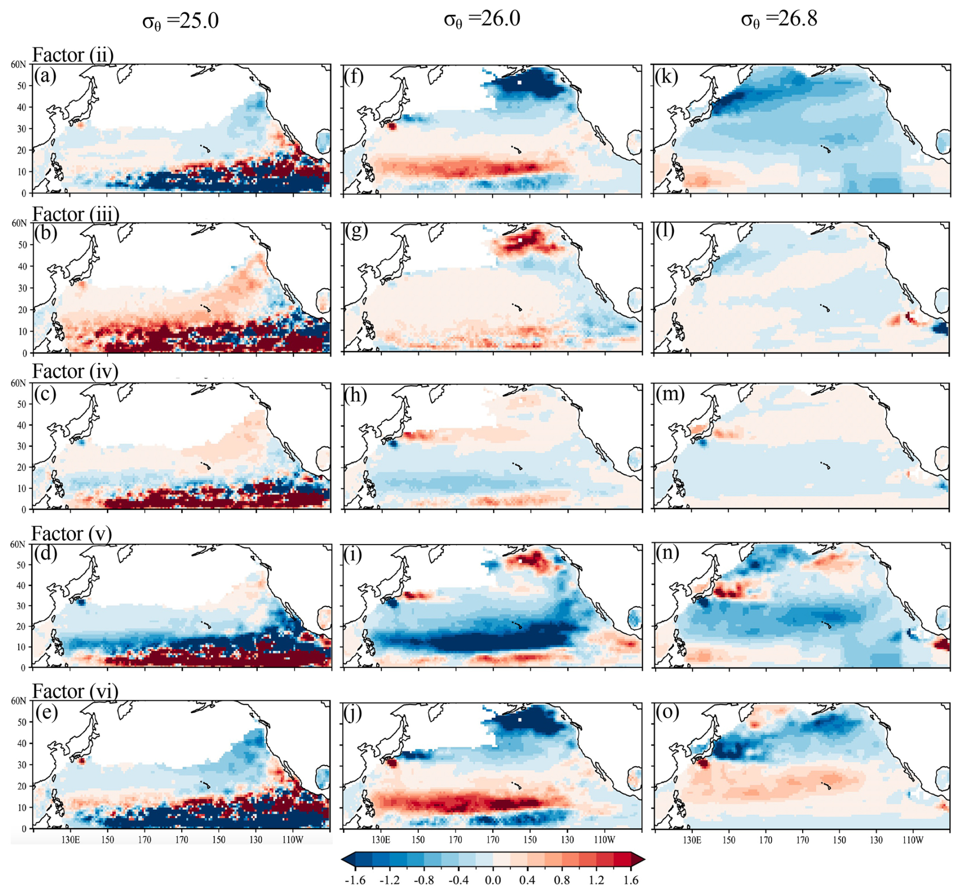
Figure 7 Horizontal distributions of the changing rates (µmol kg⁻¹ yr⁻¹) of each factor contributing to the rate of O₂ change on 25.0, 26.0, and 26.8 σ_θ in Eq. (1). The rate of O₂ change on each isopycnal surface is decomposed into the following components: (ii) the apparent contribution from vertical heave (deepening or shoaling) of isopycnal surfaces associated with warming and/or surface freshening; (iii) the contribution from changes in oxygen solubility (O${}_{\mathrm{2}}^{\mathrm{sat}}$) associated with temperature and salinity variations; (iv) the contribution from vertical heave acting on the background solubility gradient; (v) the contribution from net changes in apparent oxygen utilization (AOU) associated with air–sea disequilibrium, biological activity, and lateral advection and/or circulation; and (vi) the contribution from vertical heave acting on AOU gradients, independent of solubility changes. This decomposition is applied to the reconstructed dissolved oxygen fields obtained from linear regression analysis.

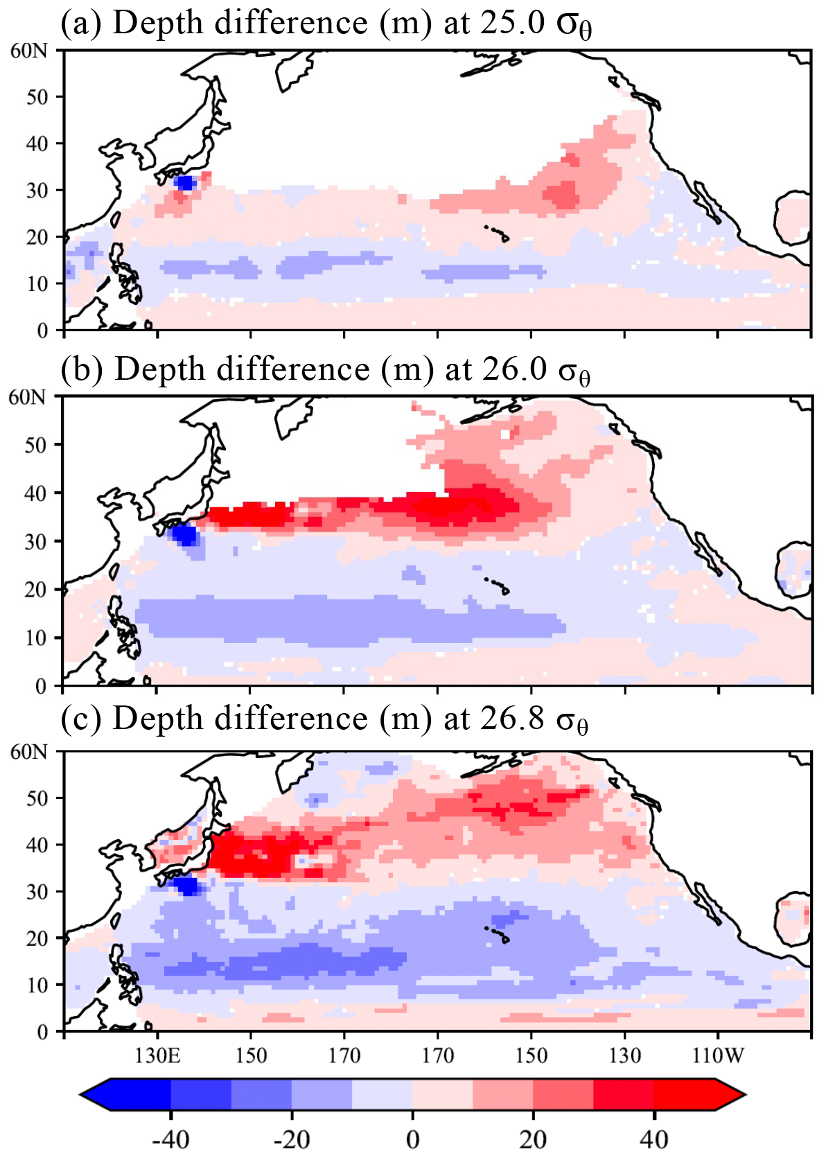
Figure 8 Depth difference (m) between the 5-year averaged data in March, 2004–2009 and 2018–2023 at 25.0, 26.0, and 26.8 σ_θ. The reconstructed O₂ data estimated from the linear regression analysis were used in this calculation. Positive and negative values indicate the deepening and shallowing, respectively, from the depth of each density in 2004–2023.

In the subtropical and mid-latitudes (10–40° N), the O₂ decline is largely associated with AOU changes (term v) (Fig. 7d, i, and n). The relative weakening of the total O₂ decrease in the western North Pacific (Fig. 5c, f, i) coincides with positive contributions from vertical heave of isopycnal surfaces (term ii) (Fig. 7f and k). Additional positive trends arise from solubility-related effects (term iii) (Fig. 7b), and the vertical heave acting on the AOU gradient (term vi) (Figs. 7j and o and 8b–c).

In the mid-ocean between 170° E and 160° W, the positive O₂ tendencies transition to weakly negative values. In contrast, a pronounced band of positive trends is found zonally across the North Pacific Ocean between 30 and 50° N, primarily associated with the combined effects of terms (iii) and (v) (Fig. 7l, h–i, and m–n). This pattern may be related to the northward meridional shift of the subtropical and subarctic frontal zone under recent global warming (Ogata and Nonaka, 2020). Enhanced winter convection in this region may introduce nutrients into the surface layer, potentially increasing biological activity and AOU. In the NPIW formation region near the Kuril Islands, negative contributions from term (iii) are observed (Fig. 7l), suggesting weaker vertical mixing during the observational period, likely influenced by enhanced surface-layer stratification. This interpretation is supported by the positive trends in temperature and salinity observed in the winter subducted areas (Suga et al., 1997, 2004; Yasuda, 2004) (Fig. 5d–e, g–h).

In the western tropical Pacific, pronounced increases in dissolved O₂ are observed within the density range of 26.8–27.2 σ_θ (Figs. 3c and g; 4c and g; 5c, f, and i), overlapping with the OML (Reid, 1997). Similar features have been reported by Sasano et al. (2015) and Takatani et al. (2012). Variability of the North Equatorial Counter Current (NECC) is likely relevant in this region. According to the study of Chen et al. (2016) based on the OFES outputs including a multidecadal variability (1960–2014), the NECC exhibits two distinct modes of variability: an interannual mode characterized by strengthening accompanied by southward migration, and an interdecadal mode marked by a gradual weakening, poleward migration, and broadening.

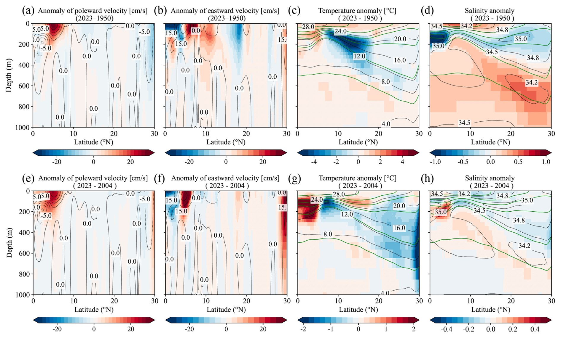
Figure 9 Anomaly of poleward and eastward velocity, potential temperature, and salinity in the OFES model outputs from 1950 to 2023 (a–d) and from 2004 to 2023 (e–h), respectively, in the 137° E line. Contours of averaged values of poleward and eastward velocity, potential temperature, and salinity during the target period are also shown in each figure. Green contour lines in (c)–(d), (g)–(h) indicate the average potential density of 22, 23, 24, 25, 26, and 27 σ_θ, during the target periods.

The validity of time-varying signals in the western tropical Pacific in the OFES data has been demonstrated by Chen et al. (2016). We further examined the longer-term OFES data (1950–2023), as well, for poleward, eastward velocities, as well as potential temperature and salinity here (Fig. 9c, g). Positive temperature anomalies in 0–5° N occur above 250 m depth, while negative anomalies appear along the 26.0 σ_θ surface between 5–20° N, a similar pattern that is also evident in the GOBAI-O₂ data (Fig. 3a). A discrepancy is found in salinity trends: GOBAI-O₂ shows negative trends along 26.0 σ_θ (Fig. 3b), whereas OFES exhibits positive trends (Fig. 9b, f), likely reflecting higher salinity at 200–600 m depth in OFES between 0 and 7° N (Fig. 10b, d).

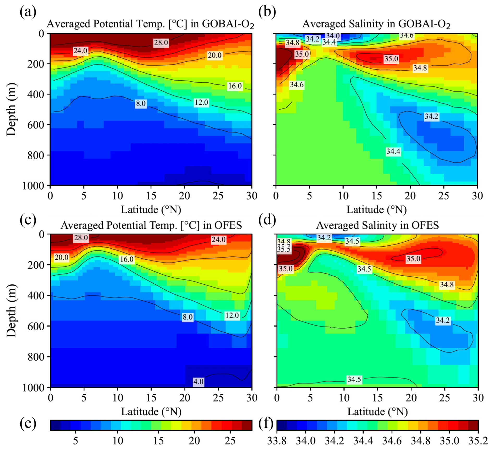
Figure 10 Averaged Potential Temperature (a, c) and salinity (b, d) in GOBAI-O₂ from 2004 to 2023 and OFES data from 1950 to 2023, respectively, in the 137° E line.

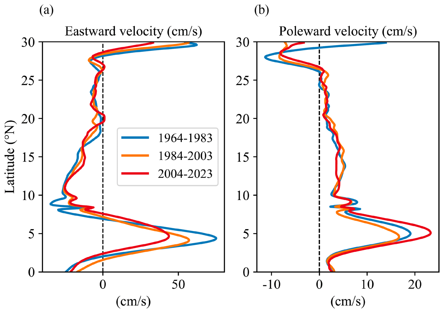
Figure 11 Latitudinal distribution of averaged eastward (a) and poleward velocity (b) in the OFES data from 1964 to 1983, from 1984 to 2003, and from 2004 to 2023, respectively, in the 137° E line.

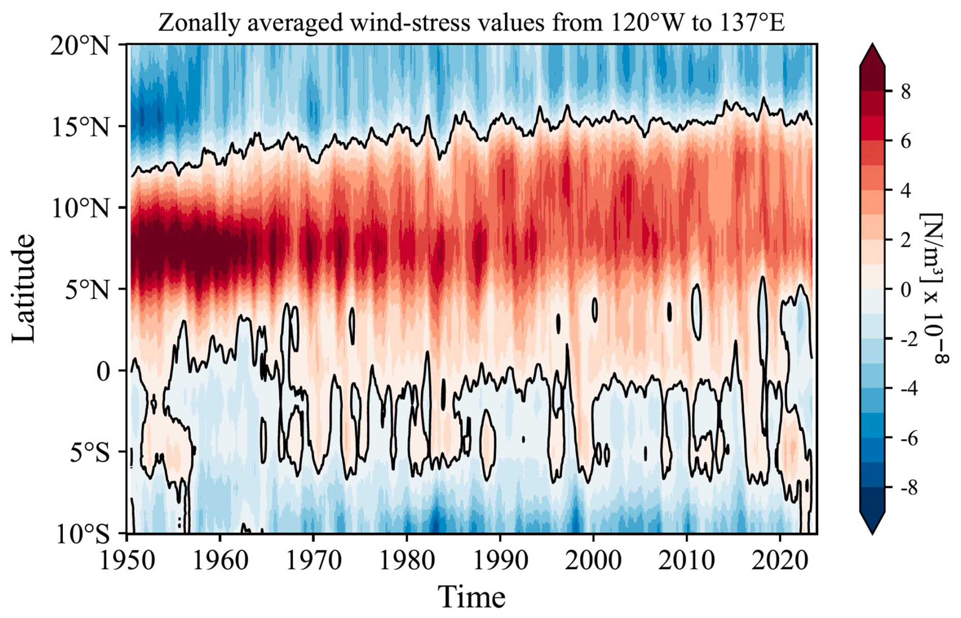
Figure 12 NCEP-NCAR wind-stress curl values zonally averaged from 137° E to 120° W from 1950 to 2023. A 13-month running-mean filter has been applied in time.

Anomalies in poleward and eastward velocities (Figs. 9a–b, e–f and 11a–b) indicate enhanced poleward flow around 5° N above 200 m depth and a poleward shift of the eastward velocity core. These changes are consistent with the interdecadal mode of NECC variability described by Chen et al. (2016). The broadening of the NECC was less evident here, possibly because the present analysis uses raw velocity fields rather than isolating the second EOF modes. The wind-stress curl over the equatorial Pacific shows a persistent decrease and poleward expansion of negative values along the 0–10° N from 1950 to 2023 (Fig. 12).

The westward penetration of the OML is slow and occurs between two eastward-extending tongues of high O₂ water originating near the equator (Reid, 1997) (Fig. S6). The observed O₂ increase on the 26.8–27.2 σ_θ surfaces (Figs. 3c, g and 4c, g) is consistent with a weakening and northward shift of the interdecadal NECC mode. The subsurface O₂ increase, particularly below 400 m depth (Fig. 1r–u), is therefore likely influenced by these circulation changes, potentially allowing higher-O₂ water to extend westward (Fig. S6). In addition, shoaling of isopycnal surfaces near the equator indicates a northward shift of the boundary between the tropical and subtropical gyres along 137° E line during the observational period.

4 Discussion and Conclusion

The variability of dissolved oxygen in the North Pacific reflects the combined influences of global warming and climate variability. In this study, we used the four-dimensional GOBAI-O₂ dataset, constructed using machine–learning methods applied to historical temperature, salinity, and oxygen observations from BGC-Argo floats and ship-based measurements – to examine linear trends in potential temperature, salinity, and dissolved oxygen over the past two decades (2004–2023). The linear trends are broadly consistent with findings from previous studies (Takatani et al., 2012; Sasano et al., 2015; Ogata and Nonaka, 2020), and we clarified how these trends vary spatially (Figs. 3 and 4).

An important outcome of this study is that GOBAI-O₂, being globally gridded, allows spatially continuous and smooth representations of trends, both horizontally and vertically, across the North Pacific. This provides a more spatially coherent representation than earlier datasets that relied solely on sparse ship-based observations. The horizontal trend patterns mapped on isopycnal surfaces (Fig. 5) show that dissolved oxygen exhibits a basin-scale decreasing trend. At the same time, several regions display locally increasing oxygen, including areas influenced by the meridional migration of subtropical and subpolar fronts (Fig. 4). The strong positive oxygen trends in the western equatorial region are consistent with a weakening of the second mode of the NECC variability. The decomposition analysis further illustrates how each physical component contributes to oxygen changes along isopycnal surfaces (Fig. 7).

Although many of the large-scale features identified here resemble those reported by Ito et al. (2017), our analysis reveals regional and isopycnal-scale structures that were previously unresolved. In particular, the positive oxygen trends in the Kuroshio–Oyashio Transition Zone, the northeastern North Pacific along the 26.8–27.0 σθ density surfaces, and the enhanced subsurface O₂ increase in the tropical western Pacific below 400 m were not clearly distinguished in earlier O₂ anomaly studies. These improvements arise because GOBAI-O₂ integrates high-frequency BGC-Argo oxygen observations with a spatially consistent mapping scheme, reducing observational gaps and sampling biases in dynamically active regions. This suggests that regional reoxygenation signals can coexist with large-scale deoxygenation, and highlights the importance of sustained BGC-Argo observations for detecting emerging changes in ocean biogeochemistry.

Recent work by Bushinsky et al. (2025) has reported the presence of a systematic negative bias (approximately −2.7 µmol kg⁻¹) in air-calibrated BGC-Argo oxygen measurements compared with ship-based reference profiles. This bias does not appear to be explicitly corrected in version 4.4 of GOBAI-O₂-v2.2 and may therefore influence the magnitude of the estimated oxygen trends–potentially enhancing negative trends or suppressing positive ones in regions with dense float sampling. However, as described in Sect. 2.1, a substantial fraction of these float data is subject to quality control through comparison with climatological fields derived from ship-based discrete observations, and only profiles with appropriate quality flags are retained and incorporated into the dataset development. While this filtering procedure likely mitigates a portion of the air-calibration bias, the extent to which residual bias remains in the reconstructed fields is not well quantified.

If present, such biases could also affect the apparent vertical structure of the oxycline. In the North Pacific, regions with high float density–such as the Kuroshio–Oyashio transition zone, the North American coastal region, and the vicinity of Hawaii–may be particularly affected (see Fig. 1 of Sharp et al., 2023). While a constant offset would not directly alter linear trend estimates, any time–varying bias associated with sensor behavior or sampling depth could introduce spurious trends. A quantitative evaluation is not feasible at present due to the lack of temporally continuous ship-based reference data at the spatial scales. This limitation should therefore be kept in mind when interpreting the O₂ trends reported here. Accordingly, the interpretation of the diagnosed O₂ trends should be made with caution, particularly in regions where float-based observations dominate.

It is also essential to recognize that GOBAI-O₂ is a machine learning reconstruction derived from available temperature, salinity, and oxygen measurements. While this approach significantly enhances spatial coverage, the results should be interpreted cautiously. In particular, although the large-scale spatial patterns are broadly consistent across datasets, both the magnitude of trends and finer-scale spatial features may still be affected by unresolved observational and reconstruction uncertainties. Nevertheless, future work incorporating improved calibration of Argo oxygen sensors, expanded ship-based reference datasets, independent machine learning reconstructions (e.g., Ito et al., 2024), and comprehensive ocean reanalysis will be necessary to better constrain these uncertainties.

Different versions of the GOBAI-O₂ product may yield different oxygen trend estimates because of methodological differences among releases. Therefore, some of the regional patterns discussed in this study may be sensitive to the specific GOBAI-O₂ version used in the analysis. Future comparisons across multiple GOBAI-O₂ versions and observational products would help further assess the robustness of the results. The monthly mean climatological GOBAI-O₂ dataset should include the Pacific Decadal Oscillation (PDO; Stramma et al., 2020; Pozo Buil and Di Lorenzo, 2017) and the North Pacific Gyre Oscillation (NPGO; Stramma et al., 2020). This dataset, therefore, provides a valuable basis for examining how such climate variability influences dissolved oxygen through physical driving mechanisms. Investigating these relationships more explicitly will be an important direction for future research.

Appendix A: Essential concepts and derivations for Eqs. (2)–(3)

The essential concepts and derivations for Eqs. (2) and (3) were originally proposed by Takatani et al. (2012) and subsequently described in detail by Sasano et al. (2015). Here, we briefly summarize and follow their derivation.

When the temperature at a depth z_A increases from θ_A to ${\mathit{\theta }}_A^{\prime }$ as a result of increased ocean heat content, the density at that depth decreases from σ_A to ${\mathit{\sigma }}_A^{\prime }$. For simplicity, the vertical salinity profile is assumed to remain unchanged with time. As a consequence, the isopycnal surface of σ_A deepens from z_A to z_B (Fig. S5). If surface freshening occurs simultaneously due to a net freshwater input, both the density decreases at z_A (from σ_A to ${\mathit{\sigma }}_A^{\prime }$) and the deepening of the isopycnal surface (from z_A to z_B) are enhanced. Because density is a function of temperature and salinity (σ=f(θS)), the density of the isopycnal surface σ_A can be expressed as

$$\begin{array}{}\text{(A1)}& {\displaystyle }{\mathit{\sigma }}_A=f\left({\mathit{\theta }}_A{S}_A\right)\left(\mathrm{before}\mathrm{warming}\right)\text{(A2)}& {\displaystyle }=f({\mathit{\theta }}_B^{\prime },S_B)\left(\mathrm{after}\mathrm{warming}\right).\end{array}$$

Here, S_A and S_B denote salinity at depth z_A and z_B, respectively, and ${\mathit{\theta }}_B^{\prime }$ represents the temperature at density σ_A at depth z_B after warming. The depth z_B is determined by satisfying Eqs. (A1) and (A2). In the region where salinity decreases with depth (e.g., above the salinity minimum layer of NPIW), S_A>S_B, and therefore ${\mathit{\theta }}_A\mathit{>}{\mathit{\theta }}_B^{\prime }$. This implies that the potential temperature on an isopycnal surface effectively decreases as a consequence of warming, and that biogeochemical properties on the same isopycnal surface are also expected to change.

For a tracer X whose vertical profile with respect to depth does not change with time (e.g., salinity; see Fig. S5c), the temporal change of X on the potential density surface σ_A is attributed solely to the apparent change caused by the deepening of the isopycnal surface from z_A to z_B:

$$\begin{array}{}\text{(A3)}& {\displaystyle \frac{\partial X}{\partial t}}=\left({\displaystyle \frac{\partial X}{\partial z}}\cdot {\displaystyle \frac{\partial z}{\partial t}}\right)\end{array}$$

Here, $\partial X/\partial t$ represents the temporal change of X observed on σ_A (gray arrows in Fig. S5), z denotes the depth of σ_A, $\partial X/\partial z$ is the vertical gradient of X with respect to the depth (assumed to be time-invariant), and $\partial z/\partial t$ is the rate of deepening of the isopycnal surface σ_A. The product $\partial X/\partial z\cdot \partial z/\partial t$ represents the effect of isopycnal deepening (white arrows in Fig. S5), corresponding to the difference between the filled square and filled circle.

For a variable Y whose vertical profile evolves with time while warming occurs simultaneously, the temporal change of Y on the density surface σ_A can be expressed as the sum of two components: the contribution due to the isopycnal deepening from z_A to z_B and the net temporal change of Y, ($\partial Y/\partial t{)}_{\mathrm{net}}$ between the time before and after warming:

$$\begin{array}{}\text{(A4)}& {\displaystyle \frac{\partial Y}{\partial t}}=\left({\displaystyle \frac{\partial Y}{\partial z}}\cdot {\displaystyle \frac{\partial z}{\partial t}}\right)+{\left({\displaystyle \frac{\partial Y}{\partial t}}\right)}_{\mathrm{net}}\end{array}$$

To evaluate the net change ($\partial Y/\partial z{)}_{\mathrm{net}}$ (illustrated by the blue arrows of a difference in symbols between filled square and open square in Fig. S5), it is necessary to evaluate the contribution of the temporal change of Y due to the isopycnal deepening and to subtract it from the change of Y observed at density σ_A. For instance, the change of O${}_{\mathrm{2}}^{\mathrm{sat}}$ in Fig. S5f is observed along the gray isopycnal surface (large white arrow), whereas the net change (large blue and pink arrows) is obtained as the difference between the observed change and the deepening effect.

The dissolved oxygen concentration O₂ can be expressed as:

$$\begin{array}{}\text{(A5)}& {\mathrm{O}}_{\mathrm{2}}={\mathrm{O}}_{\mathrm{2}}^{\mathrm{sat}}-\mathrm{AOU},\end{array}$$

where O${}_{\mathrm{2}}^{\mathrm{sat}}$ is the oxygen saturation concentration (a function of temperature and salinity), and AOU is “apparent oxygen utilization”, representing the oxygen consumed by biological processes since subduction. Near the surface, AOU is typically small, and its contributions can be neglected.

Following Eq. (A4), the temporal change of O₂ on a given isopycnal surface at a fixed station is:

$$\begin{array}{}\text{(A6)}& {\displaystyle \frac{\partial {\mathrm{O}}_{\mathrm{2}}}{\partial t}}=\left({\displaystyle \frac{\partial {\mathrm{O}}_{\mathrm{2}}}{\partial z}}\cdot {\displaystyle \frac{\partial z}{\partial t}}\right)+{\left({\displaystyle \frac{\partial {\mathrm{O}}_{\mathrm{2}}}{\partial t}}\right)}_{\mathrm{net}}.\end{array}$$

Similarly,

$$\begin{array}{}\text{(A7)}& {\displaystyle \frac{\partial {\mathrm{O}}_{\mathrm{2}}^{\mathrm{sat}}}{\partial t}}=\left({\displaystyle \frac{\partial {\mathrm{O}}_{\mathrm{2}}^{\mathrm{sat}}}{\partial z}}\cdot {\displaystyle \frac{\partial z}{\partial t}}\right)+{\left({\displaystyle \frac{\partial {\mathrm{O}}_{\mathrm{2}}^{\mathrm{sat}}}{\partial t}}\right)}_{\mathrm{net}},\end{array}$$

and

$$\begin{array}{}\text{(A8)}& {\displaystyle \frac{\partial \mathrm{AOU}}{\partial t}}=\left({\displaystyle \frac{\partial \left(\mathrm{AOU}\right)}{\partial z}}\cdot {\displaystyle \frac{\partial z}{\partial t}}\right)+{\left({\displaystyle \frac{\partial \left(\mathrm{AOU}\right)}{\partial t}}\right)}_{\mathrm{net}}.\end{array}$$

The term net is directly related to warming, because depends on temperature and salinity. If AOU does not change with time, that is, if changes in O₂ arise solely from changes in, then $\partial \left(\mathrm{AOU}\right)/\partial t$ follows Eq. (A3) and =0. If AOU varies with time, however, $\partial \left(\mathrm{AOU}\right)/\partial t$ follows Eq. (A4) and ≠0, as illustrated by the dashed gray line in Fig. S5g.

Because O₂ is defined by Eq. (A5), the net temporal change of O₂ on an isopycnal surface is

$$\begin{array}{}\text{(A9)}& {\left({\displaystyle \frac{\partial {\mathrm{O}}_{\mathrm{2}}}{\partial t}}\right)}_{\mathrm{net}}={\left({\displaystyle \frac{\partial {\mathrm{O}}_{\mathrm{2}}^{\mathrm{sat}}}{\partial t}}\right)}_{\mathrm{net}}-{\left({\displaystyle \frac{\partial \left(\mathrm{AOU}\right)}{\partial t}}\right)}_{\mathrm{net}}.\end{array}$$

Combining Eqs. (A6) and (A9), the total temporal change of O₂ on an isopycnal surface can be written as

$$\begin{array}{}\text{(A10)}& \left({\displaystyle \frac{\partial {\mathrm{O}}_{\mathrm{2}}}{\partial t}}\right)=\left({\displaystyle \frac{\partial {\mathrm{O}}_{\mathrm{2}}}{\partial z}}\cdot {\displaystyle \frac{\partial z}{\partial t}}\right)+{\left({\displaystyle \frac{\partial {\mathrm{O}}_{\mathrm{2}}^{\mathrm{sat}}}{\partial t}}\right)}_{\mathrm{net}}-{\left({\displaystyle \frac{\partial \left(\mathrm{AOU}\right)}{\partial t}}\right)}_{\mathrm{net}},\end{array}$$

which corresponds to Eq. (1) in the main text. Equation (A10) corresponds to an arrow in Fig. S5e, represented from left to right by the large gray arrow, white, blue, and pink arrows. The large blue arrow is identical to Fig. S5f, while the large pink arrow corresponds to Fig. S5g, but with its direction reversed. Finally, substituting Eqs. (A7) and (A8) into (A10)

$$\begin{array}{}\text{(A11)}& \begin{array}{rl}\begin{array}{c}{\displaystyle \frac{\partial {\mathrm{O}}_{\mathrm{2}}}{\partial t}}\\ \left(\mathrm{i}\right)\end{array}& =\begin{array}{c}\left({\displaystyle \frac{\partial {\mathrm{O}}_{\mathrm{2}}}{\partial z}}{\displaystyle \frac{\partial z}{\partial t}}\right)\\ \left(\mathrm{ii}\right)\end{array}+\begin{array}{c}({\displaystyle \frac{\partial {\mathrm{O}}_{\mathrm{2}}^{\mathrm{sat}}}{\partial t}}\\ \left(\mathrm{iii}\right)\end{array}-\begin{array}{c}{\displaystyle \frac{\partial {\mathrm{O}}_{\mathrm{2}}^{\mathrm{sat}}}{\partial z}}{\displaystyle \frac{\partial z}{\partial t}})\\ \left(\mathrm{iv}\right)\end{array}\\ & -(\begin{array}{c}{\displaystyle \frac{\partial \left(\mathrm{AOU}\right)}{\partial t}}\\ \left(\mathrm{v}\right)\end{array}-\begin{array}{c}{\displaystyle \frac{\partial \left(\mathrm{AOU}\right)}{\partial z}}{\displaystyle \frac{\partial z}{\partial t}}\\ \left(\mathrm{vi}\right)\end{array}),\end{array}\end{array}$$

which corresponds to Eq. (2) in the main text. Note: The signs in terms (v) and (vi) in Eq. (3) are reversed relative to those in Eq. (A11) for convenience.

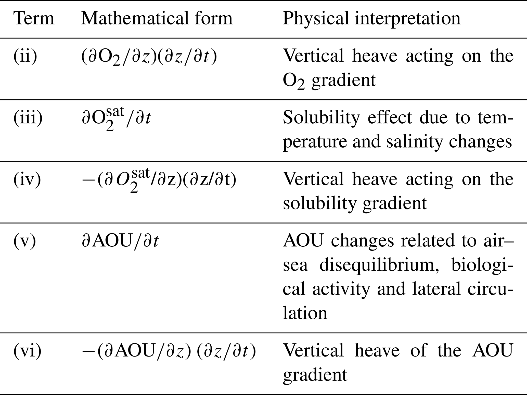
Table A1 The physical interpretation of each term in the oxygen tendency decomposition shown in Eqs. (3) and (A11) is summarized.