Prediction of present and future spatial occurrence of cyanobacteria and the toxin nodularin in the Baltic Sea

Blooms of filamentous cyanobacteria are recurrent phenomena in the brackish Baltic Sea. These blooms can contain toxin-producing strains. However, predicting and modeling the toxins spatial distribution poses great challenges. In addition, projected rising temperature due to climate change may increase the occurrence of cyanobacterial blooms, making it vital to understand the distribution of the blooms and the associated cyanotoxins. Herein, using a conceptual modeling setup, we integrated the measured concentration of the cyanotoxin nodularin, the abundance of the toxin producer Nodularia spumigena, and environmental variables using Empirical Bayesian Kriging (EBK) prediction, ensemble learning, and stacked species distribution modeling (SSDM). This conceptual modeling setup was used to predict and interpret the current and future area distribution of N. spumigena and nodularin across the Baltic Sea. Predictions were based on results from biogeochemical models describing current and projected future concentrations of near-surface chlorophyll, nitrate, phosphate, salinity, and temperature along with nitrate-to-phosphate ratio and the geographical variable distance to shore. Prediction for the future distribution was performed using projected climate change scenarios in the year 2100. Findings show that the predicted area distribution of nodularin is determined by concentrations and interaction effects of salinity, temperature, phosphate, nitrate-to-phosphate ratio, and distance to shore, and is associated with the predicted area distribution of N. spumigena. Predicted site distribution shows increased nodularin occurrences in the Eastern and Western Gotland Sea, the Northern Baltic Proper, southern parts of the Bothnian Sea, and the Arkona basin. By the year 2100, area distribution of nodularin is predicted to increase in the northern part of the Eastern Gotland Sea, Northern Baltic Proper, Åland Sea, southern parts of the Bothnian Sea, Arkona Basin, and slightly into the Bothnian Bay in response to projected climate change scenarios. Our conceptual modeling approach is useful where toxicological data such as cyanotoxins are insufficient.

1 Introduction

Blooms of filamentous cyanobacteria occur regularly in the Baltic Sea during summer (Kahru et al., 2020; Kahru and Elmgren, 2014; Karlson et al., 2022), mainly from end of June until August, and are dominated by the diazotrophic filamentous cyanobacterial species Nodularia spumigena, Aphanizomenon flos-aquae, and Dolichospermum spp. (Carlsson and Rita, 2019; Klawonn et al., 2016; Olofsson et al., 2020a). The toxicity of these blooms is mainly attributed to the hepatotoxin nodularin, produced by N. spumigena. The chemical structure and toxicity of nodularin is similar to microcystin (Lundholm et al., 2009). The toxicity of cyanobacterial blooms is known to cause economic losses to the surrounding societies of the Baltic Sea (Jonasson et al., 2008) with negative effects on the food chain dynamics on several trophic levels (Karjalainen et al., 2007). How cyanobacteria and their toxins respond to the ongoing and future climate change in the Baltic Sea is, however, not well known. Therefore, an understanding of what influences and predicts the spatial occurrence of cyanobacteria and related toxins is needed for efficient management of the Baltic Sea.

The spatial and temporal distribution of cyanobacteria in the Baltic Sea area has been investigated using several different approaches. Monitoring data based on microscope analyses (Karlson et al., 2022; Olofsson et al., 2020a), satellite remote sensing of ocean color where high reflectance at wavelengths in the red part of the spectrum is indicative of near surface accumulations of filamentous cyanobacteria (Hansson and Hakansson, 2007; Kahru and Elmgren, 2014; Karlson et al., 2022), and several modeling approaches have been applied to describe the blooms (Hense et al., 2013; Hieronymus et al., 2021; Löptien and Dietze, 2022; Munkes et al., 2021). From these, several hypotheses have developed for what could influence the expansion and increase the occurrence of filamentous cyanobacterial blooms. For instance, availability of inorganic nitrogen and phosphorus (Andersen et al., 2020; Carpenter, 2005; Lu et al., 2019; Paerl et al., 2018; Wurtsbaugh et al., 2019; Yang et al., 2008), the ratio of inorganic nitrogen to phosphorus (Burford et al., 2023; Pliński et al., 2007), chlorophyll a concentration (Budakoti, 2024), salinity (Lehtimäki et al., 1994; Moisander et al., 2002; Silveira and Odebrecht, 2019), temperature (Stal, 2009; Walls et al., 2018), and also a combination of salinity and temperature (Olofsson et al., 2020a). In addition to promoting cyanobacterial growth, environmental drivers such as temperature, light, and nutrient availability can also modulate the production of cyanotoxins. For instance, nodularin production in Baltic Sea species has been shown to vary with nitrogen availability and physiological state (Lehtimaki et al., 1997). Similarly, oxidative stress conditions have been linked to microcystin release, potentially as part of a programmed cell death response (Ross et al., 2006). These findings suggest that bloom toxicity is not solely a function of biomass, but also of stress-related cellular responses. Despite the available knowledge on cyanobacterial blooms, little is known regarding what factors control spatial occurrence of N. spumigena and nodularin across the Baltic Sea. There are several factors that may limit the proper spatial estimation of nodularin occurrence across the Baltic Sea. Such factors include sampling difficulty due to spatial variability of nodularin concentrations and the large spatial scale of the area. In addition, seasonal variability of nodularin concentrations poses a sampling challenge due to the short period of time when the toxin nodularin is produced, mainly in the late summer. Moreover, limited, infrequent, and sparse monitoring, especially in the open sea, can lead to underreporting or missing peak toxin periods. The fact that nodularin cannot be directly measured by satellite and remote sensing along with lack of standardized modeling approaches poses great challenges to make predictions about current and future occurrence of nodularin in the Baltic Sea. Additionally, it has been shown that filamentous cyanobacteria over longer time scales are not so common in Bothnian Bay (Olofsson et al., 2021) nor in Kattegat (Olofsson et al., 2020b). Furthermore, future prediction of nodularin occurrence under climate change is a modeling challenge, especially in the long-term time frame when the worst-case climate scenario is projected to occur in the Baltic Sea. For instance, climate scenario SSP5-8.5 for 2100 is critical for the Baltic Sea with projected surface temperature increases up to 3.2 °C (Meier et al., 2022). This scenario is combined with increased runoff, accelerated oxygen depletion, decreased salinity, and worsened algal blooms (Friedland et al., 2012; Meier, 2006). All these factors, together with lack of proper modeling approach, make the current and future prediction of nodularin a methodological challenge.

To mitigate this methodological gap we integrated the results of a geostatistical interpolation method, the Empirical Bayesian Kriging (EBK) regression prediction (Gribov and Krivoruchko, 2020), and ensemble learning algorithms (Dietterich, 2000), to predict and interpret the spatial distribution of nodularin occurrence across the Baltic Sea. Kriging algorithms in EBK regression prediction are advanced geostatistical prediction methods and known as best linear unbiased estimators producing robust estimates at unsampled locations (Goovaerts, 1997; Krivoruchko and Gribov, 2019). EBK regression prediction methods are also known to generate robust and better accuracy than other kriging techniques both for small datasets and even when data is locally moderately non-stationary (Gribov and Krivoruchko, 2020; Krivoruchko, 2012). In the case of small dataset and clustered sampling points, kriging algorithm allows quantifying the spatial autocorrelation by determining the range or the distance within which points are correlated, and the sampling error or fine-scale variation called “nugget”. Moreover, kriging assigns weights to neighboring points based on their spatial correlation, meaning that kriging firsthand considers the autocorrelation of points, not just their physical distance (Antonakos and Lambrakis, 2021; Chilès and Delfiner, 1999). By utilizing autocorrelation, kriging removes spatially correlated noise and creates a fine and less smeared kriged map. Kriging also ensures that the final residuals are not autocorrelated by modeling the main predictors and creating the best linear unbiased predictions (Chilès and Delfiner, 1999; Fotheringham and Rogerson, 2009). The relationships between explanatory and dependent variables could alter in several locations; yet the EBK regression prediction is able to accurately simulate these regional variations and takes regional influences into consideration (Deutsch and Journel, 1992; Gribov and Krivoruchko, 2020; Krivoruchko and Gribov, 2019; Pyrcz and Deutsch, 2014).

There are also cases where the spatial estimation of continuous variables could be a challenging task when EBK regression prediction does not determine the relevance of the explanatory variables that affect the predictive variables or the independent variables that are highly correlated with the response variables (Olea, 1999; Wang et al., 2019). This could be because the phenomenon being sampled, may be produced by nonlinear processes, and the data may exhibit complex multivariate features, non-Gaussianity, and non-stationarity. In such a situation, the power of machine-learning algorithms in ensemble modeling allows identification of patterns in the complex datasets and to make estimation and prediction with no requirement for rigid statistical assumptions, such as stationarity and linearity (Ghannam and Techtmann, 2021; Sathya and Abraham, 2013). Machine-learning algorithms also allow the inclusion of multiple variables, coping with missing values, and being able to reveal the hidden relationships between predictors (Abdelgadir et al., 2023, 2025; Beery et al., 2021; Jiang et al., 2022; Thompson et al., 2019). Using Ensemble Learning (multiple models instead of single model) is known to quantify uncertainty in long-term projections (Álvarez Fanjul et al., 2025; Eyring et al., 2024a, b). In addition, using climate change scenarios coupled with real-time monitoring data from satellite imagery altogether allows for long-term trends to be estimated (Eyring et al., 2024a, b). It is also shown that combining the in-situ data with real-time monitoring data can further improves the accuracy of models (Wang, 2023; Yang et al., 2016). This altogether could possibility reveals uncertainty in long-term projections regardless of how long the period is (Eyring et al., 2024a, b; Parker, 2013). Previous studies demonstrated the difficulty and the uncertainty of resolving species composition changes under impacts of global change, particularly species known to be sensitive to change (Thuiller, 2004; Thuiller et al., 2009, 2019). However, it has been shown that using ensemble modeling combined with Stacked Species Distribution Models SSDM (Schmitt et al., 2017) and climate scenarios, allows for predicting shifts in habitat suitability, species richness, and assemblage structure (Abdelgadir et al., 2025; Brandt et al., 2017; Khan and Verma, 2022; Moullec et al., 2022). Therefore, using multi-model approach may provide a robust method to mitigate the uncertainties of species forecasting.

Algorithms in ensemble learning can resolve the issues concerning autocorrelation, clustered samples, small datasets, and unsampled sites across the study area. Algorithms overcome the overfitting by generating what are called “pseudo-absence data points” (Hysen et al., 2022), which represent those unsampled sites across the study area and in a way compare the observed environment (represented by the presence) against what is available. Algorithms also avoid overfitting by dividing the data into training and testing sets, which allows the model to learn on one subset of the data (training set) and evaluate its performance on another subset (testing set). All these procedures together ensure that the model generalizes well to new data, making it more robust and reliable. In addition, stacked species distribution modeling SSDM (Schmitt et al., 2017) is an advanced approach combining several ensemble outputs to model species assemblages into one forecast.

Herein we integrated the results of the EBK regression prediction, ensemble learning algorithms, and SSDM, using 139 nodularin concentration measurements, abundance of the cyanobacteria N. spumigena, and model-based raster layers on environmental and geographical variables to predict and interpret the spatial occurrence of nodularin across the Baltic Sea. Using integrated results of the above methods, the study aim was to understand what factors drive the spatial occurrence of nodularin, and how the spatial occurrence of this cyanotoxin will be affected by the projected climate change scenarios in the year 2100 across the Baltic Sea. This setup may act as proof of concept and can be applied when data is limited, and large sampling campaigns are challenging.

2 Materials and methods

2.1 Overview of data processing and model setup

We compiled nodularin and Nodularia spumigena data collected across the Baltic Sea region and paired these observations with a suite of environmental variables derived from monitoring programs and high-resolution Copernicus model products. We harmonized all environmental and climate scenario datasets into a common spatial framework, extracted conditions for each sampling point, and prepared raster layers for geostatistical and machine learning analyses. We then applied empirical Bayesian kriging, co-kriging, and a multi-algorithm ensemble modeling workflow to predict present and future nodularin occurrence and N. spumigena distribution. Finally, we evaluated model performance and quantified environmental drivers using cross-validation, Bayesian regression, analysis of variance (ANOVA)/generalized linear model (GLM), principal component analysis (PCA), and LMG variable importance method to assess how physical and biogeochemical conditions shape toxin patterns across the Baltic Sea. Geostatistical interpolation and ensemble learning modeling flow are illustrated in Fig. 1.

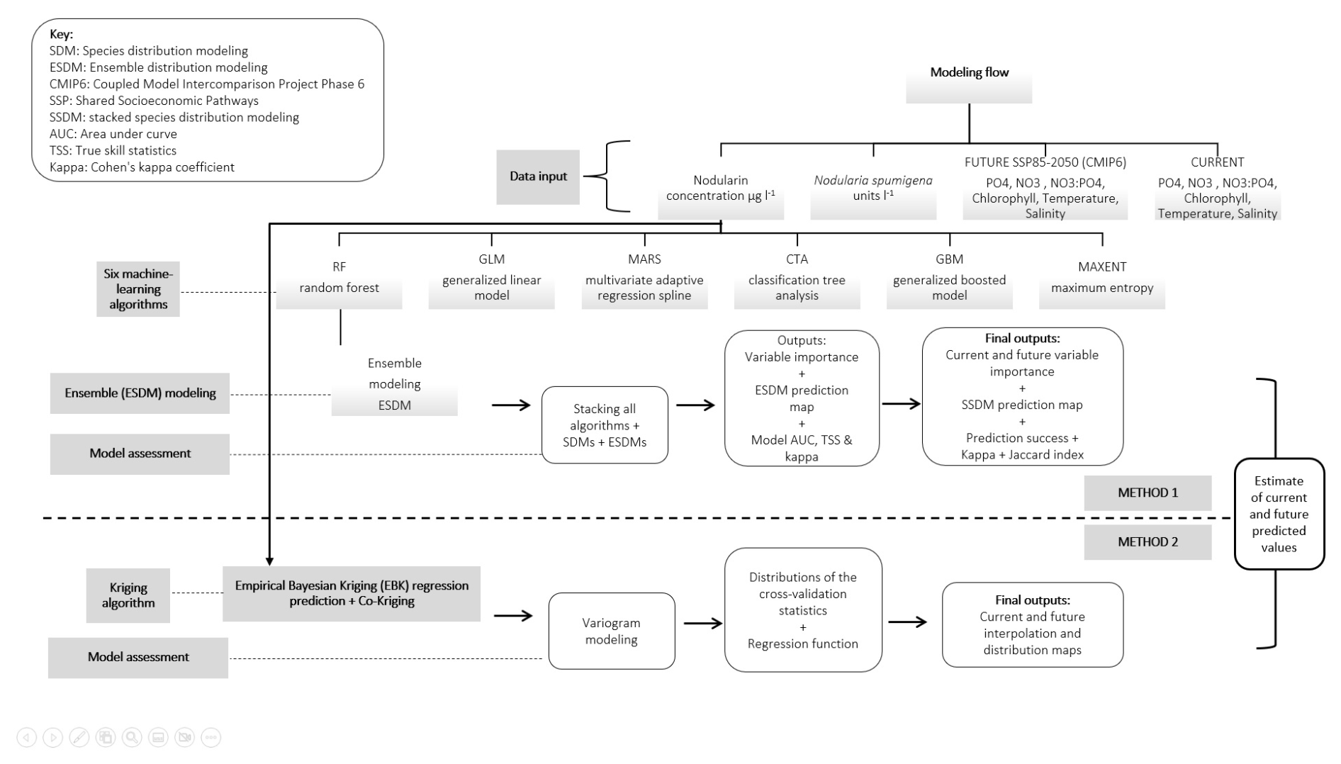
Figure 1 A diagram showing the modeling flow used to predict the present and future spatial occurrence of cyanobacteria and the toxin nodularin in the Baltic Sea.

2.2 Data collection and environmental parameters

Data was compiled for 139 samples in 54 locations across the Baltic Sea, the Kattegat, and the Skagerrak, sampled June to September 2023 (Fig. 2). The dataset comprised locations in longitude and latitude with corresponding nodularin in biomass (µg L⁻¹), collected onto 47 mm GFC filters and analyzed using enzyme-linked immunoassay (ELISA) for microcystins/nodularins from Gold Standard Diagnostics, following the manufacturer's instructions; and the abundance of Nodularia spumigena (units L⁻¹) based on Olenina et al. (2006).

Prediction and geostatistical interpolation of spatial occurrence of nodularin was investigated using different environmental and geographical variables. In this study we used data from samples collected in monitoring programs and results from modelled concentrations of chlorophyll a in surface water (mg m⁻³) from the Baltic Sea Biogeochemistry Analysis and Forecast (ERGOM) (https://doi.org/10.48670/moi-00009) (Neumann et al., 2021). Concentration of inorganic dissolved nutrients: phosphate PO₄, nitrate NO₃ (µmol m⁻³) originate from results of a Baltic Sea Biogeochemistry Reanalysis by SMHI (https://doi.org/10.48670/moi-00012, last access: 16 January 2025). Salinity and sea surface temperature (°C) are based on Global Ocean Physics Analysis and Forecast (https://doi.org/10.48670/moi-00016, last access: 16 January 2025). Salinity was derived from the Baltic Sea Physics Reanalysis by SMHI (https://doi.org/10.48670/moi-00013, last access: 16 January 2025). The data was downloaded from E.U. Copernicus Marine Service Information (European Union-Copernicus Marine Service, 2016, 2018a, b, 2019). Downloaded modelled data with a horizontal resolution of 1 nautical mile (1.852 km) and vertical depth layers varying between 1–24 m were limited to the period of sampling from June to September 2023 at a depth range of 0.5 to 10 m. Data was downloaded as NetCDF-4 format and transformed to ESRI raster grid file format “GeoTIFF” in QGIS Desktop 3.34.13 (QGIS Development Team, 2022).

The model data from Copernicus were compared with data from measurements made in the National Swedish Marine Monitoring Program, including mean values of chlorophyll, NO₃, PO₄, salinity, and temperature, downloaded from the Swedish National Oceanographic Data Centre (NODC) at SMHI (https://shark.smhi.se/hamta-data, last access: 18 March 2025), accessed in March 2025. A comparison of the derived satellite remote sensing data or modelled data and the observations in the monitoring program are presented in the results and supplementary data.

Furthermore, prediction of nodularin concentration and N. spumigena spatial distribution modeling was tested using results from modelled data available at Copernicus, i.e., mean sea surface temperature, chlorophyll, salinity, PO₄, NO₃, distance to shore (m), and future climate change scenarios developed under the Shared Socioeconomic Pathway (SSP) scenarios of future climate change. Data layers reflecting future conditions following the Paris Agreement of reduced greenhouse gas emissions, to the “fossil-fueled development” SSP5-8.5 scenario of high emissions and low challenges to adaptation (Assis et al., 2024). Raster layers were derived from Atmosphere-Ocean General Circulation Model (AOGCM) downscaled dataset as raster grids at 2.5 arc-minute spatial resolution, approximately 5 km² grid cell sizes at the equator corresponding to future greenhouse gas concentrations in the year 2100. To ensure the data integrity and that the model is internally consistent, future climate change scenarios were downloaded with the same high resolution for the current selected variables from all sources (near-surface chlorophyll, nitrate, phosphate, salinity, and temperature). This will ensure that, along with integrity, consistency, and accuracy, the transition from current data to forecasted data (future predictions) is seamless and logical, preventing abrupt, unrealistic shifts in the model's trajectory.

All environmental data and climate change scenarios were downloaded as raster GeoTIFF from Bio-ORACLE project v3.0 (Assis et al., 2024), using “sdmpredictors” package (Bosch and Fernandez, 2022) in RStudio (RStudio Team, 2020). All raster layers were cropped to the spatial extent of the Baltic Sea (latitude/longitude: min 10, max 30/min 53, max 66) and coordinate reference system (CRS) EPSG: 5845-SWEREF99 TM. Environmental data corresponding to each sampling location (XY coordinates) and time point were extracted in RStudio equipped with R v.4.4.0 (R Core Team, 2021) using the function implemented in the packages “raster” (Hijmans and Etten, 2012),“sp” (Bivand et al., 2013; Pebesma and Bivand, 2005) and “tidyverse” (Wickham et al., 2019). Data holding all information in “csv” format was exported to ESRI Shapefile “shp” in QGIS to be used for the analysis.

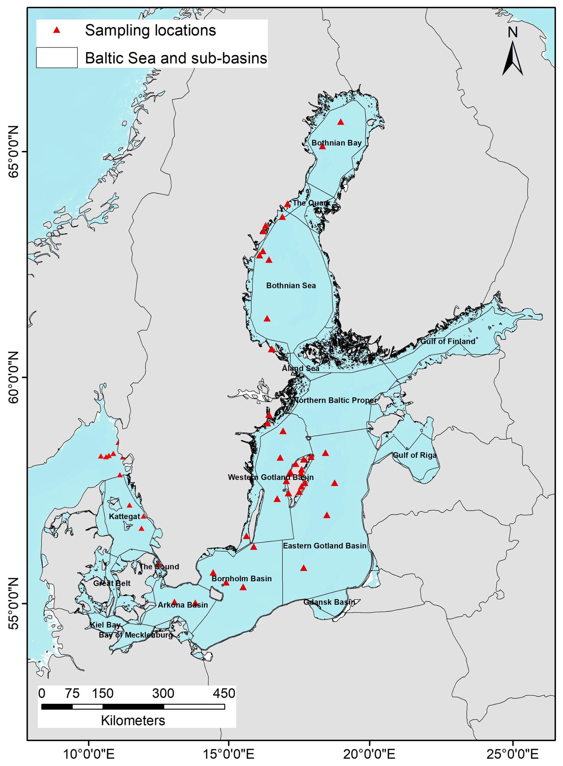
Figure 2 Map of the Baltic Sea indicating sampling locations from where nodularin was analyzed. Sub-basins described in this study are abbreviated on the map as follows: BB = Bothnian Bay, QU = The Quark, BS = Bothnian Sea, ÅS = Åland Sea, NBP = Northern Baltic Proper, WGS = Western Gotland Sea, EGS = Eastern Gotland Sea, BoB = Bornholm Basin, AB = Arkona Basin, and K = Kattegat.

2.3 Test of independency and multicollinearity between predictors

To assess the independency of predictors downloaded from Copernicus and SMHI, a variance inflation factor (VIF) for testing multicollinearity and a correlation matrix analysis based on Pearson correlation coefficient (r) were performed. VIF was assessed under the assumption that if VIF < 5: low multicollinearity, 5 ≤ VIF ≤ 10: moderate multicollinearity, and if VIF > 10: high multicollinearity. Furthermore, tests for independency were also performed in two-dimensional principal component analysis (PCA).

2.4 Geostatistical interpolation analysis

Analysis and prediction of nodularin occurrence was performed using the Empirical Bayesian Kriging (EBK) Regression Prediction based on Gaussian process regression (see Oliver and Webster, 1990). The cross-validation method “leave-one-out resampling” was used to examine how interpolation model fits the data (Dubrule, 1983; Zhang and Wang, 2010). In brief, regression prediction was performed using nodularin concentration as dependent variable and the environmental variables (in raster format) as independent. The EBK regression predictions were validated using 1000 simulations as cross-validation. Prediction for nodularin occurrence in response to N. spumigena abundance was performed using CoKriging (Goovaerts, 1997, 1998). Furthermore, spatial interpolation of nodularin in response to the mean values measured by National Swedish Marine Monitoring to was performed using co-kriging by applying nearest neighbor as proximal interpolation method. Geostatistical interpolation analysis was performed in QGIS and by Esri. ArcGIS^® and ArcMap™.

2.5 Ensemble prediction of nodularin occurrence and Nodularia spumigena distribution

Prediction for current and future occurrence of nodularin was performed using Ensemble learning method (Araújo and New, 2007), and modeling occurrence of N. spumigena performed using Stacked Species Distribution Modeling SSDM (Schmitt et al., 2017). Models were built using six different machine-learning algorithms including Classification Tree Analysis CTA (Steinberg, 2009), Maximum-Entropy learning MAXENT (Phillips et al., 2006), Multivariate Adaptive Regression Spline MARS (Friedman, 1991), Random Forest RF (Breiman, 2001), Generalized Boosting regression Model GBM (Friedman, 2002), and Generalized Linear Model GLM (Guisan et al., 2002).

In brief, models were built by creating two data objects with the `sdmData' function in the “sdm” package (Dietterich, 2000; Naimi and Araújo, 2016). The first data object for nodularin ensemble prediction was created by having the occurrence as presence “1” and absence “0”, measured concentrations and all environmental variables. Second data object for the species ensemble and stacked distribution modeling was created by having all occurrence records of N. spumigena, environmental variables, and 10 000 pseudoabsence datapoints randomly generated within the spatial extent of the study area as a background (Barbet-Massin et al., 2012). The two prediction models were tested with 10-fold bootstrapping (Harrell et al., 2005; Lima et al., 2019) as the replication technique and validated in a repeated split-samples procedure, i.e., 70 % of the occurrence dataset was used for model training and the remaining 30 % as test data repeated over 10-fold cross validation (Roberts et al., 2017).

Models were assessed for prediction success, omission rate (Franklin, 2010; Phillips et al., 2006), accuracy and performance based on Area Under the Curve AUC (Hanley and McNeil, 1982), True Skill Statistics TSS (Monserud and Leemans, 1992), Cohen's KAPPA coefficient (Allouche et al., 2006), and Jaccard coefficient (Jaccard, 1912). Predicted variables of importance and percentage of contribution were assessed using AUC, Pearson Correlation coefficient (Benesty et al., 2009) and Jackknife test (Efron, 1982).

2.6 Statistical analysis

The effect of both environmental variables and abundance of N. spumigena on the predicted nodularin concentrations were quantified using Bayesian linear regression (see Clyde et al., 2011), ANOVA and GLM. The effect and interaction effects between predictors on nodularin concentration were assessed using Bayes factor BF₁₀, p-value (at p<0.05), coefficient of determination R² and Pearson correlation coefficient. Assessment of the EBK regression prediction models was performed using cross-validation statistics with a regression function calculated using a robust regression procedure. Variable contributions on nodularin concentration were visualized in the linear two-dimensional space of principle component analysis (PCA). Ordination and visualization were performed using the “FactoMinR” package (Lê et al., 2008) in RStudio (RStudio Team, 2020). To assess relative importance of predictors, the LMG metric (Lindeman et al., 1980) for variance-decomposition measure was calculated using the package “relaimpo” (Grömping, 2006). Statistical analyses were performed in RStudio, and open software jamovi v.2.3.21 (The jamovi project, 2023) and JASP v.0.19.3 (JASP Team, 2025).

3 Results

3.1 Test of independency and multicollinearity between predictors

Tests of multicollinearity show that all VIFs were below the common threshold of 5, showing that there is no indication of severe multicollinearity in Copernicus and SMHI predictors (Fig. S8a, b). Test of pairwise correlation show that salinity, PO₄ and temperature had highest positive correlation (r ≈ 0.6–0.7). Salinity correlation with temperature reflecting seasonal temperature–salinity structure which could be driven by atmospheric conditions, runoff, and water density properties, while PO₄ correlation with temperature typically reflects that higher temperatures accelerate internal phosphorus loading from sediments (Mallissery et al., 2025; Stockmayer and Lehmann, 2023; Walve et al., 2018). On the other hand, all pairwise correlations are typically low ($\left|r\right|\mathit{<}\mathrm{0.3}$), indicating that most variable-pairs vary independently (Fig. S8a, b).

3.2 Results of geostatistical interpolation analysis

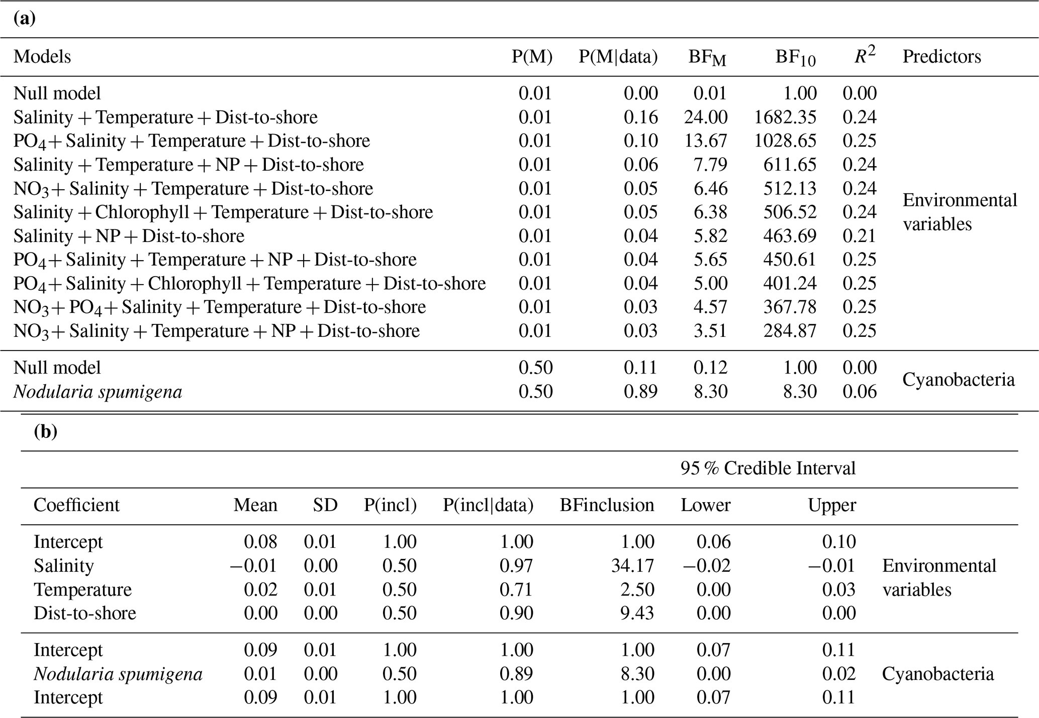
Prediction of nodularin spatial occurrence was first tested using environmental predictors from the European Copernicus dataset of Baltic Sea Biogeochemistry Analysis and Forecast (ERGOM). Results of the Bayesian linear regression show that there were significant interaction effects between concentrations of salinity, temperature, and distance to shore (BF₁₀>1, R²=0.23, regression function: $\mathrm{0.70}\times x+\mathrm{0.004}$), and between PO₄, salinity, temperature, and distance to shore (BF₁₀>1, R²=0.23, regression function: $\mathrm{0.70}\times x+\mathrm{0.008}$) and the abundance of Nodularia spumigena (BF₁₀>1, R²=0.1) on predicted spatial occurrence of nodularin (Tables 1a, b, S1, Fig. 3). This finding is also supported by the regression function of the EBK regression prediction (distance to shore: $\mathrm{0.74}\times x+\mathrm{0.001}$; salinity: $\mathrm{0.73}\times x+\mathrm{0.003}$; temperature: 0.76×x + 0.003), see Figs. 4, S1. Analysis of ordinary and multiple linear regression shows that there was significant positive linear regression of temperature, and distance to shore (p<0.05), and negative with salinity (p<0.001), (linear regression R²=0.3, multiple R²=0.2). Analysis of variance ANOVA shows that there was significant effect of salinity (ANOVA, F=11.11, p<0.001), PO₄ (ANOVA, F=6.6, p<0.01), NO₃ : PO₄ ratio (ANOVA, F=5.03, p<0.05), distance to shore (ANOVA, F=4.73, p<0.05), temperature (ANOVA, F=3.93, p<0.05) with interaction effects between chlorophyll, temperature (ANOVA, F=7.27, p<0.01), NO₃, temperature (ANOVA, F=6.70, p<0.05), and between chlorophyll and distance-to-shore (ANOVA, F=4.59, p<0.05), Fig. 3, Tables S2, S3a, S3b. These findings can also be described by exploring the variogram and nugget analysis provided in Fig. S2.

Table 1 First panel (a) shows the best 10 models for Bayesian linear regression analysis between nodularin concentration as dependent and environmental variables and Nodularia spumigena abundances as predictors, and second panel (b) posterior summaries of coefficients. The Bayes factor BF₁₀ is a ratio which quantifies evidence in favor of an effect (represented by “1”) versus no effect (represented by “0”). If BF₁₀>1 indicates evidence in favor of an effect. 0< BF₁₀<1 indicates evidence in favor of no effect. The P(M) indicates that the prior probabilities of the other models are equal, P(M|data) refers to the posterior probability of each model after seeing the data while BF_M compares each model to the average P(M|data) of the other models. For all Bayesian linear regression models and effects refer to Table S1.

Geostatistical interpolation based on the interaction effects between predictors indicated area increases of nodularin into the Eastern Gotland Sea, Northern Baltic Proper, Bornholm and Arkona basin (Fig. 3a, b, c, e), and Western Gotland Sea Fig. 3a, b as result of interactions between salinity, temperature, distance to shore, PO₄, and chlorophyll. There is an area increase of nodularin into the Bothnian Sea in response to interaction between salinity, temperature, and chlorophyll with distance to shore (Fig. 3a, e). The northern parts of the Baltic Sea at Bothnian Bay and southern parts at Kattegat predicted low or no increase in nodularin.

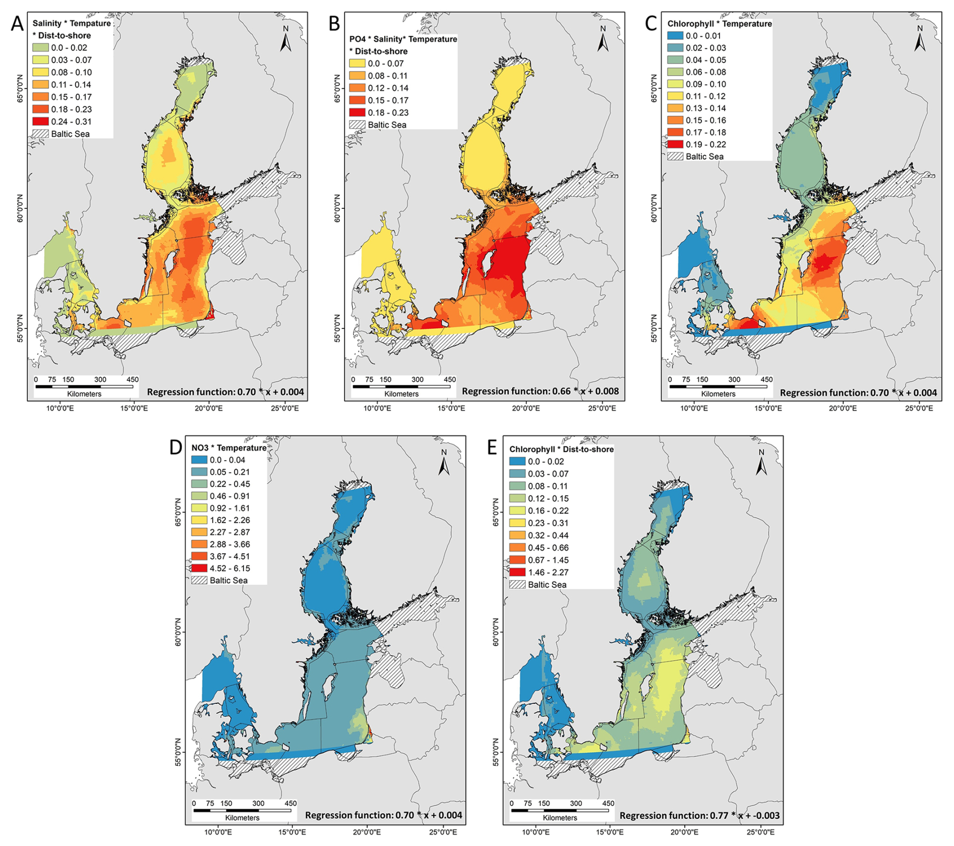
Figure 3 Empirical Bayesian kriging (EBK) regression prediction of the model-predicted concentration and area distribution of nodularin (µg L⁻¹) at different sampling sites across the Baltic Sea. Predicted area distribution and concentrations of nodularin are based on the coefficient of determination R² of Bayesian linear regression in (Table S1) and significant interaction effects of ANOVA at p<0.05 (Table S3) between (a) salinity, temperature and distance to shore (b) PO₄, salinity, temperature and distance to shore (c) chlorophyll and temperature, (d) NO₃ and temperature and between (e) chlorophyll and distance to shore. The regression function of kriging describes the relationship between nodularin concentration and interaction effect between independence variables. Grading colors in key legend corresponds to predicted concentrations of nodularin (µg L⁻¹). Significant interaction effects in (a) and (b) were quantified using Bayesian linear regression while (c), (d) and (e) were assessed in ANOVA. Geostatistical interpolations are performed using nodularin concentration as dependent variable and environmental variables in raster GeoTIFF format as independents. Environmental data was retrieved from E.U. Copernicus Marine Service Information during the period of sampling from June to September 2023 at a depth range of 0.5 to 10 m.

Predicted area distribution show increases of nodularin occurrence in Eastern Gotland Sea and Northern Baltic Proper in response to PO₄, salinity temperature, and distance to shore (Fig. 4c, e, f, g); and in Bothnian Sea and Åland Sea in response to Chlorophyll, NO₃ : PO₄ ratio, and temperature (Fig. 4a, d, f). There are increases in area distribution of nodularin in Arkona Basin and Bornholm Basin in response to chlorophyll, PO₄, salinity, NO₃ : PO₄ ratio, temperature and distance to shore (Fig. 4a, c, d, e, f, g). Despite measured occurrences of nodularin, Kattegat and some parts of the Bothnian bay are predicted to have no or low area distribution of nodularin.

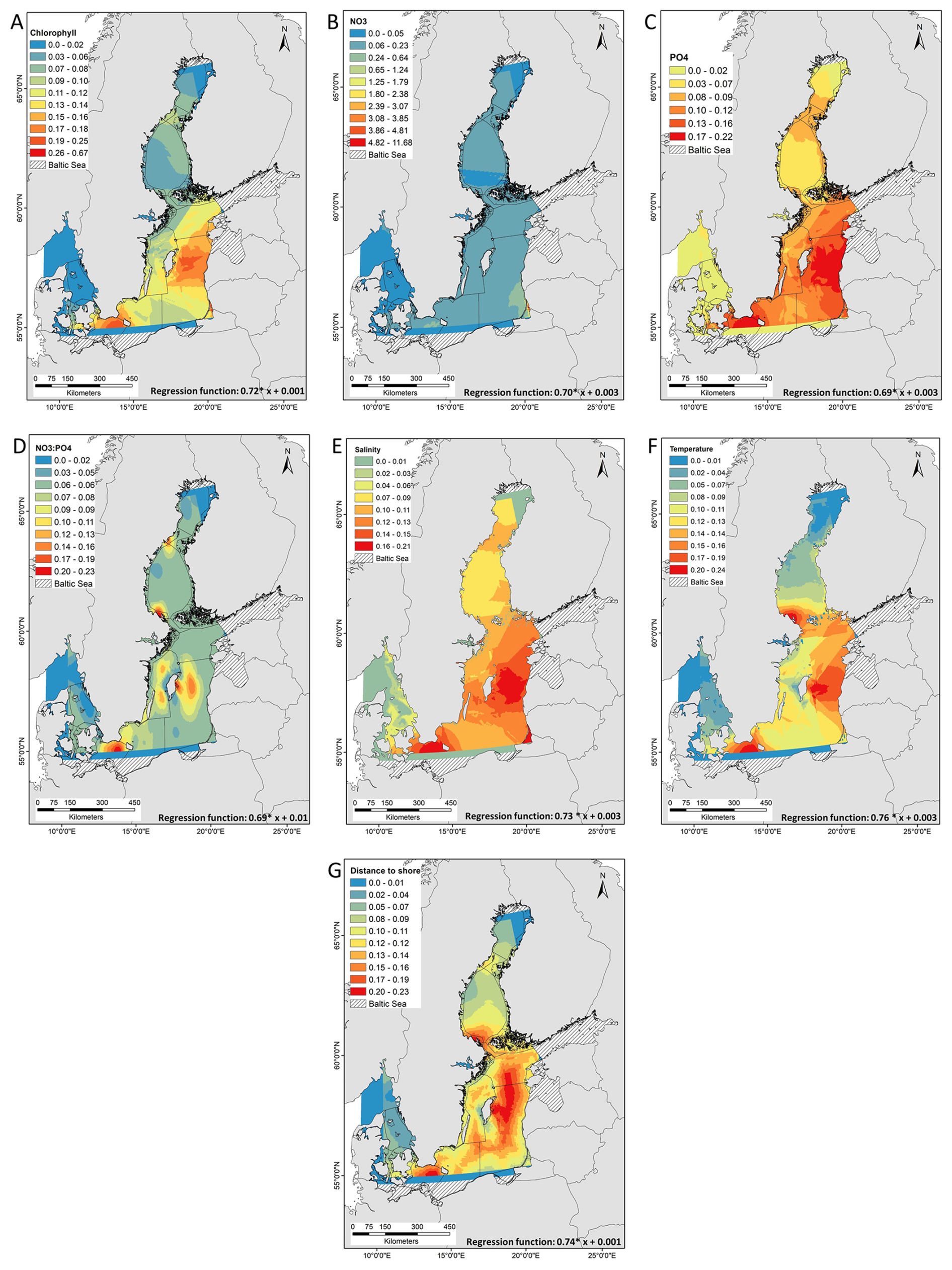
Figure 4 Empirical Bayesian kriging (EBK) regression and co-kriging prediction of the model-predicted concentration and area distribution of nodularin (µg L⁻¹) at different sampling sites across the Baltic Sea. Predicted area distribution and concentrations of nodularin are based on sea surface concentrations of (a) chlorophyll mg m⁻³ (b) nitrate NO₃ µmole m⁻³, (c) phosphate PO₄ µmole m⁻³, (d) NO₃ : PO₄ ratio, EUR salinity, (f) temperature ° and (g) distance to shore (m). The regression function of kriging describes the relationship between nodularin concentration and each independent variable. Grading colors in key legend corresponds to predicted concentrations of nodularin (µg L⁻¹). Geostatistical interpolations are performed using nodularin concentration as dependent variable and environmental variables in raster GeoTIFF format as independents. Environmental data was retrieved from E.U. Copernicus Marine Service Information during the period of sampling from June to September 2023 at a depth range of 0.5 to 10 m.

There was a conformity in area distribution of nodularin in response to measured abundances of N. spumigena (Fig. 5). Predicted area distribution shows a slight increase in nodularin occurrence into Western Gotland Sea, Eastern Gotland Sea, Arkona Basin and in southern and northern parts of Bothnian Sea. Predicted area distribution of nodularin was significantly driven by abundances of N. spumigena (ANOVA, F=8.51, p<0.001, BF₁₀>1, R²=0.1) see Tables 1, S3b. Predicted area distribution in response to measured abundances of N. spumigena show increases in occurrence of nodularin into Northern Baltic Proper and Eastern Gotland Sea, see Fig. 5 and regression function.

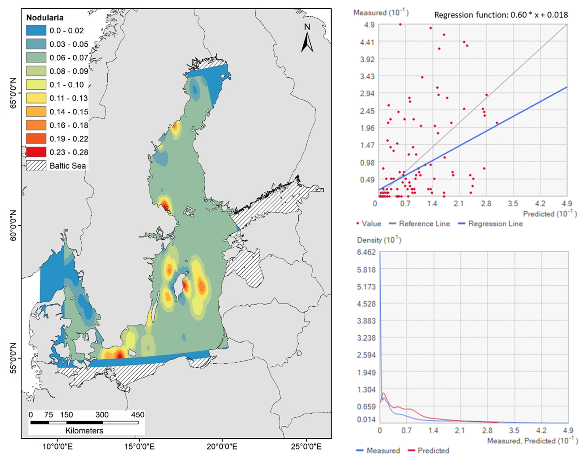
Figure 5 Spatial prediction map of Co-kriging interpolation (left) and distributions of the cross-validation statistics (right), estimated using kernel density, show the prediction regression scatterplot, the regression function of the concentration and predicted area distribution of nodularin (µg L⁻¹) at different sampling sites across the Baltic Sea. Grading colors in key legend corresponds to predicted concentrations of nodularin (µg L⁻¹). The blue and red lines correspond to the measured and predicted values of nodularin (µg L⁻¹). Predicted area distribution and concentrations of nodularin are based on the measured abundances of Nodularia spumigena.

Prediction and geostatistical interpolation of nodularin based on measured mean values obtained from Swedish National Oceanographic Data Centre (NODC) at SMHI shows that there were significant interaction effects between temperature and distance-to-shore and between salinity, PO₄, temperature and distance-to-shore on predicted spatial occurrence of nodularin (BF₁₀>1, R²=0.1), Table S4. Prediction of occurrence of nodularin based on mean values measured by Swedish National Oceanographic Data Centre (NODC) showed that they are occurring at the Eastern and Western Gotland Sea, Northern Baltic Proper, Bothnian Sea, The Quark and Arkona basin. Predicted area distribution of nodularin based on NODC values showed similar distribution patterns as the prediction made with full location dataset using Copernicus values (see Fig. S3).

Future predictions of nodularin occurrence based on projected climate change scenarios (SSP5-8.5) in year 2100 show that there are areas increases of occurrence into the Eastern Gotland Sea, Northern Baltic Proper, the Bothnian Sea, the Quark, and Arkona Basin in response to chlorophyll, NO₃, PO₄, salinity and temperature (regression function: $\mathrm{0.73}\times x+\mathrm{0.005}$), Fig. 6. Bayesian linear regression shows that there is area increase of nodularin in response to NO₃ (ANOVA, F=25.33, p<0.0001, BF₁₀>1, R²=0.25), Fig. S4, Table S5a. There was a significant linear regression revealed by multiple linear regression (Multiple R=0.5, Multiple R²=0.2, 95 % CI [5, 127]) with negative coefficient observed in NO₃ (p<0.05), see Table S5b.

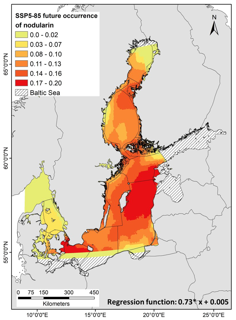
Figure 6 Empirical Bayesian kriging (EBK) regression prediction of the model-predicted concentration and area distribution of nodularin (µg L⁻¹) (estimated using kernel density) show area distribution and regression function of the concentration predicted at different sampling sites across the Baltic Sea. Grading colors in key legend corresponds to predicted concentrations of nodularin (µg L⁻¹). Predicted area distributions are based on projected future concentrations of chlorophyll, NO₃, PO₄, salinity and temperature. Predicted area distribution and concentrations of nodularin are based on Shared Socioeconomic Pathway (SSP5-8.5) scenarios of future climate change corresponding to future greenhouse gas concentrations in the year 2100. Climate change scenarios were downloaded as raster GeoTIFF from Bio-ORACLE project v3.0. Geostatistical interpolations are performed using nodularin concentration as dependent variables and SSP5-8.5 variables in raster GeoTIFF format as independents. Models are validated using 1000 simulations as cross-validation.

3.3 Ensemble prediction of nodularin occurrence and Nodularia spumigena distribution

After removing collinear environmental layers with Pearson correlation coefficient ≥ 0.7, that is NO₃ : PO₄, six predictors were used in the ensemble modeling. Since we applied pseudoabsence points as background, data points in areas predicted by Kriging with no nodularin occurrence, particularly on the Swedish west coast, were removed from the ensemble modeling to avoid overestimation. The overall ensemble model performance was excellent (Current: Threshold = 0.35, AUC = 0.84, proportion of correct prediction = 0.72; Future: Threshold = 0.40, AUC = 0.80, proportion of correct prediction = 0.71), see Table S6. The average performance of the six algorithms was excellent (Current: AUC = 0.75±0.05, TSS = 0.48±0.11; Future: AUC = 0.77±0.07, TSS = 0.52±0.12), in which RF, GBM, MAXENT, GLM and MARS had highest AUC values (between 0.73–0.87) indicating excellent performance, Fig. S5. Response curves of ensemble learning modeling illustrating the effects of the predicted variables and projected climate change scenarios on nodularin occurrence can be found in Fig. S6.

Variables predicted with highest contribution to current nodularin occurrence were NO₃ (AUC = 0.2, Pearson coefficient = 0.4), temperature (AUC = 0.1, Pearson coefficient = 0.4), distance to shore (AUC = 0.1, Pearson coefficient = 0.4), PO₄ (AUC = 0.1, Pearson coefficient = 0.3), and salinity (AUC = 0.1, Pearson coefficient = 0.2), see bar chart in Fig. 7a. Predicted climate change scenarios with highest contribution were NO₃ (AUC = 0.2, Pearson coefficient = 0.4), salinity (AUC = 0.1, Pearson coefficient = 0.3), and temperature (AUC = 0.1, Pearson coefficient = 0.3), see bar chart in Fig. 7b.

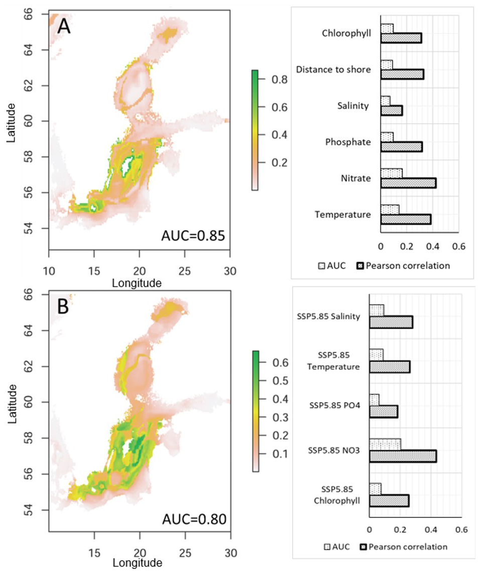
Figure 7 Binary maps show the ensemble learning prediction for nodularin occurrence in response to (a) current environmental variables and (b) future climate change scenarios SSP5-8.5 in 2100. The bar charts show variable contributions to predicted distribution as revealed by the ensemble model. The scale bar from 0.1–0.8 shows predicted suitable areas where dark green colors correspond to areas predicted to have high nodularin occurrence. Models are assessed using area under curve AUC and Pearson correlation coefficient. AUC values close to 1.0 indicate excellent model performance.

There was conformity in predicted area distribution of nodularin between ensemble learning and EBK regression prediction method. There is an increase in nodularin occurrence predicted into the Eastern Gotland Sea, Arkona Basin and Kattegat in response to the six environmental variables (Figs. 6a and 7a). Area increases of nodularin occurrence in response to future scenarios in 2100 are predicted into the Eastern, Western Gotland Sea, Northern Baltic Proper, Arkona Basin, Kattegat and southern parts of Bothnian Bay in the Quark area Figs. 6b and 7b.

There is also a conformity in the predicted area increase of nodularin and predicted distribution for N. spumigena. Predicted areas revealed by SSDM are the coastal sites along the Eastern Gotland Sea, and Northern Baltic Proper, along with Western Gotland Sea, Arkona Basin and Kattegat (Kappa = 1.0±0.23), Fig. 8a. Predicted area distribution of N. spumigena in response to future climate change scenarios are Eastern, Western Gotland Sea, Northern Baltic Proper, Arkona Basin, Kattegat and southern parts of Bothnian Bay in the Quark area (Kappa = 1.0±0.16), Fig. 8b.

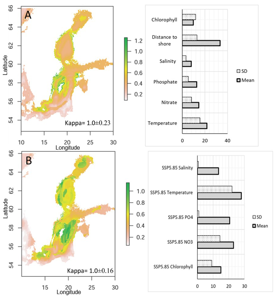
Figure 8 Binary maps show the predicted distribution of Nodularia spumigena estimated by stacked species distribution modeling SSDM in response to (a) current environmental variables and (b) projected climate change scenarios SSP5-8.5 in the year 2100. The bar charts show variable contributions to predicted distribution as revealed by SSDM in Mean ± SD. The scale bar from 0.2–1.2 unit represents the degree of suitability in which warmer colors correspond to highly predicted suitable areas. Model performances are assessed using Cohen's kappa as Mean ± SD, in which Kappa values close to 1.0 indicate excellent model performance.

3.4 Relative contribution of predictors to nodularin concentration

Variable contribution to nodularin concentration as measured by LMG method shows that abundance of N. spumigena had largest positive effect (with ERGOM: p=0.0003, LMG % = 20.0; with NODC: p<0.05, LMG % = 28.5) followed by salinity (with ERGOM: p<0.001, LMG % = 15.2; with NODC: p = 0.01, LMG % = 24.0), see Fig. S7 and Table S7 for the rest effects of predictors. The coefficient of determination R² of both models, as calculated using LMG method, indicates the total proportion of variance in nodularin explained by all eight predictors jointly (ERGOM: R²=0.78, NODC: R²=0.72).

4 Discussion

Blooms of toxic cyanobacteria are a global issue, and it's challenging to make predictions of toxin occurrence as the connection to organism abundance is not straightforward (Huisman et al., 2018; Ibelings et al., 2021). Therefore, understanding bloom formation and toxicity of cyanobacterial blooms in the Baltic Sea is difficult using observational data alone. Here, models can be very effective in increasing spatial and temporal resolution and the interconnection between abundance and toxicity. As a proof of concept, we integrated and compared the results of two different modeling approaches to understand and interpret the current and future spatial expansion of nodularin occurrence across the Baltic Sea. Although there are no expectations on substantial variations in degree of accuracy between geostatistical and ML-based predictions, there has in recent years been a general move from geostatistics to machine learning (Veronesi and Schillaci, 2019). According to the same study, the number of documents mentioning ML algorithms-based predictions has rapidly increased, surpassing kriging-based algorithms in the last decade. Our findings suggest the efficiency of both kriging and ML algorithms given that the overall geographical estimations and maps produced by the kriging and ensemble-based models in this study are aligned despite the differences of approaches. Findings suggest that the model generated by the integrated method is yielded by using advantages of both methods, which in turn increase prediction accuracy and performance.

Several abiotic variables, such as PO₄, NO₃, sea surface temperature, and salinity, are known to directly or indirectly affect and control the abundance of cyanobacteria (Almroth-Rosell et al., 2016; Andersen et al., 2020; Karlson et al., 2010; Lips and Lips, 2008; Lu et al., 2019; Olofsson et al., 2020a; Stal, 2009; Unger et al., 2013; Wurtsbaugh et al., 2019; Yang et al., 2008), and therefore we also included many environmental factors. Considering the importance of abiotic variables in modeling cyanobacterial abundance, the corresponding general ocean circulation models GCMs require adequate horizontal and vertical resolution and trustworthy boundary conditions. An earlier study by Reissmann et al. (2009) showed that variations in GCMs are likely to affect the simulation of cyanobacteria (see also Munkes et al., 2021). Therefore, we employed different GCMs to reduce possible errors that could arise from abiotic variables of different ocean models. Our simulation showed that there were conformities in predicted distribution of nodularin despite the different GCMs used in this study. Although each one of the combined approaches has different working procedures, each model effectively yielded similar performance observed in the predicted distribution of nodularin occurrence across the Baltic Sea. This finding indicates that both kriging and ML-based algorithms, the ensemble, can capture the differences in abiotic variables of different GCMs. The findings also suggest that the approach could help resolve the error arising from great divergence between general circulation models (GCMs) when used for predicting the presence or occurrence of cyanotoxins.

Using our conceptual model-setup we were able to locate areas with high predicted nodularin concentrations in response to current environmental variables and projected future changes of the same variables. These areas were the Eastern and Western Gotland Sea, the Northern Baltic Proper, southern parts of the Bothnian Sea, and the Arkona basin, corresponding to the effects and interactions between temperature, PO₄, NO₃ : PO₄, salinity, and distance to shore. The effects of temperature, PO₄ and NO₃ : PO₄ are aligned with previous studies by Deng et al. (2022); Lürling et al. (2017), and Olofsson et al. (2016), documenting that water temperature increase is associated with higher nutrient loads and phosphate release from sediments, all of which could have an impact on cyanobacterial biomass increase. Rising temperature is also associated with terrestrial runoff of organic matter but also causes a decrease in salinity in the northern Baltic Proper, northern parts of the Bothnian Sea, Bothnian Bay, and southward to the Arkona basin (see Andersson et al., 2013, 2015). Moreover, the increase in the abundance of cyanobacteria may also be associated with basin-specific decreases in salinity (Kuosa et al., 2017; Olofsson et al., 2020a; Suikkanen et al., 2007), which could highlight the area increase of nodularin predicted in the Arkona basin.

To further investigate whether nodularin accumulates closer to or far from the shoreline, we included the geographical variable “distance to shore” as a predictor. Results of Bayesian regression show that distance to shore, surprisingly, appears to have significant positive direct and interaction effects together with other variables on the predicted area increase of nodularin. Our findings show that predicted sites with high nodularin concentration are located further offshore. Considering the differences in biogeochemical characteristics between coastal and offshore waters (Vigouroux et al., 2021) and that offshore waters are generally more nutrient-depleted than waters closer to the coast (see Löptien and Dietze, 2022), our results, in contrast to common assumption, suggest that predicted occurrence of nodularin is not only driven by nutrient concentrations like PO₄ and NO₃. However, the predicted occurrence of nodularin in nutrient-depleted areas could be attributed to the limitation of model-based projection of nutrient load scenarios, which do not differentiate between dissolved inorganic phosphorus stored by cyanobacteria and dissolved organic phosphorus. The fact that cyanobacteria can utilize dissolved organic phosphorus under nutrient-depleted conditions (see Caille et al., 2024; Rabouille et al., 2022) could explain the observed and predicted occurrence of nodularin. Our model finding suggests the importance of including distance to shore as a geographical variable in future modeling of cyanobacteria and cyanotoxin, particularly in nutrient-depleted areas across the Baltic Sea.

To explore what drives predicted area distribution of nodularin, we analyzed the interaction effect of the selected predictors. Results of Bayesian linear regression show that there were variations in the interaction effects between different variables of ERGOM and NODC on the predicted occurrence of nodularin, with a relatively low coefficient of determination R²≤0.25. This statistical observation can be attributed to the differences in resolutions of variables measured by GCM of different origins (see e.g., Dietze and Löptien, 2016; Löptien and Dietze, 2022; Meier et al., 2011; Meier and Kauker, 2003; Munkes et al., 2021; Schrum and Backhaus, 2002). However, these statistical observations are not great enough to offset the spatial regression observed in the regression function R²≥0.7 and the detrimental and significant effects of other variables with p<0.001, 0.01 and 0.05 observed, e.g., in salinity, temperature, PO₄, distance to shore, and their interaction effects. Despite the statistical results of Bayesian linear regression, our model finding suggests that the spatial regression function produced by the kriging algorithm is useful to interpret the drivers of the predicted occurrences of nodularin.

Future increased occurrence of nodularin was predicted for the Eastern Gotland Sea, Northern Baltic Proper, the Bothnian Sea, the Quark, and Arkona Basin in response to overall projected changes in environmental variables, particularly the NO₃ concentration and temperature. Earlier studies demonstrated that cyanobacterial taxa, such as Nodularia spumigena and Aphanizomenon spp., will benefit from climate change due to increased stratification by higher temperatures and that the growth and nitrogen fixation are favored by rising temperatures (Karlberg and Wulff, 2013; Munkes et al., 2021; Paerl and Otten, 2013; Visser et al., 2016). Furthermore, it has been shown that the effects of climate change under different scenarios are smaller than the effects of considered nutrient load changes (Saraiva et al., 2019). Taken together, our model findings suggest that reducing nutrient load could lead to improved future environmental conditions in the Baltic Sea, which in turn could reduce future area distribution of nodularin.

Results of the LMG based on ERGOM and NODC data, where N. spumigena leads the importance ranking is biologically intuitive: toxin concentration is closely tied to the abundance of the toxin-producing organism itself. Contribution of salinity (15.2, 24 %) and chlorophyll a (12.8, 12 %) indicate that both ionic conditions and overall phytoplankton biomass modulate nodularin concentrations. Nutrient availability (NO₃, PO₄ and N : P jointly contribute ∼ 24.2 %) is the next most influential factor especially NO₃, all reflecting that N supply often governs cyanobacterial growth and secondary metabolite production. Temperature (18.5, 10 %) is environmental modulator that further tunes metabolic rates and community composition. Furthermore, distance to shore (9.3, 1.0 %) as proximity to the shore possibly reflects nutrient loading or mixing regimes, which in turn affect nodularin levels. These findings suggest that while biological factors (Nodularia abundance and chlorophyll) and temperature are dominant, both physicochemical conditions (salinity, nutrients, and distance to shore) play appreciable roles in explaining variation in nodularin. The two full models explain about 78 % and 72 % of the total variance in nodularin, suggesting that more variables can be included to further reveal conditions under which toxin-producing blooms thrive.

Given the great divergence and large spread between findings of other models projecting cyanobacterial bloom (e.g., Hense et al., 2013; Meier et al., 2012, 2019; Munkes et al., 2021; Neumann, 2010; Saraiva et al., 2019), the variation in GCMs, and that cyanotoxins cannot be directly measured by satellite and remote sensing, our modeling approach that combines geostatistical and ML algorithms could help mitigate this methodological gap. The approach used here shows that while geostatistical methods were able to analyze small spatially correlated datasets to predict values at unsampled locations, the ML algorithms were able to handle complex and non-linear relationships in data that geostatistical models might miss. Model prediction of both EBK regression and ensemble learning provided useful and conformable spatial estimation of nodularin occurrence, suggesting that combining results of geostatistical interpolation and ML-based modeling could serve as a promising future approach for cyanotoxin investigation. Both models, for example, can use the advantages of both techniques to produce predictions that are more accurate than those made by any one model alone. This approach could also help mitigate future expansion of nodularin by detecting and predicting possible hotspot occurrences that could arise due to different future climatic scenarios across the Baltic Sea. Despite the model's accuracy and performance, care should be taken when interpreting the model findings, given that there was limited data availability that covers both nodularin concentration and abundance of N. spumigena in corresponding samples and that the sampling period of the study was conducted only during the summer and in one year. The risk of overfitting due to data limitations is still very high, regardless of using ensemble and model accuracy observed in this study. Although the study integrates different downscaled datasets from global and regional models, a careful inspection should be given to harmonize the datasets, calibrate regional projections using global boundary conditions, align the differing resolutions, and quantify uncertainty. It is also worth mentioning that, despite many efforts made, predicting Nodularia sp. blooms from the environmental factors remains challenging (Kahru et al., 2020; Karlson et al., 2010). Moreover, the integrated model must be carefully inspected to ensure that it is still interpretable and computationally practical, providing that model success and performance are strongly reliant on the quality of the input data.

5 Conclusions

Our proof-of-concept model combination setup used herein demonstrates the need to integrate geostatistical interpolation and machine-learning-based modeling to monitor and mitigate spatial expansion of nodularin across the Baltic Sea and to enhance decision-making strategies in this area. Improved model accuracy using combined approaches may enable more precise recommendations that could help mitigate future expansion of cyanotoxins in the Baltic Sea. Our model combination can be a useful tool to generate spatial estimates of nodularin occurrence at unsampled locations and temporal occurrence when sampling efforts are challenging. We show evidence that the predicted area distribution of nodularin is a result of several interacting environmental variables together with a geographical factor of distance to shore that could further help explain increased expansion into different areas in the future, which is also beneficial from a management perspective. Furthermore, the combined approaches presented in this study could be crucial for effective management applied for nutrient reduction and predicting future climate change impacts, as cyanobacteria can exacerbate eutrophication, affect water quality, and pose health risks. If used carefully, these approaches could help prioritize surveillance and implement earlier sampling efforts in areas predicted to have high and/or increasing cyanotoxin concentration.