A cross-site comparison of ecosystem- and plot-scale methane fluxes across multiple timescales

Wetland and upland ecosystems play significant but opposing roles in the global methane (CH₄) budget, acting as natural sources and sinks, respectively. Two of the most common approaches for measuring CH₄ fluxes (FCH₄) are chambers, which measure fluxes at fine spatial scales (ca. 1 m²), and eddy covariance (EC) towers, which integrate fluxes across larger footprints (ca. 100–10 000 m²). Although chamber and EC observations have been combined in various syntheses and databases to estimate CH₄ budgets, a unified cross-site evaluation of FCH₄ estimates at plot and ecosystem scales is lacking. As a first step toward a systematic spatiotemporal scaling of EC tower and chamber footprints, we quantified differences in site-level aggregate FCH₄ between EC and chamber measurements (ΔFCH₄) across ten wetland and upland sites at half-hourly, hourly, daily, weekly, monthly, and annual timescales. We found that ecosystem-scale median FCH₄ was consistently higher than plot-scale FCH₄ at all temporal scales, with the smallest difference at the daily timescale (multi-site median ΔFCH₄: 1.36 nmol m⁻² s⁻¹; median ecosystem-scale FCH₄ = 1.56 nmol m⁻² s⁻¹, median plot-scale FCH₄ = 0.06 nmol m⁻² s⁻¹) and the largest at annual scales (2.58 nmol m⁻² s⁻¹; median ecosystem-scale FCH₄ = 25.91 nmol m⁻² s⁻¹, median plot-scale FCH₄ = 6.55 nmol m⁻² s⁻¹). In general, the agreement between ecosystem- and plot-scale FCH₄ decreased with finer temporal resolution (from Spearman ρ = 0.95 at the annual scale to ρ = 0.65 at the half-hourly scale), while ΔFCH₄ variation was greatest at daily-to-annual scales. Key environmental predictors of ΔFCH₄ across the ten sites included plot-scale spatial heterogeneity, dominant vegetation type, vapor pressure deficit, atmospheric pressure, and friction velocity at the daily and monthly scales. Wind direction was a significant predictor only at the monthly scale, suggesting EC footprint effects at these sites. These findings suggest that accounting for variability in EC footprint extent, chamber measurement placement, and measurement artifacts is key to reconciling multi-scale FCH₄ observations across diverse ecosystems and refining CH₄ budgets.

1 Introduction

Methane (CH₄), a potent greenhouse gas, is produced in wetlands and consumed in upland soils- respectively the largest natural CH₄ sources and sinks globally. However, the magnitude of these fluxes remains highly uncertain (IPCC, 2023; Saunois et al., 2025). Field measurements of CH₄ fluxes (FCH₄) are often conducted using enclosed chamber systems or eddy covariance (EC) towers (Bansal et al., 2023b). Chambers are typically deployed at point scale (<1 m²) to capture plot-scale spatial heterogeneity in CH₄ source-sink dynamics within the study area (Livingston and Hutchinson, 1995; Morin et al., 2017; Virkkala et al., 2018). Chamber measurements can be manual or automated. Manual measurements are more labor-intensive and therefore result in a temporally sporadic sampling pattern (typically few per month). Automated chambers offer more consistent finer-scale temporal sampling (typically half-hourly over seasons) but high instrumentation cost can restrict their spatial coverage. Thus, chamber measurements generally involve a trade-off between temporal resolution and spatial representation of the ecosystem (Barba et al., 2018; McGuire et al., 2012; Morin et al., 2014, 2017).

In contrast, EC towers continuously measure FCH₄ with high temporal resolution (typically half-hourly) over seasons and years (Morin, 2019; Morin et al., 2017). The EC technique is based on the principle that the measured FCH₄ originating from the tower footprint area (100–10 000 m²) is carried upwards and outward toward the sensor by turbulent diffusion (Aubinet et al., 2012; Morin et al., 2014). Therefore, a single half-hourly EC measurement represents a mixed observation at the ecosystem scale located over a somewhat uncertain footprint area. The EC footprint changes from one observation to the other and may include a mixture of distinctly different ecosystem and hydrological patches, contributing to the EC FCH₄ uncertainties (Chu et al., 2021; Xu et al., 2018). At the ecosystem subtype scale (i.e., plot scale), chamber measurements represent fixed sampling points with well-defined spatial location but limited areal extent. Averaging multiple chamber observations from the same plot (defined as spatial replicates) increases the area representation of the chamber observation, but it is still several orders of magnitude smaller than EC measurements. While both approaches provide complementary perspectives on ecosystem FCH₄, the data provided by each method pose different challenges for model parameterization or evaluation of relevant ecosystem FCH₄ processes across spatial and temporal scales.

Many global and regional FCH₄ models are parameterized using EC FCH₄ data because of its consistent temporal sampling and because the EC reporting standard include environmental covariates (e.g., McNicol et al., 2023; Oikawa et al., 2024; Peltola et al., 2019; Ueyama et al., 2023b). Community-contributed datasets, such as FLUXNET-CH₄ (Delwiche et al., 2021; Knox et al., 2019), offer unprecedented opportunity to access EC FCH₄ data from around the globe. However, even large collaborations such as FLUXNET-CH₄ only cover a relatively small number of locations globally and are missing important coverage in key ecosystems (e.g., tropics; Delwiche et al., 2021; Zhu et al., 2024). FCH₄ data from manual chamber campaigns are cheaper and simpler to deploy and are, therefore, implemented in a larger number of sites globally. Thus, sites with chambers provide a greater global measurement coverage than EC sites and could fill the missing data gaps. As a result, data from EC and chamber methods are sometimes compiled to augment syntheses and budget estimations (Hill and Vargas, 2022b; Kuhn et al., 2021; Yuan et al., 2024). Integration of plot-scale chamber FCH₄ data into ecosystem-scale EC datasets poses several challenges due to methodological differences (Hill and Vargas, 2022b). These challenges also apply to carbon dioxide (CO₂) measurements: studies have noted significant discrepancy in CO₂ fluxes between EC and chambers, partly due to manual chambers (and sometimes EC) often lacking nighttime measurements (Barba et al., 2018; Phillips et al., 2017). Chamber and EC FCH₄ measurements also contain different uncertainties due to varying methods for measuring chamber gas concentration (e.g., gas chromatography vs high-precision CH₄ analyzers) and different EC and chamber instrument makes and models (Christiansen et al., 2015; Peltola et al., 2014; Pihlatie et al., 2013). To our knowledge, a systematic comparison of FCH₄ from these different scales across multiple sites, has not been conducted (but see Davidson et al., 2017).

Plot- and ecosystem-scale FCH₄ can differ due to different FCH₄ source areas, measurement artifacts, uncertainties of the chamber and EC methods, and differences in their response to environmental FCH₄ drivers. In many comparison studies conducted in wetland and upland ecosystems, chamber FCH₄ is higher than EC FCH₄ (Chaichana et al., 2018; Clement et al., 1995; Davidson et al., 2017; Krauss et al., 2016; Marushchak et al., 2016; Meijide et al., 2011; Morin et al., 2017; Riutta et al., 2007), although some studies report the opposite (Budishchev et al., 2014; Forbrich et al., 2011; Hill and Vargas, 2022b; Schrier-Uijl et al., 2010; Wang et al., 2013) and others find that the direction of the difference varies between years (Korrensalo et al., 2018). Since the attribution of surface cover type and location is better defined in chamber measurements, chamber FCH₄ sampling can offer more representative estimates of FCH₄ variability within a site (Bansal et al., 2023a). However, chambers capture a small portion of the landscape, are often placed in high-emitting hotspots, do not sample over tall vegetation patches, and may incorporate sampling location biases (Bansal et al., 2023b). This can lead to higher observed fluxes at the sampled plots, than the mean ecosystem-scale FCH₄ as measured by EC (but see Voigt et al., 2023). For example, placing chambers over CH₄-emitting hollows in a peatland could bias ecosystem FCH₄ estimates, as the lower FCH₄ in other peatland microtopographic forms and margins may not be captured (e.g., Bubier, 1993, 1995; Juselius-Rajamäki et al., 2025; Waddington and Roulet, 2000).

The EC method integrates FCH₄ over the constantly moving and often spatially heterogeneous footprint, and the surface cover types within the footprint differ substantially in FCH₄. For example, in wetlands, the EC footprint may include non-flooded areas where FCH₄ is expected to be near zero (Kutzbach et al., 2004; Riutta et al., 2007; Sha et al., 2011), which can also introduce significant bias to ecosystem FCH₄ estimates (Morin et al., 2017). Environmental variables that influence FCH₄ variability, such as soil temperature, water table level, and net ecosystem CO₂ exchange, could also predict cross-scale FCH₄ differences given the different processes influencing FCH₄ across spatial and temporal scales (Knox et al., 2021; Morin et al., 2014; Turetsky et al., 2014). EC observations are sensitive to environmental variables, such as wind speed and direction, that affect the extent and location of the observation footprint, while chamber measurements should likely be unaffected by these (Wang et al., 2013). While some studies have evaluated EC-chamber FCH₄ differences with spatially explicit FCH₄ upscaling or downscaling, many of these studies have been conducted in individual sites (e.g., Budishchev et al., 2014; Marushchak et al., 2016; Morin et al., 2017; Schrier-Uijl et al., 2010). Thus, an exploration of bulk-scale FCH₄ differences between ecosystem- and plot-scale FCH₄ (based on spatiotemporal aggregations) and their controls across multiple sites can help in directing future research efforts utilizing EC footprint modeling to reconcile cross-scale FCH₄ differences.

Here, we explore the differences between ecosystem and plot-scale FCH₄ (ΔFCH₄) measured by EC and chamber systems, respectively, and identify the time scales and environmental conditions at which the two data types agree best. We (1) compared co-located and contemporaneous EC and chamber FCH₄ rates across multiple sites and examined how the differences ranged across temporal scales (half-hourly to annual), and (2) investigated the potential predictors of ΔFCH₄ at these sites. To achieve this, we utilized FCH₄ data commonly used by the FCH₄ community, i.e., gap-filled EC data and chamber data quality-controlled in different ways by data providers. We hypothesized that plot-scale FCH₄ would be higher than ecosystem-scale FCH₄ as chambers often selectively target FCH₄ hotspots and manual chamber measurements are often conducted at warmer daytime conditions. We also expected that ΔFCH₄ is highest during daytime when most chamber measurements are conducted and plant activity is high, the latter of which is fully captured by towers but not always by manual chambers (Knox et al., 2021; Yu et al., 2013).

We hypothesized that larger variance (suggesting higher spatiotemporal heterogeneity) observed in chambers and EC measurements would increase ΔFCH₄, and that the different temporal resolutions of manual and automated chambers would further contribute to ΔFCH₄. Finally, we expected that the temporal scale of data aggregation could influence the magnitude of ΔFCH₄, and we hypothesized that ΔFCH₄ would be lower at coarser (seasonal to annual) than at finer (hourly to daily) temporal aggregations. This comparison of bulk FCH₄ rates is a key first step toward standardized harmonization of EC tower and chamber footprints to account for spatiotemporal heterogeneity across multiple sites.

2 Methods

2.1 Study sites

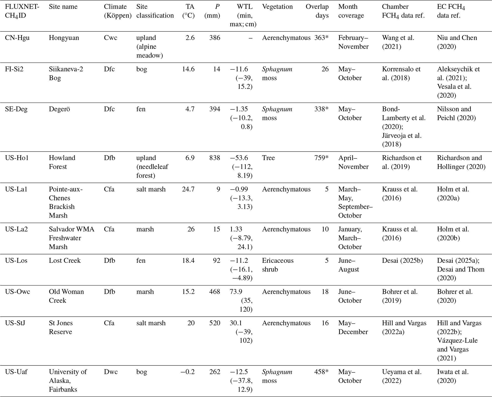
We compiled ecosystem-scale (EC) and plot-scale (chamber) FCH₄ data from ten sites, representing different climatic conditions and ecosystem types (two uplands and eight wetlands; Fig. 1, Table 1). Each site differed in the number of days with both chamber and EC measurements (n=5–759), the number of chambers used (n=3–18), the year of observations (range across sites: 2012–2020), and whether the chambers were automated or manual (Table C1 and Fig. B1). The site selection was based on the availability of coincident EC and chamber FCH₄ data. EC data were obtained from the FLUXNET-CH₄ database (Delwiche et al., 2021; Knox et al., 2019) and chamber data were provided by site principal investigators in response to a call for data via the FLUXNET-CH₄ network. The sites are located in China, Finland, Sweden and the USA. Most sites have a humid continental (n=3) or subarctic climate (n=3), with others located in humid subtropical (n=3) and cold subtropical highland (n=1) regions (Table 1).

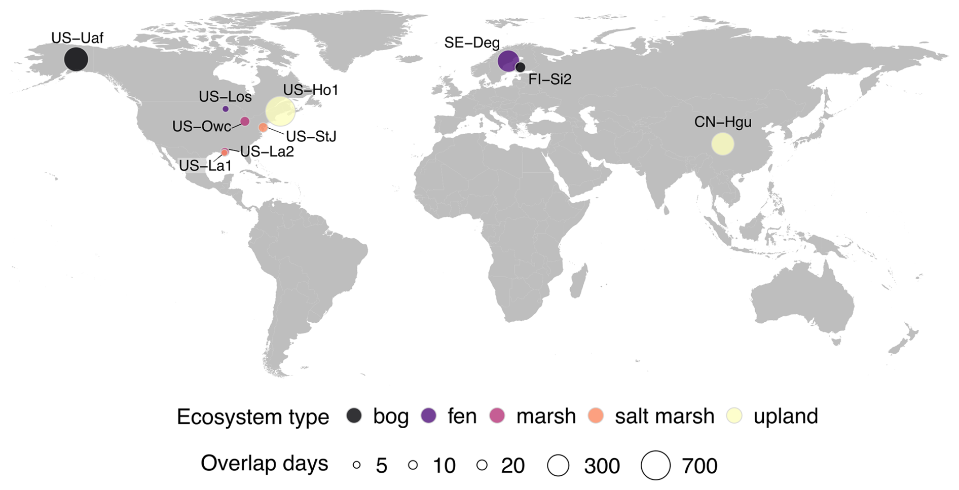
Figure 1 Map of study sites. Point colors indicate ecosystem type and point size reflects the number of overlap days between eddy covariance and chamber measurements (details in Table C1). Ecosystem type follows the site classification in the FLUXNET-CH₄ database (Delwiche et al., 2021; Knox et al., 2019). Base map: Natural Earth (1:50 m Cultural Vectors; https://naturalearthdata.com, last access: 1 September 2025), created with R package maps (Becker et al., 2023). Country abbreviations: CN = China, FI = Finland, SE = Sweden, US = The United States of America.

Table 1 Environmental characteristics of the study sites during the FCH₄ observation periods. Site classification, dominant vegetation, air temperature, precipitation, and water table level data were obtained from half-hourly FLUXNET-CH₄ and chamber datasets (Delwiche et al., 2021; Knox et al., 2019). Mean air temperature, total precipitation, and mean water table level were calculated over the EC-chamber overlap periods used in the analyses. Negative water table level indicates that water table level was below the soil surface. Köppen climate abbreviations: Cwc = cold subtropical highland, Dfc = subarctic, Dfb = warm-summer humid continental, Cfa = humid subtropical, Dwc = monsoon-influenced subarctic climate. Column abbreviations: TA = air temperature, P = total precipitation, WTL = water table level, Vegetation = site dominant vegetation type, Overlap days = number of days with both EC and chamber FCH₄ observations. In Overlap days, values marked with and without asterisk (*) represent automated and manual chambers, respectively. Country abbreviations: CN = China, FI = Finland, SE = Sweden, US = The United States of America.

2.2 Datasets and data compilation

2.2.1 Chamber and EC CH₄ flux data

The FCH₄ data were selected based on coincident plot- and ecosystem-scale FCH₄ observations. The plot-scale chamber FCH₄ data for each site were obtained from the site principal investigators. Each dataset included FCH₄ (varying units) and additional environmental variables, such as soil temperature and water table level. Chamber datasets comprised measurements from both manual (n=6 sites; taken 1–3 times per month) and automated chamber methods (n=4 sites; taken at half-hourly or hourly intervals, see Table C1; Subke et al., 2021). Chamber fluxes for all sites were calculated by the data providers using linear regression of change in CH₄ concentration over time. None of the chamber FCH₄ data were gap-filled, and in some cases (n=4 sites), ebullition events had been filtered out by the data providers (Table C2). The decision to utilize chamber FCH₄ data with differing ebullition removal protocols across data providers was intended to reflect the way ebullition data are dropped in chamber studies. Typically, FCH₄ measurements are excluded from analyses when linear regressions between timepoints fall below a user-defined R² threshold (Jentzsch et al., 2025). These data exclusions may contribute to differences between bulk ecosystem- and plot-scale FCH₄ estimates. We designated CH₄ emission with positive, and CH₄ uptake with negative signs.

The ecosystem-scale EC datasets for each site (except US-StJ, see below) were obtained from the FLUXNET-CH₄ database (Delwiche et al., 2021; Knox et al., 2019). These data include both gap-filled and non-gap-filled FCH₄ values (nmol m⁻² s⁻¹) at a half-hourly resolution along with various meteorological and environmental variables. We used gap-filled EC FCH₄ in the analyses but excluded data during long data gaps (>2 months) when the gap-filled values may be a significant source of uncertainty (Delwiche et al., 2021). Gap-filling was performed using artificial neural networks (ANN; Knox et al., 2019) which have shown good performance for FCH₄ data gap-filling (Irvin et al., 2021; Knox et al., 2016, 2019).

CN-Hgu EC FCH₄ data showed anomalous extreme CH₄ uptake and isolated extreme positive FCH₄ spikes. Therefore, we filtered out EC FCH₄ values where (1) CH₄ uptake exceeded −100 nmol m⁻² s⁻¹ (empirically determined threshold; Chen et al., 2019, 2020), (2) nighttime (incoming shortwave radiation <10 W m⁻²; Morin et al., 2014) friction velocity (u^*) < 0.1 m s⁻¹ (Chen et al., 2019, 2020), and (3) single extreme positive FCH₄ spikes occurred beyond the monthly 99.5th FCH₄ percentile where nighttime air temperature was within 1 °C of its dew point (calculated with Magnus formula and Alduchov & Eskridge constants; Alduchov and Eskridge, 1996; Lawrence, 2005) and the open-path gas analyzer may have had condensation (Heusinkveld et al., 2008). Additional extreme FCH₄ (FCH₄=862 nmol m⁻² s⁻¹) associated with friction velocity = 0.93 m s⁻¹ and wind speed = 0.05 m s⁻¹ was removed as an outlier. After filtering, the CN-Hgu dataset was 70 % of the original.

For US-StJ, we obtained EC FCH₄ data from the data providers (Hill and Vargas, 2022b; Vázquez-Lule and Vargas, 2021). As ANN-gap-filled EC FCH₄ values were not available at US-StJ, we used only non-gap-filled EC FCH₄. EC FCH₄ were processed by the data providers following AmeriFlux protocols (Chu et al., 2023; Hill and Vargas, 2022b; Vázquez-Lule and Vargas, 2021).

2.2.2 Environmental data

For all sites (except US-StJ), environmental data were obtained from the FLUXNET-CH₄ EC data product, including ANN-gap-filled net ecosystem CO₂ exchange (NEE), friction velocity (u^*), wind direction (WD), gap-filled wind speed, gap-filled vapor pressure deficit (VPD), and gap-filled air pressure (PA) (Delwiche et al., 2021; Knox et al., 2019). Soil temperature (TS; topmost 2–10 cm depth) data was obtained from FLUXNET-CH₄ and site-specific chamber datasets when available. If a site had TS observations from both chamber and FLUXNET-CH₄ datasets, a mean of both was taken to obtain a site-level TS. Similarly, site-level water table level (WTL) was obtained by utilizing either FLUXNET-CH₄ or chamber-associated WTL measurements, or by taking their mean.

Environmental data for US-StJ were obtained from the data providers (Hill and Vargas, 2022b; Vázquez-Lule and Vargas, 2021). PA, VPD, wind speed, WD, and u^* were not gap-filled, while TS and WTL were gap-filled based on their linear relationships with water temperature and water table level, respectively (Hill and Vargas, 2022b). NEE was gap-filled using marginal distribution sampling moving look-up tables (Hill and Vargas, 2022b).

See a summary of environmental data in Table C3.

2.3 Data processing and harmonization

The chamber datasets were harmonized to a similar structure, and FCH₄ units were standardized to nmol m⁻² s⁻¹, matching the units used in the FLUXNET-CH₄ EC FCH₄ data. Then, EC and chamber datasets were combined using common timestamps (Fig. 2). To evaluate differences across temporal aggregations, we aggregated data at six temporal scales: (1) half-hourly (automated chamber data only; CN-Hgu, SE-Deg, US-Ho1, US-Uaf; n=4 sites), (2) hourly (CN-Hgu, SE-Deg, US-Ho1, US-Uaf; n=4 sites), (3) daily (all sites, n=10 sites), (4) weekly (n=10 sites), (5) monthly (n=10 sites), and (6) annual (n=10 sites) (Fig. 2). Note that most sites did not include snow-covered periods, and the datasets primarily represent the snow-free season.

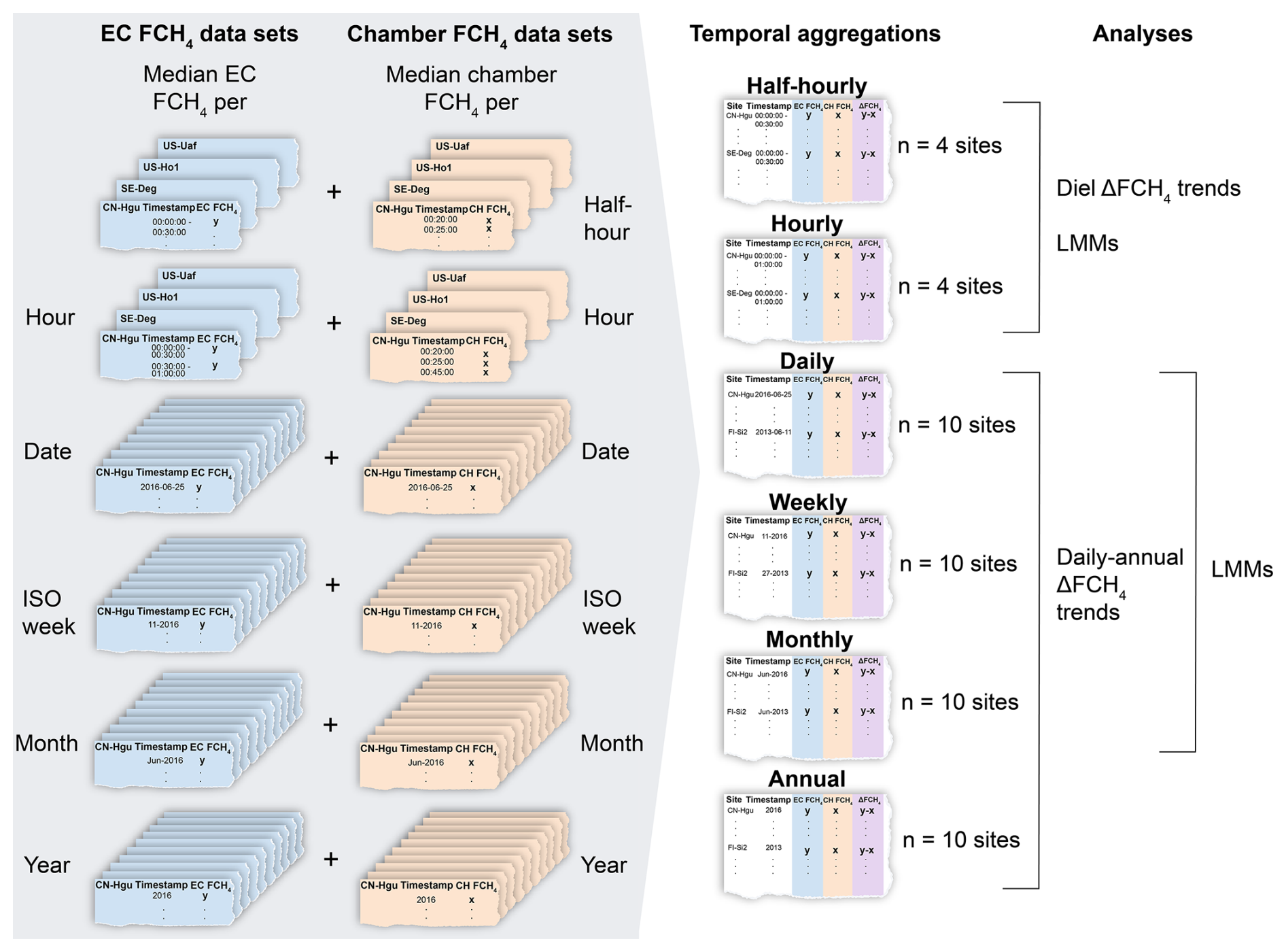
Figure 2 Overview of the main data aggregation workflow. Site-specific eddy covariance (EC) methane (CH₄) flux (FCH₄; blue) and chamber FCH₄ (orange) datasets were combined by taking the median FCH₄ per timestamp (half-hour to annual scale). ISO week is the week number according to the ISO-8601 standard. Then, site-level datasets were combined into multi-site datasets at six temporal scales: half-hourly, hourly, daily, weekly, monthly, and annual. Half-hourly EC FCH₄ data was not aggregated as it was already in half-hourly scale. ΔFCH₄ (purple) was calculated by subtracting median chamber instantaneous FCH₄ from median EC instantaneous FCH₄ per timestamp per site, and this measure was used in all analyses and linear mixed effects models (LMMs). Note that we also created temporal aggregations by taking the mean of EC and chamber FCH₄, and these data sets were used as a sensitivity check with descriptive statistics and pairwise comparisons.

The data were aggregated from the timestamp-aligned data by taking the median of FCH₄ measurements (non-normally distributed), mean of NEE (normally distributed) and wind u and v components (see Sect. 2.4.2), and median of the rest of the environment and meteorological variables (non-normally distributed). Half-hourly aggregation was created by taking the median of chamber measurements for each EC timestamp. To check for robustness of our results from the median-based temporal aggregations, we also created temporal aggregations based on FCH₄ means. In addition, we calculated cumulative sums (mg CH₄ m⁻²) of chamber and EC FCH₄ at daily, weekly, monthly, and annual scales to see how EC-chamber differences scale up to ecosystem CH₄ budgets. As the chamber FCH₄ data from FI-Si2, US-La1, and US-La2 lacked hourly timestamps, we estimated daily cumulative FCH₄ for these sites by using the daily median or mean chamber FCH₄ and multiplied it by 48 while EC cumulative FCH₄ was calculated based on half-hourly EC FCH₄ from FLUXNET-CH₄. As this is not an accurate estimate of daily cumulative chamber FCH₄ for EC-chamber FCH₄ comparisons, we included these sites only in site-specific analyses and excluded them from cross-site analyses.

The difference between ecosystem and plot-scale FCH₄ was calculated as the row-wise difference between instantaneous EC FCH₄ and chamber FCH₄ (ΔFCH₄) in each aggregated dataset by subtracting chamber FCH₄ from the corresponding EC FCH₄ on the same timestamp. For supplementary analyses, we calculated the difference between cumulative EC FCH₄ and chamber FCH₄ at daily, weekly, monthly, and annual scales.

2.4 Statistical analyses

2.4.1 Differences between ecosystem and plot-scale FCH₄ observations

We used non-parametric statistics to analyze the FCH₄ data (EC, chamber and ΔFCH₄), because the data were skewed and non-normal. To test the statistical significance (α = 0.05) of ΔFCH₄ and to assess ΔFCH₄ differences between chamber types at different temporal scales, we used Wilcoxon-Mann-Whitney tests (wilcox.test from stats; R Core Team, 2024). Since the mean-based temporal aggregations were used as a sensitivity check, only descriptive statistics and Wilcoxon-Mann-Whitney tests were conducted for the mean-based aggregations (results in Table C4). Similarly, cumulative FCH₄ were analyzed with descriptive statistics and Wilcoxon-Mann-Whitney tests (results in Table C5). The rest of the methods described here were conducted on the median-based temporal aggregations of instantaneous FCH₄.

To estimate the slopes of the EC FCH₄–chamber FCH₄ relationship, we built simple linear mixed effects models with site as the random effect using function lme from package nlme (Pinheiro and Bates, 2000; Pinheiro et al., 2023). For better interpretability of model slopes (in contrast to Yeo-Johnson-transformed values, see Sect. 2.4.2) and to meet the residual normality assumptions of linear mixed modeling, we transformed EC FCH₄ with inverse hyperbolic sine (Table C6). Due to non-convergence and residual non-normality, half-hourly and hourly scales were not assessed for EC-chamber FCH₄ slopes. As the data were non-normally distributed and did not meet the assumptions of linear regression, we used Spearman correlations together with normalized root mean square error (using the standard deviation of pooled EC and chamber FCH₄ as the denominator at each temporal scale) to assess the direction and strength of the relationship between EC FCH₄ and chamber FCH₄, manual and automated chamber FCH₄, as well as FCH₄ magnitude (row-wise mean of EC and chamber FCH₄) and absolute ΔFCH₄.

We used Kruskal-Wallis tests (kruskal.test from stats; R Core Team, 2024) to test for differences in ΔFCH₄ across hours and months (treated as categorical variables) within each temporal aggregation (half-hourly, hourly, daily, weekly, monthly, and annual). Then, we identified the significantly differing groups using the Conover-Iman post hoc test (function conover.test from package conover.test; Dinno, 2024).

2.4.2 Predictors of FCH₄ differences between ecosystem and plot scales

We built linear mixed models to estimate the predictors of ΔFCH₄. The aim was to explore how the predictors influence the direction of ΔFCH₄ (i.e., more positive or negative ΔFCH₄ or, in other words, increase ecosystem-scale FCH₄ in relation to plot-scale FCH₄ or vice versa) at the ten sites. To meet the assumptions of linear mixed modeling and to improve residual diagnostics (normality and homoscedasticity of residuals) for model inference, we applied Yeo-Johnson power transformation (Yeo and Johnson, 2000) to absolute ΔFCH₄ values using the function yeojohnson from bestNormalize (Peterson, 2021). This transformation can be applied to zero values, and it improved our residual diagnostics, which were important for model inference. Acknowledging the difficulty to interpret the precise effect sizes after this transformation, we used this model only to investigate the directionality of ΔFCH₄. All models were built with the function lme from nlme (Pinheiro and Bates, 2000; Pinheiro et al., 2023).

To evaluate potential predictors of ΔFCH₄, we included environmental and temporal variables available in the FLUXNET-CH₄ and chamber datasets in the models. The predictor selection was based on literature. They included: TS (°C), WTL (cm), PA (kPa), u^* (m s⁻¹), WD (degrees), VPD (hPa), NEE (µmol CO₂ m⁻² s⁻¹), month (categorical), site dominant vegetation (VEG; categorical; “tree”, “ericaceous shrub”, “aerenchymatous”, “brown moss”, and “Sphagnum moss”; taken from Delwiche et al., 2021), and hour (categorical; only with half-hourly and hourly datasets). We included EC-specific variables, such as u^* and WD, as proxies for EC footprint to assess how variables contributing to the EC footprint may affect ΔFCH₄. While two of the VEG classes (tree and ericaceous shrub) were only represented in one site, preliminary linear regression model comparisons showed that VEG explained a large proportion of the ΔFCH₄ variance (R²=0.4–0.7), and its inclusion in linear mixed models substantially improved model fit. Therefore, we included VEG as a fixed effect, while acknowledging that for tree and ericaceous shrub classes, the estimated effect may be related to the site rather than vegetation.

For all models, the reference level in VEG was Sphagnum moss, 0 in Hour, and May in Month. As WD is a circular variable (0° = 360°), we represented WD as a continuous function of wind direction and speed by separating WD into orthogonal u and v wind components (uWD and vWD, respectively), which were averaged from the half-hourly EC datasets in hourly, daily, weekly, monthly, and annual aggregations (Appendix A1). As a result, uWD represents the strength of west-east wind while vWD represents the strength of north-south wind. This representation avoided discontinuity at 360° = 0° and potential multicollinearity between model predictors.

For improved model convergence and β-coefficient calculations, Yeo-Johnson-transformed absolute ΔFCH₄ and all predictors were centered and scaled, except hour, month and VEG, which were categorical variables and were included without centering and scaling. To account for multicollinearity, we chose predictors based on Pearson correlation matrices (threshold $\left|r\right|\mathit{<}\mathrm{0.7}$) and checked variance inflation factors (VIF; threshold ≤ 3) using the function vif from car (Fox and Weisberg, 2018). Due to multicollinearity (VIF > 3), we built two separate half-hourly models containing either month or TS, two weekly models without NEE or VPD, and a monthly model without VPD and TS. WTL data was not available for CN-Hgu, and thus, this site was excluded from the models.

After accounting for temporal autocorrelation and residual variance (Appendix A2), we used backward variable selection based on likelihood ratio tests (AIC and p-values) together with type I ANOVA tests to determine significant predictors of Yeo-Johnson-transformed absolute ΔFCH₄. During variable selection, the models were fitted with maximum likelihood, and the final models were refitted with restricted maximum likelihood for statistical inference. Model marginal and conditional R² were calculated with the function r.squaredGLMM from package MuMIn (Bartoń, 2024). To test how well the models generalize to other sites, we validated the models with leave-one-site-out cross validation and evaluated model performance with R², mean absolute error (MAE) and root mean square error (RMSE) between observed and predicted values. To allow for predictions to new sites with the training data, the fixed effect VEG had to be removed from the models, as some of the VEG classes (tree and ericaceous shrub) were represented only by a single site and the effect of these classes cannot be estimated when they are withheld in the test data. Similarly, due to uneven temporal coverage across sites, observations (e.g., date or year-month) included in the test data but not present in the training data were excluded from evaluation.

We built linear mixed effects models to investigate the effect of spatiotemporal FCH₄ variation on ΔFCH₄. To represent the FCH₄ variation between individual chambers within each site, we calculated the interquartile range (IQR) of chamber FCH₄ from an unaggregated dataset per each site and temporal scale unit (i.e., per day, week, month, or year). To see whether temporal variation within each temporal scale unit in EC FCH₄ may affect absolute ΔFCH₄, we also calculated EC FCH₄ IQR per each site and temporal scale unit. In the models, log-transformed absolute ΔFCH₄ was the response variable, and either log (+0.01)-transformed chamber IQR or log (+0.01)-transformed EC IQR was the explanatory variable, or both were included as explanatory variables to assess their relative effects on absolute ΔFCH₄.

All data processing and statistical analyses were carried out using R v4.3.3 (R Core Team, 2024).

3 Results

3.1 Ecosystem and plot-scale FCH₄ differ most at finer temporal scales

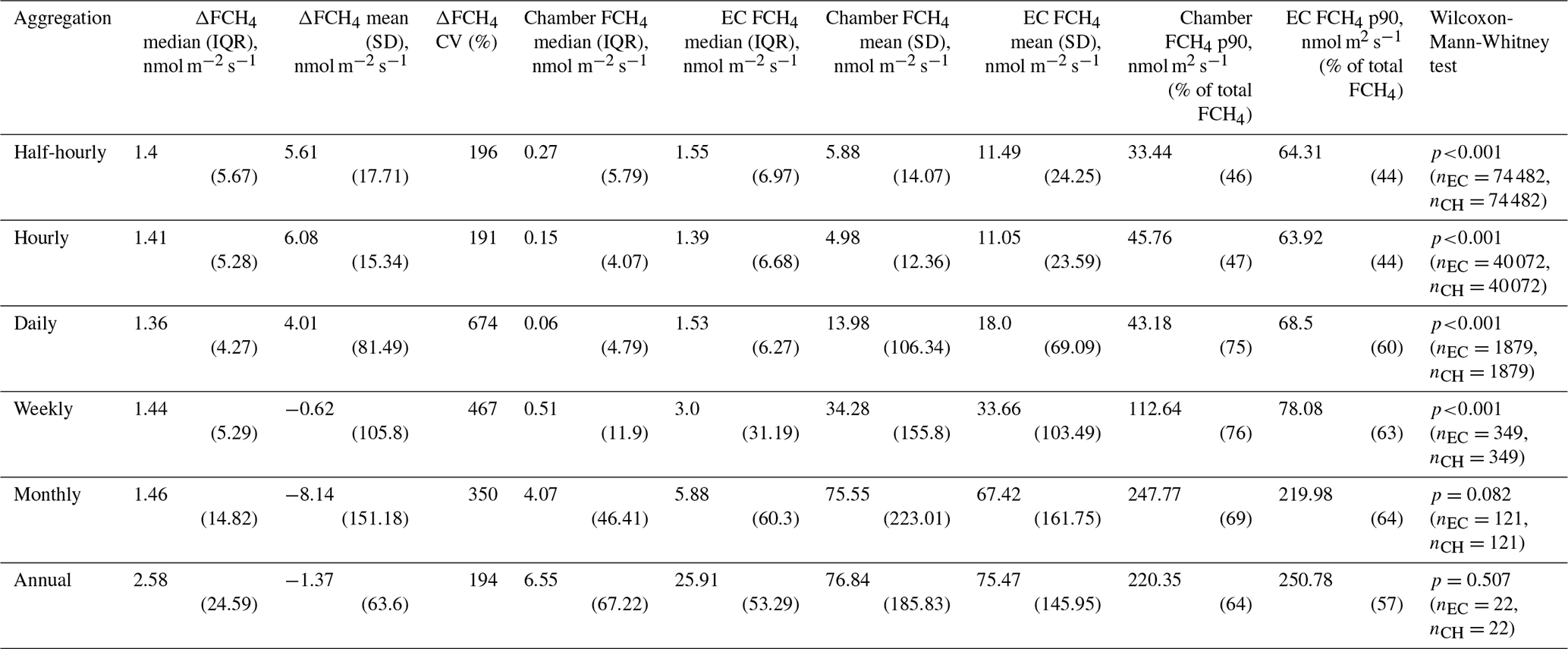
Ecosystem- (EC) and plot-scale (chamber) FCH₄ differed significantly at half-hourly to weekly scales (Table 2). Median ecosystem FCH₄ was higher than plot-scale FCH₄ at all temporal aggregations (half-hourly to annual: 102 %, 109 %, 104 %, 90 %, 58 %, and 87 % higher, respectively). However, the coefficient of variation (CV, %) for ΔFCH₄ was large, particularly in daily (674 %) and weekly (467 %) aggregations (Table 2). Across temporal aggregations and site-years, CH₄ emissions (FCH₄ > 0) above the 90th percentile contributed a larger share of total (sum) plot-scale FCH₄ than ecosystem-scale FCH₄ (mean-based aggregations; Table 2, Fig. B2), possibly indicating more CH₄ emission hot spots and hot moments at the plot scale. Our observed trend persisted when we aggregated chamber and EC FCH₄ data with means instead of medians (Tables C4 and C5). In the mean-based aggregations, median ΔFCH₄ ranged between 0.28 nmol m⁻² s⁻¹ (annual) and 1.23 nmol m⁻² s⁻¹ (half-hourly) but mean ΔFCH₄ turned increasingly negative from daily (−1.16 nmol m⁻² s⁻¹) to annual (−70.94 nmol m⁻² s⁻¹) scales, highlighting plot-scale CH₄ emission hotspots and hot moments as possible ΔFCH₄ drivers. Ecosystem- and plot-scale FCH₄ were positively correlated across temporal aggregations, with annual aggregation having the best agreement, while the worst agreements were in half-hourly and hourly aggregations (Fig. 3). Using linear mixed models, we showed that an increase of 1 nmol m⁻² s⁻¹ in plot-scale FCH₄ was associated with an ecosystem-scale FCH₄ increase of 0.007 nmol m⁻² s⁻¹ (p=0.03) at daily plot-scale FCH₄ median (0.06 nmol m⁻² s⁻¹), 0.01 nmol m⁻² s⁻¹ (p=0.066) at weekly plot-scale FCH₄ median (0.51 nmol m⁻² s⁻¹), 0.009 nmol m⁻² s⁻¹ (p=0.183) at monthly plot-scale FCH₄ median (4.07 nmol m⁻² s⁻¹), and 0.019 (p=0.044) at annual plot-scale FCH₄ median (6.55 nmol m⁻² s⁻¹; see Table C6 for details).

Table 2 Ecosystem- (eddy covariance; EC) and plot-scale (chamber) methane (CH₄) flux (FCH₄) difference (ΔFCH₄) at different temporal aggregations. A positive ΔFCH₄ indicates a higher ecosystem- than plot-scale FCH₄ and vice versa. The EC and chamber data sample sizes in Wilcoxon-Mann-Whitney tests are reported as n_EC and n_CH, respectively. The 90th percentiles (p90, without parentheses) and proportion (%, in parentheses) of chamber and EC CH₄ emission observations (where FCH₄ > p90 and FCH₄ > 0) of the total chamber or EC FCH₄ sum show the contribution of high CH₄ emissions to total CH₄ emissions (see site-specific trends in the unaggregated dataset in Fig. B2). Abbreviations: IQR = interquartile range, SD = standard deviation, CV =  coefficient of variation.

Ecosystem- and plot-scale FCH₄ differed between hours, months, and sites. In support of our hypotheses, the highest ΔFCH₄ occurred between 5 AM and 3 PM (p<0.001; Figs. B4–B7), with maximum median ΔFCH₄ at 9 AM (2.01 nmol m⁻² s⁻¹, IQR: 6.16; half-hourly scale) and minimum at 8 PM (0.9 nmol m⁻² s⁻¹, IQR: 4.16; half-hourly scale). However, the diel ΔFCH₄ trends varied between sites and months (p<0.001; Figs. B8–B12). The highest absolute ΔFCH₄ (with observations from all sites) was in August, September, and October (half-hourly to daily p<0.001; Fig. B13). In addition, ΔFCH₄ varied in both magnitude and direction within and between sites (Kruskal-Wallis p<0.001; half-hourly to monthly scale), with most medians being positive (Tables C6–C11 and Figs. B14–B15). The difference between cumulative sums of ecosystem- and plot-scale FCH₄ increased from daily to annual scales but the seasonal and inter-annual trends varied between sites (Table B4, Fig. B16). The largest absolute ΔFCH₄ medians and CVs were consistently found in US-Owc (median: −108.22 nmol m⁻² s⁻¹, CV: 169 %; daily scale), while the lowest absolute ΔFCH₄ and FCH₄ were consistently found in US-Ho1 (median ΔFCH₄ < 1 nmol m⁻² s⁻¹; Tables C6–C11).

Flux magnitude, measured as the mean between EC and chamber FCH₄ (FCH_{4_mean}), was generally positively related to ΔFCH₄ but negative relationships existed when FCH_{4_mean} < 0 (i.e., net uptake). The positive FCH₄ magnitude and absolute ΔFCH₄ relationship became stronger at coarser temporal resolutions (Spearman p<0.001; Fig. 4). In all aggregations, the higher ΔFCH₄ came from a higher ecosystem-scale FCH₄ than from a higher plot-scale FCH₄ (≥70 % of all observations when FCH_{4_mean} > 0; result not shown). In half-hourly and hourly aggregations, ΔFCH₄ and FCH_{4_mean} were negatively or positively related when FCH_{4_mean} suggested net uptake or emission, respectively (Fig. 4a and b). When FCH_{4_mean} < 0, ecosystem-scale FCH₄ was generally higher than plot-scale FCH₄ (57 % and 58 % of all observations when FCH_{4_mean} < 0 in half-hourly and hourly aggregations, respectively; result not shown). However, most of the highest observations originate from CN-Hgu. Sites also differed in whether the trends in negative FCH₄ came from higher plot or ecosystem-scale FCH₄: for example, at US-Uaf and CN-Hgu, 100 % and 91 % of ΔFCH₄ observations at FCH_{4_mean} < 0, respectively, consisted of higher plot-scale FCH₄ while ca. 66 % of hourly and half-hourly observations (FCH_{4_mean} < 0) in US-Ho1 came from higher ecosystem-scale FCH₄.

3.2 Predictors of ecosystem and plot-scale FCH₄ differences

3.2.1 Atmospheric pressure, friction velocity and wind direction drive daily-to-monthly FCH₄ differences between ecosystem and plot scales

The significance and effect size of ΔFCH₄ predictors varied across temporal aggregations, with site dominant vegetation type having the highest effect sizes at the daily-to-monthly scale (Table 3). Dominance of aerenchymatous vegetation had relatively high effect sizes ($\left|\mathit{\beta }\text{-coefficient}\right|$ > 0.68). However, only one site was classified as tree-dominated (US-Ho1) and ericaceous shrub-dominated (US-Los), while three were aerenchymatous and two were Sphagnum-moss dominated. Thus, we were unable to separate true vegetation-related effects from site effects.

Table 3 Linear mixed effects model results identifying environmental predictors of ecosystem- and plot-scale methane (CH₄) flux (FCH₄) difference (ΔFCH₄) at different temporal scales. Fixed effects are listed in decreasing order based on their β-coefficients. Significant predictors are highlighted in bold. Half-hourly and hourly models had very low marginal R² (<0.05) and were excluded from this table. See half-hourly and hourly models in Table C14 and full models in Table C15. Abbreviations: SE = standard error, Df = degrees of freedom, LOOCV = leave-one-out cross validation, MAE = mean absolute error, RMSE = root mean square error, VEG = site dominant vegetation, PA = air pressure (kPa), u^* = friction velocity (m s⁻¹), WTL = water table level (cm), TS = soil temperature (°C), NEE = net ecosystem CO₂ exchange (µmol CO₂ m⁻² s⁻¹), VPD = vapor pressure deficit (hPa), vWD = v wind component (m s⁻¹), uWD = u wind component (m s⁻¹).

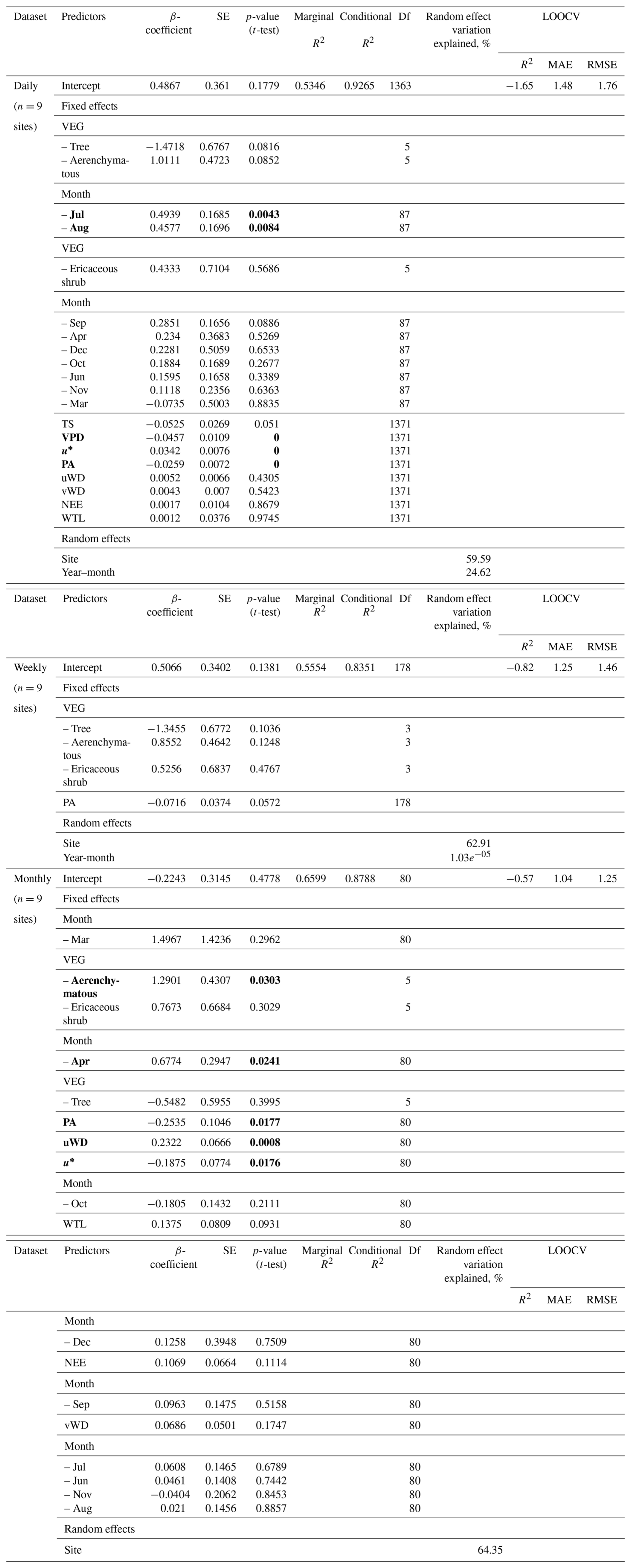
PA and u^* were significant ΔFCH₄ predictors at the daily and monthly scales (but weekly PA p=0.057), while VPD was significant only at the daily scale. However, the effect sizes were relatively low (β-coefficient ≤ 0.25; Table 3). Wind direction (uWD) was a significant ΔFCH₄ predictor only in the monthly scale. Month was a significant predictor only in the final half-hourly-daily models, where August and July had the highest effect sizes (β-coefficient > 0.41). Morning hours, particularly 5 AM, were most important in the half-hourly-hourly models (5 AM β-coefficient > 0.08). However, the fixed effects in the final half-hourly and hourly models explained a very small proportion of the total variation (marginal R²<0.05, Tables C14–C15). In addition, the high conditional R² and high negative LOOCV R², high MAE and RMSE showed that the ΔFCH₄ predictors are specific to the sites included in this study (Table 3).

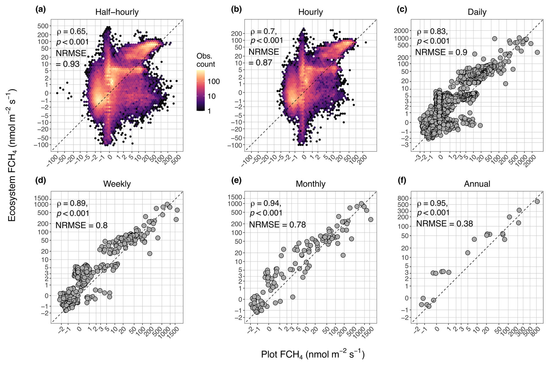
Figure 3 Results of correlation test (Spearman rank correlation coefficient, ρ, its significance level, p, and the normalized root mean square error, NRMSE) between plot-scale (chamber) methane (CH₄) flux (FCH₄) and ecosystem-scale (eddy covariance; EC) FCH₄ at half hourly (a), hourly (b), daily (c), weekly (d), monthly (e), and annual scales (f). For visualization, the plot axes (a–f) were transformed with inverse hyperbolic sine to spread out points in the low FCH₄ range and retain negative values (see untransformed plots in Fig. B3). Spearman ρ was calculated with untransformed data. NRMSE was calculated by dividing RMSE by the standard deviation of untransformed ecosystem- and plot-scale FCH₄ at each temporal aggregation. In (a) and (b) the points for half-hourly (n=74 482) and hourly (n=40 072) aggregations are shown in hexagonal density clouds with log10-transformed color range to highlight trends in high point density areas (colors represent number of observations per hexagon). Agreement between chamber and EC FCH₄ improves from finer to coarser temporal aggregations (a–f), as indicated by ρ. The high observation densities in(a) and (b) reveal site-specific trends in the discrepancy between ecosystem and plot scales (e.g., at x=0 and y=5). For daily (c), weekly (d), monthly (e), and annual (f) aggregations, sample sizes were n=1879, 349, 121, and 22, respectively. The dashed line represents 1:1 line.

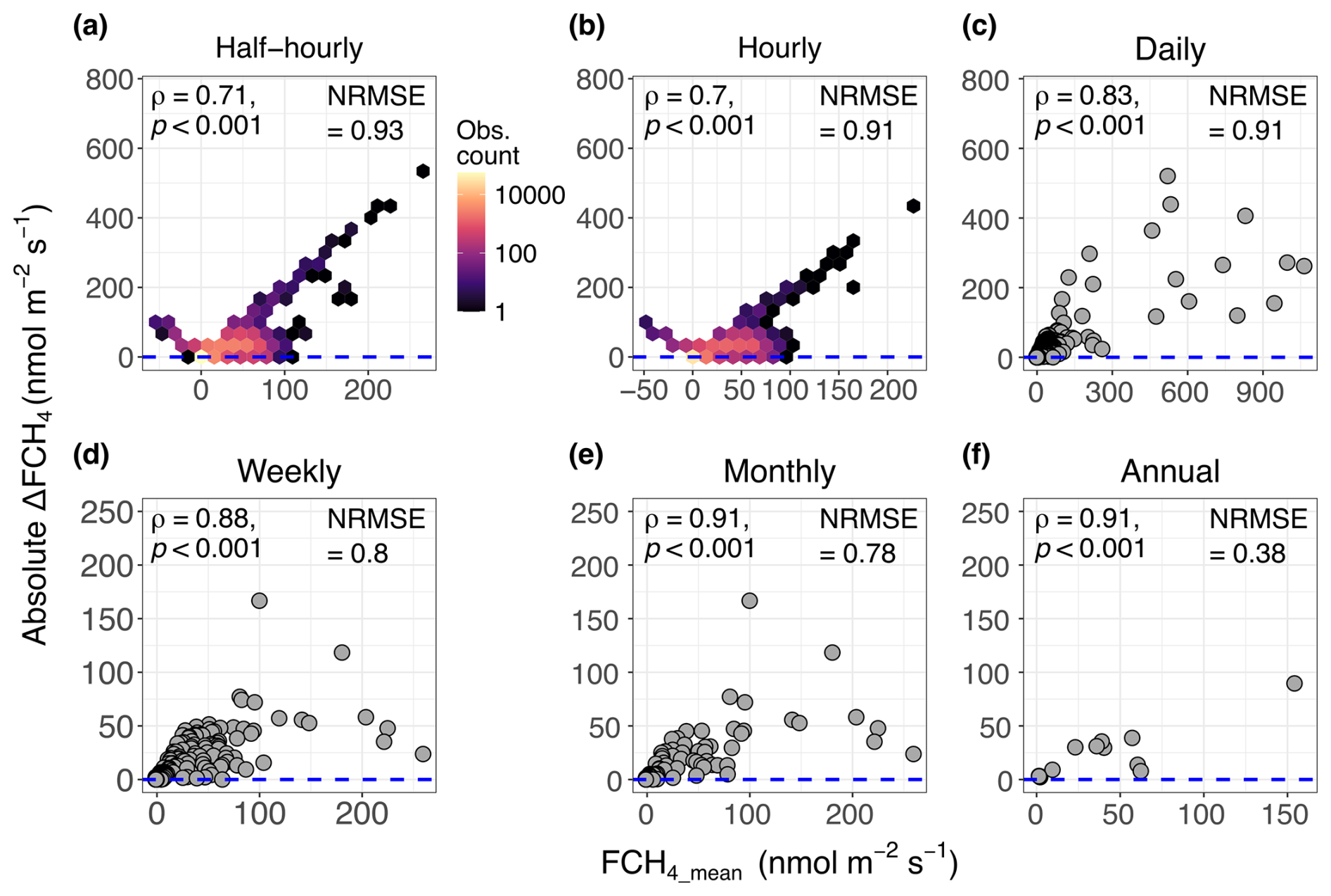
Figure 4 The relationship between methane (CH₄) flux (FCH₄) magnitude (FCH_{4_mean}) and absolute difference between ecosystem-scale (eddy covariance; EC) and plot-scale FCH₄ (ΔFCH₄) from half-hourly (a) to annual (f) scales, represented by Spearman correlation coefficient, (ρ), its significance, (p), and normalized root mean square error of ΔFCH₄ (NRMSE). FCH_{4_mean} is the row-wise mean of EC FCH₄ and chamber FCH₄. In(a) and (b) half-hourly and hourly points are shown in hexagonal density clouds with a log-transformed color range to highlight trends in high point density areas (colors represent number of observations per hexagon). Plots (c)–(f) show daily, weekly, monthly and annual aggregations, respectively. The blue dashed line represents ΔFCH₄=0 meaning complete agreement between ecosystem and plot-scale FCH₄. Higher Spearman correlation coefficient (α = 0.05) represents stronger deviation from ΔFCH₄=0. NRMSE was calculated by dividing RMSE (of ΔFCH₄) by the standard deviation of ecosystem- and plot-scale FCH₄ at each temporal aggregation. For visualization, outliers were removed from daily (n=3), weekly (n=10), monthly (n=8) and annual (n=1) plots but the Spearman correlations and NRMSE are based on original data. See plots with outliers in Fig. B17 and a figure showing how high CH₄ emissions from ecosystem and plot scales contribute to annual CH₄ emissions per site in Fig. B2.

3.2.2 Spatial FCH₄ variation increases ecosystem and plot-scale FCH₄ difference

Spatial variation between FCH₄ measurements by individual chambers increased absolute ΔFCH₄ (Fig. 5). The increasing trend between chamber IQR (log + 0.01) and absolute ΔFCH₄ (log) became clearer in coarser temporal scales, where a unit (e-fold; ca. 2.7×) increase in monthly and annual chamber FCH₄ variation (IQR + 0.01) was associated with ca. 51 % and 63 % increase in absolute ΔFCH₄, respectively (marginal R²≥0.31, p≤0.01). Temporal EC FCH₄ variation (e.g., within date at the daily scale) did not lead to strong increases in absolute ΔFCH₄ at daily-to-monthly aggregations (marginal R² < 0.01), but the annual mixed effects model showed a ca. 198 % increase in absolute ΔFCH₄ with a unit increase in EC FCH₄ IQR (+0.01; marginal R²=0.82). Models with both chamber and EC IQR (log + 0.01) as explanatory variables showed significant chamber IQR at daily-to-monthly aggregations (p<0.001, marginal R²=0.06–0.31) and significant EC IQR at daily scale (p=0.005). In contrast, the annual model had a nonsignificant chamber IQR and significant EC IQR (p=0.001, marginal R²=0.81). The sites also differed in the strength and direction of the relationship between chamber and EC FCH₄ variation and ΔFCH₄ (Fig. 5).

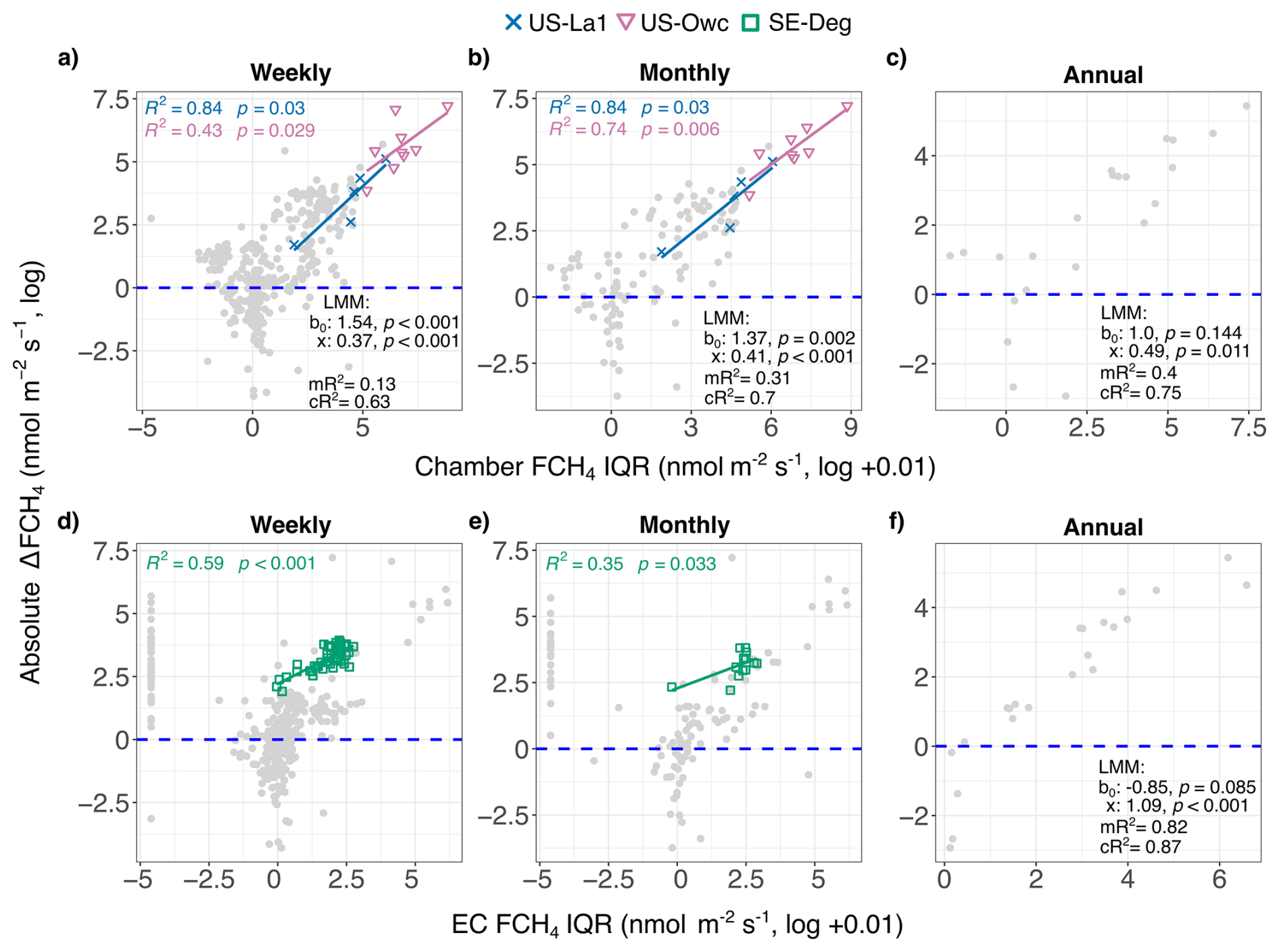
Figure 5 Variation in methane (CH₄) flux (FCH₄) between individual chambers and eddy covariance (EC) timestamps increases absolute ΔFCH₄. (a–c) Relationship between chamber FCH₄ variation (variation between individual chambers per aggregation timestamp, represented by interquartile range; IQR) and absolute ΔFCH₄ at weekly (a), monthly (b) and annual (c) scales. (d–f) Relationship between EC timestamp FCH₄ variation (represented by IQR) and absolute ΔFCH₄ at weekly (d), monthly (e) and annual (f) scales. Linear mixed effects model (LMM) results: b₀ = model intercept, x = predictor (chamber or EC FCH₄ log IQR + 0.01) of log absolute ΔFCH₄, p = predictor significance (preceded by model coefficient estimates), mR² and cR² = marginal and conditional R², respectively. In (d) and (e) LMM results are not shown due to low marginal R² (mR² ≤ 0.06). In (e) linear regression results for SE-Deg without data point where x<0: R²=0.62 p=0.002. Daily scale is not shown due to the low number (n=1) of sites with significant relationships and low marginal R² (mR² ≤ 0.06). Linear regressions, R²s and p-values are only shown for sites with significant IQR predictor and R²>0.2 and are shown in different colors and shapes (gray points: nonsignificant and R²≤0.2 sites). The dashed blue line indicates ΔFCH₄=0. See version with untransformed data in Fig. B18.

3.2.3 Ecosystem and plot-scale FCH₄ difference does not significantly vary among chamber types

We did not find significant differences in ΔFCH₄ between automated and manual chambers at all aggregations (Wilcoxon-Mann-Whitney; daily p=0.948, weekly p=0.361, monthly p=0.565, annual p=0.722). However, ΔFCH₄ in manual chambers had higher variation than automated chambers at the daily (CV_manual=284 %, CV_automated=181 %), weekly (CV_manual= 262 %, CV_automated=181 %), and monthly (CV_manual=240 %, CV_automated=182 %) scales. The correlations between chamber FCH₄ and EC FCH₄ for both automated and manual chambers were strong at the daily-to-annual scales (ρ>0.7, Fig. B19).

4 Discussion

4.1 Ecosystem-scale FCH₄ is higher than plot-scale FCH₄ at all temporal scales

As a first step to reconcile the discrepancies in FCH₄ data obtained from ecosystem-scale EC and plot-scale chamber measurements, we explored the cross-scale differences across ten sites and six temporal aggregations. Across all temporal scales, ecosystem-scale (EC) FCH₄ was higher than at the plot scale (chamber). Supporting these results, higher EC FCH₄ than chamber FCH₄ have been observed in an arctic peatland with area-weighted chamber FCH₄ (Budishchev et al., 2014), a managed peat meadow with upscaled chamber FCH₄ (Schrier-Uijl et al., 2010), a peatland with down-scaled EC FCH₄ (Forbrich et al., 2011), a temperate forest with spatial chamber FCH₄ averages (Wang et al., 2013), and a temperate salt marsh with spatio-temporal chamber and EC FCH₄ averages (Hill and Vargas, 2022b). Other studies at individual sites have observed higher chamber FCH₄ (upscaled to ecosystem-level with different methods) than EC FCH₄ (Chaichana et al., 2018; Clement et al., 1995; Davidson et al., 2017; Krauss et al., 2016; Marushchak et al., 2016; Meijide et al., 2011; Morin et al., 2017; Riutta et al., 2007). Nonetheless, the median difference was relatively low across sites and temporal aggregations (min 1.36 daily, max 2.58 nmol m⁻² s⁻¹ annual), with CV ranging from a minimum of 191 % (hourly) to a maximum of 674 % (daily; Table 2), indicating relatively good agreement between ecosystem and plot-scale FCH₄ across sites despite high variability. While our higher ecosystem- than plot-scale FCH₄ trend was robust across temporal scales, due to the limited data availability (n=10 sites), our results reflect site differences and generalizations should be tested when more data become available.

We found the best general agreement between instantaneous ecosystem- and plot-scale FCH₄ at the monthly and annual aggregations, with the agreement improving from fine to coarse temporal resolutions. The improved agreement is likely a result of the data aggregation, which reduces the influence of inter-daily FCH₄ variability and inflates correlation coefficients (e.g., Clark and Avery, 1976; Pollet et al., 2015). In addition, mean ΔFCH₄ at the weekly, monthly, and annual scales was negative (i.e., higher plot-scale than ecosystem-scale FCH₄; Table 2), and the CV for the weekly aggregation in particular was large (467 %) (Table 2). These results indicate that high CH₄ emissions and FCH₄ variability in plot-scale measurements are associated with more negative ΔFCH₄, particularly at time scales longer than daily (Table 2 and Fig. B2). This suggests that combining plot- and ecosystem-scale bulk FCH₄ at heterogeneous sites is particularly problematic at coarse temporal scales. However, footprint-aware comparisons between upscaled chamber or downscaled EC FCH₄ could show better agreement between ecosystem and plot scales (e.g., Schrier-Uijl et al., 2010) (see Sect. 4.6). Nonetheless, these results highlight the practice of selective chamber placement on high-emitting locations and time periods (Hill and Vargas 2022b; Vargas and Le, 2023). However, our results based on cumulative FCH₄ (Table C5) also show that ecosystem-scale cumulative FCH₄ are generally higher than at plot scale. Therefore, site-level CH₄ budgets calculated with ecosystem-scale FCH₄ data can exceed plot-scale estimates despite localized plot-scale CH₄ emission peaks (with site-specific variation; Fig. B16).

Mismatches in capturing site FCH₄ heterogeneity, and chamber measurement artifacts may have contributed to the higher ecosystem-scale FCH₄ and ΔFCH₄ variation. Chamber measurements are challenged by tall vegetation and ebullition events are often discarded, which could artificially bias chamber FCH₄ estimates. The EC footprints may have covered high-CH₄-emitting areas (i.e., CH₄ emission hot spots) and ebullition events (i.e., CH₄ emission hot moments) more often than chambers, increasing ΔFCH₄. Although ebullition can also be triggered by chamber placement onto waterlogged soil surface (e.g., Jentzsch et al., 2025), ebullition events were removed from some of the chamber FCH₄ data (see Sect. 2.2.1 and Table C2), so this was unlikely to contribute to the general ΔFCH₄ trends. Indeed, in spatially heterogeneous areas, CH₄ emission hot spots within EC footprints can be important ΔFCH₄ drivers (Desai et al., 2015; Rey-Sanchez et al., 2025; Xu et al., 2018), and at some sites, the majority of FCH₄ is contributed through ebullition (Männistö et al., 2019; Ueyama et al., 2023b; Villa et al., 2021). FCH₄ hot spots and hot moments can also vary in space and time, which manual chamber FCH₄ measurements (n=6 sites) may not capture due to sporadic daytime measurements in weekly or monthly intervals (Anthony and Silver, 2021, 2023; Vargas and Le, 2023). This may result in uncertainties in spatio-temporal FCH₄ and ΔFCH₄ variation across temporal scales (Anthony and Silver, 2021, 2023; Vargas and Le, 2023). The EC footprint effects could be further highlighted by the increasing ΔFCH₄ with greater FCH₄ (Fig. 4), and similar trends were observed in a rice paddy where plot-scale FCH₄ was higher than at ecosystem scale (Meijide et al., 2011). In addition, high CH₄ uptake at the plot scale increased ΔFCH₄ particularly at CN-Hgu (see Sect. 3.1), highlighting selective chamber placement on CH₄-consuming areas (Table C2). However, ΔFCH₄ in low FCH₄ is uncertain due to EC and chamber detection limits, the reported ranges of which cover the minimum absolute ΔFCH₄ of 0–0.05 nmol m⁻² s⁻¹ (Desai et al., 2015; Erkkilä et al., 2018; Kroon et al., 2007, 2010; Richardson et al., 2019; Smeets et al., 2009). Altogether, the mismatch in EC and chamber footprint coverages, as well as chamber CH₄ ebullition removal, could be important ΔFCH₄ drivers. This highlights the importance of accounting for EC and chamber footprint representativeness as well as chamber data quality control when combining plot- and ecosystem-scale FCH₄ data, particularly at high-FCH₄ sites and time periods (Fig. 4).

4.2 Atmospheric pressure, friction velocity and vapor pressure deficit predict daily and weekly FCH₄ difference between ecosystem and plot scales

PA, u^* and VPD were important daily and weekly-scale ΔFCH₄ predictors. PA is a strong predictor of daily and multiday (ca. 3–21 d) FCH₄ (Knox et al., 2021), and ΔFCH₄ decreased with higher PA (Table 3). Drops in PA have been associated with ebullitive FCH₄ in wetlands (Knox et al., 2021; Nadeau et al., 2013; Sachs et al., 2008; Tokida et al., 2007) and unvented closed chambers can alter chamber air pressure (Jentzsch et al., 2025). Together with chamber CH₄ ebullition filtering (Sect. 2.2.1), this may have led to EC capturing FCH₄ pulses that chamber data did not include. As ebullition events are often removed from chamber FCH₄ data, these results suggest that the large variation in chamber FCH₄ data processing protocols could increase ΔFCH₄ and uncertainty in multi-site syntheses utilizing cross-scale FCH₄ data (e.g., Jentzsch et al., 2025; Levy et al., 2011). Friction velocity likely increased ΔFCH₄ mainly via effects on CH₄ ebullition in open water (Wille et al., 2008), which EC detected but chambers excluded. EC FCH₄ can be underestimated in low u^*, decreasing ΔFCH₄. However, EC FCH₄ under low u^* were filtered out by the FLUXNET-CH₄ team, so low u^* was unlikely to influence the observed ΔFCH₄ trends (Aubinet, 2008; Baldocchi, 2003; Knox et al., 2019; Delwiche et al., 2021). The strong effect size of site dominant vegetation and the negative VPD effect can reflect species- and site-specific stomatal conductance and CH₄ transport (Cernusak et al., 2018; Grossiord et al., 2020). For example, at US-Owc (dominated by aerenchymatous vegetation), plant CH₄ conductance varies spatially and temporally between Nelumbo lutea, Nymphaeae odorata, and Typha angustifolia, which may have been covered differently by chamber and EC FCH₄ footprints (Villa et al., 2020). The importance of plant activity is further supported by the marginally-significant TS (Table 3), a possible proxy for increased plant activity in the peak growing season months in the northern hemisphere (July and August; Table 3). Chamber artifacts could have also contributed to the u^* and VPD effects: short chamber deployments in high u^* and low WTL can underestimate chamber FCH₄ (Lai et al., 2012), while longer measurements (e.g., FI-Si2, US-La1 and US-La2: >30 min) in high WTL can keep stomata open and increase CH₄ transport and chamber FCH₄ (Knapp and Yavitt, 1992; Langensiepen et al., 2012). However, given the limited sample size in the models (n=9 sites) and the low model performance based on leave-one-site-out analyses (Table 3), these results are influenced by site selection and generalizations to other sites are not possible.

As hypothesized, greater variation in FCH₄ between chambers led to higher ΔFCH₄ especially at the weekly to annual scales. Chamber FCH₄ can vary strongly between individual chambers (Davidson et al., 2002) but FCH₄ variation can be even stronger between chamber patches (due to differences in vegetation and microtopography) than within them (Stewart et al., 2024), a factor which was not included in our analyses. Similar to CH₄, spatial variation in soil CO₂ respiration measurements has been an important driver of the discrepancies between ecosystem and soil CO₂ respiration observations, indicating that chambers may weigh soil respiration hot spots and moments more heavily than the larger EC footprints where CO₂ fluxes are averaged out (Phillips et al., 2017). While CH₄ cycling is driven by different controls than CO₂, chambers capturing CH₄ emission hot spots and hot moments may have similarly led to the large ΔFCH₄ CVs and negative mean ΔFCH₄, particularly at the daily and weekly scales in both median and mean-based temporal aggregations (Tables 2 and C4). The spatial variation between chambers could have also contributed to chamber FCH₄ random errors and ΔFCH₄ patterns in Fig. 4 (Levy et al., 2011). Nevertheless, despite the possible importance of chamber CH₄ emission hot spots and moments in driving ΔFCH₄, cumulative plot-scale FCH₄ is increasingly exceeded by higher ecosystem-scale FCH₄ at coarser temporal scales (albeit with site-specific trends; Table C5, Fig. B16).

The FCH₄ variation between chambers and its influence on ΔFCH₄ differed between sites. Between-chamber variation explained ΔFCH₄ best at US-La1 (but n=5) and US-Owc where plot-scale FCH₄ were also higher (Tables C9–C12). At US-Owc, these trends are likely related to spatial FCH₄ heterogeneity: the daily mean FCH₄ range from 500 nmol m⁻² s⁻¹ in open water areas to 21 000 nmol m⁻² s⁻¹ in mud flats, and CH₄ ebullition, diffusion, and plant-mediated CH₄ transport rates are highest at and differ between the Nelumbo lutea and Typha angustifolia-dominated vegetation patches (Rey-Sanchez et al., 2018; Villa et al., 2020, 2021). In contrast, SE-Deg has a relatively homogeneous vegetation composition dominated by Sphagnum spp. mosses, Eriophorum vaginatum, and Andromeda polifolia (Järveoja et al., 2018), which may explain why EC FCH₄ variation had a better fit than between-chamber FCH₄ variation (Fig. 5). Across sites, the increasing absolute ΔFCH₄ with between-chamber FCH₄ variation may result from the EC footprint capturing patches that only a portion of the chamber measurements may represent. This may be highlighted in sites with manual chamber measurements which were conducted 1–3 times a month and during daytime when FCH₄ are often higher than at nighttime (Koebsch et al., 2015; Long et al., 2010; Parmentier et al., 2011) (e.g., US-La1; Fig. 5). However, at some sites median plot-scale FCH₄ was higher than at the ecosystem scale and very high plot-scale FCH₄ contributed more to annual FCH₄ than ecosystem-scale FCH₄, (e.g., US-Owc), highlighting the ability of chambers to capture fine-scale spatial FCH₄ heterogeneity as a ΔFCH₄ driver (Tables C9–C12). Therefore, using representative chamber patches and measurement times to upscale chamber FCH₄ to the EC footprint could potentially decrease ΔFCH₄ (Schrier-Uijl et al., 2010; Vargas and Le, 2023). This could be achieved for example by utilizing statistical optimization for temporal sampling (Vargas and Le, 2023) and matching the chamber, EC and site spatial heterogeneity by surveying the vegetation, hydrological and edaphic properties of the study site, EC footprint, and the surrounding area/region that the footprint represents (e.g., Chu et al., 2021; Schrier-Uijl et al., 2010; Riutta et al., 2007) (see also Sect. 4.6).

4.3 Wind direction, atmospheric pressure and friction velocity drive monthly ecosystem- and plot-scale FCH₄ differences

At the monthly scale ΔFCH₄ was best explained by wind direction (uWD), PA and u^*. Wind direction has been an important EC FCH₄ predictor in wetlands similar to the sites of this study in multiday (ca. 3–21 d) and seasonal (ca. 43–341 d) scales (Knox et al., 2021). The significant effect of uWD may indicate monthly-scale variation in EC footprint and the possibly systematically different land cover coverage than that of chambers, but footprint-aware analyses with a larger sample size are required to confirm these hypotheses. PA and u^* are also considered to be more influential FCH₄ drivers at the diel to multiday scales, which potentially represent ΔFCH₄ seasonality, driven by continental-scale air pressure systems or regional land-sea winds (Griebel et al., 2016; Montaldo and Oren, 2016; Rebmann et al., 2005). The significant and positive effect of aerenchymatous vegetation may further suggest a role of seasonal plant activity with higher CH₄-emitting or -consuming aerenchymatous plant biomass in growing season months (Knox et al., 2021; Niu et al., 2011). The significant effect of April in the monthly model (Table 3) was likely influenced by site-specificity, as only three out of ten sites had observations in that month (Fig. B1, Table 1). Thus, more sites with year-round FCH₄ observations should aid in confirming the significance of, and the possible ΔFCH₄ drivers in, April.

Monthly and annual ΔFCH₄ trends may have also reflected seasonal snow and ice thaw dynamics, as well as changes in the chamber measurement system. The higher ecosystem-scale FCH₄ at CN-Hgu in cooler months (February–April, Fig. B15) may have resulted from spring snowmelt releasing stored CH₄ below the ice and snow cover (Hargreaves et al., 2001; Morin et al., 2017; Rinne et al., 2007; Zhang et al., 2012). These fluxes may be captured by EC but not by chambers since chamber placement in frozen conditions tends to be located further from ice cracks and fissures. Furthermore, due to the practical difficulties with sampling in frozen conditions, FCH₄ data from winter months was limited (Fig. B1, Table 1) and full year co-occurring chamber and EC FCH₄ coverage would allow further investigation of seasonal ΔFCH₄ dynamics. Changes in the chamber measurement system also likely contributed to monthly and interannual ΔFCH₄. In US-Ho1 and US-Uaf, the number of chambers per chamber surface cover class varied between years and months: due to instrument malfunction or chamber replacements, in some timestamps spatial chamber medians did not include CH₄-emitting or -consuming patches while EC did, leading to a large monthly- and annual-scale ΔFCH₄ variation (Richardson et al., 2019; Ueyama et al., 2023a). The chamber footprint variations likely influenced ΔFCH₄ particularly at US-Ho1, where the EC footprint often covers both CH₄-consuming upland forest and CH₄-emitting wetland areas. In contrast, chamber FCH₄ measurements did not always include wetland areas, increasing ΔFCH₄ (Richardson et al., 2019). This further highlights the influence of selective site-specific chamber and EC tower placement and the development of methods for plot selection over time on ΔFCH₄.

4.4 FCH₄ difference between ecosystem and plot scales is highest in the morning and at noon

Our diel analyses revealed that ΔFCH₄ and ecosystem-scale FCH₄ are higher from morning to noon (max ΔFCH₄ at 9 AM) and lower in the evening and at night (min ΔFCH₄ at 8 PM). Higher daytime FCH₄ has been observed particularly during growing seasons (Koebsch et al., 2015; Long et al., 2010; Parmentier et al., 2011), and higher daytime EC FCH₄ than chamber FCH₄ also by Yu et al. (2013). Ecosystem-scale FCH₄ seemed to be driving the monthly diel ΔFCH₄ particularly in July with noon and August with morning FCH₄ peaks, while plot-scale FCH₄ showed less diel variation (Figs. B8–B12). The lack of diel variation in plot-scale FCH₄ possibly resulted from the spatial aggregation of chamber measurements across ecohydrological patches that differ in FCH₄ (e.g., from wet Carex sp. to dry lichen in US-Uaf; Ueyama et al., 2023a). Our findings of increasing absolute ΔFCH₄ with FCH₄ (Fig. 4) may reflect these differences, as EC and chamber FCH₄ random error can increase with flux magnitude (Hollinger and Richardson, 2005; Knox et al., 2019; Richardson et al., 2006, 2008), and may also be associated with diel variation in turbulence, EC footprint, and spatial FCH₄ heterogeneity (Hollinger and Richardson, 2005; Knox et al., 2021; Levy et al., 2011), and vary between sites (Delwiche et al., 2021; Richardson et al., 2006). The diel-scale mixed models also had very low explanatory power and high site-specificity (conditional R²>0.79), making it difficult to identify drivers for the observed ΔFCH₄ trends. Thus, more sites with hourly chamber FCH₄ measurements could help disentangle the diel ΔFCH₄ predictors.

The high daytime ΔFCH₄ (CN-Hgu, SE-Deg, US-Ho1) could have resulted from diel variation in u^* and VPD. High daytime u^* can enhance ebullition, CH₄ volatilization and release of stored CH₄ from nocturnal boundary layer (Baldocchi, 2003; Long et al., 2010; Morin et al., 2014; Sachs et al., 2008; Wille et al., 2008). Related to VPD, pressurized plant-mediated CH₄ transport peaks from late morning to afternoon, as temperature and humidity gradients between cooler belowground tissues and warmer, drier aboveground air enhance pressure differences that drive gas flow through aerenchyma (van den Berg et al., 2020; Knox et al., 2021; Morin et al., 2014; Vroom et al., 2022; Whiting and Chanton, 1996). However, very high VPD can induce stomatal closure, thereby reducing CH₄ transport (Grossiord et al., 2020). Enhanced stomatal conductance under high solar radiation may have also increased diffusive plant-mediated CH₄ transport (van der Nat et al., 1998), leading to higher daytime ecosystem-scale FCH₄ than plot-scale FCH₄ as dark chambers possibly closed the stomata. However, longer chamber deployment can decrease VPD within the chamber, and re-open the stomata (Knapp and Yavitt, 1992; Langensiepen et al., 2012). In addition, the lower plot- than ecosystem-scale diel FCH₄ at CN-Hgu (e.g., Fig. B9) likely reflected the selective chamber placement at CH₄-consuming areas whereas the EC footprint captured CH₄ emission events more often (Table C2). The high nighttime ΔFCH₄ (US-Uaf) could have been driven by u^*: the nighttime EC footprint may have covered high-CH₄-emitting areas when u^* was low and EC footprint larger (Baldocchi et al., 2012; Chu et al., 2021; Vesala et al., 2008). Deeply-rooted aerenchymatous vegetation (e.g., Carex sp.) may have also decreased daytime ecosystem-scale FCH₄ by increasing rhizospheric oxidation and CH₄ consumption under high solar radiation, VPD, and soil temperature (Cho et al., 2012; Zhao et al., 2021, Ueyama et al., 2023a). However, these hypotheses and diel ΔFCH₄ patterns should be explored further with footprint-aware methods (see Sect. 4.6).

4.5 Plot-scale FCH₄ may have been underestimated

EC and chamber techniques fundamentally differ in how ecosystem FCH₄ is measured, which could influence ΔFCH₄. Gas analyzers used for EC can be either open- or closed-path analyzers, the former of which is more sensitive to weather conditions, while the latter is influenced by the choice of the air pump and time lags between sonic anemometer and the gas analyzer (Baldocchi, 2003; Detto et al., 2011). The specific EC CH₄ analyzers can also differ in signal noise (Peltola et al., 2014). However, the random and systematic errors associated with open- and closed-path EC gas analyzers do not contribute significantly to the total EC FCH₄ random error, which may be more affected by the movement of EC footprint and turbulence (Deventer et al., 2019; Knox et al., 2019; Peltola et al., 2014). Thus, the two analyzers agree relatively well in practice and they can be combined in multi-site syntheses (Detto et al., 2011; Deventer et al., 2019; Peltola et al., 2014). However, detecting upland CH₄ uptake rates accurately with open-path analyzers is challenging due to uptake rates often falling within the instrument's detection limits (Chamberlain et al., 2017; Iwata et al., 2014). Of the two upland sites included in this study, these artifacts may have affected the results from CN-Hgu where EC FCH₄ were measured with an open-path gas analyzer.

As manual and automated chambers differ in temporal representation, the similarity in ΔFCH₄ between automated and manual chambers was surprising. The similarity was also reflected in the strong correlations between automated and manual chamber FCH₄ and EC FCH₄ (Fig. B19), which have been observed previously in a Tibetan wetland (Yu et al., 2013). While manual chambers allow researchers to capture higher spatial FCH₄ variation than automated chambers (e.g., Vargas and Le, 2023), the use of spatial medians for chamber FCH₄ may have reduced manual chamber FCH₄ variation so that the resulting median FCH₄ was similar to the FCH₄ measured by automated chambers. However, the higher ΔFCH₄ variation of manual chambers could have also resulted from chamber measurements being conducted 1–3 times a month leading to data gaps (Morin et al., 2014, 2017). Thus, care should be taken when combining manual chamber FCH₄ data with EC FCH₄ data in multi-site syntheses.

Chamber FCH₄ measurement and calculation methodology may have contributed to the generally lower plot-scale FCH₄. As previously discussed (see Sect. 4.1 and 4.2), plot-scale FCH₄ could have been generally underestimated due to the removal of ebullition events from some of the chamber FCH₄ data (Table C2), calling for standardization of chamber-based ebullition measurements and data processing (Jentzsch et al., 2025). In addition, all chamber FCH₄ data was calculated using linear regression which may underestimate FCH₄ (Forbrich et al., 2010; Korkiakoski et al., 2017; Levy et al., 2011; Nakano, 2004; Pihlatie et al., 2013). High-precision CH₄ analyzers, such as cavity ring-down spectrometers and near-infrared laser gas analyzers, could capture nonlinear CH₄ concentration gradients which linear regression fails to do (Forbrich et al., 2010). With gas chromatography, the underestimation and related uncertainties may become even greater due to smaller sample sizes and difficulty in detecting low-quality FCH₄ measurements during chamber measurements (Christiansen et al., 2015; Levy et al., 2011). In sites which used gas chromatography, the number of samples was 4–7 per chamber deployment (e.g., FI-Si2, US-Owc), while sites that used high-precision CH₄ analyzers (CN-Hgu, SE-Deg, US-Ho1, US-Uaf) had ca. 1 Hz sampling interval, resulting in vastly different sample sizes per chamber deployment between sites, and thus higher uncertainties in chamber FCH₄. However, linear regression can be statistically more robust for comparing chamber FCH₄ from different sites with varying soil properties (Venterea et al., 2009). Depending on chamber design, chambers can alter soil conditions (e.g., soil moisture) which may also contribute to ΔFCH₄ (Bansal et al., 2023b; Subke et al., 2021). It may be valuable to compare chamber and EC FCH₄ using both linear and exponential fits for chamber FCH₄ (from both high-precision CH₄ analyzers and gas chromatography) to better understand ΔFCH₄ trends across sites.

4.6 Limitations and uncertainties

As we were able to include only ten sites in the analyses, our results are limited by the site-specific climate, vegetation, and methodology. Thus, in order to produce results that would be better generalizable to other sites and regions (e.g., tropics), future studies could include more sites from a variety of climates, ecosystem types, dominant vegetation types, and chamber measurement systems (i.e., automated and manual, gas chromatography and high-precision CH₄ analyzers) (n>3 sites per group to allow statistical inference). In addition, year-round FCH₄ observations were lacking, which introduced uncertainty, particularly into the annual ΔFCH₄ trends. While challenging to measure, nongrowing season FCH₄ can be significant (Treat et al., 2018). Thus, future syntheses could include nongrowing season FCH₄ observations to improve annual ΔFCH₄ estimates and investigate the possible effects of ice thaw and snowmelt on ΔFCH₄.

Another source of uncertainty in our study arose from the EC and chamber FCH₄ footprints. Since we used spatial medians of chamber FCH₄ measurements instead of upscaled chamber FCH₄ in the analyses to investigate cross-scale FCH₄ differences, the results should not be taken as indication of systematic methodological differences between EC and chamber FCH₄. Thus, the next steps could include comparing EC and chamber methods by upscaling chamber FCH₄ to the EC footprint level, or downscaling EC FCH₄ to chamber level, using footprint models and indices of footprint spatial heterogeneity based on fine-scale land cover classification (Hartley et al., 2015; Metzger, 2018; Räsänen et al., 2021; Tuovinen et al., 2019; Xu et al., 2018). Future studies could apply high-resolution (e.g., 1–2 m) remotely-sensed data together with field surveys to determine chamber patch classes which could be used in upscaling chamber FCH₄ to the EC footprint level (Davidson et al., 2017; Forbrich et al., 2011; Morin et al., 2017; Rey-Sanchez et al., 2018; Schrier-Uijl et al., 2010; Stewart et al., 2024; Tuovinen et al., 2019), or downscaling EC FCH₄ to land cover classes (Forbrich et al., 2011; Rößger et al., 2019). By comparing footprint- and patch-weighted chamber FCH₄ to EC FCH₄, we would expect ΔFCH₄ to decrease or chamber FCH₄ exceed EC FCH₄ due to the incorporation of footprint FCH₄ heterogeneity (Budishchev et al., 2014; Schrier-Uijl et al., 2010). As our results may indicate FCH₄ hot spots and moments within the study sites as a possible ΔFCH₄ driver, identifying FCH₄ hot spots within the EC footprint with the aid of footprint-weighted FCH₄ maps (Rey-Sanchez et al., 2022) could also assist in finding representative chamber FCH₄ locations to reconcile the ecosystem and plot-scale FCH₄ differences.

In addition, our cross-scale FCH₄ comparisons contain uncertainties due to differences in chamber FCH₄ outlier removal (Table C2), design and the gas analyzer used (Table C1) (Jentzsch et al., 2025; Levy et al., 2011; Pihlatie et al., 2013; Pumpanen et al., 2004). To minimize these uncertainties in future comparison studies, it is therefore recommended to use chamber FCH₄ data that has been processed in as standardized a way as possible. Given that our results indicated ebullition removal from some of the chamber FCH₄ data as one potential driver of ΔFCH₄, future studies could also conduct cross-scale FCH₄ comparisons based on chamber FCH₄ data with ebullition events both included and excluded from a variety of wetland types. Similar comparisons could be done for the EC FCH₄ data where ebullition events are sometimes also removed following standard data quality protocols.

5 Conclusions

We explored the differences between ecosystem-scale (eddy covariance, EC) and plot-scale (chamber, spatially-aggregated median) instantaneous CH₄ flux (FCH₄) across ten sites and in different temporal aggregations. Contrary to our expectations, we observed significantly higher median ecosystem-scale FCH₄ than plot-scale FCH₄ across all temporal scales. However, the median FCH₄ difference between ecosystem- and plot-scales (ΔFCH₄) remained relatively low. Ecosystem- and plot-scale FCH₄ correlated strongly from daily to annual scales, which indicates that ecosystem- and plot-scale FCH₄ observations could be combined in multi-site analyses at coarse temporal scales. However, care must be taken when combining cross-scale FCH₄ data, as variation in (based on instantaneous FCH₄) and magnitude of ΔFCH₄ (based on cumulative FCH₄) was large at daily to annual scales, and the agreement was worst at the half-hourly to hourly scales. In addition, ΔFCH₄ increased with FCH₄ magnitude at all temporal scales, suggesting that combining ecosystem- and plot-scale FCH₄ in high CH₄-emission ecosystems, such as wetlands, could lead to large FCH₄ uncertainties.

We attribute the higher ecosystem-scale FCH₄ than plot-scale FCH₄ mainly to the combination of selective chamber placement, ebullition removal from chamber FCH₄ data, and the spatiotemporal dynamics of the EC footprint which may have captured CH₄ emission events that were not detected by chambers. Our results highlight the importance of monthly and seasonal variation in variables related to plant activity, atmospheric pressure, wind direction, and friction velocity as drivers of ΔFCH₄ at the ten sites. Between-chamber FCH₄ variation also led to higher ΔFCH₄, which highlights the mismatch of chamber and EC footprint coverage of the study sites as a ΔFCH₄ driver. Nevertheless, ΔFCH₄ varied strongly between sites and the models' ability to predict to other sites was limited by the low sample size, warranting further research on ΔFCH₄ controls within and across ecosystem types. Based on our findings, we recommend the following:

• Cross-site efforts to upscale chamber FCH₄ to EC footprint level, or conversely, to downscale EC FCH₄ to chamber scale, using chamber measurements stratified by surface cover classes which take into account for vegetation and soil characteristics

• Further investigation of diel ΔFCH₄ dynamics from a higher number of sites with automated chamber measurements, particularly related to the spatial representativeness of the chamber measurements in relation to the EC footprint and chamber artifacts on the observed FCH₄

• Standardized protocols for chamber FCH₄ data quality control, especially related to ebullition removal (see Jentzsch et al., 2025 for recent recommendations for chamber FCH₄ data processing), and accounting for these differences when combining chamber and EC FCH₄ data

• More widely adopted, standardized methods for examining heterogeneity of FCH₄ in EC footprints, which can inform representative chamber and EC tower placement within study sites (e.g., EC footprint modeling and targeted manual chamber sampling; Rey-Sanchez et al., 2022, Barba et al., 2018)

• Systematic bias and uncertainty of chamber and EC FCH₄ observations are recommended to be incorporated into model evaluation and parameterization studies

As syntheses and databases are increasingly utilizing both plot- and ecosystem-scale FCH₄ measurements, it is important to understand their differences across multiple sites. Taking these differences into account in future studies could improve ecosystem CH₄ budget estimates.

Appendix A: Supplementary methods (Supplementary Methods A1–A2)

A1 Supplementary Methods A1

Wind u and v component calculation.

Wind direction was separated into u (calculated with sine; Eq. 1) and v (calculated with cosine; Eq. 2) component vectors which combine both wind speed and direction for each half-hour measurement period.

$$\begin{array}{}\text{(A1)}& {\displaystyle }u=-\mathrm{WS}\cdot \sin \left[{\displaystyle \frac{\mathrm{2}\mathit{\pi }\cdot \mathrm{WD}}{\mathrm{360}}}\right]\text{(A2)}& {\displaystyle }v=-\mathrm{WS}\cdot \cos \left[{\displaystyle \frac{\mathrm{2}\mathit{\pi }\cdot \mathrm{WD}}{\mathrm{360}}}\right],\end{array}$$

where WS is wind speed (m s⁻¹) and WD is wind direction in decimal degrees.

The u and v component averages were then calculated by taking the mean over the temporal unit in each aggregation (e.g., hour or day), resulting in temporally-aggregated u and v components in m s⁻¹.

A2 Supplementary Methods A2

Details of linear mixed effects models.

Temporal autocorrelation and residual variance structures were examined and chosen based on Akaike Information Criteria (AIC) and residual diagnostics, with more emphasis on the latter. Temporal autocorrelation was modeled using an autoregressive structure of order 1 (AR1) in the daily, weekly, and monthly models. To meet the requirements of the corAR1 argument in R, random effects in these models were nested to account for site-specific sampling times (e.g., daily model: random = ∼ 1 | Site/YearMonth, correlation = corAR1(form = ∼ Day | Site/YearMonth)). The nesting allowed for the inclusion of temporal autocorrelation within each temporal scale, for example “YearMonth”, at the site level, reducing residual temporal autocorrelation compared to models with un-nested random effects. However, incorporating AR1 in the half-hourly model did not improve model fit or reduce residual variance and was therefore excluded. In addition, despite improvements in AIC in the hourly model, inclusion of AR1 led to model non-convergence and it had to be excluded from the model, leading to higher AIC but temporal autocorrelation and residual normality and variance heterogeneity were still acceptable when the random effect was nested (Site/Date).

Heterogeneous residual variance caused by some of the predictors was modeled in some of the models using an exponential variance structure (varExp; half-hourly and hourly: VPD, u^*, PA; daily: PA and TS; weekly: PA; monthly: uWD, u^*), as well as variance per stratum (varIdent; weekly: Year). We also tested other variance structures but, according to AIC and residual diagnostics, exponential variance structure led to best model fit and some of the other structures led to model non-convergence. Despite our efforts to account for the residual variance heterogeneity, some heterogeneity remained in the models while AIC and general model residual heterogeneity improved.

Appendix B: Supplementary figures (Figs. B1–B19)

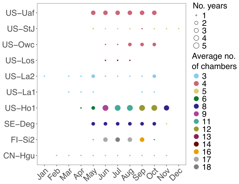
Figure B1 Number of individual chambers and years per month per site. The size of the point describes the number of years and color the average number of individual chambers used within each month across years.

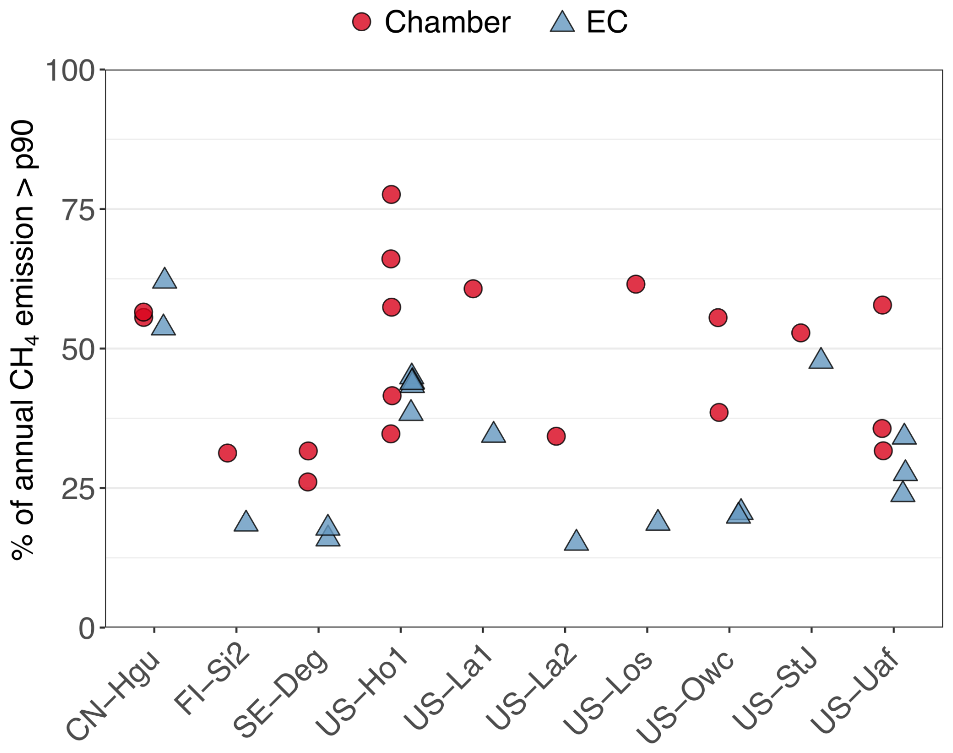
Figure B2 Contribution of high methane (CH₄) emissions to annual CH₄ emissions per site in the unaggregated data set. For each site and year, high CH₄ emissions were estimated as CH₄ flux (FCH₄) above the 90th percentile (p90) and their proportion (%) of the total annual CH₄ emission was calculated separately for chamber (red circle) and EC (blue triangle). In the unaggregated data set, all eddy covariance (EC) FCH₄ data is in the half-hourly scale, but the chamber data measurement frequency varies across sites (see Table S1).

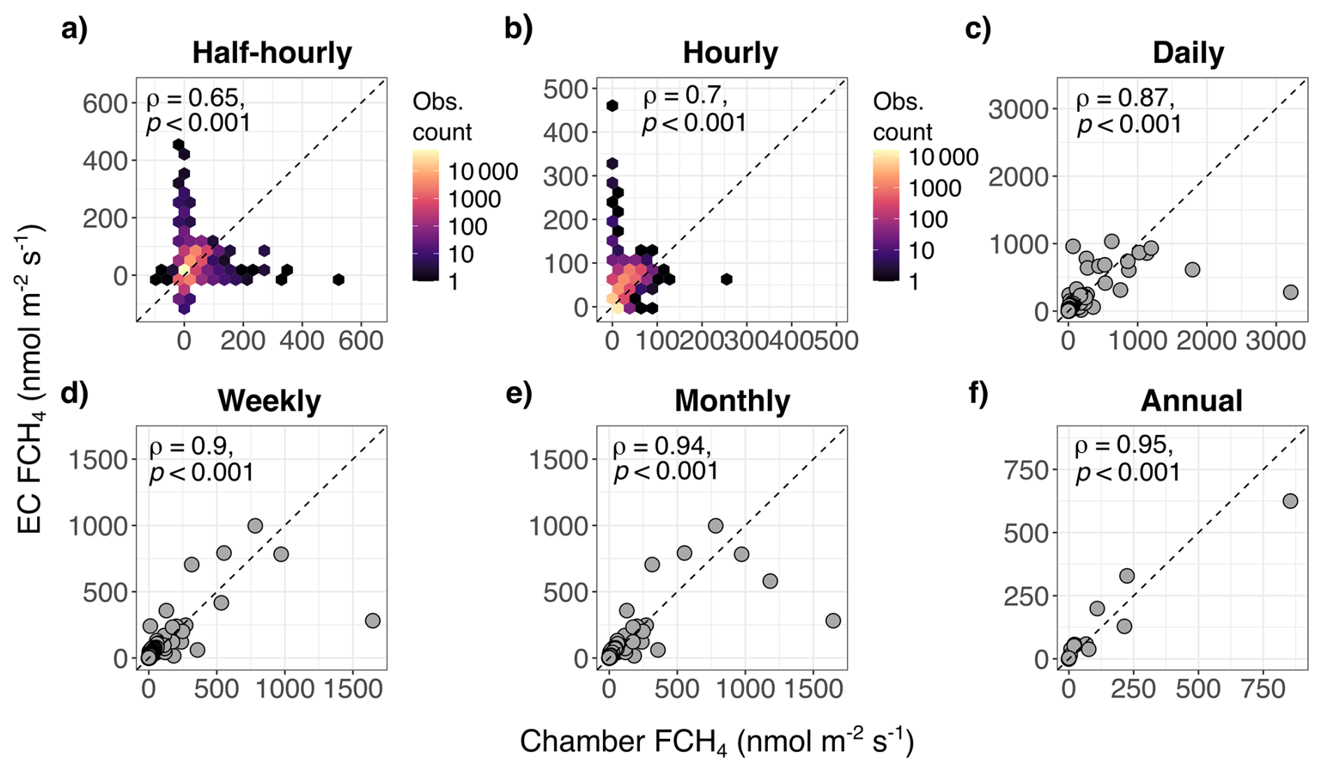
Figure B3 Relationship between eddy covariance (EC; ecosystem scale) methane (CH₄) flux (FCH₄) and chamber FCH₄ (plot scale) with untransformed plot axes. Higher Spearman correlation coefficients (ρ) indicate stronger agreement between EC FCH₄ and chamber FCH₄. In (a) and (b) the points for half-hourly (n=74 482) and hourly (n=40 072) aggregations are shown in hexagonal density clouds with a log-transformed color range to highlight trends in high point density areas (colors represent number of observations per hexagon). For daily (c), weekly (d), monthly (e), and annual (f) aggregations, sample sizes were n=1879, 349, 121, and 22, respectively. The dashed line represents 1:1 line.

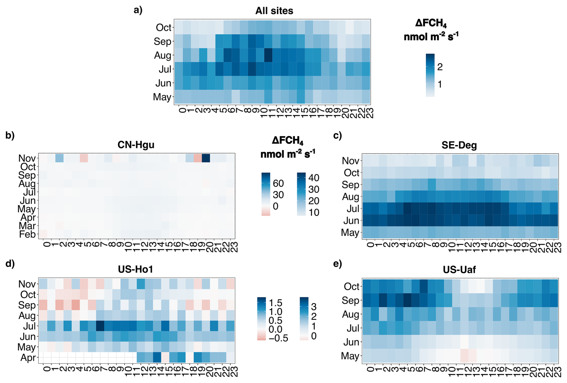
Figure B4 Heatmaps of hourly median methane (CH₄) flux (FCH₄) difference between ecosystem- and plot-scale FCH₄ (ΔFCH₄) across months in the half-hourly aggregation. Positive ΔFCH₄ (blue) represents higher eddy covariance (EC) FCH₄ than chamber FCH₄, and negative (red) higher chamber FCH₄ than EC FCH₄. x axis represents hours of day (24 h) and y axis months. (a) Data set containing all sites (n=4 sites). Only months which were included in all sites are shown (May–October). (b) CN-Hgu (all months), (c) SE-Deg (all months), (d) US-Ho1 (all months), (e) US-Uaf (all months).

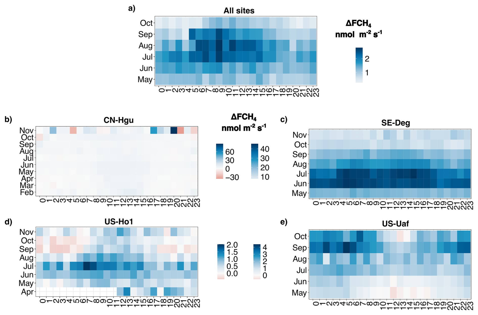
Figure B5 Heatmaps of hourly median methane (CH₄) flux (FCH₄) difference between ecosystem- and plot-scale FCH₄ (ΔFCH₄) across months in the hourly aggregation. Positive ΔFCH₄ (blue) represents higher ecosystem-scale (eddy covariance; EC) FCH₄ than plot-scale (chamber) FCH₄, and negative (red) higher plot-scale FCH₄ than ecosystem-scale FCH₄. x axis represents hours of day (24 h) and y axis months. (a) Data set containing all sites (n=4 sites). Only months which were included in all sites are shown (May–October). (b) CN-Hgu (all months), (c) SE-Deg (all months), (d) US-Ho1 (all months), (e) US-Uaf (all months).

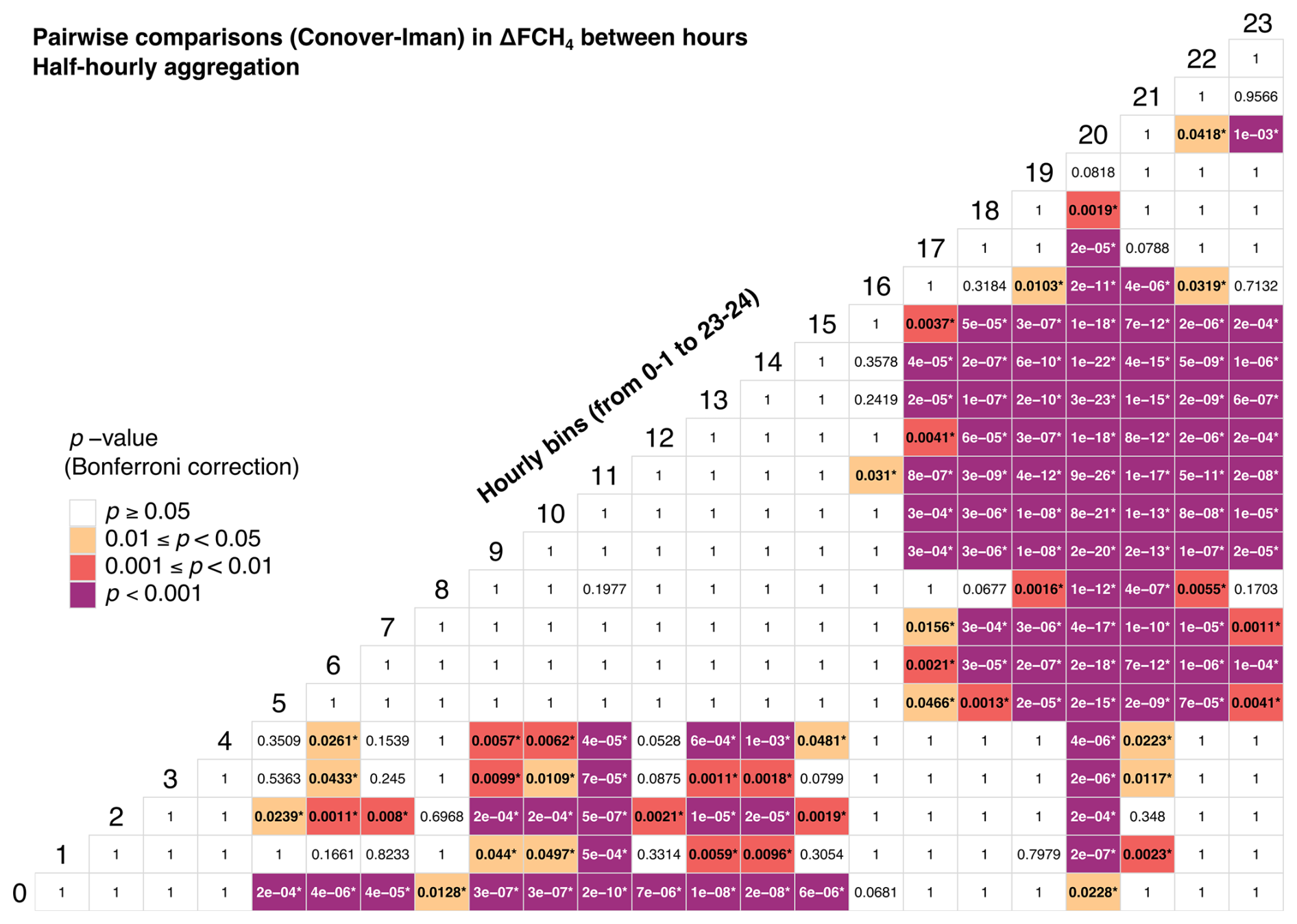
Figure B6 Significance levels (Bonferroni-adjusted p-values) of Conover-Iman multiple pairwise comparisons in methane (CH₄) flux (FCH₄) difference (ΔFCH₄) in the half-hourly aggregation containing sites with automated chamber measurements (n=4 sites). Numbers on the diagonal line are labels for the hourly bins, starting from 0–1 and ending in 23–24. Different colors represent the Bonferroni-adjusted p-values, with reference to an overall significance threshold of α=0.05. Numbers inside the tiles are Bonferroni-adjusted p-values of the pairwise comparisons at four decimal places. Values in bold and asterisk (*) represent p-values that remain significant after Bonferroni correction.

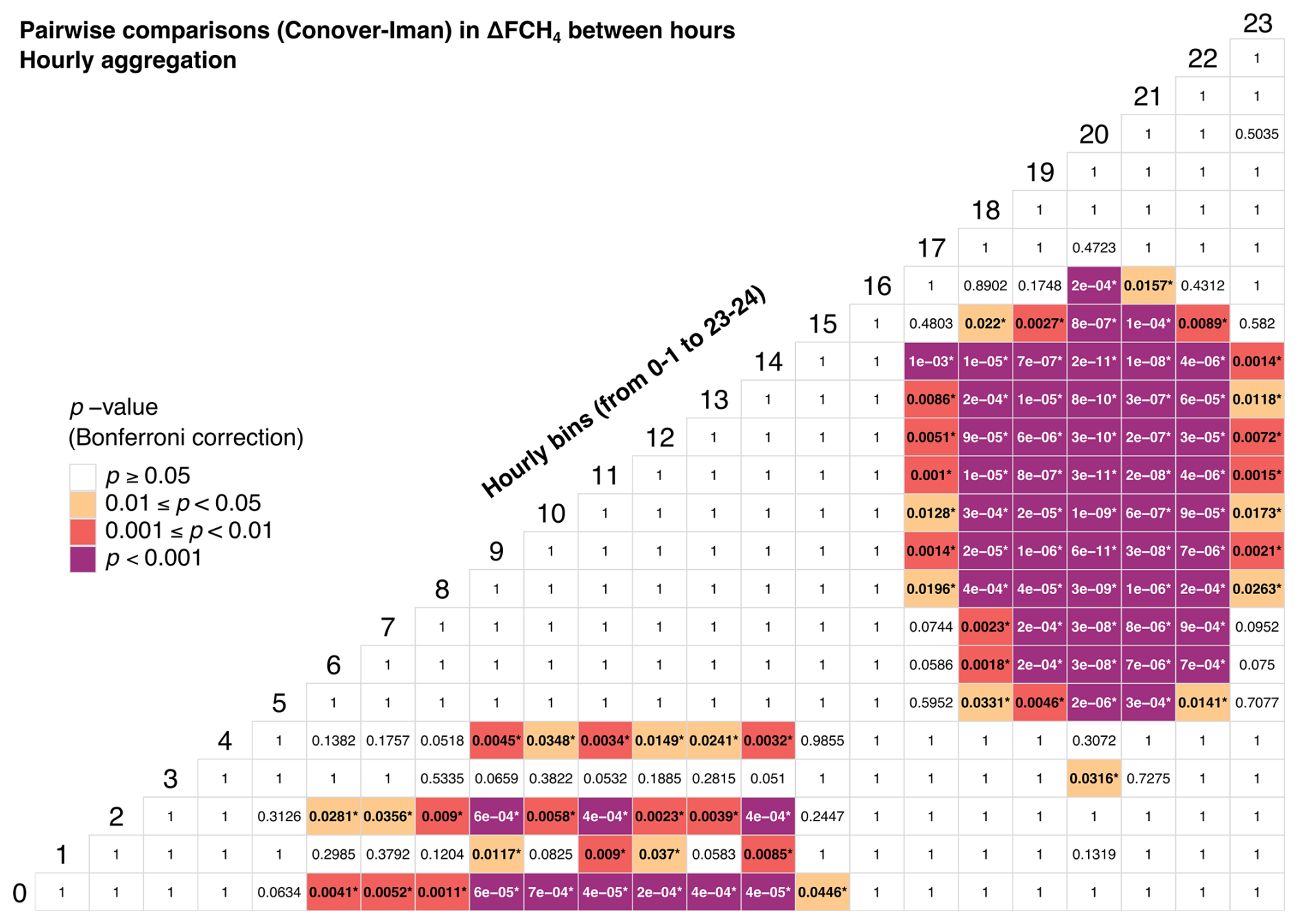
Figure B7 Significance levels (Bonferroni-adjusted p-values) of Conover-Iman multiple pairwise comparisons in methane (CH₄) flux (FCH₄) difference (ΔFCH₄) in the hourly aggregation containing sites with automated chamber measurements (n=4 sites). Numbers on the diagonal line are labels for the hourly bins, starting from 0–1 and ending in 23–24. Different colors represent the Bonferroni-adjusted p-values, with reference to an overall significance threshold of α=0.05. Numbers inside the tiles are Bonferroni-adjusted p-values of the pairwise comparisons at four decimal places. Values in bold and asterisk (*) represent p-values that remain significant after Bonferroni correction.

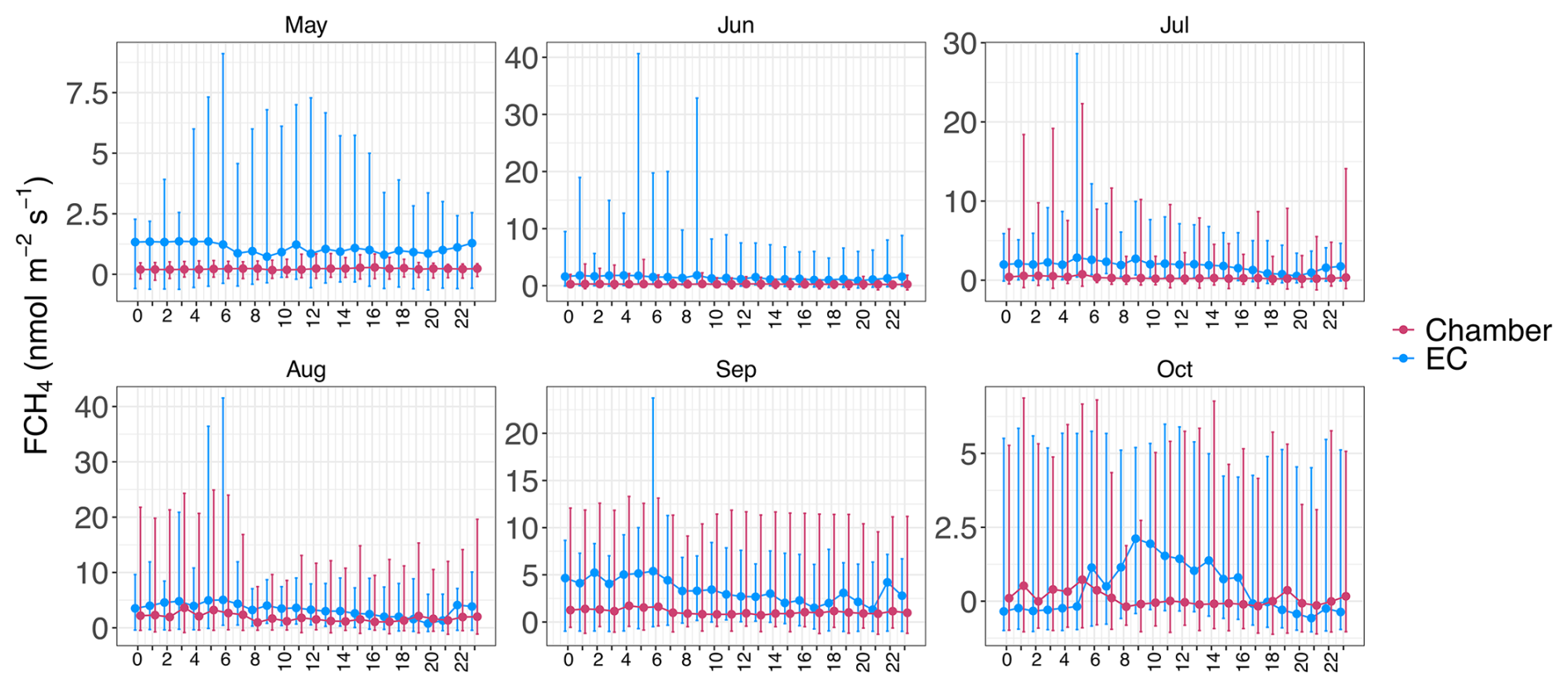
Figure B8 Hourly median chamber (red; plot scale) and eddy covariance (EC; ecosystem scale) methane (CH₄) flux (FCH₄; blue) per month in the half-hourly data set. Variation around the median is represented by the interquartile range (between 25 % and 75 %). Only months containing all sites (n=4) with automated chamber measurements are shown.

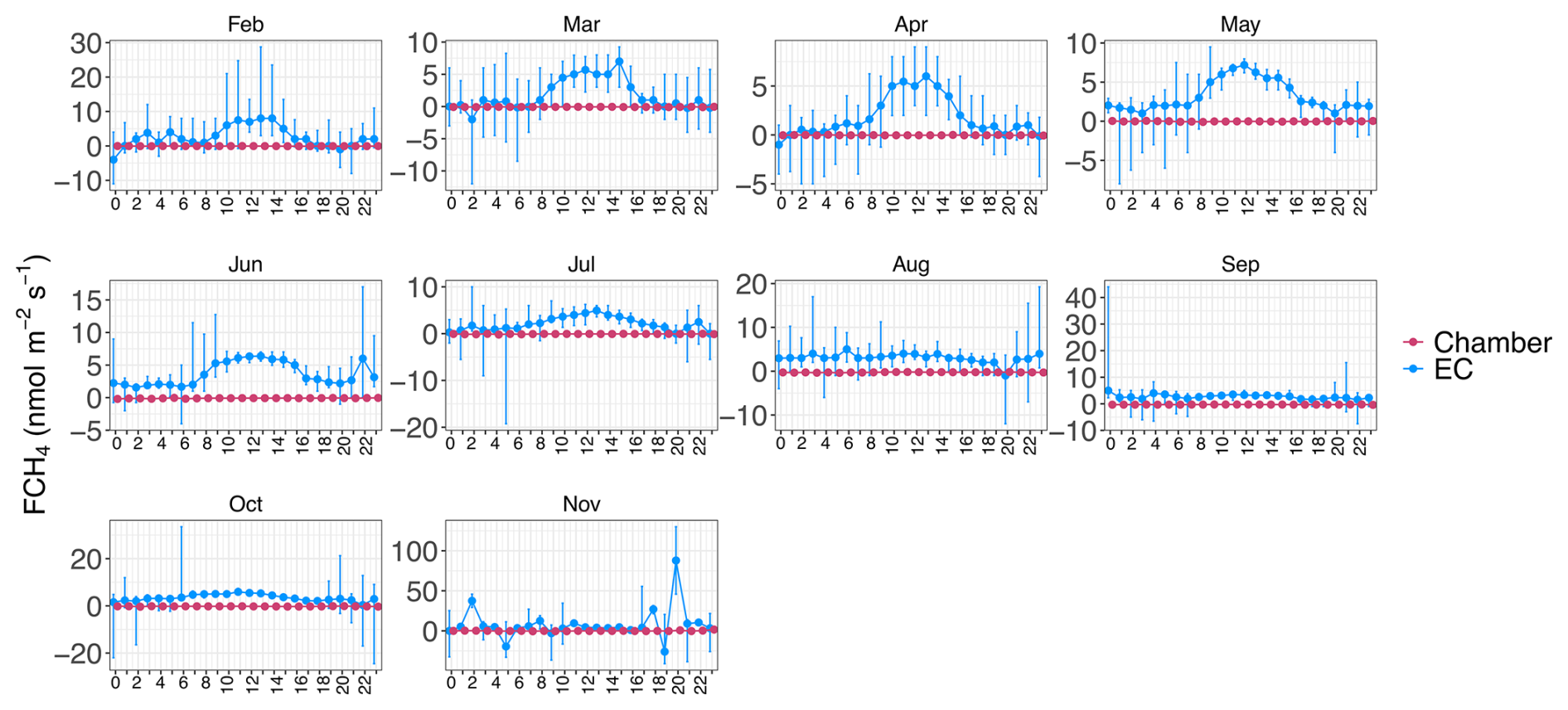
Figure B9 Hourly median chamber (red; plot scale) and eddy covariance (EC; ecosystem scale) methane (CH₄) flux (FCH₄; blue) per month at CN-Hgu in the half-hourly dataset. Variation around the median is represented by the interquartile range (between 25 % and 75 %).

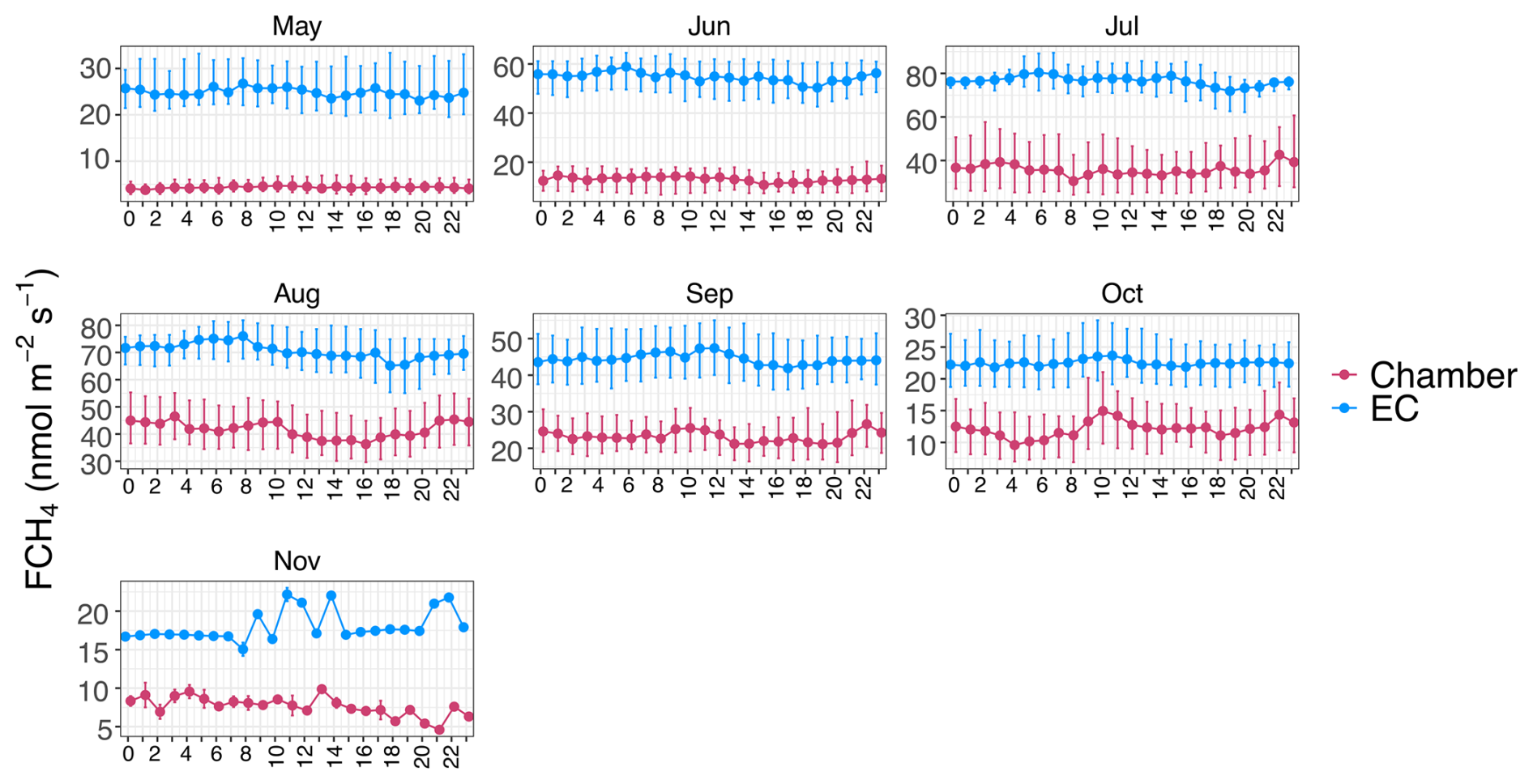
Figure B10 Hourly median chamber (red; plot scale) and eddy covariance (EC; ecosystem scale) methane (CH₄) flux (FCH₄; blue) per month at SE-Deg in the half-hourly dataset. Variation around the median is represented by the interquartile range (between 25 % and 75 %).

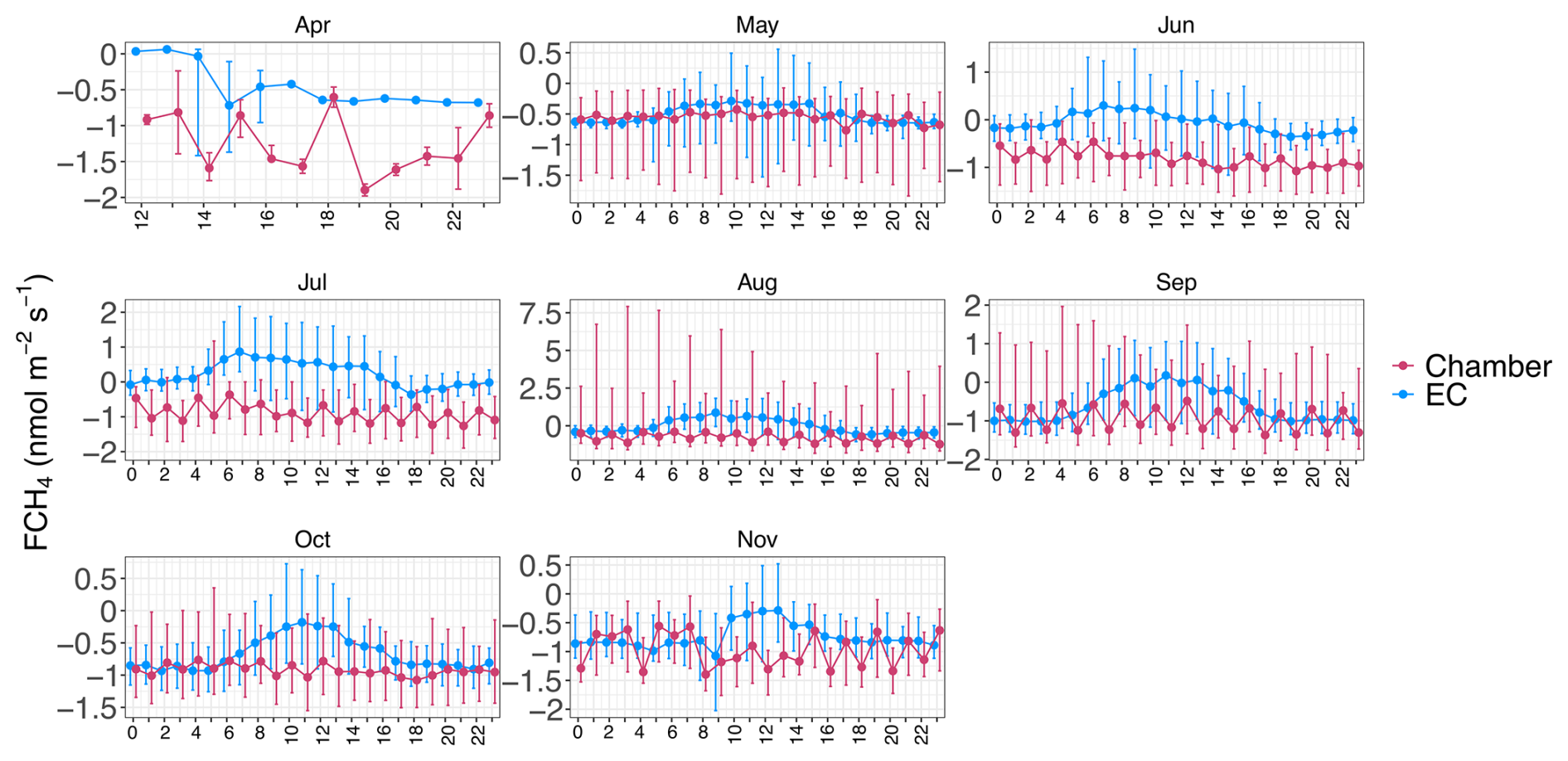
Figure B11 Hourly median chamber (red; plot scale) and eddy covariance (EC; ecosystem scale) methane (CH₄) flux (FCH₄; blue) per month at US-Ho1 in the half-hourly dataset. Variation around the median is represented by the interquartile range (between 25 % and 75 %).

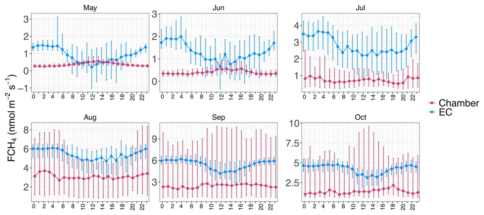
Figure B12 Hourly median chamber (red; plot scale) and eddy covariance (EC; ecosystem scale) methane (CH₄) flux (FCH₄; blue) per month at US-Uaf in the half-hourly dataset. Variation around the median is represented by the interquartile range (between 25 % and 75 %).

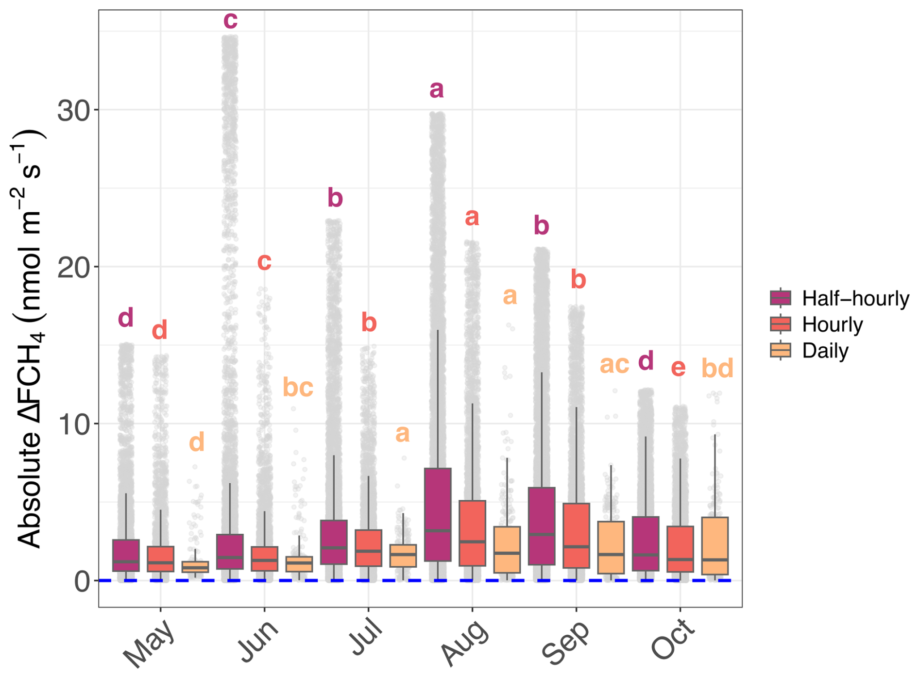
Figure B13 Absolute difference between ecosystem-scale (eddy covariance; EC) and plot-scale (chamber) methane (CH₄) flux (FCH₄) differences (ΔFCH₄) between months in half-hourly, hourly and daily aggregations. Different colors represent different temporal aggregations and gray points show the underlying data. For visualization, we filtered out data points 1.5 × IQR below the first quartile and 1.5 × IQR above the third quartile but statistics were based on the original data. The letters indicate whether ΔFCH₄ differs significantly between months: months that share at least one shared letter are not significantly different (p>0.05) while months with different letters differ significantly (p≤0.05). Pairwise comparisons were conducted with the Conover-Iman post hoc test. While there was data in other months, the May–October period was chosen for this figure due to these months including either all (n=4; half-hourly and hourly aggregations) or almost all sites (n=7 or 8 sites; daily aggregation). Weekly and monthly aggregations did not have significant ΔFCH₄ differences between months (Kruskal-Wallis p>0.05) and are not shown in this figure.

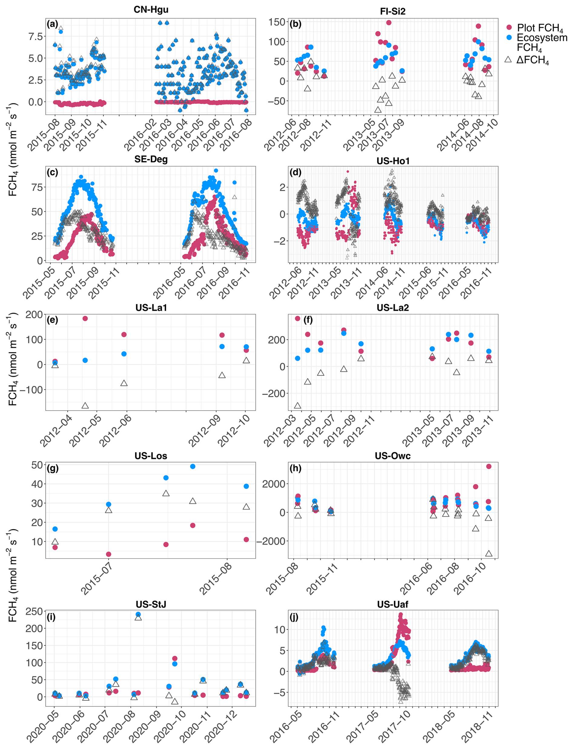
Figure B14 Site-specific trends in daily ecosystem- (eddy covariance; EC) and plot-scale (chamber) methane (CH₄) flux (FCH₄), and FCH₄ difference between ecosystem and plot scales (ΔFCH₄) (a to j). Red circles represent plot- and blue ecosystem-scale FCH₄ measurements. Hollow gray triangles are ΔFCH₄. In (d) 46 outlier points from 2013 were removed to improve visualization. Negative ΔFCH₄ indicates higher plot-scale FCH₄ than ecosystem-scale FCH₄, and positive higher ecosystem-scale FCH₄ than plot-scale FCH₄.

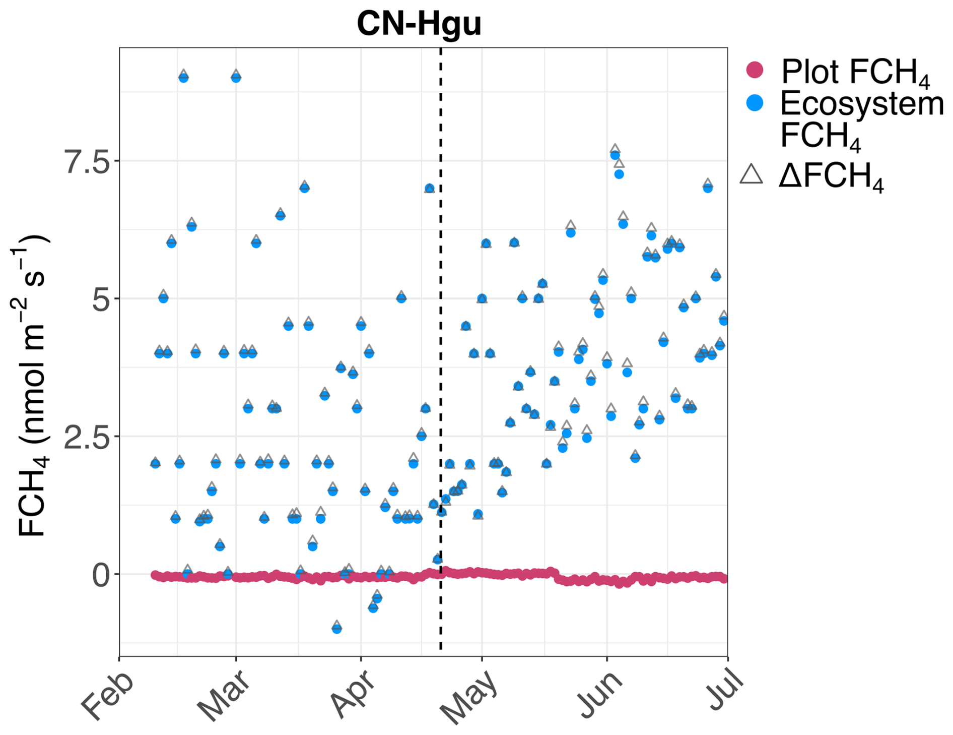
Figure B15 Daily-aggregated methane (CH₄) flux (FCH₄) at CN-Hgu between February and July highlighting the higher ecosystem- than plot-scale FCH₄ during the ice thawing period (February–end of April). Red circles represent plot- and blue ecosystem-scale FCH₄ measurements. Hollow gray triangles are the difference between ecosystem- and plot-scale FCH₄ (ΔFCH₄). Negative ΔFCH₄ indicates higher plot-scale FCH₄ than ecosystem-scale FCH₄, and positive higher ecosystem-scale FCH₄ than plot-scale FCH₄. The dashed vertical black line represents the mean end period of frozen-thawing period at a nearby peatland (between 2015 and 2016), calculated by Liu et al. (2021).

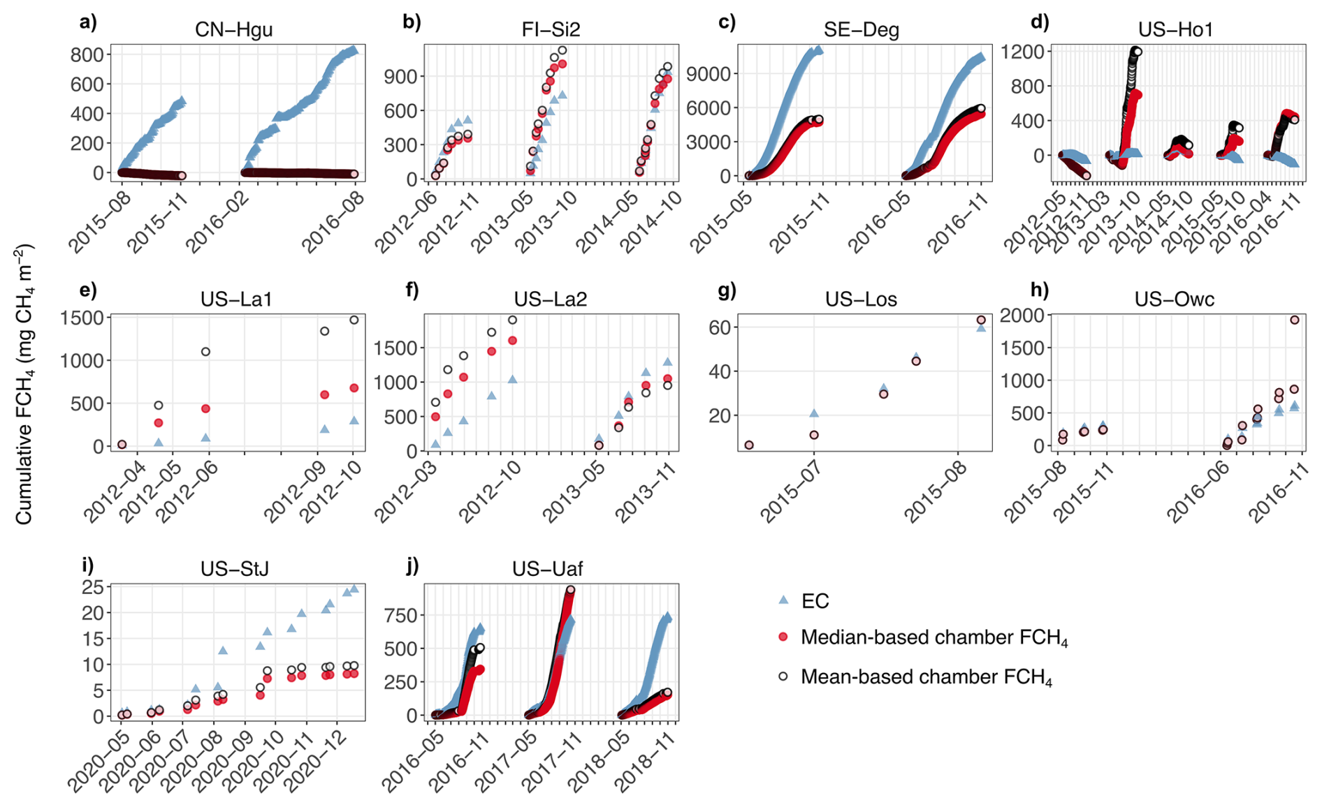
Figure B16 Cumulative sums of ecosystem-scale (eddy covariance; EC) and plot-scale (chamber) methane (CH₄) flux (FCH₄) at the daily scale across sites (a–j). Blue triangles represent EC, red points chamber FCH₄ calculated from the median-based aggregation, and white points chamber FCH₄ calculated from the mean-based aggregation. Note that since the chamber FCH₄ data at FI-Si2, US-La1, and US-La2 lacked hourly timestamps, we roughly estimated daily cumulative FCH₄ by using the daily chamber FCH₄ median or mean for all 24 h of the measurement date (EC cumulative FCH₄ was calculated based on daily half-hourly FCH₄ from FLUXNET-CH₄), and these estimates should thus be interpreted with caution.

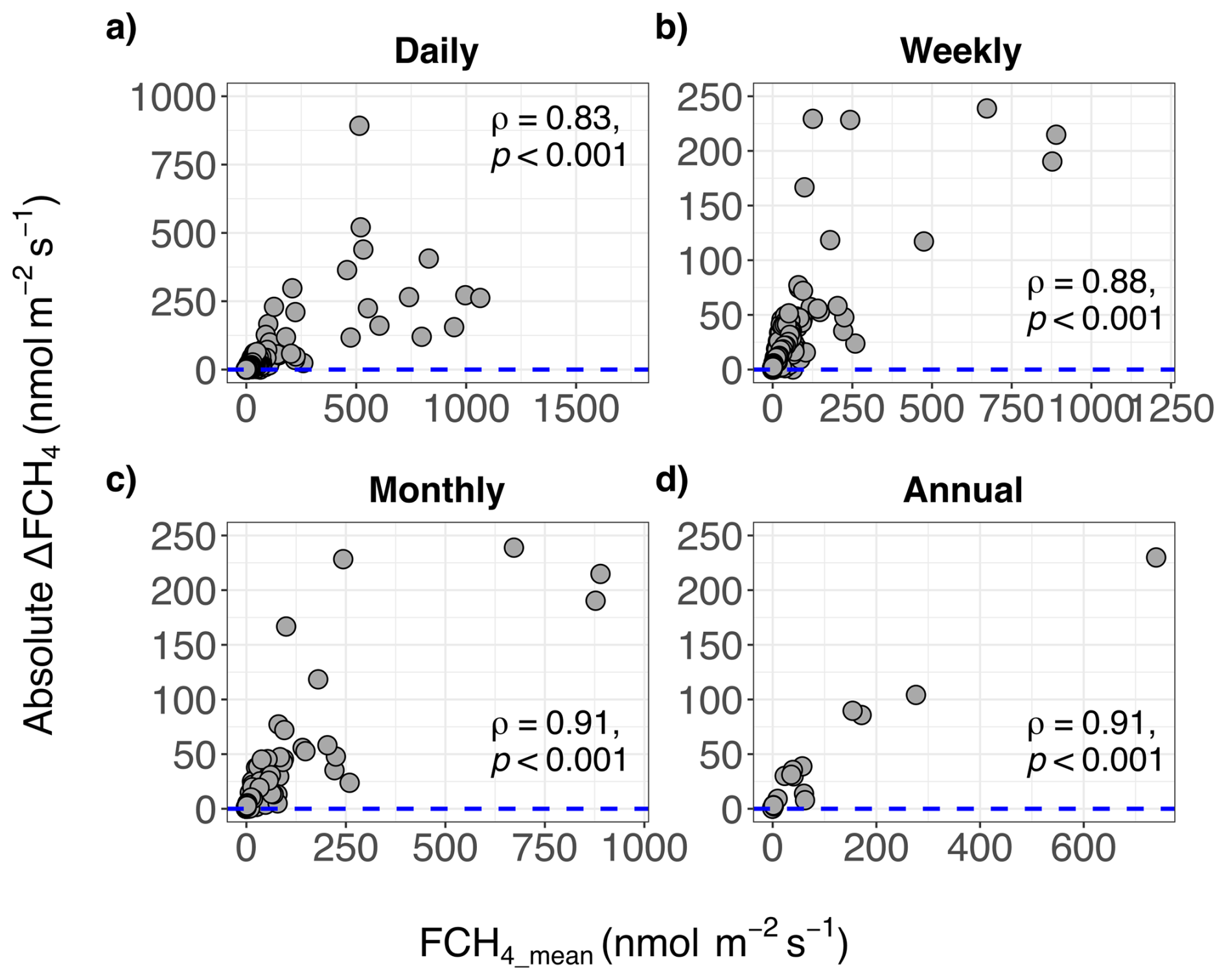
Figure B17 The relationship between methane (CH₄) flux (FCH₄) magnitude and absolute difference between ecosystem- and plot-scale FCH₄ (ΔFCH₄) with outliers in daily (a), weekly (b), monthly (c) and annual (d) scales. FCH_{4_mean} is the row-wise mean of eddy covariance (EC) FCH₄ and chamber FCH₄, and EC-chamber FCH₄ difference (ΔFCH₄) was calculated by subtracting chamber FCH₄ from EC FCH₄. Positive ΔFCH₄ indicates higher EC FCH₄ than chamber FCH₄ and negative values higher chamber FCH₄ than EC FCH₄. The blue dashed line represents the line of equality where EC FCH₄ and chamber FCH₄ are equal. ρ represents Spearman correlation coefficient, followed by its statistical significance (α = 0.05). Higher ρ represents stronger deviation from the line of equality, i.e., ΔFCH₄=0 while perfect agreement between chamber and EC FCH₄ would result in ρ=0.

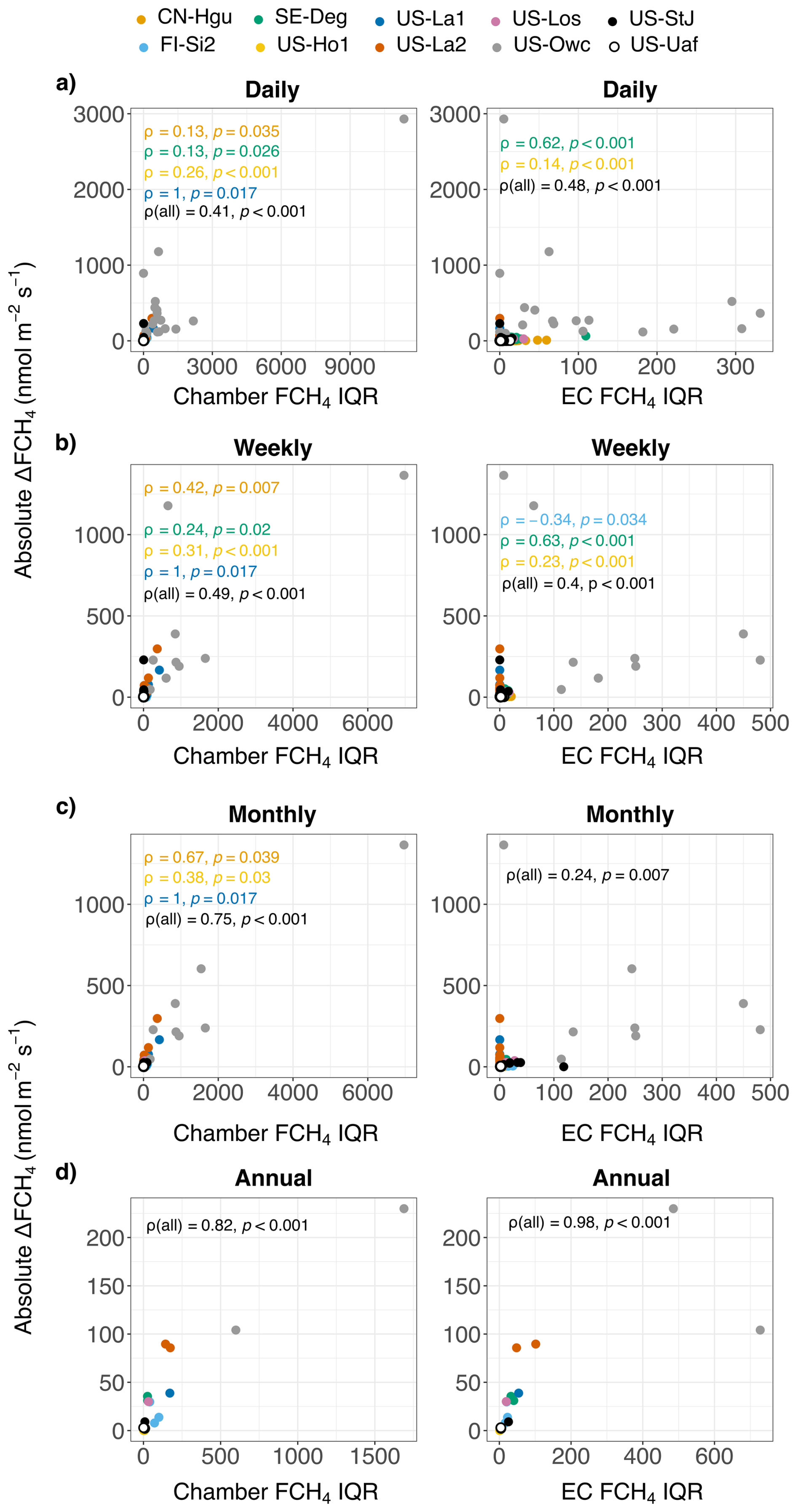
Figure B18 Untransformed absolute difference between ecosystem (eddy covariance; EC)- and plot-scale (chamber) methane (CH₄) flux (FCH₄) (ΔFCH₄), chamber and EC FCH₄ IQR in daily (a), weekly (b), monthly (c), and annual (d) aggregations. Different colors represent individual sites. Plots in the left panel show the relationship between daily variation in FCH₄ between individual chambers within each site and site-level absolute ΔFCH₄. The right side panel shows the same but with daily variation in EC FCH₄. The strength and general direction of the relationship was measured with Spearman correlation coefficient (ρ). “ρ(all)” refers to the Spearman correlation for the whole dataset.

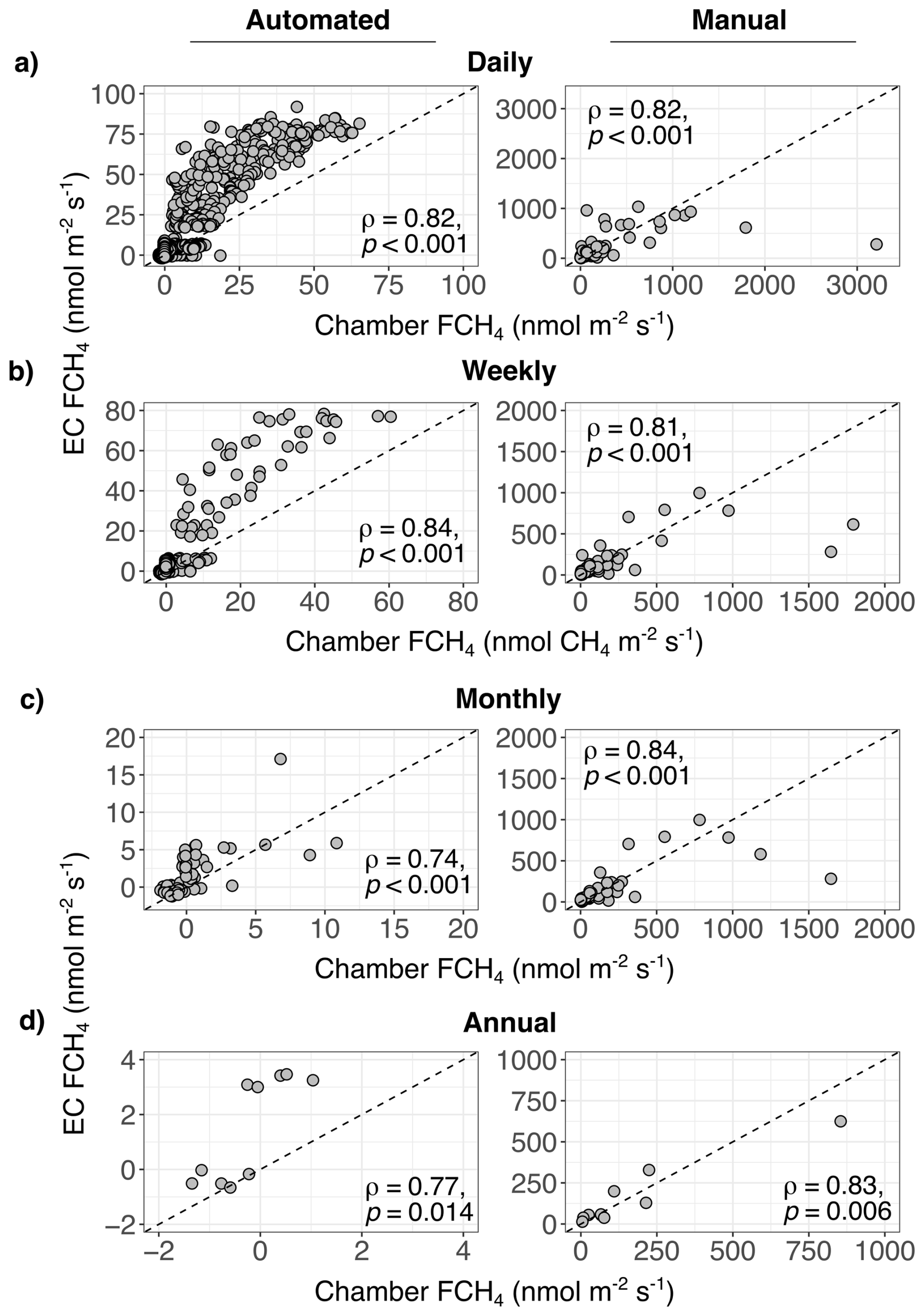
Figure B19 Automated (left panel) and manual (right panel) chamber methane (CH₄) flux (FCH₄) had strong positive relationships with EC FCH₄ across sites and temporal scales (a to d). The dashed line represents the 1:1 line, and ρ Spearman correlation coefficient of the relationship. Automated chambers were included in four sites (CN-Hgu, SE-Deg, US-Ho1, and US-Uaf) and manual chambers in six sites (FI-Si2, US-La1, US-La2, US-Los, US-Owc, and US-StJ). Half-hourly and hourly plots are in Fig. 3. Note different x and y axis scales.

Appendix C: Supplementary tables (Tables C1–C14)

Table C1 Methodological and data details of the site chamber (CH) and eddy covariance (EC) measurement systems. “CH method” refers to whether the chambers are manual or automated, and whether chambers were dark or transparent to sunlight. CH meas. frequency = chamber measurement frequency. CH-EC overlap is the total duration of overlap between chamber and EC measurements in days (note: the measurements are spread out over different seasons and years; see Fig. B1 and Table 1). Gap-filled EC is the percentage of ANN-gap-filled EC methane (CH₄) flux (FCH₄) values of all EC FCH₄ values per site (in the unaggregated data set). Further details of the CH and EC measurement systems can be found in the corresponding references. Abbreviations in “CH analyzer”: LI-COR = LI-COR Biosciences, Nebraska, USA; Picarro = Picarro Inc., Santa Clara, CA, USA; Los Gatos = Los Gatos Research Inc., San Jose, CA, USA; Aerodyne = TILDAS CS, Aerodyne Research Inc., Billerica, MA, USA; Varian = Varian, Inc., Palo Alto, CA, USA; Shimadzu = Shimadzu Scientific Instruments, Kyoto, Japan.

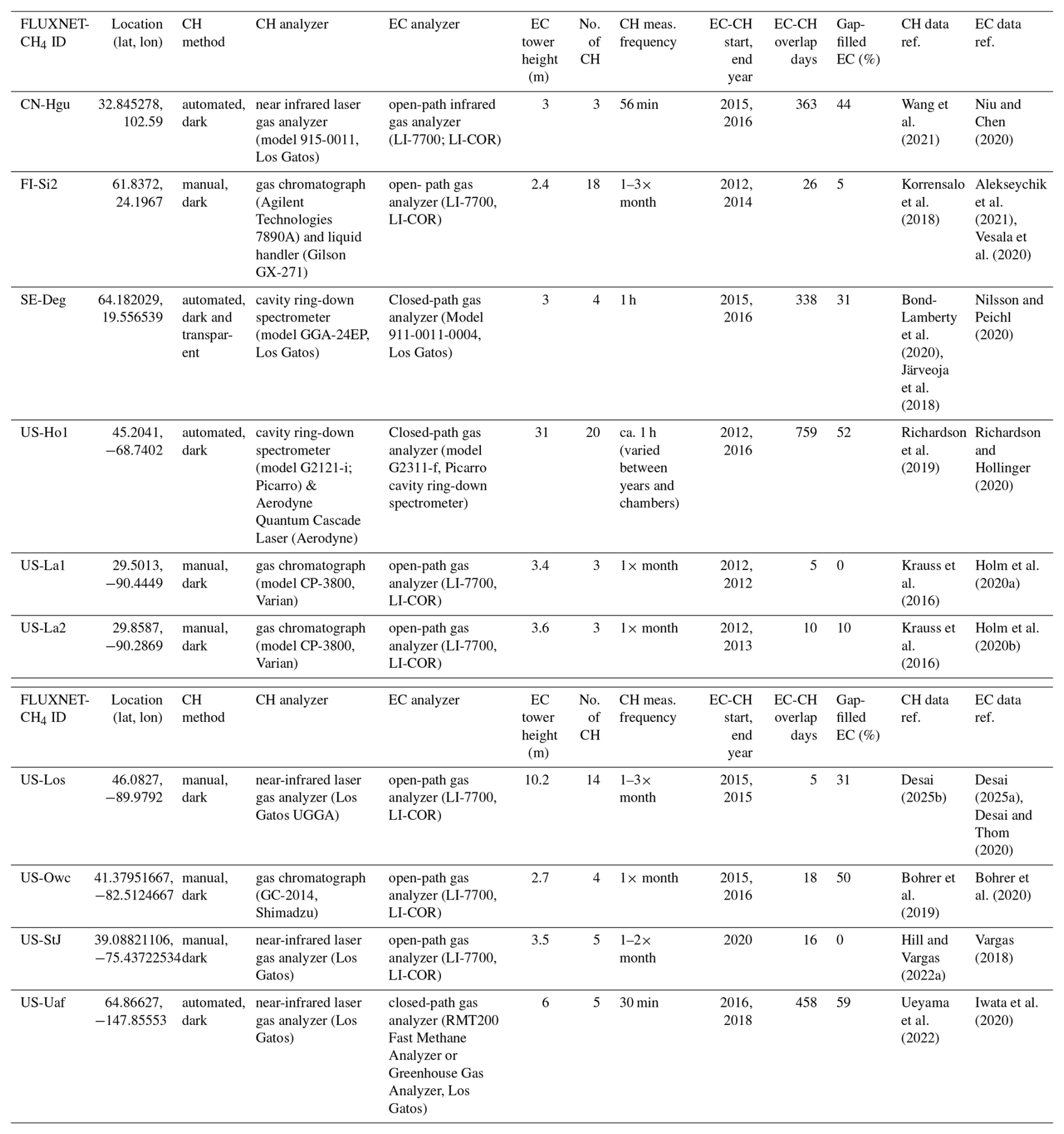
Table C2 Details of chamber methane (CH₄) flux (FCH₄) data quality control and chamber placement rationale in the study sites. Data quality control was done by data providers prior to sharing chamber FCH₄ data, and a summary of the methods are listed here. For more details, please see the site-specific references. EC = eddy covariance.

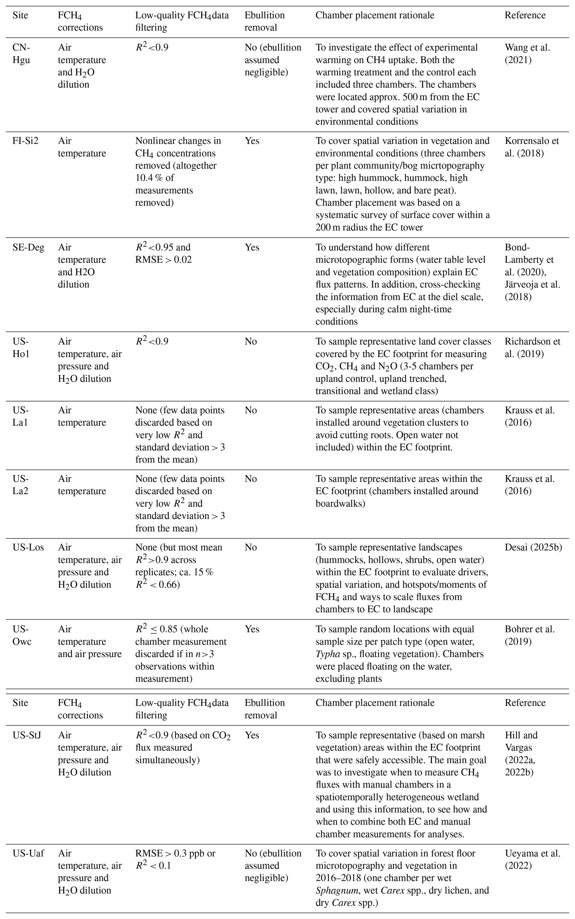
Table C3 Details of the used environmental data. FLUXNET-CH₄ soil temperature data was from the topmost soil depths (2-10 cm below soil surface). Abbreviations: NEE = net ecosystem exchange, u^* = friction velocity, WD = wind direction, WS = wind speed, VPD = vapor pressure deficit, PA = air pressure, WTL = water table level, TS = soil temperature, ANN = artificial neural network, MDS = marginal distribution sampling.

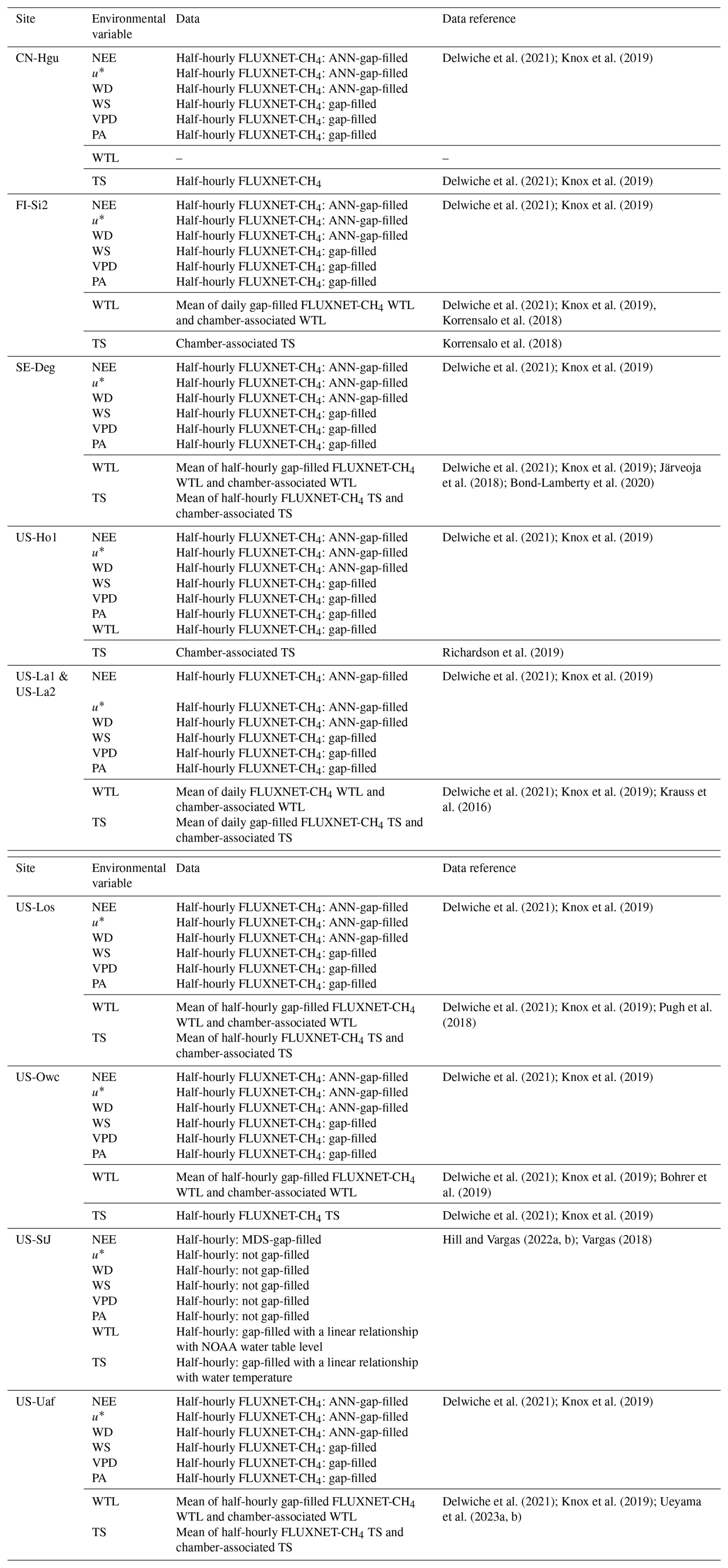
Table C4 Descriptive statistics and Wilcoxon-Mann-Whitney test results based on temporal aggregations from chamber and eddy covariance (EC) methane (CH₄) flux (FCH₄) means instead of medians. Proportions of annual chamber and EC CH₄ emission (i.e., FCH₄ ≤ 0 excluded) above the 90th percentile (p90) are reported to highlight the contribution of high CH₄ emission values to FCH₄. Abbreviations: IQR = interquartile range, SD = standard deviation, CV = coefficient of variation (%), EC = eddy covariance.

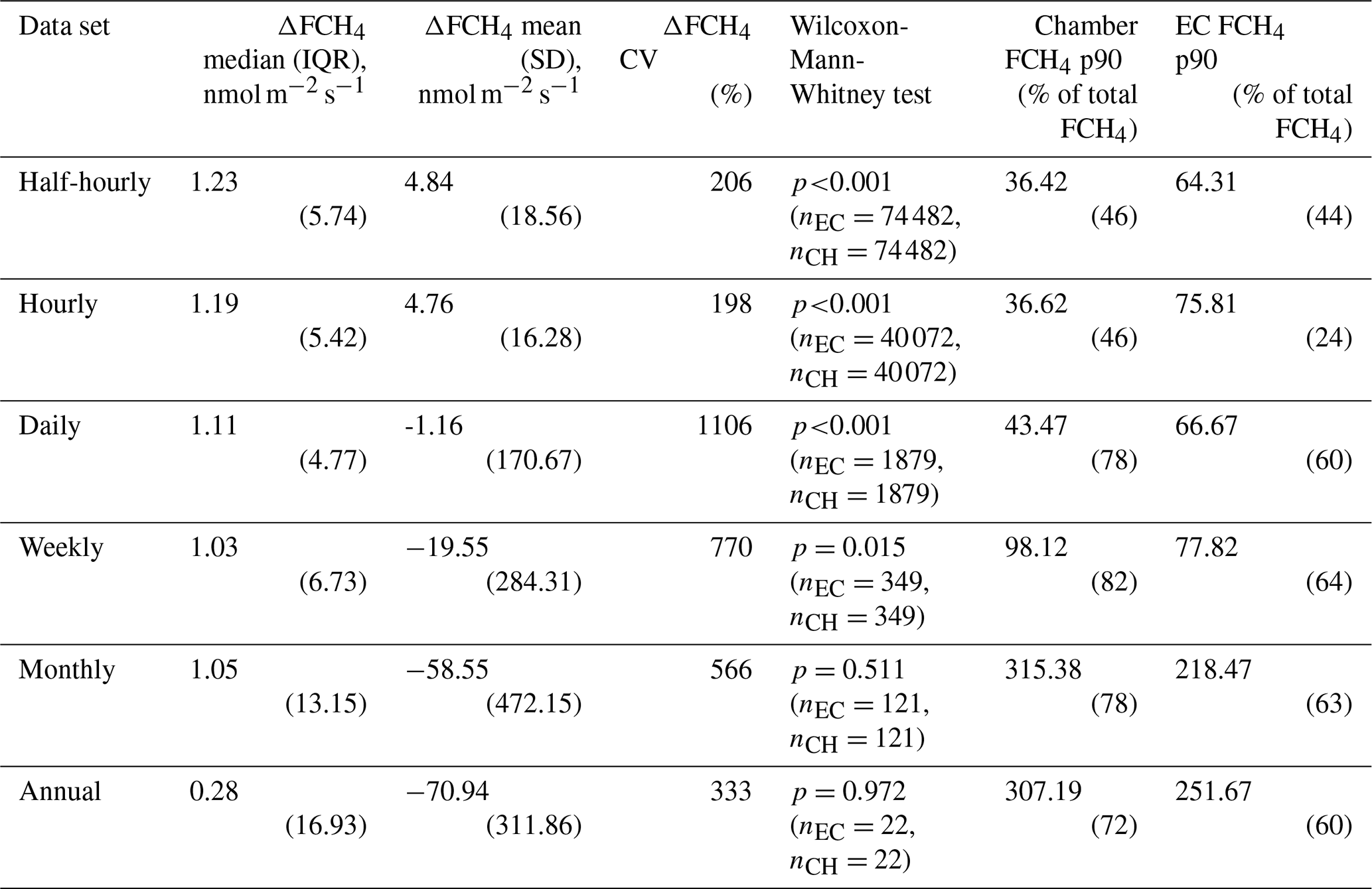
Table C5 Descriptive statistics and Wilcoxon-Mann-Whitney test results for the difference between ecosystem- and plot-scale methane (CH₄) flux (FCH₄) (ΔFCH₄) based on cumulative eddy covariance (EC) and chamber FCH₄ (mg CH₄ m⁻²) at daily to annual aggregations (note: cumulative FCH₄ were calculated only for exact EC-chamber FCH₄ timestamps and do not represent cumulative sums for ecosystem CH₄ budget calculations). Due to a lack of hourly timestamps in the chamber FCH₄ data at FI-Si2, US-La1 and US-La2, these three sites were excluded from this table, resulting in n=7 sites. Results are given separately for data sets based on median (left) and mean (right) aggregations of chamber and EC FCH₄ at each temporal scale. The EC and chamber data sample sizes in Wilcoxon-Mann-Whitney tests are reported as n_EC and n_CH, respectively. Abbreviations: IQR = interquartile range, SD = standard deviation, CV = coefficient of variation (%).

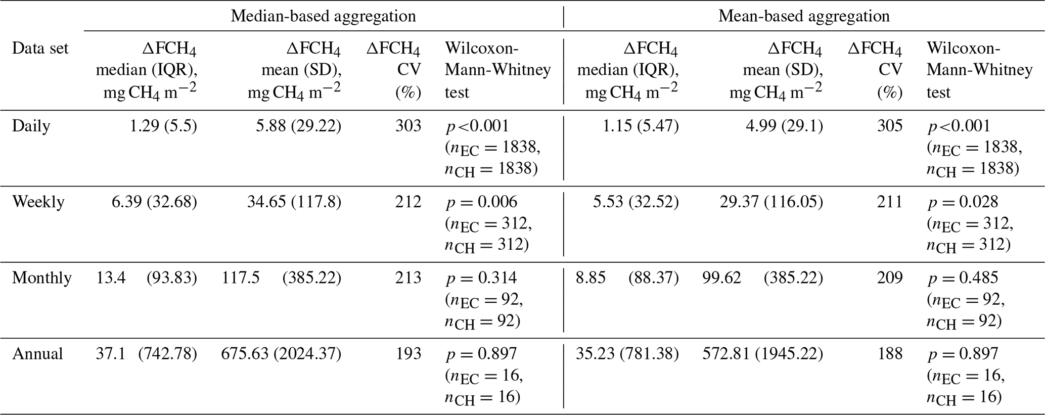
Table C6 Linear mixed effects model results for assessing the slopes between ecosystem-scale (eddy covariance; EC) methane (CH₄) flux (FCH₄) and plot-scale (chamber) FCH₄. To meet residual normality assumptions of linear mixed models, EC FCH₄ was transformed with inverse hyperbolic sine (IHS) and the fixed effect estimates, p-values and standard errors (SE) are in transformed scale. Average marginal effects (AME) and their 95 % confidence intervals (CI) are reported in the back-transformed units (nmol m⁻² s⁻¹) and represent the average change in EC FCH₄ with a 1 nmol m⁻² s⁻¹ increase in chamber FCH₄ across all chamber FCH₄ observations. AME CIs were obtained with parametric simulation from the fixed effect estimate and covariance. Half-hourly and hourly models are not included due to non-convergence and residual non-normality.

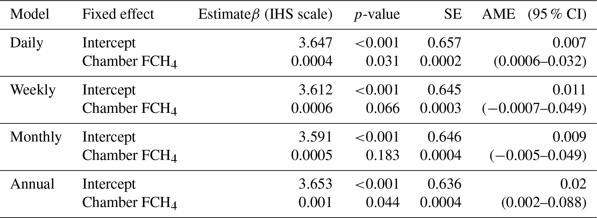
Table C7 Wilcoxon-Mann-Whitney test results for half-hourly aggregation. The eddy covariance (EC) and chamber data sample sizes in Wilcoxon Mann-Whitney tests are reported as n_EC and n_CH, respectively. Proportions of annual chamber and EC methane (CH₄) emission (i.e., CH₄ flux (FCH₄) ≤ 0 excluded) above the 90th percentile (p90) are reported as the mean of year-specific 90th percentiles (not in parentheses) and percentages (in parentheses). This data set contains chamber measurements only from automated chambers (n=4 sites). Abbreviations: IQR = interquartile range, CV = coefficient of variation (%).

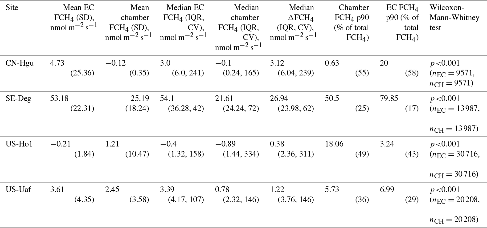
Table C8 Wilcoxon-Mann-Whitney test results for hourly aggregation. The eddy covariance (EC) and chamber data sample sizes in Wilcoxon Mann-Whitney tests are reported as n_EC and n_CH, respectively. Proportions of annual chamber and EC methane (CH₄) emission (i.e., CH₄ flux (FCH₄) ≤ 0 excluded) above the 90th percentile (p90) are reported as the mean of year-specific 90th percentiles (not in parentheses) and percentages (in parentheses). This data set contains chamber measurements only from automated chambers (n=4 sites). Abbreviations: IQR = interquartile range, CV = coefficient of variation (%).

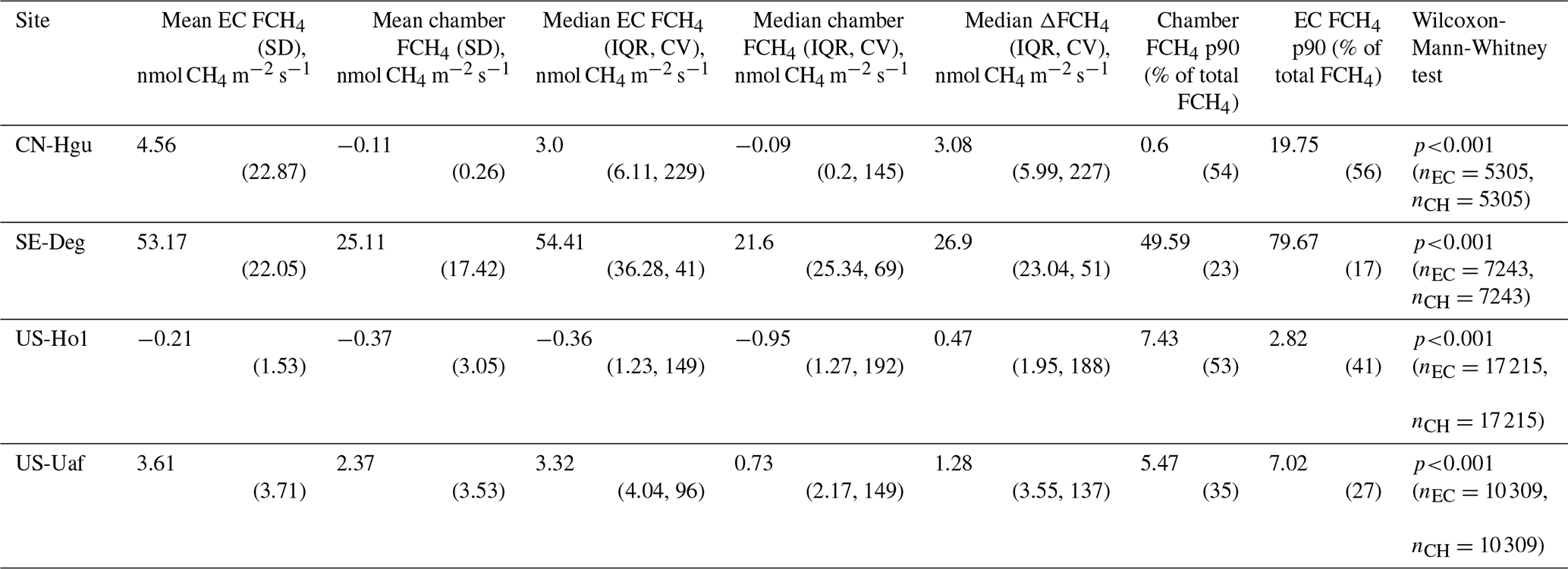
Table C9 Wilcoxon-Mann-Whitney test results for daily aggregation. The eddy covariance (EC) and chamber data sample sizes in Wilcoxon-Mann-Whitney tests are reported as n_EC and n_CH, respectively. Proportions of annual chamber and EC CH₄ emission (i.e., CH₄ flux (FCH₄) ≤ 0 excluded) above the 90th percentile (p90) are reported as the mean of year-specific 90th percentiles (not in parentheses) and percentages (in parentheses). This dataset contains all sites (n=10). Note: due to small sample sizes (n=5) in US-La1 and US-Los, the Wilcoxon-Mann-Whitney test results should be interpreted with caution. Abbreviations: IQR = interquartile range, CV = coefficient of variation (%).

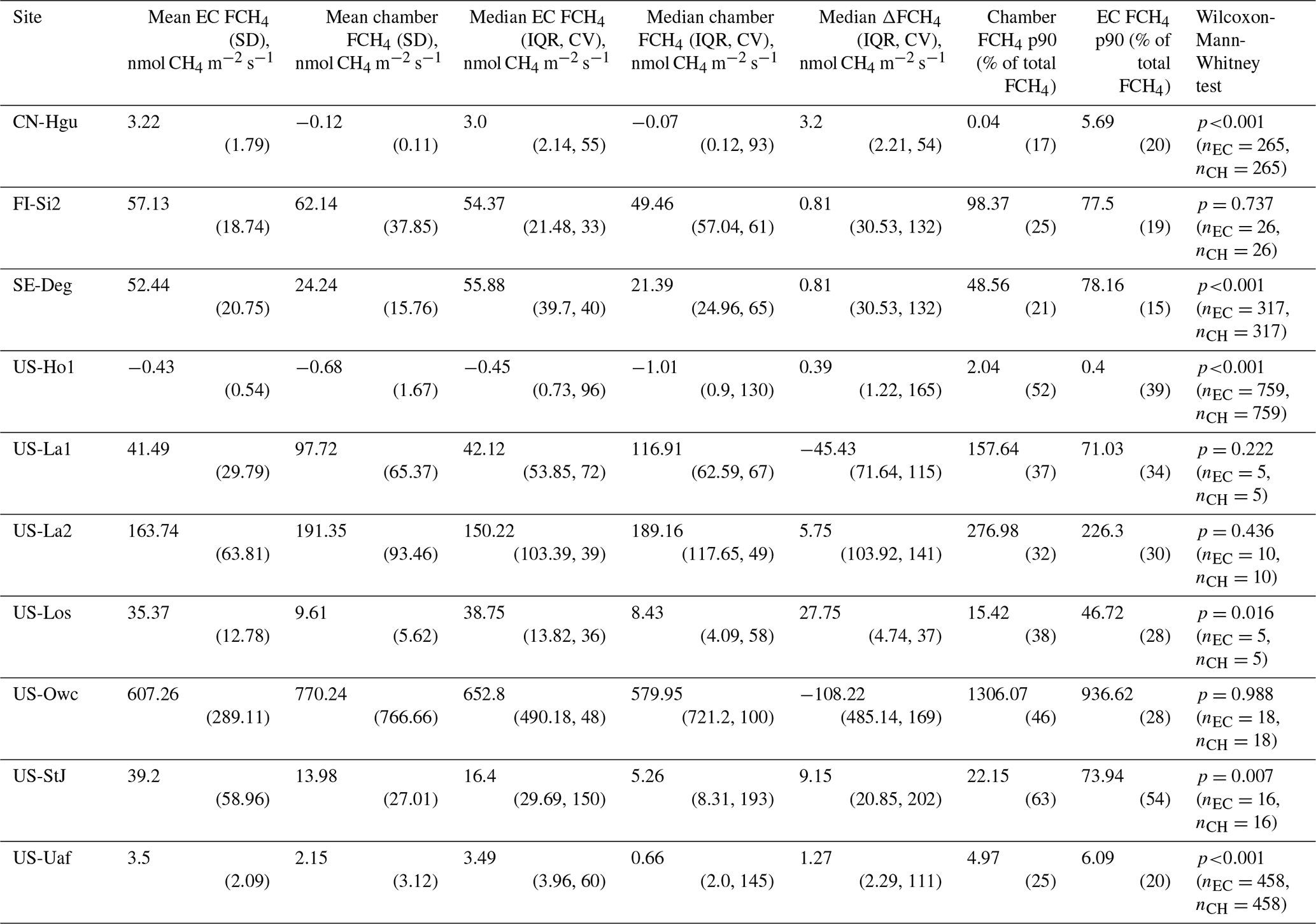
Table C10 Wilcoxon-Mann-Whitney test results for weekly aggregation. The eddy covariance (EC) and chamber data sample sizes in Wilcoxon-Mann-Whitney tests are reported as n_EC and n_CH, respectively. Proportions of annual chamber and EC methane (CH₄) emission (i.e., CH₄ flux (FCH₄) ≤ 0 excluded) above the 90th percentile (p90) are reported as the mean of year-specific 90th percentiles (not in parentheses) and percentages (in parentheses). This dataset contains all sites (n=10). Note: due to small sample sizes (n=5) in US-La1 and US-Los, the Wilcoxon-Mann-Whitney test results should be interpreted with caution. Abbreviations: IQR = interquartile range, CV = coefficient of variation (%).

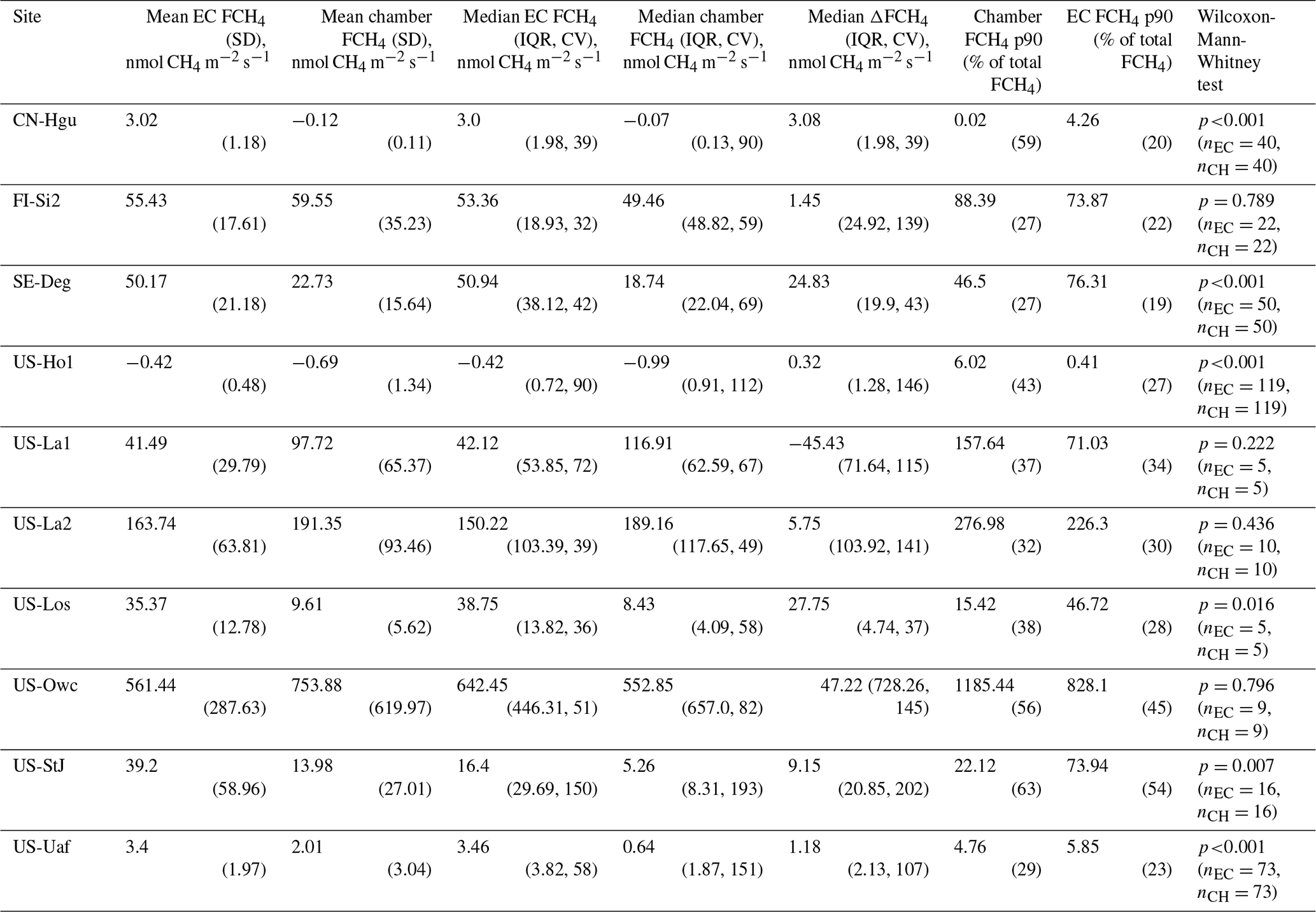
Table C11 Wilcoxon-Mann-Whitney test results for monthly aggregation. The eddy covariance (EC) and chamber data sample sizes in Wilcoxon-Mann-Whitney tests are reported as n_EC and n_CH, respectively. Proportions of annual chamber and EC methane (CH₄) emission (i.e., CH₄ flux (FCH₄) ≤ 0 excluded) above the 90th percentile (p90) are reported as the mean of year-specific 90th percentiles (not in parentheses) and percentages (in parentheses). This dataset contains all sites (n=10). Note: due to small sample sizes (n=5) in US-La1 and US-Los, the Wilcoxon-Mann-Whitney test results should be interpreted with caution. Abbreviations: IQR = interquartile range, CV = coefficient of variation (%). * CN-Hgu had only negative chamber FCH₄ values and chamber p90 was not calculated for this site.

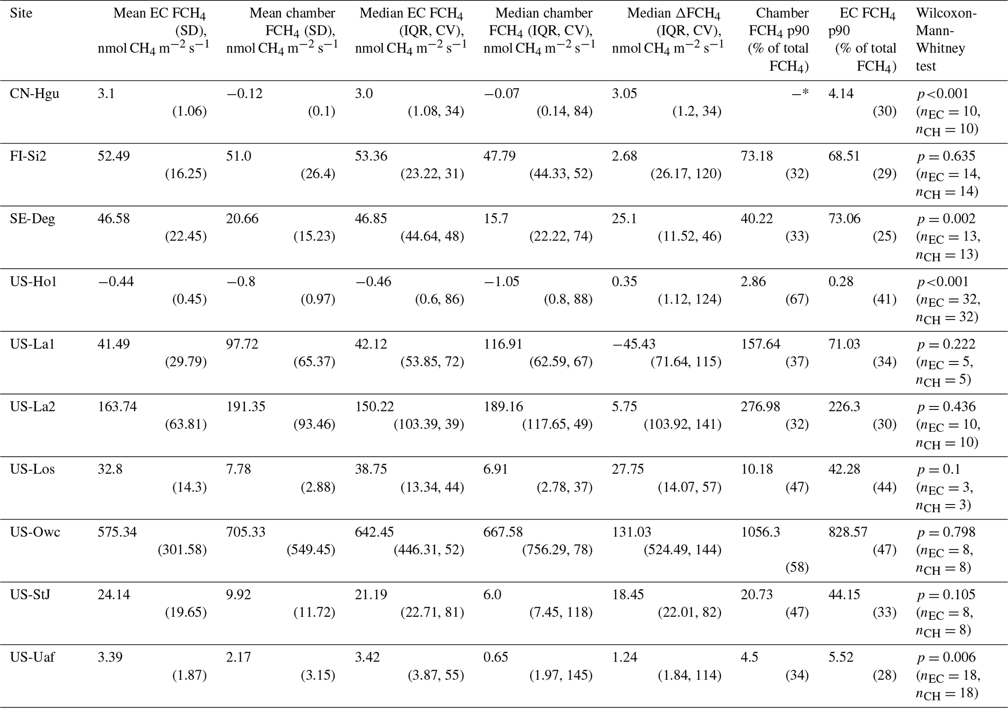
Table C12 Wilcoxon-Mann-Whitney test results for annual aggregation. The eddy covariance (EC) and chamber data sample sizes in Wilcoxon-Mann-Whitney tests are reported as n_EC and n_CH, respectively. Annual chamber and EC methane (CH₄) flux (FCH₄) 90th percentiles were not calculated for this aggregation. This dataset contains all sites (n=10). Note: due to small sample sizes (n=5) in US-La1 and US-Los, the Wilcoxon-Mann-Whitney test results should be interpreted with caution. Abbreviations: IQR = interquartile range, CV = coefficient of variation (%).

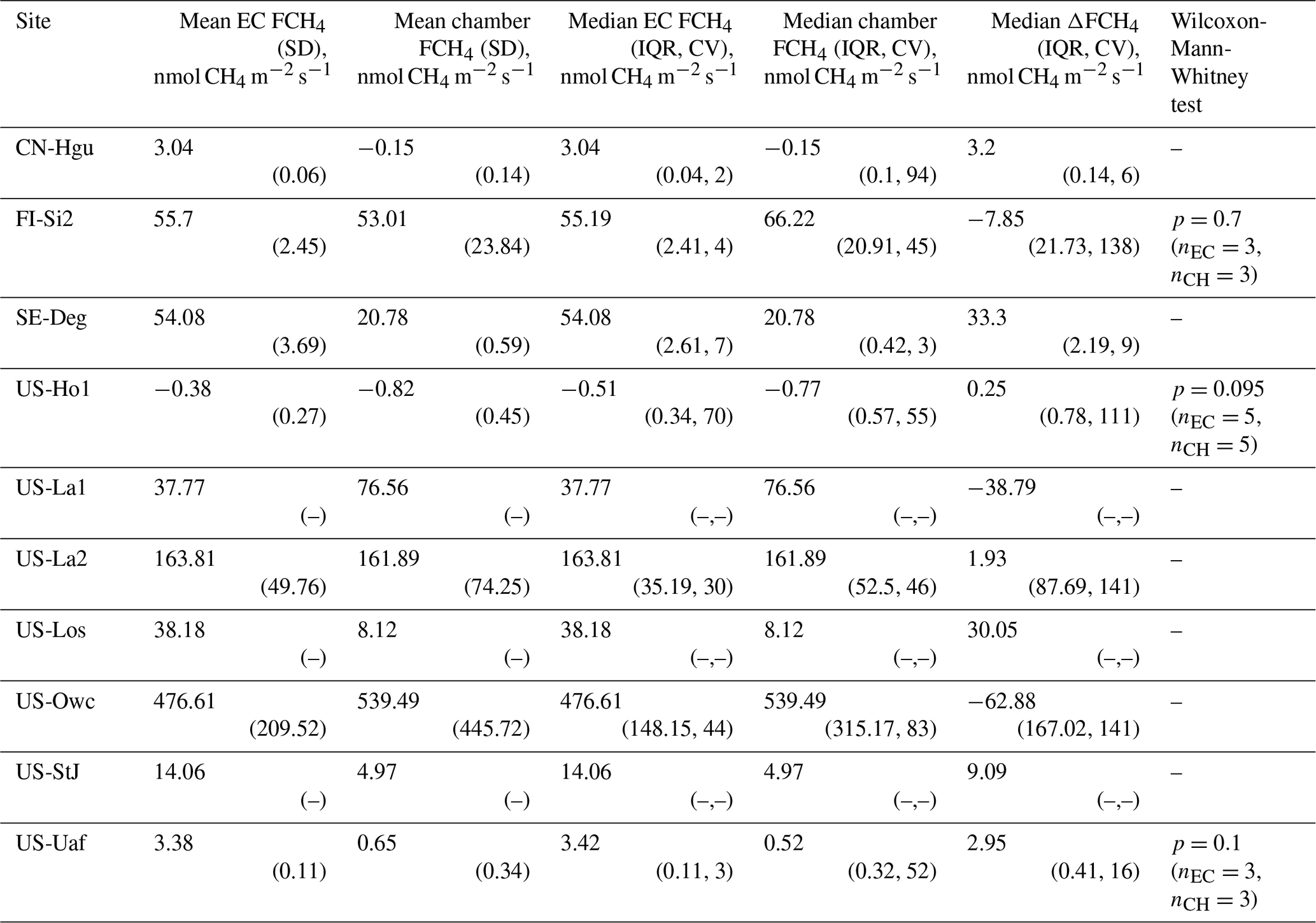
Table C13 Final linear mixed effects model results of significant predictors of the difference between ecosystem- and plot-scale methane (CH₄) flux (FCH₄) (ΔFCH₄) for the half-hourly model (site n=3) with soil temperature (TS) instead of Month as one of the predictors. Absolute ΔFCH₄ was Yeo-Johnson-transformed, centered and scaled, while all continuous predictors were only centered and scaled. The predictors are listed in decreasing order based on β-coefficients. The reference level in Hour was 0 and May in Month. Abbreviations: SE = standard error, Df = degrees of freedom of denominator, LOOCV = leave-one-out cross validation, MAE = mean absolute error, RMSE = root mean square error, PA = air pressure (kPa), u^* = friction velocity (m s⁻¹), WTL = water table level (cm), TS = soil temperature (°C), NEE = net ecosystem exchange (µmol CO₂ m⁻² s⁻¹), VPD = vapor pressure deficit (hPa), vWD = v wind component (m s⁻¹), uWD = u wind component (m s⁻¹). Significant predictors are highlighted in bold.

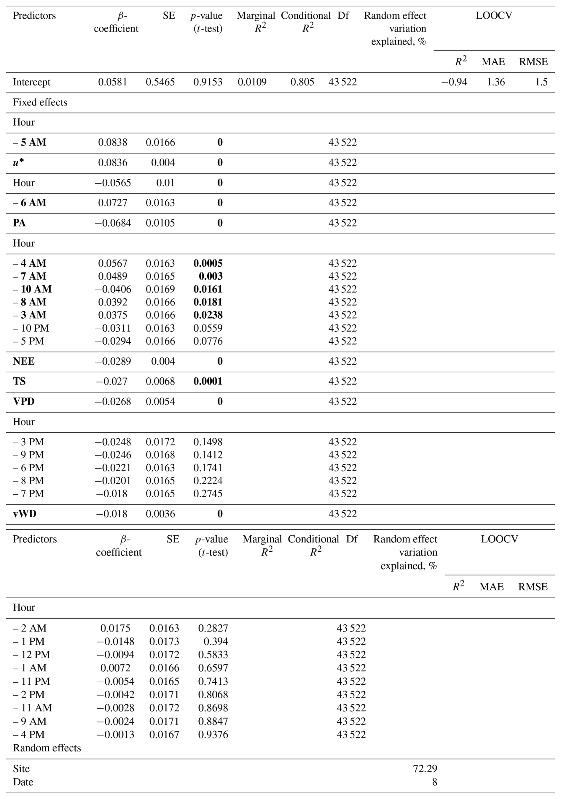
Table C14 Half-hourly and hourly linear mixed effects model results after backward variable selection. In the models, absolute the difference between ecosystem- and plot-scale methane (CH₄) flux (FCH₄) (ΔFCH₄) was Yeo-Johnson-transformed, centered and scaled, while all continuous predictors were only centered and scaled. Note that in both models temporal variables were included in nested random effects (see Supplementary Methods A2). In both models, the reference level in dominant vegetation type was Sphagnum moss, 0 in Hour and May in Month. Note that we excluded TS from the half-hourly model due to high multicollinearity with Month (VIF > 3; see models with TS instead of Month in S17). The predictors are listed in a decreasing order according to their ??-coefficients. SE = standard error, Df = degrees of freedom of denominator, LOOCV = leave-one-out cross validation, MAE = mean absolute error, RMSE = root mean square error, PA = air pressure (kPa), u^* = friction velocity (m s⁻¹), WTL = water table level (cm), TS = soil temperature (°C), NEE = net ecosystem exchange (µmol CO₂ m⁻² s⁻¹), VPD = vapor pressure deficit (hPa), vWD =  v wind component (m s⁻¹), uWD = u wind component (m s⁻¹). Significant predictors are highlighted in bold.

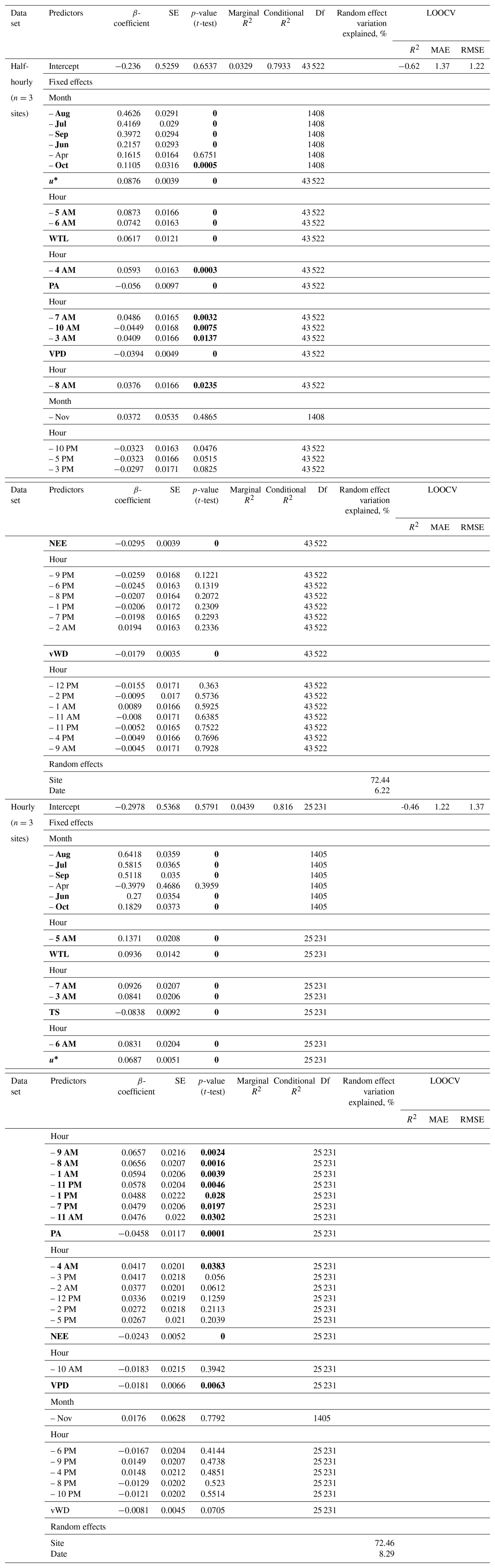
Table C15 Full linear mixed effects model results. In the models, absolute the difference between ecosystem- and plot-scale methane (CH₄) flux (FCH₄) (ΔFCH₄) was Yeo-Johnson-transformed, centered and scaled, while all continuous predictors were only centered and scaled. This table presents the full models with both nonsignificant and significant predictors before backward variable selection. The final daily and monthly models were the full models which are shown in Table 3 of the main text. Note that in all models temporal variables were included in nested random effects (see methods and Supplementary Methods A2). In all models, the reference level in site dominant vegetation (VEG) was Sphagnum moss, 0 in Hour and May in Month. Annual models were not included due to an inadequate number of observations. Due to lack of complete case observations, US-Owc was not included in the weekly and monthly models (n=7 sites). We excluded TS from the half-hourly model due to high multicollinearity with Month (VIF > 3). Due to multicollinearity in the weekly model, we built one model without NEE and one without VPD. Fixed effects are listed in decreasing order based on their β-coefficients. SE = standard error, Df = degrees of freedom of denominator, LOOCV = leave-one-out cross validation, MAE = mean absolute error, RMSE = root mean square error, PA = air pressure (kPa), u^* = friction velocity (m s⁻¹), WTL =  water table level (cm), TS = soil temperature (°C), NEE = net ecosystem exchange (µmol CO₂ m⁻² s⁻¹), VPD = vapor pressure deficit (hPa), vWD = v wind component (m s⁻¹), uWD = u wind component (m s⁻¹). Significant predictors are highlighted in bold.