Projected Effects of Climate-induced Changes in Phytoplankton biomass in the Southern South China Sea

Phytoplankton lies at the base of the marine pelagic food webs influencing the planet's net primary production and nutrient cycles. Understanding the impacts of anthropogenic climate change on the phytoplankton dynamics is crucial due to their pivotal role. Numerous studies across various latitudes have investigated the effects of climate change on the world's oceans, focusing on future projections on plankton. However, despite being one of the largest marginal seas of the world, the impact of such future projections on marine plankton in the South China Sea has rarely been documented. Monsoon derived productive upwelling areas in the South China Sea serve as ideal sites for studying plankton dynamics. In this study, a 3D coupled physical-biogeochemical model is used to examine the response of phytoplankton biomass and selected abiotic and biotic factors to future anthropogenic climate change, focusing on two upwelling areas of the southern South China Sea: Southeast Vietnam and Northwest Sabah. The results show declined phytoplankton biomass associated with warming and nutrient depletion, particularly silicate. However, the grazing pressure by mesozooplankton is predicted to be reduced, suggesting that this studied system is under bottom-up control. This study highlights the anticipated amplification of climate change-induced impacts on the phytoplankton over to higher trophic levels, which may influence both ecosystems and socioeconomics in the region.

1 Introduction

Phytoplankton plays a crucial role in Earth's ecosystems, representing only 1 % of planet's photosynthetic biomass, yet contributing to nearly half of the global net primary production (Field et al., 1998). Beyond their primary production role, phytoplankton contributes significantly to nutrient recycling while actively shaping marine food webs (Behrenfeld et al., 2006; Naselli-Flores and Padisák, 2023). Phytoplankton are microscopic organisms that are highly responsive to short and long-term environmental changes, exerting considerable influence on the dynamics of marine ecosystems. Their impact extends further into critical processes, including biogeochemical cycles and the structure of marine food webs (Yuan et al., 2018).

Since the onset of the industrial era, a substantial quantity of greenhouse gases has been discharged into the atmosphere due to human activities, causing noteworthy environmental changes (Pagès et al., 2020). According to the records, the average atmospheric carbon dioxide (CO₂) concentration, that remained around 280 ppm in the pre-industrial era, reached 419 ppm in 2023(Lindsey, 2024). About $\mathrm{1}/\mathrm{3}$ of these anthropogenically emitted atmospheric CO₂ is absorbed by the ocean, and therefore it plays a crucial role among the processes contributing to the removal of CO₂ from the atmosphere (Cao et al., 2009). However, as more CO₂ is being emitted, the increased ocean uptake leads to several adverse effects on the ocean, including warming, acidification, and deoxygenation (Bindoff et al., 2019). The significance of plankton and their vulnerability to the ongoing effects of climate change underlines the necessity of exploring the long-term patterns of plankton in the global oceans (Hays et al., 2005). Previous studies have shown projected declines in global phytoplankton biomass in a changing climate, with much-pronounced declines expected in tropical and subtropical regions (e.g., Bopp et al., 2013; Boyce et al., 2010; Henson et al.; 2021; Marinov et al., 2010). However, variations in regional climate patterns may introduce fluctuations around these projected trends (Boyce et al., 2010), highlighting the importance of carrying out climate studies on regional scales.

The South China Sea (SCS), which is among the world's largest marginal seas, has its unique variability due to the influence of both seasonal monsoons and the adjacent oceanic currents (Hou et al., 2022). In addition to its unique climatic features, the SCS retains its significance due to its vital role in fisheries, contributing to its socio-economic value (Pauly and Liang, 2020). Despite its importance, the studies on the impact of climate change on future plankton biomass in the SCS is less focused. Contrary to other marginal seas in the world such as the Mediterranean Sea (Pagès et al., 2020) and the Bering Sea (Chen et al., 2021; Hermann et al., 2013), studies have rarely used a modelling approach to form a future projection of the plankton dynamics in the SCS under climate change scenarios. Understanding these specific future impacts of climate change on the lower trophic levels helps to reflect its potential pressures on biodiversity as well as commercial fishing and socioeconomics in this region. This knowledge aids in developing mitigation strategies and the adaptation of appropriate policy frameworks.

This research primarily focuses on studying potential temporal and spatial shifts in the phytoplankton biomass, along with the key abiotic and biotic factors influencing these changes, in two selected upwelling areas of the Southern SCS driven by projected climate change impacts. Specifically, this study has focused on ocean warming from 1990 until year 2060, as outlined in the IPCC RCP8.5 (IPCC, 2014) emission scenario. In this study, the key external environmental factors chosen for analysis include temperature, nitrate and silicate as abiotic attributes (bottom-up drivers), and grazer/predator biomass as a biotic attribute (top-down driver) all of which are known to have major influence on phytoplankton biomass (Winder and Sommer, 2012). Since upwelling areas are extensively used as focal areas of phytoplankton research due to their role of bringing nutrient rich sub-surface waters to the sea surface and significantly enhancing phytoplankton blooms (Wu et al., 2019), the present study focuses on two key upwelling areas in the Southern SCS. These are, the Southeast Vietnam upwelling area and the Northwest Sabah upwelling area, both of which experience upwelling activity during monsoon seasons. Using model outputs from a specifically designed regional coupled 3-dimensional biophysical model, this research aims to assess temporal and spatial dynamics of the phytoplankton biomass and the selected abiotic and biotic environmental factors in the above upwelling areas during their respective monsoon seasons. Furthermore, the probable underlying relationships between the model-predicted spatio-temporal phytoplankton trends and external factors are discussed both in bottom-up and top-down regulatory contexts.

2 Materials and Methods

2.1 Study Area

The South China Sea (SCS) is a tropical, semi-enclosed shallow continental shelf in the Western Pacific Ocean, bordered by the land masses of East and West Malaysia, Vietnam, and Indonesia (Akhir, 2012). This region experiences distinct seasonal monsoons, where it is subjected to North-eastern monsoon (winter) and South-western monsoon (summer) from November to March and April to August, respectively. This area's bathymetry is characterized by shallow waters (< 100 m) over the shelf area which extends to deeper offshores (> 300 m) (Apriansyah et al., 2022). The surface circulation of SCS undergoes significant seasonal variations, influenced by these alternating monsoons, which could potentially change its biogeochemistry (Liu et al., 2002). These monsoonal winds induce coastal upwelling, giving rise to seasonally productive waters such as in the Southern Vietnam (Zhao et al., 2018), Eastern coast of peninsular Malaysia (Akhir et al., 2015) and Northwestern Sabah region on Borneo Island (Satar et al., 2020). However, this study focusses only on two upwelling regions: Southeastern Vietnam extending from 109–113° E and 9–13° N (Wu et al., 2019) and Northwestern Sabah extending from 114.5–118° E and 4.5–8° N (Satar et al., 2020) (Fig. 1). Upwelling occurs in the Southeast Vietnam region during the summer, while in Northwest Sabah, it takes place during the winter monsoon season. Moreover, to analyse the vertical profiles within these areas, coordinates were used based on previous studies in the Southeast Vietnam upwelling region (Xiao et al., 2020) and the Northwest Sabah upwelling region (Satar et al., 2020).

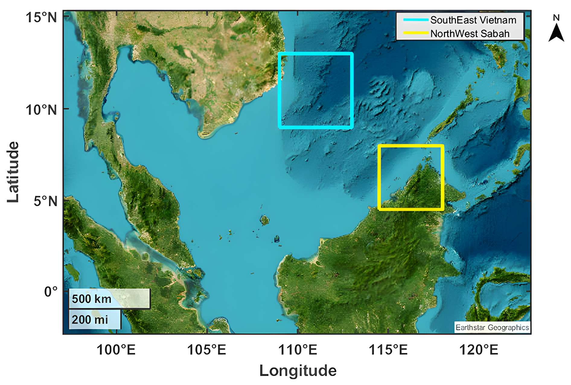
Figure 1 Map of the study area. The blue bounding box with coordinate ranges 109–113° E and 9–13° N shows the Southeast Vietnam upwelling region and yellow bounding box with coordinate ranges 114.5–118° E and 4.5–8° N shows the Northwest Sabah upwelling region.

2.2 The data sets

To study the dynamics of phytoplankton biomass in the SSCS upwelling regions in response to potential anthropogenic climate change, a pre-defined spatiotemporal subset from the validated simulation outputs of the SEAsia model (see Sect. 2.2.1 below) was used as the main input dataset. In addition, to evaluate the SEAsia model outputs for selected variables, both satellite-derived products and multi-observational datasets from Copernicus Marine Service corresponding to the selected years 2013, 2016, 2020, and 2023 were used as supporting observational datasets. These were: (i) Multi Observation Global Ocean 3D Temperature Salinity Height Geostrophic Current and MLD (https://doi/org/10.48670/moi-00052, CMEMS, 2026) and (ii) Global Ocean Colour (Copernicus-GlobColour), Bio-Geo-Chemical, L4 (monthly and interpolated) from Satellite Observations (1997–ongoing) (https://doi/org/10.48670/moi-00281, CMEMS, 2024).

2.2.1 Overview of the SEAsia model

The Southeast Asia (SEAsia: https://github.com/NOC-MSM/SEAsia, last access: 25 April 2026) model is a 3-dimensional (3D) regional configuration of the Nucleus for European Modelling of the Ocean (NEMO) coupled with a 1D biogeochemical model (see below). This coupled 3D model features a $\mathrm{1}/\mathrm{12}$° (9 km) resolution with 75 vertical levels incorporating hybrid-z coordinates and it uses the ORCA12 bathymetry (DRAKKAR Group, 2007).

The atmospheric conditions, including wind, short- and long-wave radiation, humidity, temperature, precipitation and pressure imposed on the model were derived from the HadGEM2 (CMIP5) Earth system model under the “historical climate” (1980–2004) and the “business as usual” IPCC RCP8.5 emission scenario (2005–2060). In addition, atmospheric CO₂ levels are imposed on the biogeochemical model (historical climate + RCP8.5). The model's lateral boundary conditions and initial conditions are derived from the global $\mathrm{1}/\mathrm{4}$° NEMO-MEDUSA ROAM simulation using identical surface forcing. The model incorporates 34 tidal constituents (FES2014 tide model), applied both as tidal potential and as sea surface height and barotropic currents along the open lateral boundaries of the model. The model also incorporates river runoff as part of its freshwater forcing, including major regional rivers.

The biogeochemical model coupled to the above SEAsia ocean circulation component is a comprehensive ecosystem model, named European Regional Seas Ecosystem Model (ERSEM: Butenschön et al., 2016). However, the ERSEM configuration coupled to the SEAsia model was slightly modified compared to the original ERSEM configuration, where Iron (Fe) cycle and Chlorophyll-a are not included in the SEAsia regional configuration. This model includes both pelagic and benthic ecosystem components whereas the present study focuses solely only on its pelagic part. The functional types of this ecosystem model are based on their ecosystem roles rather than specific species or taxa. The organisms in the ERSEM configuration are categorized into: (i) primary producers – i.e., picophytoplankton (< 2 µm), diatoms, nanophytoplankton (2–20 µm), and microphytoplankton (> 20 µm), (ii) primary consumers – i.e., mesozooplankton, microzooplankton, and nanoflagellates; (iii) and bacterial decomposers, along with (iv) particulate and dissolved organic matter (POM, DOM) in the pelagic zone. The state variables of this model include major chemical components for each functional type (carbon, nitrogen, phosphorus, silicate) where, a set of modules compute the rates of change of its state variables, considering the environmental conditions of the surrounding water body, physiological processes and predator-prey interactions (Butenschön et al., 2016; https://github.com/NOC-MSM/SEAsia, last access: 25 April 2026). This biogeochemical model employs fully dynamic stoichiometry for most of its functional types. The model dynamics of a living functional type are based on a standard organism influenced by the assimilation of carbon and nutrients into organic compounds through uptake. This also includes generic loss processes such as respiration, excretion, release, predation, and non-predatory (non-consumptive) mortality. A schematic diagram of the trophic interactions in the pelagic zone is shown in Fig. 2.

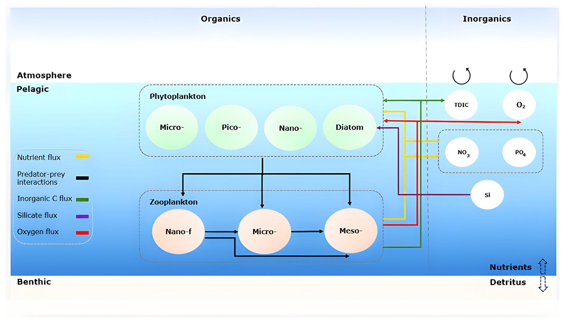
Figure 2 Schematic representation of the basic plankton interactions of the European Regional Seas Ecosystem Model (ERSEM).

2.2.2 Setting spatial, temporal and biological and environmental scopes

The spatial scope for the present study were the Southeast Vietnam and Northwest Sabah upwelling regions as described in Sect. 2.1 and Fig. 1 at approximately 9 km resolution. On the vertical dimension, the scope was narrowed down to the upper 120 m of the water column, where much of the primary production occurs in the photic zone of this region (Zhu et al., 2021). Furthermore, an examination of vertical profiles shows that the peaks of all variables occurred consistently within this depth range (see the Supplement). The temporal scope was a simulated timeseries extending from the year 1990 to 2060 (RCP8.5) at a monthly resolution. In terms of biology, the analyses focused mainly on the spatial and temporal dynamics of carbon biomass of phytoplankton. For the ease of analyses and interpretation, phytoplankton were divided into two classes: (i) diatom and (ii) non-diatom. The non-diatom biomass was considered as a unified (pooled) entity which is the sum of the carbon biomasses of picophytoplankton, nanophytoplankton and microphytoplankton. In this model, diatom group is characterized by their requirement of silicate, a characteristic not shared by other phytoplankton groups (Butenschön et al., 2016). For assessing the environmental dynamics, key variables (drivers) that are known to directly influence phytoplankton biomass were selected. These include seawater temperature and nutrient concentration – i.e., dissolved nitrate and silicate were selected as physicochemical (bottom-up) drivers. The grazer (mesozooplankton) biomass was selected as a biological driver that reflects the predation/grazing pressure on phytoplankton (top-down). The selected environmental variables, according to the model formulation and the previous studies, had the most significant forcing on phytoplankton entities of the SEAsia model (Butenschön et al., 2016; Winder and Sommer, 2012).

2.2.3 Comparing the model simulations and observations

As a first step, a comparison was conducted between observed (satellite-derived) and model-simulated mean sea surface temperature (SST) and phytoplankton carbon biomass during the upwelling monsoon seasons for four selected years (2013, 2016, 2020, and 2023) in the Southeast Vietnam and Northwest Sabah upwelling regions. These years were chosen to represent contrasting phases of interannual climate variability, including neutral, El Niño, and La Niña conditions, thereby enabling a robust assessment of model performance under different oceanographic regimes. This comparison had to be made focusing on the surface layer (> 0.5 m) because satellite-derived data were based on the sea surface. Further, despite satellite-derived primary production estimates were in Chlorophyll-a units (Chl.-a), the SEAsia biogeochemical model did not include Chl.-a component in its outputs. Therefore, the satellite-derived Chl.-a concentrations were converted to carbon units (biomass carbon) using region-specific Carbon : Chl.-a ratios, with values of 53.93 for Vietnam and 55.21 for Sabah. (Xu et al., 2021). It should be noted that satellite-derived ocean colour products are subject to well-documented limitations in coastal and upwelling environments, including reduced data availability and increased retrieval uncertainty associated with cloud cover, aerosol interference, and elevated concentrations of suspended particulate matter and coloured dissolved organic matter in nearshore waters (Xu et al., 2021). These factors may contribute to spatial and temporal gaps in the observational datasets used for model validation, particularly in the coastal sectors of both upwelling regions, and introduce an additional source of uncertainty in the model-observation comparison that is independent of model performance.

2.2.4 Exploring temporal and spatial dynamics

As the first step of assessing the spatio-temporal patterns in the data, latitude-, longitude-, time- and depth-specific physico-chemical (temperature, nutrients) and biological (diatom, non-diatom, mesozooplankton) data were extracted from the NetCDF4 files for the two upwelling regions separately. Here, the selected depth span (0–120 m) included 26 depth layers, where their arithmetic mean was obtained to reduce the spatial dimensionality of the data. Then, to further reduce temporal dimensionality of the data, these key variables were averaged over specific seasons, to allow for a more detailed analysis. In both upwelling regions, the productive season (= upwelling season) was focused on in the analyses. Here, in Southeast Vietnam upwelling area, the analysis focused on the Southwest or summer monsoon season (the average of months June, July and August) while in Northwest Sabah upwelling area, it is on the Northeast or winter monsoon season (the average of months December, January and February). When considering the temporal resolution, data on all the selected variables, except temperature, were calculated in monthly resolution. Due to this spatio-temporal dimensionality reduction, the Southeast Vietnam data included vertically averaged information for the summer monsoon season, while Northwest Sabah includes vertically averaged information for the winter monsoon season.

The dimensionality-reduced data were then used to study the: (i) temporal and (ii) spatial dynamics of phytoplankton (diatom and non-diatom) biomass, along with the selected key abiotic and biotic environmental variables that could potentially have driven these patterns. To study the temporal dynamics, timeseries analysis were performed on all variables across the two upwelling regions. For this, mean values for each variable were calculated separately for both the Southeast Vietnam and Northwest Sabah upwelling areas. Then, linear regression models were fitted to describe the overall trends or temporal patterns in the data. The adjusted R² values and the associated p-values of the fitted linear models were calculated on the observed trends of these timeseries to determine their significance. The observed trends were considered statistically significant at the 95 % confidence level (= 0.05 significance level). In addition, seasonal anomalies were calculated and plotted to examine the interannual variability of the selected variables (The formula is given below where, N=71 (1990–2060) and i= year).

$$\begin{array}{}\text{(1)}& \begin{array}{rl}\text{Seasonal anomaly}& ={\text{Seasonal mean}}_i\\ & -{\displaystyle \frac{\mathrm{1}}{N}}{\sum }_{j=\mathrm{1}}^N{\text{seasonal mean}}_j\end{array}\end{array}$$

Beside the observable temporal trends in the dataset, notable spatial variability existed (see Results). To study these spatial dynamics along the simulated timeseries, a two-step process was followed. Here, firstly, the timeseries was split into two sections, one focusing the proximal decade (1990–2000) and another focusing the distal decade (2050–2060) where the differential temporal change would be most pronounced under the simulated RCP8.5 based environmental forcing. Secondly, the percentage change of the phytoplankton (diatom and non-diatom) biomasses along with the other abiotic and biotic environmental variables across the two selected decades were calculated as:

$$\begin{array}{}\text{(2)}& \begin{array}{rl}\text{Percentage change}\left(\mathit{\%}\right)& ={\displaystyle \frac{({\mathrm{\mu }}_{\text{2050–2060}}-{\mathrm{\mu }}_{\text{1990–2000}})}{{\mathrm{\mu }}_{\text{1990–2000}}}}\\ & \times \mathrm{100}\end{array}\end{array}$$

To further understand the environmental drivers underpinning the above temporal and spatial patterns in the data a principal component analysis (PCA) was performed for the two upwelling regions separately.

2.3 Software and packages used

Data pre-processing was conducted using R studio version 2023.12.1 build 402 (RStudio Team, 2023) with the “ncdf4” package version 1.22 (Pierce, 2023). This step involved extracting specific coordinates of the selected domains, averaging the monthly values to obtain seasonal means, and averaging across depth layers. PCA plots were generated using the “ggplot2” package version 3.5.1 (Wickham, 2016). All the remaining statistical tests and figures including the map of the study area were generated using The MathWorks Inc. (2023) MATLAB (Version 2023b).

3 Results

3.1 Model Skill Assessment

A quantitative comparison between modelled and multi-observational SST across the four evaluation periods (2013, 2016, 2020, and 2023) is presented in Fig. 3. In the Southeast Vietnam upwelling region, the model demonstrates moderate to good agreement with observations, with R² values ranging from 0.65 in 2013 to 0.22 in 2023, and RMSE values remaining relatively low throughout (0.62–1.35 °C). A consistent negative bias was evident across all years (−0.29 to −1.29 °C), indicating a systematic cold bias in the modelled SST across the evaluation period. In Northwest Sabah, model skill was notably weaker in earlier years, with R² values of 0.05 and 0.00 recorded in 2013 and 2016 respectively, before improving substantially to 0.55 by 2023 (RMSE = 0.32 °C). Bias values in Sabah were small in magnitude but mixed in direction (−0.22 to +0.56 °C), suggesting no dominant systematic directional error in the thermal field, though the low R² values in earlier years indicate that the model fails to capture the spatial and temporal variance of observed SST in that region during those periods.

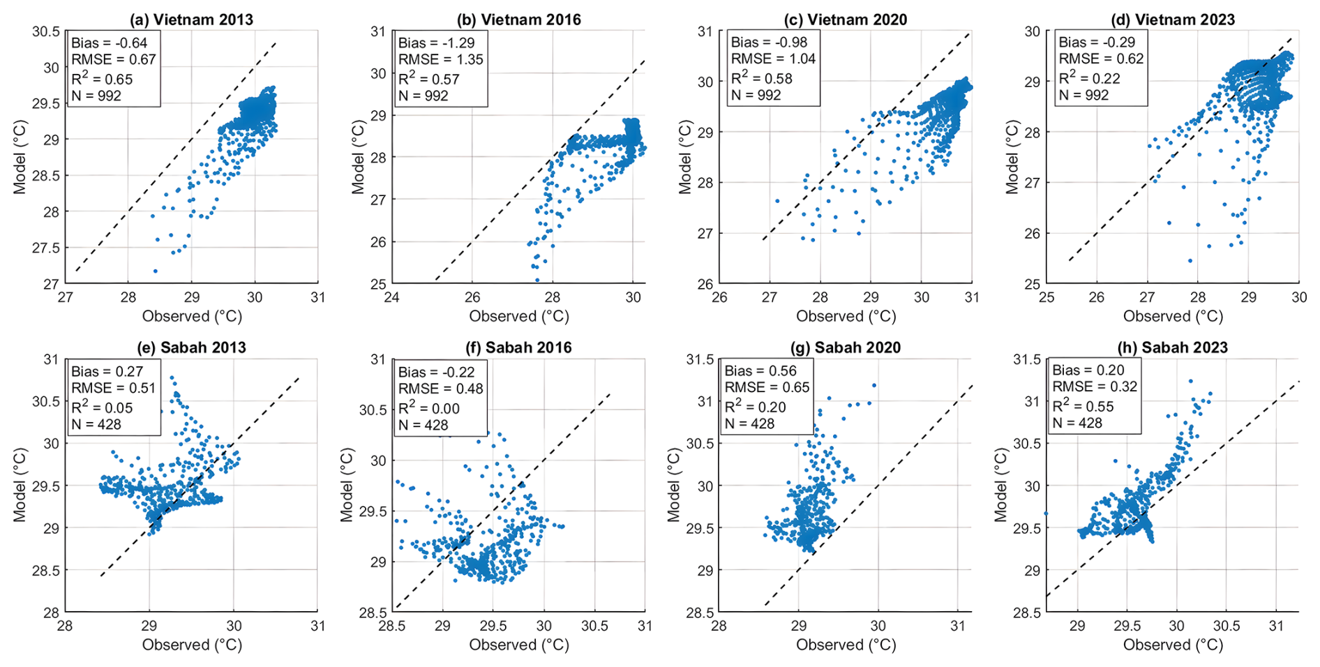
Figure 3 Scatter plots of modelled versus observed sea surface temperature (SST, °C) for the Southeast Vietnam (a–d) and Northwest Sabah (e–h) upwelling regions across four evaluation years: 2013 (a, e), 2016 (b, f), 2020 (c, g), and 2023 (d, h). The dashed line represents the 1:1 line of perfect agreement. Statistical metrics shown in each panel include bias (B, °C), root mean square error (RMSE, °C), coefficient of determination (R²), and number of data points (N). Observed SST data are derived from the Multi Observation Global Ocean 3D Temperature Salinity Height Geostrophic Current and MLD product (Copernicus Marine Service, https://doi/org/10.48670/moi-00052, CMEMS, 2026), which integrates satellite and in situ observations.

The model skill assessment for phytoplankton carbon biomass revealed greater variability and generally weaker performance compared to SST, reflecting the increased complexity of biological processes relative to physical state variables (Fig. 4). In Southeast Vietnam, R² values ranged from 0.28 to 0.80 across the evaluation years, with 2020 yielding the strongest agreement (R² = 0.80, RMSE = 8.47 mg C m⁻³) and 2023 the weakest (R²=0.28, RMSE = 12.32 mg C m⁻³). A positive bias was present across all Vietnam years, increasing progressively from 1.42 mg C m⁻³ in 2013 to 4.82 mg C m⁻³ in 2023, indicating a systematic and worsening tendency toward overestimation of carbon biomass. Inspection of the scatter plots reveals a characteristic fan-shaped distribution in Vietnam, wherein model-observation agreement is relatively close at low carbon biomass concentrations but diverges progressively at higher observed values, with the model underestimating bloom-level concentrations while overestimating at the low end of the distribution. In Northwest Sabah, model performance was substantially and persistently poorer, with R² values of 0.11 recorded consistently across 2013, 2016, and 2020, improving only marginally to 0.25 in 2023. Large negative biases ranging from −15.84 to −23.98 mg C m⁻³ and RMSE values between 53.16 and 70.53 mg C m⁻³ were recorded throughout, indicating that the model severely underestimates phytoplankton carbon biomass in this region. The scatter plots for Sabah show modelled values consistently compressed within a narrow range below 20 mg C m⁻³, irrespective of the magnitude of the observed concentrations, pointing to a fundamental inability of the model to reproduce the biological productivity characteristic of the Northwest Sabah coastal environment.

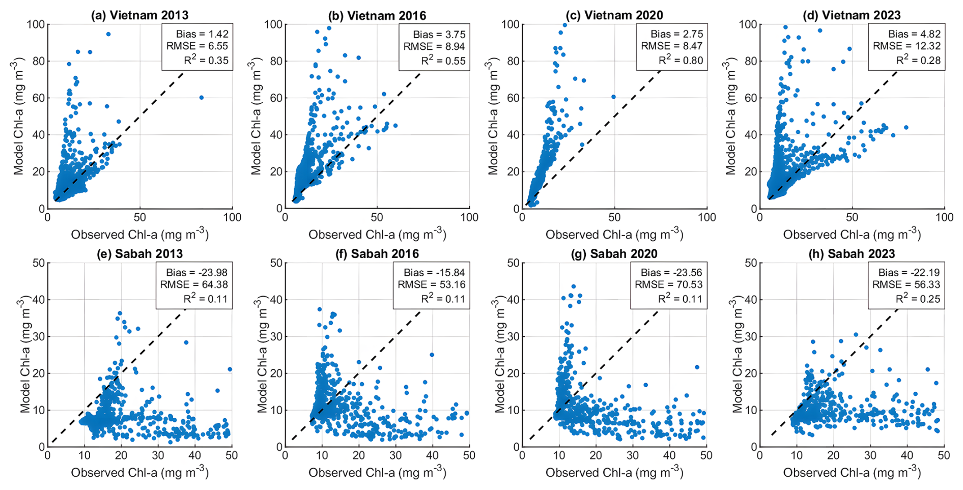
Figure 4 Scatter plots of modelled versus satellite-derived phytoplankton carbon biomass (mg C m⁻³) for the Southeast Vietnam (a–d) and Northwest Sabah (e–h) upwelling regions across four evaluation years: 2013 (a, e), 2016 (b, f), 2020 (c, g), and 2023 (d, h). The dashed line represents the 1:1 line of perfect agreement. Statistical metrics shown in each panel include bias (B, mg C m⁻³), root mean square error (RMSE, mg C m⁻³), and coefficient of determination (R²). Note that axes are scaled independently between the Vietnam and Sabah rows to aid visualisation. Satellite-derived phytoplankton carbon biomass was estimated from the Global Ocean Colour (Copernicus-GlobColour) L4 monthly product (https://doi/org/10.48670/moi-00281, CMEMS, 2024) using region-specific Carbon : Chl-a ratios of 53.93 for Vietnam and 55.21 for Sabah following Xu et al. (2021).

3.2 Temporal and spatial dynamics of the abiotic environment

3.2.1 Temperature

Temporal dynamics

The model-predicted mean seawater temperature of the upper 120 m in Southeast Vietnam exhibited a significant increasing trend over the 70-year period from 1990 to 2060, with an average increase of 0.02 °C per year (R²= 0.7573, p< 0.0001: Fig. 5a). Similarly, in Northwest Sabah (Fig. 5b), the temperature showed an average increase of 0.03 °C per year, which was also statistically significant (R²=0.7899, p< 0.0001: Fig. 5b). Atop these increasing trends, in both upwelling systems, seawater temperature varied notably interannually (Fig. 5a, b). These model-predicted increasing trends and the variability around it can also be seen in the anomaly plots (Fig. 5c, d). Here, the calculated seasonal anomalies: (i) became increasingly positive and (ii) more intense towards the end of the simulated timeseries (Fig. 5c, d). However, the magnitudes of the positive anomalies predicted for Southeast Vietnam (Fig. 5c) showed a greater variability among the adjacent years when compared to Northwest Sabah (Fig. 5d).

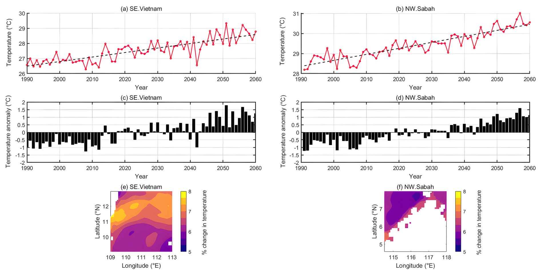
Figure 5 The seasonal mean temperature (a, b) of the upper 120 m of the water column during the upwelling seasons in Southeast Vietnam (a) and Northwest Sabah (b) predicted by the model for the 1990–2050 timeseries under the IPCC RCP8.5 scenario. Data are presented in °C. The black dotted line represents the trendline fitted to the data. The temperature (c, d) anomaly in Southeast Vietnam and Northwest Sabah upwelling areas. Percentage change in mean temperature (e, f) of the upper 120 m of the water column during the upwelling seasons in Southeast Vietnam (e) during summer and Northwest Sabah (f) during winter from 2050 to 2060 under the RCP8.5 scenario relative to the period 1990–2000.

Spatial dynamics

The notable interannual variations of mean seawater temperature of the upper 120 m in both upwelling systems appeared to have at least partly driven by its spatial heterogeneity (Fig. 5e, f). Comparing two decades in the proximal and distal ends of the timeseries, i.e., past (1990–2000) and future (2050–2060), the percentage change in the seasonal means of seawater temperature of the photic zone from 2050 to 2060 was on average 6.62 % higher (range = 5.56 %–8.05 %) compared to the period from 1990 to 2000 in the south Southeast Vietnam upwelling area (Fig. 5e). In Northwest Sabah upwelling area, the corresponding average temperature increase is 6.11 % with a range of 5.60 % and 6.78 % (Fig. 5f). According to the model-predicted spatial distribution pattern of seawater temperature over the upwelling regions, the areas typically characterized by cold upwelled waters have shown more intense temperature changes compared to adjacent open waters (Fig. 5e, f).

3.2.2 Nutrients

Temporal dynamics

The nitrate concentration in Southeast Vietnam exhibited no apparent trend over the simulated 70-year period from 1990 to 2060, with an average decrease of 0.001 mmol N m⁻³ yr⁻¹ (R²= 0.0039, p= 0.6030: Fig. 6a). Conversely, a statistically significant increasing trend was predicted for Sabah upwelling region, which encountered a 0.003 mmol N m⁻³ yr⁻¹ (R²= 0.1403, p= 0.0014: Fig.  6c) mean increase in the nitrate concentration over the simulated timeseries. Despite these model-predicted trends, in both upwelling regions, the model-simulated nitrate concentration shows a considerable interannual variability, which can also be observed in the anomaly plots (Fig. 6e, g).

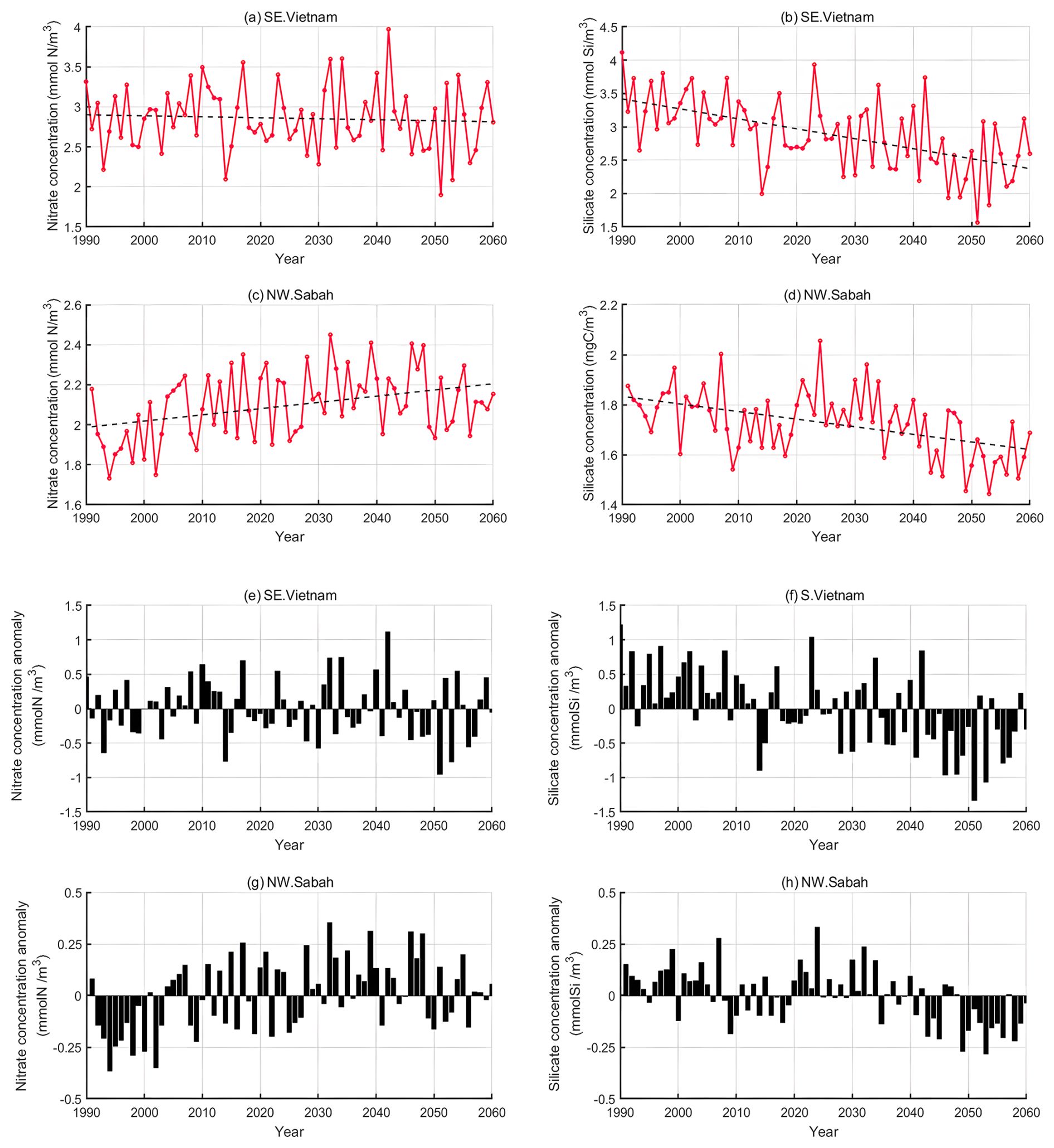
Figure 6 The seasonal mean Nitrate (a, c) and silicate (b, d) concentrations of the upper 120 m of the water column during the upwelling seasons in Southeast Vietnam (a, b) and Northwest Sabah (c, d) predicted by the model for the 1990–2050 timeseries under the IPCC RCP8.5 scenario. Data are presented in mmol m⁻³. The black dotted line represents the trendline fitted to the data. The nitrate (e, g) and silicate (f, h) concentration anomaly in Southeast Vietnam and Northwest Sabah upwelling areas.

The silicate concentration showed decreasing trends in both Southeast Vietnam (0.015 mmol Si m⁻³ yr⁻¹) and Northwest Sabah upwelling (0.003 mmol Si m⁻³ yr⁻¹) regions over the simulated 70-year timeseries from 1990 to 2060 (Fig. 6b, d). These model-predicted trends are statistically significant (Southeast Vietnam region: R²= 0.3162, p< 0.0001, Northwest Sabah region: R²=0.2310, p< 0.0001). Moreover, a higher interannual variability is observed in both areas over the period from 1990 to 2060. These model-predicted decreasing trends and the variability around it can also be seen in the anomaly plots (Fig. 6f, h). Here, the calculated seasonal anomalies: (i) became increasingly negative and (ii) more intense towards the end of the simulated timeseries (Fig. 6f, h).

Spatial dynamics

According to model simulations performed under RCP8.5 scenario, the model-predicted mean nitrate concentration in the southeast Vietnam upwelling area was 2.80 mmol N m⁻³ for 1990–2000 period and 2.76 mmol N m⁻³ for 2050–2060. As a percentage change, this is an average decline of 0.33 % across the two decadal periods (range = −12.77 %–60.22 %: Fig. 7a, b). The decline is more pronounced closer to the coast, while the greater range is due to some patches of very high variation (Fig. 7a). In Northwest Sabah upwelling area, the average increase of nitrate concentration from 1990–2000 to 2050–2060 periods was 14.45 % with a range from 0.30 % to 36.62 % (Fig. 7b). Here, the nitrate concentration in the upper 120 m increased from 1.91 mmol N m⁻³ to 2.09 mmol N m⁻³. However, the increase of mean nitrate concentration closer to the coast is more prominent when compared to the increase observed offshore (Fig. 7b).

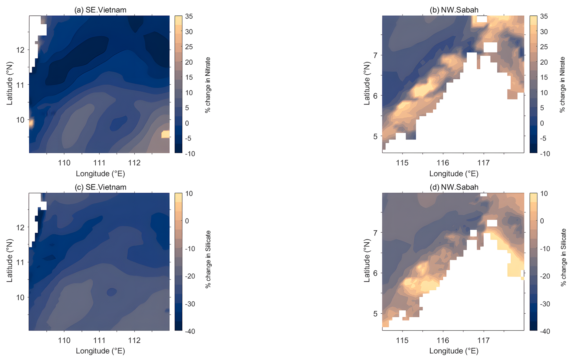
Figure 7 Percentage change in nitrate (a, b) and silicate (c, d) concentrations of the upper 120 m of the water column during the upwelling seasons in Southeast Vietnam (a, c) during summer and Northwest Sabah (b, d) during winter from 2050 to 2060 under the RCP8.5 scenario relative to the period 1990–2000.

The silicate concentration in the Southeast Vietnam upwelling area was 3.35 mmol Si m⁻³ for 1990–2000 period and 2.48 mmol Si m⁻³ for 2050–2060. As a percentage change, this is an average decline of 25.09 % across the two decadal periods (range = −46.59 %–−10.45 %: Fig. 7c). Here, the overall spatial variability is more similar to the pattern observed by the nitrate concentration in the same area. In Northwest Sabah upwelling area, the average decline from 1990–2000 to 2050–2060 periods was 9.53 % with a range from −44.98 % to 25.69 % (Fig. 7d). Here, the mean silicate concentration in the upper 120 m decreased from 1.79 mmol Si m⁻³ to 1.58 mmol Si m⁻³. The decline observed here is less than that in the Southeast Vietnam upwelling area with a comparatively broader range. Furthermore, in Northwest Sabah upwelling region, a decline in silicate concentration is observed towards offshore while it shows an increase near the coast (Fig. 7d). This observed spatial variation is similar to the pattern exhibited by nitrate concentration (Fig. 7b)

3.3 Temporal and spatial dynamics of the biotic environment

3.3.1 Temporal and spatial dynamics of the projected phytoplankton biomass

Temporal dynamics

The diatom biomass in Southeast Vietnam exhibited a significant declining trend over the simulated 70-year period from 1990 to 2060, with an average decrease of 0.027 mg C m⁻³ yr⁻¹ (R²= 0.0654, p= 0.0314). A similar statistically significant declining trend was predicted for Sabah upwelling region, which encountered a 0.026 mg C m⁻³ yr⁻¹ (R²= 0.0813, p= 0.0167) mean decrease in the diatom biomass over the simulated timeseries. Despite these trends, in both upwelling regions, the model-simulated diatom biomass varied considerably year-over-year (Fig. 8a, c). These model-predicted declining trends and the variability around it can also be seen in the anomaly plots (Fig. 8e, g). Here, the calculated seasonal anomalies: (i) became increasingly negative and (ii) more intense towards the end of the simulated timeseries (Fig. 8e, g). However, the magnitudes of the negative anomalies predicted for Northwest Sabah (Fig. 8g) were not as pronounced as in Southeast Vietnam (Fig. 8e).

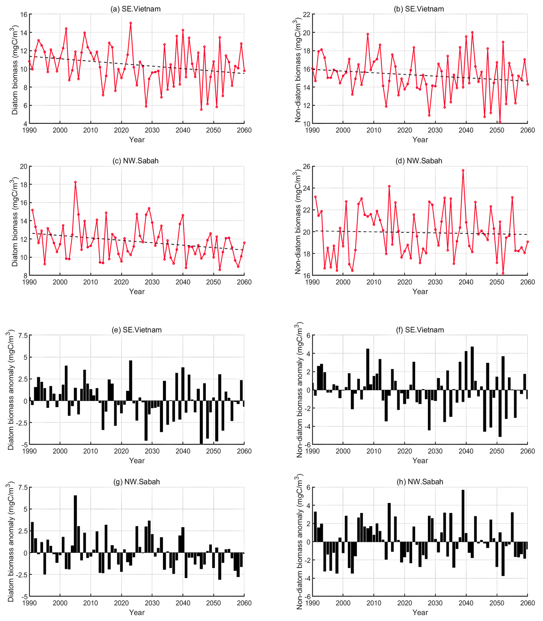
Figure 8 The seasonal mean diatom (a, c) and non-diatom (b, d) biomass of the upper 120 m of the water column during the upwelling seasons in Southeast Vietnam (a, b) and Northwest Sabah (c, d) predicted by the model for the 1990–2050 timeseries under the IPCC RCP8.5 scenario. Data are presented in mg C m⁻³. The black dotted line represents the trendline fitted to the data. The diatom (e, g) and non-diatom (f, h) biomass anomaly in Southeast Vietnam and Northwest Sabah upwelling areas.

The non-diatom biomass showed a slightly decreasing trend in Southeast Vietnam (slope $=-$0.018 mg C m⁻³ yr⁻¹, R²= 0.0304, p= 0.1456: Fig. 8b), though this trend did not reach statistical significance. In Northwest Sabah, no meaningful directional trend was evident in the non-diatom biomass over the simulated period (slope $=-$0.004 mg C m⁻³ yr⁻¹, R²= 0.002, p= 0.714: Fig. 8d), and the time series should be interpreted as exhibiting no net change over the 70-year simulation.

Spatial dynamics

According to model simulations performed under RCP8.5 scenario, the model-predicted mean diatom biomass in the south Vietnam upwelling area was 11.29 mg C m⁻³ for 1990–2000 period and 10.03 mg C m⁻³ for 2050–2060. As a percentage change, this is an average decline of 7.09 % across the two decadal periods (range $=-$29.81 %–15.41 %: Fig.  9a). The greater range around this decline signifies the notable spatial variability of diatom biomass (Fig. 9a), where the decline is more pronounced closer to the coast. In contrast, an increase in the diatom biomass of the upper 120 m was predicted by the model in some offshore areas (south and southeastern sectors) of Southeast Vietnam upwelling region (Fig. 9a). In Northwest Sabah upwelling area, the average decline from 1990–2000 to 2050–2060 periods was 11.92 % with a range from −30.50 % to 30.71 % (Fig. 9b). Here, the mean diatom biomass in the upper 120 m decreased from 12.14 mg C m⁻³ to 10.63 mg C m⁻³. However, decline of mean diatom biomass closer to the coast is less prominent when compared to the decline observed offshore (Fig. 9b).

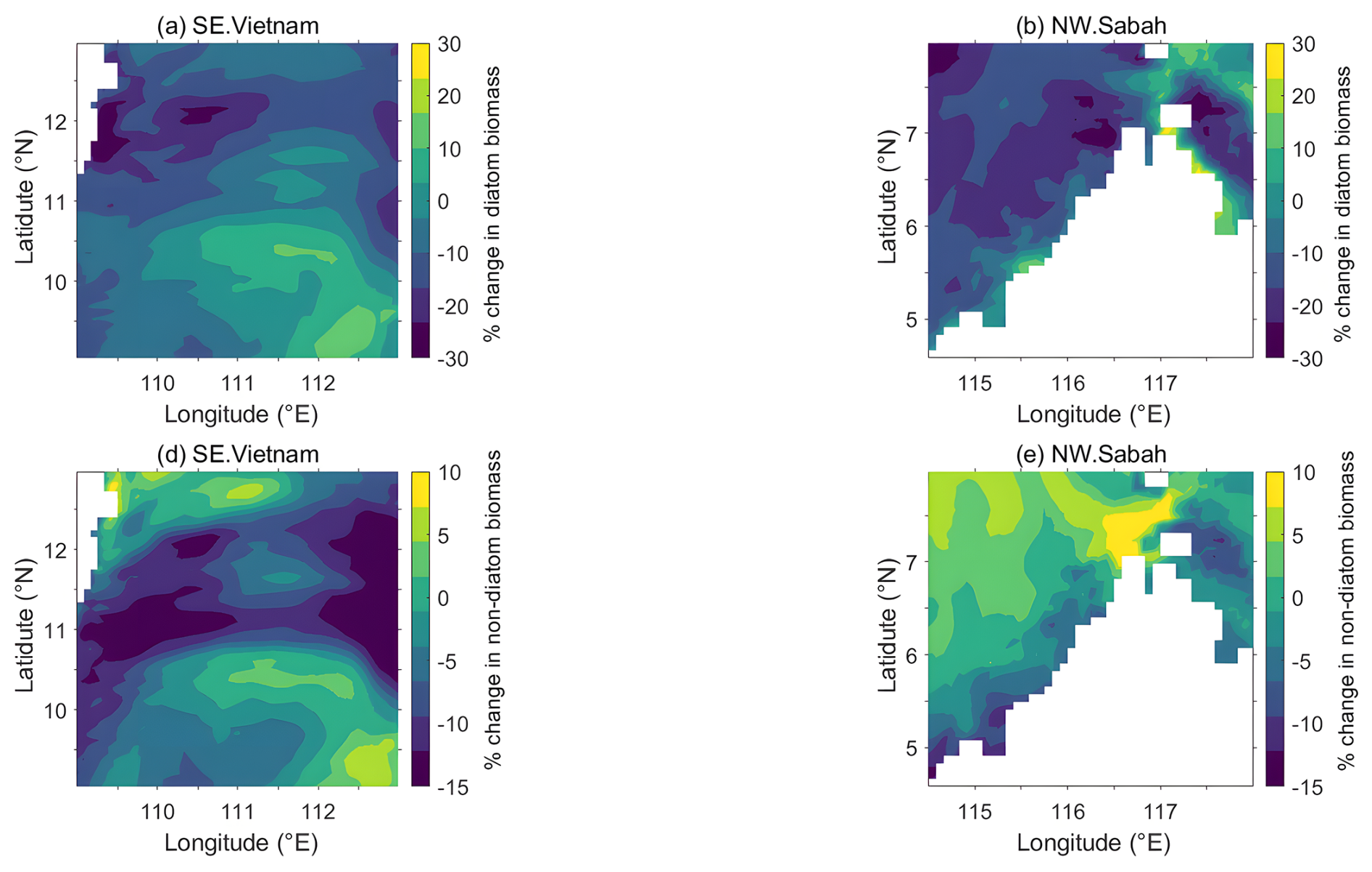
Figure 9 Percentage change in mean diatom (a, b) and non-diatom (c, d) biomass of the upper 120 m of the water column during the upwelling seasons in Southeast Vietnam (a, c) during summer and Northwest Sabah (b, d) during winter from 2050 to 2060 under the RCP8.5 scenario relative to the period 1990–2000.

The non-diatom biomass in the Southeast Vietnam upwelling area was 15.93 mg C m⁻³ for 1990–2000 period and 14.86 mg C m⁻³ for 2050–2060. As a percentage change, this is an average decline of 6.15 % across the two decadal periods (range $=-$21.05 %–8.71 %: Fig. 9c). Here, the overall spatial variability is more similar to the pattern observed by the diatom biomass in the same area. In Northwest Sabah upwelling area, the average decline from 1990–2000 to 2050–2060 periods was 0.25 % with a range from −16.34 % to 12.34 % (Fig. 9d). Here, the mean non-diatom biomass in the upper 120 m decreased from 19.26 mg C m⁻³ to 18.96 mg C m⁻³. The decline observed here is less than that in the Southeast Vietnam upwelling area and also has a comparatively narrower range. Furthermore, in Northwest Sabah upwelling region, a decline in non-diatom biomass is observed near the coast while it shows an increase towards offshore. This observed pattern contrasts with the pattern exhibited by diatom biomass (Fig. 9b, d). It should be noted that the substantial model-observation discrepancy in phytoplankton carbon biomass documented for Northwest Sabah (Fig. 4), where modelled values were persistently compressed within a narrow low-concentration range irrespective of observed magnitudes, introduces considerable uncertainty in the quantitative interpretation of the projected biomass changes for this region. Accordingly, the predicted magnitudes of phytoplankton biomass change in Northwest Sabah should be treated as indicative of directional trends rather than precise absolute values, and conclusions drawn from these projections should be interpreted with appropriate caution.

3.3.2 Temporal and spatial dynamics of the projected grazer biomass

Temporal dynamics

The model-predicted mesozooplankton biomass in the upper 120 m of the Southeast Vietnam upwelling region exhibited a significant declining trend over the 70-year period (1990–2060), with an average decrease of 0.019 mg C m⁻³ yr⁻¹ (R²= 0.0739, p= 0.0219: Fig.  10a). This trend is accompanied by very high interannual variability which is also noticeable in the anomaly plot (Fig. 10c). In Northwest Sabah (Fig. 10b), the mesozooplankton biomass showed an average decrease of 0.016 mg C m⁻³ yr⁻¹. However, unlike south Southeast Vietnam upwelling region, the decreasing trend in Sabah region was not statistically significant (R²= 0.0364, p-value: 0.1137). According to the calculated seasonal anomalies, mesozooplankton biomass become: (i) increasingly negative and (ii) more intense towards the end of the simulated timeseries (Fig. 10c, d).

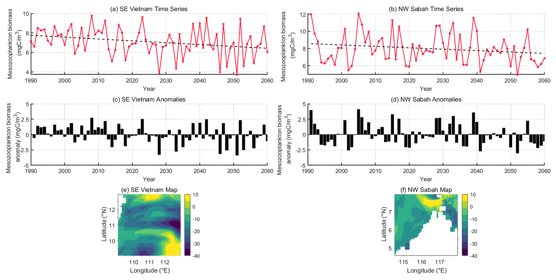
Figure 10 The seasonal mean mesozooplankton biomass (a, b) of the upper 120 m of the water column during the upwelling seasons in Southeast Vietnam (a) and Northwest Sabah (b) predicted by the model for the 1990–2050 timeseries under the IPCC RCP8.5 scenario. Data are presented in mg C m⁻³. The black dotted line represents the trendline fitted to the data. The mesozooplankton biomass (c, d) anomaly in Southeast Vietnam and Northwest Sabah upwelling areas. Percentage change in mean mesozooplankton biomass (e, f) of the upper 120 m of the water column during the upwelling seasons in Southeast Vietnam (e) during summer and Northwest Sabah (f) during winter from 2050 to 2060 under the RCP8.5 scenario relative to the period 1990–2000.

Spatial dynamics

Pronounced spatial heterogeneity of grazer distribution in the upper 120 m of the water column was a common characteristic of both upwelling regions (Fig. 10e, f). Consequently, the mean decline of grazer biomass along the timeseries was not spatially homogenous. Instead, according to the model predictions, despite percentage change in the seasonal mean mesozooplankton biomass in the distal decade of the timeseries (2050–2060) decreased by ca. 13.2 % compared to the proximal decade (1990–2000), it ranged between −41.59 % and 20.71 % (Fig. 10e) in the Southeast Vietnam upwelling region. The situation in Northwest Sabah upwelling area was not different from this where, the average decline of the mesozooplankton biomass in the upper 120 m was 10.65 % with a range from −44.98 % to 25.69 % (Fig. 10f). This massive range is due to the spatial heterogeneity of zooplankton distribution over the two upwelling regions, where the declining trends were some strong increases in some offshore areas in south Southeast Vietnam (Fig. 10e) and in northern coastal area of Sabah (Fig. 10f). Another observation is that the model-predicted spatial distribution pattern of mesozooplankton biomass in Southeast Vietnam region resembled that of both non-diatom and diatom biomasses of the same area (cf. Fig. 9a, c). In contrast, mesozooplankton biomass distribution in Northwest Sabah did not exhibit this resemblance.

3.4 Relationships between phytoplankton biomass and selected environmental factors

The general relationships between phytoplankton biomasses (diatom and non-diatom) and the environmental variables that have been discussed in the previous chapters are shown in Fig. 11a, b. The observed relationships between these variables differ across the two regions. In the PCA biplot for Southeast Vietnam, PC1 and PC2 collectively explain 88.94 % of the total variance in the data, whereas in Northwest Sabah, they explain 74.38 % of the variance. According to the Pearson's correlation performed, in Southeast Vietnam, diatom biomass has shown positive correlations with nitrate (r= 0.64, p< 0.0001), silicate (r= 0.72, p< 0.0001) and mesozooplankton (r= 0.94, p< 0.0001), while a negative correlation is observed with temperature (r= −0.62, p< 0.0001). For non-diatom biomass, positive correlations are observed with nitrate (r= 0.69, p< 0.0001) and mesozooplankton (r= 0.93, p< 0.0001) whereas a negative correlation is observed with temperature (r= −0.61, p< 0.0001).

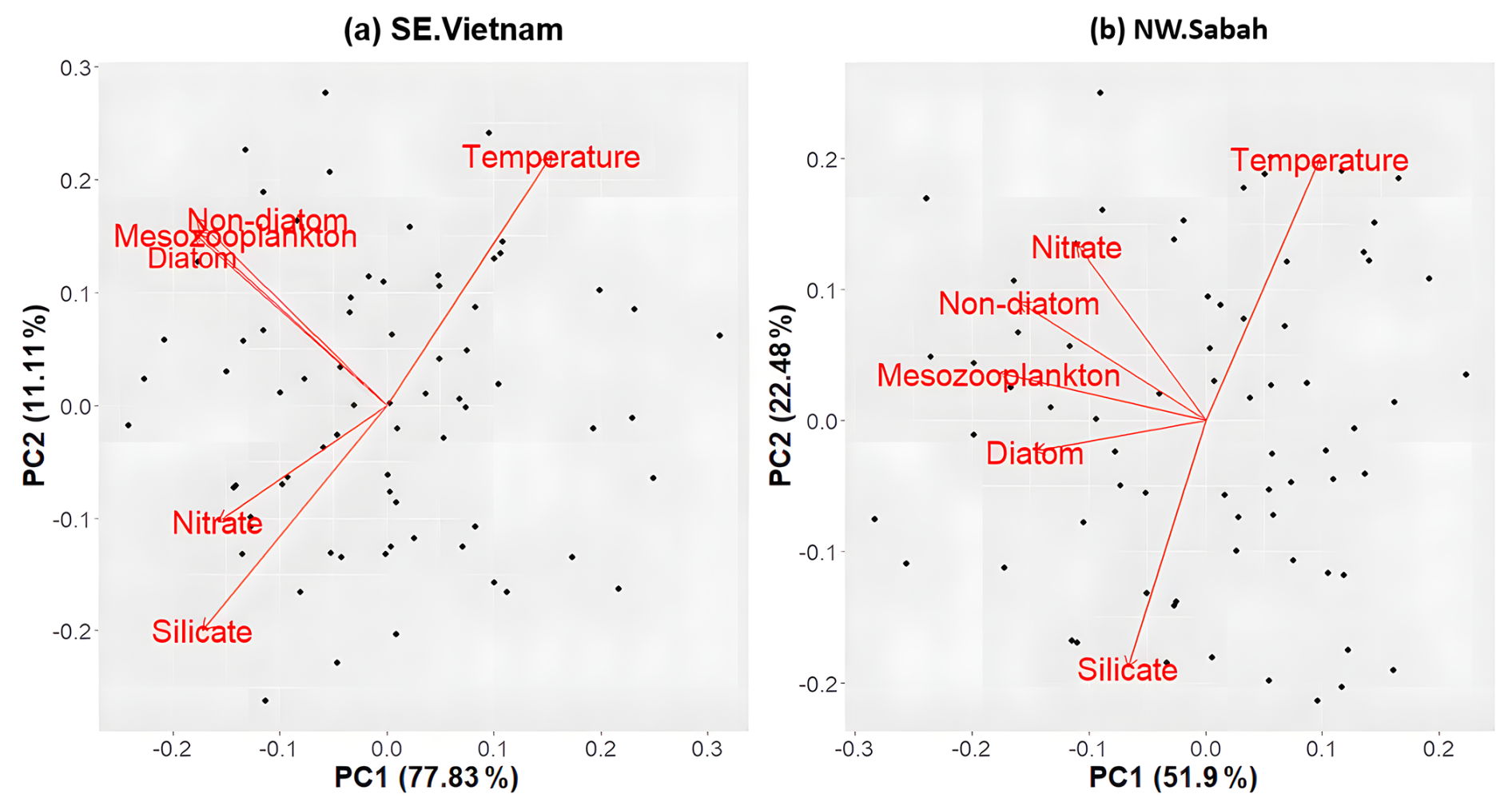
Figure 11 Principal Component Analysis (PCA) of seasonal means of phytoplankton biomass and the selected environmental variables in Southeast Vietnam (a) and Northwest Sabah (b) Regions (1990–2060). The arrows represent the variables, and the points represent the years. The arrows directed to same direction and are close to each other are positively correlated, arrows in opposite direction are negatively correlated and the arrows that are placed orthogonal have no relationship. It should be noted that vector orientation in PCA space reflects the contribution of each variable to the principal components, which capture directions of maximum shared variance across the full multivariate dataset. Apparent orthogonality between variables in the PCA biplot therefore reflects the absence of a shared variance structure along the principal component axes and does not necessarily contradict pairwise Pearson correlations computed independently between individual variables. Where discrepancies exist between PCA vector orientation and reported Pearson correlations, these should be interpreted with reference to the proportion of variance explained by each principal component and the potential influence of dominant variables on the ordination space.

In Northwest Sabah, diatom biomass has shown a positive correlation with mesozooplankton (r= 0.82, p< 0.0001). However, the correlations with nitrate (r= 0.21, p-value: 0.0798) and silicate (r= 0.19, p-value: 0.1037), were positive but not statistically significant. Similar to the findings in Southeast Vietnam, diatom biomass in Northwest Sabah has shown a negative correlation with temperature (r= -0.39, p-value: 0.0006). For non-diatom biomass, positive correlations are observed with nitrate (r= 0.62, p< 0.0001) and mesozooplankton (r= 0.87, p< 0.0001) whereas a negative correlation is observed with temperature (r= −0.32, p-value: 0.0062). It is noted that the PCA vector orientations for some variables, particularly in Northwest Sabah, may appear inconsistent with the pairwise Pearson correlations reported above. This reflects the difference between the two analytical approaches: Pearson correlations quantify the linear relationship between pairs of variables in isolation, whereas PCA vector orientation is determined by the contribution of each variable to axes of maximum multivariate variance, which can be dominated by variables with the largest absolute variance. These results should therefore be interpreted in conjunction with one another rather than in isolation.

4 Discussion

The present study focused on using output data from a coupled 3D biophysical model to analyze the response of phytoplankton biomass in two selected upwelling regions of the southern South China Sea, to anthropogenic climate change. The model predicts a notable decline in the upper-pelagial (≤ 120 m) diatom and non-diatom phytoplankton biomass over the analyzed 70-year timeseries (1990–2060: RCP8.5) (Fig. 8). These trends are accompanied by rising temperatures, declining silicate concentrations and fluctuating nitrate concentrations within the studied regions (Figs. 5, 6). Despite these temporal trends, a significant spatio-temporal heterogeneity was observed in the data, where the model-predicted phytoplankton biomass varied considerably: interannually and spatially across the study area. Statistical analyses revealed inverse relationship between temperature and silicate and a close association between diatom, non-diatom and mesozooplankton biomasses (Fig. 11). The declining phytoplankton biomass appeared to have negatively influenced the mesozooplankton grazers in the model, whose biomass also declined over time. This signifies how the impacts of anthropogenic climate change on the tropical ocean's biological productivity can transcend across trophic levels.

The decline of pelagic primary producer biomass predicted by the SEAsia model is somewhat consistent with the projections for the tropical western Pacific from previous global-scale studies on primary production (Bopp et al., 2013; Henson et al., 2021; Steinacher et al., 2010). However, since these studies have not specifically focused on the South China Sea, it is interesting to understand the drivers behind the observed decreasing trends in phytoplankton biomass within this region. According to global-scale studies, the projected reduction in primary production in tropics and mid-latitude regions, driven by climate change, is primarily caused by enhanced stratification, which results in decreased nutrient availability due to poor vertical mixing (Bopp et al., 2013; Chust et al., 2014; Dutkiewicz et al., 2013; Marinov et al., 2010).

The present study predicts rising temperatures, potentially intensifying stratification along the studied period until 2060 (Fig. 5a, b). This stratification is likely responsible for the model-predicted declining nutrient concentration trends, as evidenced by the declining silicate concentrations simulated in both upwelling regions (Fig. 6b, d). However, nitrate concentrations observed in both study areas did not follow this trend (Fig. 6a, c). These contrasting patterns could be due to differing regional oceanographic features. In the Southeastern Vietnam upwelling area, specifically the nitrate dynamics are influenced not only by upwelling but also by Mekong River runoff (Bombar et al., 2010). Similarly, in the Northwestern Sabah upwelling area, nutrient dynamics are affected by both upwelling and coastal river discharge (Baram river and Padas river), as well as surface water transport (Abbas et al., 2012), which may have contributed to these changes. Moreover, the model-predicted decline in silicate driven by warming-induced stratification may have contributed to the predicted reduction in diatom biomass. However, the predicted silicate decline appears to have had little influence on non-diatom biomass, as indicated by the absence of statistically significant declining trends in that group. In addition to the dependency on the discussed factors, biomass in the model relies on photosynthetically active radiation (PAR) (Butenschön et al., 2016). However, this is not analysed in the present study, as solar radiation is abundant in tropical regions, making nutrients a comparatively more significant limiting factor (Zhao et al., 2018). Although a direct diagnostic of stratification intensity such as pycnocline depth was not explicitly calculated from the model output in the present study, the co-occurrence of predicted surface warming and declining silicate concentrations is consistent with enhanced thermal stratification progressively reducing the upward flux of nutrient-rich subsurface waters into the photic zone. Quantification of pycnocline depth and its temporal evolution would strengthen this mechanistic interpretation and is recommended as a priority for future analyses of this dataset.

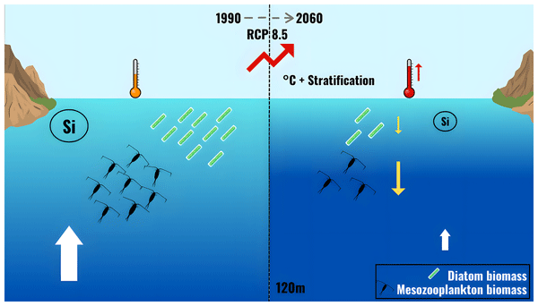
These results show that temperature and silicate imposed notable bottom-up control over the model-predicted phytoplankton biomass. Previous studies (e.g., Winder and Sommer, 2012) indicate that temperature significantly affects heterotrophic metabolism when compared to primary production. Warming is thus expected to boost grazing pressure, which imposes a stronger top-down control on phytoplankton. However, according to the present study, both phytoplankton (diatom and non-diatom) and grazer (mesozooplankton) biomasses have declined over the simulated timeseries (Figs. 8, 10a, b). For example, in Southeastern Vietnam upwelling region, the reduction of the diatom biomass from 1990 to 2060 was 7.09 % while mesozooplankton exhibited a biomass reduction of 13.20 %, which is nearly two-fold compared to phytoplankton. This indicates that rising temperatures, limited nutrients (silicate) and declining phytoplankton biomass had a negative impact on the mesozooplankton biomass (Fig. 11). This resembles the findings of Lewandowska et al. (2014) that in thermally-stratified, nutrient-limited waters, mesozooplankton (copepods) switch from feeding primarily on phytoplankton (diatoms) to smaller protists, such as ciliates – thus signifying the relative importance of the microbial loop. However, since diatoms have a much higher nutritional value compared to other protists such as ciliates (Lewandowska et al., 2014), this dietary shift may result in an overall decline in mesozooplankton biomass and condition. Despite the declining mesozooplankton biomass relaxed the grazing pressure on phytoplankton, the phytoplankton biomass simulated in the SEAsia model did not increase consequently (Figs. 8, 10a, b). This indicates that bottom-up forcing – i.e., temperature and nutrients had a much greater influence on the phytoplankton biomass than the grazing pressure on the top-down. Figure 12 summarizes these key results discussed above. However, some caution is necessary when interpreting these results, as biases may emerge from spatially averaging each variable across the selected domains. Nevertheless, a significant interannual variability remains even after spatial averaging, highlighting the inherent fluctuations within each region.

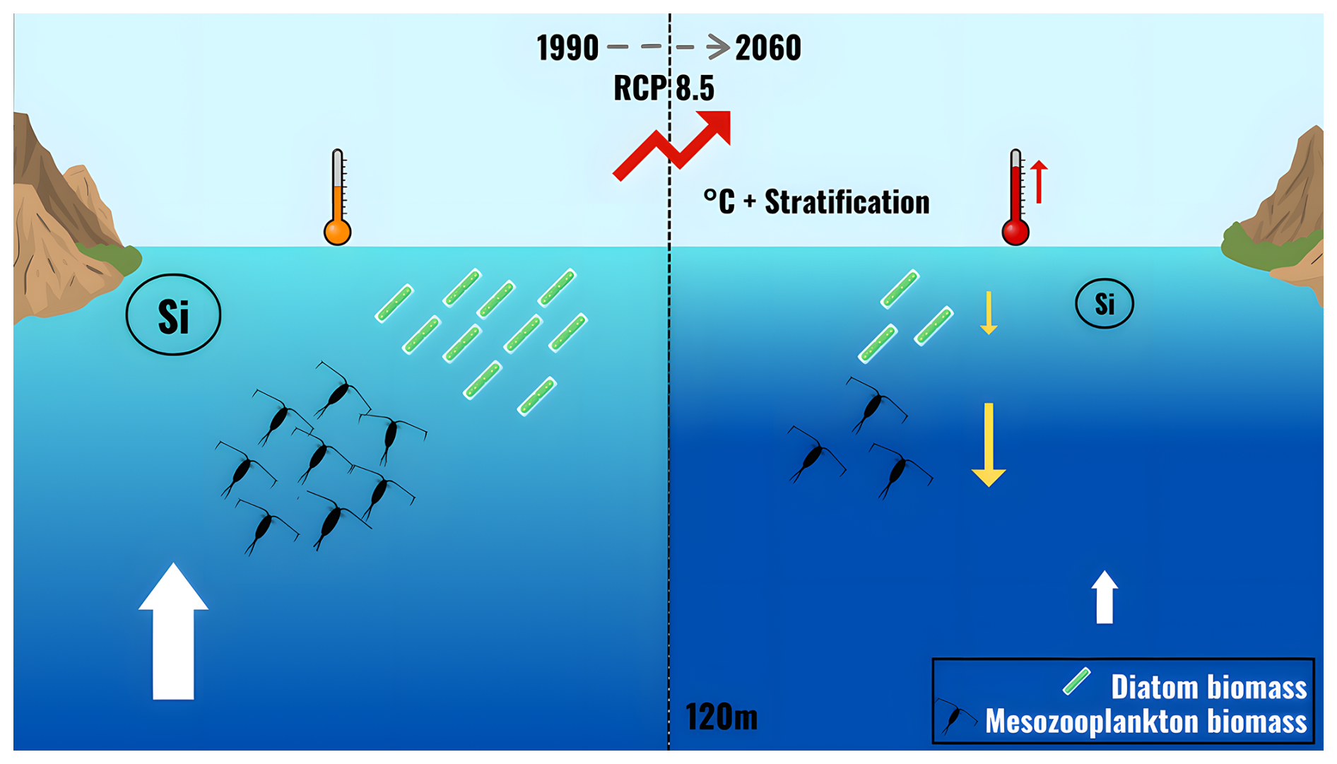
Figure 12 Schematic diagram summarizing the key results, illustrating an increasing trend in temperature according to the IPCC RCP8.5 climate scenario, likely increasing stratification of water column projected from 1990 to 2060. The diagram indicates how enhanced stratification has reduced upwelled nutrients (particularly silicate as observed in this study), resulting in a reduction in diatom biomass. This reduction is reflected in mesozooplankton biomass but in a greater magnitude, highlighting the transfer of climate change impacts across trophic levels. The width of the arrows in the diagram represents the magnitude of these changes, with upward arrows indicating increasing trends and downward arrows indicating decreasing trends.

In this study, the grazing pressure was characterized by the zooplankton biomass in the upper pelagial. There are two limitations of this approach. Firstly, the present analyses do not consider the vertical overlap between phyto- and zooplankton but focus on depth-averaged estimates for simplicity. Vertical positioning of predator and prey is an important metric that needs to be characterized in the future when further analyzing this dataset to render more accurate understanding of the grazing pressure (Cáceres et al., 2013; Greer et al., 2013). This is of particular significance given that both zooplankton and motile phytoplankton can perform tens-to-hundreds of meters deep diel vertical migrations (Brierley, 2014), which is not a part of SEAsia simulations. Secondly, this model accounts for neither plasticity nor evolution of body size among plankton. Recent individual based models have shown that especially, mesozooplankton body size is highly plastic to environmental variables, such as seawater temperature and phytoplankton concentration (Evans et al., 2020; Maps et al., 2012). Body size is a master life-history trait that can alter grazing, growth, developmental, metabolic and reproductive rates through allometric relationships (Carey and Sigwart, 2014). Further, models have shown that climate change driven shifts in thermal and feeding regimes in the ocean can lead to decrease in the average body size of mesozooplankton grazers (herbivorous copepods) and make them more numerous (Hays et al., 2005; Richardson, 2008). However, the SEAsia model does not consider the manifestations of zooplankton body size plasticity/evolution on phytoplankton biomass dynamics. Therefore, the present analyses may not render a full picture of the top-down selection pressure on phytoplankton dynamics.

Despite inherent limitations in the representation of biogeochemical processes at regional scales, several key physical and biological variables demonstrated sufficient agreement with observational data to justify the use of the ERSEM-SEAsia coupled model framework for the analysis of long-term phytoplankton carbon biomass dynamics and its covariability with temperature and nutrient forcing through 2060. The model-predicted SST showed moderate to good agreement with multi-observational data across both upwelling regions (Fig. 3), with R² values reaching 0.65 in Southeast Vietnam and 0.55 in Northwest Sabah, and RMSE values remaining below 1.35 °C throughout the evaluation period. The consistent negative bias in Vietnam SST (−0.29 to −1.29 °C), while systematic, is small in absolute magnitude and is likely associated with the use of IPCC RCP8.5 scenario forcing, which may introduce offsets in the thermal boundary conditions relative to the observational period, as previously noted for this model configuration. The improving SST skill in Northwest Sabah toward 2023 (R²= 0.55, RMSE = 0.32 °C) further supports confidence in the physical framework underpinning the projections, and the mixed bias direction in that region suggests no dominant systematic error in the representation of the thermal field.

The assessment of phytoplankton carbon biomass (Fig. 4) reveals greater uncertainty, particularly in Northwest Sabah, and these limitations must be considered in the context of the projection analysis. In Southeast Vietnam, the model demonstrated meaningful skill across most evaluation years, most notably in 2020 (R²= 0.80, RMSE = 8.47 mg C m⁻³), and the systematic positive bias, increasing from 1.42 mg C m⁻³ in 2013 to 4.82 mg C m⁻³ in 2023, is consistent in direction and predictable in magnitude, which is an important distinction from random error. As noted previously, a significant source of this discrepancy is likely attributable to the nature of the satellite-derived observational product itself: the carbon biomass estimates used for validation are derived from satellite Chl-a observations, an entity that is absent from the ERSEM configuration coupled to the SEAsia model. This fundamental difference in the quantities being compared introduces an irreducible source of uncertainty in the validation that is independent of model fidelity, and which likely contributes to both the magnitude and the variability of the bias across years and regions. Systematic biases of this nature, particularly where their origin is well understood, do not preclude the identification of long-term trends or the analysis of covariance between carbon biomass and physical and biogeochemical drivers, provided that conclusions are drawn from relative changes and directional trends rather than absolute modelled concentrations, an approach well established in the ocean biogeochemical modelling literature (Kwiatkowski et al., 2020).

In Northwest Sabah, the persistently low R² values (0.11 across 2013, 2016, and 2020) and large negative biases (−15.84 to −23.98 mg C m⁻³) represent a more substantive limitation. The modelled carbon biomass values remain compressed within a narrow low-concentration range irrespective of observed magnitudes, suggesting that the model underrepresents the high biological productivity characteristic of this coastal environment. This is consistent with the complexity of the Northwest Sabah coastal system, which is influenced by high terrigenous inputs, shallow bathymetry, and strong benthic-pelagic coupling in the southwestern Sulu Sea processes that are not fully resolved at the spatial scale of the current model configuration. However, the comparatively reasonable SST skill in Sabah confirms that the physical drivers underpinning the carbon biomass projections, including thermal stratification, upwelling intensity, and monsoon-driven circulation, are represented with sufficient fidelity to support physically consistent long-term projections. Furthermore, as with Vietnam, the additional uncertainty introduced by the Chl-a to carbon biomass conversion in the satellite-derived validation product likely contributes to the apparent magnitude of the model-observation discrepancy in Sabah, and the true model error in representing carbon biomass dynamics may be somewhat smaller than the raw statistics suggest. Projection results for Northwest Sabah should nonetheless be interpreted with appropriate caution, with quantitative conclusions regarding future carbon biomass magnitudes treated as indicative of directional change rather than precise absolute values.

Taken together, the model skill assessment supports the use of the ERSEM-SEAsia framework for the intended projection analysis, while underscoring the importance of interpreting outputs in terms of relative change, trend direction, and physical-biological covariance rather than absolute concentration magnitudes, particularly in the biogeochemically complex nearshore environment of Northwest Sabah. An overarching prediction of the present study is the negative (bottom-up) impact of the declining phytoplankton biomass on the adjacent trophic level (mesozooplankton grazers) in the studied upwelling areas of the southern South China Sea. It is understood that temperature-driven climate change impacts can intensify along marine food chains, because higher trophic levels are more sensitive to thermal stress and food depletion (Hu et al., 2022). In this specific case, it is worthy of investigating how far up the trophic chain that the impact of food depletion (= decrease of phyto- and mesozooplankton biomass) would reverberate within these two highly productive upwelling regions of the SSCS. It should be noted that while the SEAsia model projects declining phytoplankton and mesozooplankton biomass, the model does not extend to higher trophic levels such as fish, and the following discussion of potential fisheries impacts therefore represents a broader ecological inference rather than a direct model prediction.

In the SSCS, higher up in the food chain are various mesopelagic and epipelagic fish that for at least some part of their life cycle feed on zooplankton (e.g., herring, anchovies, younger stages of mackerel). These fish are commercially harvested and fish landings of the South China Sea accounts for staggering 12 % of the world's capture fisheries (11–17 ×10⁶ t by 2000s: Pauly and Liang, 2020; Teh et al., 2017). However, fish catches of this region have been declining lately due to overfishing and habitat destruction (Pitcher et al., 2000). Unfortunately, the current fisheries projections and management efforts in the (S)SCS do not consider the potential climate change impacts unraveled by the present study. Recent examples from some North Sea fish stocks (Dickey-Collas et al., 2010) show that when climate change impacts interact with other anthropogenic factors (e.g., overfishing) it can cumulate into catastrophic ecological and socioeconomic consequences. The SSCS pelagic ecosystem is already in an alarming state and how climate change driven decline of planktonic biomass would amplify this crisis should thus be investigated in detail before it is too late. The present study is, therefore, a small yet significant step in the correct direction, that needs to be expanded in the future.

5 Conclusions

This study provides insights on the potential effects of anthropogenic climate change on phytoplankton biomass, particularly diatom, in the Southern South China Sea by mid-century. Model predictions based on the SEAsia coupled 3D biophysical model outputs under the RCP 8.5 climate scenario have shown that the phytoplankton biomass (diatom and non-diatom) will decline from 1990 to 2060. This decline is accompanied by rising temperature trends likely leading to reduced nutrient concentrations, particularly silicate, possibly due to the warming-induced stratification that reduces upwelling. In addition to the declining phytoplankton biomass trends, the model predictions also indicate a declining trend in grazer biomass (mesozooplankton). Despite this release of the predation pressure on phytoplankton, which could have favoured an increase in the phytoplankton biomass, the decline has persisted, highlighting the influence of the bottom-up control within this ecosystem. Furthermore, the decline in mesozooplankton biomass is nearly two-fold in comparison to diatom biomass decline, which underlines the amplification of climate change induced impacts across trophic levels. To conclude this work, we recommend further research on the phytoplankton dynamics in relation to climate change in this region to better understand of its impacts and to determine to which extent these climate change impacts cascade across the trophic levels.