Solving calibration and reanalysis challenges of ocean biogeochemical dynamics with neural schemes: a 1D vertical model case-study

Numerous studies in climate and ocean sciences have highlighted the crucial role of ocean biogeochemical (BGC) models in studying and monitoring the global carbon cycle. Despite major advances due to both modelling and observation efforts, the quantification and reduction of the uncertainties in ocean BGC processes remain a key challenge. These difficulties arise primarily from the scarcity of observational datasets and the considerable uncertainties in ocean physics. Current ocean physics reanalyses still struggle to accurately represent the ocean's complex dynamics, particularly at small scales, which play a critical role in driving biogeochemical cycles. Consequently, the performance of operational ocean Data Assimilation (DA) systems remains limited when applied to BGC dynamics, using both BGC observations and physical reanalyses. This stands for model calibration and reanalysis applications.

Here, we explore machine learning approaches to address these challenges. To this end, we develop an Observing System Simulation Experiment (OSSE) framework for 1D ocean BGC dynamics, designed for both training and benchmarking purposes. We rely on a differentiable programming code of a 1D Nitrate-Ammonium-Phytoplankton-Zooplankton-Detritus (NNPZD) ocean BGC model forced by solar irradiance and vertical mixing. The proposed OSSE incorporates location-dependent uncertainties in physical forcings and considers realistic configurations of in situ observing systems. Based on these OSSEs, we design numerical experiments addressing both the calibration of BGC model parameters, the reconstruction of 1D ocean BGC state variables from sparse observations and the reduction of the uncertainties in the physical forcings. For calibration and inversion, we investigate a model-based variational DA scheme, an end-to-end deep learning scheme and their hybrid combination. Our results demonstrate the potential of learning-based schemes to substantially reduce calibration uncertainties and improve physical forcing estimates. When coupled with a variational DA scheme, the learning-based approach yields enhanced reconstructions of ocean BGC state variables. Sensitivity analyses with respect to forcing uncertainties and observing system configurations provide insights into how these findings could be extended to real-world ocean BGC modelling and monitoring.

1 Introduction

The global ocean plays a key role in the regulation of climate. Representing the largest carbon reservoir with 40 000 GtC (giga 10⁹ t of C) (Williams and Follows, 2011), it exchanges about 100 GtC and absorbs 2.8 GtC every year from the atmosphere (Friedlingstein et al., 2022). Because the global ocean limits the warming of the Earth, the need to understand and simulate its various processes has motivated the development of coupled physical–biogeochemical models. Physical models first enable us to quantify the physical (or solubility) pump: in high latitudes, atmospheric CO₂ gets easily dissolved into cold water and these shallow carbon-rich dense waters sink into the deep ocean exporting this dissolved inorganic carbon (DIC). The physical dynamics also play a key role in the biological pump, by driving the advection and diffusion of water masses and BGC tracers (Le Moigne, 2019; Boyd et al., 2019; Nowicki et al., 2022; Fossette et al., 2012; Lévy et al., 2013). Beyond this physics-driven processes, biogeochemical (BGC) models also represent processes of the biological pump that characterize the transformations of DIC into organic carbon (OC). From solar radiations, nutrients and inorganic carbon, phytoplankton performs photosynthesis into the photic layer (0–200 m), turning DIC into OC, which is the origin of the food chain. A fraction of this OC sinks, exporting carbon into deeper layers, while another fraction is fragmented and remineralized (i.e. turned into DIC) by zooplankton and bacterial activity (Lampitt et al., 1990). The export flux regulates carbon storage in the deep ocean for several years, or even several hundred years, and the energy input needed to supply the metabolic demand in the mesopelagic zone. Coupling physical and biogeochemical models enable us to quantify the overall contribution of the biological carbon pump, estimated at 6 to 13 GtC yr⁻¹ (Nowicki et al., 2022).

The evaluation and calibration of ocean BGC models remains a key challenge to reduce biases and uncertainties in the monitoring and simulation of the ocean cycle (Kaufman et al., 2018; Dowd et al., 2014; Kane et al., 2011). In this respect, ocean observing systems cannot cover the full range ocean processes and scales at play. Satellite sensors capture ocean dynamics on a synoptic scale (Groom et al., 2019; McClain, 2009). Nonetheless, this information only represents the surface state, presenting sampling gaps due to cloud coverage (Gregg et al., 2007). Similarly, for ocean physics, satellite-derived observations are also mainly limited to the surface and hardly resolve fine-scale dynamics for horizontal scales below one hundred kilometers (Ballarotta et al., 2019). Monitoring the interior of the oceans is even more complex. In situ networks such as ARGO floats, moored buoys, scientific cruises deploy numerous tools to sample specific BGC ocean parameters, such as plankton diversity, bacterial activity, particle distribution. However, this complementary information remains very scarce (Gould et al., 2013; Claustre et al., 2020) and gathers highly heterogeneous parameters (Claustre et al., 2020). From a methodological point of view, data assimilation schemes provide generic numerical approaches to address model calibration issues from multi-source observation datasets (Cossarini et al., 2019; Yao and Schlitzer, 2013). The uncertainties and biases in ocean physics reanalyses, especially regarding small-scale processes, however impede in general the direct exploitation of data assimilation schemes for the calibration of ocean BGC models (Pasquier et al., 2023; Bagniewski et al., 2011; Friedrichs et al., 2007). This consequently limits their application in the reconstruction and forecasting of BGC variables (Pasquier et al., 2023; Doney et al., 2004; Bagniewski et al., 2011; Friedrichs et al., 2007).

Deep learning has emerged over the last decade as a new class of data-driven schemes to address a variety of inverse problems in geoscience. We may cite among others short-term forecasting problems (Fablet et al., 2021a; Farchi et al., 2021b), reconstruction problems from partial observations (Zinchenko and Greenberg, 2024; Febvre et al., 2024; Ouala et al., 2018), model calibration and correction issues (Brajard et al., 2021; Buchanan et al., 2025; Couvreux et al., 2021; Gupta and Lermusiaux, 2023), downscaling and emulation problems (Gottwald and Reich, 2021; Farchi et al., 2021a; Brajard et al., 2021). Most deep learning schemes rely on supervised learning strategies meaning that a training phase optimizes the parameters of a neural scheme so that it will best map the considered inputs to the targeted outputs according to a predefined performance score (Naidu et al., 2023). In the context of oceanographic studies, the combination of deep learning strategies and OSSEs (Observing System Simulation Experiment) emerges as a relevant approach to design realistic training strategies. OSSE frameworks provide experimental testbeds to evaluate and characterize the impact of observing systems and the performance of data assimilation systems. Recent studies also demonstrate how to leverage OSSE-based datasets to train neural networks in a supervised manner for their application to real observation datasets (Littaye et al., 2025b; Archambault et al., 2024; Febvre et al., 2024).

Following our previous study with a simplified 0D BGC model (Littaye et al., 2025b), we aim to investigate further how deep learning schemes could enhance the development and calibration of ocean BGC models when dealing with forcing uncertainties and sparse observations. We develop a realistic 1D ocean BGC case-study based on a Nitrate-Ammonium-Phytoplankton-Zooplankton-Detritus (NNPZD) model in a spatio-temporal ocean environment (time and vertical dimension – 1D). The proposed experimental testbeds address both the calibration of the ocean BGC model parameters and the reanalyses of ocean BGC states given partial observations and noisy forcings. We evaluate a variational data assimilation method and a supervised learning-based framework. The latter exploits an OSSE-based training strategy to learn a mapping from noisy forcings and partial observations to model parameter and state estimates. In addition, we propose a novel hybrid method, that integrates the physical and BGC reanalysis of the learning-based model and a variational scheme to reduce the BGC reanalysis error. Our results support the potential of deep learning schemes to improve the calibration of ocean BGC models as well as to enhance the reanalysis of ocean BGC dynamics.

The structure of the paper is as follows. Section 2.2 introduces the considered case study, i.e., the BGC model, the physical forcings and how the forcing uncertainty is formulated. Section 3 presents the problem at stake, the two calibration methods and the metrics that are used to evaluate the calibration performance. Section 4 reports our numerical experiments and Sect. 5 discusses the main findings of our study and their relevance for future research.

2 Case-studies and Datasets

This section presents the data used in this study. Specifically, we detail the provenance of the data which is partly collected from existing databases, and describe the remaining data that has been precisely generated for this study. The section also delineates the various assumptions and methodologies to scale with data of varying quality levels, with the scenarios that were considered.

2.1 Considered physics-BGC model

The study relies on a differentiable 1D framework with a physical (Eq. 1) and a biological component (Eq. 2). The first right-hand term resolves the physics, that is the vertical diffusion of the tracer with a space-time-varying diffusion coefficient K_z. The second term SMS(C) accounts for the non conservative (Source Minus Sink: SMS) processes of tracer C, i.e. the BGC processes described in Eq. (2). A no-flow boundary condition, defined as ${\mathbf{K}}_z\frac{\partial \mathbf{C}}{\partial z}=\mathrm{0}$, is imposed for the diffusion at each boundary. This Neumann condition guarantees no vertical outflows between the surface and the atmosphere nor between the water column and the seafloor.

$$\begin{array}{}\text{(1)}& {\displaystyle \frac{\partial \mathbf{C}}{\partial t}}={\displaystyle \frac{\partial }{\partial z}}\left({\mathbf{K}}_z{\displaystyle \frac{\partial \mathbf{C}}{\partial z}}\right)+\mathrm{SMS}\left(\mathbf{C}\right)\end{array}$$

The NNPZD model (Eq. 2) is inspired by Newberger et al. (2003). This model describes nitrogen concentration dynamics across five compartments: nitrate (NO₃), ammonium (NH₄), phytoplankton (P), zooplankton (Z), and detritus (D). The equations are defined over time and space (vertical dimension). However, to avoid excessive notation, the space dimension is omitted. They involve 16 fixed BGC parameters and 2 time- and space-varying physical forcings and state the time dynamics of these compartments as Ordinary Differential Equations (ODEs):

$$\begin{array}{}\text{(2)}& \left\{\begin{array}{ll}\frac{{\mathrm{dNO}}_{\mathrm{3}}}{\mathrm{d}t}& =\mathit{\mu }{\mathrm{NH}}_{\mathrm{4}}-\mathbf{G}\frac{{\mathrm{NO}}_{\mathrm{3}}}{\mathit{\kappa }+{\mathrm{NO}}_{\mathrm{3}}}{e}^{-\mathrm{\Psi }{\mathrm{NH}}_{\mathrm{4}}}\mathrm{P}+\mathit{\lambda }\left(\mathit{\beta }-{\mathrm{NO}}_{\mathrm{3}}\right)\\ {\displaystyle \frac{{\mathrm{dNH}}_{\mathrm{4}}}{\mathrm{d}t}}& =-\mathbf{G}\frac{{\mathrm{NH}}_{\mathrm{4}}}{\mathit{\kappa }+{\mathrm{NH}}_{\mathrm{4}}}\mathrm{P}-\mathit{\mu }{\mathrm{NH}}_{\mathrm{4}}+\mathrm{\Gamma }\mathrm{Z}+\mathit{\phi }\mathrm{D}\\ {\displaystyle \frac{\mathrm{dP}}{\mathrm{d}t}}& =\mathbf{G}\left(\frac{{\mathrm{NO}}_{\mathrm{3}}}{\mathit{\kappa }+{\mathrm{NO}}_{\mathrm{3}}}{e}^{-\mathrm{\Psi }{\mathrm{NH}}_{\mathrm{4}}}+\frac{{\mathrm{NH}}_{\mathrm{4}}}{\mathit{\kappa }+{\mathrm{NH}}_{\mathrm{4}}}\right)\mathrm{P}-\mathrm{\Xi }\mathrm{P}\\ & -\mathit{\rho }\left(\mathrm{1}-e^{-\mathrm{\Lambda }\mathrm{P}}\right)\mathrm{Z}\\ \frac{\mathrm{dZ}}{\mathrm{d}t}& =(\mathrm{1}-\mathit{\gamma })\mathit{\rho }\left(\mathrm{1}-e^{-\mathrm{\Lambda }\mathrm{P}}\right)\mathrm{Z}-\mathrm{\Gamma }\mathrm{Z}\\ \frac{\mathrm{dD}}{\mathrm{d}t}& =\mathit{\gamma }\mathit{\rho }\left(\mathrm{1}-e^{-\mathrm{\Lambda }\mathrm{P}}\right)\mathrm{Z}+\mathrm{\Xi }\mathrm{P}-\mathit{\phi }\mathrm{D}+\frac{\partial {\mathbf{\Phi }}_{\mathrm{sed}}\left(\mathrm{D}\right)}{\partial z}\end{array}\right.\end{array}$$

The 16 parameters (listed in Table 1) represent physical and BGC sub-processes. The G factor symbolizes the photosynthesis process, denoted as $\mathbf{G}=\mathit{\eta }\frac{\mathit{\alpha }I(t,z)}{\sqrt{{\mathit{\eta }}^{\mathrm{2}}+{\mathit{\alpha }}^{\mathrm{2}}\mathbf{I}(t,z{)}^{\mathrm{2}}}}$, with $\mathbf{I}(t,z)={\mathit{I}}_{\mathrm{0}}\left(t\right)e^{\mathit{\xi }z+\mathit{\zeta }{\int }_{\mathrm{0}}^z\mathrm{P}(t,z^{\prime })\mathrm{d}{z}^{\prime }}$ the photosynthetically available radiation (PAR) at depth z and time t, the PAR at the surface being denoted by I₀. The total nitrogen uptake by phytoplankton is given by $\mathbf{G}\left(\frac{{\mathrm{NO}}_{\mathrm{3}}}{\mathit{\kappa }+{\mathrm{NO}}_{\mathrm{3}}}{e}^{-\mathrm{\Psi }{\mathrm{NH}}_{\mathrm{4}}}+\frac{{\mathrm{NH}}_{\mathrm{4}}}{\mathit{\kappa }+{\mathrm{NH}}_{\mathrm{4}}}\right)\mathrm{P}$. The zooplankton grazing upon phytoplankton is formulated by $\mathit{\rho }(\mathrm{1}-e^{-\mathrm{\Lambda }\mathrm{P}})\mathrm{Z}$, where a part of it goes to detritus through excretion and mortality with the term $\mathit{\gamma }\mathit{\rho }(\mathrm{1}-e^{-\mathrm{\Lambda }\mathrm{P}})\mathrm{Z}$. The terms μNH₄, ΓZ, φD and ΞP stands for ammonia oxidation, zooplankton respiration, remineralisation and phytoplankton death processes, respectively.

The detritus compartment is affected by gravity and sinks with a sinking rate ω. This process is represented by $\frac{\partial {\mathbf{\Phi }}_{\mathrm{sed}}\left(\mathrm{D}\right)}{\partial z}=\frac{\partial \mathit{\omega }\mathrm{D}}{\partial z}$ for detritus, with a sedimentation flux Φ_sed defined through a third-order WENO scheme (Liu et al., 1994). This flux is equal to zero at the surface, given the absence of fluxes at the air-sea interface. In the absence of advection and horizontal diffusion, the sinking of detritus leads to the depletion of nitrogen from the system over time. Indeed, the sinking nitrogen remains too deep to be mixed to the surface during winter. In order to compensate for this loss, which is not compensated for by 1D dynamics, an additional term is introduced in order to replenish the nutrient profile and ensure a steady state (Fennel et al., 2003). This so-called nudging (Ortega et al., 2017), is formulated as λ(β−NO₃). We assume that this nitrate supply occurs during the month of February, when the Mixed Layer is the deepest. We set the parameter λ to 0.05 d⁻¹ during February and to 0 d⁻¹ otherwise. As the depth of the mixed layer is among the key driver of nutrient fluxes from the deep ocean to the upper ocean (Williams et al., 2006), we parameterize reference concentration β with respect to the seasonally maximum of the mixed layer depth (MLD) and the NO₃ profile (Appendix A).

Table 1 Table of the BGC parameters (first and second lists), the physical forcings (third list), their definition, reference value and unit. The first list gathers the BGC parameter to constrain and the second lists the BGC parameters that are fixed. The choice of which parameter to constrain is supported by an initial sensitivity analysis (see Appendix B).

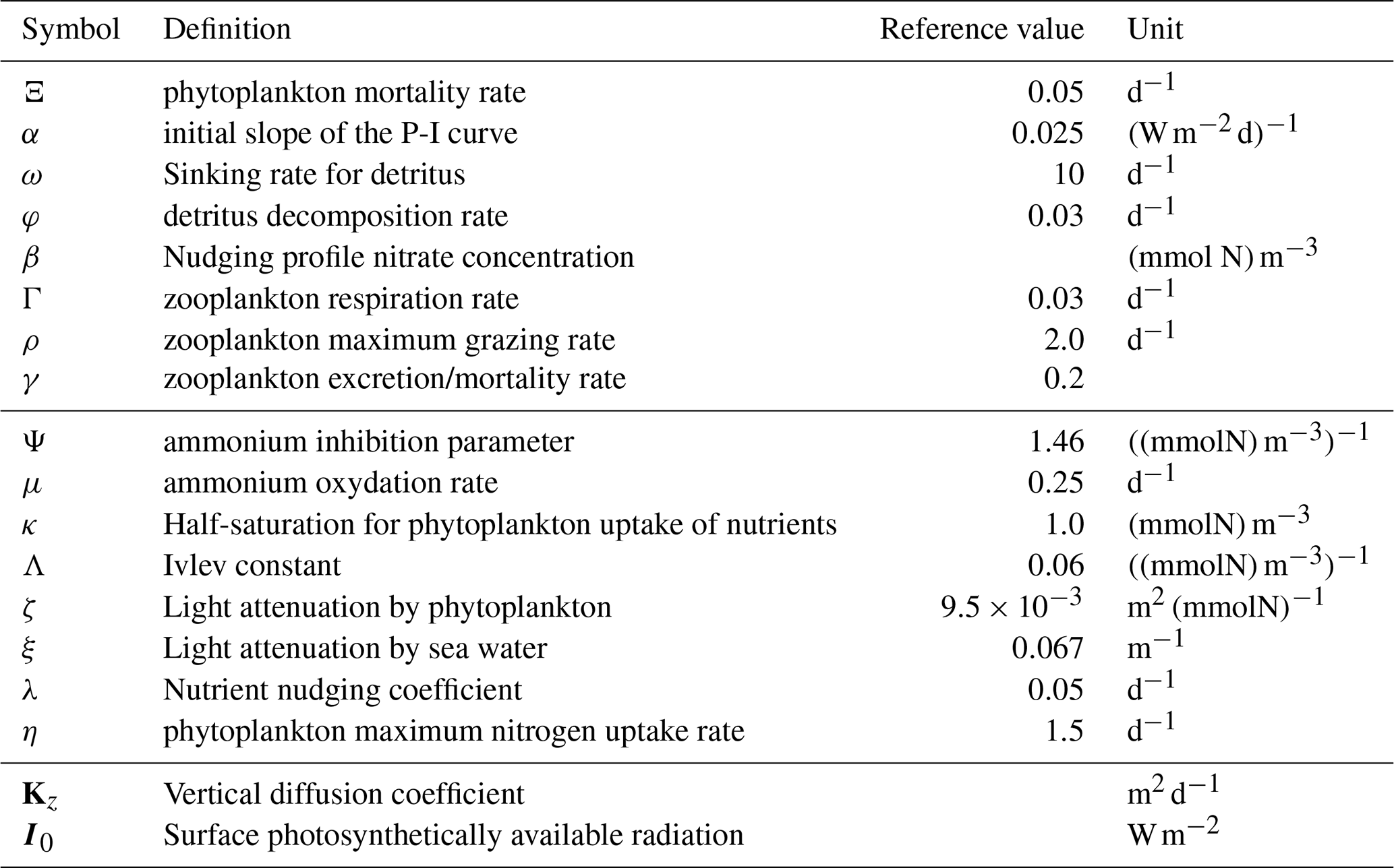
Following Newberger et al. (2003), we derive reference parameter values as detailed in Table 1. We tuned some parameters to ensure realistic nitrogen stock dynamics for the specified area for each compartments, especially a spring phytoplankton bloom, followed by a detritus peak and a subsequent zooplankton peak. Furthermore, it is preferable to avoid excessive P–Z oscillations with respect to prey-predator coupling.

2.2 Ocean physics and BGC datasets

Regarding the physical forcings in (Eq. 2), we use the realistic North Atlantic subpolar gyre simulation (Le Corre et al., 2020) spanning 7 years from 1 January 2002 and 31 December 2008 with a resolution of 2 km. This simulation is based on the CROCO model, which was developed from the Regional Ocean Modelling System (ROMS, Shchepetkin and McWilliams, 2005). We under sample from this simulation a set of 1-year time series of the solar irradiance I₀ and of vertical ocean mixing profiles K_z, that we loop over 3 years in order to achieve a seasonal steady state. I₀ has a 12 h time resolution and a 0.25° horizontal resolution, while K_z has a daily time resolution and a 40 km horizontal resolution. We focus on the upper ocean layer between sea surface and 350 m deep with 35 sigma vertical levels. Our study area is a 5°×5° box centred at the PAP (Porcupine Abyssal Plain) station in the North Atlantic ocean, where numerous studies are ongoing to better understand the carbon export processes in the meso-pelagic layer (Chevillon et al., 2026; Johnson et al., 2024; Baker et al., 2022; Bagniewski et al., 2011). Overall, the resulting 1D dataset is composed of 1-year time series $\mathit{\left\{}{\mathit{I}}_{\mathrm{0}}\right(t,p),\forall t\in {\mathrm{\Omega }}_t\mathit{\}}$ and $\mathit{\left\{}{\mathbf{K}}_z\right(t,p),\forall t\in {\mathrm{\Omega }}_t\mathit{\}}$ defined in a time space Ω_t at a horizontal location p∈Ω_p.

For a given physical forcing time series, we run ocean BGC simulations according to model 2.1. For each simulation, we uniformly sample model parameters in a ±20  % range of their reference value (see Table 1). Each simulation includes a 2-year period of spin-up (w.r.t. Appendix C) with a constant nitrogen concentration as initial condition, fixed to β for NO₃ and 1  % of β for the other compartments. As detailed in Sect. 2.1, β is defined according to the maximum annual mixed layer depth with respect to the mean vertical pattern of NO₃ concentration in the PAP area taken from the World Ocean Atlas 2023 (Garcia et al., 2024). Overall, these ocean BGC simulations result in 3100 sets of 1-year daily sampled time series for the five BGC compartments.

Typically 3100 simulations (so called OSSEs) are available, of which card(Ω_train)=2000 are used for training, card(Ω_valid)=1000 for validation, of the learning based scheme (presented in Sect. 3.3). The remaining card(Ω_test)=100 datasets are reserved to test each calibration method.

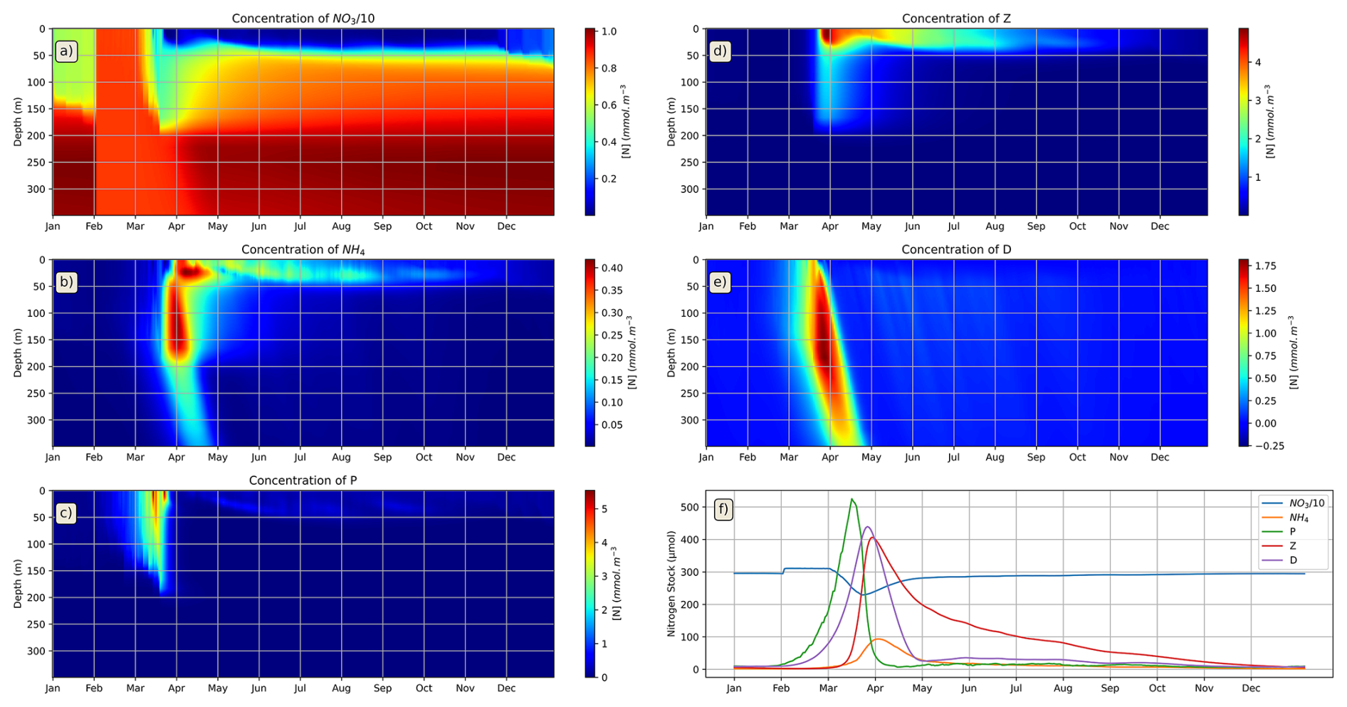
Figure 1 Hovmöller plot representing the nitrogen concentration between the surface and a depth of 350 m over the course of a year. The plot includes nitrate (a), ammonium (b), phytoplankton (c), zooplankton (d), and detritus (e). The integrated nitrogen stocks are represented (f) throughout the year as well for each BGC states.

2.3 Simulated physical forcing uncertainties

We augment our dataset with noisy physical forcings to account for the uncertainties observed in ocean reanalysis dataset (Lellouche et al., 2021). It is widely acknowledged that state-of-the-art global ocean reanalyses cannot resolve upper ocean dynamics for horizontal scales below one hundred kilometres (Ballarotta et al., 2019; Drillet et al., 2014). Given the impact of fine-scale physical ocean dynamics onto biogeochemical ones (Picard et al., 2024; Lévy, 2008; McGillicuddy et al., 1998), these uncertainties likely affect the calibration and reanalysis of ocean BGC dynamics using assimilation-based approaches. To simulate such uncertainties and biases in our dataset, we proceed as follows. Let us consider a given location at sea surface p and a time t and the associated physical forcings $\mathbf{U}(t,p)=\left(\begin{array}{c}{\mathit{I}}_{\mathrm{0}}(t,p)\\ {\mathbf{K}}_z(t,p)\end{array}\right)$. We define the noisy physical forcings ${\mathbf{U}}^{*}(t,p)$ at space-time location (t,p) as:

$$\begin{array}{}\text{(3)}& {\mathbf{U}}^{*}(t,p)=\mathbf{U}\left(t,p+v\left(t\right)\right)\end{array}$$

where v is a random time-evolving process stated as a first-order linear bivariate Gaussian auto-regressive process (Lai and Lu, 2017) with standard deviation σ_v. The term v accounts for a spatial location uncertainty (Ballarotta et al., 2019; Drillet et al., 2014). The definition of the noisy forcings in (Eq. 3) involves a spatial interpolation using a linear interpolation for both vertical mixing and solar irradiance. We consider three uncertainty levels: σ_v=0.15° (Level 1), σ_v=0.25° (Level 2) and σ_v=0.5° (Level 3). We point out that the considered spatial uncertainty is 95  % of spatial shifts within ±2σ_v of the reference location. The interpolated profiles U(t,p) and ${\mathbf{U}}^{*}(t,p)$ denote vectors that represent surface irradiance and vertical mixing values throughout the entire water column.

The resulting physical error patterns can be interpreted as misplaced mesoscale-to-submesoscale features (Escudier et al., 2021; Storto et al., 2019) seen in current physical reanalyses, depending on space-time range of the spatial shift (here, up to 0.5°). Due to the fine-scale variability in the input physical fields, especially for vertical ocean mixing profiles, they can include mean biases, amplitude shifts, changes in the vertical profiles. We acknowledge that this procedure cannot reproduce large-scale uncertainties and biases which may be observed in global reanalyses (Boucher et al., 2020).

2.4 Simulated observation configurations

Besides physical forcing uncertainties, we also assess the impact of observation configurations onto calibration and reanalysis performance. We may distinguish two main categories of observing systems for ocean BGC processes: scientific cruises, BGC ARGO floats. These two categories differ in the associated space-time sampling.

Scientific studies sample specific areas and provide samples, as the Bermuda Atlantic Time-series Study (BATS) (Steinberg et al., 2001; Phillips and Joyce, 2007) that uses conductivity, temperature, depth sensors (CTD, Williams, 2009) or bottles on rosette for specific analyses in order to detect specific temporal dynamics. The associated time sampling may typically range from days to months. The BGC ARGO network provides a global observation network, where each float delivers at a 10 d sampling rate vertical ocean profiles with a high vertical resolution, usually a few metres, of key variables, including among others temperature, salinity, oxygen, fluorescence, backscattering (a proxy for particle), and lately nitrate (Claustre et al., 2020; Gould et al., 2013). Across these different observing systems, some compartments are easier to monitor than others. Especially, zooplankton and ammonium concentrations are notoriously difficult to estimate and require substantial installations to be deployed (Everett et al., 2017), ammonium being measured from water sampling and zooplankton from nets (or cameras for micro-zooplankton, Picheral et al., 2010). By comparison, the assessment of nitrate, phytoplankton, and detritus concentrations is easier using proxies, such as chlorophyll-A for phytoplankton (directly measured from water fluorescence, Zeng and Li, 2015), or sensors directly measuring these parameters, such as ultraviolet sensors for nitrates (Pidcock et al., 2010). Overall, the resulting different observation configurations result in different space-time sampling patterns. Through the 1D ocean BGC setup considered setup, this study focuses on regular time sampling patterns from days to a month as well as the following four observation configurations for the water column:

• Strategy 0 – Perfect scenario: As a baseline scenario, we assume the 5 compartments to be observed for the whole water column.

• Strategy 1 – CTD + Rosette: inspired by scientific cruise sampling using CTD/Rosette system (Gould et al., 2013), this scenario assumes nitrate, phytoplankton and detritus to be measured at every depth level, while ammonium and zooplankton concentrations are measured only at the specific depths where the Rosette bottles are closed, i.e., at 5, 25, 50, 100, 150, 200 and 350 m.

• Strategy 2 – CTD: this strategy considers only the CTD-based observations described above in Strategy 1, such that no observations are available for ammonium and zooplankton.

• Strategy 3 – Rosette: this strategy considers only the Rosette-based sampling in Strategy 1, i.e., the 5 compartments measured at only 7 depth levels, namely at 5, 25, 50, 100, 150, 200 and 350 m.

All observation configurations account for a zero-mean Gaussian additive measurement noise and a spherical covariance matrix with the following parameterization for the compartment-wise standard deviation, respectively 0.001, 0.0005, 0.04, 0.12, 0.08 (mmol m⁻³) for NO₃, NH₄, P, Z and D.

3 Methods

3.1 Problem Statement

We introduce the following notations. Hereafter, index i refers to a time index according to a discrete set of I+1 time steps $\mathit{\{}{t}_{\mathrm{0}},t_{\mathrm{1}},\mathrm{\dots },t_i,\mathrm{\dots },t_I\mathit{\}}$ such that $\forall i,t_{i+\mathrm{1}}=t_i+\mathit{\delta }t$. Similarly, index j refers to an index along the ocean depth dimension according to a discrete set of vertical levels $\mathit{\{}{z}_{\mathrm{0}},z_{\mathrm{1}},\mathrm{\dots },z_j,\mathrm{\dots },z_J\mathit{\}}$. Bolded variables, e.g. X, Y and U, refer to two-dimensional tensors according to time and depth, while a state at a specific time and depth is referred to as x(t,z). Especially, we denote ${\mathbf{X}}_{i,j}=\mathbf{x}(t_i,z_j)$ that represents the value of tensor X at time t_i and depth z_j. In addition ${\mathbf{X}}_i=\mathbf{x}\left(t_i\right)=({\mathbf{X}}_{i,\mathrm{0}},\mathrm{\dots },{\mathbf{X}}_{i,J})$ refers to the vector of depth-related values of X at time t_i.

Now, the calibration of a model consists in fitting observed fields to predicted ones by adjusting variables such as the model parameters or the initial state. In this case, the focus is on a BGC model, characterised by θ BGC parameters, which dynamic is represented by ODEs (see Eq. 2). The operator ℳ_θ(.) describes the dynamic of the system states from initial state conditions X₀ and forcings $\mathbf{U}=\mathit{\left\{}\mathbf{U}\right(t,z){\mathit{\}}}_{{\mathrm{\Omega }}_t,{\mathrm{\Omega }}_z}$ with Ω_t and Ω_z the time and spatial spaces that are considered. Especially, the time space (resp. spatial space) can be subdivided into T time steps (resp. H spatial steps) equally separated by a fixed period δt (resp. a fixed distance δz), such that ${\mathrm{\Omega }}_t=\mathit{\{}{t}_{\mathrm{0}},\mathrm{\dots },t_{T-\mathrm{1}}\mathit{\}}$ and $t_{i+\mathrm{1}}=t_i+\mathit{\delta }t,\forall i\left[\right[\mathrm{0},T\left[\right[$ (resp. ${\mathrm{\Omega }}_z=\mathit{\{}{z}_{\mathrm{0}},\mathrm{\dots },z_{H-\mathrm{1}}\mathit{\}}$ and $z_{j+\mathrm{1}}=z_j+\mathit{\delta }z,\forall j\left[\right[\mathrm{0},H\left[\right[$). The observation of some ocean states is assumed with an observation operator ℋ(.) that stands for the spatio-temporal sampling, and associated observation noise ϵ_obs. The variable Y denotes the observed states at different time steps. It is assumed that X and Y both have the same dimensions but ${\mathbf{Y}}_{i,j}=\mathrm{0}$ if the state is not observed at time t_i and depth z_j. Typically, ℋ is a diagonal matrix with a value of 0 for the non-observed states. The observation noise ϵ_obs features the various stochastic biases inherent to the observation processes. The system can thus be formulated as follows:

$$\begin{array}{}\text{(4)}& \left\{\begin{array}{l}x(t+\mathrm{1})={\mathcal{M}}_{\mathit{\theta }}\left(x\right(t),u(t\left)\right)\\ y\left(t\right)=\mathcal{H}\left(x\right(t\left)\right)+{\mathit{ϵ}}_{\mathrm{obs}}\end{array}\right.\end{array}$$

The calibration problem can be regarded as an inverse problem. The objective is to design an operator that maps BGC parameters to the available information, i.e., Y, U^* and θ_b (BGC parameters prior), to the actual BGC parameters θ. As mentioned in the introduction, particular attention is paid to the sparsity of the data, which can be formulated through ℋ(.). Moreover, we note ${\mathbf{U}}^{*}=\mathbf{U}+{\mathit{\nu }}_{\mathbf{U}}$ the available forcing data, with U the actual forcings and ${\mathit{\nu }}_{\mathbf{U}}=\mathit{\{}{{\mathit{\nu }}_{\mathbf{U}}}_{\mathrm{0}},\mathrm{\dots },{{\mathit{\nu }}_{\mathbf{U}}}_{k-\mathrm{1}}\mathit{\}}$ representing the spatio-temporal uncertainties. As generally assumed in assimilation or forecast problems, the considered forcings are U^* since exact forcings U are not available (Park et al., 2018; Guiavarc'h et al., 2019). In this study, the problem at stake is a joint calibration that aims to calibrate the model parameters, correct the forcings and reconstruct the BGC dynamics. In particular, the objective is to get an operator, denoted by 𝒦(.), s.t. $\left(\widehat{\mathit{\theta }},\widehat{\mathbf{X}},\widehat{\mathbf{U}}\right)=\mathcal{K}({\mathit{\theta }}_b,\mathbf{Y},{\mathbf{U}}^{*})$. The notations $\widehat{\mathit{\theta }}$, $\widehat{\mathbf{X}}$ and $\widehat{\mathbf{U}}$ respectively refer to estimated BGC parameters, reconstructed states and corrected forcings.

The complexity of a BGC model directly correlates with the difficulty of constraining it. The correlation of its parameters and the redundancy of the observations can result in certain parameters compensating for each other, leading to erroneous values: the system is under determined (Ward et al., 2013). A preliminary sensitivity test has been conducted in order to consider only sensitive parameters in the calibration with observed BGC state concentration. In other words, the calibration is based on only 8 out of the 16 BGC parameters, with the remaining 8 being assumed to be known (see Appendix B).

3.2 Data assimilation: 4Dvar method

Among the state-of-the-art data assimilation (DA) methods, this study proposes the variational data assimilation scheme as a reference calibration method (Pasquier et al., 2023; Park et al., 2018; Kane et al., 2011; Brasseur et al., 2009; Berline et al., 2007). This weakly constrained 4Dvar scheme (Fablet et al., 2021b; Frerix et al., 2021; Trémolet, 2007) seeks to identify an optimal set of BGC parameters θ and initial states X_i, that minimises the error of BGC states simulation ℳ_θ(X_i,U_i), based on a set of observation data Y (Eq. 5). We consider ocean states at times $\mathit{\{}{t}_{\mathrm{0}},\mathrm{\dots },t_{T-\mathrm{1}}\mathit{\}}$ over a period Tδt. In addition, the period Tδt can be divided into d sub-periods of Δ time steps, such that dΔδt=Tδt (see Fig. 2). The weakly constrained nature of the 4Dvar scheme accounts for a dynamic error. This error is handled by dividing the studied time series into sub-windows (here we consider sub-windows of Δ time steps) and by ensuring the model accuracy over these short simulated periods. For this, we denote ${\mathit{X}}_{\mathrm{0}}^{d-\mathrm{1}}=({\mathit{X}}_{\mathrm{0}},{\mathit{X}}_{\mathrm{\Delta }},\mathrm{\cdots },{\mathit{X}}_{(d-\mathrm{1})\mathrm{\Delta }})$ as the state at the first time step of the d Δδt-time windows. In the same way, ${\mathit{X}}_{\mathrm{1}}^{d-\mathrm{1}}=({\mathit{X}}_{\mathrm{1}},{\mathit{X}}_{\mathrm{\Delta }+\mathrm{1}},\mathrm{\cdots },{\mathit{X}}_{(d-\mathrm{1})\mathrm{\Delta }+\mathrm{1}})$ refers to the second time step of the d Δδt-time windows.

$$\begin{array}{}\text{(5)}& \mathcal{J}(\mathbf{X},\mathbf{Y},\mathbf{U})={\mathcal{J}}_{\mathrm{obs}}(\mathbf{X},\mathbf{Y},\mathbf{U})+{\mathcal{J}}_{\mathrm{model}}(\mathbf{X},\mathbf{U})\end{array}$$

The primary right-hand side term of the variational cost is a fundamental component in variational methods, ensuring that model simulation aligns with observed states (defined in Eq. (7) and illustrated as Err_obs in Fig. 2). Each (Δ−1)-time step of each Δδt-time window is simulated and compared to the observed state when it is available. We denote by ${\mathcal{M}}_{\mathit{\theta }}^{\left(i\right)}({\mathit{X}}_{\mathrm{0}},{\mathit{U}}_{\mathrm{0}:i-\mathrm{1}})={\mathcal{M}}_{\mathit{\theta }}\left({\mathcal{M}}_{\mathit{\theta }}^{(i-\mathrm{1})}({\mathit{X}}_{\mathrm{0}},{\mathit{U}}_{\mathrm{0}:i-\mathrm{2}}),{\mathit{U}}_{i-\mathrm{1}}\right)$ the application of the dynamical model operator ℳ(⋅) defined in Eq. (4) between step i−1 and step i. This notation facilitates the writing of simulated states over several time steps and leads to ${\mathcal{M}}_{\mathit{\theta }}^{\left(\mathrm{1}\right)}({\mathit{X}}_{\mathrm{0}},{\mathit{U}}_{\mathrm{0}})={\mathcal{M}}_{\mathit{\theta }}({\mathit{X}}_{\mathrm{0}},{\mathit{U}}_{\mathrm{0}})={\mathit{X}}_{\mathrm{1}}$. The simulation of BGC states X from time steps 0 to i, requires the initial state X₀ and forcings at each time step ${\mathit{U}}_{\mathrm{0}:i-\mathrm{1}}$. Thus, ${\mathit{X}}_i={\mathcal{M}}_{\mathit{\theta }}({\mathit{X}}_{i-\mathrm{1}},{\mathit{U}}_{i-\mathrm{1}})$ can be written as ${\mathit{X}}_i={\mathcal{M}}_{\mathit{\theta }}^{(i-\mathrm{1})}({\mathit{X}}_{\mathrm{0}},{\mathit{U}}_{\mathrm{0}:i-\mathrm{1}})$. Moreover we introduce the notation:

$$\begin{array}{}\text{(6)}& \begin{array}{rl}{\mathcal{M}}_{\mathit{\theta }}^{\mathrm{\Delta }-\mathrm{1}}\left({\mathit{X}}_i,{\mathit{U}}_{i:i+\mathrm{\Delta }-\mathrm{1}}\right)=& ({\mathcal{M}}_{\mathit{\theta }}^{\left(\mathrm{0}\right)}\\ & \left({\mathit{X}}_i,{\mathit{U}}_i\right),{\mathcal{M}}_{\mathit{\theta }}^{\left(\mathrm{1}\right)}\left({\mathit{X}}_i,{\mathit{U}}_{i:i+\mathrm{1}}\right),\\ & \mathrm{\cdots },{\mathcal{M}}_{\mathit{\theta }}^{(\mathrm{\Delta }-\mathrm{1})}\left({\mathit{X}}_i,{\mathit{U}}_{i:i+\mathrm{\Delta }-\mathrm{1}}\right))\end{array}\end{array}$$

that returns a matrix with the simulated states at each step from step 0 to step Δ. In combination with ${\mathbf{X}}_{\mathrm{0}}^{d-\mathrm{1}}$ (defined in Sect. 3.1) that gathers the state at the first time step of every Δδt-time period, the term ${\mathcal{M}}_{\mathit{\theta }}^{\mathrm{\Delta }-\mathrm{1}}({\mathbf{X}}_{\mathrm{0}}^{d-\mathrm{1}},{\mathbf{U}}_{\mathrm{0}:\mathrm{\Delta }-\mathrm{1}}^{d-\mathrm{1}})$ indicates the Δ simulated terms of each of the dΔδt-time periods. The notation $\left|\right|\mathbf{Y}|{|}_{{\mathbf{R}}^{-\mathrm{1}}}^{\mathrm{2}}$ product stands for Y^TR⁻¹Y, with R a covariance matrix relative to the observation noise. In our case R⁻¹ is a diagonal matrix with $[\mathrm{1}/{\mathit{\sigma }}^{\mathrm{2}}]$ as coefficients, σ the state error standard deviation.

$$\begin{array}{}\text{(7)}& {\mathcal{J}}_{\mathrm{obs}}(\mathbf{X},\mathbf{Y},\mathbf{U})={∥\mathcal{H}\left({\mathcal{M}}_{\mathit{\theta }}^{\mathrm{\Delta }-\mathrm{1}}({\mathbf{X}}_{\mathrm{0}}^{d-\mathrm{1}},{\mathbf{U}}_{\mathrm{0}:\mathrm{\Delta }-\mathrm{1}}^{d-\mathrm{1}})\right)-{\mathbf{Y}}_{\mathrm{0}:d\mathrm{\Delta }-\mathrm{1}}∥}_{{\mathbf{R}}^{-\mathrm{1}}}^{\mathrm{2}}\end{array}$$

The second right-hand side term, defined in Eq. (8), aims to constrain the time consistency of the BGC states for the successive time windows. Following an approach similar to a weak-constrained 4DVar scheme, this measures the model error between a state X_(k+1)Δ and the BGC states simulated from the Δ previous time steps, i.e., ${\mathcal{M}}_{\mathit{\theta }}^{\left(\mathrm{\Delta }\right)}\left({\mathit{X}}_{k\mathrm{\Delta }},{\mathit{U}}_{k\mathrm{\Delta }:(k+\mathrm{1})\mathrm{\Delta }}\right)$.

$$\begin{array}{}\text{(8)}& {\mathcal{J}}_{\mathrm{model}}(\mathbf{X},\mathbf{Y},\mathbf{U})={∥{\mathcal{M}}_{\mathit{\theta }}^{(\mathrm{\Delta }-\mathrm{1})}\left({\mathbf{X}}_{\mathrm{0}}^{d-\mathrm{1}},{\mathbf{U}}_{\mathrm{0}:\mathrm{\Delta }-\mathrm{1}}^{d-\mathrm{1}}\right)-{\mathbf{X}}_{\mathrm{\Delta }}^{d-\mathrm{1}}∥}_{{\mathbf{B}}^{-\mathrm{1}}}^{\mathrm{2}}\end{array}$$

with B the model error covariance. We consider a diagonal covariance matrix whose diagonal terms ${\mathbf{B}}_{C,C}={\mathit{\tau }}_{\mathrm{DA}}{{\mathit{\sigma }}_C}^{\mathrm{2}}$, where ${{\mathit{\sigma }}_C}^{\mathrm{2}}$ denotes the variance associated with BGC state C. The coefficient τ_DA is a positive scalar that controls the relative weight of the observation and model costs in Eq. (5). Based on cross-validation experiments, we set ${\mathit{\tau }}_{\mathrm{DA}}={\mathrm{10}}^{-\mathrm{3}}$ for all our experiments.

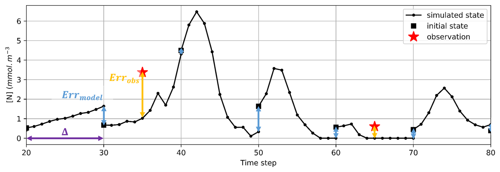
Figure 2 The following illustration is provided to demonstrate the two error terms of the variational cost (cf. Eq. 5) of a time-varying field. The state is simulated over Δ time steps (delineated in purple) from initial state (black square) and is assessed through two aspects. The observation error (Err_obs in orange) is indicative of the discrepancy between a simulated state (black dot) and an observed state (red star). The model error (Err_model in blue) is indicative of the error relative to the consistency of the model over a range of Δ time steps.

Numerically speaking, it is assumed to have the adjoint operator or a differentiable implementation of the model ℳ w.r.t. parameters and states. Then we solve the above minimization with a fixed-step gradient descent, beginning with a first guess of the BGC parameters and the initial states as illustrated Fig. 3. The minimization process typically involves 1000 gradient descent steps, implemented using an Adam optimizer. The assimilation process entails optimising the BGC initial conditions, which are not directly observable. In this case, we use as a first guess a constant matrix with the mean value of the state over the time and spatial spaces, i.e., X=1E[Y] the averaged observed states, with 1 a matrix full of 1. The BGC parameter first guess θ^b is a draw following the uniform distribution between 0.8 and 1.2 times the reference value of the parameter (cf. Table 1), s.t. ${\mathit{\theta }}^b\sim \mathcal{U}(\mathrm{0.8}\times {\mathit{\theta }}_{\mathrm{ref}},\mathrm{1.2}\times {\mathit{\theta }}_{\mathrm{ref}})$. Therefore, the control variables in this study are the BGC parameters θ and the initial state estimate ${\mathbf{X}}_{\mathrm{0}}^{d-\mathrm{1}}$ at the beginning of the d sub-periods. As commonly assumed in operational systems for biogeochemistry, forcings are assumed to be error-free, i.e., U=U_True. In other words, we assume the forcing uncertainty to be part of the model error covariance in the minimization process.

Among the variational methods, ensemble variational methods enable to consider various members of a distribution simultaneously. Here, we consider an ensemble of L realizations of noisy forcings ${\mathbf{U}}^{\left(l\right)*}=\stackrel{\mathrm{‾}}{\mathbf{U}}+{{\mathit{\nu }}_U}^{\left(l\right)}$ for each sample, with $l\in \left[\right[\mathrm{1},L\left[\right[$ the number of the member and $\stackrel{\mathrm{‾}}{\mathbf{U}}$ the mean forcings. Assuming the forcing uncertainty distribution is centred on 0 (Bannister, 2017), i.e., $\frac{\mathrm{1}}{L}{\sum }_l{{\mathit{\nu }}_U}^{\left(l\right)}=\mathrm{0}$, the noisy forcings U^* is non-biased, and $\frac{\mathrm{1}}{L}{\sum }_l{\mathbf{U}}^{\left(l\right)*}=\frac{\mathrm{1}}{L}{\sum }_l(\stackrel{\mathrm{‾}}{\mathbf{U}}+{{\mathit{\nu }}_U}^{\left(l\right)})=\stackrel{\mathrm{‾}}{\mathbf{U}}$. Especially, one could consider solving the calibration problem for this estimated mean forcing, i.e. $\left(\widehat{\mathit{\theta }},\widehat{\mathbf{X}}\right)={\sum }_l{\mathcal{K}}^{\mathrm{DA}}({\mathit{\theta }}_b,\mathbf{Y},{\mathbf{U}}^{\left(l\right)*})={\mathcal{K}}^{\mathrm{DA}}({\mathit{\theta }}_b,\mathbf{Y},\stackrel{\mathrm{‾}}{\mathbf{U}})$.

3.3 Learning-based method: UNet

In this paper, we propose a neural-based scheme as an alternative to DA. The method delineates the calibration problem as the supervised learning of a neural mapping between inputs, i.e., observations and forcings, and model parameters variables. As illustrated in Fig. 4, we benefit from the versatility of deep learning schemes to jointly address the calibration problem, the denoising of the forcings as well as the reconstruction of the BGC dynamics. Formally, the neural network acts as an operator $(\widehat{\mathit{\theta }},\widehat{\mathbf{U}},\widehat{\mathbf{X}})={\mathcal{K}}^{\mathrm{NN}}({\mathit{\theta }}_b,\mathbf{Y},{\mathbf{U}}^{*})$ with Υ as the parameters of the neural network using the notations introduced in Sect. 3.1.

For the training of neural operator 𝒦^NN, we assume a representative dataset gathering error-prone and error-free forcings, BGC parameters, true BGC dynamics and associated observation data. The training phase amounts to minimizing the following loss with respect to neural network parameters Υ:

$$\begin{array}{}\text{(9)}& \mathcal{L}\mathcal{O}\mathcal{S}\mathcal{S}=\sum \left(a(\widehat{\mathit{\theta }}-\mathit{\theta }{)}^{\mathrm{2}}+b(\widehat{\mathbf{U}}-\mathbf{U}{)}^{\mathrm{2}}+c(\widehat{\mathbf{X}}-\mathbf{X}{)}^{\mathrm{2}}\right)\end{array}$$

with a, b, and c weighing factors for the three MSE terms, namely the BGC model parameters, the forcings and the BGC states. We tune the value of these parameters empirically through cross-validation experiments according to a=1, b=5, and c=5. Our training configuration exploits a stochastic gradient descent method using an Adam optimizer with a learning rate of $\mathrm{1}\times {\mathrm{10}}^{-\mathrm{3}}$ and mini-batches of size 256.

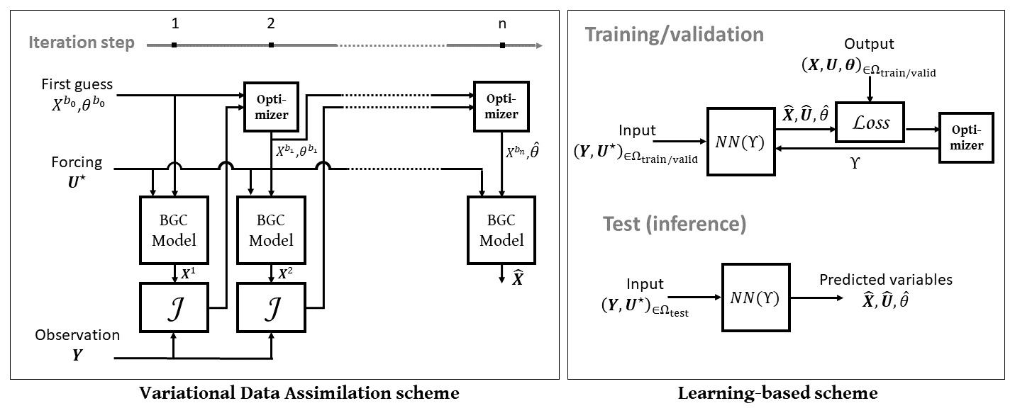
Figure 3 The following sketch illustrates the two calibration schemes. The variational data assimilation scheme (left panel) constrains the BGC parameters and initial states during a regression process. From a first guess upon the states X^b and the BGC parameters θ^b and forcings U^* the method iteratively reconstructs the states from the BGC model, computes the variational cost with the observation and performs a gradient descent over the guesses through an optimizer. The learning-based calibration scheme (right panel) employs a neural network (NN) with parameters Υ that are trained and validated prior to being tested. In the course of the training process, the NN employs observation, denoted by Y and spurious forcings, denoted by U^* to predict states, denoted by $\widehat{\mathbf{X}}$, forcings $\widehat{\mathbf{U}}$ and BGC parameters $\widehat{\mathit{\theta }}$, which are evaluated through the ℒ𝒪𝒮𝒮 function, which returns a value employed by the optimiser to modulate the NN parameters Υ. The training, the validation and the test steps involve three totally independent datasets, respectively labelled Ω_train, Ω_valid and Ω_test.

Regarding the neural architecture, we consider a state-of-the-art UNet (Ronneberger et al., 2015). This multi-scale architecture is widely used in imaging applications (Liu et al., 2020) including for ocean studies (Luo et al., 2023; Smith et al., 2023; Roussillon et al., 2023; Ducournau and Fablet, 2016). The computational graph of the architecture is illustrated in Fig. 4. More complex architectures, combining for instance UNet with residual and attention mechanisms (Zhang and Yin, 2024; Wang et al., 2024), could be considered. We favoured the trade-off between computational efficiency and computational complexity in our experiments. The model is composed of a central block (ensemble of layers) with a contracting (encoding) path for the capture of relevant features of the input and a symmetric expanding (decoding) path that enables precise localization of these features. We complement the classic UNet architecture with three task-specific blocks which address the estimation of BGC parameters, BGC states and physical forcings. We use a channel-wide normalization of the inputs and outputs according the mean and standard deviation of each variable. This ensures effective training of the model and equitable assessment of the estimated variables. The preprocessing also includes the space-time interpolation and concatenation of the observed state and the physical forcings. The input results in a tensor of dimension ($N_{\mathrm{batch}}\times (N_{\mathrm{ch}}\times (N_z+\mathrm{1}\left)\right)\times \mathrm{2}{N}_T$), where N_batch is the number of samples per batch. N_ch=7 is the number of channels, i.e., the number of state compartments (5 for NO₃, NH₄, P, Z, D) and the number of forcings (2 for K_z and I₀). N_z=34 is the number of layers at which tracers are resolved (vertical diffusion is computed at the interfaces, i.e., at $N_z+\mathrm{1}=\mathrm{35}$ depths), and N_T is the time-window length in days (since the forcings are provided at 12 h intervals).

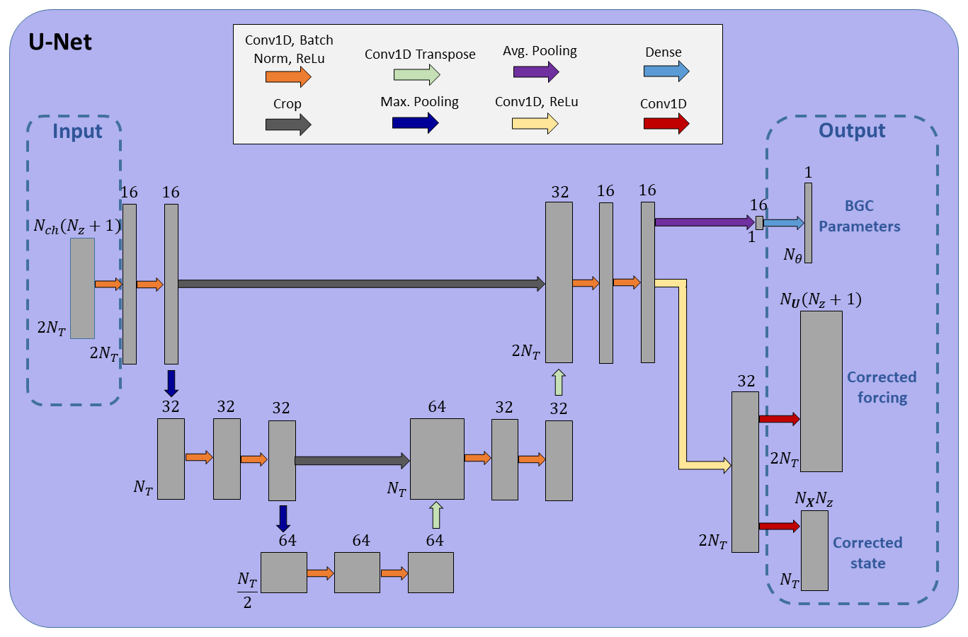
Figure 4 Computational graph of the UNet architecture. The model is composed of a main block of layer, itself composed of an encoding part

3.4 Hybrid approach: ML + DA

The learning-based method, described above, simultaneously estimates the parameters, the initial BGC conditions, and the physical forcings. As shown in preliminary experiments (see Appendix D), the DA-based method produced more accurate parameter estimates than the UNet in error-free physical configurations. These findings suggest the potential benefit of an hybrid approach, as sketched in Fig. 5, combining both the UNet and 4Dvar frameworks. This hybrid scheme operates in two stages, starting with the UNet (presented in Sect. 3.3). Its outputs–namely the BGC parameters, the BGC state variables, and the physical forcing–are then passed as inputs to the 4Dvar method. The parameters and BGC state estimated by the UNet serve as a first guess for the assimilation process, while the UNet-derived physical fields are used as forcings. We expect the subsequent data assimilation step to refine model parameters and the BGC state, owing to the expected smaller errors in the physical forcings and the use of first guesses that are closer to the true state.

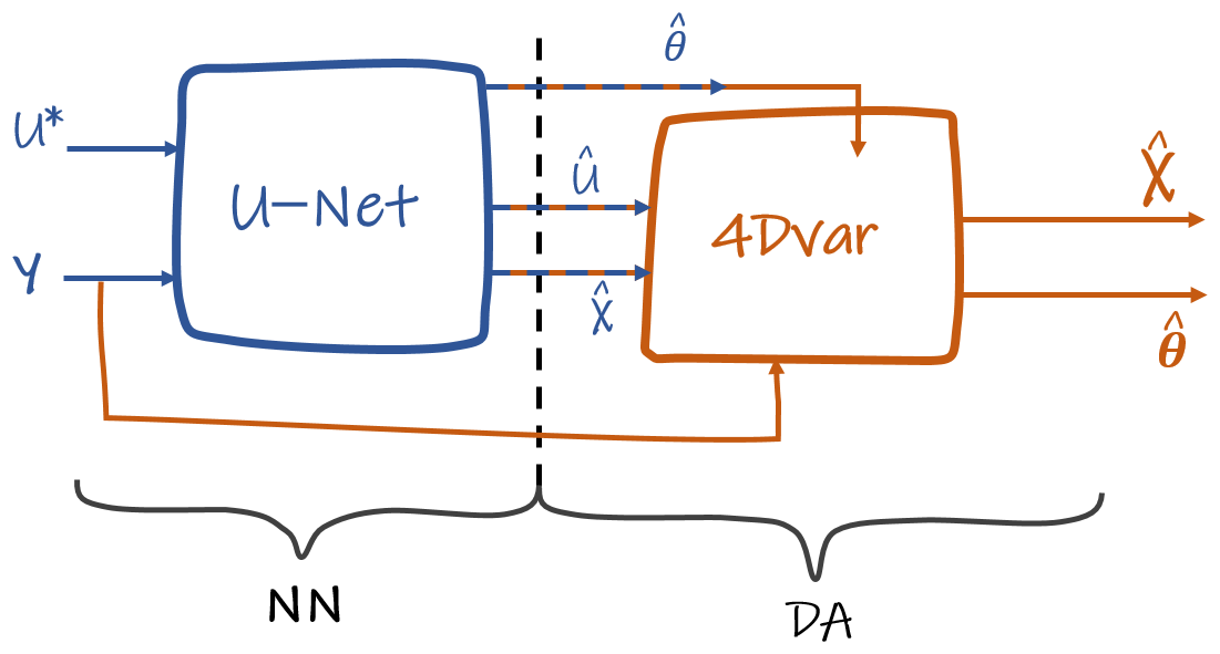
Figure 5 Diagram of the hybrid scheme showing input and output variables. A UNet model takes observed BGC state components and physical forcing as input to infer BGC parameters, and to correct and interpolate BGC state components and physical forcing. The UNet-derived BGC parameters and state components are then used as the initial guess in a 4Dvar scheme, together with the corrected physical forcing, to further adjust the BGC state and parameters in the final output.

3.5 Evaluation framework

In this section, we describe our evaluation procedure for both the targeted model calibration problem as well as the reconstruction of the physical forcings and of the ocean BGC dynamics. Specifically, we detail how each scenario is considered and the metrics used to compare the three schemes: the 4Dvar DA scheme, the UNet scheme and a hybridization of the two methods.

Two categories of metrics are considered: those computed in the space of BGC model parameters, and those defined from BGC state dynamics. The first set of metrics involves statistics (e.g., mean, standard deviation…) and normalized error values for each BGC model parameter, expressed as $\frac{\mathit{\theta }-\widehat{\mathit{\theta }}}{\stackrel{\mathrm{‾}}{\mathit{\theta }}}$, where $\stackrel{\mathrm{‾}}{\mathit{\theta }}$ is the mean value of the parameter (given in Table 1), θ is the true parameter value, and $\widehat{\mathit{\theta }}$ is the estimated value. For the second category of metrics, we proceed as follows. Given a predefined dataset of error-free forcings and initial conditions, we simulate a pair of BGC state time series according to Eq. (2) using the estimated and true BGC model parameters and focus on depth-integrated quantities to assess the difference between any such pair. Let us denote by ${\mathit{S}}_c\left(t\right)={\int }_{{\mathrm{\Omega }}_z}\mathbf{c}(t,z)\mathrm{d}z$ for the depth-integrated stock of a tracer of concentration c at time t (see Fig. 1f).

Given the stock S_c(t) for the true BGC model parameters and the stock ${\mathit{S}}_{\widehat{c}}\left(t\right)$ for the estimated ones, we define the following three metrics:

• The correlation, computed as corr$\left({\mathit{S}}_c\left(t\right),{\mathit{S}}_{\widehat{c}}\left(t\right)\right)$, evaluates the pattern of the estimated stock.

• The shift, computed as $\arg {max}_{\mathrm{d}t}\left\{\mathrm{corr}\left({\mathit{S}}_c\left(t\right),{\mathit{S}}_{\widehat{c}}(t+\mathrm{d}t)\right)\right\}$, measures the temporal shift of the stock dynamics.

• The amplitude, computed as $\mathrm{2}\times \frac{max\left({\mathit{S}}_c\right)-max\left({\mathit{S}}_{\widehat{c}}\right)}{max\left({\mathit{S}}_{\widehat{c}}\right)-min\left({\mathit{S}}_{\widehat{c}}\right)+max\left({\mathit{S}}_c\right)-min\left({\mathit{S}}_c\right)}$, quantifies the accuracy of the estimated stock bloom ratio. If the estimated stock ${\mathit{S}}_{\widehat{c}}$ is over estimated compared to the actual stock S_c, the metrics tends to a value of 2, whereas with an under estimated stock, the metric tends to 0.

We compute these three metrics for each BGC state, i.e., NO₃, NH₄, P, Z and D. We focus on the period between the beginning of February and the end of May, when the BGC dynamics are at their strongest, as shown Fig. 1. For each forcing and observation scenario, we consider an evaluation dataset of card(Ω_test)=100 samples. For each sample of this evaluation dataset, we assume the physical forcings to be given as an ensemble of L=10 members (see Sect. 3.2). We then run the considered calibration and reanalysis scheme for each member of the physical forcing ensemble. The ensemble mean and standard deviation provide us with final estimates of BGC model parameters and of their uncertainties, from which we compute the different metrics described above. In addition to the ensemble mean and standard deviation, we also assess how well the ensemble distribution encompasses the ground truth, referred to as its “distribution representativeness”. This metric quantifies the proportion of true state values lying within the 95 % ensemble interval, i.e., the fraction of true concentrations c(t,z) that falls inside $\left[{\mathit{\mu }}_{\widehat{c}}(t,z)-\mathrm{2}{\mathit{\sigma }}_{\widehat{c}}(t,z),{\mathit{\mu }}_{\widehat{c}}(t,z)+\mathrm{2}{\mathit{\sigma }}_{\widehat{c}}(t,z)\right]$ over all times and depths. Here, ${\mathit{\mu }}_{\widehat{c}}(t,z)$ and ${\mathit{\sigma }}_{\widehat{c}}(t,z)$ denote the ensemble-mean and ensemble-standard-deviation of the concentration estimate at time t and depth z, respectively.

For the corrected forcings $\widehat{\mathbf{U}}$, we consider two evaluation metrics: the NMSE with respect the true forcings U and the relative improvement with respect to the noisy forcings computed as $\mathbb{E}\left[\right(\widehat{\mathbf{U}}-\mathbf{U}{)}^{\mathrm{2}})/({\mathbf{U}}^{*}-\mathbf{U}{)}^{\mathrm{2}}]$. The latter is reported in % and equals 100 % when the corrected forcing error has the same order of magnitude than the initial error and 0 % if the correcting forcing perfectly matches the true one.

4 Results

This section presents our numerical experiments. We first perform a comparative analysis of the performance of the DA-based and learning-based schemes for a reference observation and uncertainty scenario (Sect. 4.1). We then focus on a sensitivity analysis with respect to forcing uncertainties and observation sampling scenarios (Sect. 4.2 and 4.3). We also report an evaluation of the performance for the ocean BGC reanalysis problem (Sect. 4.4).

4.1 Comparative evaluation of data-assimilation-based and learning-based calibration schemes

We report in Fig. 6 the evaluation of the two calibration schemes presented in the Sect. 3.2 and 3.3 for a reference scenario. This scenario corresponds to the lowest uncertainty level (Level-1 uncertainty scenario, i.e. 0.3° of spatial uncertainty in the physical forcings as described in Sect. 2.3) and the CTD + Rosette observation strategy (Strategy 1 cf. Section 2.4) with a 10 d sampling rate. This reference scenario is rather optimistic compared to the characteristics of operational systems (Clements et al., 2022; Cossarini et al., 2019; Bagniewski et al., 2011; Berline et al., 2007).

Figure 6a–c shows the distribution of the correlation, shift and amplitude ratio metrics between the nitrogen stock obtained from the calibrated BGC parameters and the actual BGC parameters, for 100 different 1D simulations. The correlation score results in a clear shift towards lower values for the DA-based scheme with a mean correlation score of 0.88 and a minimum value of −0.49 compared to a mean value of 0.99 and a minimum at 0.68 for the UNet. We observe a consistency of the two approaches with better correlation values for NH₄ and Z compared to NO₃, P and D. As depicted in Fig. 6b, the resulting stocks in the NH₄, P, Z and D compartments are commonly shifted, up to 10 d for the UNet and up to 28 d for the 4Dvar method. Figure 6c illustrates that the predicted stocks are more often under-estimated or over-estimated when using the parameters from the DA-based scheme. This is supported by a larger standard deviation of the amplitude ratio for the DA-based scheme compared to the learning-based approach (0.28 vs. 0.08).

Figure 6d presents the normalized error of the estimated parameters (defined in Sect. 3.5). While the DA-based approach leads to parameter estimate error between −0.38 and 0.40, the UNet reaches lower error values between −0.20 and 0.18. On average, it reduces the estimation error standard deviation by a factor of 2.8. As expected, some BGC parameters such as ρ, Γ and β show a lower estimation uncertainty compared with the other parameters consistently for the two calibration schemes. This likely relates to differences in the identifiability of BGC model parameters. Unsurprisingly, parameters γ, Ξ and ω, which drive mortality (of P and Z) and particle sinking processes, are known to be under-constrained in classic model-based frameworks (Mamnun et al., 2022; Beck et al., 2017). Importantly, the learning-based scheme depicts much lower differences of the calibration uncertainties across model parameters.

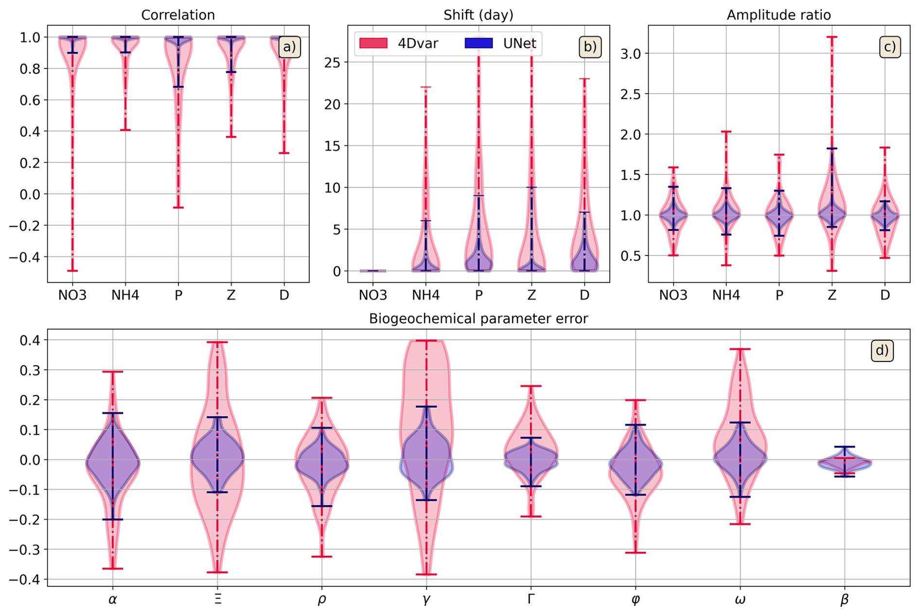
Figure 6 Evaluation metrics of the calibration of the BGC model. We assess a 4Dvar DA scheme (red distribution) and a learning-based scheme (blue distribution). We considered the following metrics: the correlation (a), the shift (b), the amplitude ratio (c) and the parameter estimate error (NME) (d) as detailed in Sect. 3.5. We plot the distribution of the metrics for an evaluation dataset of 100 1D BGC simulations. We consider a baseline scenario given by low-level forcing uncertainties (case-1 scenario in Sect. 2.3) and a CTD + Rosette observation configuration with a 10 d sampling (Strategy 1 in Sect. 2.4).

Based on the quantitative evaluation presented previously, in the subsequent sections, we focus on the learning-based calibration scheme to study the impact of physical forcing uncertainties and observation configurations into the calibration performance.

4.2 Impact of physical forcing uncertainties onto calibration performance

Here, we assess the impact of physical forcing uncertainties onto the performance of the ocean BGC model calibration using the learning-based approach. As discussed in Sect. 2.3, a sensitivity analysis is conducted for three distinct scenarios, designated as case-1, case-2 and case-3 corresponding respectively to mean horizontal uncertainties of 0.3, 0.5 and 1° in (Eq. 3). The observation configuration involves a 10 d sampling of the full BGC state over a 120 d period from February to June. The evaluation dataset comprises 100 samples, each sample being associated with an ensemble of 10 noisy forcings. For each sample, we consider the ensemble mean as the estimated BGC parameters for both the DA-based and learning-based schemes. We report in Fig. 7 the synthesis of these experiments.

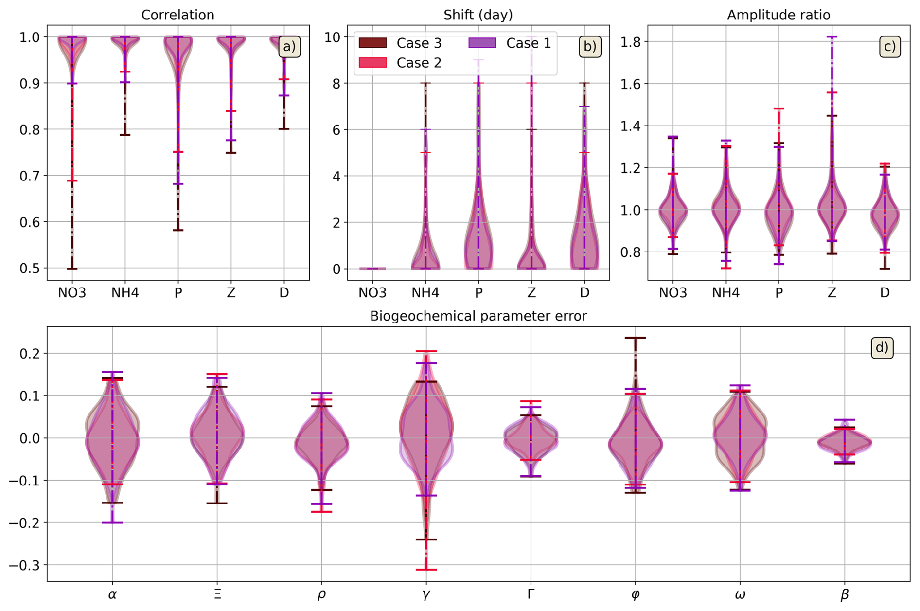
Figure 7 Evaluation metrics of the learning-based calibration of the BGC model with respect to forcings' uncertainties. We consider the same metrics as in Fig. 6 with the same evaluation dataset of 100 1D BGC simulations. We compare the distribution of the metrics for three scenarii with increasing forcings' uncertainty levels: namely, case-1 (purple distribution), case-2 (red distribution) and case-3 (brown distribution) as described in Sect. 2.3. These experiments rely in the baseline observation configuration with a CTD + Rosette strategy and a 10 d time sampling (see Sect. 2.4).

Figure 7 reports the calibration performance of the learning-based scheme for the three forcing uncertainty scenarii introduced in Sect. 2.3. Overall, the performance does not show a strong dependence on the uncertainty level. The averaged correlation scores ranges between 0.98 and 0.99 with larger values for NH₄ stocks. The shift scores have close standard deviations with larger lags for P and D stocks. Finally, all the amplitude scores feature the same distribution whatever the considered scenario or state. With regard to the BGC parameter errors illustrated in Fig. 7d, similar patterns are observed. The standard deviation of parameters varies by less than 0.05 for all forcing uncertainty levels. Parameters α, γ and φ however demonstrate a heightened degree of sensitivity. The standard deviation values range between 0.01 and 0.017 in the three scenarii under consideration. For the remaining parameters, the standard deviation does not vary by more than 0.007 between the scenarios.

4.3 Impact of the observation scenarii onto calibration performance

As described in Sect. 2.4, we carry out experiments to evaluate the sensitivity of the calibration performance with respect to the observation configurations, using the learning-based approach. As depicted Fig. 8, we first focus on the impact of the time sampling rate assuming a CTD + Rosette observation configuration for the vertical profiles. We recall that the CTD + Rosette configuration involves observations of NO₃, P and D concentrations at all vertical levels and of NH₄ and Z concentrations at 5, 25, 50, 100, 150, 200 and 350 metres deep. The four scenarios differ in terms of the time sampling rate: 60 d (brown distributions in Fig. 8), 30 d (red distributions in Fig. 8), 10 d (purple distributions in Fig. 8) and 1 d (blue distribution in Fig. 8). As illustrated in Fig. 8a–c, the correlation, shift and amplitude ratio metrics demonstrate a marked difference for sampling rates of 1 and 10 d vs. 30 d and 60 d. For instance, we observe high values of the correlation score (resp. 0.994 and 0.987) for 1 and 10 d sampling rates, compared to 0.97 and 0.957 for 30 and 60 d sampling rates. Similarly, the average of the shift score remains below 0.66 d for a sampling up to 10 d and is above 1.10 from a 30 d sampling. As the time sampling increases from 1 to 60 d, the amplitude ratio standard deviation concomitantly rises, reaching 0.05, 0.08, 0.13 and 0.14, respectively. Regarding BGC parameter error in Fig. 8d, the standard deviation increases with the sampling period, with values of 0.03, 0.05, 0.09 and 0.10 recorded for time sampling rates from 1 to 60 d. Some parameter depicts a greater sensitivity to the observation sampling rate. For instance, parameter Γ exhibits a steep increase to 0.1 of the standard deviation for the 60 d scenario, whereas for 1, 10 and 30 d, the standard deviation remains between 0.02 and 0.06. It is noteworthy to mention that parameters Ξ, φ and ω have the same error distribution whether the states are observed every 30 d or every 60 d. As illustrated in Fig. 1, the simulated BGC trajectories typically involve a one-peak pattern with a duration of a few weeks for each tracer. Therefore, 30 and 60 d sampling rates likely poorly inform the duration and the amplitude of the peak. As an illustration, we report in Fig. 9 a scatterplot of the NMSE of BGC parameters vs. the NMSE of the reconstruction of the BGC state from an interpolation of the observations. The 30 and 60 d sampling configurations clearly result in both high estimation errors for BGC parameters and of the reconstruction error, the latter being regarded as a proxy of the quality of the monitoring of the peak-shaped pattern of the BGC states.

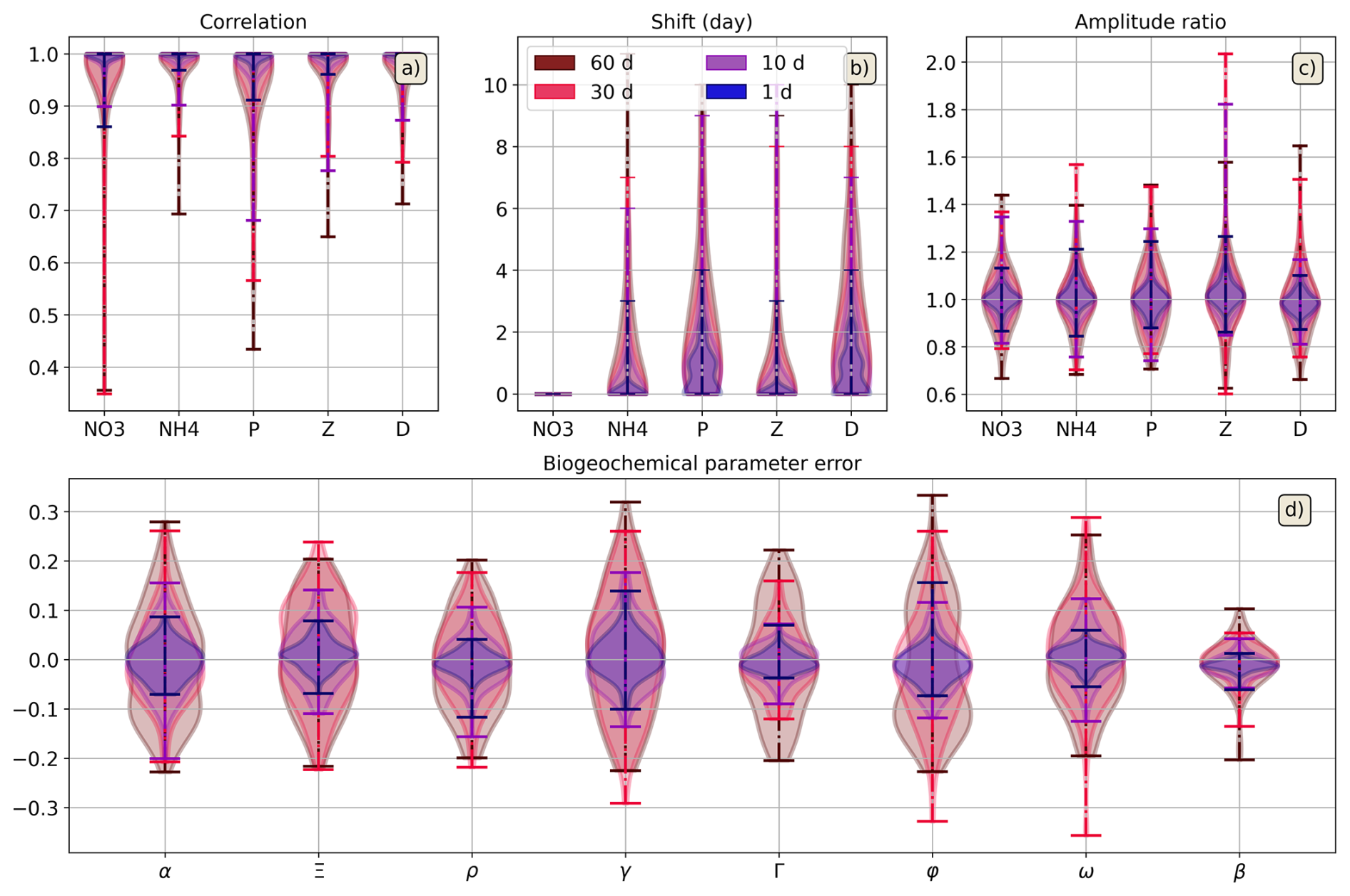
Figure 8 Evaluation metrics of the learning-based calibration of the BGC model with respect to time sampling. We consider the same metrics as in Fig. 6 with the same evaluation dataset of 100 1D BGC simulations. We compare the distribution of the metrics for four scenarii with varying time sampling: namely, daily state sampling (dark blue distribution), 10 d state sampling (purple distribution), 30 d state sampling (red distribution) and 60 d state sampling (brown distribution) as described in Sect. 2.4. These experiments rely in the baseline Case-1 forcings' uncertainties and a CTD + Rosette observation configuration (see Sect. 2.3 and 2.4).

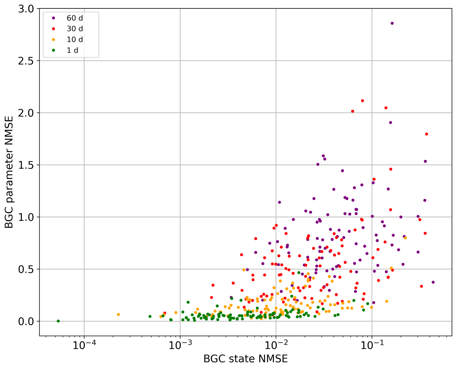
Figure 9 Scatterplot of the estimated BGC parameter NMSE according to the NSME of the input BGC states. Each dot features the aforementioned NMSEs of one sample among the 100 considered for a daily sampling (green), a 10 d sampling (yellow), a 30 d sampling (orange) or a 60 d sampling (purple) scenario. For these scenario the space sampling goes with respect to a CTD + Rosette-like strategy and Case-1 forcings' uncertainties.

Besides the time sampling rate, we also assess the impact of the sampling pattern along the depth dimension according to the following four strategies: an ideal scenario in which each state is sampled at all depths (light blue distribution), the CTD sampling strategy (red distribution), the Rosette sampling strategy (brown distribution) and the CTD + Rosette sampling strategy (purple distribution). All of the aforementioned scenarios are described in Sect. 2.4. All experiments exploit here a 10 d sampling rate. The first scenario serves as a baseline to assess an upper bound of the calibration performance. As illustrated in Fig. 10, there is a clear lowering of the calibration performance when considering the CTD-only and Rosette-only strategies compared to a “All obs” observation configuration. Among the different BGC states, we observe the largest impact for NO₃ and P in Fig. 10a–c. Figure 10a–c underline lower reconstructed states correlation, especially for NO₃ with a score value of 0.98, as compared to 0.99 for the 'all obs' configuration. It is noteworthy that the standard deviation is four to five times higher in the latter case. It is also observed that there is a marginal increase in delay for every reconstructed stock except NO₃. Shifts are 0.3 to 0.5 d higher for CTD-only and Rosette-only configurations in comparison with a “all obs” configuration. Regarding BGC parameter errors, Fig. 10d strengthens the discrepancy between the CTD-only and Rosette-only observation configuration for ρ, γ, Γ and φ when compared to an idealised scenario. The former scenarii exhibit a range of errors that is 1.4 to 3.5 times higher than the “all obs” scenario, and a range of standard deviation values that is 1.5 to 3.9 times higher.

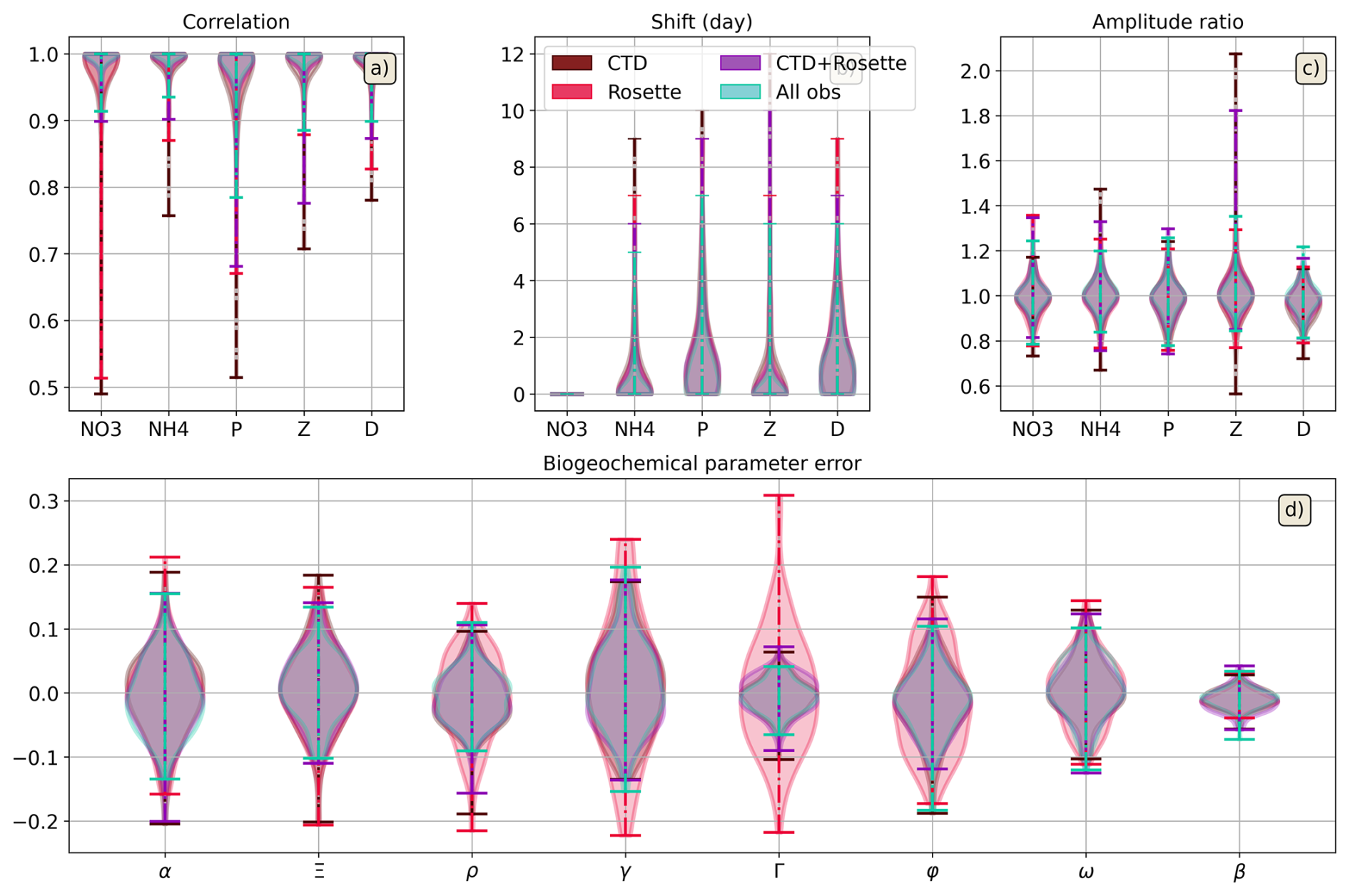
Figure 10 Evaluation metrics of the learning-based calibration of the BGC model with respect to forcing uncertainties. We consider the same metrics as in Fig. 6 with the same evaluation dataset of 100 1D BGC simulations. We compare the distribution of the metrics for four scenarii with varying vertical sampling: namely, strategy 0 – All obs. (light blue distribution), strategy 1 – CTD + Rosette (purple distribution), strategy 2 – CTD (red distribution) and strategy 3 – Rosette (brown distribution) as described in Sect. 2.4. These experiments rely in the baseline Case-1 forcings' uncertainties and a 10 d time sampling (see Sect. 2.4).

4.4 Reanalyses of BGC dynamics under partial observations and noisy forcings

We also evaluate the potential impact of the proposed calibration schemes onto the reconstruction of the 1D BGC dynamics when considering forcing uncertainties and a realistic observation configurations. We focus on the baseline scenario used in Sect. 4.1 to benchmark the DA-based and learning-based calibration schemes (we also report a complementary experiment involving unobserved components is presented in Appendix E). As described in Sect. 3.2 and 3.3, both approaches considered lead to the estimation of the time series of the BGC states. Furthermore, learning-based schemes also yield a corrected version of the forcings. This suggests the consideration of the third hybrid approach, presented in Sect. 3.4. It should be noted that, unlike the experiment described in Sect. 4.1, the BGC parameters are not treated as control variables in the DA scheme. This choice is based on a preliminary experiment (reported in Appendix F), which shows that the hybrid method cannot reliably optimize both the BGC parameters and the BGC state variables simultaneously, due to a low robustness to physical forcings, which are not corrected with sufficient accuracy by Unet. Consequently, the hybrid scheme focuses on refining the BGC state trajectories.

Table 2 synthetizes the results of these experiments. The performance of the reconstructions is assessed through the NMSE of the five BGC variables. For the three approaches that have been benchmarked, ensemble-mean estimates are derived using the reconstructions issued from each of the ten forcing members (see Sect. 3.5). Similarly to the calibration experiments, the findings indicate a substantial impact of forcing uncertainties on the performance of the DA-based approach, with two to three times higher NMSE values observed in comparison to the learning-based scheme (e.g., 0.012 vs. 0.007 and 0.241 vs. 0.084 for NO₃ and P). It is noteworthy that the hybrid approach enhances the reconstruction performance for all BGC variables with the exception of NO₃. For instance, the NMSE is divided by two for P and Z concentrations (respectively 0.085 vs. 0.047 and 0.017 vs. 0.008). It is also important to note that this reconstruction performance significantly improves a direct interpolation of the observation data (e.g., 0.029 vs. 0.769 in average). Regarding the standard deviation, presented in Table 2 and computed from the 10-member ensembles for each sample, the learning-based scheme provides the lowest uncertainty for P, Z and D concentrations and the UNet based scheme provides the lowest uncertainty for reconstructed NO₃ and NH₄ concentrations. The hybrid method provides the highest standard deviation, i.e. a larger distribution within the 10-member ensembles. According to the distribution representativeness, the hybrid scheme yields the distribution that least underestimates physical uncertainties, resulting in a more realistic overall distribution. The former method results in a distribution that comprises 80.6 % of the true value, in comparison to 42.1 % and 65.8 % for the DA-based and the learning-based schemes, respectively.

Table 2 Table of the NMSE, standard deviation and representativeness of the reconstructed BGC states error, for the three presented schemes: a 4Dvar-only-based scheme, a UNet-only-based scheme and a hybrid scheme. The bold values refer to the lowest NMSEs and the highest 'Distribution representativeness' within the three methods. The mean error is computed over the 10 members of the 100 samples for each BGC state. The standard deviation is computed from the 10-member ensemble of normalised reconstructed states and then averaged among the 100 samples. The representativeness of the data is indicated by the percentage of points of the true state that are comprised within the confidence interval of the distribution of the reconstructed state.

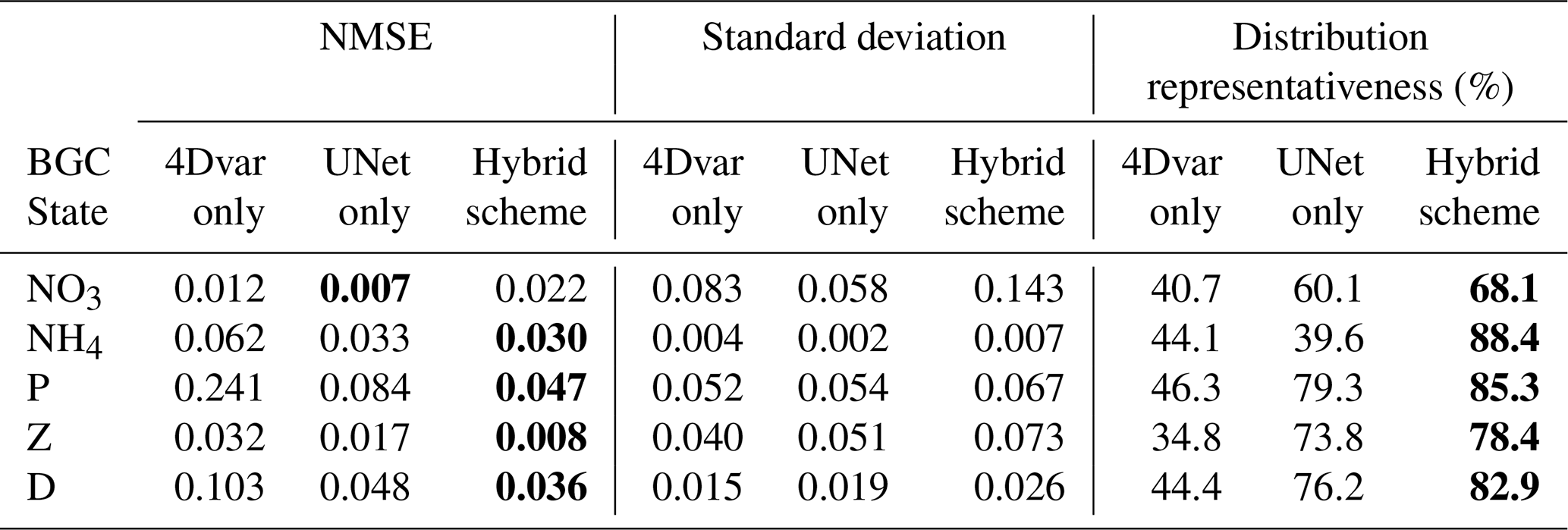
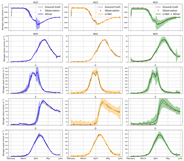
Figure 11 illustrates one sample (i.e. one 10-member ensemble) among the 100 presented in Table 2, representative of the average performance of the currently presented experiment (other samples are available in Appendix G). The following comparison is made of the reconstructed BGC stocks using a 4Dvar-only-based (blue), a UNet-only-based (orange) and a hybrid (green) scheme on one sample, and their relative uncertainty space is denoted as the space between the lower limit of the μ−2σ and the μ+2σ. As demonstrated by the latter figure, the reconstruction performance of each state is satisfactory for every reconstruction scheme, provided that the initial guess is a noisy 10 d linear interpolation of the observed states (red dots). Especially, the methods provide a relatively accurate representation of the bloom event, which occurs between April and May. Furthermore, it displays the uncertainty time evolution of the different reconstruction schemes. The uncertainty related to the DA-based schemes tends to be higher during the bloom period, with some bulging shapes, that is attributable to the 10 d division of the reconstructed period. This uncertainty remains constant (approximately ±30 mmol m⁻²) throughout the entire reconstructed period with the UNet-based scheme. The hybrid method also yields uncertainty estimates that combine characteristics of the last two methods: they are larger during the bloom period, similar to the DA-based reconstruction scheme, while remaining as smooth as the uncertainties obtained with the UNet-reconstructed stocks. Overall, we obtain higher uncertainty levels that more effectively encompass the true state values.

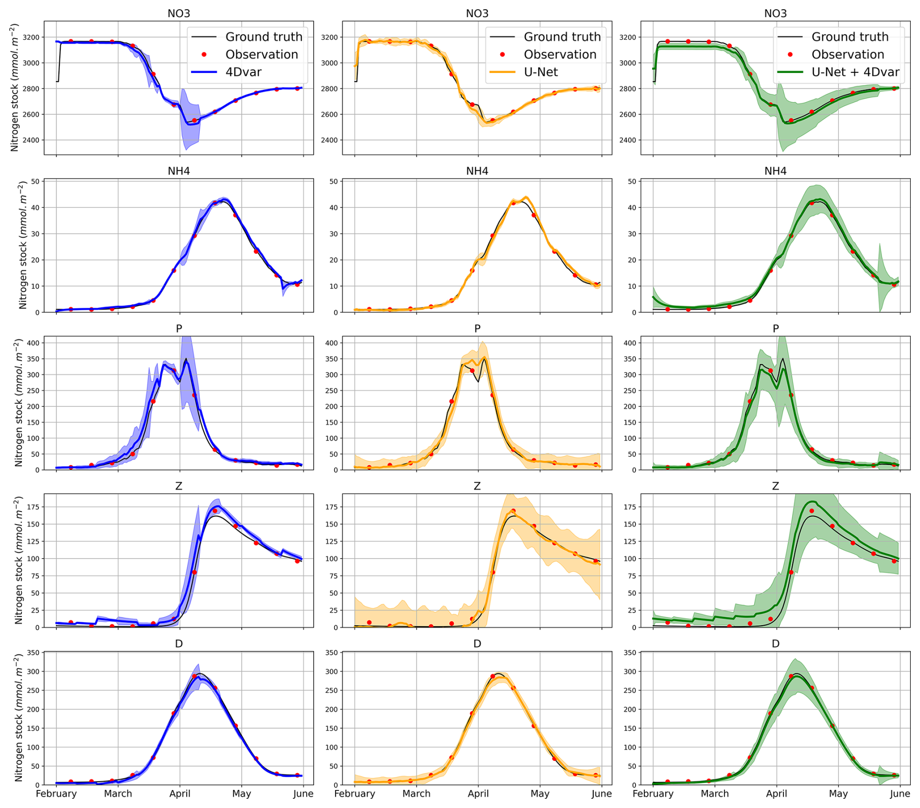
Figure 11 Reconstructed stocks associated with the five BGC states: NO₃, NH₄, P, Z and D; for one ensemble using a DA-based scheme (blue), a UNet-based scheme (orange) and a hybrid UNet+4DVar base scheme (green), w.r.t. a scenario of case 1 forcing uncertainty, states observed with a 10 d time sampling and a CTD + Rosette-like sampling strategy. The bold line indicates the mean stock among the 10-member ensemble, with the uncertainty, i.e., the mean value ±2σ with σ being the standard deviation of the 10 members. The aforementioned confidence interval is associated with the colourized shape. The ground truth is represented by the black curve. The observed states are denoted by red dots.

5 Discussion

This section discusses our main findings regarding the potential contribution of learning-based schemes to the calibration and reanalysis of ocean BGC dynamics. In particular, we address key challenges to deploy these methodologies on real observation datasets and state-of-the-art 3D ocean BGC models.

5.1 A learning-based scheme to improve ocean BGC simulations under spurious forcings

The proposed solution supports the relevance of learning-based schemes to enhance biogeochemical simulation in spite of spurious physical forcings. The calibration of ocean BGC models is among the major sources of uncertainties in simulating, forecasting and reanalysis ocean BGC dynamics (Gehlen et al., 2015; Kriest et al., 2010). State-of-the-art systems generally rely on data assimilation approaches and expert knowledge (Singh et al., 2025; Ford, 2021; Kaufman et al., 2018; Dowd et al., 2014; Kane et al., 2011; Song et al., 2016; Losa et al., 2004; Faugeras et al., 2003). This approach achieves better calibration performance relative to a state-of-the-art learning-based technique when physics is perfectly known, as demonstrated for a 0D framework in Littaye et al. (2025b) and here for a 1D framework (see Appendix D). Nevertheless, these results remain valid in an idealised, error-free setting. In realistic applications, the method may become computationally expensive and highly sensitive to uncertainties in ocean physics and limited observation configurations. This has prompted researchers to investigate alternative approaches. The exploitation of learning-based methods has gained significant interest in ocean science. They have shown promise in uncovering key processes from noisy data (Gottwald and Reich, 2021; Buongiorno Nardelli, 2020) as well as tackling inverse problems such as model calibration problems (Buchanan et al., 2025; Higgs et al., 2025; Gupta and Lermusiaux, 2023; Bolton and Zanna, 2019). This study contributes to this ongoing research and explores end-to-end learning schemes to enhance the representation of ocean BGC processes. We extend our previous work (Littaye et al., 2025b) to realistic 1D ocean BGC OSSE. The experimental setup provides an intermediate-complexity testbed. This enables a more precise evaluation of how uncertainties in ocean physics and the sampling patterns of observing systems influence the calibration of ocean BGC models.

This approach achieves superior calibration performance relative to a state-of-the-art learning-based technique when the physics are perfectly known, as demonstrated in experiments conducted in a 0D framework (Littaye et al., 2025b) and a 1D framework (see Appendix D). Nevertheless, these results remain valid in an idealised, error-free setting. In realistic applications, the method may become computationally expensive and highly sensitive to uncertainties in ocean physics and limited observation configurations.

Our experiments highlight a clear impact of forcing uncertainties on model calibration performance for a variational data assimilation scheme. Here, forcings' uncertainties as presented in Eq. (4) do not account for possible large-scale uncertainties and focus on small-scale processes, spanning horizontal scales from 1 to several tens of kilometres. This likely underestimates the uncertainties in real ocean physics reanalyses. At sea surface, current reanalyses (Lellouche et al., 2021; Taburet et al., 2019) typically resolve dynamics down to horizontal scales of about 1–2°, given the present configuration of satellite-derived observations (Ballarotta et al., 2019). As pointed out in previous studies (Pasquier et al., 2023; Fransner et al., 2020; Bagniewski et al., 2011; Doney et al., 2004), such uncertainty levels strongly degrade the calibration performance of variational data assimilation schemes, which implicitly assumes error-free forcings. In the worst-case scenarios, the resulting calibration can substantially distort estimates of BGC parameters and simulated BGC patterns. To deal with forcing errors, the model-based calibration scheme can introduce substantial biases into BGC parameter estimates. There are noticeable shifts of the seasonal blooms up to a month for phytoplankton and peak amplitudes for nutrients, zooplankton and phytoplankton can be misestimated by factors exceeding 1.5, even under low-uncertainty conditions (see Fig. 6). By contrast, the learning-based scheme reaches a greater robustness for all tested configurations. The improvement stems from the end-to-end learning strategy. The neural network is trained to handle both forcing uncertainties and sparse observation configurations using a training dataset of around 3000 samples. This supervised learning paradigm cannot be implemented with this classic variational DA scheme, given the offline resolution of the physical field. The latter setting resembles an unsupervised approach, where the variational cost (Eq. 5) acts as the training loss. These findings provide evidence that supervised learning paradigms can outperform unsupervised methods for model calibration problems. Future work could explore benchmarks between coupled data assimilation methods and learning-based approaches for ocean BGC model calibration. Since the computational cost of such studies is currently prohibitive for state-of-the-art Earth system models, the design of intermediate-complexity alternatives would be valuable (e.g., 1D or multi-layer-2D settings).

This study also highlights the impact of in situ sampling patterns on both calibration and reanalysis tasks. Several studies (Kriest et al., 2023; Bisson et al., 2018; Bagniewski et al., 2011) have documented the influence of data availability on BGC model calibration. Regarding the depth-wise sampling pattern the Rosette-like sampling configuration yields results comparable to those obtained from full-depth observations of the five modelled states as shown in Fig. 10. However, the CTD-like sampling scheme reveals a critical role for ammonium and zooplankton information in constraining BGC parameters. This result is consistent with earlier studies (Bagniewski et al., 2011; Faugeras et al., 2003), which emphasise the value of zooplankton data in BGC model calibration. The temporal frequency of the sampling is also a key consideration, as deploying specialised equipment such as Rosettes to collect specific BGC components is costly. Our results underscore a marked difference in calibration performance between 10 d and 30 d sampling intervals, with the latter producing poor estimates of BGC parameters. Consistent with the system's temporal variability and inertia – i.e., its characteristic seasonal bloom – the 10 d optimum agrees with the weekly sampling interval identified as sufficient by Skákala et al. (2023). Further studies could investigate the added benefit of including complementary observations, such as temperature, salinity, dissolved oxygen and pH, in model calibration (Bock et al., 2022; Wang et al., 2020; Roemmich et al., 2019). This involves increasing the complexity of the model, e.g. by incorporating the temperature dependence of parameters and integrating carbon components (Blackford and Gilbert, 2007).

While we point out the possible combination of the proposed neural schemes with a variational data assimilation to enhance the reconstruction of ocean BGC dynamics, the development of hybrid approaches jointly exploiting model-based and learning-based paradigms is an active research avenue in data assimilation. They can help addressing DA challenges such as adjoint model computation, model parameterisation, model error correction and computationally-efficient optimizers (Singh et al., 2025; Gottwald and Reich, 2021; Farchi et al., 2021b; Fablet et al., 2021b). Our future work will explore how such hybrid schemes could improve furthers the calibration, simulation and reconstruction of ocean BGC dynamics.

5.2 Limits of the application framework for the learning-based method

The ability of the proposed learning-based scheme to deal with physical forcing uncertainties is limited by how these uncertainties are accounted for in the training dataset. The principle of neural-based methods is to learn a mapping from an input space to an output space. Such methods are effective within the range of input-output relationships exhibited in the training data. Their performance is thereby constrained by this data and this generalisation performance beyond the distribution of the training dataset is a challenge (Hensman and Masko, 2015). This aspect requires the training data to closely represent the conditions expected at inference time. In our study, input-data interpolation has proven effective in accommodating different spatial and temporal observation strategies. However, the neural network's performance depends on the level of forcing uncertainties in the specific scenario as described in Sect. 2.3. The input-output relationships learned by the model then differ between models trained with level-1, level-2 and level-3 forcing uncertainties. This suggests that maintaining the same level of data quality is essential to ensure reliable performance between from training to inference. As physics products can be resolved at different horizontal scales with different model parametrisations (Lellouche et al., 2021; Ballarotta et al., 2019), the nature of any associated errors may also be subject to variation. It would be worth investigating whether a single model can accommodate different types of forcing errors to both extract valid signals and correct erroneous components from the BGC observed states. As presented in Roussillon et al. (2023), multi-mode networks effectively capture different modes in input data, such as region dependent processes. Similarly, several learning-based models trained on different types of physical errors could be combined.

DA-based methods can straightforwardly accommodate different observation datasets with prescribed noise levels. By contrast, the present learning-based approach involves training a neural scheme for each observation configuration – namely, specific sampling patterns and observation noise parameters – as shown in Figs. 7–10. For regional case studies, this assumption of constant noise is reasonably justified (Kane et al., 2011). Scaling this approach to larger spatial domains, however, naturally introduces spatial variability in BGC distributions as well as time-varying observation errors. In learning-based frameworks, it is standard practice to train on large ensembles of samples spanning a wide range of input distributions, thereby enhancing robustness to diverse density regimes (Sarr, 2023). The versatility of neural schemes also enables to consider additional input variables to account among others for the observation configuration (e.g., noise level, sampling patterns, observation types), uncertainty levels of forcing or ocean provinces (Roussillon et al., 2023; Tan et al., 2022; Martinez et al., 2020). This may result in an increase of the complexity of the considered neural architectures. But, one would expect such all-purpose architectures to reach similar performance that configuration-specific ones with a significantly greater generalization potential beyond the training datasets.

It is important to note that BGC model errors, which we do not account for in our OSSEs, could significantly affect the application on real observations. The neural network here is trained to retrieve BGC parameters for known equations that fully reproduce the observed states, apart from observation noise. The underlying model assumes that BGC model errors arise primarily from incorrect calibration of the parameters. Nonetheless, simulated BGC state errors can also result from erroneous BGC process formulations or from coarsely resolved scales (Fennel et al., 2022; Ward et al., 2013; Losa et al., 2004). Several studies have explored learning-based tools as a solution to predict unresolved processes (Farchi et al., 2021b; Bolton and Zanna, 2019; Bonavita and Laloyaux, 2020). The ability to separate modelled from unresolved processes, when combined to model calibration, offers a new perspective to account for model error more effectively. This is of particular relevance given the increasing complexity of the BGC models (Ward et al., 2013) and their computational cost. Such methods could enable calibration of both simple BGC models, such as the one described in Sect. 2, and more complex models as in Aumont et al. (2015); Yool et al. (2013); Baretta et al. (1995), by calibrating the relevant processes and correcting the unresolved components.

In this study, we assume that BGC states are directly observable. In real world experiments, nitrate and ammonium concentrations are measurable using sensors or bottle sampling (Johnson et al., 2013; Guo et al., 2024). However, phytoplankton, zooplankton and detritus are much harder to directly observe. Phytoplankton is typically inferred from chlorophyll-a and fluorescence measurements (Zeng and Li, 2015). Huot et al. (2007) demonstrate that BGC model calibration is influenced by the choice of phytoplankton proxy. Additionally, in-situ instruments such as Underwater Vision Profilers, nets and backscattering provide information within specific size ranges (Picheral et al., 2010; Wiebe and Benfield, 2003; Organelli et al., 2018; Dall'Olmo et al., 2009). However, these measurements represent only a fraction of actual zooplankton and detritus concentrations (Christiansen, 2016). More complex models can explicitly represent chlorophyll and partition zooplankton and detritus into size classes (Aumont et al., 2015). This approach mitigates proxy biases, but at the cost of increased model complexity. Bridging such schemes and the proposed learning-based framework is a challenge for future work.

5.3 Scaling up to real ocean BGC dynamics

Our study supports the relevance of the proposed learning-based schemes for the calibration and reanalysis of ocean BGC dynamics through numerical experiments for an intermediate-complexity 1D NNPZD case-study. These results naturally raise questions on the applicability of these approaches to real ocean BGC dynamics. As discussed in the following, we distinguish three main scientific challenges to scale up to real-world case studies: namely the generation of training datasets for real-world case-studies, accounting for real observing systems and dealing with the full range of space-time variabilities of ocean dynamics on a global scale.

Training datasets play a pivotal role in the performance of learning-based schemes (Weiss and Provost, 2003; Mukherjee et al., 2003). State-of-the-art neural schemes may require anywhere from thousands to billions of training samples, depending on the complexity of the task and the neural architecture (Götz et al., 2022; Chen and Lin, 2014). In line with image-to-image and signal-to-signal mapping approaches (Febvre et al., 2024; Martinez et al., 2020), this study demonstrates that relevant calibration and reanalysis neural schemes can be trained using a few thousand samples, each corresponding to a one-year time series. Importantly, the training dataset spans the full range of ocean BGC parameters, forcing conditions, associated uncertainties, and observation patterns. To our knowledge, no such simulation dataset is currently available for state-of-the-art 3D ocean BGC models. However, while the associated computational complexity remains affordable in the present 1D case study, it could become prohibitive when scaled up to state-of-the-art 3D ocean BGC models. For illustration, a one-year simulation of a $\mathrm{1}/\mathrm{4}\mathit{°}$ NEMO-PISCES configuration typically requires between 1200 and 2000 hCPU (Institut Pierre Simon Laplace (IPSL), 2018). Therefore, the generation of a training dataset of few thousands of training samples similar to that considered in the current study would represent a computational effort similar to running ensemble simulation over decades with an ensemble size of 100 members. The development of neural emulators of ocean models, which emerge for ocean physics, will likely provide a solution to address this computational bottleneck. To date, the development of emulators has been primarily focused on the physical components of the ocean. Dheeshjith et al. (2025); El Aouni et al. (2025) propose realistic representation of the global ocean circulation. These data-driven models represent a novel alternative to conventional ocean physical models. For ocean BGC dynamics, current demonstrations focus on specific integrated or sea surface variables, such as sea surface chlorophyll (Gow-Smith and Séférian, 2026; Rahpoe and Bernardello, 2025; Roussillon et al., 2023). Neural emulators for 3D ocean BGC are likely to emerge rapidly. Combined with ocean physics and atmosphere emulators, they would provide new means to transfer our study to realistic ocean BGC frameworks, both in terms of training datasets as well as in terms of fully-controlled benchmarks.

A second challenge that has been identified in the application of the framework to real-world case studies is the ability to exploit actual observational datasets, as pointed out in the previous section. While the proposed approach readily extends to known observation models, i.e., when the relationship between the observations and the ocean BGC states is explicitly defined, the application to observations, which do not directly relate to a BGC state variable, will require additional methodological developments. We may cite among others ocean colour products and sea surface chlorophyll (Groom et al., 2019), sediment traps (Smetacek et al., 1978) and isotopic tracer measurements (Laws, 2013). In this context, it could be beneficial to employ neural schemes trained to relate measured quantities and modelled variables, as explored in the processing of Argo float data (Amadio et al., 2024). Such neural schemes could also be integrated into the simulation process used to generate training datasets, thereby enabling the training of end-to-end neural schemes that map directly from the observation space to the model parameter space. In such methodologies, the ability to represent observational and modelling uncertainties will be key for applications to real observation datasets.

Another key challenge in ocean dynamics lies in accounting for the full spectrum of spatio-temporal variability, including those driven by climate change. In this study, we focus on a specific region of the North Atlantic. The literature recognises distinct ocean bioregions, each characterised by specific interactions between physical and biogeochemical processes (Bock et al., 2022; Reygondeau et al., 2013). Existing bioregion classifications could inform the development of region-specific data-driven models (Zhao et al., 2020; Reygondeau et al., 2018; Krug et al., 2017), similar to the approach adopted here; meanwhile, recent advances in deep learning demonstrate that neural architectures can scale effectively with task complexity (Roussillon et al., 2023). For instance, our experiments employ neural architectures with approximately 130 000 parameters. By contrast, state-of-the-art neural schemes in weather forecasting and computer vision typically comprise tens of millions to billions of parameters (Bi et al., 2023; Chen et al., 2023). Mechanisms – such as attention blocks (Yang et al., 2024) – provide robust means of modelling complex, context-dependent relationships, thereby enabling models to adapt to intricate dynamics. However, scaling up to more complex neural architectures is likely to require larger training datasets, underscoring the interconnected nature of the challenges discussed here.

6 Conclusions

This work highlights the effectiveness of a learning-based method for calibrating a BGC model that accounts for uncertainties in physical forcing. We implemented an NNPZD BGC model within a vertical (1D) framework, forced by PAR and vertical diffusion. This setup enabled the evaluation of the improvements of a learning-based calibration relative to a conventional 4D variational data assimilation scheme. To account for poorly resolved submesoscale physics in reanalyses, a spatio-temporal uncertainty was introduced by interpolating vertical profiles at time-varying, horizontally shifted positions. Although the results remain sensibly similar across uncertainty levels, a shift in calibration performance is observed for sampling frequencies ranging from ten days to one month within this specific BGC dynamics. This pseudo-realistic configuration serves as an intermediate step between a simplified experimental setup using synthetic data and a fully realistic framework based on actual observations.

The UNet (learning-based scheme) was found to outperform the 4Dvar-based calibration scheme under idealised conditions, when forcing uncertainties are considered. Subsequently, we further evaluated the learning-based calibration under scenarios with varying quality and availability of observed ocean states. The results obtained demonstrated the model's aptitude to retrieve the correct information from the observed BGC states and the uncertain physical forcings. This enables precise estimation of BGC parameters, correction of forcings and reconstruction of BGC states. However, reinjecting the UNet outputs (corrected forcings and estimated BGC states and parameters) into a the 4D-Var scheme further improved the reconstruction of the BGC states. This result demonstrates the efficacy of knowledge-informed methods in comparison to fully neural-based tools.

It is important to note that the method still relies on strong assumptions and operates within an idealised framework. The proposed model remains scenario-dependent and its applicability to a real-world cases requires further validation. This study provides a novel perspective on the use of hybrid tools for the comprehensive or partial calibration of models, particularly in filtering input information. In conclusion, this study presents a tool with potential applicability for other models and frameworks.

Appendix A: Nitrate profile in the studied area

For each simulation, nitrate nudging is applied during winter to restore the nutrient vertical structure. The target nitrate profile is a uniform concentration, whose value is determined from the curve shown in Fig. A1, as described in Sect. 2.1.

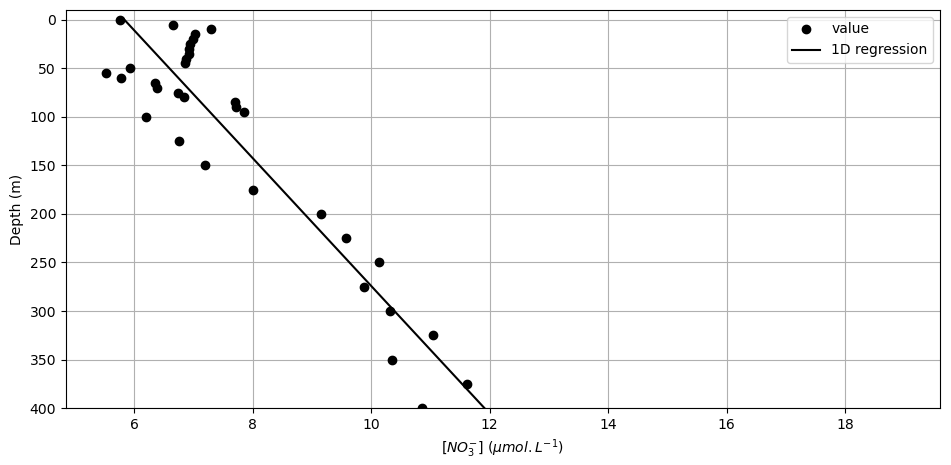
Figure A1 Nitrate vertical profile at the Porcupine Abyssal Plain (PAP) station. Monthly reanalysed nitrate data from Garcia et al. (2024) are shown for December, January, and February (dots), together with a first-order polynomial fit (line).

Appendix B: Sensitivity test of BGC parameters

Prior to the calibration experiments, a sensitivity test was conducted to evaluate the influence of each biogeochemical parameter. More precisely, the sensitivity of various metrics was assessed with respect to the perturbations in individual parameters. The analysis, summarised in Table B1, quantifies how variations in each parameter affect the resulting BGC dynamics. For each metric, a sensitivity coefficient s_m was computed as $s_{\mathrm{m}}=\frac{\frac{m^{+}-m^{-}}{m^{\mathrm{ref}}}}{\frac{{\mathit{\theta }}^{+}-{\mathit{\theta }}^{-}}{{\mathit{\theta }}^{\mathrm{ref}}}}$ where m⁺, m⁻, m^ref denote the values of metric obtained from simulations using the parameter sets θ⁺, θ⁻ and θ^ref, respectively. The notation θ_ref refers to the reference parameter values (see Table 1), with ${\mathit{\theta }}^{+}=\mathrm{1.01}\times {\mathit{\theta }}_{\mathrm{ref}}$, ${\mathit{\theta }}^{-}=\mathrm{0.99}\times {\mathit{\theta }}_{\mathrm{ref}}$.

Table B1 Table showing the sensitivity of biogeochemical (BGC) metrics to variations in BGC parameters. The evaluated BGC metrics include: phytoplankton bloom peak intensity, peak timing, and bloom duration; zooplankton bloom peak intensity and its time lag relative to the phytoplankton peak; the maximum sedimentation flux at 200 m; the maximum detritus concentration at 350 m; and the timing of this detritus maximum. Each metric is assessed with respect to the parameters listed in Table 1.

Appendix C: Spin-up justification

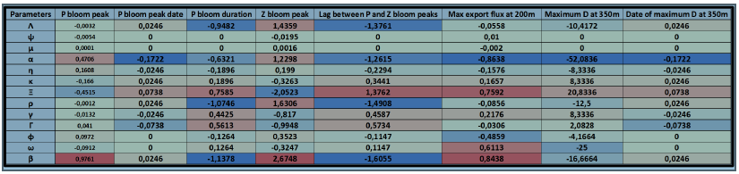
This study uses BGC simulations spanning several years, following a two-year spin-up period. Figure C1 illustrates the evolution of seasonal BGC simulations over five consecutive years, initiated from the same initial conditions adopted in our analysis. The resulting BGC stocks exhibit minor differences between the first two years, particularly for nitrate. In contrast, the third, fourth, and fifth years display negligible variation in the stocks.

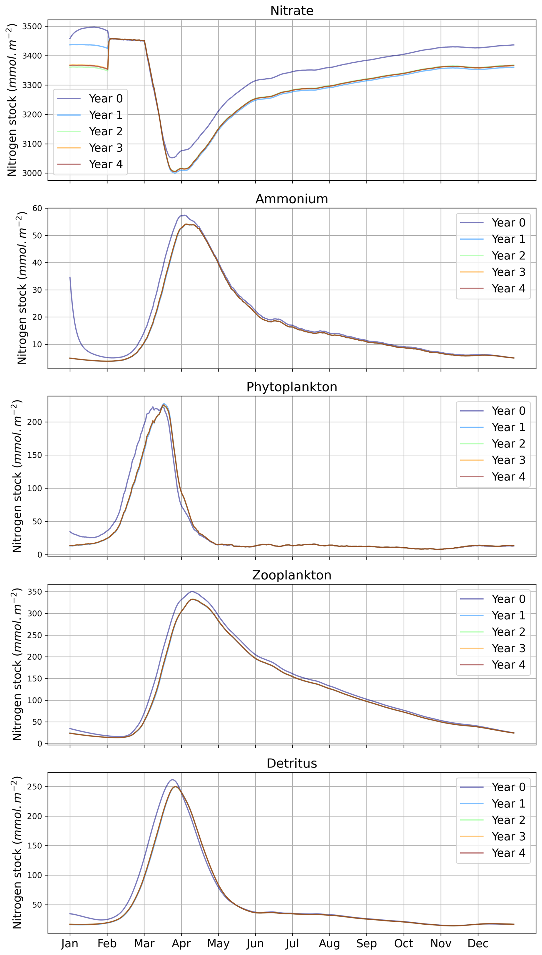
Figure C1 Simulated nitrogen stocks, averaged over one hundred samples across five consecutive years. The stocks are shown for nitrate, ammonium, phytoplankton, zooplankton, and detritus (from top to bottom). The one hundred samples constitute the test dataset and differ in their sets of BGC parameters and physical forcing.

Appendix D: Calibration under a configuration of perfect physics

Similarly to the experiment led in 0D in Littaye et al. (2025b), we conducted a calibration of parameters without physical forcing uncertainty. The evaluation metrics are presented in Fig. D1. A lower error mean and standard deviation for the BGC parameters was observed when using the 4Dvar scheme in comparison to the UNet. Furthermore, the simulated state components employing the estimated parameters demonstrate reduced correlation, elevated shift, and amplitude ratio values that deviate from one.

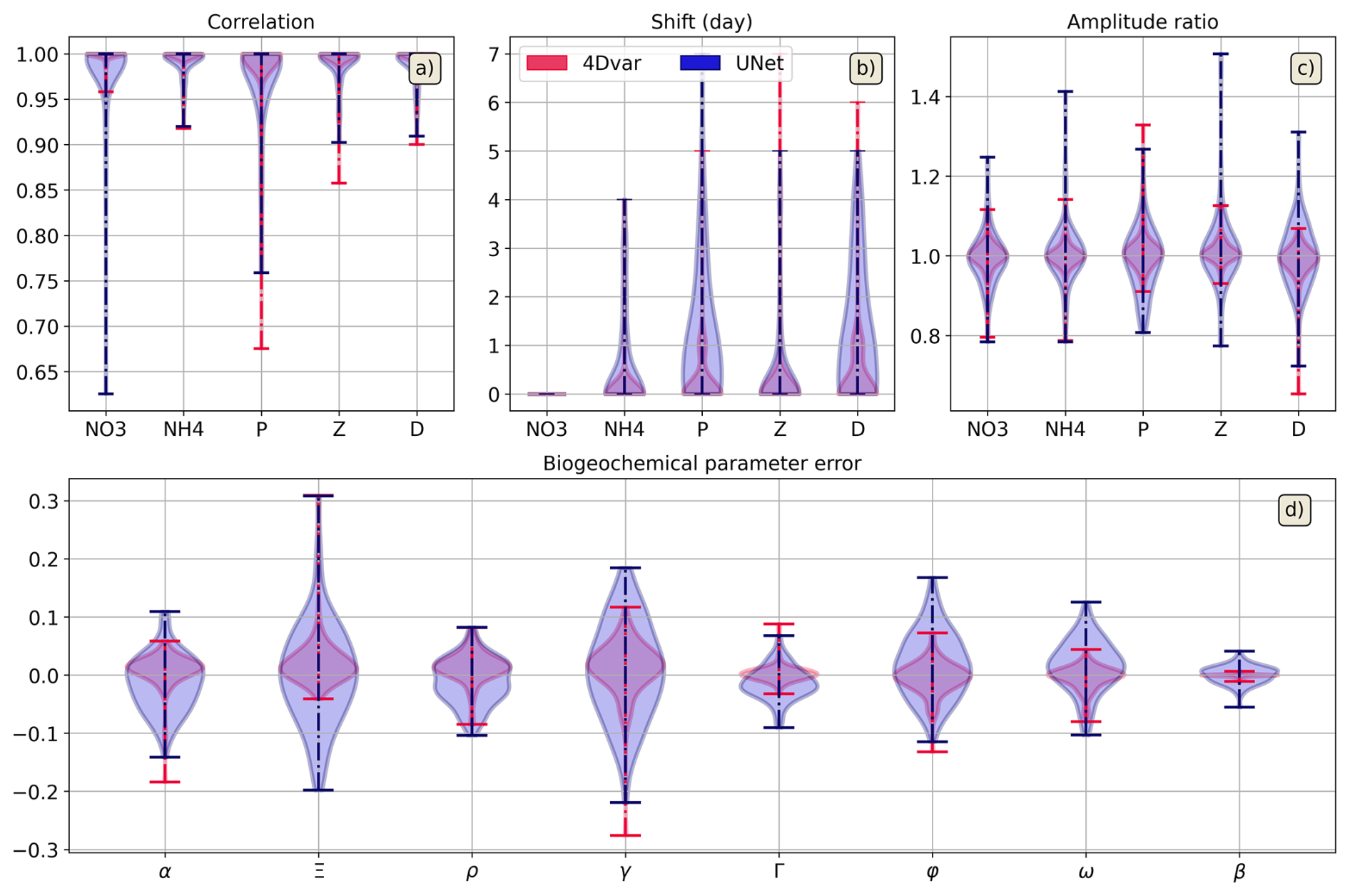
Figure D1 Evaluation metrics of the calibration of the BGC model. We assess a 4Dvar scheme (red distribution) and a learning-based scheme (blue distribution). We considered the following metrics: the correlation (a), the shift (b), the amplitude ratio (c) and the normalized parameter estimate error (d) as detailed in Sect. 3.5. We plot the distribution of the metrics for an evaluation dataset of 100 1D BGC simulations. We consider a scenario with no forcing uncertainty and a CTD + Rosette observation configuration with a 10 d sampling (Strategy 1 in Sect. 2.4).

Appendix E: Reanalysis of BGC dynamics with unobserved components

In Sect. 4.4, we compare three approaches – 4DVar, UNet, and the hybrid UNet + 4DVar – for refining BGC state variables. The hybrid configuration is initially assessed with a CTD + Rosette observation setup. Here, we report the same metrics (Table E1) and figure (Fig. E1) for an experiment in which ammonium and zooplankton are not observed (denoted as Strategy 2 – CTD in Sect. 2.4). Under this configuration, 4DVar performs poorly for the unobserved variables, with NMSE values of 1.6 and 1.3 for ammonium and zooplankton, respectively (see Table E1), while all other components exhibit NMSEs below 0.6. In contrast, UNet estimates all state variables with NMSEs not exceeding 0.1. The hybrid method yields only limited improvement over UNet in terms of accuracy, but it has the advantage of enforcing consistency with the governing model equations.

Figure E1 illustrates the estimated state variables for a representative ensemble member for each of the three approaches. The 4DVar estimates of ammonium and zooplankton are heavily biased, whereas the UNet produces estimates that are much closer to the reference solution. The hybrid scheme further smooths the estimated trajectories and ensures that they satisfy the BGC model dynamics.

Table E1 Table of the NMSE, standard deviation and representativeness of the reconstructed BGC states error, using Sampling Strategy 2 (see Sect. 2.4) for the three presented schemes: a 4Dvar-only-based scheme, a UNet-only-based scheme, and a hybrid scheme. The bold values refer to the lowest NMSEs and the highest “Distribution representativeness” within the three methods. The mean error is computed over the 10 members of the 100 samples for each BGC state. The standard deviation is computed from the 10-member ensemble of normalised reconstructed states and then averaged among the 100 samples. The representativeness of the data is indicated by the percentage of points of the true state that are comprised within the confidence interval of the distribution of the reconstructed state.

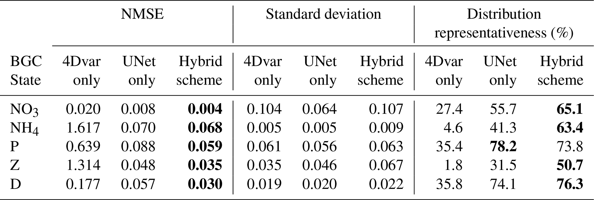
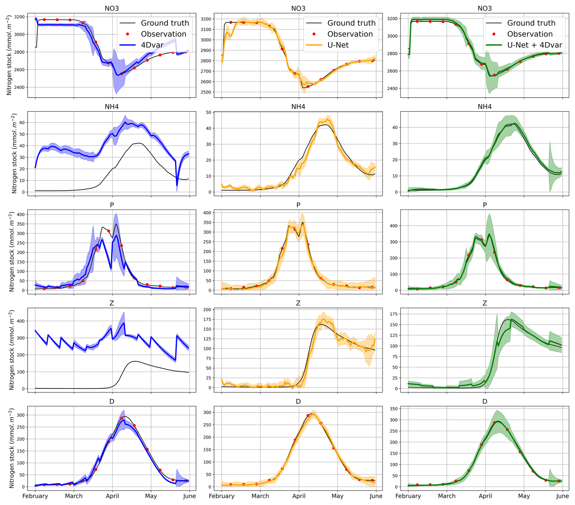
Figure E1 Reconstructed stocks associated with the five BGC states: NO₃, NH₄, P, Z and D; for one ensemble using a DA-based scheme (blue), a UNet-based scheme (orange) and a hybrid 4DVar + UNet base scheme (green), w.r.t. a scenario of case 1 forcing uncertainty, states observed with a 10 d time sampling and a CTD-only sampling strategy. The bold line indicates the mean stock among the 10-member ensemble, with the uncertainty, i.e., the mean value ±2σ with σ being the standard deviation of the ensemble. The aforementioned confidence interval is associated with the colourized shape. The ground truth is represented by the black curve. The observed states are denoted by red dots.

Appendix F: Refinement of BGC parameters and state components using a hybrid scheme

The hybrid strategy described in Sect. 3.4 is designed to improve the BGC state and parameters. The variables referred to as “refined” are in fact the optimised control variables. The results in Sect. 4.4 correspond to an experiment in which only the BGC components are refined. This choice stems from an initial experiment (see Fig. F1), which shows that it is not possible to refine the parameters and BGC components simultaneously. Using the hybrid method, the parameter NMSE reaches 0.41, compared with 0.12 for the UNet and 1.31 for the 4DVar scheme. Therefore, even though the physical forcings are corrected, the parameters estimated by the NN cannot be further refined with the hybrid approach.

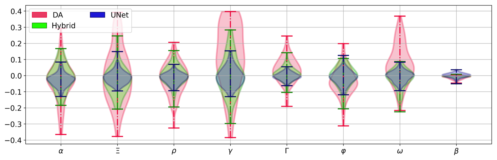
Figure F1 Evaluation metrics of the calibration of the BGC model. We assess a 4Dvar scheme (red distribution), a learning-based scheme (blue distribution) and a hybrid scheme (green distribution). We consider the normalized parameter estimate error as detailed in Sect. 3.5. We plot the distribution of the metrics for an evaluation dataset of 100 1D BGC simulations. We consider a baseline scenario given by low-level forcing uncertainties (case-1 scenario in Sect. 2.3) and a CTD + Rosette observation configuration with a 10 d sampling (Strategy 1 in Sect. 2.4).

Appendix G: Examples of BGC state sample reconstruction

Figure 11 presents a representative example of the mean performance of the DA, NN, and hybrid schemes in analysing BGC stocks. Figures G1 and G2 show two additional realisations from the same experiment. In Fig. G1, the BGC stocks produced by the hybrid scheme correspond to one of the highest scores reported in Table 2, whereas Fig. G2 illustrates a realisation associated with one of the lowest scores.

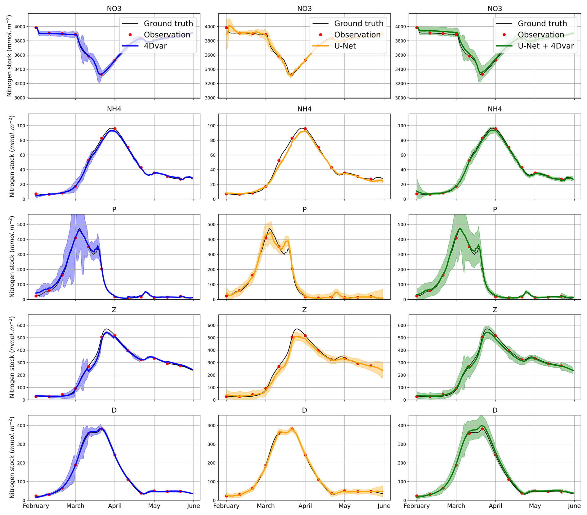
Figure G1 Plot of the reconstructed stocks associated to the five BGC states: NO₃, NH₄, P, Z and D; for one sample using a 4Dvar-based scheme (blue), a UNet-based scheme (orange) and a hybrid 4DVar + UNet base method (green), w.r.t. a scenario of case 1 forcing uncertainty, states observed with a 10 d time sampling and a CTD + Rosette-like sampling strategy. The bold line refers to the mean stock among the 10-members ensemble and the uncertainty, i.e., the mean value ±2σ with σ the standard deviation of the ensemble, is associated colourized shape. The ground truth is represented by the black curve.

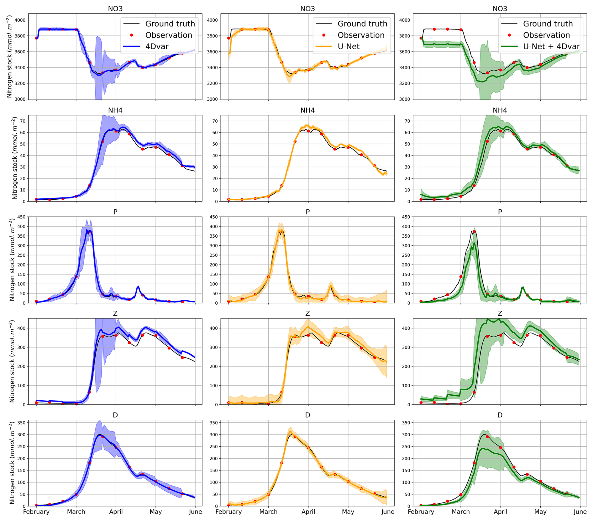
Figure G2 Plot of the reconstructed stocks associated to the five BGC states: NO₃, NH₄, P, Z and D; for one sample using a 4Dvar-based scheme (blue), a UNet-based scheme (orange) and a hybrid 4DVar + UNet base method (green), w.r.t. a scenario of case 1 forcing uncertainty, states observed with a 10 d time sampling and a CTD + Rosette-like sampling strategy. The bold line refers to the mean stock among the 10-members ensemble and the uncertainty, i.e., the mean value ±2σ with σ the standard deviation of the ensemble, is associated colourized shape. The ground truth is represented by the black curve.