What matters when? Temporal development of drivers and sources of nitrous oxide emissions in winter wheat

Agriculture is the largest anthropogenic source of nitrous oxide (N₂O), primarily due to nitrogen (N) fertilization. Understanding how the influence of key drivers and the relative contribution of source processes change throughout cropping seasons is crucial for developing effective strategies to mitigate N₂O emissions. In this study, we combined high-resolution eddy covariance (EC) flux measurements and explainable machine learning (ML) across the 2022–2023 winter wheat season and the subsequent summer cover crop at a temperate site in Switzerland, complemented by stable isotope analyses conducted in March 2023 following a fertilization event. We used Shapley Additive exPlanations (SHAP) to interpret an XGBoost model trained to predict N₂O fluxes, enabling a time-resolved assessment of driver contributions. Crop establishment and early spring emerged as particularly vulnerable periods, characterized by mismatches between N supply and plant demand that led to surplus soil mineral N and elevated N₂O fluxes under favorable moisture and temperature conditions. Elevated gross primary productivity (GPP, used as a proxy for crop activity and N demand) showed a consistent negative effect on N₂O fluxes, supporting the role of active vegetation as a competing N sink. Stable isotope source partitioning identified denitrification as the dominant N₂O production pathway during the early-spring post-fertilization period, consistent with poor soil drainage and high soil moisture. Cumulative N₂O emissions over the nine-month winter wheat season reached 5.5 kg N₂O-N ha⁻¹, with yield-scaled emissions of 1.1 kg N₂O-N Mg⁻¹ grain, both values exceeding those typically reported for wheat. Our findings highlight the value of combining EC, explainable ML, and stable isotope approaches to resolve the temporal dynamics of N₂O emissions and identify vulnerable windows for targeted mitigation in cropping systems.

1 Introduction

Nitrogen (N) is an essential nutrient for crop production, and the use of N fertilizers plays a central role in ensuring global food security (Erisman et al., 2008; Liang, 2022). However, a large part of the applied N is lost to the environment due to misalignment between the application (amount and timing) and crop demand (Ladha et al., 2005). Globally, only about 47 % of total fertilizer N input is taken up by crops, with most of the remainder lost through nitrate (NO${}_{\mathrm{3}}^{-}$) leaching, ammonia (NH₃) volatilization, contributing to water and air pollution, and through denitrification to nitrous oxide (N₂O) and dinitrogen (N₂) (Lassaletta et al., 2014; Scheer et al., 2020). Approximately 1 % of the applied N (IPCC, 2019) is emitted as N₂O, a potent greenhouse gas (GHG) with a 100-year global warming potential (GWP₁₀₀) of 273 times that of CO₂ (Forster et al., 2021), and the dominant ozone-depleting substance of the current century (Portmann et al., 2012; Ravishankara et al., 2009). Together with carbon dioxide (CO₂) and methane (CH₄), N₂O represents one of the three major GHGs contributing to anthropogenic climate forcing, with agricultural soils being a significant source of all three (Nabuurs et al., 2022). Despite accounting for a relatively minor fraction of N losses, the climate impact of N₂O makes its mitigation a key priority in sustainable agricultural management. Direct N₂O emissions from agricultural N additions are the largest source of anthropogenic N₂O emissions, accounting for 56 % of global emissions over the past decade (Tian et al., 2024), with more than half (55 %) originating from soils following fertilizer application. The remaining fraction is attributed to manure excreted on pastures and manure management (Epper et al., 2025; Tian et al., 2024). In Switzerland, N₂O emissions account for approximately 30 % of total agricultural GHG emissions (FOEN, 2026). At both EU and Swiss levels, policies have been introduced to reduce N losses from agriculture and mitigate associated environmental impacts, such as the EU Nitrates Directive (European Commission, 1991) and Switzerland's Water Protection Ordinance (Swiss Federal Council, 1998). However, despite the well-documented climate effects of N₂O, binding measures specifically targeting N₂O mitigation are still lacking (Epper et al., 2025). This regulatory gap hinders the development and implementation of effective mitigation strategies, leaving a major source of agricultural GHG emissions largely unaddressed.

N₂O in soils is primarily produced through microbial nitrification and denitrification (Butterbach-Bahl et al., 2013). Several interacting factors, including N substrate availability (i.e., NH${}_{\mathrm{4}}^{+}$ and NO${}_{\mathrm{3}}^{-}$), soil moisture, temperature, pH, and labile carbon supply, affect both production of N₂O and reduction of N₂O to N₂, the final product of denitrification (Davidson, 1991; Rummel et al., 2025; Saggar et al., 2013; Smith, 2017). Agronomic operations such as fertilization and tillage increase N availability and stimulate microbial N₂O production (Chatskikh and Olesen, 2007; Shcherbak et al., 2014). Recent studies also highlight the role of actively growing vegetation as a dynamic N sink that competes with microbes for N substrates, thereby reducing their availability for N₂O production and mitigating N₂O emissions (Abalos et al., 2018; Feigenwinter et al., 2023; Maier et al., 2022; Timilsina et al., 2024). Accordingly, the N surplus, defined as the difference between total N inputs and outputs, correlates positively with N₂O emissions (Tallec et al., 2022; Van Groenigen et al., 2010). However, the spatio-temporal heterogeneity of environmental and management-related drivers, along with the high temporal variability of N₂O fluxes, pose major challenges for identifying key drivers of N₂O emissions throughout the cropping season. Across the cropping cycle, from field preparation to post-harvest, N₂O emissions are shaped by changes in soil environmental conditions, N availability, and management (Smith et al., 1998; Garnier et al., 2024). While many studies have explored the general relationships between individual drivers and N₂O emissions, to our knowledge, no study has systematically investigated how the relative importance of these drivers changes over the course of a cropping season. Therefore, our understanding of these temporal dynamics is still scarce, limiting the development of mitigation strategies because these may only be effective when aligned with the dominant emission controls at specific stages of the cropping season.

In addition to N₂O, croplands exchange substantial amounts of CO₂ and CH₄ with the atmosphere, which together determine their net GHG budget (Carlson et al., 2017; Ciais et al., 2010; Schulze et al., 2009). CO₂ fluxes reflect the difference between photosynthetic CO₂ uptake and ecosystem respiration, whereas CH₄ fluxes from agricultural soils result from concurrent microbial production (i.e., methanogenesis) and oxidation (i.e., methanotrophy) (Le Mer and Roger, 2001). Quantifying these fluxes alongside N₂O is crucial for an integrated assessment of the cropland GHG budget and its response to environmental and management drivers.

To improve our understanding of the temporal dynamics of N₂O emissions and their contribution to the net GHG budget, continuous and spatially integrated measurements of N₂O fluxes are essential. Micrometeorological techniques such as eddy covariance (EC) enable continuous, high-frequency observations of N₂O fluxes, spatially integrating over entire fields (Feigenwinter et al., 2023; Lognoul et al., 2019; Maier et al., 2022, 2025). When EC-based N₂O flux measurements are combined with concurrent observations of key environmental and management-related drivers, they can provide valuable insights into the temporal dynamics of N₂O emissions and their controls throughout the cropping season. Building on high-resolution data provided by EC systems, machine learning (ML) algorithms offer powerful tools to model N₂O emissions (Gnisia et al., 2025; Goodrich et al., 2021; Hamrani et al., 2020). These ML models can capture non-linear relationships and complex interactions among environmental and management-related drivers and often outperform traditional statistical approaches in predictive accuracy (Philibert et al., 2013; Saha et al., 2021). Furthermore, model explanation techniques such as SHapley Additive exPlanations (SHAP; Lundberg and Lee, 2017) enhance the interpretability of ML models by quantifying the contribution of individual drivers, offering insights into the temporal evolution of driver importance (Krebs et al., 2025; Scapucci et al., 2024, 2025).

While ML models can identify which environmental and management variables most influence N₂O fluxes, they do not reveal the underlying microbial production processes. Recent work has shown that modelling distinct N₂O emission regimes may help infer dominant production pathways (Lussich et al., 2026), but such attribution remains indirect. Nevertheless, such attribution is important because nitrification and denitrification respond differently to environmental conditions (Butterbach-Bahl et al., 2013; Davidson, 1991) and management (Buchen et al., 2018). Distinguishing between these two sources of N₂O is essential for developing targeted mitigation strategies and improving the accuracy of process-based biogeochemical models (Del Grosso et al., 2020). Stable isotope analysis, particularly of the intramolecular distribution of ¹⁵N (i.e., the so-called site preference, SP), is an established approach to identify the relative contributions of nitrification and denitrification to N₂O production (Pérez et al., 2001). Both processes generate N₂O with distinct isotopic signatures due to differences in enzymatic mechanisms and substrate pools. Because SP is largely independent of the isotopic composition of precursor substrates, it contributes to the partitioning of N₂O sources under field conditions (Decock and Six, 2013). Combined with nitrogen and oxygen stable isotope ratios (δ¹⁵N and δ¹⁸O, respectively), SP can be used to trace the temporal development of N₂O-producing processes and constrain the extent of N₂O reduction to N₂(Verhoeven et al., 2019; Yu et al., 2020).

The present study integrates continuous EC measurements and ML-based driver analysis over a winter wheat cropping season and the following short summer cover crop at a temperate European site, complemented by stable isotope measurements during a sampling campaign in spring. Specifically, we aimed to (i) quantify N₂O, CO_2, and CH₄ fluxes and resulting GHG budgets throughout a winter wheat cropping season and the subsequent cover crop season, (ii) determine the temporal development of environmental and management driver contributions to N₂O fluxes, and (iii) identify the contributions of different microbial N₂O-producing processes and their temporal development during the weeks following a fertilization event.

2 Material and methods

2.1 Study site

The study site is a cropland field in Oensingen, canton of Solothurn, Switzerland. The site has a mean annual temperature of 10.1 °C and receives an average of 1151 mm of precipitation per year (2004–2023). CO₂ and water vapor (H₂O) fluxes have been continuously measured at the site by an EC station (CH-Oe2, part of FLUXNET and Swiss FluxNet; 47°1^′11.1^′′ N, 7°44^′01.5^′′ E; 452 m a.s.l.) since December 2003 (Emmel et al., 2018). The field where the station is positioned has an area of 1.55 ha, and the soil is classified as Eutric-Stagnic Cambisol with a silty clay texture. In the top 0.25 m, the soil consists of 43 % clay, 47 % silt, and 10 % sand, with 2.8 % organic matter (Alaoui and Goetz, 2008). In the top 0.1 m depth, soil pH is 6.4 (Maier et al., 2025), and bulk density is 1.27 g cm⁻³. Carbon and nitrogen stocks in the 0–0.7 m soil profile, derived from Emmel et al. (2018), are 18.6 kg C m⁻² and 1.9 kg N m⁻², respectively. The field is managed according to an integrated farming label (IP Suisse) and follows the Proof of Ecological Performance (PEP; Swiss Federal Council, 2025). PEP sets baseline requirements for receiving direct payments, including rules for crop rotation, farm-based fertilizer use, and measures to protect soil and biodiversity. Over the past 20 years, the crop rotation included various annual crops, with winter wheat as primary crop. A temporary grassland (grass-clover mixture; STEFFEN 3003M, Samen STEFFEN AG) was established in 2020 and managed until its final cut in late September 2022, followed by herbicide application (Glyphosate) and direct-seeding of winter wheat. This study was conducted over one year, from September 2022 to October 2023, covering the last month of the temporary grassland, the full winter wheat growing season, and the subsequent cover crop season, a mixture of legumes, grasses, and forbs (Terra-FIT Quattro, Samen STEFFEN AG). Winter wheat (Montalbano, bred by Agroscope and DSP) was sown on 6 October 2022, and harvested on 15 July 2023, with 5.03 t ha⁻¹ grain yield (dry matter). The winter wheat received three applications of mineral and organic (dairy slurry) fertilizers between late tillering and early stem elongation, summing up to 138 kg N ha⁻¹ (Table 1). After the harvest, the straw was removed from the field, and the soil was cultivated for the subsequent sowing of the summer cover crop. The cover crop was mulched in late September 2023, before the soil was cultivated again to prepare for the sowing of winter barley in early October 2023.

Table 1 Main management activities conducted during the 2022–2023 measurement period at the cropland in Oensingen. Positive values for nitrogen (N) input/output indicate inputs to the field, whereas negative values represent N exports. For the slurry application, total N is reported, which included 18 kg NH${}_{\mathrm{4}}^{+}$-N ha⁻¹. Due to a sampling issue in 2023, slurry composition was estimated based on laboratory analysis of a 2024 sample from the same farm. Details on commercial products and additional management practices are provided in Table A1.

2.2 Eddy covariance flux measurements

2.2.1 Setup

The EC setup, situated at the center of the field, consisted of an ultrasonic anemometer (R3-50, Gill Instruments Ltd., Lymington, UK) that measured wind speed, and a laser spectrometer that measured N₂O and CH₄ concentrations at 10 Hz (GLA351-N2OM1, Los Gatos Research, Mountain View, CA, USA), as well as an enclosed infrared gas analyzer (IRGA) that measured CO₂ and H₂O concentrations at 20 Hz (LI-7200, LI-COR Biosciences, Lincoln NE, USA). The laser spectrometer was connected to an external pump (EV-A06, Ebara Technologies, Sacramento, CA, USA) and both were placed in temperature-controlled boxes. A 7 m long, 7.5 mm diameter unheated polyethylene/aluminum composite tube (EATON Synflex 1300, Dublin, Ireland) was used to draw air to the laser spectrometer. The measurement height of the sonic anemometer was 2.17 m above ground, and the inlets of the laser spectrometer and the IRGA were mounted approximately 0.2 m below the sonic anemometer. While CO₂ and H₂O fluxes have been measured continuously since 2003, N₂O and CH₄ flux measurements were conducted during selected periods between 2018 and 2021 (Maier et al., 2025), followed by continuous measurements from 30 August 2022 to 5 October 2023 in the present study.

2.2.2 Flux processing

Half-hourly fluxes of CO₂, H₂O (i.e., as latent heat flux (LE)), as well as N₂O and CH₄fluxes were calculated using the EddyPro software (version 7.0.9, LI-COR Environmental, Lincoln NE, USA) following established EC flux community protocols (Aubinet et al., 2012; Nemitz et al., 2018; Pastorello et al., 2020; Sabbatini et al., 2018). Raw high-frequency data underwent de-spiking and screening, in line with Vickers and Mahrt (1997), and wind components were aligned using a 2D rotation method (Wilczak et al., 2001). The time lag between the vertical wind component and scalar concentration of N₂O and CH₄ was set to a constant value, corresponding to the most frequently occurring lag (1.40 s for N₂O and 1.50 s for CH₄) identified through covariance maximization within a broad window (0–5 s) over the entire measurement period. In contrast, time lags for CO₂ and LE were determined dynamically through covariance maximization within narrow windows, based on prior lag distributions identified using a broader window. When no clear covariance peak was detected within the defined window, a default lag was applied (1.30 s for CO₂, 1.45 s for H₂O), corresponding to the most frequently identified lag in the earlier analysis. Spectral corrections addressed high-pass (Moncrieff et al., 2005) and low-pass filtering effects (Fratini et al., 2012). A correction for instrument separation was applied (Horst and Lenschow, 2009). The flux footprint model by Kljun et al. (2015) estimated the upwind area contributing to the measured flux.

2.2.3 Quality assessment and de-spiking

Data quality was assessed using a composite flag (QC0 = best quality, QC1 = medium quality, QC2 = bad quality), calculated with the Python library diive (v0.86.0; Hörtnagl, 2025). The flag included tests for (1) steady-state and integral turbulence characteristics (Mauder and Foken, 2004), (2) spectral correction factor (values with spectral correction factor > 4 were excluded), (3) IRGA signal strength, (4) completeness of the averaging interval (if < 97 % coverage within 30 min, value was excluded; Sabbatini et al., 2018), and (5) occurrence of spikes and drop-outs in the raw data after the statistical tests by Vickers and Mahrt (1997). Fluxes with the quality flag 2 (QC2) were excluded from further analyses. Storage terms (single point measurement) were added to all measured gas fluxes (Aubinet et al., 2001). CO₂ fluxes are referred to as net ecosystem exchange of CO₂ (NEE) from this point onwards. Absolute limits were applied to remove half-hourly fluxes outside plausible ranges, determined by analysing typical ranges for highest-quality fluxes (NEE: −60 to 50 µmol m⁻² s⁻¹; LE: −50 to 800 W m⁻²; N₂O flux: −3 to 30 nmol m⁻² s⁻¹; CH₄flux: −30 to 80 nmol m⁻² s⁻¹). Outliers were further removed by sequentially applying one or more of the following filters, as needed: rolling standard deviation, Hampel, and rolling Z-score, as these methods capture different types of anomalies. Finally, a friction velocity (u_*) filter (Papale et al., 2006) was applied to NEE, N₂O, and CH₄ fluxes to exclude periods with insufficient turbulence conditions. The threshold was determined using CO₂ fluxes, and a constant u_* threshold of 0.092 m s⁻¹ was used for the entire study period. After applying all quality checks, de-spiking, and u_* filtering, data coverage for fluxes over the entire measurement period was 50.8 % for NEE, 68.5 % for LE, 52.9 % for N₂O flux, and 33.6 % for CH₄ flux. Gaps were predominantly short (median: two records for NEE and CH₄, one record for N₂O), with >99.6 % lasting < 1 d. Only one gap for NEE and five gaps for N₂O and CH₄ exceeded three days, and only one gap for N₂O and CH₄ exceeded seven days (none for NEE); maximum gap lengths were ∼ 5 d for NEE and ∼ 9 d for N₂O and CH₄ (Table A2). Only the highest quality N₂O fluxes (QC0, 34.5 % data coverage) were used for the driver analysis. Further details on data quality control procedures and outlier removal methods are available in the project repository (Turco, 2025). Flux rates are reported as µmol CO₂ m⁻² s⁻¹ for NEE, nmol N₂O m⁻² s⁻¹ for N₂O flux, and nmol CH₄ m⁻² s⁻¹ for CH₄ flux, while cumulative fluxes are reported as g C m⁻² (NEE, CH₄) or kg N₂O-N ha⁻¹ (N₂O).

2.2.4 Gap-filling and NEE partitioning

Gap-filling of N₂O and CH₄ fluxes was performed using a Random Forest (RF) regressor (Breiman, 2001) as implemented via the diive Python library (v. 0.86.0), based on the scikit-learn framework. Although a systematic comparison of gap-filling methods for eddy covariance N₂O fluxes is still lacking, RF has been shown to outperform conventional approaches for CH₄ fluxes (Irvin et al., 2021; Kim et al., 2020), supporting its use here for both non-CO₂ gases. Predictor (i.e., driver) variables were selected based on their demonstrated predictive performance in previous studies (Feigenwinter et al., 2023), including environmental data (and their lagged variants), management information (expressed as time since event), and timestamp features. Environmental variables comprised soil temperature, precipitation (in absolute terms and time since occurrence), and soil water content. For model training and evaluation, each dataset was randomly split into training and test subsets, with 25 % of the data reserved for testing. Model performance differed markedly between gases. For N₂O fluxes, the model achieved an R² of 0.79, with a MAE of 0.40 and a RMSE nmol m⁻² s⁻¹ of 0.90. In contrast, performance for CH₄ fluxes was poor, with an R² of −0.05, a MAE of 5.8 nmol m⁻² s⁻¹, and a RMSE of 8.7 nmol m⁻² s⁻¹. Although we did not systematically assess gap-filling uncertainty as a function of gap length (Bigaignon et al., 2020; Taki et al., 2019), this limitation is partly mitigated by the generally short gap lengths in our dataset (Table A2).

For NEE and LE, gap-filling was conducted using the Marginal Distribution Sampling (MDS) method (Reichstein et al., 2005), implemented in R via the REddyProc package (v. 1.3.2; Wutzler et al., 2018). Input variables for MDS included global radiation, air temperature, and vapor pressure deficit. NEE was subsequently partitioned into gross primary production (GPP) and ecosystem respiration (R_eco) using the night-time method (Reichstein et al., 2005), also implemented in REddyProc (Wutzler et al., 2018). Additional methodological details and code are available in the project repository (Turco, 2025).

2.3 Calculation of net GHG exchange and net GHG budget

Cumulative N₂O, CH₄, and CO₂ fluxes were calculated separately for the winter wheat cropping season and the subsequent cover crop period using gap-filled flux datasets. The winter wheat cropping season was defined as the period from sowing to harvest, while the cover crop period was defined as the period from cover crop sowing to mulching. To express fluxes in terms of CO₂-equivalents, global warming potential (GWP₁₀₀) values of 273 for N₂O and 27 for CH₄ were applied, in accordance with current estimates (Forster et al., 2021). The sum of N₂O, CH₄ and CO₂, i.e., the cumulative fluxes expressed in CO₂-equivalents (CO₂-eq), is hereafter referred to as net GHG exchange (NGHGE). This term is used to distinguish the EC-based atmospheric exchange from the net GHG budget, which additionally accounts for lateral C imports and exports.

The net GHG budget was derived from the C budget, which combines NEE with lateral C fluxes from management (imports and exports). C exports comprised harvested grain and straw, and C imports comprised organic fertilizer additions. Exports were treated as positive fluxes (C removal from the ecosystem) and imports as negative fluxes (C addition). The C budget was converted to CO₂-eq using the molecular mass ratio of CO₂ to C, then N₂O and CH₄ fluxes (in g CO₂-eq) were added to obtain the net GHG budget, following Ammann et al. (2020). Negative values indicate a net GHG sink, positive values a net GHG source.

To assess the sensitivity of NGHGE to friction velocity (u_*) filtering (Table A3), cumulative N₂O, CH₄ and CO₂ fluxes and the resulting NGHGE were calculated under alternative u_* thresholds, corresponding to the 16th and 84th percentiles of the bootstrapped u_* threshold distribution (CUT16 and CUT84, respectively), in addition to the default threshold (CUT50; median), following Pastorello et al. (2020).

The N₂O emission factor (EF) for the winter wheat season was calculated by dividing the cumulative N₂O-N emissions from sowing to harvest by the total amount of N from mineral and organic fertilizers. The resulting EF is expressed as the percentage of the applied N that is emitted as N₂O-N. Because no unfertilized control treatment was available, non-fertilization-induced emissions could not be subtracted. The resulting value, therefore, represents an apparent EF rather than an IPCC Tier 1 EF. To account for N₂O emissions beyond the winter wheat season, we additionally calculated an annual apparent EF for the one-year period starting at winter wheat sowing, including the bare-soil period after harvest and the subsequent cover crop period. This metric was calculated as cumulative annual N₂O-N emissions divided by the fertilizer N applied during the same period.

2.4 Meteorological and soil variables

The meteorological variables air temperature and relative humidity (CS215, Campbell Scientific Ltd., Logan UT, USA), atmospheric pressure (PAA-33X, Keller AG, Switzerland), short- and longwave radiation (CNR4, Kipp & Zonen, Delft, Netherlands), photosynthetic photon flux density PPFD (BF5, Delta-T Devices, United Kingdom), and precipitation (heated tipping bucket rain gauge, Lambrecht meteo GmbH, Germany) were measured continuously at the EC station. Soil water content and soil temperature were also measured continuously close to the EC station along one soil profile (at 0.05, 0.15, 0.3, and 0.5 m soil depths) using 5TM sensors (Decagon Devices, Inc., Pullman WA, USA). All meteorological measurements were recorded at one-minute time resolution and, after screening for outliers, averaged to 30 min values (precipitation was summed). Water-filled pore space (WFPS; Eq. 1) was calculated for each soil depth as:

$$\begin{array}{}\text{(1)}& \mathrm{WFPS}={\displaystyle \frac{\mathrm{SWC}}{\mathrm{1}-\frac{\mathrm{BD}}{\mathrm{PD}}}}\cdot \mathrm{100}\end{array}$$

where SWC is the volumetric soil water content (in m³ m⁻³), BD is the bulk density (in g cm⁻³), with values of 1.16, 1.40, and 1.33 g cm⁻³ for the 0–0.05, 0.15–0.3, and 0.3–0.5 m depth intervals, respectively, obtained from Emmel et al. (2018), and PD is the particle density, assumed to be 2.65 g cm⁻³ (Danielson and Sutherland, 1986). Because SWC was measured at a single soil profile, absolute WFPS estimates may not fully represent spatial variability across the EC footprint. However, similar SWC dynamics observed at an independent sensor profile located a few meters away indicated that temporal patterns were representative. The WFPS conversion further relied on bulk density values from Emmel et al. (2018), which may not fully reflect topsoil conditions during this experiment. Therefore, uncertainty is expected mainly in absolute WFPS values rather than in temporal WFPS dynamics.

2.5 Soil chamber measurements and stable isotope analyses

Five opaque static PVC (polyvinyl chloride) chambers, each with a volume of 17.7 L and a surface area of 0.07 m², were deployed at five randomly selected locations within a 12 m radius of the EC station (Fig. 1). The chambers were first deployed on 24 February 2023, before the first fertilization event, and positioned to enclose plants from two adjacent wheat rows. To ensure that regular field management could continue unhindered, the chambers were removed immediately after sampling when management operations were scheduled before the next sampling date and subsequently reinstalled at the same positions for the following measurements. In total, six sampling campaigns were conducted between 24 February and 17 March 2023, encompassing the period around the first fertilizations (27 and 28 February) and two campaigns later in the season (31 May and 19 July). The sampling was performed around midday (typically between 11:00 and 13:00 local time) to minimize diurnal variability in fluxes. For each chamber and time point, two headspace samples were collected: one immediately after chamber closure (t₀), and one after a 1-hour enclosure period (t₆₀). Air samples were drawn from the chamber headspace with a 60 mL syringe. For subsequent N₂O concentration analysis, 20 mL of the air sample was injected into pre-evacuated 12 mL vials. For stable isotope analyses, 180 mL of the air sample was injected into pre-evacuated 110 mL serum crimp vials. During each sampling campaign, a soil sample was collected for each chamber by combining two soil cores (0–0.1 m depth) taken approximately 0.3 m from the chamber edge. The pooled samples were placed into Schott tubes, which were immediately sealed with Parafilm, enclosed in plastic bags, and stored in a cooling box before being transferred to a freezer at −18 °C. Soil water was later extracted from the samples using cryogenic vacuum distillation (Ehleringer and Osmond, 2000). The stable oxygen isotope ratio (δ¹⁸O) of the extracted water was then measured using an isotope ratio mass spectrometer (IRMS; DeltaplusXP, Finnigan MAT, Bremen, Germany) and expressed in the delta notation referenced to the Vienna Standard Mean Ocean Water (V-SMOW) in ‰ (Eq. 2) as:

$$\begin{array}{}\text{(2)}& {\mathit{\delta }}^{\mathrm{18}}\mathrm{O}={\displaystyle \frac{R_{\mathrm{sample}}}{R_{\mathrm{reference}}}}-\mathrm{1}\end{array}$$

where R denotes the ratio of ¹⁸O $/$ ¹⁶O.

N₂O gas samples were analyzed for their stable N and oxygen isotope ratios (δ¹⁵N^bulk, δ¹⁸O, respectively) as well as the site preference (SP-N₂O) using a trace gas preparation unit (Elementar, Manchester, UK) coupled to an IsoPrime100 IRMS (Elementar, Manchester, UK). Calibration and data correction followed the procedure described in Verhoeven et al. (2019) and in Gallarotti et al. (2021), including the use of multiple working standards and correction for instrumental drift, span, and linearity. In addition, instrument performance was regularly assessed using standards treated as samples (Werner and Brand, 2001), ensuring data quality and interlaboratory comparability (Mohn et al., 2014). Site preference (SP) represents the difference between the N isotope ratios at the central (α) and terminal (β) N positions of the N₂O molecule. Unlike δ¹⁵N^bulk, SP-N₂O is independent of the initial substrate, making it a more direct indicator of the N₂O production pathway (Toyoda et al., 2002). The isotopic signature of emitted N₂O was calculated using the following two-point mixing equation (Eq. 3):

$$\begin{array}{}\text{(3)}& {\mathit{\delta }}^Z\mathrm{X}={\displaystyle \frac{{\left[{\mathrm{N}}_{\mathrm{2}}\mathrm{O}\right]}_{\mathrm{e}}\cdot {\mathit{\delta }}^Z{\mathrm{X}}_{\mathrm{e}}-{\left[{\mathrm{N}}_{\mathrm{2}}\mathrm{O}\right]}_{\mathrm{s}}\cdot {\mathit{\delta }}^Z{\mathrm{X}}_{\mathrm{s}}}{{\left[{\mathrm{N}}_{\mathrm{2}}\mathrm{O}\right]}_{\mathrm{e}}-{\left[{\mathrm{N}}_{\mathrm{2}}\mathrm{O}\right]}_{\mathrm{s}}}}\end{array}$$

where [N₂O]_s and [N₂O]_e are the N₂O mixing ratios [ppb] at t₀ and t₆₀, respectively, measured using a gas chromatograph equipped with an electron capture detector (456-GC, Scion Instruments, Livingston, WLO, UK), while δ^ZX_s and δ^ZX_e are the corresponding isotope ratios (‰). A threshold of 30 ppb in N₂O concentration increase (Δ[N₂O] = [N₂O]_e − [N₂O]_s) was used to exclude flux estimates for which the change in N₂O concentration during the chamber closure was too small to yield reliable isotopic signatures (Harris et al., 2020b). N₂O fluxes on four of the eight sampling dates, 1, 3, 6, and 17 March, exceeded this threshold and were subsequently included in the analyses. Thus, isotope-based process identification was restricted to the three weeks following the first fertilization events at the end of February 2023 (Table A1).

To determine the main production pathways of N₂O, a dual isotope mapping approach was used, relating (i) δ¹⁸O-N₂O to SP-N₂O, and (ii) δ¹⁵N^bulk-N₂O to SP-N₂O. The mixing endmembers for nitrification (Ni), heterotrophic bacterial denitrification (bD), nitrifier denitrification (nD), and fungal denitrification (fD) were chosen according to Yu et al. (2020). The δ¹⁸O-N₂O endmembers of bD, nD, and fD were adjusted by the mean δ¹⁸O of soil water to account for the oxygen isotopic signature of the substrate (Lewicka-Szczebak et al., 2020). Since no measurements of the δ¹⁵N of soil N precursors were available, a δ¹⁵N value of 0 ‰ was assumed for precursor nitrate and ammonium in the δ¹⁵N^bulk-N₂O vs. SP-N₂O map. The contributions of different N₂O production pathways and the residual fraction of unreduced N₂O (r) were estimated with the FRAME software, implementing a Markov Chain Monte Carlo model (Lewicki et al., 2022). The FRAME model was configured using process-specific mean values and fractionation factors from Yu et al. (2020), and the δ¹⁸O-N₂O mean values were corrected for δ¹⁸O-H₂O. For each sample, the uncertainty of the isotopic signature of the emitted N₂O was obtained by Gaussian error propagation through Eq. (3), from the uncertainties of the four measured input quantities (δ^ZX and [N₂O] at t₀ and t₆₀). As no replicate samples were available, conservative analytical precisions of 1 ‰ (1 SD) for the isotopic measurements and 2 % (1 SD, relative) for the N₂O concentrations were assumed. This assumed uncertainty for the isotopic measurements is larger than the analytical uncertainties typically reported for IRMS-based N₂O isotopocule analysis (Mohn et al., 2014). The resulting sample-specific uncertainties were then used as the measurement uncertainties in FRAME and are therefore reflected in the posterior distributions. FRAME was run using the mixing-reduction scenario, in which N₂O from different production pathways is mixed before partial reduction to N₂. Instead of the residual unreduced N₂O fraction (r), we report the reduced fraction (1−r), as it is more intuitive to interpret. To test sensitivity to the assumed order of mixing and reduction, the alternative reduction-mixing scenario was also tested, in which denitrification-derived N₂O is reduced before mixing with N₂O from the other pathways.

2.6 Vegetation and soil measurements

Leaf area index (LAI), vegetation height, and phenological development stages were monitored throughout the study. From March to July 2023, measurements were conducted at 2- to 3-week intervals to capture the growth dynamics during the most active vegetative period of winter wheat, and at key developmental stages before and after this period. LAI and canopy height were measured at six locations spread 5 m apart along four transects originating from the EC station (Fig. 1). LAI was measured using a LAI-2000 Plant Canopy Analyzer (LI-COR Biosciences, USA) by taking one above-canopy and six below-canopy readings for each transect. Under clear sky conditions, measurements were conducted towards the north to avoid direct sunlight on the lens. Vegetation height was determined by measuring the height of an expanded polystyrene plate of 0.25 m² dropped on top of the vegetation at each spot (Ammann et al., 2007). Phenological development stages of winter wheat were identified according to the BBCH-scale (Meier, 2018) for five plants randomly selected in the field.

Aboveground biomass (AGB) was sampled monthly, using a harvest frame with a defined area of 0.1 m². Three samples were randomly collected at each of the four defined field sections (Fig. 1), and entire wheat plants were cut 2 cm above the ground. At harvest, grain and straw were sampled separately to estimate C and N exports from the field. The dry weight was determined after drying all plant samples at 60 °C for 48 h. The dried samples were further processed by first cutting the biomass into smaller pieces, then a subsample was ground to a fine powder with a ball mill (MM200, Retsch, Germany). Finally, about 4 mg was weighed into small tin capsules, and carbon (C) and N concentrations (in %) were determined with a Flash EA 1112 elemental analyzer (Thermo Italy, former CE Instruments, Rhodano, Italy).

Soil mineral N was measured during the wheat cropping season to quantify the instantaneous extractable inorganic N pools. Soil samples were collected five times using a machine-assisted soil core sampler within the same field sections used for AGB sampling, with ten to fifteen soil cores taken at each section and bulked for each soil depth (0–0.3, 0.3–0.6, and 0.6–0.9 m). Ammonium (NH${}_{\mathrm{4}}^{+}$) and nitrate (NO${}_{\mathrm{3}}^{-}$) were extracted by an external laboratory using a 0.01 M CaCl₂ solution at a 1:4 soil-to-solution ratio, following the Swiss reference method (Buerge, 2020) established by the Federal Agriculture Research Center, Agroscope. Concentrations were photometrically determined by the same laboratory and reported in mg N per 100 g of dry soil. Soil mineral N (N_min) was then calculated in kg N ha⁻¹ using the same reference method.

Plant Root Simulator probes (PRS™, Western Ag, Saskatoon, Canada) were used as a complementary measure of plant-available N supply over time. In contrast to N_min measurements, which provide a snapshot of extractable inorganic N at the time of sampling, PRS probes integrate ion supply to exchange membranes over the burial period and therefore provide a time-integrated estimate of available N supply. Measurements of plant-available soil N complemented soil sampling from March to September 2023. Three PRS sets, each consisting of one anion and one cation exchange resin probe (17.5 cm² surface area each), were buried at 0–0.1 m soil depth. This depth was chosen to target the soil layer most strongly affected by management and where root density and nutrient uptake are highest. The probes were positioned along the wheat inter-row at the same five locations used for chamber measurements (Fig. 1). The probes were replaced every two to three weeks, resulting in seven burial periods. No probes were buried in June due to technical issues, nor in the second half of July due to tillage and sowing operations. Prior to shipment to Western Ag for analyses, the PRS probes were rinsed with deionized water and stored at 5 °C. Extraction of NH${}_{\mathrm{4}}^{+}$ and NO${}_{\mathrm{3}}^{-}$ with 0.5 mol L⁻¹ HCl was conducted by pooling all three PRS sets from each location, yielding one value per location and sampling period (in µg N per 10 cm² per time of burial). Since all NH${}_{\mathrm{4}}^{+}$ measurements were below the detection limit (except for one sample), we excluded NH${}_{\mathrm{4}}^{+}$-N from further analyses.

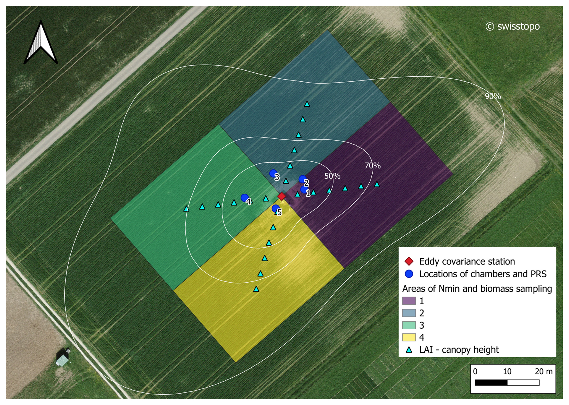
Figure 1 Experimental setup at the study site in Oensingen during the 2022–2023 measurement period. The red diamond marks the eddy covariance station; white lines delineate the 50 %, 70 %, and 90 % average footprint areas (based on the Kljun et al., 2015 model); blue dots indicate locations of manual chambers and plant root simulator (PRS) probes; colored rectangles show areas for Nmin and aboveground biomass sampling; triangles denote fixed locations for LAI and canopy height measurements. Orthophoto: © Federal Office of Topography swisstopo.

2.7 Investigating the temporal development of N₂O drivers

2.7.1 XGBoost model

To investigate biotic and abiotic drivers of N₂O fluxes, we implemented a regression model based on eXtreme Gradient Boosting (XGBoost; Chen and Guestrin, 2016), using the xgboost library in Python. The dataset was aggregated into 4 h intervals to balance temporal resolution with noise reduction. Only highest-quality measured N₂O fluxes (QC0) were used for the driver analysis. An initial set of predictors included variables previously identified as key drivers of N₂O fluxes (Butterbach-Bahl et al., 2013; Feigenwinter et al., 2023; Goodrich et al., 2021; Maier et al., 2022, 2025), namely soil temperature, WFPS (at depths of 0.05, 0.15, and 0.3 m), precipitation, time since key management events (soil preparation, fertilization, and harvest), and gross primary productivity (GPP). GPP was selected as the indicator of vegetation performance instead of leaf area index (LAI) and canopy height because of its higher temporal resolution and its strong correlation with aboveground crop N content observed during the winter wheat season (Fig. A1). To represent recent fertilization inputs, we used the cumulative fertilizer N applied over the preceding 30 d (total N; kg N ha⁻¹). This window was chosen based on prior knowledge to capture the short-term post-application period commonly considered in event-based reporting, not accounting for longer-lived or legacy fertilization effects (Bouwman, 1996; Cowan et al., 2020; Qian et al., 2025). In addition, we derived lagged values, rolling means (sums for precipitation and GPP), and first-order time derivatives (i.e., rates of change) for environmental variables, calculated over 12, 24, and 48 h intervals. Soil mineral N was not included as a predictor because it was measured only on discrete dates and, given the highly dynamic nature of soil N availability, could not be meaningfully interpolated to subdaily (4 h) resolution. Fertilization-related variables and GPP were therefore used as proxies for recent N input and crop activity, respectively, with GPP interpreted as an indicator of plant N demand rather than an independent driver separated from soil N availability.

Recursive feature elimination (Guyon et al., 2002) was applied to systematically identify the most informative predictors from the initial variable set. The cumulative N applied over the preceding 30 d emerged as the most important predictor of N₂O fluxes, followed by time since fertilization, time since soil preparation, and the 48 h lagged WFPS at 0.3 m depth. To minimize multicollinearity while retaining the key biotic and abiotic drivers, we selected the variable with the highest ranking from each category of predictors. The final set of predictors included: cumulative N applied over the past 30 d, time since fertilization, time since soil preparation, the 48 h lagged WFPS at 0.3 m depth, the change in WFPS at 0.3 m depth over the preceding 24 h, the 48 h (preceding) rolling mean of soil temperature at 0.3 m depth, and the cumulative GPP over the preceding 48 h. For WFPS, both its lagged absolute value and short-term temporal change were retained, as they capture distinct dimensions of soil moisture dynamics. Similarly, both cumulative N applied and time since fertilization were included, reflecting their complementary roles in describing N availability and timing of fertilization events.

The dataset was split chronologically: the first 80 % was used for feature selection and hyperparameter optimization, and the final 20 % was reserved as an independent hold-out set. Hyperparameters were optimized within this training period using a randomized search with 5-fold cross-validation (Table A5). Model performance was then evaluated on the independent hold-out period, based on root mean squared error (RMSE), mean absolute error (MAE), and the coefficient of determination (R²). The optimized model achieved R²=0.36, RMSE = 1.19 nmol N₂O m⁻² s⁻¹, and MAE = 0.71 nmol N₂O m⁻² s⁻¹ on the independent hold-out set (training performance: R²=0.76, RMSE = 1.04 nmol N₂O m⁻² s⁻¹, and MAE = 0.47 nmol N₂O m⁻² s⁻¹). Although the model tended to overestimate low fluxes and underestimate peak fluxes, it reproduced the temporal dynamics of N₂O fluxes (Fig. A2).

2.7.2 SHAP analyses

To interpret model outputs and investigate the temporal dynamics of predictor (i.e., driver) contributions to N₂O fluxes, we applied SHAP (SHapley Additive exPlanations; Lundberg and Lee, 2017), a model-agnostic interpretability framework. SHAP was implemented using TreeExplainer (Lundberg et al., 2020) with the XGBoost model, which decomposes each prediction into additive contributions from individual predictors, quantifying how much each driver increases or decreases the prediction relative to a defined baseline.

Because the SHAP analysis aimed to interpret temporal patterns within the observed dataset rather than to forecast future N₂O fluxes, the model used for SHAP interpretation was trained on the full dataset (including the hold-out period). This allowed driver contributions to be estimated across the complete measurement period. The SHAP baseline was defined as the expected model prediction over a reference dataset representing non-management-dominated conditions. To construct this reference dataset, we excluded the 30 d following fertilization and soil preparation. SHAP values were then normalized by the sum of their absolute values for each prediction to yield relative, unitless contributions that sum to one, while preserving effect direction and enabling a time-resolved assessment of the relative contribution of all drivers.

For interpretability, we aggregated SHAP values across related predictors to quantify the net contribution of broader driver categories. SHAP values of cumulative N applied and time since fertilization were summed to define the “N fertilization” driver, whereas WFPS and its temporal derivative were summed to define the “WFPS” driver. For clarity, we refer to “time since soil preparation” as “soil disturbance”, “48 h (preceding) rolling mean of soil temperature at 0.3 m depth” as “soil T”, and “cumulative GPP over the preceding 48 h” as “GPP”. Hereafter, we use the term “drivers” to denote predictors.

All statistical analyses were conducted in Python (version 3.9.13) using NumPy (Harris et al., 2020a), pandas (McKinney, 2010), SciPy (Virtanen et al., 2020), scikit-learn (Pedregosa et al., 2011), and shap (Lundberg and Lee, 2017). Data visualization was performed with Matplotlib (Hunter, 2007) and Seaborn (Waskom, 2021). The Python scripts used for these analyses and visualizations are available on GitHub and archived on Zenodo (Turco, 2026).

3 Results

3.1 Environmental conditions and vegetation growth

Winter wheat was sown on 6 October 2022, following the final cut of a temporary grass-clover ley on 20 September 2022 (Table 1). The period after the final cut was wet, with 103 mm of precipitation in 15 d, which increased WFPS (Fig. 2a, b). During the winter wheat season, cumulative precipitation amounted to 698 mm, with rainfall concentrated in November–December 2022 (33 %) and March–April 2023 (29 %). A dry period occurred from late December to early March, although topsoil WFPS remained above 60 % (Fig. 2b), while a second dry period from mid-May to late June reduced WFPS to 20 %–30 % in the upper 0.3 m of the soil. Topsoil temperature ranged from 0.4 to 24.6 °C, with minimum values in winter and maximum values in July. Winter wheat development was slow during winter and early spring, with LAI remaining low until March (Fig. 2d). LAI increased rapidly from late March and peaked at the end of May, shortly before anthesis (Table A4). The first two fertilizer applications were conducted on 27 and 28 February during late tillering, and the final application was on 6 April during early stem elongation. During the short summer cover crop period following wheat harvest and soil tillage, soil temperature remained variable before decreasing toward the end of the period, while soil moisture increased, particularly in deeper soil layers (Fig. 2b, c), and cover crop development remained limited (Fig. 2d).

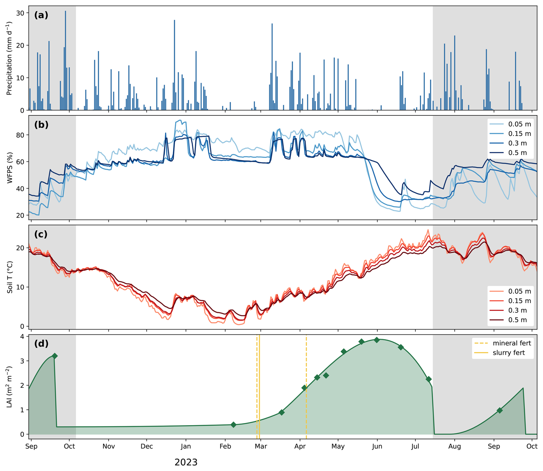
Figure 2 Environmental conditions and vegetation dynamics at the Oensingen cropland from September 2022 to October 2023. The unshaded area corresponds to the winter wheat cropping season, while the shaded areas indicate the final phase of the preceding temporary grassland and the cover crop following the winter wheat harvest. (a) Daily precipitation sums; (b) daily average water-filled pore space (WFPS) at 0.05, 0.15, 0.3, and 0.5 m soil depths; (c) daily average soil temperature (soil T) at the same depths as WFPS; (d) leaf area index (LAI), with diamonds indicating measured values and the line representing modelled values obtained using cubic splines. Yellow lines indicate fertilization (fert) events.

3.2 Greenhouse gas fluxes

3.2.1 Net ecosystem CO₂ exchange (NEE)

During the final regrowth phase of the temporary grassland in September 2022, daily mean NEE fluctuated around zero (−2.2 to +3.9 µmol CO₂ m⁻² s⁻¹; Fig. 3a). After the final grassland cut, NEE became positive, indicating a net release of CO₂. Herbicide application and direct seeding of winter wheat in early October 2022 further increased NEE, which reached a daily mean of +6.1 µmol m⁻² s⁻¹. In late October 2022, NEE gradually declined in response to decreasing soil temperature (Fig. 2c) and remained low but positive during the winter months (December 2022 to February 2023), reflecting a small net release of CO₂. From early March 2023 onward, NEE decreased and became negative, indicating the onset of net CO₂ uptake. During peak crop growth in early May, daily mean NEE reached −10.5 µmol m⁻² s⁻¹, and the most negative half-hourly flux (QC0) was −48.2 µmol m⁻² s⁻¹. Following anthesis and the onset of dry soil conditions at the end of May (Fig. 2b), NEE steadily increased, consistent with declining photosynthetic activity during wheat maturation. A small CO₂ emission peak, with daily mean NEE reaching up to +3.7 µmol m⁻² s⁻¹, occurred in late June, following rewetting after an extended dry period. From July to late August 2023, daily mean NEE remained positive (+1.9 to +7.7 µmol m⁻² s⁻¹), indicating net CO₂ release during late wheat maturation, after harvest and cover crop establishment. In late August, NEE became negative, reflecting net CO₂ uptake due to the successful establishment of the cover crop, before returning positive after mulching and soil tillage in late September.

3.2.2 N₂O fluxes

N₂O fluxes showed pronounced temporal variations, with low fluxes during winter 2022/2023 and highest emissions during crop establishment and after fertilization events. During the final grassland regrowth phase, daily mean N₂O fluxes were negligible (−0.3 to +0.6 nmol m⁻² s⁻¹; Fig. 3a), but increased markedly after winter wheat seeding, reaching +5.7 nmol m⁻² s⁻¹ on 22 October 2022 (Fig. 3b). This peak occurred after rainfall increased topsoil WFPS from 51 % to 62 % (Fig. 2b), while soil temperature remained above 14 °C (Fig. 2c) and LAI was still below 1 m² m⁻² (Fig. 2d). Throughout the winter (December 2022 to February 2023), N₂O fluxes remained near zero (−0.1 to +0.9 nmol m⁻² s⁻¹). Following the first fertilization events on 27 and 28 February, which supplied 111 kg N ha⁻¹ (total N; Table 1), N₂O fluxes increased sharply and exhibited three distinct peaks in March. The first peak occurred shortly after fertilization, reaching a daily mean flux of +6.2 nmol m⁻² s⁻¹ on 2 March, with topsoil WFPS above 65 %, soil temperature below 5 °C, and LAI still below 1 m² m⁻². A second, larger peak followed approximately ten days later, reaching a daily mean flux of +13.6 nmol m⁻² s⁻¹ on 12 March and a maximum half-hourly flux (QC0) of +27.8 nmol m⁻² s⁻¹. A third, smaller peak occurred at the end of March, reaching +4.0 nmol m⁻² s⁻¹ on 28 March. The second and third peaks were preceded by precipitation events that raised topsoil WFPS above 80 %, with soil temperature ranging from 5 to 10 °C, while LAI exceeded 1 m² m⁻² only during the last peak. After the last fertilization on 6 April (27 kg N ha⁻¹; Table 1), N₂O fluxes increased again, reaching a daily mean of +5.1 nmol m⁻² s⁻¹ on 14 April, under high topsoil WFPS (> 80 %; Fig. 2b) and a more developed canopy than during the March peaks (Fig. 2d). During peak crop growth period, when LAI increased from 2.5 to 4 m² m⁻² (mid-April to late May; Fig. 2d), daily mean N₂O fluxes remained negligible (−0.4 to +1.4 nmol m⁻² s⁻¹), despite relatively high WFPS (above 60 % throughout the soil profile) and increasing soil temperature. A short-lived emission event occurred after rewetting on 19 June, following the dry period in May and June. Despite WFPS remaining below 40 %, daily mean N₂O fluxes reached +11.2 nmol m⁻² s⁻¹ on 20 June, with a maximum half-hourly flux (QC0) of +21.6 nmol m⁻² s⁻¹, when LAI was already declining after anthesis. In July, during late wheat maturation and after harvest, N₂O fluxes remained low but positive (0.0 to +3.1 nmol m⁻² s⁻¹). A distinct peak occurred shortly after cover crop sowing, with a daily mean flux of +7.3 nmol m⁻² s⁻¹ on 30 July. Fluxes remained low in August (0.0 to +2.3 nmol m⁻² s⁻¹) but increased slightly again following mulching of the cover crop and soil tillage in late September 2023.

3.2.3 CH₄ fluxes

CH₄ fluxes remained low throughout the measurement period, typically indicating small CH₄ emissions, with daily average fluxes ranging from −7.0 to +28.5 nmol CH₄ m⁻² s⁻¹ (Fig. 3c). Higher CH₄ emissions occurred from mid-October to early November 2022 as well as in January 2023, while weak CH₄ uptake occurred during the dry period in May and June. The mean measured CH₄flux during the measurement period was +0.77 ± 8.57 nmol CH₄ m⁻² s⁻¹, with a median signal-to-noise ratio of 1.55, calculated as the flux record divided by its random uncertainty (estimated following Finkelstein and Sims, 2001), indicating weak net CH₄ exchange that was only marginally distinguishable from measurement noise.

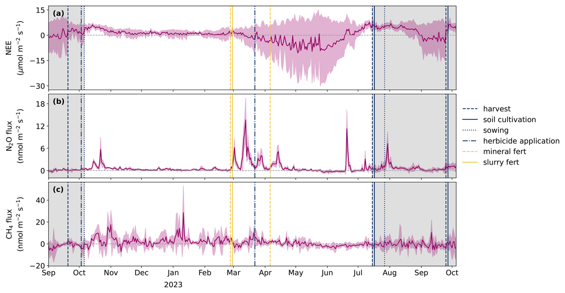
Figure 3 Gap-filled greenhouse gas fluxes at the Oensingen cropland measured from September 2022 to October 2023. The unshaded area corresponds to the winter wheat cropping season, while the shaded areas indicate the final phase of the preceding temporary grassland and the cover crop following winter harvest. (a) Net ecosystem CO₂ exchange (NEE), (b) N₂O fluxes, and (c) CH₄ fluxes. Fluxes were gap-filled using the Marginal Distribution Sampling (MDS) for NEE and random forest (RF) for N₂O and CH₄fluxes. Lines represent daily averages of the gap-filled half-hourly fluxes, while the shading indicates ±1 SD. Vertical lines mark management activities: yellow dashed = mineral fertilization (fert), yellow solid = slurry fertilization (fert), blue solid = soil cultivation, blue dotted = sowing, blue dashed = harvest, and blue dash-dot = herbicide application. See Table 1 for details on management activities.

3.3 Net greenhouse gas exchange and net GHG budget

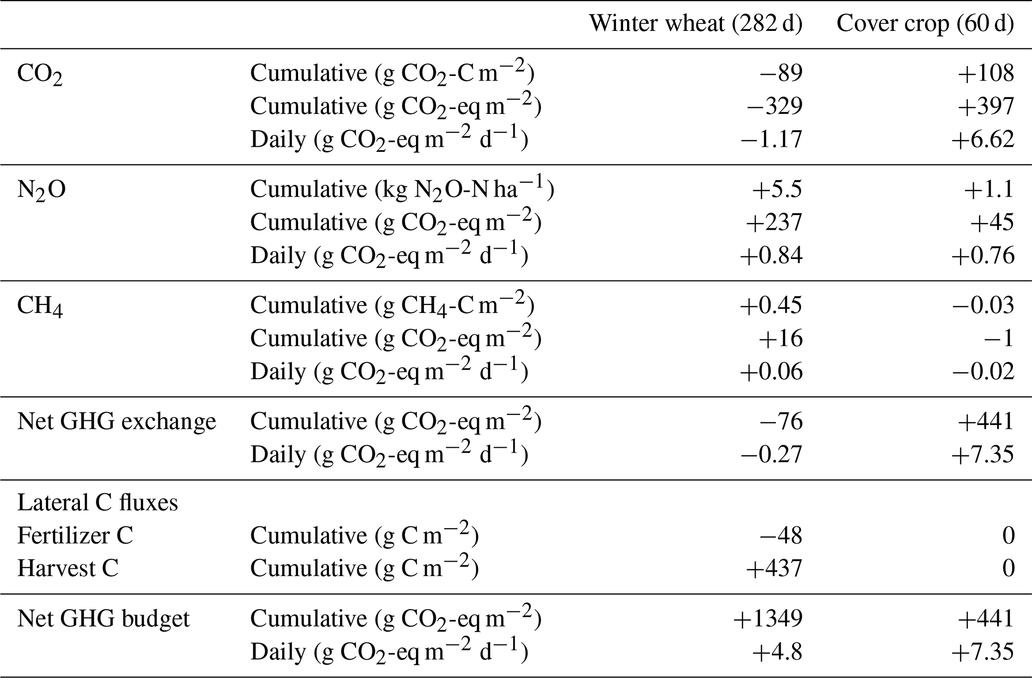
During the winter wheat cropping season (282 d), cumulative N₂O emissions were 5.5 kg N₂O-N ha⁻¹ (Table 2), with an average gap-filled flux of 0.81 nmol m⁻² s⁻¹. When scaled to crop yield, this corresponded to 1.1 kg of N₂O-N emitted per ton of wheat grain (dry matter). Based on the total N input from fertilizers of 138 kg N ha⁻¹ (Table 1), the resulting apparent emission factor (EF) was 4.0 %. Over the one-year period starting at winter wheat sowing, cumulative N₂O emissions amounted to 7.0 kg N₂O-N ha⁻¹, corresponding to an annual apparent EF of 5.1 %. Because no unfertilized control treatment was available, both values also reflect N₂O emissions from sources other than fertilizer application, such as those associated with mineralization of residues from the preceding grass-clover ley. During the subsequent 60 d cover crop season, cumulative N₂O emissions reached 1.1 kg N₂O-N ha⁻¹, and the average daily sum of N₂O emissions (17.6 g N₂O-N ha⁻¹ d⁻¹) was only slightly lower than that observed during the winter wheat season (19.6 g N₂O-N ha⁻¹ d⁻¹).

Throughout the winter wheat cropping season, the ecosystem acted as a net CO₂sink, with a cumulative NEE of −89 g CO₂-C m⁻² (Table 2). When expressed in CO₂-equivalents, concurrent N₂O emissions offset approximately 70 % of this seasonal net CO₂ uptake, while CH₄ emissions remained negligible. The resulting net GHG exchange (NGHGE) was therefore slightly negative, representing a small GHG sink with −76 g CO₂-eq m⁻². In contrast, the short summer cover crop period represented a net CO₂ source, emitting 108 g CO₂-C m⁻². N₂O emissions during this period accounted for approximately 10 % of NGHGE, while the net CH₄ exchange was again negligible. The NGHGE during the cover crop period showed large net GHG emissions (+441 g CO₂-eq m⁻²). The difference between the two crops was even more pronounced when comparing their daily NGHGE, with winter wheat averaging −0.27 g CO₂-eq m⁻² d⁻¹ and the cover crop averaging +7.4 g CO₂-eq m⁻² d⁻¹, resulting in a daily difference of approximately 8 g CO₂-eq m⁻² d⁻¹ (Table 2). However, when lateral C fluxes were included to calculate the net GHG budget, winter wheat was a substantial net GHG source (+1349 g CO₂-eq m⁻²), due to its large C export with harvested grain and straw, while the cover crop was a smaller net GHG source (+441 g CO₂-eq m⁻²; note: numbers are identical to NGHGE because no lateral C fluxes occurred). Sensitivity analysis across alternative u_* thresholds (CUT16, CUT84) showed a NGHGE spread of 82 g CO₂-eq m⁻² for winter wheat versus 26 g CO₂-eq m⁻² for the cover crop, driven mainly by CO₂ fluxes (Table A3).

Table 2 Cumulative greenhouse gas (GHG) fluxes, net GHG exchange (NGHGE), lateral C fluxes, and net GHG budget for the winter wheat and cover crop cropping seasons (282 and 60 d, respectively). NGHGE represents the EC-based sum of CO₂, N₂O, and CH₄ fluxes, expressed in CO₂-equivalents. The net GHG budget additionally includes lateral C inputs from organic fertilizer and C exports with harvest (grain and straw), with all fluxes converted to CO₂-equivalents using the molecular mass ratio of CO₂ to C. Negative values indicate net uptake or C input to the ecosystem, whereas positive values indicate net release or C export. CO₂-equivalents (g CO₂-eq m⁻²) for N₂O and CH₄ were calculated using global warming potentials (GWP₁₀₀) of 273 and 27, respectively, applied to fluxes expressed in g m⁻² (IPCC, 2021).

3.4 Drivers of N₂O flux dynamics over time

3.4.1 Temporal development of N₂O flux driver contributions

We used SHAP to quantify both the magnitude and direction (positive or negative) of each driver's contribution to N₂O fluxes across the measurement period, relative to a baseline. The SHAP baseline and thus the corresponding expected N₂O flux, when 30 d after fertilization and soil preparation were excluded, was estimated at 0.45 nmol N₂O m⁻² s⁻¹. To assess the overall influence of each driver across the study period, we summed up the SHAP values over time, separately for positive and negative contributions. This approach avoided cancelling out opposing effects and revealed how strongly each driver enhanced or decreased N₂O emissions (Fig. A3). N fertilization and soil disturbance increased the N₂O fluxes (i.e., positive SHAP values) relative to the baseline. In contrast, soil moisture, soil temperature, and GPP exhibited both positive and negative SHAP values, reflecting their capacity to either increase or decrease N₂O fluxes depending on environmental conditions. Across the study period (September 2022 to October 2023), N fertilization was the dominant driver increasing N₂O fluxes (43 % of all positive contributions), while soil moisture (19 %), GPP (17 %), soil disturbance (12 %), and soil temperature (9 %) also contributed to positive deviations from the baseline flux. Conversely, soil moisture (41 % of all negative contributions), GPP (30 %), and soil temperature (29 %) showed substantial negative contributions, indicating periods when these variables reduced N₂O fluxes relative to the baseline. SHAP dependence plots further showed that high recent N input, short time since fertilization or since soil preparation, high-WFPS episodes, and warmer soil conditions were generally associated with positive SHAP values of the respective driver, i.e. increased N₂O fluxes (Fig. A4).

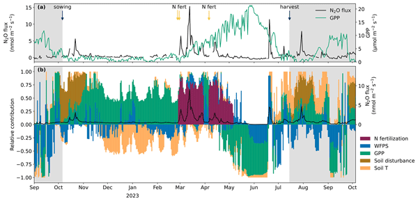
To assess the relative influence of each driver in a time-resolved manner and independently of the absolute magnitude of predictions, we computed daily averages of normalized SHAP values (see Sect. 2.7.2). These relative driver contributions revealed distinct temporal patterns across the study period (September 2022 to October 2023; Fig. 4). In September 2022, during the final grassland regrowth phase, N₂O emissions were mainly suppressed by WFPS (negative relative contributions; Fig. 4), although low GPP exerted a positive effect later in the month. At the beginning of October, herbicide application and the direct seeding of wheat introduced soil disturbance, and N₂O fluxes during crop establishment were primarily driven by soil disturbance and low GPP (positive relative contributions). Throughout the winter (November 2022 to February 2023), low soil temperatures consistently reduced N₂O emissions, while low GPP (Fig. 4a), reflecting limited crop activity and hence plant N uptake, maintained a positive effect on N₂O fluxes. In spring (March to April 2023), which corresponded to the period of highest observed N₂O fluxes (Fig. 4a), emissions were primarily driven by N fertilization, followed by WFPS. Later in the season, when photosynthetic activity and presumably plant N demand increased (April), the effect of GPP shifted towards decreasing N₂O fluxes. The low N₂O emissions observed from May to mid-June were thus strongly driven by large negative effects of GPP and WFPS (Fig. 4b). In contrast, during grain filling and post-harvest (July to mid-August), the SHAP analysis indicated that soil temperature, soil disturbance, and low GPP increased N₂O emissions. Following the establishment of the cover crop in September, the effect of GPP became negative again, coinciding with an increase in photosynthetic CO₂ uptake.

The SHAP dependence plot for GPP showed a clear shift from mostly positive SHAP values at low GPP to increasingly negative SHAP values at higher GPP (Fig. 5). Thus, low crop activity was generally associated with higher predicted N₂O fluxes, whereas periods of greater crop activity were associated with lower predicted N₂O fluxes.

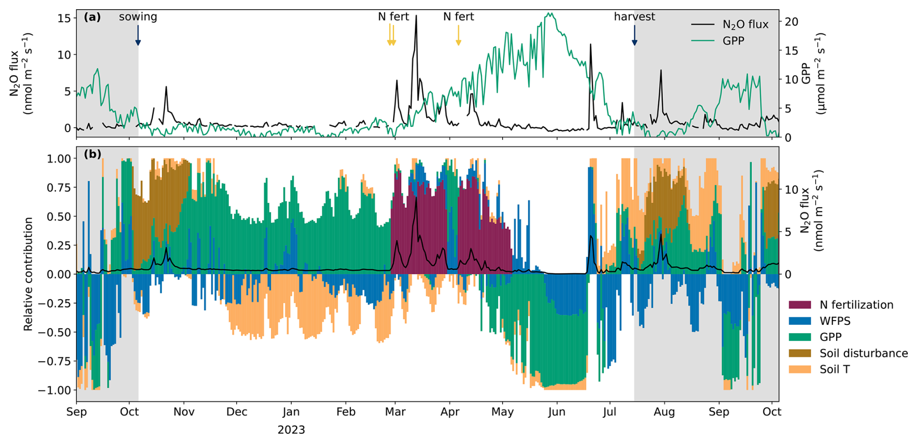
Figure 4 Temporal dynamics of N₂O fluxes, gross primary productivity (GPP), and relative driver contributions to N₂O fluxes at the Oensingen cropland from September 2022 to October 2023. The unshaded area corresponds to the winter wheat cropping season, while the shaded areas indicate the final phase of the preceding temporary grassland and the cover crop following winter harvest. (a) Daily average N₂O fluxes (measured, highest quality fluxes only) are shown in black, and daily average GPP in green. Arrows at the top denote management activities conducted during the winter wheat cropping season. (b) Relative contributions of individual drivers (i.e., N fertilization, water-filled pore space (WFPS), GPP, soil disturbance, and soil temperature (soil T)) are expressed as daily averages of normalized SHAP values (see Sect. 2.7.2 for methodological details). The baseline (SHAP = 0) corresponds to a predicted N₂O flux of 0.45 nmol m⁻² s⁻¹. Positive values indicate that a driver raised N₂O fluxes above the baseline flux, negative values that it lowered them below. The black line represents the model-predicted N₂O flux.

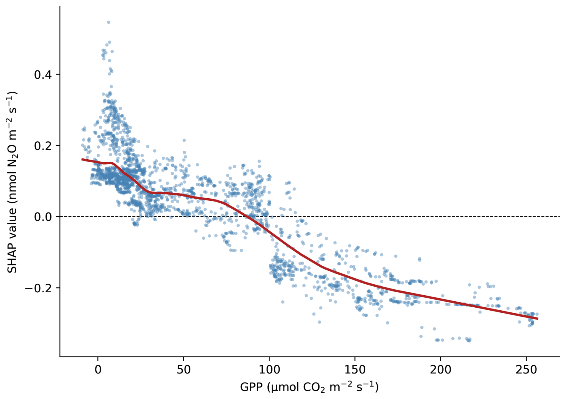
Figure 5 SHAP dependence plot showing the SHAP value of GPP (rolling sum over the preceding 48 h) against its observed values across all data, reflecting GPP's marginal contribution to the modelled N₂O fluxes. A LOWESS smoother (red line) is overlaid to highlight the overall trend.

3.4.2 Soil available nitrogen

To assess soil N availability to roots and microorganisms, we used two complementary approaches: (i) time-integrated supply of plant-available NO${}_{\mathrm{3}}^{-}$-N measured with PRS probes, and (ii) instantaneous mineral N pools (N_min), derived from soil-extractable NO${}_{\mathrm{3}}^{-}$ and NH${}_{\mathrm{4}}^{+}$concentrations in the 0–0.3 m soil layer. N₂O fluxes increased significantly with soil mineral N availability, both for integrated (Fig. 6c, R²=0.61; p<0.05) and instantaneous supply (Fig. 6d; R²=0.77; p<0.05). The lowest N₂O emissions occurred during periods of highest GPP (point 4 in Fig. 6c; point D in Fig. 6d) or without prior fertilization events (points A and B in Fig. 6d). In contrast, the highest N₂O emissions occurred after fertilization events, when soil mineral N availability was highest (points 1 and 2 in Fig. 6c; point C in Fig. 6d), with average Nmin values reaching 74 kg N ha⁻¹ ten days after the first fertilization. Between these extremes, intermediate N availability was observed in December 2022 (point A in Fig. 6d) and in August 2023 during the post-harvest period (points 6 and 7 in Fig. 6c; point E in Fig. 6d). While in August the intermediate N availability coincided with higher N₂O emissions, this was not the case in December, when soil temperature at 0.05 m depth ranged between 3 and 5 °C during the sampling week.

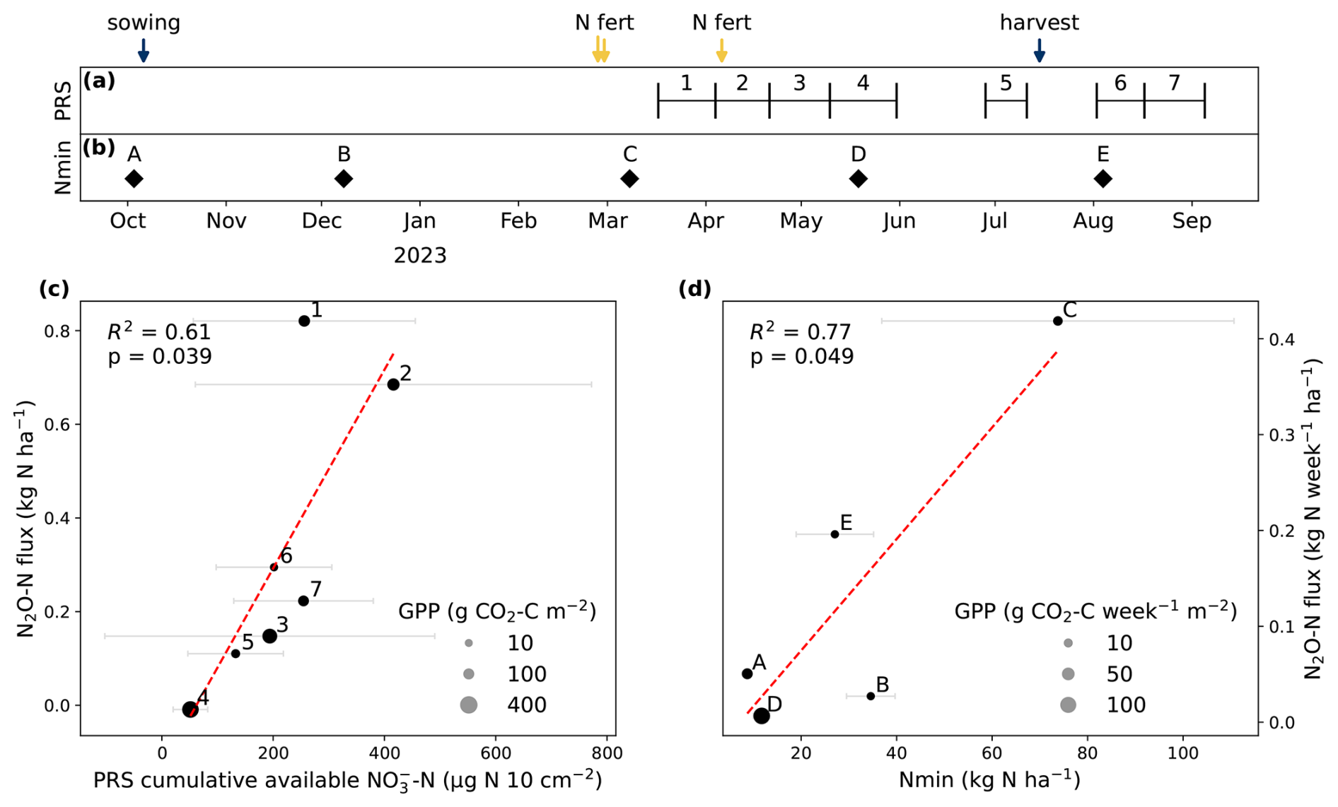
Figure 6 Relationships between nitrogen (N) availability and N₂O fluxes. (a) Timeline of burial periods for plant root simulators (PRS) probes, and (b) of soil mineral N (N_min) sampling campaigns. Sowing, harvest, and fertilization dates are also provided. (c) Relationship between cumulative available NO${}_{\mathrm{3}}^{-}$-N (µg N 10 cm⁻², based on PRS probes) and cumulative N₂O fluxes over the corresponding burial period (15 to 21 d). Means and ±1 SD are given (n=5). Circle size reflects cumulative GPP during the same period. Numbers indicate the corresponding period as shown in panel (a). A linear regression is shown as a dashed red line, together with the coefficient of determination (R²) and corresponding p-value. (d) Relationship between N_min (0–0.3 m soil depth) and cumulative N₂O fluxes during the week centered on the soil sampling (±3.5 d). Means ±1 SD are given (n=4; except for 1st sampling with no replicates). Circle size reflects cumulative GPP during the same period. Letters indicate the corresponding period as shown in panel (b). A linear regression is shown as a dashed red line, together with the coefficient of determination (R²) and corresponding p-value.

3.5 N₂O-producing processes inferred from stable isotopes

We used stable oxygen and nitrogen isotopes to identify the microbial processes underlying the measured N₂O fluxes during the three weeks following the first fertilization events on 27 and 28 February 2023. The δ¹⁸O and site preference (SP-N₂O) of emitted N₂O ranged between 17.3 ‰ and 39.8 ‰ and from −7.2 ‰ to +18.2 ‰, respectively (Fig. 7a). The dual isotope plots suggested that heterotrophic bacterial denitrification and/or nitrifier denitrification were the dominant N₂O production pathways (Figs. 7a, A5). Moreover, the observed trend of increasing enrichment of δ¹⁸O and SP-N₂O over time (Fig. 7a) suggested isotopic fractionation associated with the microbial reduction of N₂O to N₂ during denitrification. Results from the FRAME model supported the qualitative source attribution derived from the isotope mapping approach and enabled the quantification of both the relative contributions of individual N₂O-producing processes and the extent of N₂O reduction to N₂. However, following Buchen et al. (2017), we pooled heterotrophic bacterial denitrification with nitrifier denitrification, and nitrification with fungal denitrification, due to the large uncertainty in separating these processes given their similar endmembers. All four processes are nonetheless shown separately in Fig. A6. N₂O fluxes decreased during the sampling period (Fig. 7b), whereas the source contributions showed no clear temporal trend (Fig. 7c). Heterotrophic bacterial denitrification and/or nitrifier denitrification dominated N₂O production throughout the sampling period, contributing 74 %–86 % (±9 %–21 %) across the four sampling dates (Fig. 7c; based on the mixing-reduction scenario), while nitrification and/or fungal denitrification accounted for the remaining 14 %–26 %. The alternative reduction-mixing scenario produced very similar source-fraction distributions, with only slightly higher reduced N₂O fractions, while the overall interpretation remained unchanged (Fig. A6). The reduced N₂O fraction, reported as (1−r), remained between 40 % and 47 % on the first three sampling dates and increased markedly to 78 ± 13 % on 17 March, indicating a larger fraction of N₂O reduced to N₂ at the end of the sampling period, coinciding with decreasing chamber-based N₂O fluxes (Fig. 7b).

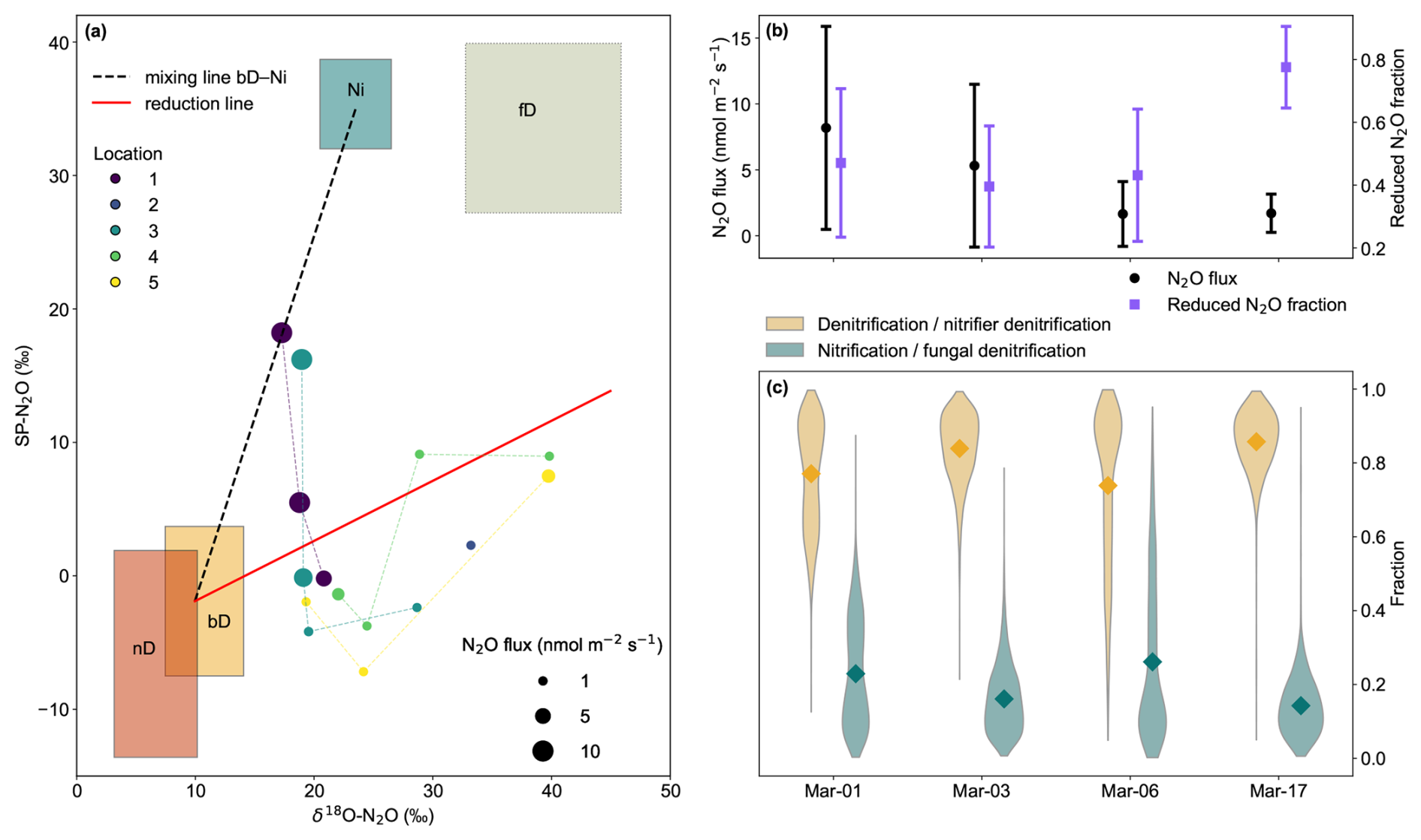
Figure 7 Isotopic signature of N₂O, N₂O flux magnitudes, and their estimated source fractions in March 2023, following fertilization applied on 27 February (ammonium-nitrate) and 28 February (slurry). (a) Dual isotope plot of δ¹⁸O-N₂O vs. site preference (SP-N₂O). Colored boxes denote endmembers for the N₂O mixing (nD: nitrifier denitrification, bD: heterotrophic bacterial denitrification, Ni: nitrification, fD: fungal denitrification). Endmember values of boxes are derived from Yu et al. (2020) and adjusted to the values of soil water (δ¹⁸O-H₂O = −9.2 ‰) at the study site (except for the Ni box). Lines for mixing (black) and N₂O reduction to N₂ (red) are shown. Individual measurements are shown as circles, with size reflecting flux magnitude and color indicating location (1 to 5; see Fig. 1). (b) N₂O fluxes measured with static chambers (black) and the fraction of N₂O reduced to N₂ estimated by the FRAME model (purple). The latter is expressed as (1−r), where r denotes the residual unreduced N₂O fraction. N₂O fluxes are shown as means ±1 SD across the chambers for which isotope data were available, whereas reduced N₂O fractions are shown as means ±1 SD across all FRAME simulations based on those chamber measurements. (c) N₂O source fractions estimated by the FRAME model, based on the mixing-reduction scenario, for heterotrophic bacterial denitrification and nitrifier denitrification vs. nitrification and fungal denitrification, displayed as violin plots, with mean values indicated by diamonds (see text for details).

4 Discussion

4.1 Explainable machine learning for analysing N₂O flux dynamics

Two central objectives of this study were to quantify N₂O fluxes and determine when and how environmental and management drivers affected these fluxes during a winter wheat cropping season and the subsequent cover crop season. To address these objectives, we used an explainable ML framework (i.e., XGBoost-SHAP) as an interpretative tool to extract, from high-frequency EC observations, the temporal development of driver contributions to N₂O fluxes. We preferred tree ensembles over recurrent architectures such as long short-term memory networks, which can capture lagged driver-response relationships directly but require more data than a single site-year provides (Hamrani et al., 2020). Temporal dependencies were therefore represented through explicit feature engineering in our study. Such a framework offers several advantages over traditional statistical models. First, N₂O fluxes are highly episodic and respond non-linearly to interacting drivers, conditions under which ML models are expected to outperform linear models (Gnisia et al., 2025; Hamrani et al., 2020). Second, SHAP values allowed us to quantify not only the average importance of each driver, but also how its contribution evolved over time. Third, XGBoost captures interactions among drivers intrinsically through the hierarchical structure of the tree splits, without interaction terms needing to be specified a priori. Fourth, this framework enabled us to incorporate management history alongside continuous biophysical drivers, enabling interpretation of management effects not possible with classical statistical analyses.

As with any data-driven approach, these advantages come with trade-offs. SHAP quantifies how each driver contributes to the model's predictions rather than establishing process-based causal effects, and it can attribute variance only to predictors that are included. Two key drivers were not explicitly represented in our ML model: soil N mineralization and the availability of labile organic C. Their influence was therefore likely redistributed onto other predictors. Thus, effects of the mineralization of residues from the preceding grass-clover ley likely extended beyond the 30 d windows used here to represent soil disturbance, while the effect of labile organic C supplied with the slurry could not be separated from that of the fertilizer N and was therefore attributed to the engineered fertilization variables. Nevertheless, high-resolution environmental, management, and EC data over a full year provided a sound basis for the XGBoost-SHAP framework in this study, within clear limits. The model reproduced the timing of the main emission episodes but underestimated peak magnitudes and overestimated low fluxes, and it explained a moderate share of the variance in the independent hold-out period (R²=0.36; Fig. A2). Some temporal patterns of the modelled contributions might also reflect how predictors were constructed rather than changes in the underlying processes. For example, the fertilization and soil disturbance variables were engineered based on prior knowledge to represent a 30 d effect, so some driver contributions shifted abruptly once that window elapsed (Fig. 4b, e.g., early April and early May). SHAP attributions were nonetheless generally consistent with established process understanding and published field studies (see Sect. 4.2).

These trade-offs also delimit what an empirical ML framework can and cannot replace. Process-based biogeochemical models explicitly represent soil N and C pools and related transformations, allowing them to simulate hypothetical management scenarios and extrapolate beyond observed conditions, though their ability to reproduce N₂O fluxes and their short-term variation remains limited (Saha et al., 2021; Scheer et al., 2025). ML models cannot represent the underlying pools and instead describe the conditions under which N₂O fluxes occurred, but they require no site-specific parameterization and can exploit the full temporal resolution of EC data. Both approaches are therefore complementary rather than competing. Comparing SHAP-identified driver responses against the sensitivity of a process-based model to the same drivers can provide an independent check on whether the empirical attributions are mechanistically plausible. Furthermore, a limitation of our own setup points to a way forward: soil mineral N could not be used as a predictor because it was measured only on discrete dates (Sect. 2.7.1), whereas a calibrated process-based model could supply continuous simulated N_min and mineralization rates as ML predictors, replacing the engineered fertilization and soil disturbance proxies used here. Integrating ML with process-based models (Saha et al., 2021; Sharma et al., 2026) and adopting knowledge-guided ML approaches (Liu et al., 2022) are therefore promising next steps to address the complexity of N₂O emissions from managed ecosystems.

4.2 Seasonal changes in N₂O fluxes and their drivers

Two periods emerged as particularly relevant for N₂O emissions: crop establishment and early spring. Both were characterized by a mismatch between N supply and plant demand, with substantial mineral N supply from mineralization or fertilization coinciding with limited crop uptake, resulting in surplus soil mineral N, that under favorable moisture and temperature conditions, fuelled microbial N₂O production.

During crop establishment, elevated emissions were affected by soil disturbance and low crop activity (i.e., low GPP). Herbicide termination of the temporary grassland and direct seeding of winter wheat likely stimulated mineralization of soil organic matter and crop residues, as indicated by increased NEE (intensified soil respiration), while low GPP reflected limited plant N uptake (Fig. A1). Together, these processes raised soil N_min from 8.7 to 34.6 kg N ha⁻¹ between October and early December 2022 (0–0.3 m soil depth; Fig. 6d), consistent with observations after grassland termination (Beiküfner et al., 2025; Buchen et al., 2017; Helfrich et al., 2020). A comparable response occurred during cover-crop establishment after wheat harvest, when warm soil temperatures and soil tillage enhanced mineralization (Grandy and Robertson, 2006) and N_min rose from 12 to 27 kg N ha⁻¹ between late May and early August (Fig. 6d). Thus, management practices that leave soils disturbed and poorly vegetated favored N₂O emissions at our site, consistent with previous work suggesting that rapid and sustained soil cover, e.g. through optimized sowing dates, cover crops or cultivar choice, can reduce emissions during such periods (Maier et al., 2025; Quemada et al., 2020; Tallec et al., 2022).

In early spring, high N₂O emissions were predominantly driven by N fertilization, with WFPS contributing during peak events. The first fertilizer applications in late February combined mineral (NH₄NO₃) and organic (slurry) N, supplying a large N input (111 kg N ha⁻¹) at tillering, which coincided with high soil moisture, conditions typical for central European climates (Ruosteenoja et al., 2018). At this stage, low LAI (Fig. 2d) and low GPP (Fig. 4a) indicated limited plant N demand, so that soil N_min reached 74 kg N ha⁻¹ (Fig. 6d), which, together with precipitation events (Fig. 2a), created optimal conditions for microbial N₂O production. By contrast, the smaller final fertilization in early April (27 kg N ha⁻¹) was applied during stem elongation, when plant N demand was higher, as indicated by increased LAI (∼ 2 m² m⁻²) and GPP, which likely reduced substrate availability for N₂O production. Mitigation practices in such periods will depend on better synchronizing fertilizer N inputs with crop demand and soil N mineralization, e.g. through adjusted fertilizer timing and amounts (Hoben et al., 2011; Omonode et al., 2017), split applications, site-specific planning (Jordan-Meille et al., 2023), precision fertilization (Diacono et al., 2013) or enhanced-efficiency fertilizers (Akiyama et al., 2010).

Over the entire study period, N fertilization was the dominant driver increasing N₂O fluxes (Fig. A3), consistent with its role as the primary source of reactive N in croplands (Shcherbak et al., 2014). WFPS, GPP, soil temperature, and soil disturbance made substantial but temporally varying contributions, underlining the multifactorial and interactive nature of N₂O emissions. WFPS had both positive and negative effects but consistently emerged as a key driver during peak emission events. GPP, used here as a proxy for crop activity and N demand, was clearly negatively associated with N₂O fluxes (Fig. 5). We interpreted this result as an indirect, plant-mediated effect, reflecting microbial substrate limitation: as the crop grows, its N uptake depletes soil mineral N available for microbial N₂O production (Abalos et al., 2018; Feigenwinter et al., 2023; Maier et al., 2022; Timilsina et al., 2024). Because WFPS was included in the model, an alternative pathway, i.e., high transpiration rates lowering soil moisture and thereby suppressing N₂O production, was already accounted for. Although root C exudation might favor denitrification (Philippot et al., 2009), the negative relationship suggests substrate limitation dominated. Overall, our results are consistent with the “N synchrony framework” (Cassman et al., 2002; Cassman and Dobermann, 2022): the highest N₂O losses coincided with the largest mismatch between N supply and crop N demand, in line with previous work linking N surplus to N₂O emissions (Van Groenigen et al., 2010; Tallec et al., 2022).

4.3 Cumulative N₂O losses and net GHG exchange

Cumulative N₂O emissions during the winter wheat season were 5.5 kg N₂O-N ha⁻¹, substantially exceeding the ranges reported for winter wheat by Garnier et al. (2024) for northern France (0.1–2.7 kg N₂O-N ha⁻¹) and by Tallec et al. (2022) for southwestern France (0.95–2.91 kg N₂O-N ha⁻¹), both chamber-based studies, although our N input (138 kg N ha⁻¹) was well within their reported fertilizer ranges. Yield-scaled N₂O emissions in our study (1.1 kg N₂O-N Mg⁻¹grain) were approximately three times higher than global values reported for wheat by Yao et al. (2024; 0.301–0.346 kg N₂O-N Mg⁻¹grain). Part of this discrepancy may be methodological, since global syntheses rely largely on soil chambers with lower spatial and temporal coverage than continuous EC, which better captures short-lived peaks and integrates fluxes over larger areas (Butterbach-Bahl et al., 2026). In addition to methodological differences, the elevated N₂O emissions in our study likely reflected site- and management-specific conditions. At our site, substantial amounts of mineral N were probably supplied by mineralization of residues from the preceding three-year grass-clover ley, as indicated by the accumulation of soil mineral N during autumn in the absence of any fertilization (Sect. 4.2). In addition, the near-simultaneous application of mineral N and slurry at the end of February likely created conditions particularly conducive to N₂O production, owing to the input of readily degradable carbon (Dittert et al., 2005; Schils et al., 2008). Poor drainage in the silty clay Eutric-Stagnic soil likely amplified both effects, favoring the high soil moisture and limited aeration under which denitrification proceeds.

To our knowledge, this is the first study to report EC-based N₂O fluxes over a complete winter wheat season. Notably, our N₂O emissions only slightly exceeded those observed for maize in Switzerland (with EC: 4.8 kg N₂O-N ha⁻¹; Maier et al., 2022), despite the much shorter maize season (127 vs. 282 d). The two crops also clearly differed in their N use efficiency (NUE, calculated as the ratio between N output to N input, not accounting for soil N mineralisation): winter wheat took up 113 kg N ha⁻¹ from an input of 138 kg N ha⁻¹ (NUE of 82 %), whereas maize took up only 56 kg N ha⁻¹ from an input of 110 kg N ha⁻¹ (NUE of 51 %; derived from Table 1 in Maier et al., 2022). The higher wheat NUE is consistent with Yu et al. (2022) and may partly reflect crop-specific differences (e.g., C3 vs. C4 traits, soil N dynamics, weather) but should be interpreted with caution since N supplied through mineralization of the preceding 3-year grass-clover ley was not captured in the fertilizer-N input term. So, the apparent NUE given above likely overestimates the true NUE.

The N₂O losses substantially affected the EC-based net GHG exchange (NGHGE) of the winter wheat season, with N₂O emissions offsetting 70 % of the seasonal net CO₂ uptake. This offset is considerably higher than those reported by Maier et al. (2022) for pea and maize in Switzerland (12 % and 10 %, respectively) and for managed Central European permanent grasslands (Hörtnagl et al., 2018). This large offset partly reflected the small net CO₂ sink during the winter wheat season, likely driven by enhanced heterotrophic respiration from decomposition of the preceding grass-clover ley residues. When including lateral C fluxes, i.e., organic fertilizer inputs and harvest exports, to calculate the net GHG budget, winter wheat was a substantial net GHG source, consistent with net C losses and declining SOC stocks reported from long-term measurements at the same site (Emmel et al., 2018). The field acted as a small net CH₄ source, consistent with results from other agricultural soils (Cowan et al., 2021). CH₄ emissions occurred mainly during wet periods, while dry periods showed low uptake, indicative of aerobic oxidation (Le Mer and Roger, 2001). The net CH₄ source likely reflected the poorly drained silty clay soil at our site, which likely promoted anaerobic conditions favoring methanogenesis.

Despite the absence of fertilizer application, the average N₂O flux during the cover crop season was only slightly lower than that during the winter wheat season (0.72 vs. 0.81 nmol m⁻² s⁻¹, respectively). This most likely reflected low plant N uptake due to slow crop establishment and enhanced N mineralization due to warm temperatures and post-harvest soil disturbance, as indicated by increased soil N_min between late May to early August (Fig. 6d). Such conditions are consistent with recent studies showing that bare or sparsely vegetated soils promote N₂O emissions through reduced plant N uptake and enhanced microbial activity (Maier et al., 2025; Shang et al., 2024; Tallec et al., 2022; Timilsina et al., 2024). Moreover, daily mean NEE remained positive until late August (Fig. 3a), indicating that the soil was a net CO₂ source for approximately half of the 60 d cover crop season. As a result, the cover crop season was characterized by net CO₂ release, accounting for 90 % of the total GHG budget during this period, with N₂O contributing the remaining 10 %, while CH₄ fluxes were negligible (Table 2). However, this net CO₂ release reflected NEE during a short, disturbed post-harvest establishment phase rather than an intrinsic property of cover crops: a summer cover crop between two winter cereals is not standard practice at this site and was implemented for the first time. Indeed, cover cropping reduced post-harvest GHG emissions relative to bare soil: in 2019, when the field was left bare after winter wheat harvest, daily post-harvest CO₂-eq fluxes were roughly double those measured during this study (16 vs. 7.4 g CO₂-eq m⁻² d⁻¹; Maier et al., 2025), driven primarily by increased CO₂ emissions. Although management and climatic conditions differed between the two years, this pronounced difference highlights the benefit of maintaining a green cover crop between two winter crops, also consistent with modelling results at the same site (Emmel et al., 2018) and current Swiss policy promoting continuous soil cover (Art. 71c DZV, Swiss Federal Council, 2025).

4.4 Temporal dynamics of N₂O source processes

Stable isotope sampling on selected dates in March 2023, following fertilizations on 27–28 February, coincided with the period of highest N₂O fluxes: cumulative EC-based emissions in March alone totalled 2.5 kg N₂O-N ha⁻¹, i.e. 45 % of the seasonal total for winter wheat. The FRAME model by Lewicki et al. (2022) allowed quantification of the relative contributions of different N₂O-producing processes over time. Denitrification, in particular heterotrophic bacterial denitrification, was the dominant source of N₂O (Figs. 7, A6), consistent with poor soil drainage and persistently high WFPS (> 65 % at 0.05 m), which promoted anaerobic conditions that favor denitrification (Bateman and Baggs, 2005; Davidson, 1991). Improving drainage in such settings may therefore help to mitigate N₂O emissions by reducing the extent and duration of waterlogging and the associated anaerobic conditions (Bouwman, 1996; Grossel et al., 2016). The low reduced N₂O fraction (∼ 40 %–50 %) in the week following fertilization may reflect elevated NO${}_{\mathrm{3}}^{-}$ concentrations, leading to NO${}_{\mathrm{2}}^{-}$ accumulation and inhibition of the final reduction step of N₂O to N₂ (Blackmer and Bremner, 1978; Senbayram et al., 2019). The fraction then increased markedly to ∼ 80 % on 17 March, coinciding with topsoil WFPS exceeding 80 %, thereby favoring complete denitrification. The near-simultaneous application of mineral N and slurry likely further promoted denitrification by providing both NO${}_{\mathrm{3}}^{-}$ and easily degradable organic C, creating conditions favorable for heterotrophic denitrifier activity (Dittert et al., 2005). Because such high-risk combinations can occur in mixed crop-livestock systems, policy and management guidance should discourage closely timed applications (Schils et al., 2008).

5 Conclusions

The XGBoost-SHAP framework proved to be an effective tool for identifying not only the main drivers of N₂O fluxes but also their temporal development, allowing the identification of critical periods for N₂O losses during a winter wheat season and the subsequent summer cover crop. Thanks to its flexibility and data-driven nature, this framework can be applied to other cropping systems to improve our understanding of N₂O emission dynamics and inform targeted management. Crop establishment and early spring emerged as particularly vulnerable phases for N₂O losses, largely due to a mismatch between N supply and plant demand. This lack of synchronization, driven by slow early crop development or early fertilization, led to elevated soil mineral N levels, which, under favorable moisture and temperature conditions, created hot moments of microbial N₂O production, primarily through denitrification. Elevated gross primary productivity (GPP, used as a proxy for crop activity and N demand) showed a consistent negative effect on N₂O fluxes, supporting the critical role active vegetation can play in limiting N₂O emissions. Both cumulative and yield-scaled N₂O emissions exceeded those reported in previous studies on wheat, most likely reflecting site-specific conditions such as the N legacy of the preceding ley as well as the higher temporal coverage of continuous flux measurements. This highlights the need for high-resolution N₂O flux measurements across a range of management, soil, and climate conditions to better constrain cropland GHG assessments.

Appendix A

Table A1 Management activities during the 2022–2023 measurement period at the cropland in Oensingen.

Table A2 Summary of data gaps in EC flux time series used in this study. Gap statistics are reported for two quality-control selections: QC0, including only best-quality records, and QC0-1, including best- and medium-quality records. Gap length is expressed in time steps (1 step = 30 min), with a “gap” being a contiguous sequence of missing records. Total number of gaps, median, third quartile (i.e., 75th percentile, Q3), and maximum gap length per time series are shown. Percentage of gaps that were shorter than one day, the number of gaps longer than three days, and the number of gaps longer than one week are given as well.

Table A3 Cumulative fluxes of CO₂, N₂O, and CH₄ (expressed in CO₂ equivalents) and the resulting net GHG exchange (NGHGE) for the winter wheat and cover crop seasons under three constant friction velocity (u_*) filtering thresholds (CUT), following Pastorello et al. (2020): the 16th percentile (CUT16), the default median threshold (CUT50), and the 84th percentile (CUT84) are given.

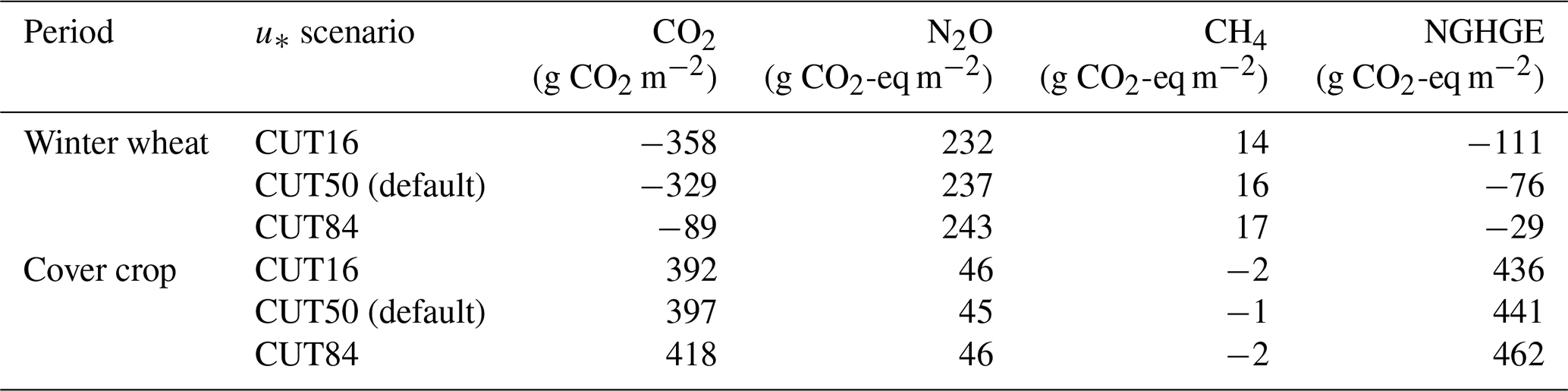
Table A4 Overview of key phenological stages of winter wheat, showing observation dates and corresponding BBCH growth stage numbers during the 2022–2023 growing season.

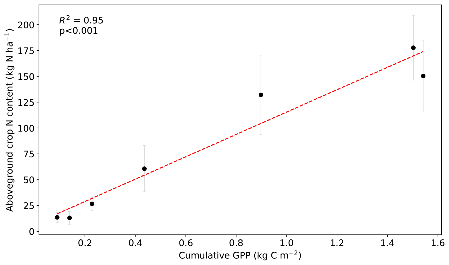
Figure A1 Relationship between cumulative gross primary productivity (GPP) and aboveground crop N content during the wheat growing season. Means ± 1 SD are given (n=12). The dashed red line indicates a linear least-squares regression, with the coefficient of determination (R²) and respective p-value shown.

Table A5 Optimized XGBoost hyperparameters for the N₂O flux driver model. Hyperparameters were selected using a randomized search with 5-fold cross-validation within the training dataset. The search evaluated 200 parameter combinations, corresponding to 1000 model fits in total. The best cross-validation RMSE was 1.85 nmol N₂O m⁻² s⁻¹.

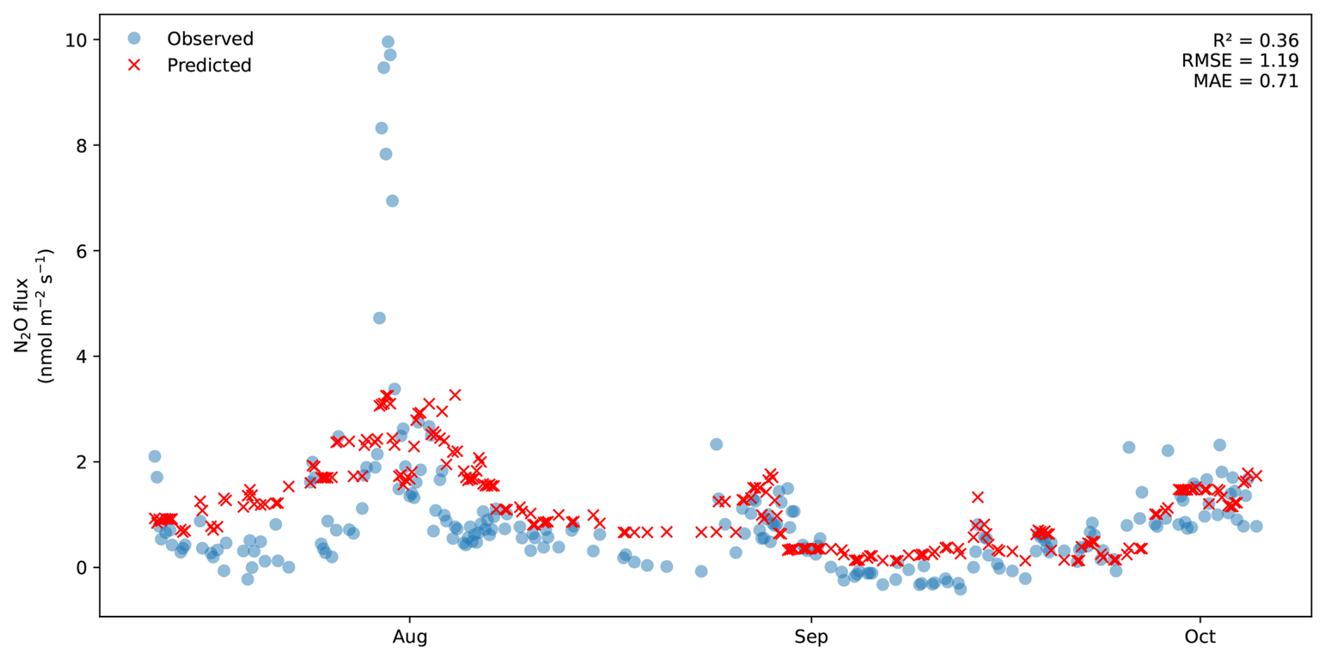
Figure A2 Observed and predicted N₂O fluxes at the cropland Oensingen for the independent chronological hold-out set, corresponding to the final 20 % of the time series. The blue circles represent the values predicted by the XGBoost model, while the red crosses indicate the observed values. The coefficient of determination (R²), root mean square error (RMSE), and mean absolute error (MAE) for the hold-out set are given.

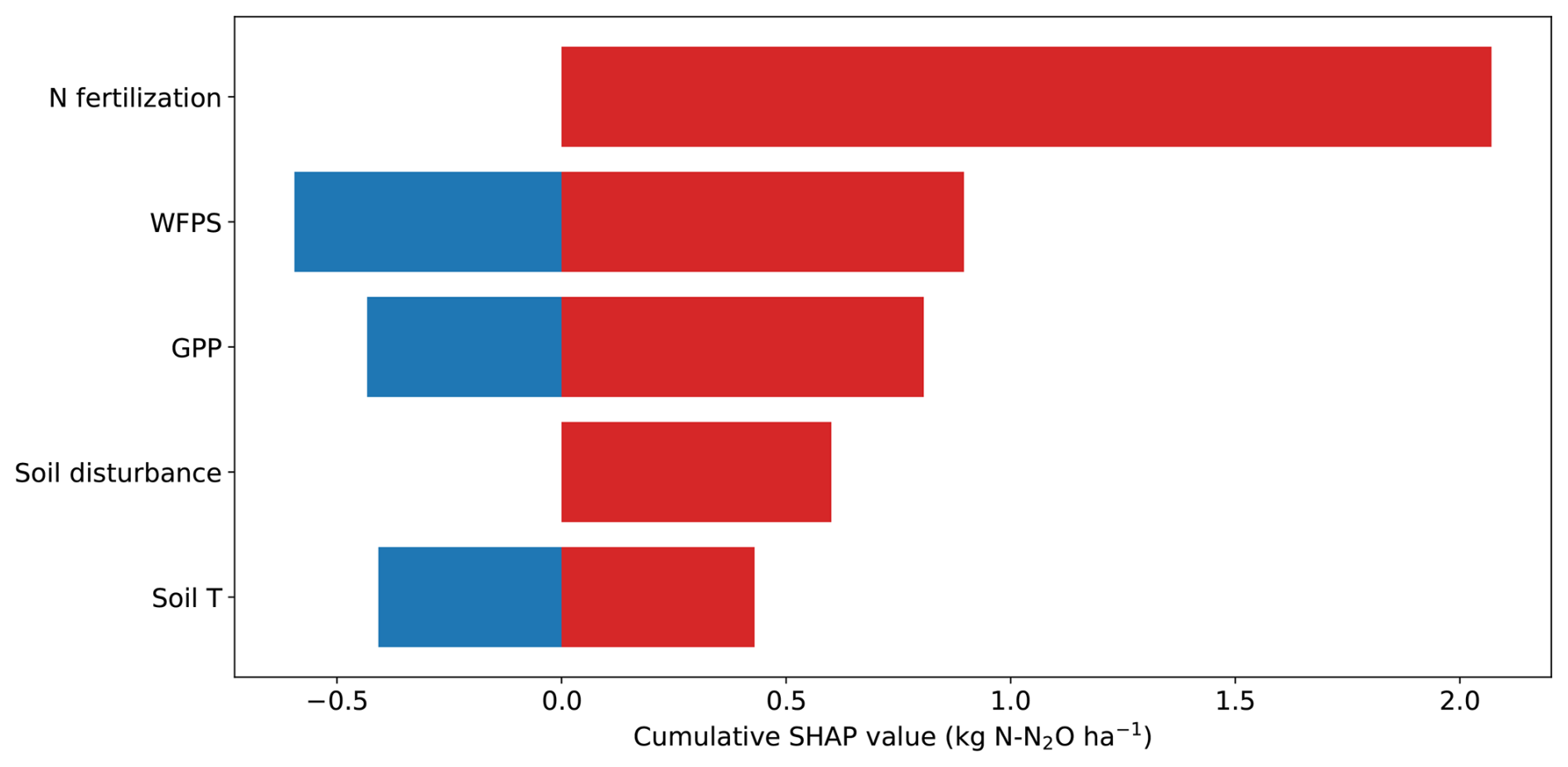
Figure A3 Cumulative positive (red) and negative (blue) SHAP contributions of each driver to predicted N₂O fluxes from September 2022 to October 2023 at the cropland Oensingen. Positive and negative SHAP values were summed up separately, such that increases and decreases in N₂O fluxes are shown independently rather than cancelling each other out.

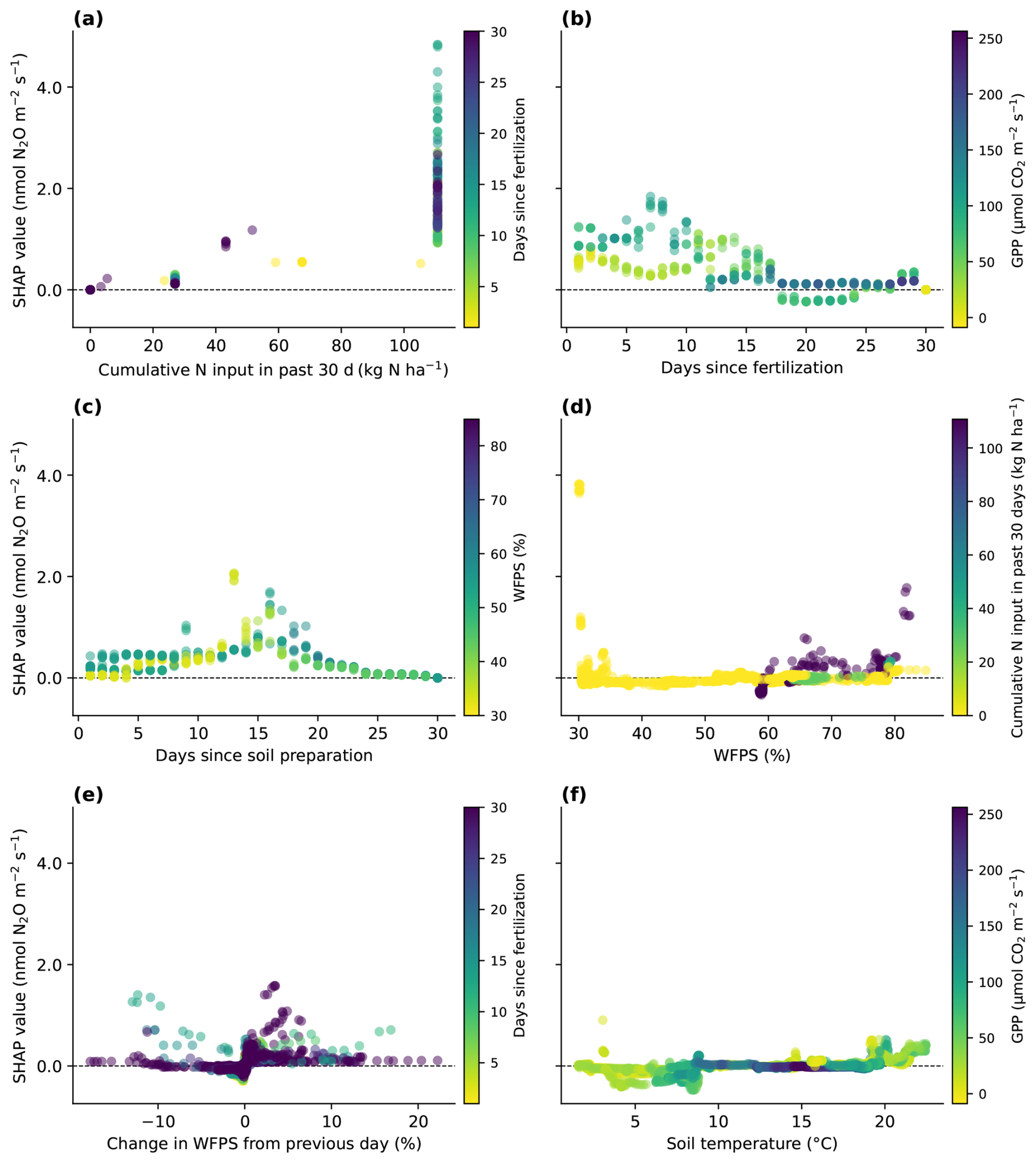
Figure A4 SHAP dependence plots for the drivers used in the XGBoost model for N₂O fluxes (except for GPP, which is shown separately in Fig. 5). Each panel shows the SHAP values of a given driver against its observed values across all data, reflecting the driver's marginal contribution to the modelled N₂O flux. Points are colored by a second driver.

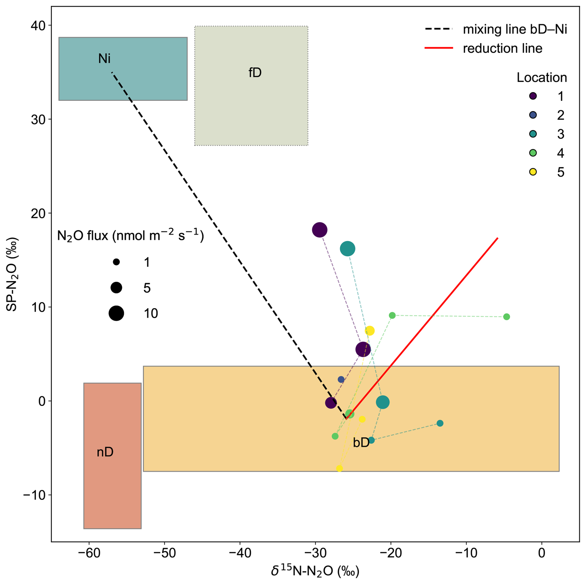
Figure A5 Dual isotope plot of δ¹⁵N^bulk-N₂O vs. site preference (SP). Colored boxes denote N₂O mixing endmembers (nD: nitrifier denitrification, bD: heterotrophic bacterial denitrification, Ni: nitrification, fD: fungal denitrification). Endmember values are derived from Yu et al. (2020). Lines for mixing (black) and N₂O reduction to N₂ (red) are shown. Individual measurements are shown as circles, with size reflecting flux magnitude and color indicating location (1 to 5; see Fig. 1).

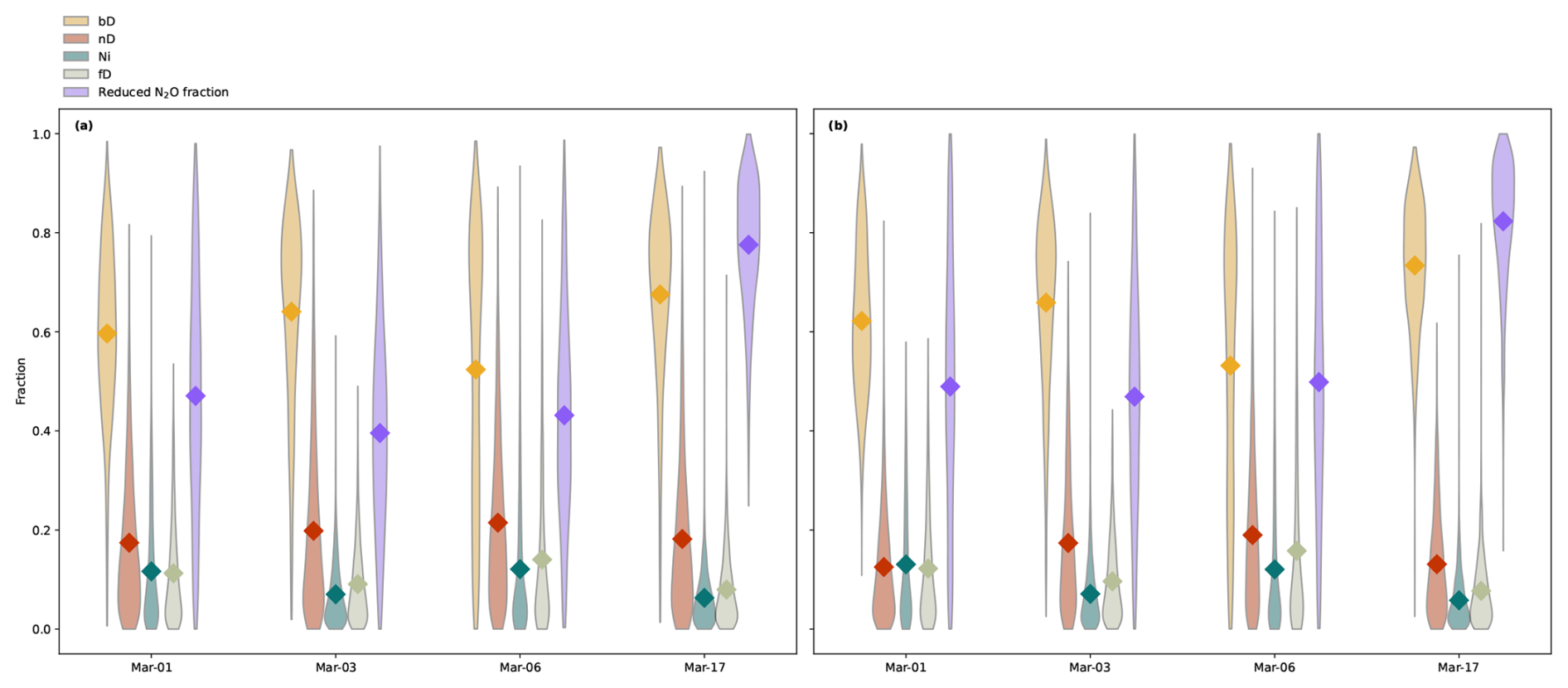
Figure A6 N₂O source fractions and reduced N₂O fraction in March 2023 following fertilization (27–28 February) estimated by the FRAME model. Two alternative model scenarios are shown: (a) mixing-reduction, and (b) reduction-mixing. Violin plots show posterior distributions for heterotrophic bacterial denitrification (bD), nitrifier denitrification (nD), nitrification (Ni), fungal denitrification (fD), and the reduced N₂O fraction. Diamonds indicate mean values.