
the Creative Commons Attribution 4.0 License.
the Creative Commons Attribution 4.0 License.
 | 16 Oct 2026
Tracking crop evapotranspiration and water stress across seasons using multi-sensor UAV observations
Jordan Steven Bates

Harry Vereecken
François Jonard
Accurate estimation of crop evapotranspiration (ET) requires resolving how canopy structure and physiological activity regulate land–atmosphere energy exchange. This study applies the Priestley–Taylor Two-Source Energy Balance (TSEB-PT) model using very-high-resolution UAV multi-sensor observations (∼ 15 cm) to estimate ET over a 10 ha field across three seasons (sugar beet, potato, winter wheat). Thermal infrared data provided land surface temperature (LST), while multispectral (MS) and LiDAR data were used to characterize canopy properties, including a fusion-based estimate of the fraction of LAI that is green (fg) from MS-derived green area index (GAI) and LiDAR-derived plant area index (PAI). Results showed strong sensitivity to LST, highlighting the importance of thermal calibration, and demonstrated that while GAI and PAI performed similarly during peak growth, GAI better captured functional decline during stress and senescence, particularly in dense canopies. Incorporating dynamic fg improved ET estimates across crops and conditions. Modeled instantaneous ET showed good agreement with eddy covariance (EC) measurements, with RMSE ranging from 0.08 mm h−1 to 0.31 mm h−1 and R2 values from 0.28 to 0.97 (highest performance excluding senescence). High-resolution UAV-derived LST data and TSEB-PT modeling also enabled early detection of spatial stress patterns not captured by UAV structural or spectral metrics alone. Upscaling instantaneous ET using a reference ET fraction approach produced daily ET estimates with RMSE ranging from 0.96 to 2.30 mm d−1 and R2 ranging from 0.27 to 0.80 across crops, with improved consistency under energy-balance–closed EC conditions. These daily estimates also enabled assessment of potential crop water stress when compared relative to atmospheric demand (ETRAD= ET ET0) and improved delineation of sub-field variability compared to coarser-resolution methods. These findings demonstrate the value of integrating UAV multi-sensor data with TSEB-PT for robust, high-resolution ET monitoring and practical applications in precision irrigation and water management.
- Article
(17861 KB) - Full-text XML
- BibTeX
- EndNote


Evapotranspiration (ET), the combined loss of water through soil evaporation and plant transpiration, is the second-largest flux in the hydrological cycle after precipitation (Allen et al., 1998). ET plays a critical role in water resource allocation and irrigation scheduling (Wang et al., 2014). Plant health and biomass production is closely linked to transpiration, which depends on soil water availability and is regulated by stomatal and environmental conditions. Accurate, timely estimation of ET at the field scale is essential for optimizing irrigation schedules, improving water use efficiency (WUE) (Pereira and Pires, 2011), and supporting sustainable agriculture amid increasing water scarcity and climate variability (Colaizzi, 2016).
Conventional ET measurement methods, such as lysimeters, sap flow sensors, and eddy covariance (EC) systems (Yang, 2019), offer high temporal resolution but are limited in spatial coverage, making them inadequate for capturing within-field variability critical to precision irrigation (Yao et al., 2017). Additionally, these systems are costly, making large-scale monitoring impractical (Yao et al., 2017). Satellite and airborne remote sensing approaches improve spatial coverage but often lack the resolution needed for dynamic crop monitoring. Manned aircraft, while capable of very-high-resolution observations, are costly and operationally demanding (Bellvert et al., 2020; Hunt and Daughtry, 2018).
Recent advances in unmanned aerial vehicles (UAV) and lightweight, very-high-resolution uncooled thermal infrared (TIR) sensors now enable on-demand, field-scale ET monitoring. UAV platforms offer both high spatial and temporal resolution, allowing for detailed detection of crop water stress and rapid changes in canopy function (Niu et al., 2020). TIR remote sensing in the 8–14 µm range is a key component of energy balance models, as land surface temperature (LST) serves as a direct proxy for canopy transpiration and stomatal regulation if crop aerodynamics are known (Tanner, 1963). Anderson et al. (2024) further reviewed the development of TIR based energy balance models, which link vertical temperature gradients to sensible heat flux by modeling resistance, surface, and vegetation interactions.
Popular and widely used models such as SEBAL and METRIC estimate ET using TIR derived LST and LAI data (Mohan et al., 2020), but their one-source energy balance formulations treat the land surface as a single layer. They rely on hot/cold (not transpiring/fully transpiring) anchor pixels to infer ET extremes, with no explicit representation of soil–canopy interactions or functional canopy condition. This oversimplification can lead to inaccuracies (Niu et al., 2020), especially in heterogeneous or partially senescent fields, where vegetation structure and function vary spatially. However, even though these models are typically used with satellite based remote sensing, they have also been applied with UAV studies (Chandel et al., 2020; Mokhtari et al., 2021; Niu et al., 2019). Some UAV based studies have applied simplified alternatives such as the Deriving Atmosphere Turbulent Transport Useful To Dummies Using Temperature (DATTUTDUT) (Ellsäßer et al., 2020) or the Simple Algorithm for Evapotranspiration Retrieving (SAFER) (de Lima et al., 2024) but have similar constraints for very-high-resolution data at field scale.
Alternatively, Two-Source Energy Balance (TSEB) models partition energy fluxes between soil and vegetation, each with distinct resistances (Norman et al., 1995). It is considered one of the most robust and widely used approaches (Nieto et al., 2022; Nassar et al., 2020), often outperforming OSEB models such as SEBAL or METRIC (Guzinski et al., 2020; Brenner et al., 2018; Jaafar et al., 2022; Tao et al., 2024; Xia et al., 2016), especially in variable and sparse vegetation cover (García-Santos et al., 2022; Derardja et al., 2024). Although TSEB was originally developed for satellite observations representing spatially integrated land–atmosphere exchanges, recent studies have demonstrated that high-resolution UAV data can improve model input characterization (Jaafar and Sujud, 2025) by reducing mixed soil and vegetation signals and better resolving within-field heterogeneity, a primary source of uncertainty at coarser spatial resolutions (Hoffmann et al., 2016; Nassar et al., 2020). Multi-scale analyses further show that pixel mixing strongly influences model performance, as aerodynamic and radiative properties become increasingly spatially averaged at larger grid sizes (Burchard-Levine et al., 2021). There are several versions but the most commonly used is the Priestley–Taylor version (TSEB-PT) (Colaizzi et al., 2014; Yang et al., 2018). Additionally, TSEB-PT incorporates the fraction of LAI that is green (fg) within the Priestley-Taylor formulation which allows the model to dynamically scale transpiration based on the fraction of functioning canopy. This makes it especially suitable for modeling at high spatial resolution with heterogeneous canopy covers from partial stress and senescence conditions. Furthermore, the TSEB-PT version avoids uncertainties tied to vapor pressure compared to the Penman–Monteith (TSEB-PM) version, simplifying deployment for UAV-based applications (Colaizzi et al., 2014). The TSEB model has been used with several UAV crop studies including wheat (Gómez-Candón et al., 2021), barley (Hoffmann et al., 2016), sorghum (Tunca, 2023), and pomegranate (Niu et al., 2019), though many applications focus on vineyards (Gao et al., 2021, 2023; Nassar et al., 2020, 2021, 2022; Nieto et al., 2019; Ortiz et al., 2019; Xia et al., 2016). While the TSEB-2T version has been often used in high-resolution and sparse canopies, like vineyards, where soil and canopy temperatures can be separated. However, its performance has shown mixed results and may decline with increasing canopy closure (Kool et al., 2021; Gao et al., 2023). This is largely due to uncertainties in temperature separation under dense, structurally complex canopies. In contrast, TSEB-PT avoids explicit temperature separation and likely provides more stable performance across varying canopy conditions, suggesting it may be better suited for crops with dynamic vegetation–soil fractions
Recently, machine learning (ML) methods have been applied to ET estimation using multispectral, thermal, and auxiliary data (Amani and Shafizadeh-Moghadam, 2023; Liyew et al., 2025). ML models often depend on large, high-quality ground data such as lysimeters (Kavya and Mahadevaiah, 2024) or eddy covariance systems (Liu et al., 2021), resources that are expensive, sparse, and highly site-specific, limiting their scalability for field-scale operational use (Hirschi et al., 2017) and are time consuming (García-Santos et al., 2022). Moreover, ML models struggle to transfer accurately to different locations or crop systems (Shi and Cai, 2025). In contrast, physically based models such as TSEB-PT provide robust, interpretable, and transferable ET estimates because they are grounded in physically constrained land–atmosphere interactions rather than site-specific training data. The increasing availability of UAV-based multi-sensor observations further enhances these approaches by enabling more detailed characterization of canopy structure, temperature, and surface conditions, opening new opportunities for high-resolution process-based monitoring of crop water use.
Building on these developments, UAV platforms now provide an opportunity to combine physically based energy balance modeling with detailed observations of canopy structure and surface temperature at field scale. In this study we apply the TSEB-PT model for robust, multi-season UAV based ET estimation using very-high-resolution thermal infrared (TIR), multispectral (MS), and LiDAR data. However, small-uncooled TIR sensors are prone to radiometric drift and environmental noise, often requiring ground references to correct LST biases (Kelly et al., 2019). Modeling canopy resistance also hinges on reliable LAI estimates. MS derived green area index (GAI), which reflects pigment concentration, is widely used but susceptible to saturation in dense canopies (Bukowiecki et al., 2020; Zheng and Moskal, 2009). Furthermore, spectral observations primarily characterize green vegetation, while senescent or non-photosynthetic vegetation can remain an important component of total canopy structure (Amin et al., 2021). In contrast, LiDAR is increasingly being used for crop LAI type estimations (Bates et al., 2021; Hütt et al., 2022; Dreier et al., 2025). LiDAR derived plant area index (PAI) captures structural canopy density and reduces saturation-related errors (Bates et al., 2021; Ma et al., 2015). The fraction of LAI that is green (fg), an indicator of photosynthetically active canopy, is rarely used in UAV based TSEB-PT studies. When included, it is typically assumed spatially constant (Hoffmann et al., 2016) or derived from sparse ground samples (Li et al., 2019) or NDVI based estimates, which lack structural depth (Nassar et al., 2022; Mendiguren et al., 2017). In this study, we leverage the complementary strengths of MS (GAI) and LiDAR (PAI) to generate dynamic, spatially explicit fg estimates at pixel level. This has the potential to improve transpiration modeling that accounts for both canopy structure and physiological function.
Our study expands UAV-based TSEB-PT applications across three crop types, sugar beet, potato, and winter wheat, spanning full growing seasons and validated against eddy covariance (EC) measurements. In particular, combining multispectral and LiDAR observations enables independent characterization of canopy physiological condition and structural density, providing a framework to evaluate how functional and structural canopy information influence energy balance partitioning within TSEB. Beyond model validation, we examine the model's ability to capture field-scale evapotranspiration variability and detect early signals of water stress. Specifically, we assess the sensitivity of ET estimates to thermal calibration, compare GAI and PAI as alternative LAI inputs, and evaluate the impact of incorporating fg derived from MS–LiDAR fusion. By testing these components under operational UAV conditions, this work advances the application of TSEB-PT toward high-resolution, process-based monitoring of crop water use using UAV observations.
2.1 Study area
The study was conducted at the ICOS Class 1 ecosystem site DE-RuS within the TERENO Eifel Rur observatory in Selhausen, Germany (50°51′56′′ N, 6°27′03′′ E) (https://ddp.tereno.net/ddp/, last access: 12 October 2026). The 10 ha field is situated at 101–103 m above mean sea level with the soil consisting of Pleistocene loess, Holocene translocated loess, with sand and gravel at deeper levels (Brogi et al., 2020). The western section has shallower sand and gravel deposits, creating spatial variability in crop growth, especially during water-scarce periods. Weather conditions including precipitation and air temperature, during the experiment periods can be found in the appendix (see Table D1 and Fig. D6).
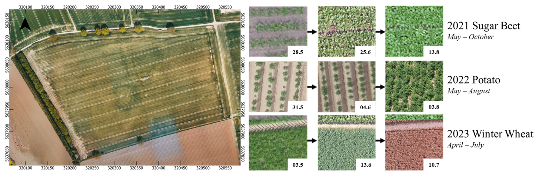
Figure 1The field experiment site (left) with the EC and meteorological station located in the center of the field. The different crop cover type for each year (right) with example images of plant structure and fraction of vegetation coverage over the field throughout each growing season.
The field experiment site, shown in Fig. 1, was monitored over three growing seasons with different crops each year. In 2021, sugar beet was planted from May to October, starting with 20 % vegetation cover and reaching 98 % by harvest. In 2022, potatoes were grown from May to August, beginning with 5 % cover and closing at 87 %, with ridges between rows. In 2023, winter wheat was planted from April to July, maintaining 94 %–98 % cover, with senescence marked by visible leaf browning. Only the potato crop was irrigated, receiving three 30 mm applications in July. These crop and soil variations provide a basis to evaluate the robustness of very-high-resolution UAV data in ET models like TSEB-PT.
2.2 UAV measurements and processing
Two DJI Matrice 600 UAV were used, one carrying a LiDAR payload and the other a combined MS and TIR setup (Fig. 2). The LiDAR system included a YellowScan Surveyor with a Velodyne VLP-16 scanner and Applanix APX15 GNSS-IMU, capturing 300 000 pulses s−1 at 903 nm with ∼ 4 cm precision. Flights were conducted at 50 m altitude and 8 m s−1 with 50 % side overlap. A Septentrio Altus NR3 GNSS base station was used for georeferencing. LiDAR data were processed using POSPac (v8.6) and YellowScan's CloudStation.
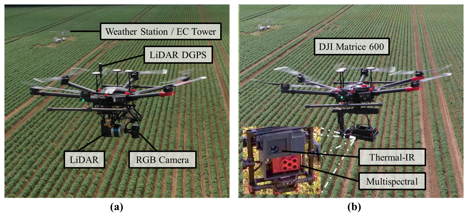
Figure 2View of the DJI Matrice 600 UAV platforms that were used while flying over the field experiment site. (a) The M600 mounted with the YellowScan LiDAR Surveyor and DJI Zenmuse X1 RGB sensor. (b) The M600 with the FLIR Vue Pro R thermal IR modified with a ThermalCapture external heated shutter and Micasense Red-edge M multispectral sensors mounted on a 3-axis gyro system for nadir imagery.
The TIR sensor, a FLIR Vue Pro R 640 (13 mm), covered the 7.5–13.5 µm range with ±5 °C accuracy and was modified with a heated shutter (ThermalCapture, AirRobot® GmbH & Co.) for improved inflight calibration. The MS sensor, a MicaSense RedEdge-M (AgEagle Aerial Systems Inc.), captured five spectral bands; red (663–673 nm) and NIR (820–860 nm) bands were used to calculate NDVI. Both sensors were mounted on a 3-axis gimbal and flown at 100 m altitude and 6 m s−1, with approximately 90 % image overlap. TIR calibration used internal corrections and ground temperature reference targets, while MS data were calibrated using a reflectance panel. Data from both platforms were processed in Pix4D. Flight campaign details are in the Appendix (Table D1).
2.3 UAV data products and model implementation
TSEB-PT inputs were grouped into two categories: (1) surface boundary conditions derived from UAV data, including land surface temperature (LST), fractional cover (fc), leaf area index (LAI), crop height (hc), and fraction of LAI that is green (fg); and (2) meteorological forcing variables, including air temperature (Ta), wind speed (u), vapor pressure (ea), and incoming shortwave irradiance (Sdn). UAV-derived variables were processed and calibrated using ground measurements, with detailed methods provided in Sect. 2.3.1–2.3.5. Data processing and raster analysis were conducted in R using the raster and lidR packages, and all datasets were resampled to a common 15 cm ground sampling distance (GSD). The overall workflow is illustrated in Fig. 3.
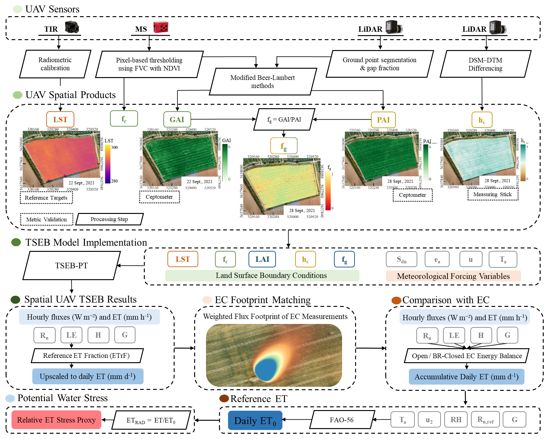
Figure 3Workflow of the study showing UAV and eddy covariance (EC) data integration and TSEB-PT implementation. UAV-derived LST (original vs. corrected), LAI (LiDAR-derived PAI vs. MS-derived GAI), and fg (default = 1 vs. GAI PAI) were varied across model runs. EC-station meteorological forcing for TSEB-PT included incoming shortwave radiation (Sdn), vapor pressure (ea), wind speed (u), and air temperature (Ta). Spatial TSEB-PT outputs were weighted using the modeled EC flux footprint and compared with open and Bowen-ratio (BR)-closed EC observations. Instantaneous ET was upscaled to daily ET using the reference ET fraction (ETrF). Daily reference ET (ET0) was calculated using FAO-56 from Ta, 2 m wind speed (u2), relative humidity (RH), reference-surface net radiation (Rn,ref) and ground heat flux (G), with ET ET0 used as a relative ET stress proxy.
Model runs were designed to assess the impact of key inputs, including LST (original vs. corrected), LAI (MS-derived GAI vs. LiDAR-derived PAI), and fg (default fg=1 vs. UAV-derived fg= GAI PAI), on instantaneous fluxes and ET derived from UAV observations. These outputs were compared with eddy covariance (EC) fluxes and ET within the modeled EC footprint. The analysis was conducted sequentially by first evaluating LST configurations, followed by comparisons of LAI inputs (GAI vs. PAI) with fg held constant (fg=1), and finally incorporating dynamic fg (GAI PAI) with PAI as the structural LAI input.
Following identification of the optimal configuration, instantaneous UAV-based ET estimates were upscaled to daily ET using the reference ET fraction (ETrF) approach and compared with daily EC ET. Reference ET (ET0) was calculated using the FAO-56 method with EC meteorological data to represent atmospheric evaporative demand and was used to derive a relative ET stress proxy (ETRAD) from both UAV- and EC-derived ET estimates.
2.3.1 Land surface temperature (LST) maps
To convert incoming longwave radiance from the TIR microbolometer sensor into land surface temperature (LST), surface emissivity and atmospheric correction parameters were required. Prior to each flight, radiometric calibration parameters, including emissivity, object distance (flight altitude), air temperature, and relative humidity, were updated in the FLIR Vue Pro R camera settings using in-field measurements. These parameters are incorporated within the camera's internal radiometric processing to correct apparent surface temperature for emissivity and atmospheric attenuation effects. Previous studies have demonstrated that LST retrieval from small UAV uncooled sensor microbolometers is highly sensitive to these inputs and requires careful calibration (Kelly et al., 2019; Han et al., 2020; Virtue et al., 2021). Constant emissivity values were assigned to each crop type based on literature, and differences between vegetation and bare soil emissivity were considered negligible due to the limited extent of soil exposure.
Uncooled thermal sensors on UAV platforms, such as the FLIR Vue Pro R, are prone to radiometric instability, largely due to inconsistencies in the internal non-uniformity correction (NUC) applied to the microbolometer focal plane array. To improve calibration consistency, an external heated shutter was employed, which has been shown to substantially improve temperature measurement stability (Virtue et al., 2021). Additional radiometric uncertainty may arise from sensor self-heating and environmental interactions, as temperature drift in uncooled microbolometer arrays can degrade non-uniformity correction and lead to substantial increases in fixed pattern noise, in some cases up to fourfold (Budzier and Gerlach, 2015; Gogler et al., 2014; Sagan et al., 2019). Wind exposure can further destabilize sensor readings (Kelly et al., 2019). To mitigate these effects, the thermal sensor was housed within a custom 3D-printed enclosure providing thermal insulation and wind shielding, and flights were conducted at reduced speeds to minimize wind-induced temperature fluctuations.
Following radiometric correction and sensor stabilization, LST accuracy was evaluated using ground-based reference targets during the 2021 field season. Two reference targets were deployed for each flight: (1) a high-emissivity metallic “hot” plate and (2) a “cold” water target. Target temperatures were measured at the beginning and end of each flight using calibrated contact thermometry (a contact probe attached to the back of the metal plate and an immersion probe for the water container). These measurements were treated as reference temperatures and compared with radiometric temperatures extracted from the UAV thermal imagery over the same targets (Fig. D2).
Despite applying radiometric correction parameters within the camera, a systematic temperature offset remained and varied with meteorological conditions. Consistent with previous findings for uncooled UAV thermal sensors, this residual bias is linked to environmental forcing (Kelly et al., 2019; Han et al., 2020; Virtue et al., 2021). Therefore, a multiple linear regression model was developed using the 2021 reference dataset to relate temperature offsets to air temperature, wind speed, and relative humidity measured at the site. The fitted regression model was subsequently applied to later campaigns (2022–2023) to estimate and correct LST offsets without requiring repeated deployment of reference targets. Two LST inputs were ultimately used in the TSEB model, the original temperature (OG), based solely on the internal radiometric calibration of the sensor, and (2) the target-corrected temperature (TC), which incorporates the regression-based offset correction derived from reference target measurements.
2.3.2 Leaf area index (LAI)
Two representations of canopy density were evaluated as LAI inputs for the TSEB-PT model: multispectral (MS)–derived green area index (GAI) and LiDAR-derived plant area index (PAI). GAI is derived from spectral reflectance and represents the photosynthetically active (green) component of the canopy (Park et al., 2021; Wei et al., 2023), whereas PAI is derived from LiDAR returns and represents total canopy structure independent of pigment content (Bates et al., 2021). Prior to senescence, both metrics act as effective proxies for LAI, as canopy density derived from LiDAR (PAI) and greenness from multispectral indices co-vary with vegetation development and soil–vegetation contrast, until peak growth when structural persistence diverges from declining leaf pigment content (Bates et al., 2021).
GAI and PAI were estimated using modified Beer–Lambert formulations describing radiation attenuation within plant canopies (Ali et al., 2015; Tan et al., 2020; Thorp et al., 2010). GAI was derived from multispectral fractional vegetation cover (FVC), calculated from NDVI using a pixel-based thresholding approach (Jia et al., 2017; Yue et al., 2021; Zhang et al., 2019), while PAI was derived from LiDAR gap fraction (GF), defined as the proportion of laser pulses reaching the ground relative to total returns within each raster cell. In this framework, FVC served both as an intermediate remote-sensing variable for estimating GAI and as the fractional cover (fc) input to pyTSEB for sugar beet and potato, which exhibited partial canopy cover, particularly during early development.
The extinction coefficient (k) was calibrated using in-field SunScan ceptometer LAI measurements (Oguntunde et al., 2012) and applied inversely to estimate GAI and PAI (Eqs. B2–B4). Given the limited number of ground samples per date (four control zones), this semi-empirical approach provided a balance between physical realism and available validation data. Because canopy architecture changes rapidly during early development, 2–3 seasonal k values were assigned per growing season following recommendations of Brogi et al. (2020) and Bates et al. (2021). After canopy closure, k was held constant through peak growth and harvest.
2.3.3 Fraction of LAI that is green (fg)
To separate canopy structure from physiological activity, the fg was computed by combining GAI and PAI. The parameter fg represents the fraction of total canopy structure that remains green and is used within TSEB-PT to scale potential canopy transpiration.
where is the LiDAR scan angle, and kmax is the extinction coefficient derived under peak canopy conditions. This formulation allows fg to dynamically capture divergence between pigment-based canopy function and structural canopy persistence during stress or senescence.
Before senescence, fg was set to 1, assuming a fully functional canopy. After senescence onset, fg decreased according to relative differences between GAI and PAI, allowing transpiration potential to scale with canopy physiological status. Senescence timing was identified using field observations supported by seasonal GAI trends. Sugar beet senescence began in mid-August 2021, potato in early August 2022, and winter wheat in mid-July 2023. For sugar beet and potato, fg was applied following the cessation of ground-based LAI measurements at the onset of senescence. In winter wheat, however, early canopy browning showed substantial spatial variability, particularly in the western portion of the field, before senescence became evident around the central ICOS measurement area. Accordingly, fg was applied from 3 May, preceding the cessation of ground LAI measurements, to capture spatial changes in the fraction of LAI that was green prior to and during senescence.
2.3.4 Fractional cover (fc)
The fc characterizes the horizontal distribution of vegetation and contributes to the representation of canopy spatial heterogeneity and clumping within TSEB-PT (Norman et al., 1995; Kustas and Norman, 1999). For the sugar beet and potato growing seasons, multispectral NDVI-derived fractional vegetation cover (FVC), as described in Sect. 2.3.2, was used as the spatially varying fc input to account for partial canopy cover, particularly during early development. For winter wheat, canopy cover remained nearly complete throughout the UAV observation period (94 %–98 %), and fc was therefore retained at the pyTSEB default value of 1.0.
Within pyTSEB, the supplied fc contributes together with LAI to the representation of canopy clumping and the directional vegetation fraction used for soil–canopy radiometric temperature decomposition (Eqs. A10 and A13–A14). This allows horizontal canopy cover to be represented separately from canopy density and physiological status. Accordingly, structural PAI was used as the LAI input when implementing fg, while fg independently represented the green fraction of LAI contributing to canopy transpiration.
2.3.5 Crop height (hc)
The hc, also referred to as the canopy height model (CHM), was derived using a difference of digital elevation models (DoD) approach (Eq. B5, Appendix B). A pre-emergence UAV LiDAR flight was conducted to obtain a bare-soil digital terrain model (DTM0). Subsequent flight campaigns captured crop surface structure and were used to generate date-specific digital surface models (DSMd). The hc was calculated as the difference between DTM0 and DSMd for each campaign. Using a dedicated bare-soil terrain model rather than ground returns extracted from individual campaigns reduces interpolation uncertainty and improves height accuracy, particularly under dense canopy conditions (Cao et al., 2019). For each raster cell, hc was defined as the maximum canopy elevation above the terrain surface following subtraction of DTM0 from DSMd.
2.3.6 TSEB-PT model and contributions of UAV Derived Inputs
The TSEB-PT model partitions net radiation (Rn) into latent (LE), sensible (H), and ground (G) heat fluxes, with LE converted to evapotranspiration (ET). The model was implemented using the pyTSEB library (Nieto et al., 2018). UAV-derived inputs described in Sect. 2.3.1–2.3.5 constrain key components of the energy balance by influencing radiative partitioning, aerodynamic exchange, and canopy transpiration processes. Figure 4 and Table 1 summarize how each variable contributes to surface–atmosphere interactions within TSEB-PT. Model equations are detailed in Eqs. (A1)–(A15) in Appendix A and Norman et al. (1995).
Table 1UAV-derived model inputs, their roles and interactions within TSEB-PT, and the corresponding equations in which they are used. Equations are provided in Appendix A and the model framework is illustrated in Fig. 4.
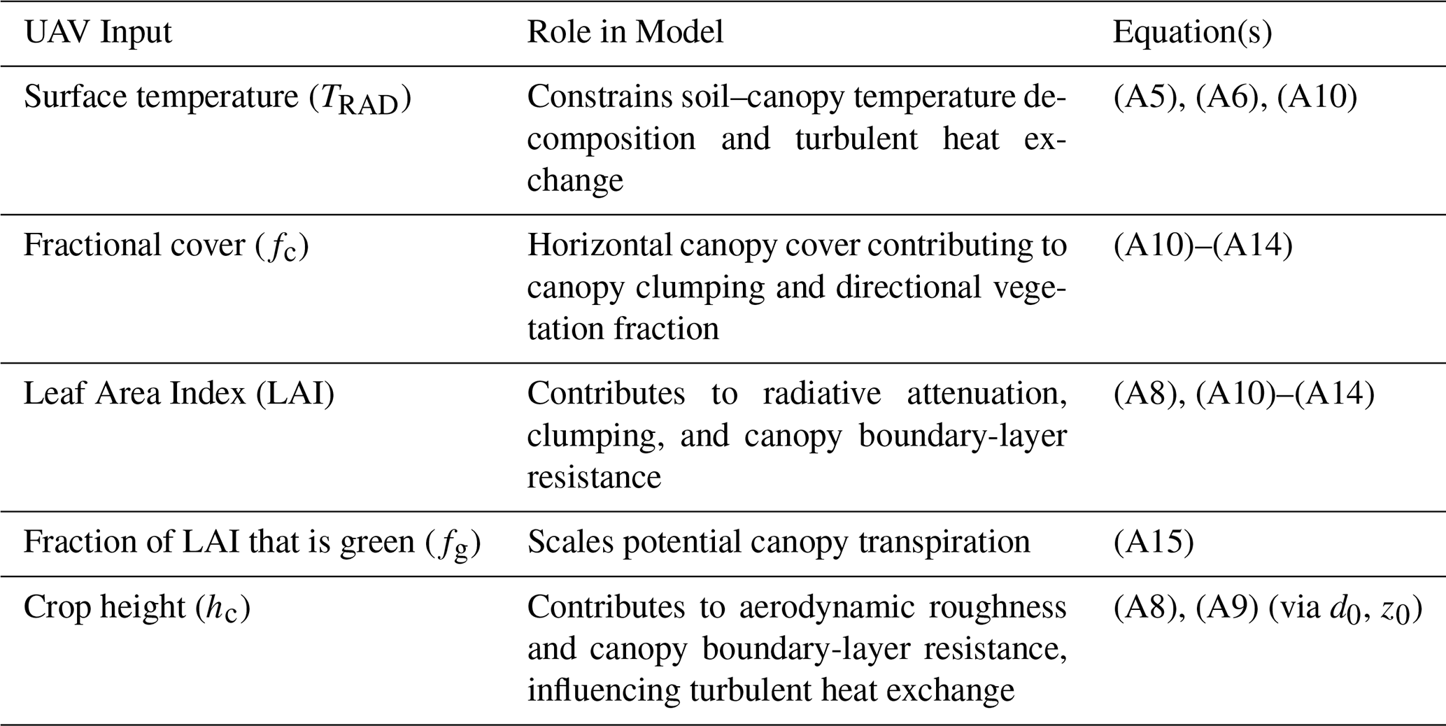
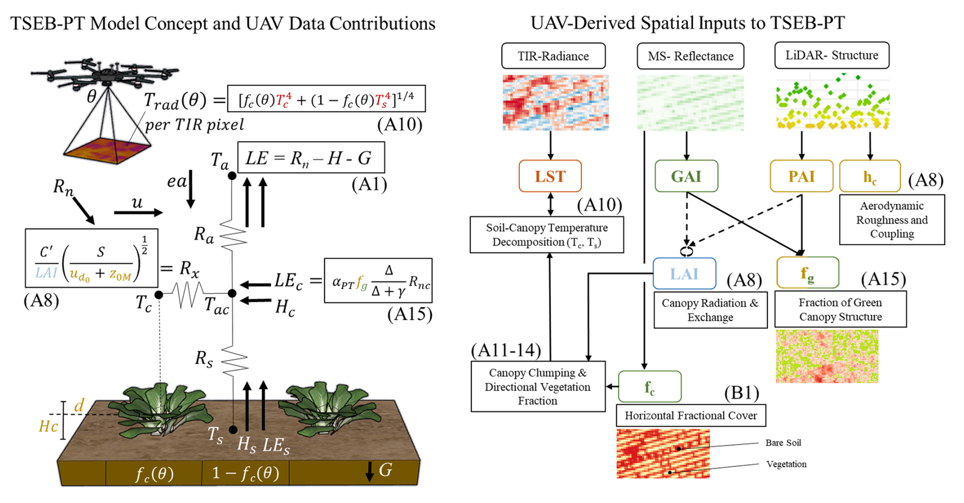
Figure 4Conceptual schematic and example data illustrating how UAV-derived inputs constrain energy-balance partitioning within the TSEB-PT model. The left panel shows the model architecture, highlighting the partitioning of net radiation (Rn) into latent (LE), sensible (H), and ground (G) heat fluxes and the pathways through which UAV-derived variables influence these components. Key inputs include land surface temperature (LST), leaf area index (LAI), fractional cover (fc), fraction of LAI that is green (fg), and canopy height (hc). The right panel illustrates the corresponding UAV-derived spatial inputs and their roles within pyTSEB. Spatially varying multispectral NDVI-derived fractional cover was supplied as the fc input for sugar beet and potato, whereas fc=1 was used for the nearly closed winter wheat canopy. Within pyTSEB, LAI and fc contribute to canopy clumping and the directional vegetation fraction fc (θ) used for soil–canopy radiometric temperature decomposition. The fg scales potential canopy transpiration within the Priestley–Taylor formulation, while LiDAR-derived hc contributes to aerodynamic roughness and turbulent heat exchange. Example spatial data are shown for sugar beet. Abbreviations: Ra (s m−1), aerodynamic resistance to heat transport; Rx (s m−1), canopy boundary-layer resistance; Rs (s m−1), soil boundary-layer resistance; Tc and Ts (K), canopy and soil component temperatures; z0M (m), aerodynamic roughness length for momentum; d0 (m), zero-plane displacement height; and αPT (–), Priestley–Taylor coefficient.
LST provides the radiometric temperature constraint used to resolve soil and canopy temperatures, which in turn strongly influence sensible heat flux through the soil–canopy–atmosphere resistance network. TSEB-PT then partitions available energy between canopy and soil latent and sensible heat fluxes, with potential canopy transpiration initially constrained by the Priestley–Taylor formulation. Consequently, changes in LST can strongly influence energy partitioning and modeled ET. LAI, represented here by either multispectral-derived GAI or LiDAR-derived PAI, influences canopy radiative attenuation, clumping, and canopy boundary-layer resistance (Rx). Increasing LAI generally enhances canopy interception of radiation and reduces the relative contribution of the soil to the surface energy balance. The fc provides complementary information on horizontal canopy distribution and contributes, together with LAI, to canopy clumping and the directional vegetation fraction used for soil–canopy radiometric temperature decomposition (Eqs. A10–A14). The fg regulates canopy transpiration within the Priestley–Taylor formulation. In model runs incorporating fg, reductions in fg decrease canopy latent heat flux without altering the prescribed structural LAI or fractional-cover inputs, allowing ET to decline during stress or senescence even when canopy structure remains dense. This distinction is particularly important in dense canopies, where reduced transpiration may otherwise be masked by structural cooling effects (Elfarkh et al., 2020; Kustas et al., 2016). The hc affects aerodynamic roughness length () and displacement height (d), thereby influencing aerodynamic resistance and turbulent heat exchange between the surface and atmosphere. Together, these inputs enable TSEB-PT to separately represent structural controls on radiation exchange and physiological controls on transpiration, improving interpretation of spatial and seasonal variability in ET.
2.3.7 Weather station, EC ET, and flux footprints validations
Ground measurements were collected to support UAV data validation and model calibration. Eddy covariance (EC) flux data, processed according to ICOS standards, were used to evaluate UAV-derived evapotranspiration (ET) estimates (Schmidt et al., 2025a, b). EC measurements of wind speed, wind direction, and water vapor concentration were used to compute vertical turbulent fluxes associated with ET (Ghiat et al., 2021).
The spatial representativeness of EC observations was addressed through flux footprint modelling. Flux footprints were estimated using the flux footprint prediction (FPP) model implemented in R (Kljun et al., 2015), which accounts for micrometeorological conditions and surface roughness characteristics. Footprints were calculated for the duration of each UAV flight, and UAV-based TSEB-PT ET estimates were compared with EC measurements by extracting weighted averages of raster pixels within the 90 % cumulative footprint extent. Individual footprint examples are provided in Appendix D (Fig. D1). This approach reduces scale mismatch between point-based EC observations and spatially distributed UAV flux estimates by accounting for the dynamic source area contributing to measured turbulent fluxes.
Energy balance closure was addressed using the Bowen-ratio-preserving correction of Twine et al. (2000), consistent with previous UAV-based TSEB studies (e.g., Hoffmann et al., 2016; Brenner et al., 2017, 2018; Gao et al., 2023). Model evaluation primarily relied on comparisons with open EC fluxes to avoid introducing additional assumptions related to closure corrections (Mokhtari et al., 2021; Nassar et al., 2021). Nevertheless, comparisons using energy-balance-closed fluxes are also presented to assess the sensitivity of model performance to EC energy balance correction.
3.1 UAV data derived model inputs
UAV thermal infrared (TIR) observations consistently underestimated ground-surface temperature relative to in-field reference targets during 2021. Uncorrected TIR data had an RMSE of 4.19 °C but maintained strong temporal agreement across dates (R2= 0.97). Ground-target correction reduced the seasonal RMSE to 2.78 °C. Thermal error was most strongly associated with air temperature (r=0.74), followed by wind speed (r=0.55) and relative humidity (r=0.34). These relationships were used in a multiple linear regression model to correct sensor bias in subsequent seasons, producing an average LST increase of 2.2 °C across acquisitions. Correction relationships and validation are presented in Fig. D2, while seasonal differences between original (LSTOG) and corrected (LSTTC) field-average LST are shown in Fig. 5.
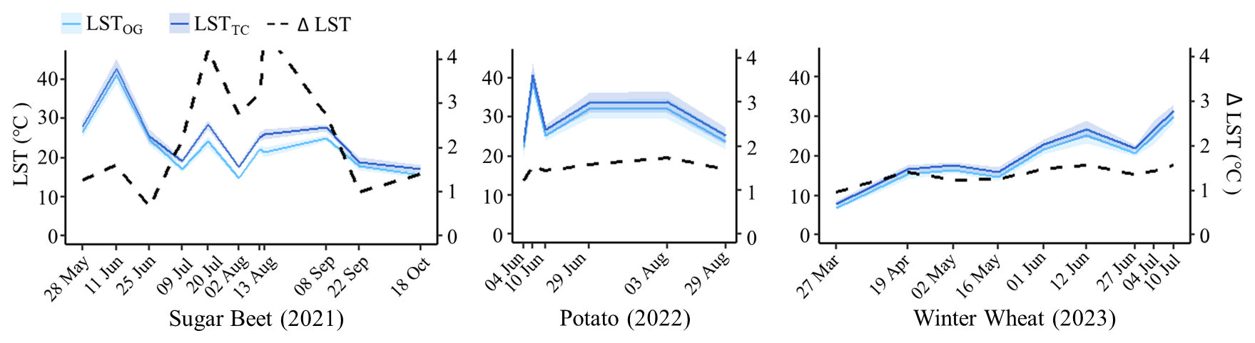
Figure 5Field-averaged land surface temperature (LST) before (LSTOG) and after temperature correction (LSTTC). The dashed line represents the temperature difference between the two LST estimates.
Multispectral-derived green area index (GAI) and LiDAR-derived plant area index (PAI) were evaluated against ground-based ceptometer LAI measurements (Fig. 6). PAI showed closer agreement with ground observations across crops, with R2=0.99 and an overall RMSE of 0.27 m2 m−2, compared with R2=0.88 and RMSE =1.02 m2 m−2 for GAI, based on a limited number of calibration samples. Differences between GAI and PAI were greatest during senescence, when GAI declined while LiDAR-derived PAI retained higher canopy structural values.
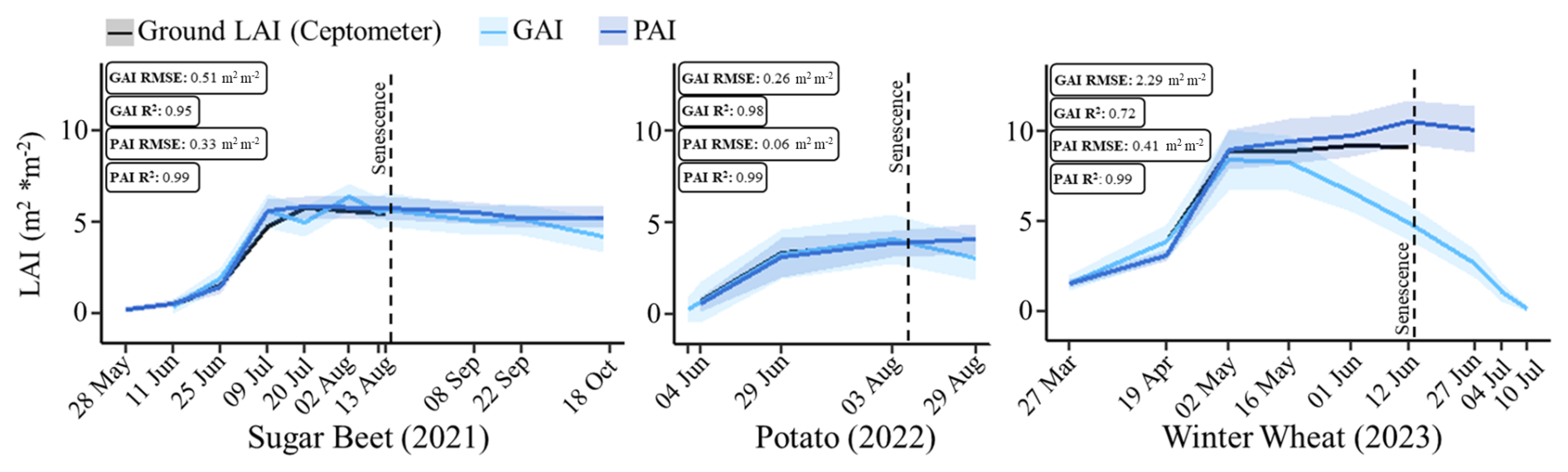
Figure 6Field averaged UAV derived green area index (GAI) and plant area index (PAI) compared to ground based ceptometer LAI measurements across each campaign for three growing seasons. Ground measurements conclude prior to the onset of senescence, during which divergence between GAI and PAI becomes more pronounced due to declining pigment content in the canopy.
UAV-derived canopy height (hc) also showed strong agreement with ground measurements (Fig. 7), with an overall RMSE of 0.06 m and R2=0.90 across crops. Winter wheat showed the highest agreement (RMSE =0.01 m; R2=0.99), while potato showed greater error (RMSE = 0.12 m), potentially reflecting ridge planting and heterogeneous canopy closure within sampled areas.
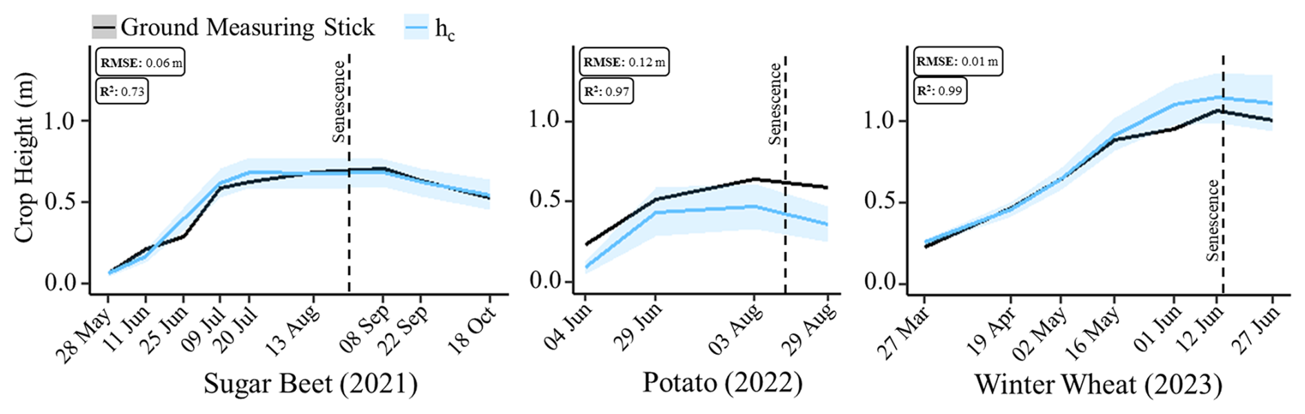
Figure 7Comparison of UAV LiDAR derived canopy height (hc) and ground based measuring stick data for each season. UAV derived values represent field wide averages, while ground measurements reflect averages within designated control point (CP) zones.
3.2 Accuracy and sensitivity of TSEB-PT ET estimates from UAV thermal corrections
To assess the impact of radiometric calibration on model performance, TSEB-PT estimates derived from original (LSTOG) and target-corrected (LSTTC) UAV thermal imagery were compared with EC fluxes under open and closed energy balance conditions across all three crop seasons (Fig. 8). Thermal correction generally produced slightly lower modeled net radiation (Rn) and latent heat flux (LE) and higher sensible heat flux (H), with the largest responses in sugar beet (2021) and winter wheat (2023) and more moderate changes in potato (2022). Soil heat flux (G) changed comparatively little. Overall, LSTTC improved agreement with EC observations, particularly for LE and under closed energy balance conditions.
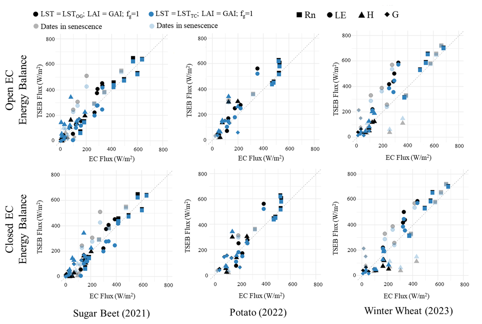
Figure 8Comparison of modeled TSEB-PT energy fluxes (Rn, LE, H, and G) with eddy covariance (EC) observations across three crop seasons. Upper panels show comparisons using open EC energy balance fluxes, while lower panels show closed EC energy balance fluxes. Colors indicate land surface temperature inputs (original, LSTOG; target-corrected, LSTTC), symbols indicate flux components, and shaded points represent observations acquired during senescence.
RMSE and R2 statistics (Table D2) supported these patterns. Thermal correction generally reduced LE RMSE across crops, with the largest improvements for winter wheat and sugar beet, whereas responses in H were less consistent. Rn showed minimal sensitivity and G generally exhibited smaller and crop-dependent responses. Excluding senescence dates strengthened agreement, particularly for LE. Across configurations, closed EC energy balance comparisons generally produced higher R2 and lower RMSE than open EC comparisons.
Because LE represents evapotranspiration within the energy balance, estimates were converted to ET (mm h−1) for direct evaluation at UAV acquisition times (Fig. 9). Under open EC conditions, LSTTC reduced RMSE from 0.21 to 0.16 mm h−1 for sugar beet, 0.14 to 0.11 mm h−1 for potato, and 0.31 to 0.26 mm h−1 for winter wheat. Thermal correction did not always improve temporal correspondence; for sugar beet, R2 decreased from 0.50 to 0.32 despite the lower RMSE. Excluding senescence dates further strengthened agreement, with the largest improvement in sugar beet (RMSE 0.16 to 0.11 mm h−1; R2 0.32 to 0.79). Closed EC comparisons generally produced higher R2 and slightly lower RMSE across crops.
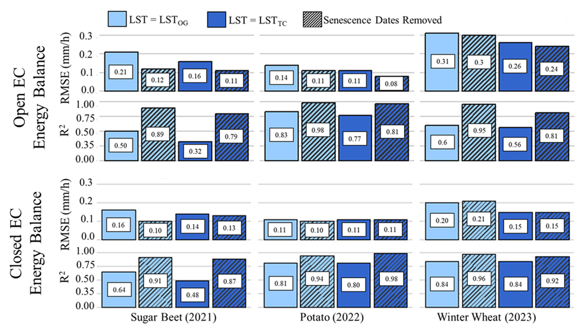
Figure 9RMSE and R2 between modeled TSEB-PT ET and EC-derived ET under open and closed energy balance conditions, averaged over the EC flux footprint. Model runs are compared using original (LSTOG) and target corrected (LSTTC) land surface temperature inputs. Metrics are shown for the full growing season and with senescence periods excluded.
3.3 Accuracy and sensitivity of TSEB-PT ET estimations from different UAV based LAI inputs
Building on the thermal correction analysis, we evaluated the influence of multispectral-derived GAI, LiDAR-derived PAI, and dynamic fraction of LAI that is green (fg= GAI PAI) on TSEB-PT flux estimates (Fig. 10; Table D3). Differences between GAI and PAI configurations were generally small during early- to mid-season conditions when canopy structure and greenness were closely aligned, with similar agreement with EC observations under both open and closed energy balance comparisons.
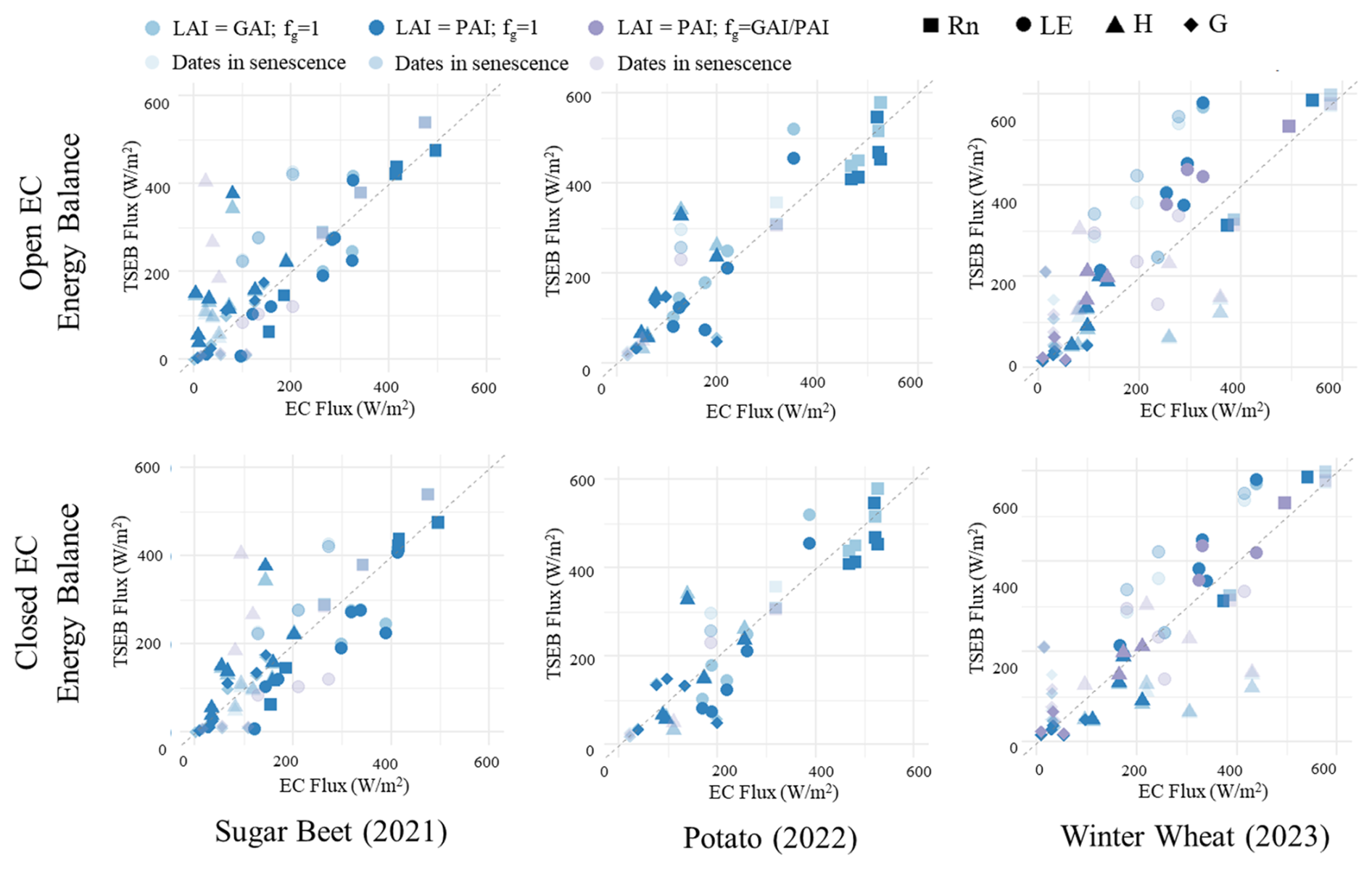
Figure 10Comparison of modeled TSEB-PT energy fluxes (Rn, LE, H, and G) with eddy covariance (EC) observations across three crop seasons under different LAI and fg parameterizations. Upper panels show comparisons using open EC fluxes, and lower panels show closed EC energy balance fluxes. Colors indicate model configurations (GAI; PAI; PAI with dynamic (fg), symbols indicate flux components, and lighter markers represent senescence-period observations.
Differences became more pronounced during senescence, particularly in winter wheat. Using PAI with fg=1 resulted in greater LE overestimation, whereas GAI improved agreement with EC observations. Using PAI together with dynamic fg further reduced this bias and shifted modeled fluxes closer to the 1:1 relationship (Fig. 10; Table D3). Similar but smaller responses were observed for sugar beet and potato. Across crops, LAI configuration had comparatively small effects on Rn and G, while LE and H showed greater sensitivity. Closed EC comparisons generally produced higher R2 and lower RMSE than open EC comparisons.
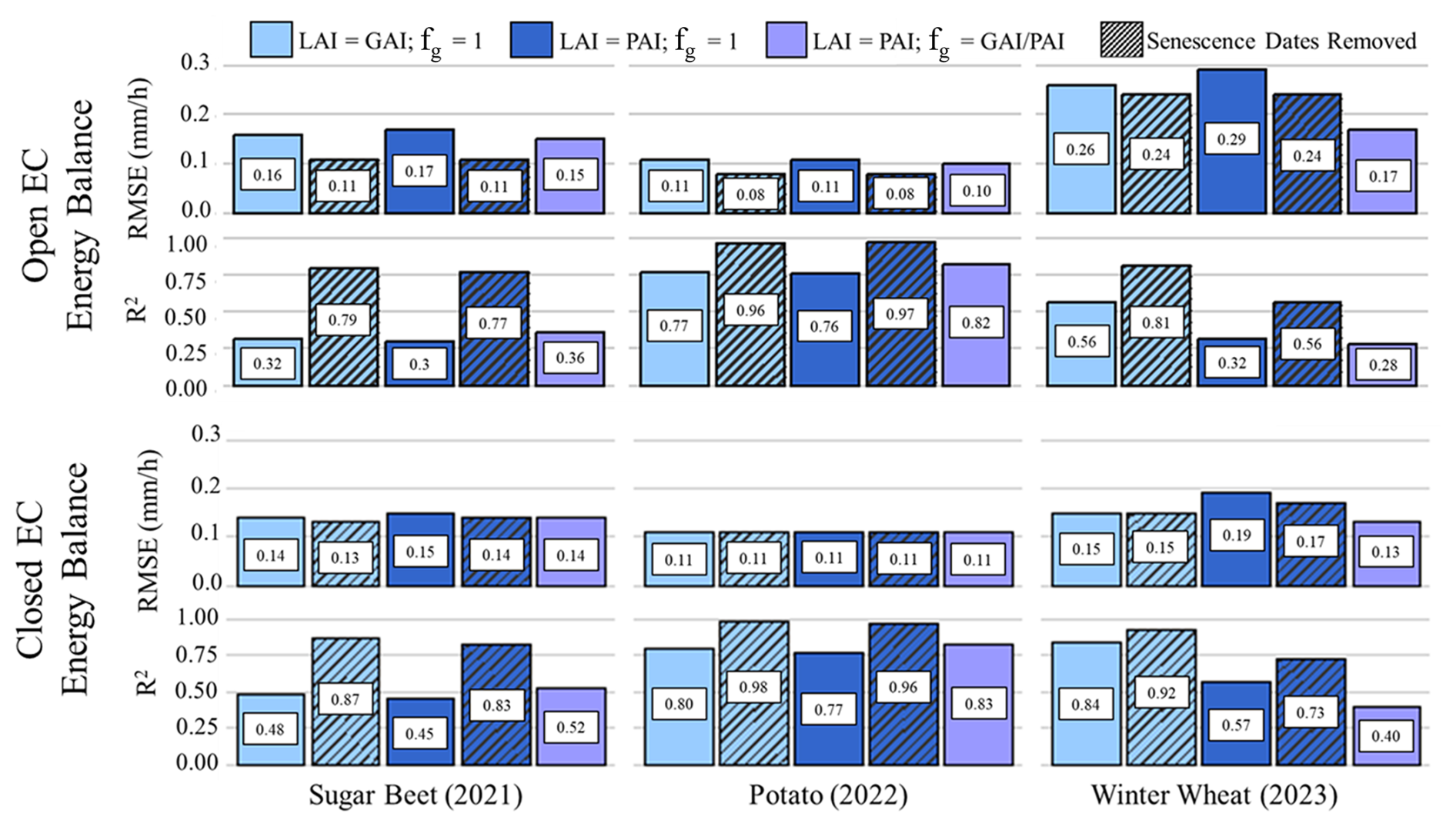
Figure 11RMSE and R2 between TSEB-PT modeled ET and EC-derived ET under open and closed energy balance conditions, averaged over the EC flux footprint. Green area index (GAI) and plant area index (PAI) were evaluated as LAI inputs for all campaign dates and with senescence dates excluded. A third configuration using PAI with spatially dynamic fg was evaluated during senescence to account for changes in green canopy fraction.
ET comparisons further demonstrated these differences (Fig. 11). For winter wheat, under open EC energy balance conditions, PAI with fg=1 produced greater ET overestimation (RMSE ≈ 0.29 mm h−1; R2 ≈ 0.32) than GAI (RMSE ≈ 0.26 mm h−1; R2 ≈ 0.56), while incorporating dynamic fg, with LAI = PAI, reduced RMSE to approximately 0.17 mm h−1 and improved agreement. Across crops, comparisons with closed EC ET generally showed similar or improved performance based on R2 and RMSE. Excluding senescence dates reduced differences among LAI configurations across all crops, with differences between GAI and PAI becoming minimal, indicating similar performance before senescence.
3.4 Input impacts on ET magnitude and spatial variability
TSEB-PT ET varied in both magnitude and spatial distribution depending on the UAV-derived inputs. To assess their influence on spatial variability, changes in the coefficient of variation (CV) of ET were compared with differences in input CV for LST (TIROG vs. TIRTC), LAI (GAI vs. PAI), and fg (fg=1 vs. GAI PAI-derived fg) (Fig. D4). LST correction produced substantial changes in ET spatial variability despite the largely uniform temperature offset, while differences between GAI and PAI had a comparatively smaller influence. In contrast, dynamic fg substantially altered ET spatial variability, demonstrating a stronger influence on the spatial representation of ET than LAI source alone.
The spatial effects of LST correction were further examined for potato under early- and late-season canopy conditions (Fig. D5). During early development, when fractional cover was lower, LST correction increased spatial contrasts associated with soil and vegetation contributions to ET. Later in the season, ET reductions following LST correction were greater in areas exhibiting vegetation stress, increasing the contrast between stressed and non-stressed zones. Thus, thermal correction affected not only ET magnitude but also the spatial representation of modeled crop water use.
3.5 Precise early identification of crop water stress with high-res ET maps
One of the most practical advantages of TIR based UAV derived ET modeling is its capacity to detect early signals of crop water stress before structural or spectral changes manifest in traditional vegetation indices. In the 2022 potato and 2023 winter wheat seasons, this capability was clearly demonstrated as seen in Figs. 12 and 13.
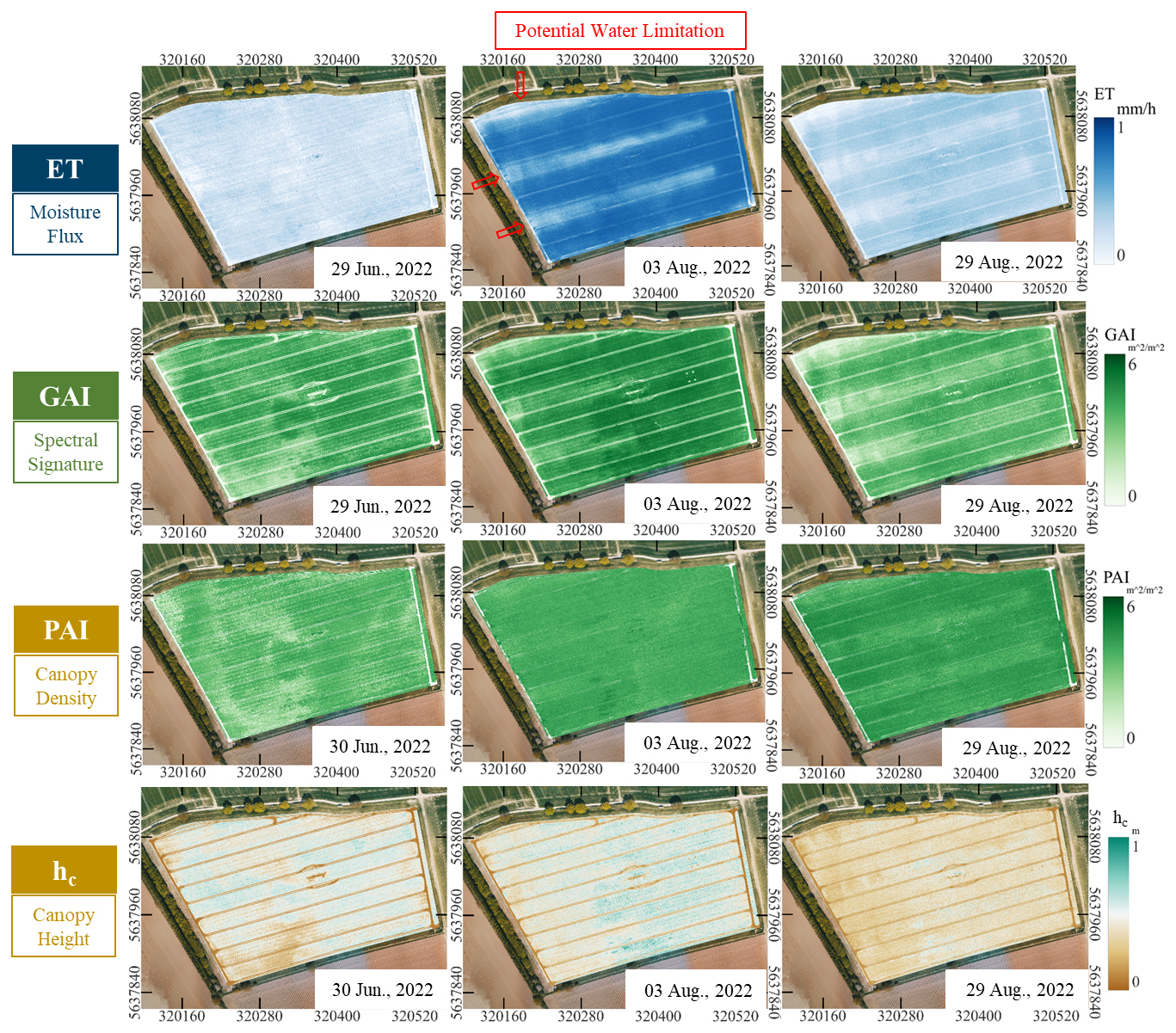
Figure 12Evapotranspiration (ET), green area index (GAI), plant area index (PAI), and crop height (hc) during selected dates of the 2022 potato season illustrating the development of potential water stress. On 3 August, distinct within-field patterns associated with irrigation are evident in ET, while remaining less apparent in GAI, PAI, and hc. By 29 August, similar patterns are also evident in GAI, PAI, and hc, indicating subsequent changes in canopy greenness and structure.
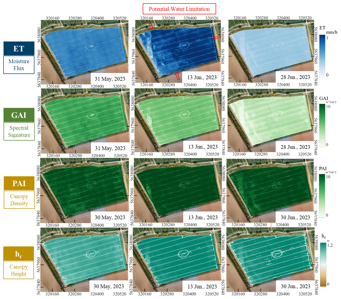
Figure 13Evapotranspiration (ET), green area index (GAI), plant area index (PAI), and crop height (hc) during selected dates of the 2023 winter wheat season illustrating the development of potential water stress. Before stress onset, no pronounced spatial patterns are evident. On the second date, distinct within-field patterns emerge in ET, while remaining less apparent in GAI, PAI, and hc. By the final date, similar patterns are also evident in GAI, PAI, and hc, indicating subsequent changes in canopy greenness and structure. These patterns are consistent with differences in soil properties and rooting depth across the field.
Comparisons between the 3 and 29 August UAV campaigns in 2022 revealed that, despite minimal changes in both GAI and PAI, the ET maps captured pronounced declines in water use across specific sections of the field. These reductions aligned with known zones of reduced irrigation coverage caused by limitations of the hose reel sprinkler system. Notably, areas along the northwest corner and adjacent to irrigation lanes exhibited significant ET suppression, even though they remained structurally intact in LiDAR and multispectral imagery.
A similar pattern was observed in 2023 with winter wheat, though in this case the stress was most likely attributed to known underlying soil–root interactions that have caused water stress in the past. On 13 June, the ET map revealed broader and more pronounced spatial structures of suppressed transpiration that were not yet visible in the GAI or PAI maps. By 28 June, however, similar spatial patterns emerged in both GAI and PAI, confirming physiological and structural canopy decline.
3.6 Upscaling Instantaneous UAV ET to Daily Values for Agricultural Water Management
To evaluate the operational applicability of UAV-derived ET, instantaneous estimates were upscaled to daily values using the reference ET fraction (ETrF) approach and compared with daily EC ET under open and closed energy balance conditions and with FAO-56 reference ET (ETo) (Allen et al., 1998; Appendix Sect. C3). Upscaling followed Cammalleri et al. (2014) using the best-performing TSEB-PT configuration (LST = LSTTC, LAI = PAI, fg= GAI PAI, and LiDAR-derived hc). A relative ET stress proxy (ETRAD = ET ETo ) was calculated to characterize crop water use relative to atmospheric evaporative demand.
Figure 14 presents daily EC ET, ETo, and upscaled UAV ET aggregated over the field, EC flux footprint, and potential water-limitation zones (PWLZ; Figs. 12–13). UAV-derived daily ET generally followed the temporal patterns of EC ET and ETo across crops, while PWLZ estimates frequently differed from field and footprint averages. Correspondingly, ETRAD declined below 0.7 and 0.5 during several periods, particularly within PWLZs, indicating progressively greater reductions in ET relative to atmospheric demand.
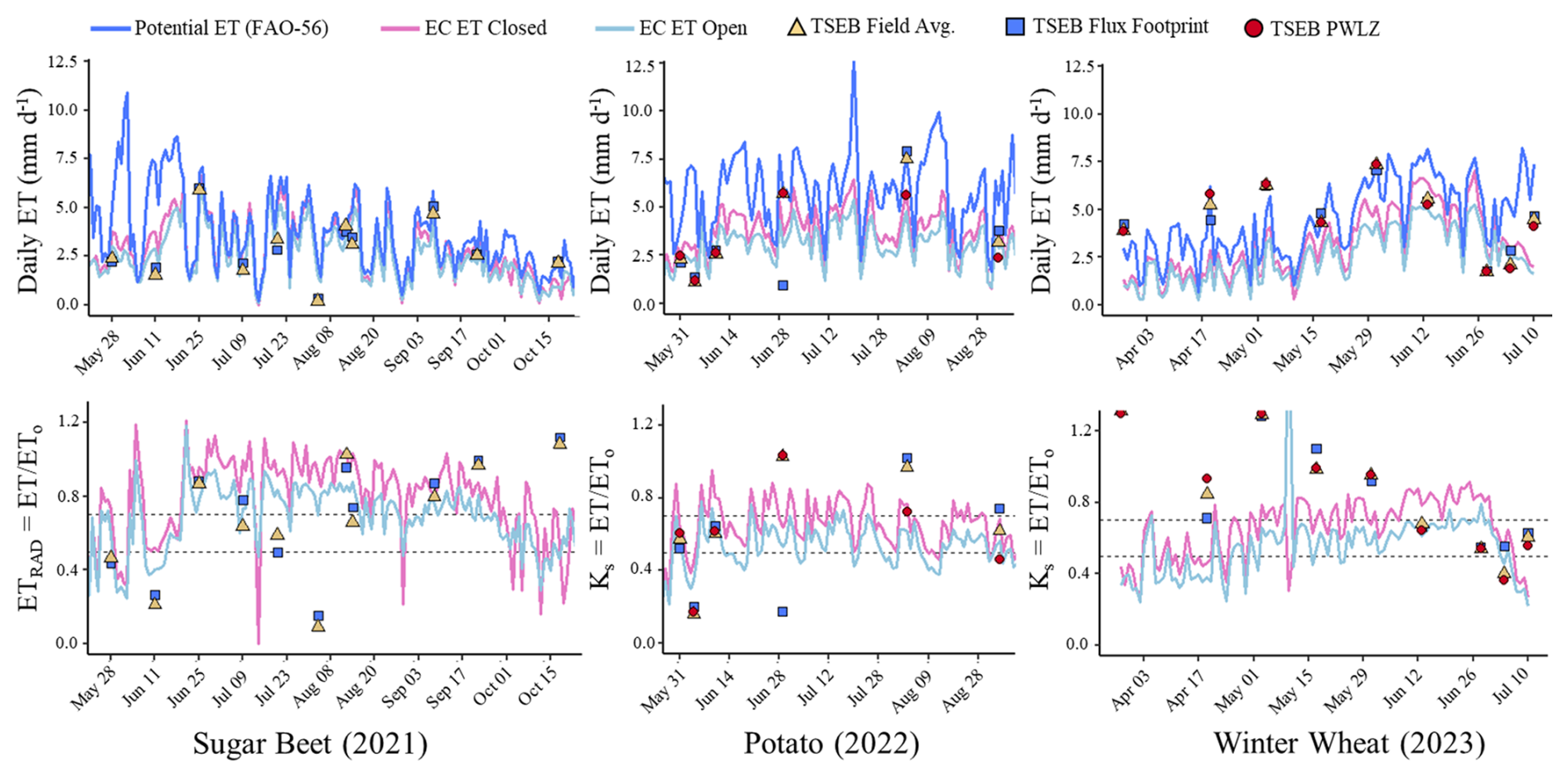
Figure 14Daily evapotranspiration (ET) time series and relative ET stress proxy derived from UAV–TSEB and EC measurements. Top panels show upscaled UAV ET compared with daily EC ET (open and closed energy balance) and FAO-56 reference ET (ETo). Bottom panels show the relative ET stress proxy (ETRAD = ET ETo). Dashed lines indicate ETRAD thresholds of 0.7 and 0.5, representing progressively greater reductions in ET relative to atmospheric evaporative demand. Symbols distinguish UAV ET aggregated over the field, EC flux footprint, and potential water-limitation zones (PWLZ; Figs. 12–13).
Daily UAV-derived ET performance against EC observations is summarized in Fig. 15. Agreement varied among crops and EC energy balance treatments. Sugar beet showed moderate agreement (RMSE = 0.96–1.30 mm d−1; R2=0.57–0.61), while potato showed the strongest agreement (RMSE = 1.53–1.61 mm d−1; R2 ≈ 0.80). Winter wheat showed the weakest agreement (RMSE = 1.90–2.30 mm d−1; R2=0.27–0.30).
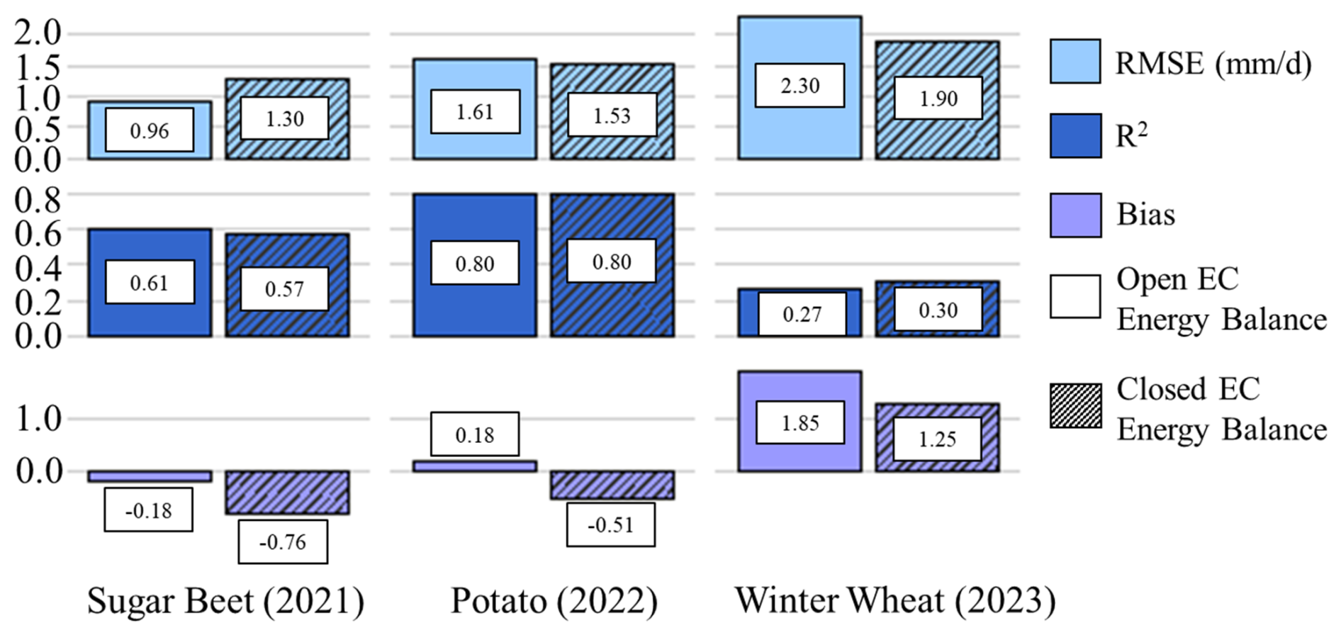
Figure 15Comparison of daily UAV-derived TSEB ET against EC measurements for sugar beet (2021), potato (2022), and winter wheat (2023). Performance is evaluated using RMSE (mm d−1), R2, and bias (mm d−1) under open and closed EC energy balance conditions. Closed EC estimates are shown with hatched bars.
Bias was also crop dependent, ranging from −0.18 to −0.76 mm d−1 for sugar beet, +0.18 to −0.51 mm d−1 for potato, and +1.25 to +1.85 mm d−1 for winter wheat. Differences between open and closed EC comparisons demonstrate the influence of energy balance treatment on model evaluation and the uncertainty associated with EC-derived ET as a reference.
4.1 Thermal accuracy and impacts on spatial ET distribution
TSEB-PT's strong sensitivity to land surface temperature (LST) is well established (e.g., Hoffmann et al., 2016), but this study extends those findings using very-high-resolution UAV based thermal imagery under uniform crop cover. Uncorrected LST exhibited a significant underestimation, consistent with prior UAV studies (e.g., Kelly et al., 2019; Han et al., 2020; Wan et al., 2024; Tunca et al., 2023; Liu et al., 2024). This bias led to systematic ET overestimation. While R2 declined slightly after correction, the improved thermal realism enhanced physical consistency in ET estimates, particularly important for cumulative ET tracking and water balance assessments.
Thermal bias was most severe under high air temperature and wind speed, precisely when crops face peak transpiration demand and are most vulnerable to stress. This trend aligns with Sagan et al. (2019), who reported increased UAV TIR underestimation under warmer conditions. In our results, stressed areas showed amplified ET deviations with LST correction, indicating greater sensitivity to thermal accuracy. Underestimated LST muted ET suppression signals, reducing contrast between stressed and non-stressed zones and potentially misguiding irrigation responses. In addition, corrected LST sharpened spatial gradients in ET by enhancing energy balance contrast, particularly under dominant water or energy limitation conditions. This raised the standard deviation of ET values across the field and improved spatial differentiation of stress signals.
Despite onboard radiometric correction and a heated shutter for non-uniformity calibration, ground based reference targets remained essential for accurate LST and ET retrieval. When such targets are unavailable, alternate approaches like the Dual-Temperature Difference (DTD) variant of TSEB-PT has shown to improve estimations (Hoffmann et al., 2016). Although in our case, DTD yielded only moderate improvements compared to ground-calibrated correction when used for the 2021 campaign (results not shown).
Finally, LST accuracy could be further improved through spatially dynamic emissivity correction. While constant emissivity values are appropriate under full canopy closure during peak growth, they become less valid under partial canopy conditions (e.g., early growth stages in sugar beet and potato) and during senescence, particularly in cereal crops such as winter wheat where strong contrasts between green, functioning vegetation and brown, senescent material introduce greater emissivity variability. Recent work has shown that emissivity can be effectively parameterized using NDVI to distinguish between soil, vegetation, and mixed pixels in high-resolution UAV datasets (e.g., NDVI segmentation or scaling approaches) (Heinemann et al., 2020). Applying such methods could improve LST retrievals in heterogeneous and senescing canopies, thereby enhancing spatial ET estimation and stress detection.
4.2 Implications of LAI and fc source and sensitivity to plant physiological properties
Both GAI and PAI served as effective LAI inputs for TSEB-PT during peak growth, when structural (PAI) and pigment-based (GAI) indicators were closely aligned, yielding similar ET estimates. This is consistent with a prior one-source energy balance study showing that LiDAR-derived LAI can perform comparably to multispectral-derived LAI for ET estimation (Wei et al., 2023). However, few studies have examined how model performance shifts under stress or senescence, when canopy structure and function can diverge.
When fg was held at its default value of 1, PAI remained high due to persistent canopy structure and was associated with greater ET overestimation during these periods. In contrast, GAI declined with senescence and produced more conservative ET estimates that better aligned with EC observations, particularly in winter wheat, where structural density persisted as canopy greenness and transpiration declined. Although PAI and ground-based ceptometer LAI showed better agreement in absolute magnitude, they did not reflect the decline in green canopy area to the same extent as GAI. The improved performance of GAI relative to PAI may therefore indicate that its decline indirectly represented part of the reduction in transpiring green vegetation that was otherwise not accounted for when fg remained at its default value, whereas PAI better retained information on persistent canopy structure.
For sugar beet and potato, spatially varying NDVI-derived fc accounted for partial canopy cover and soil exposure, providing complementary information on the horizontal distribution of vegetation. Together with LAI, fc contributes to canopy clumping and the directional vegetation fraction used to decompose radiometric temperature into soil and canopy component temperatures. These component temperatures influence soil–canopy sensible heat partitioning and, consequently, the energy balance from which G is estimated (Eq. A4 in Appendix A). The crop-specific differences in ground heat flux (Table D2) therefore suggest that the relative performance of GAI and PAI may depend partly on canopy architecture. PAI may have improved G estimates in winter wheat by better representing canopy density and structural shading in the tall, closed canopy, whereas GAI performed better in the lower, more open sugar beet and potato canopies with greater vegetation–soil contrast, suggesting that the relative benefits of multispectral and LiDAR inputs may depend on canopy architecture. However, these interpretations are inferred from the model behavior observed in this study, and targeted sensitivity testing is needed to establish the underlying mechanisms.
4.3 Role of fg in differentiating functional transpiration from passive cooling
Distinguishing passive canopy cooling from actual transpiration is critical in dense canopies like winter wheat, where structure remains even as physiological function declines. Unlike eddy covariance systems, which directly measure vapor flux, TSEB-PT relies on LST as a proxy. Without accounting for canopy function, models may incorrectly attribute radiative cooling to transpiration. In this study, combining LiDAR based structural LAI (PAI) and MS derived pigment-sensitive LAI (GAI) enabled the calculation of a spatially dynamic fg, allowing canopy transpiration within the Priestley–Taylor formulation to be scaled according to physiological status, improving ET agreement with EC observations, particularly during early stress and senescence.
The dynamic fg also improved model performance before pronounced visible senescence, indicating sensitivity to periods when transpiration was suppressed due to stress. Although fg is an available TSEB-PT input, it is frequently omitted and retained at its default value of 1 in applications. Comparable explicit structural–functional scaling is absent from single-source models such as SEBAL and METRIC. More broadly, these approaches were developed primarily for conventional remote-sensing applications, where detailed characterization of canopy structure and function is more limited than with current UAV observations. UAV platforms provide an opportunity to better exploit this distinction by combining high-resolution three-dimensional structural information from LiDAR with spectral information related to canopy greenness.
Previous UAV-based TSEB-PT studies that did not dynamically parameterize fg also reported ET overestimation under conditions of declining canopy function. Gómez-Candón et al. (2021) reported ET overestimation in wheat (RMSE = 0.24 mm h−1), particularly later in the season during senescence. Similarly, Tunca (2023) reported overestimation in stressed sorghum and suggested adjustment of the Priestley–Taylor coefficient (α) as a potential solution. The present results indicate that dynamic fg provides a spatially explicit means of scaling canopy transpiration within the Priestley–Taylor formulation, rather than relyingon a uniform adjustment of αPT. Bozorgi et al. (2024) likewise identified assumptions concerning the fg as a potential source of TSEB bias, further supporting the importance of representing changes in the fraction of LAI that is green.
As shown in Fig. D4, fg influenced spatial ET variability more strongly than LAI type alone, demonstrating the sensitivity of modeled ET to fg and the importance of accurately representing this variable. This sensitivity was greater for sugar beet and potato than for winter wheat. The high LAI of winter wheat may have contributed to its reduced response, as exponential radiation attenuation in dense canopies results in diminishing changes in radiation interception with increasing LAI (Campbell and Norman, 1998; Kustas and Norman, 1999); however, the mechanisms underlying the observed crop-specific sensitivity to fg require further investigation.
UAV LiDAR methods can now provide purely structural, high-resolution information that complements multispectral estimates of canopy function, helping to reduce pigment-related biases inherent in reflectance-only approaches (Chirouze et al., 2014). Unlike maximum NDVI methods, which may not fully capture structural changes during senescence, combining LiDAR-derived structure with MS-based greenness allows fg to better represent the green fraction relative to total canopy structure. This integrated approach can improve ET partitioning and may be beneficial for broader application in UAV-based TSEB-PT and other ET modeling workflows.
4.4 Upscaling instantaneous UAV TSEB to daily ET and performance
To support applications in irrigation management and water balance assessment, instantaneous evapotranspiration (ET) estimates derived from UAV-based TSEB-PT were upscaled to daily totals. TSEB provides flux estimates corresponding to the time of thermal acquisition, requiring temporal upscaling for daily ET estimation. In this study, daily ET was derived using the ETrF approach (Sect. 3.6; Eq. C2) based on the best-performing instantaneous configuration (LST = LSTTC, LAI = PAI, fg= GAI PAI). This approach enabled direct comparison with EC-derived daily ET and with reported daily ET estimates from previous studies.
The resulting daily ET estimates showed good agreement with EC observations across crops, although winter wheat remained the most challenging. Relatively few studies report daily field-scale TSEB performance for the crops examined here, and the available studies are predominantly satellite-based. For winter wheat, reported daily ET RMSE values are approximately 1.5–2.0 mm d−1 (El Hazdour et al., 2025). Other satellite-based energy-balance approaches have reported similar errors; for example, Zoratipour et al. (2023) obtained daily winter wheat ET RMSEs of 2.15 and 1.53 mm d−1 for SEBAL and SEBS, respectively. These comparisons place the present UAV-based TSEB-PT results within the range reported for other remote-sensing ET approaches, while UAV observations provide greater spatial detail and acquisition flexibility. This is consistent with Nassar et al. (2020), who showed that increasing model grid size had a comparatively smaller effect on field-scale mean fluxes than on within-field variability, while Mokhtari et al. (2021) demonstrated the value of higher-resolution UAV data for resolving fine-scale spatial variability in ET. However, direct comparisons between studies should be interpreted cautiously because of differences in spatial and temporal resolution, crop conditions, and validation and EC-processing methods.
Crop-specific behavior further illustrates differences in model performance. Winter wheat showed a tendency toward ET overestimation, consistent with previous studies reporting positive bias under dense canopy conditions (El Hazdour et al., 2025), where structural persistence may lead to overestimation of transpiration when physiological activity declines. In contrast, studies on sugar beet (Acharya and Sharma, 2021) and potato (Ebert et al., 2022) have reported slight underestimation of ET, which may be associated with higher soil exposure during early growth stages. Greater soil exposure increases the contribution of the soil component to radiometric temperature and influences soil–canopy energy partitioning within TSEB (Norman et al., 1995; Kustas and Norman, 1999). Consistent with this interpretation, the largest underestimations in this study occurred during early growth stages of sugar beet and potato, when soil fractions were highest (Fig. 14).
Future improvements in daily ET estimation could involve both alternative upscaling formulations and improved temporal sampling. Evaporative-fraction, radiation-based, and other scaling approaches can exhibit different performance depending on phenology, environmental conditions, and acquisition time (Nassar et al., 2021). Recent developments include improved evaporative-fraction-based temporal scaling (Wei et al., 2025) and machine-learning approaches for instantaneous-to-daily flux upscaling (Tunca, 2026). UAV platforms also provide flexibility in acquisition timing and the potential for repeated observations within a day. Together, these developments suggest that improved daily ET estimation may require a combination of appropriate temporal-scaling methods, optimized acquisition timing, and, where feasible, multi-temporal observations that better characterize the diurnal ET cycle.
4.5 Future considerations with UAV TSEB model implementation
Additional UAV sensor capabilities could further improve TSEB parameterization. Multi-layer LiDAR gap-fraction profiles could improve characterization of vertical canopy structure (Bates et al., 2026b), while LiDAR intensity has shown relationships with crop LAI (Hütt et al., 2022) and biomass (Montzka et al., 2023), potentially extending LiDAR from a purely structural measurement toward a dual-purpose source of structural and intensity-based canopy information. Ground-classified LiDAR observations could also provide information on soil-surface roughness, potentially helping to guide the selection or adjustment of soil roughness and resistance parameters, which have been shown to influence TSEB performance (Li et al., 2019). Additional information on canopy and surface moisture could be provided by emerging UAV radar systems, including synthetic aperture radar (SAR) and ground-penetrating radar (GPR) (Wu and Lambot, 2022), while integration of surface soil moisture has been shown to improve TSEB transpiration estimates (Song et al., 2023). Hyperspectral UAV observations offer another complementary source of physiological information, potentially enabling retrieval of SIF and PRI, with SIF providing information linked to photosynthetic activity and transpiration and PRI providing sensitivity to changes in photosynthetic light-use efficiency and stress responses (Jonard et al., 2020; Zheng et al., 2024). These indicators could help refine fg or support alternative approaches to better represent canopy physiological status in TSEB-PT. Together, these sensors offer opportunities to advance UAV-based ET modeling by integrating complementary information on three-dimensional canopy structure, moisture status, and canopy function.
Another important consideration is the influence of shadowing on remote sensing inputs. Studies have shown that shadow pixels can introduce bias in LST and ET estimation, as shaded surfaces exhibit lower temperatures that may lead to artificially elevated modeled ET under some conditions (Mokhtari et al., 2021). Additional work has demonstrated that shadowing can significantly affect vegetation indices and the retrieval of fc and LAI, thereby providing an additional pathway through which illumination conditions can influence TSEB flux partitioning (Lu et al., 2022; Gao et al., 2023). These effects may be particularly important in discontinuous canopies with greater soil exposure (Duran-Gomez et al., 2026). However, shaded pixels form part of the composite radiometric signal, and their removal may not necessarily improve flux estimation; recent work instead supports approaches that retain or compensate for shadow effects (Aboutalebi et al., 2019; Duran-Gomez et al., 2026). LiDAR-derived structural inputs provide an advantage in this context because they are substantially less dependent on illumination conditions than passive sensor observations. Although shadow effects were likely reduced in this study by near-solar-noon acquisitions and predominantly developed canopies, future UAV-TSEB studies should further evaluate shadow-compensation strategies for both multispectral and thermal inputs.
UAV acquisition flexibility also provides opportunities to improve temporal representation. Flights can be targeted near optimal acquisition periods or repeated throughout the day to characterize diurnal ET variability and changing illumination conditions, including the movement and influence of shadows. This flexibility may also complement satellite observations by supporting temporal interpolation between satellite overpasses (El Hazdour et al., 2025), as well as high-resolution validation and spatial sharpening of satellite-derived products (Jaafar et al., 2022). Combining the spatial detail and acquisition flexibility of UAV observations with the broader spatial and temporal coverage of satellite systems may therefore improve both within-field characterization and temporal continuity of ET estimates.
Finally, further improvements may arise from testing alternative resistance formulations and soil heat flux parameterizations. Modified resistance schemes have improved TSEB performance under particular canopy conditions (Li et al., 2019; Lun et al., 2026), while simplified G parameterizations remain an important source of uncertainty (Hoffmann et al., 2016). In this study, G was sensitive to LAI representation, with GAI performing better in the more open sugar beet and potato canopies and PAI in dense winter wheat, further motivating targeted testing of how UAV-derived structural and spectral canopy information can best parameterize these model inputs. Model configuration may also be adapted to canopy conditions. Preliminary application of TSEB-2T to the 2021 sugar beet campaign (data not shown) indicated improved performance during early development under low vegetation cover, whereas TSEB-PT was more robust under dense canopy conditions. Future work could therefore examine how model configuration, parameterization, and UAV-derived canopy inputs can be adapted according to canopy architecture and phenological stage.
4.6 Practical impacts and considerations for farming practices, water stress, and irrigation
Moving toward practical farm management applications, physically based models such as TSEB-PT offer advantages by explicitly representing land–atmosphere energy exchange without requiring the extensive training datasets typically needed for data-driven approaches such as machine learning. In this study, TSEB-PT provided ET estimates across three crop seasons with relatively limited ground inputs, consisting primarily of a small number of control plots for LAI and canopy height calibration and early-season thermal reference targets. This demonstrates the potential of combining physically based modeling with UAV observations, with complementary sensor information improving characterization of canopy structure, function, and surface temperature.
The high spatial resolution of UAV ET mapping enables detection of sub-field variability that may not be resolved by conventional scouting or coarser satellite observations. In this study, TIR-derived ET revealed crop water stress patterns before corresponding changes became evident in multispectral GAI or LiDAR-derived PAI and hc. In potato, ET maps revealed zones of reduced ET following irrigation events, consistent with under-irrigation (Fig. 12), while persistently low ET in winter wheat corresponded with shallow gravel layers and areas exhibiting potential water stress and earlier senescence (Fig. 13). Such spatial information can help identify zones of contrasting crop water use and support targeted irrigation management.
A daily relative ET stress proxy (ETRAD= ET ET0) was used to characterize crop water use relative to atmospheric demand, consistent with previous approaches (Giardina et al., 2023). Comparisons among field averages, EC footprints, and delineated stress zones (Fig. 14) demonstrate how spatial aggregation can mask localized stress signals, particularly in potato during 3–29 August. However, low ETRAD does not necessarily indicate water limitation, as reduced ET may also reflect other physiological constraints on transpiration. Complementary information, such as in situ or remotely sensed soil moisture, could therefore help attribute ET reductions to water deficit and improve interpretation of ET-based stress signals.
Previous studies similarly support energy-balance approaches for crop water-stress assessment. TSEB-derived transpiration and stomatal conductance have provided robust stress indicators compared with temperature-based indices alone (Nieto et al., 2022), while combining ET-related information with CWSI has improved discrimination of irrigation treatments and water deficits in UAV applications (Sánchez-Virosta et al., 2025). Operationally, UAV-derived ET could be combined with rainfall and irrigation records to estimate spatial crop water deficits and support irrigation scheduling. Additional integration with gross primary productivity (GPP) and water-use efficiency (WUE) could further connect crop water use with productivity (Elfarkh et al., 2023). High-resolution ET information has consequently been identified as valuable for agricultural water management (Wanniarachchi and Sarukkalige, 2022), with UAV-based approaches offering opportunities for spatially targeted interventions (Ankela et al., 2026).
Despite these advantages, operational implementation requires consideration of spatial scale. The 15 cm GSD outputs generated here exceed the resolution typically required for irrigation decisions, which are generally implemented at irrigation-sector or management-zone scales (von Hebel et al., 2021). Such zones can be defined by soil, yield, crop, and ET variability and typically operate at meter- to tens-of-meter scales or as a limited number of homogeneous field units (Serrano et al., 2020; Flint et al., 2023). The principal value of very-high-resolution UAV ET may therefore lie not in managing individual pixels, but in identifying meaningful within-field heterogeneity that can subsequently be aggregated into actionable management zones. This provides a multi-scale framework in which fine-resolution observations support stress detection and characterization, while aggregated information supports irrigation planning and decision-making.
This study demonstrates the potential of integrating very-high-resolution UAV multi-sensor observations with TSEB-PT for field-scale evapotranspiration (ET) estimation across sugar beet, potato, and winter wheat over full growing seasons. With relatively limited ground calibration of UAV inputs, modeled ET showed good agreement with eddy covariance (EC) observations, although performance varied among crops and winter wheat remained the most challenging. Agreement was largely maintained when instantaneous estimates were upscaled to daily ET using a ETrF approach, supporting the application of UAV-based TSEB for crop water-use assessment. Reference ET was further used to contextualize modeled ET relative to atmospheric demand, enabling identification of potential water stress conditions. High-resolution UAV ET maps revealed clear spatial patterns of reduced ET associated with likely water-limited zones, which would not be apparent from coarser-scale observations. Comparisons of stress proxies across spatial scales demonstrated how aggregation to field-average and EC-footprint scales can mask localized reductions in crop water use.
Among the UAV inputs, thermal infrared observations were both highly influential and an important source of uncertainty. The uncooled thermal sensor underestimated LST under high-temperature and high-VPD conditions, contributing to ET overestimation, while ground-based thermal correction improved ET magnitude and spatial representation. Vegetation inputs showed similarly important crop- and phenology-dependent behavior. LiDAR-derived PAI and multispectral-derived GAI performed comparably when canopy structure and greenness were closely aligned, but diverged during stress and senescence as PAI retained persistent canopy structure while GAI declined with green canopy area. Combining these complementary sensitivities through dynamic fg (GAI PAI) substantially improved ET performance, particularly when structural and functional canopy properties diverged.
Overall, the results highlight the value of combining thermal, multispectral, and 3D LiDAR observations rather than relying on a single UAV sensor. The physically based TSEB framework provides a means of integrating these complementary observations while requiring relatively limited ground information and remaining applicable across different crop types. Together with flexible acquisition timing and very-high spatial resolution, this approach provides opportunities for identifying within-field water-use variability and supporting spatially targeted crop-water management.
Key contributions of this study include:
-
Demonstrating the robustness of UAV-based TSEB-PT across three crop types with limited ground calibration, while identifying crop-specific modeling challenges, particularly in dense winter wheat canopies.
-
Underscoring the importance of accurate TIR calibration for ET estimation, particularly under high-temperature conditions.
-
Demonstrating comparable performance of LiDAR-derived PAI and multispectral-derived GAI when canopy structure and greenness were closely aligned, and their divergence during stress and senescence.
-
Proposing a LiDAR–MS fusion approach to derive dynamic fg for transpiration scaling and demonstrating its value for improving ET estimates across changing physiological conditions.
-
Demonstrating the potential of UAV TIR-based ET mapping to detect early patterns of potential water stress before corresponding changes became evident in other sensor-derived canopy metrics, supporting targeted irrigation management.
Future improvements should focus on advancing thermal calibration and dynamic emissivity characterization, improving the representation of LAI, fc, and fg, and further integrating structural and physiological UAV observations. Combining UAV and satellite observations through spatial fusion and temporal interpolation could extend these high-resolution estimates across broader spatial and temporal scales, strengthening their application to crop-water monitoring and irrigation management.
The Two-Source Energy Balance model with Priestley-Taylor formulation (TSEB-PT; Norman et al., 1995) was used to estimate surface energy fluxes, particularly latent heat flux (LE), by partitioning soil and canopy contributions based on radiometric surface temperature. The model was implemented in Python using the open-source pyTSEB package (Nieto et al., 2018). For more detailed description of TSEB, please refer to Norman et al. (1995) and Kustas and Norman (1999).
A1 Energy balance equations
Fluxes are partitioned into canopy and soil components:
Soil heat flux G is parameterized as a fraction of Rns:
where cg=0.35 is an empirical constant (Choudhury et al., 1987; Kustas and Daughtry, 1990).
A2 Sensible heat partitioning and air temperature
The total sensible heat flux H is calculated as:
where Tac= within-canopy air temperature (equivalent to the aerodynamic temperature; Kelvin); Tc and Ts are the canopy and soil component temperatures (K), respectively, resolved from the UAV-observed composite radiometric surface temperature; ρ is the air density (kg m−3); Cp is the specific heat capacity of air at constant pressure (J kg−1 K−1); Ra, Rs, and Rx are the aerodynamic, canopy boundary-layer, and soil boundary-layer resistances to heat transport (s m−1), respectively.
The within-canopy air temperature Tac is defined as:
A3 Resistance parameterizations
Soil boundary layer resistance (Kustas and Norman, 1999):
where us is wind speed immediately above the soil surface (m s−1), Ts−Tac is the soil-to-canopy-air temperature difference (K), and b and c are empirical coefficients of the Kustas and Norman (1999) formulation. Default pyTSEB values were retained.
Canopy boundary-layer resistance (Norman et al., 1995):
LAI is the effective leaf area index supplied to pyTSEB, in this study represented by either UAV multispectral GAI or LiDAR PAI; l (m) is the effective leaf width; is wind speed at the canopy momentum source–sink height (m s−1); The zero-plane displacement height (d0=0.65hc) and aerodynamic roughness length for momentum (z0M=0.125hc) were estimated from UAV-derived crop height (hc). C′ (s m−1) =90 s m−1 is the default empirical coefficient of the Norman et al. (1995) formulation.
where zT is the air-temperature measurement height (m), d0 is the zero-plane displacement height (m), is the aerodynamic roughness length for heat transport (m), u* is friction velocity (m s−1), k=0.41 is the von Kármán constant, L is the Monin–Obukhov length (m), and ΨH is the atmospheric stability correction function for heat transport.
A4 Radiometric temperature decomposition and canopy clumping
The observed directional radiometric temperature (TRAD) is decomposed into canopy (Tc) and soil (Ts) component temperatures according to their relative contributions to the sensor field of view (Norman et al., 1995):
where fc (θ) represents the directional fraction of vegetation observed by the sensor at viewing zenith angle θ, The directional vegetation fraction is estimated as:
where kbe (θ) is the canopy extinction coefficient at viewing zenith angle θ, calculated from the Campbell (1990) leaf-angle distribution as:
where χ is the Campbell (1990) parameter describing the canopy leaf-angle distribution.
For partially covered or spatially heterogeneous canopies, pyTSEB additionally accounts for canopy clumping when estimating the directional vegetation fraction. The nadir clumping index, Ω(0), is estimated from LAI and the supplied fractional-cover input (fc) following Kustas and Norman (1999):
with local LAI (F) defined as:
where LAI is the effective LAI supplied to pyTSEB, fc is the fractional-cover model input, and F represents the local LAI within the vegetated fraction of the surface. In this study, multispectral NDVI-derived FVC was supplied as fc for sugar beet and potato, whereas fc=1 was retained for the nearly closed winter wheat canopy. Thus, the fractional-cover input fc and LAI contribute to the estimation of canopy clumping and, consequently, to the directional vegetation fraction used in Eq. (A10).
For observations acquired at non-zero view zenith angles, pyTSEB can account for the angular dependence of canopy clumping through the directional clumping index Ω(θ). In this study, UAV thermal imagery was acquired with a nadir-oriented gimbal and the sensor view zenith angle was set to θ=0°. Consequently, Ω(0)=Ω0, and the directional vegetation fraction fc(θ) in Eqs. (A10)–(A11) was evaluated at nadir.
A5 Priestley-Taylor approach to canopy transpiration
The initial estimate of LEc uses the Priestley-Taylor formulation:
where αPT=1.26 and is iteratively reduced until a physically plausible solution is obtained (LEs>0) (Kustas and Anderson, 2009); fg is the fraction of LAI that is green; Δ is the slope of the saturation vapor pressure curve (kPa K−1); γ is the psychrometric constant (kPa K−1); and Rnc (W m−2) is canopy net radiation.
B1 Fractional Vegetation Cover and Green area index (multispectral)
with NDVIs is the NDVI value representative of bare soil and NDVIv is the NDVI value representative of full/healthy vegetation.
k(θ)= extinction coefficient, parametrized using SunScan ceptometer LAI measurements. k was adjusted once between early and mid-late season and then held constant through senescence.
B2 Plant area index (LiDAR)
nground= number of LiDAR returns classified as ground. n= total number of returns (ground + vegetation) in the pixel.
LiDAR scan angle; GF = gap fraction from previous equation; k = extinction coefficient (same as above), adjusted once mid-season and then held constant.
B3 Crop height (LiDAR)
DSMd= digital surface model from the crop canopy (per flight date); DTM0= digital terrain model from the bare soil pre-emergence flight.
C1 Eddy Covariance Closure Method – Bowen ratio (BR)–preserving method
For hourly eddy covariance (EC) flux and the accumulative daily ET, a Bowen ratio–preserving approach following Twine et al. (2000) was used for closed energy balance conditions as follows:
C2 FAO 56 reference ET
The reference evapotranspiration (ET0) was calculated using the FAO-56 method (Allen et al., 1998) as follows:
Rn is net radiation at the reference surface (MJ m−2 d−1); G is the soil heat flux density (MJ m−2 d−1); T is mean daily air temperature at 2 m (°C); u2 is wind speed at 2 m (m s−1); es and ea are saturation and actual vapor pressure (kPa); Δ as the slope of the saturation vapor pressure curve (kPa °C−1); and γ as psychrometric constant (kPa °C−1). Reference ET was used to represent atmospheric evaporative demand, for temporal upscaling of instantaneous UAV-derived ET, and for expressing estimated ET relative to atmospheric demand.
C3 TSEB upscaling to daily ET using reference ET fraction (ETrF)
where ETrF is the reference evapotranspiration fraction, ETinst is instantaneous UAV-derived ET, and ET0,inst is reference ET calculated for the corresponding UAV observation period. The instantaneous ETrF was then multiplied by daily reference ET (ET0,daily) as follows:
where ETdaily is the upscaled daily UAV-derived ET. ETrF differs from the evaporative fraction (EF = LE (Rn−G)) and was used for temporal upscaling following Cammalleri et al. (2014).
C4 Relative ET stress proxy
ET estimates from UAV TSEB-PT and EC were expressed relative to atmospheric demand using:
where ET is the estimated evapotranspiration and ET0 is the FAO-56 reference evapotranspiration calculated as described in Sect. C2. ET relative to atmospheric demand (ETRAD) was used as a relative ET stress proxy, with lower values indicating greater suppression of ET under a given atmospheric evaporative demand.
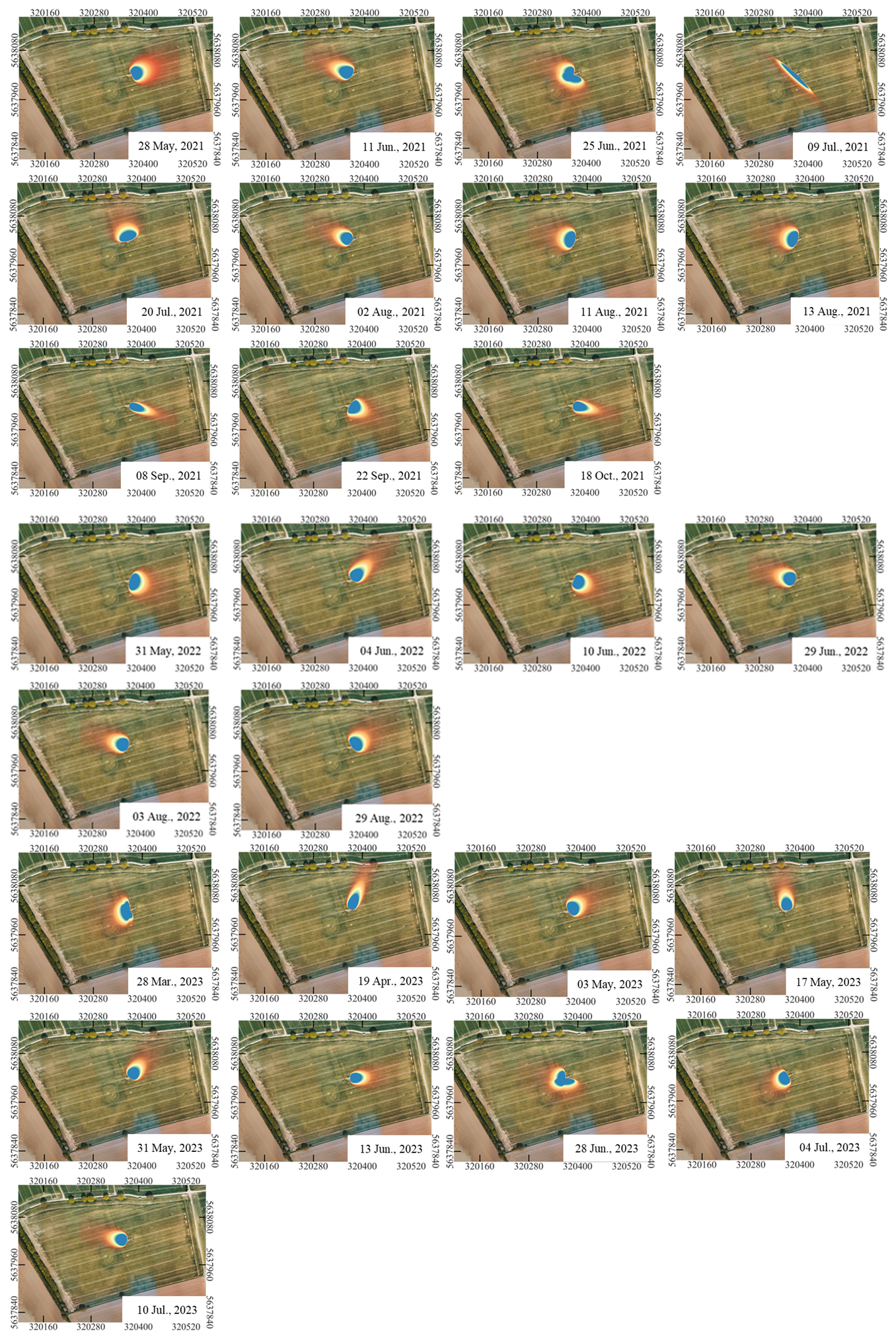
Figure D1The estimated EC footprints for each TIR campaign flight time interval to be used to compare the TSEB-PT ET values within this spatial extent to the EC ET estimations.
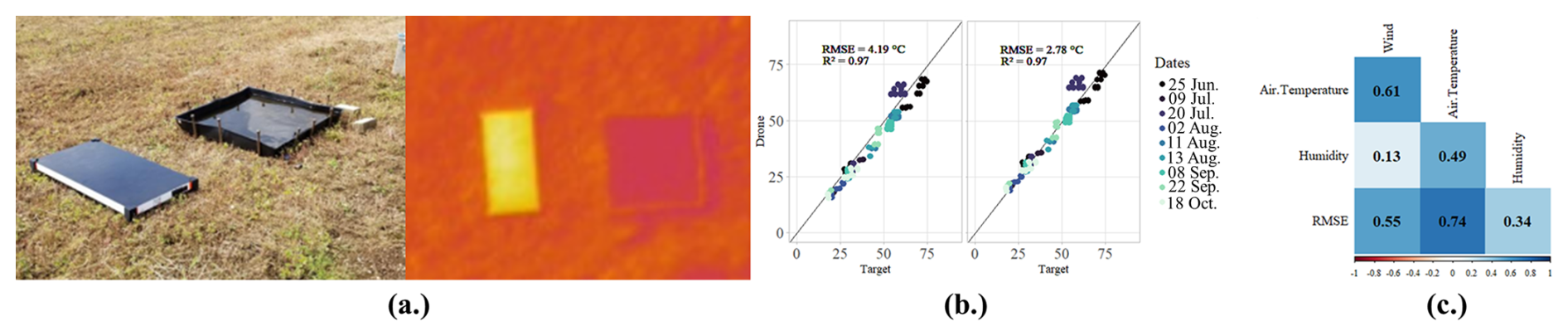
Figure D2(a) ground photo and aerial TIR view of the hot and cold temperature ground reference targets (b) pre-correction and post-correction graphed RMSE of TIR images in the 2021 season (c) correlation of weather factors with RMSE.
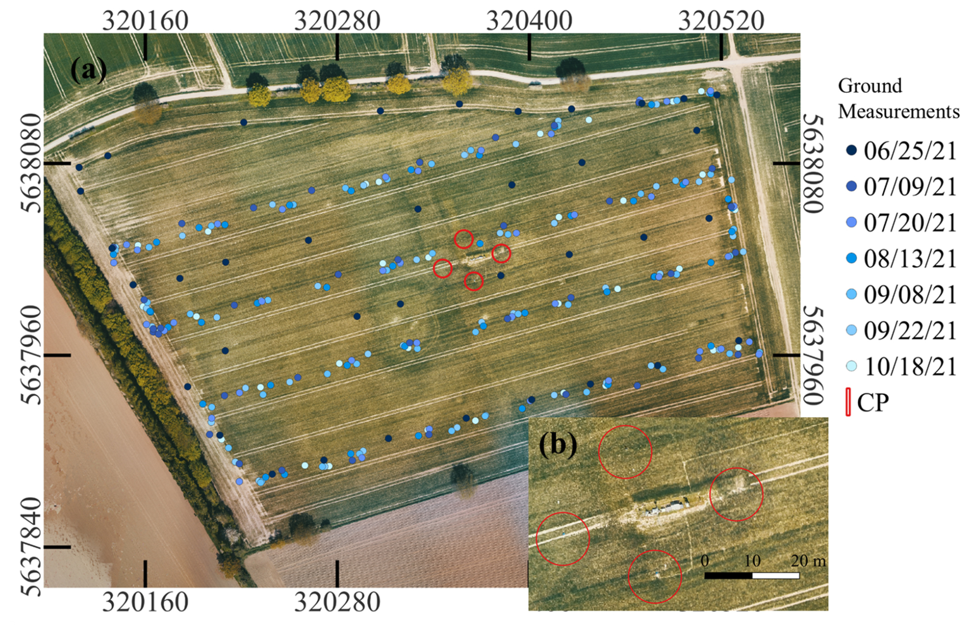
Figure D3(Left) Location of continuous measurement plots (CP) around climate station in the middle of the experiment field site. (Right) Crop height measuring locations for the listed 2021 campaigns by color.
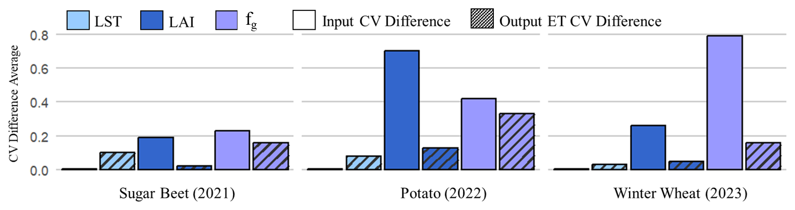
Figure D4Comparison of average differences in the coefficient of variation (CV) between key TSEB-PT input variables (LST, LAI, fg) and the resulting ET estimates across three crop types. This highlights how changes in the spatial variability of each input affect the spatial variability of modeled ET. The CV difference for fg reflects the transition from a uniform value (fg=1) to a spatially variable product derived from the fusion of GAI and PAI.
Table D1The following TIR and MS collection dates with the relevant weather conditions during each flight that may have contributing factors on the accuracy of the observations.
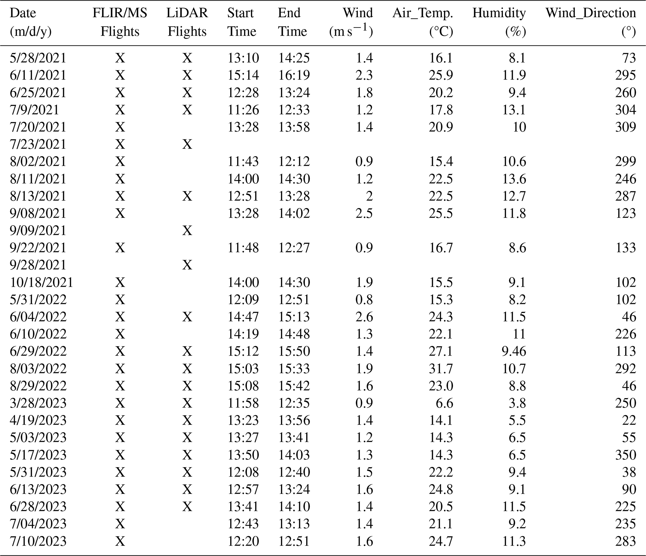
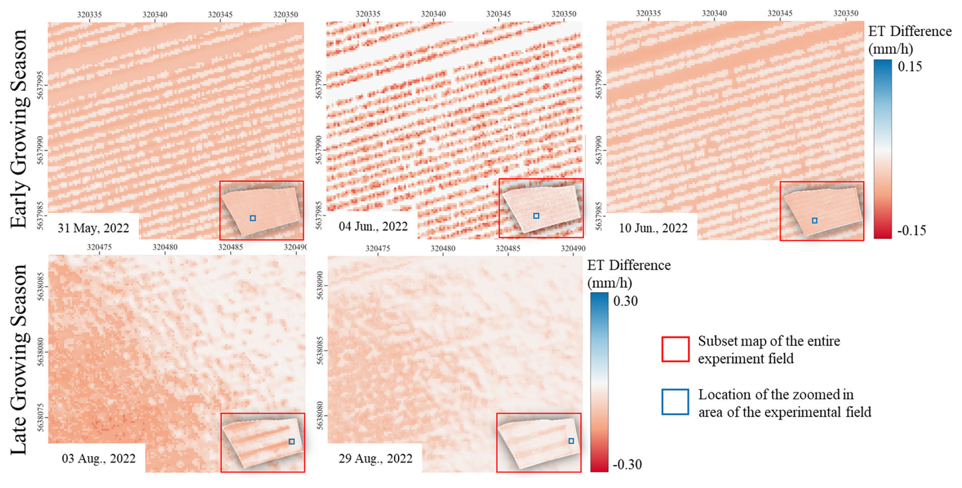
Figure D5Difference in TSEB-PT ET estimates using original land surface temperature (LSTOG) ET minus reference target corrected (LSTTC; ETOG − ETTC) ET. The maps illustrate how the magnitude and spatial pattern of ET differences vary with dominant evaporative sources (soil vs. canopy) and crop water stress conditions. The zoomed-in area is outlined in blue within the full experimental field (red). Late-season areas are located along the edge of a potential water-limited zone, highlighting differences in ET response between stressed and non-stressed regions under varying LST inputs.
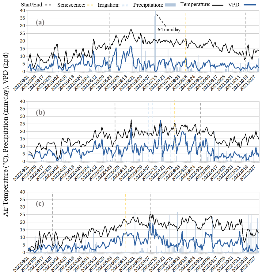
Figure D6Daily air temperature, precipitation, and vapor pressure deficit (VPD) for the following years (a) 2021, (b) 2022, and (c) 2023.
Table D2Summary of flux comparison statistics for net radiation (Rn), latent heat flux (LE), sensible heat flux (H), and soil heat flux (G) derived from TSEB model runs using UAV-based inputs. Model configurations include original and temperature-corrected LST, with additional inputs of LAI = GAI and fg=1. Results are presented for three growing seasons: 2021 (sugar beet), 2022 (potato), and 2023 (winter wheat), covering the full growing period. For each season, statistics are shown for both the complete dataset and for periods excluding senescence. Comparisons are provided against eddy covariance (EC) measurements under both open energy balance conditions and Bowen ratio–closed energy balance conditions.
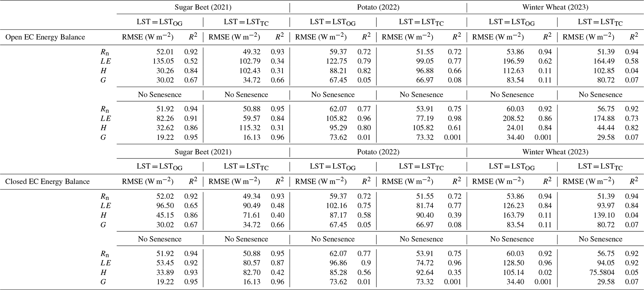
Table D3Summary of flux comparison statistics for net radiation (Rn), latent heat flux (LE), sensible heat flux (H), and soil heat flux (G) derived from TSEB model runs using UAV-based inputs. Model configurations include (i) variation in LAI input (GAI vs. PAI) with LST = LSTTC and fg=1, and (ii) implementation of a dynamic fg (GAI PAI) with LST = LSTTC and LAI = PAI. Results are presented for three growing seasons: 2021 (sugar beet), 2022 (potato), and 2023 (winter wheat), covering the full growing period. For each season, statistics are shown for both the complete dataset and for periods excluding senescence. Comparisons are provided against eddy covariance (EC) measurements under both open energy balance conditions and Bowen ratio–closed energy balance conditions.
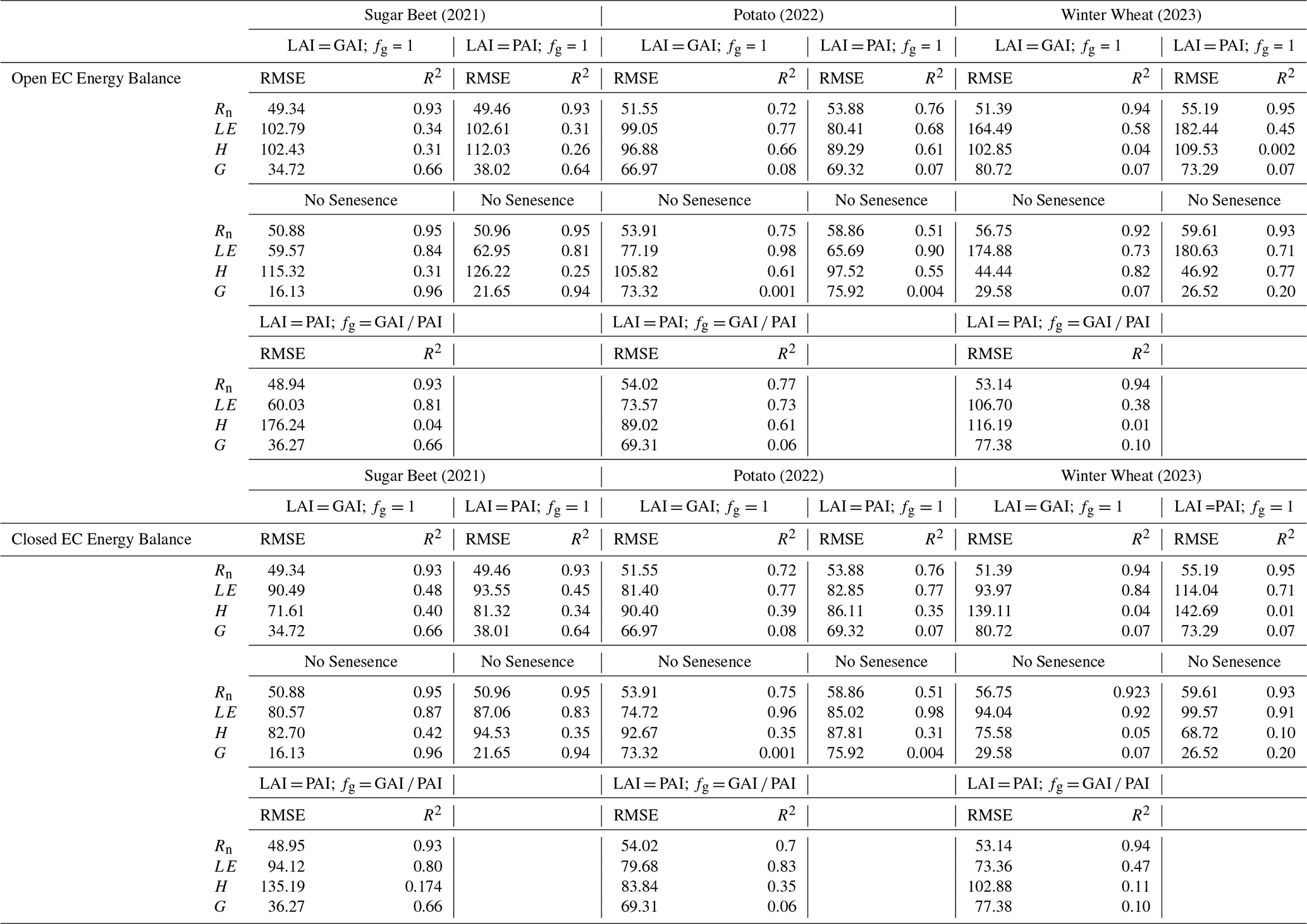
TSEB-PT simulations were performed using the open-source pyTSEB package (https://doi.org/10.5281/zenodo.594732, Nieto et al., 2018), available at http://www.github.com/hectornieto/pytseb, last access: 1 March 2024. Eddy covariance flux footprints were calculated using the Flux Footprint Prediction (FFP) model of Kljun et al. (2015), available at https://www.footprint.kljun.net, last access: 1 November 2023.
The processed UAV-derived spatial datasets used as inputs to TSEB-PT in this study are publicly available through Zenodo at https://doi.org/10.5281/zenodo.23056700 (Bates et al., 2026a). Eddy covariance, meteorological, and ground-reference data used in this study are available through the ICOS Carbon Portal and are cited in the reference list (https://hdl.handle.net/11676/-6oQN2W3wkdiVa0M-dWohuCG, Schmidt et al., 2025a; https://hdl.handle.net/11676/rmxzviWfbl64eSzQyqaQM8nB, Schmidt et al., 2025b).
JSB, FJ, and CM conceived and designed the study. JSB collected the UAV and field data, performed the data processing and analysis, and wrote the original manuscript. CM, HV, and FJ contributed to manuscript review and editing. FJ, CM, and HV supervised the research and acquired funding. All authors read and approved the final version of the manuscript.
The contact author has declared that none of the authors has any competing interests.
Publisher's note: Copernicus Publications remains neutral with regard to jurisdictional claims made in the text, published maps, institutional affiliations, or any other geographical representation in this paper. The authors bear the ultimate responsibility for providing appropriate place names. Views expressed in the text are those of the authors and do not necessarily reflect the views of the publisher.
Additional support was provided by the Helmholtz Association through the Modular Observation Solutions for Earth Systems (MOSES) Initiative and by the Space4ReLaunch project, which is supported by the SPW Economie Emploi Recherche of the Walloon Region under grant agreement no. 2210181. The authors gratefully acknowledge Marius Schmidt and his team for providing the ground-based LAI and crop height validation measurements. The authors also thank Héctor Nieto for the development and maintenance of pyTSEB and for his time and helpful guidance regarding model implementation and interpretation.
This research was primarily supported by the Deutsche Forschungsgemeinschaft (DFG, German Research Foundation) under Germany's Excellence Strategy (grant no. EXC 2070-390732324).
The article processing charges for this open-access publication were covered by the Forschungszentrum Jülich.
This paper was edited by Mallory Barnes and reviewed by William Kustas and one anonymous referee.
Aboutalebi, M., Torres-Rua, A. F., McKee, M., Nieto, H., Kustas, W., and Coopmans, C.: The impact of shadows on partitioning of radiometric temperature to canopy and soil temperature based on the contextual two-source energy balance model (TSEB-2T), P. Soc. Photo.-Opt. Ins., 11008, https://doi.org/10.1117/12.2519685, 2019.
Acharya, B. and Sharma, V.: Comparison of Satellite Driven Surface Energy Balance Models in Estimating Crop Evapotranspiration in Semi-Arid to Arid Inter-Mountain Region, Remote Sensing, 13, https://doi.org/10.3390/rs13091822, 2021.
Ali, M., Montzka, C., Stadler, A., Menz, G., Thonfeld, F., and Vereecken, H.: Estimation and Validation of RapidEye-Based Time-Series of Leaf Area Index for Winter Wheat in the Rur Catchment (Germany), Remote Sensing, 7, 2808–2831, https://doi.org/10.3390/rs70302808, 2015.
Allen, R. G., Pereira, L. S., Raes, D., and Smith, M.: Crop evapotranspiration – Guidelines for computing crop water requirements, FAO Irrigation and Drainage Paper 56, Food and Agriculture Organization of the United Nations, Rome, https://www.fao.org/4/X0490E/X0490E00.htm (last access: 15 March 2026), 1998.
Amani, S. and Shafizadeh-Moghadam, H.: A review of machine learning models and influential factors for estimating evapotranspiration using remote sensing and ground-based data, Agr. Water Manage., 284, 108324, https://doi.org/10.1016/j.agwat.2023.108324, 2023.
Amin, E., Verrelst, J., Rivera-Caicedo, J. P., Pipia, L., Ruiz-Verdú, A., and Moreno, J.: Prototyping Sentinel-2 green LAI and brown LAI products for cropland monitoring, Remote Sens. Environ., 255, 112168, https://doi.org/10.1016/j.rse.2020.112168, 2021.
Anderson, M. C., Kustas, W. P., Norman, J. M., Diak, G. T., Hain, C. R., Gao, F., Yang, Y., Knipper, K. R., Xue, J., Yang, Y., Crow, W. T., Holmes, T. R. H., Nieto, H., Guzinski, R., Otkin, J. A., Mecikalski, J. R., Cammalleri, C., Torres-Rua, A. T., Zhan, X., Fang, L., Colaizzi, P. D., and Agam, N.: A brief history of the thermal IR-based Two-Source Energy Balance (TSEB) model – diagnosing evapotranspiration from plant to global scales, Agr. Forest Meteorol., 350, 109951, https://doi.org/10.1016/j.agrformet.2024.109951, 2024.
Ankela, C. B., Neelima, T. L., Chandrasekar, K., Misra, C., Avil Kumar, K., and Noorzai, A.: Spatiotemporal assessment of maize evapotranspiration and surface energy fluxes under varying irrigation regimes using UAV based METRIC, Sci. Rep., 16, 4302, https://doi.org/10.1038/s41598-025-33916-5, 2026.
Bates, J., Montzka, C., Vereecken, H., and Jonard, F.: UAV Multi-Sensor Derived Inputs for TSEB-PT Evapotranspiration Estimation in Sugar Beet, Potato, and Winter Wheat, Zenodo [data set], https://doi.org/10.5281/zenodo.23056700, 2026a.
Bates, J. S., Montzka, C., Schmidt, M., and Jonard, F.: Estimating Canopy Density Parameters Time-Series for Winter Wheat Using UAS Mounted LiDAR, Remote Sensing, 13, 352, https://doi.org/10.3390/rs13030352, 2021.
Bates, J. S., Montzka, C., Bajracharya, R., Vereecken, H., and Jonard, F.: Wheat biomass estimation across crop development using UAV LiDAR structure–intensity fusion alongside multispectral and thermal data, Biogeosciences, 23, 6179–6210, https://doi.org/10.5194/bg-23-6179-2026, 2026b.
Bellvert, J., Jofre-Ĉekalović, C., Pelechá, A., Mata, M., and Nieto, H.: Feasibility of Using the Two-Source Energy Balance Model (TSEB) with Sentinel-2 and Sentinel-3 Images to Analyze the Spatio-Temporal Variability of Vine Water Status in a Vineyard, Remote Sensing, 12, 2299, https://doi.org/10.3390/rs12142299, 2020.
Bozorgi, M., Cristóbal, J., and Pàmies-Sans, M.: Evaluating the Two-Source Energy Balance Model Using MODIS Data for Estimating Evapotranspiration Time Series on a Regional Scale, Remote Sensing, 16, 4587, https://doi.org/10.3390/rs16234587, 2024.
Brenner, C., Thiem, C. E., Wizemann, H.-D., Bernhardt, M., and Schulz, K.: Estimating spatially distributed turbulent heat fluxes from high-resolution thermal imagery acquired with a UAV system, Int. J. Remote Sens., 38, 3003–3026, https://doi.org/10.1080/01431161.2017.1280202, 2017.
Brenner, C., Zeeman, M., Bernhardt, M., and Schulz, K.: Estimation of evapotranspiration of temperate grassland based on high-resolution thermal and visible range imagery from unmanned aerial systems, Int. J. Remote Sens., 39, 5141–5174, 2018.
Brogi, C., Huisman, J. A., Herbst, M., Weihermüller, L., Klosterhalfen, A., Montzka, C., Reichenau, T. G., and Vereecken, H.: Simulation of spatial variability in crop leaf area index and yield using agroecosystem modeling and geophysics-based quantitative soil information, Vadose Zone J., 19, e20009, https://doi.org/10.1002/vzj2.20009, 2020.
Budzier, H. and Gerlach, G.: Calibration of uncooled thermal infrared cameras, J. Sens. Sens. Syst., 4, 187–197, https://doi.org/10.5194/jsss-4-187-2015, 2015.
Bukowiecki, J., Rose, T., Ehlers, R., and Kage, H.: High-Throughput Prediction of Whole Season Green Area Index in Winter Wheat With an Airborne Multispectral Sensor, Front. Plant Sci., 10, 1798, https://doi.org/10.3389/fpls.2019.01798, 2020.
Burchard-Levine, V., Nieto, H., Riaño, D., Migliavacca, M., El-Madany, T. S., Guzinski, R., Carrara, A., and Martín, M. P.: The effect of pixel heterogeneity for remote sensing-based retrievals of evapotranspiration in a semi-arid tree–grass ecosystem, Remote Sens. Environ., 260, 112440, https://doi.org/10.1016/j.rse.2021.112440, 2021.
Cammalleri, C., Anderson, M. C., and Kustas, W. P.: Upscaling of evapotranspiration fluxes from instantaneous to daytime scales for thermal remote sensing applications, Hydrol. Earth Syst. Sci., 18, 1885–1894, https://doi.org/10.5194/hess-18-1885-2014, 2014.
Campbell, G. S.: Derivation of an angle density function for canopies with ellipsoidal leaf angle distributions, Agr. Forest Meteorol., 49, 173–176, 1990.
Campbell, G. S. and Norman, J. M.: An Introduction to Environmental Biophysics, 2nd edn., Springer, New York, https://doi.org/10.1007/978-1-4612-1626-1, 1998.
Cao, L., Liu, H., Fu, X., Zhang, Z., Shen, X., and Ruan, H.: Comparison of UAV LiDAR and Digital Aerial Photogrammetry Point Clouds for Estimating Forest Structural Attributes in Subtropical Planted Forests, Forests, 10, 145, https://doi.org/10.3390/f10020145, 2019.
Chandel, A. K., Molaei, B., Khot, L. R., Peters, R. T., and Stöckle, C. O.: High Resolution Geospatial Evapotranspiration Mapping of Irrigated Field Crops Using Multispectral and Thermal Infrared Imagery with METRIC Energy Balance Model, Drones, 4, 52, https://doi.org/10.3390/drones4030052, 2020.
Chirouze, J., Boulet, G., Jarlan, L., Fieuzal, R., Rodriguez, J. C., Ezzahar, J., Er-Raki, S., Bigeard, G., Merlin, O., Garatuza-Payan, J., Watts, C., and Chehbouni, G.: Intercomparison of four remote-sensing-based energy balance methods to retrieve surface evapotranspiration and water stress of irrigated fields in semi-arid climate, Hydrol. Earth Syst. Sci., 18, 1165–1188, https://doi.org/10.5194/hess-18-1165-2014, 2014.
Choudhury, B. J., Idso, S. B., and Reginato, R. J.: Analysis of an empirical model for soil heat flux under a growing wheat crop for estimating evaporation by an infrared-temperature based energy balance equation, Agr. Forest Meteorol., 39, 283–297, 1987.
Colaizzi, P.: Advances in a Two-Source Energy Balance Model: Partitioning of Evaporation and Transpiration for Cotton, T. ASABE, 59, 181–197, 2016.
Colaizzi, P. D., Agam, N., Tolk, J. A., Evett, S. R., and Howell, T. A.: Two-Source Energy Balance Model to Calculate E, T, and ET: Comparison of Priestley-Taylor and Penman-Monteith Formulations and Two Time Scaling Methods, T. ASABE, 479–498, https://doi.org/10.13031/trans.57.10423, 2014.
de Lima, G. S. A., Ferreira, M. E., Sales, J. C., de Souza Passos, J., Maggiotto, S. R., Madari, B. E., de Melo Carvalho, M. T., and de Almeida Machado, P. L. O.: Evapotranspiration measurements in pasture, crops, and native Brazilian Cerrado based on UAV-borne multispectral sensor, Environ. Monit. Assess., 196, 1105, https://doi.org/10.1007/s10661-024-13224-7, 2024.
Derardja, B., Khadra, R., Abdelmoneim, A. A. A., El-Shirbeny, M. A., Valsamidis, T., De Pasquale, V., Deflorio, A. M., and Volden, E.: Advancements in Remote Sensing for Evapotranspiration Estimation: A Comprehensive Review of Temperature-Based Models, Remote Sensing, 16, 11, https://doi.org/10.3390/rs16111927, 2024.
Dreier, A., Lopez, G., Bajracharya, R., Kuhlmann, H., and Klingbeil, L.: Structural wheat trait estimation using UAV-based laser scanning data: Analysis of critical aspects and recommendations based on a case study, Precis. Agric., 26, 18, https://doi.org/10.1007/s11119-024-10202-4, 2025.
Duran-Gomez, M. R., Torres-Rua, A., Hipps, L., Kustas, W., Bambach, N. E., Knipper, K., Wright, I., McElrone, A. J., Prueger, J. H., Alfieri, J. G., Coopmans, C., Meza, K., Gowing, I., Nocco, M., Castro, S. J., Gal, A., and Tolentino, P.: Influence of almond's canopy-induced shadows on actual evapotranspiration estimation by the TSEB model using sUAS multispectral and thermal imagery, Irrigation Sci., 44, 54, https://doi.org/10.1007/s00271-026-01092-7, 2026.
Ebert, L. A., Talib, A., Zipper, S. C., Desai, A. R., U, K. T. P., Chisholm, A. J., Prater, J., and Nocco, M. A.: How High to Fly? Mapping Evapotranspiration from Remotely Piloted Aircrafts at Different Elevations, Remote Sensing, 14, https://doi.org/10.3390/rs14071660, 2022.
El Hazdour, I., Le Page, M., Hanich, L., Chakir, A., Lopez, O., and Jarlan, L.: A GEE TSEB workflow for daily high-resolution fully remote sensing evapotranspiration: Validation over four crops in semi-arid conditions and comparison with the SSEBop experimental product, Environ. Modell. Softw., 187, 106365, https://doi.org/10.1016/j.envsoft.2025.106365, 2025.
Elfarkh, J., Ezzahar, J., Er-Raki, S., Simonneaux, V., Ait Hssaine, B., Rachidi, S., Brut, A., Rivalland, V., Khabba, S., Chehbouni, A., and Jarlan, L.: Multi-Scale Evaluation of the TSEB Model over a Complex Agricultural Landscape in Morocco, Remote Sensing, 12, 1181, https://doi.org/10.3390/rs12071181, 2020.
Elfarkh, J., Johansen, K., El Hajj, M. M., Almashharawi, S. K., and McCabe, M. F.: Evapotranspiration, gross primary productivity and water use efficiency over a high-density olive orchard using ground and satellite based data, Agr. Water Manage., 287, 108423, https://doi.org/10.1016/j.agwat.2023.108423, 2023.
Ellsäßer, F., Röll, A., Stiegler, C., Hendrayanto, and Hölscher, D.: Introducing QWaterModel, a QGIS plugin for predicting evapotranspiration from land surface temperatures, Environ. Modell. Softw., 130, 104739, https://doi.org/10.1016/j.envsoft.2020.104739, 2020.
Flint, E. A., Hopkins, B. G., Svedin, J. D., Kerry, R., Heaton, M. J., Jensen, R. R., Campbell, C. S., Yost, M. A., and Hansen, N. C.: Irrigation Zone Delineation and Management with a Field-Scale Variable Rate Irrigation System in Winter Wheat, Agronomy, 13, https://doi.org/10.3390/agronomy13041125, 2023.
Gao, R., Torres-Rua, A., Nassar, A., Alfieri, J., Aboutalebi, M., Hipps, L., Ortiz, N. B., McElrone, A. J., Coopmans, C., Kustas, W., White, W., McKee, L., Alsina, M. del M., Dokoozlian, N., Sanchez, L., Prueger, J. H., Nieto, H., and Agam, N.: Evapotranspiration partitioning assessment using a machine-learning-based leaf area index and the two-source energy balance model with sUAV information, Autonomous Air and Ground Sensing Systems for Agricultural Optimization and Phenotyping VI, 11747, 117470N, https://doi.org/10.1117/12.2586259, 2021.
Gao, R., Torres-Rua, A. F., Nieto, H., Zahn, E., Hipps, L., Kustas, W. P., Alsina, M. M., Bambach, N., Castro, S. J., Prueger, J. H., Alfieri, J., McKee, L. G., White, W. A., Gao, F., McElrone, A. J., Anderson, M., Knipper, K., Coopmans, C., Gowing, I., Agam, N., Sanchez, L., and Dokoozlian, N.: ET Partitioning Assessment Using the TSEB Model and sUAS Information across California Central Valley Vineyards, Remote Sens., 15, 756, https://doi.org/10.3390/rs15030756, 2023.
García-Santos, V., Sánchez, J. M., and Cuxart, J.: Evapotranspiration Acquired with Remote Sensing Thermal-Based Algorithms: A State-of-the-Art Review, Remote Sensing, 14, 3440, https://doi.org/10.3390/rs14143440, 2022.
Ghiat, I., Mackey, H. R., and Al-Ansari, T.: A Review of Evapotranspiration Measurement Models, Techniques and Methods for Open and Closed Agricultural Field Applications, Water, 13, 2523, https://doi.org/10.3390/w13182523, 2021.
Giardina, F., Gentine, P., Konings, A. G., Seneviratne, S. I., and Stocker, B. D.: Diagnosing evapotranspiration responses to water deficit across biomes using deep learning, New Phytol., 240, 968–983, https://doi.org/10.1111/nph.19197, 2023.
Gogler, S., Madura, H., Krupiński, M., Bieszczad, G., and Sosnowski, T.: Non-Uniformity Correction in Microbolometer Array with Temperature Influence Compensation, Metrol. Meas. Syst., 2014, 709–718, 2014.
Guzinski, R., Nieto, H., Sandholt, I., and Karamitilios, G.: Modelling High-Resolution Actual Evapotranspiration through Sentinel-2 and Sentinel-3 Data Fusion, Remote Sensing, 12, 9, https://doi.org/10.3390/rs12091433, 2020.
Gómez-Candón, D., Bellvert, J., and Royo, C.: Performance of the Two-Source Energy Balance (TSEB) Model as a Tool for Monitoring the Response of Durum Wheat to Drought by High-Throughput Field Phenotyping, Front. Plant Sci., 12, https://doi.org/10.3389/fpls.2021.658357, 2021.
Han, X., Thomasson, J. A., Swaminathan, V., Wang, T., Siegfried, J., Raman, R., Rajan, N., and Neely, H.: Field-Based Calibration of Unmanned Aerial Vehicle Thermal Infrared Imagery with Temperature-Controlled References, Sensors, 20, 7098, https://doi.org/10.3390/s20247098, 2020.
Heinemann, S., Siegmann, B., Thonfeld, F., Muro, J., Jedmowski, C., Kemna, A., Kraska, T., Muller, O., Schultz, J., Udelhoven, T., Wilke, N., and Rascher, U.: Land Surface Temperature Retrieval for Agricultural Areas Using a Novel UAV Platform Equipped with a Thermal Infrared and Multispectral Sensor, Remote Sensing, 12, https://doi.org/10.3390/rs12071075, 2020.
Hirschi, M., Michel, D., Lehner, I., and Seneviratne, S. I.: A site-level comparison of lysimeter and eddy covariance flux measurements of evapotranspiration, Hydrol. Earth Syst. Sci., 21, 1809–1825, https://doi.org/10.5194/hess-21-1809-2017, 2017.
Hoffmann, H., Nieto, H., Jensen, R., Guzinski, R., Zarco-Tejada, P., and Friborg, T.: Estimating evaporation with thermal UAV data and two-source energy balance models, Hydrol. Earth Syst. Sci., 20, 697–713, https://doi.org/10.5194/hess-20-697-2016, 2016.
Hunt Jr., E. R. and Daughtry, C. S. T.: What good are unmanned aircraft systems for agricultural remote sensing and precision agriculture?, Int. J. Remote Sens., 39, 5345–5376, 2018.
Hütt, C., Bolten, A., Hüging, H., and Bareth, G.: UAV LiDAR Metrics for Monitoring Crop Height, Biomass and Nitrogen Uptake: A Case Study on a Winter Wheat Field Trial, PFG – Journal of Photogrammetry, Remote Sensing and Geoinformation Science, 91, 65–76, https://doi.org/10.1007/s41064-022-00228-6, 2022.
Jaafar, H. H. and Sujud, H. L.: High resolution evapotranspiration from UAV multispectral thermal imagery: Validation and comparison with EC, Landsat, and fused S2-MODIS HSEB ET, Int. J. Appl. Earth Obs., 136, 104359, https://doi.org/10.1016/j.jag.2025.104359, 2025.
Jaafar, H. H., Mourad, R. M., Kustas, W. P., and Anderson, M. C.: A Global Implementation of Single- and Dual-Source Surface Energy Balance Models for Estimating Actual Evapotranspiration at 30-m Resolution Using Google Earth Engine, Water Resour. Res., 58, e2022WR032800, https://doi.org/10.1029/2022WR032800, 2022.
Jia, K., Li, Y., Liang, S., Wei, X., and Yao, Y.: Combining Estimation of Green Vegetation Fraction in an Arid Region from Landsat 7 ETM+ Data, Remote Sensing, 9, 1121, https://doi.org/10.3390/rs9111121, 2017.
Jonard F., De Cannière S., Brüggemann N., Gentine P., Short Gianotti D. J., Lobet G., Miralles D. J., Montzka C., Pagán B. R., Rascher U., and Vereecken, H.: Value of chlorophyll fluorescence for quantifying hydrological states and fluxes: Current status and challenges, Agr. Forest Meteorol., 291, 108088, https://doi.org/10.1016/j.agrformet.2020.108088, 2020.
Kavya, B. M. and Mahadevaiah, T.: Enhancing Estimation Of Evapotranspiration In Sugarcane Cultivation Using Lysimeter Data And Deep Learning Techniques, International Journal of Intelligent Systems and Applications in Engineering, 12, https://www.ijisae.org/index.php/IJISAE/article/view/7232 (last access: 13 October 2026), 2024.
Kelly, J., Kljun, N., Olsson, P.-O., Mihai, L., Liljeblad, B., Weslien, P., Klemedtsson, L., and Eklundh, L.: Challenges and Best Practices for Deriving Temperature Data from an Uncalibrated UAV Thermal Infrared Camera, Remote Sensing, 11, 567, https://doi.org/10.3390/rs11050567, 2019.
Kljun, N., Calanca, P., Rotach, M. W., and Schmid, H. P.: A simple two-dimensional parameterisation for Flux Footprint Prediction (FFP), Geosci. Model Dev., 8, 3695–3713, https://doi.org/10.5194/gmd-8-3695-2015, 2015.
Kool, D., Kustas, W. P., Ben-Gal, A., and Agam, N.: Energy partitioning between plant canopy and soil, performance of the two-source energy balance model in a vineyard, Agr. Forest Meteorol., 300, 108328, https://doi.org/10.1016/j.agrformet.2021.108328, 2021.
Kustas, W. and Anderson, M.: Advances in thermal infrared remote sensing for land surface modeling, Agr. Forest Meteorol., 149, 2071–2081, 2009.
Kustas, W. P. and Daughtry, C. S. T.: Estimation of the soil heat flux/net radiation ratio from spectral data, Agr. Forest Meteorol., 49, 205–223, 1990.
Kustas, W. P. and Norman, J. M.: Evaluation of soil and vegetation heat flux predictions using a simple two-source model with radiometric temperatures for partial canopy cover, Agr. Forest Meteorol., 94, 13–29, 1999.
Kustas, W. P., Nieto, H., Morillas, L., Anderson, M. C., Alfieri, J. G., Hipps, L. E., Villagarcía, L., Domingo, F., and Garcia, M.: Revisiting the paper “Using radiometric surface temperature for surface energy flux estimation in Mediterranean drylands from a two-source perspective.”, Remote Sens. Environ., 184, 645–653, 2016.
Li, Y., Kustas, W. P., Huang, C., Nieto, H., Haghighi, E., Anderson, M. C., Domingo, F., Garcia, M., and Scott, R. L.: Evaluating Soil Resistance Formulations in Thermal-Based Two-Source Energy Balance (TSEB) Model: Implications for Heterogeneous Semiarid and Arid Regions, Water Resour. Res., 55, 1059–1078, 2019.
Liu, Y., Zhang, S., Zhang, J., Tang, L., and Bai, Y.: Assessment and Comparison of Six Machine Learning Models in Estimating Evapotranspiration over Croplands Using Remote Sensing and Meteorological Factors, Remote Sensing, 13, 19, https://doi.org/10.3390/rs13193838, 2021.
Liu, H., Song, W., Lv, J., Gui, R., Shi, Y., Lu, Y., Li, M., Chen, L., and Chen, X.: Precise Drought Threshold Monitoring in Winter Wheat Using the Unmanned Aerial Vehicle Thermal Method, Remote Sensing, 16, 4, https://doi.org/10.3390/rs16040710, 2024.
Liyew, C. M., Ferraris, S., Di Nardo, E., and Meo, R.: A review of feature selection methods for actual evapotranspiration prediction, Artif. Intell. Rev., 58, 292, https://doi.org/10.1007/s10462-025-11298-4, 2025.
Lu, S., Xuan, J., Zhang, T., Bai, X., Tian, F., and Ortega-Farias, S.: Effect of the Shadow Pixels on Evapotranspiration Inversion of Vineyard: A High-Resolution UAV-Based and Ground-Based Remote Sensing Measurements, Remote Sensing, 14, https://doi.org/10.3390/rs14092259, 2022.
Lun, S., Liu, T., Bao, Y., Hao, L., Duan, L., Zhang, W., Zhang, S., Zhang, Y., Singh, V. P., and Wang, D.: Resistance optimization and applicability of the TSEB model in desert–oasis areas, Agr. Water Manage., 326, 110231, https://doi.org/10.1016/j.agwat.2026.110231, 2026.
Ma, H., Song, J., and Wang, J.: Forest canopy LAI and vertical FAVD profile inversion from airborne full-waveform LiDAR data based on a radiative transfer model, Remote Sensing, 7, 1897–1914, https://doi.org/10.3390/rs70201897, 2015.
Mendiguren, G., Koch, J., and Stisen, S.: Spatial pattern evaluation of a calibrated national hydrological model – a remote-sensing-based diagnostic approach, Hydrol. Earth Syst. Sci., 21, 5987–6005, https://doi.org/10.5194/hess-21-5987-2017, 2017.
Mohan, M. M. P., Kanchirapuzha, R., and Varma, M. R. R.: Review of approaches for the estimation of sensible heat flux in remote sensing-based evapotranspiration models, J. Appl. Remote Sens., 14, 041501, https://doi.org/10.1117/1.JRS.14.041501, 2020.
Mokhtari, A., Ahmadi, A., Daccache, A., and Drechsler, K.: Actual Evapotranspiration from UAV Images: A Multi-Sensor Data Fusion Approach, Remote Sensing, 13, 2315, https://doi.org/10.3390/rs13122315, 2021.
Montzka, C., Donat, M., Raj, R., Welter, P., and Bates, J. S.: Sensitivity of LiDAR Parameters to Aboveground Biomass in Winter Spelt, Drones, 7, 121, https://doi.org/10.3390/drones7020121, 2023.
Nassar, A., Torres-Rua, A., Kustas, W., Nieto, H., McKee, M., Hipps, L., Stevens, D., Alfieri, J., Alsina, M., McKee, L., Coopmans, C., Sanchez, L., and Dokoozlian, N.: Influence of Model Grid Size on the Estimation of Surface Fluxes Using the Two Source Energy Balance Model and sUAS Imagery in Vineyards, Remote Sensing, 12, 342, https://doi.org/10.3390/rs12030342, 2020.
Nassar, A., Torres-Rua, A., Kustas, W., Alfieri, J., Hipps, L., Prueger, J., Nieto, H., Alsina, M. M., White, W., McKee, L., Coopmans, C., Sanchez, L., and Dokoozlian, N.: Assessing Daily Evapotranspiration Methodologies from One-Time-of-Day sUAS and EC Information in the GRAPEX Project, Remote Sensing, 13, 2887, https://doi.org/10.3390/rs13152887, 2021.
Nassar, A., Torres-Rua, A., Hipps, L., Kustas, W., McKee, M., Stevens, D., Nieto, H., Keller, D., Gowing, I., and Coopmans, C.: Using Remote Sensing to Estimate Scales of Spatial Heterogeneity to Analyze Evapotranspiration Modeling in a Natural Ecosystem, Remote Sensing, 14, 372, https://doi.org/10.3390/rs14020372, 2022.
Nieto, H., Guzinski, R., and Kustas, W. P.: pyTSEB: A Python Two Source Energy Balance model for estimation of evapotranspiration with remote sensing data, version 2.2, Zenodo [code], https://doi.org/10.5281/zenodo.594732, 2018.
Nieto, H., Kustas, W. P., Torres-Rúa, A., Alfieri, J. G., Gao, F., Anderson, M. C., White, W. A., Song, L., Alsina, M. M., Prueger, J. H., McKee, M., Elarab, M., and McKee, L. G.: Evaluation of TSEB turbulent fluxes using different methods for the retrieval of soil and canopy component temperatures from UAV thermal and multispectral imagery, Irrigation Sci., 37, 389–406, 2019.
Nieto, H., Alsina, M. M., Kustas, W. P., García-Tejera, O., Chen, F., Bambach, N., Gao, F., Alfieri, J. G., Hipps, L. E., Prueger, J. H., McKee, L. G., Zahn, E., Bou-Zeid, E., McElrone, A. J., Castro, S. J., and Dokoozlian, N.: Evaluating different metrics from the thermal-based two-source energy balance model for monitoring grapevine water stress, Irrigation Sci., 40, 697–713, https://doi.org/10.1007/s00271-022-00790-2, 2022.
Niu, H., Zhao, T., Wang, D., and Chen, Y.: Evapotranspiration Estimation with UAVs in Agriculture: A Review, Preprints.org, https://doi.org/10.20944/preprints201907.0124.v1, 2019.
Niu, H., Hollenbeck, D., Zhao, T., Wang, D., and Chen, Y.: Evapotranspiration Estimation with Small UAVs in Precision Agriculture, Sensors, 20, 6427, https://doi.org/10.3390/s20226427, 2020.
Norman, J. M., Kustas, W. P., and Humes, K. S.: Source approach for estimating soil and vegetation energy fluxes in observations of directional radiometric surface temperature, Agr. Forest Meteorol., 77, 263–293, 1995.
Oguntunde, P., Olukunle, O. J., Fasinmirin, J., and Abiolu, O. A.: Performance of the SunScan canopy analysis system in estimating leaf area index of maize, Agricultural Engineering International: The CIGR Journal, 14, 1–7, https://cigrjournal.org/index.php/Ejounral/article/view/1823 (last access: 13 October 2026),, 2012.
Ortiz, M. S., Ducati, J. R., Espinoza, J., and Monteiro, R. C.: Evapotranspiration Estimate Using Energy Balance Two Source Model With UAV Images: A Study in Vineyard, Am. J. Eng. Res., 8, 60–69, https://www.ajer.org/papers/Vol-8-issue-8/H08086069.pdf (last access: 13 October 2026), 2019.
Park, S., Ryu, D., Fuentes, S., Chung, H., O'Connell, M., and Kim, J.: Mapping Very-High-Resolution Evapotranspiration from Unmanned Aerial Vehicle (UAV) Imagery, ISPRS Int. J. Geo-Inf., 10, https://doi.org/10.3390/ijgi10040211, 2021.
Pereira, A. and Pires, L.: Evapotranspiration and Water Management for Crop Production, https://doi.org/10.5772/20081, 2011.
Sagan, V., Maimaitijiang, M., Sidike, P., Eblimit, K., Peterson, K. T., Hartling, S., Esposito, F., Khanal, K., Newcomb, M., Pauli, D., Ward, R., Fritschi, F., Shakoor, N., and Mockler, T.: UAV-Based High Resolution Thermal Imaging for Vegetation Monitoring, and Plant Phenotyping Using ICI 8640 P, FLIR Vue Pro R 640, and thermoMap Cameras, Remote Sensing, 11, 330, https://doi.org/10.3390/rs11030330, 2019.
Schmidt, M., Bagheri, S., Becker, N., Dolfus, D., Esser, O., Graf, A., Haustein, A., Kettler, M., Kummer, S., and Mattes, J.: ETC L2 Fluxnet (half-hourly) from Selhausen Juelich, 2018-12-31–2025-09-30, ICOS RI [data set], https://hdl.handle.net/11676/-6oQN2W3wkdiVa0M-dWohuCG (last access: 13 October 2026), 2025a.
Schmidt, M., Bagheri, S., Becker, N., Dolfus, D., Esser, O., Graf, A., Haustein, A., Kettler, M., Kummer, S., and Mattes, J.: ETC L2 Meteo from Selhausen Juelich, 2018-12-31–2025-09-30, ICOS RI [data set], https://hdl.handle.net/11676/rmxzviWfbl64eSzQyqaQM8nB (last access: 13 October 2026), 2025b.
Serrano, J., Shahidian, S., Silva, J. M. da, Paixão, L., Moral, F., Carmona-Cabezas, R., Garcia, S., Palha, J., and Noéme, J.: Mapping Management Zones Based on Soil Apparent Electrical Conductivity and Remote Sensing for Implementation of Variable Rate Irrigation – Case Study of Corn under a Center Pivot, Water, 12, https://doi.org/10.3390/w12123427, 2020.
Shi, H. and Cai, X.: Extrapolability improvement of machine learning-based evapotranspiration models via domain-adversarial neural networks, Environ. Modell. Softw., 187, 106383, https://doi.org/10.1016/j.envsoft.2025.106383, 2025.
Song, L., Xu, Y., Liddell, M., Cui, Y., Liu, S., and Xu, P.: Application of a two source energy balance model coupled with satellite based soil moisture and thermal infrared data, ISPRS J. Photogramm., 204, 15–26, https://doi.org/10.1016/j.isprsjprs.2023.08.009, 2023.
Sánchez-Virosta, Á., Sánchez, J. M., Montoya, F., Gómez-Candón, D., González-Piqueras, J., Molina-Medina, A. J., and López-Urrea, R.: Assessment of different remote sensing techniques to estimate the CWSI of almond trees using canopy temperature, Int. J. Appl. Earth Obs., 142, 104737, https://doi.org/10.1016/j.jag.2025.104737, 2025.
Tan, C.-W., Zhang, P.-P., Zhou, X.-X., Wang, Z.-X., Xu, Z.-Q., Mao, W., Li, W.-X., Huo, Z.-Y., Guo, W.-S., and Yun, F.: Quantitative monitoring of leaf area index in wheat of different plant types by integrating NDVI and Beer-Lambert law, Sci. Rep., 10, 929, https://doi.org/10.1038/s41598-020-57750-z, 2020.
Tanner, C. B.: Plant Temperatures, Agron. J., 55, 210–211, 1963.
Tao, S., Song, L., Zhao, G., and Zhao, L.: Simulation and Assessment of Daily Evapotranspiration in the Heihe River Basin over a Long Time Series Based on TSEB-SM, Remote Sensing, 16, 3, https://doi.org/10.3390/rs16030462, 2024.
Thorp, K. R., Hunsaker, D. J., and French, A. N.: Assimilating Leaf Area Index Estimates from Remote Sensing into the Simulations of a Cropping Systems Model, T. ASABE, 53, 251–262, 2010.
Tunca, E.: Evaluating the performance of the TSEB model for sorghum evapotranspiration estimation using time series UAV imagery, Irrigation Sci., 42, 977–994, https://doi.org/10.1007/s00271-023-00887-2, 2023.
Tunca, E.: Evaluating machine learning and deep learning for upscaling instantaneous latent heat flux to daily scale, Irrigation Sci., 44, 40, https://doi.org/10.1007/s00271-026-01079-4, 2026.
Tunca, E., Köksal, E. S., and Taner, S. Ç.: Calibrating UAV thermal sensors using machine learning methods for improved accuracy in agricultural applications, Infrared Phys. Techn., 133, 104804, https://doi.org/10.1016/j.infrared.2023.104804, 2023.
Twine, T. E., Kustas, W. P., Norman, J. M., Cook, D. R., Houser, P. R., Meyers, T. P., Prueger, J. H., Starks, P. J., and Wesely, M. L.: Correcting eddy-covariance flux underestimates over a grassland, Agr. Forest Meteorol., 103, 279–300, https://doi.org/10.1016/S0168-1923(00)00123-4, 2000.
Virtue, J., Turner, D., Williams, G., Zeliadt, S., McCabe, M., and Lucieer, A.: Thermal Sensor Calibration for Unmanned Aerial Systems Using an External Heated Shutter, Drones, 5, 119, https://doi.org/10.3390/drones5040119, 2021.
von Hebel, C., Reynaert, S., Pauly, K., Janssens, P., Piccard, I., Vanderborght, J., van der Kruk, J., Vereecken, H., and Garré, S.: Toward high-resolution agronomic soil information and management zones delineated by ground-based electromagnetic induction and aerial drone data, Vadose Zone J., 20, e20099, https://doi.org/10.1002/vzj2.20099, 2021.
Wan, Q., Smigaj, M., Brede, B., and Kooistra, L.: Optimizing UAV-based uncooled thermal cameras in field conditions for precision agriculture, Int. J. Appl. Earth Obs., 134, 104184, https://doi.org/10.1016/j.jag.2024.104184, 2024.
Wang, W., Zou, S., Luo, Z., Zhang, W., Chen, D., and Kong, J.: Prediction of the Reference Evapotranspiration Using a Chaotic Approach, Sci. World J., 2014, e347625, https://doi.org/10.1155/2014/347625, 2014.
Wanniarachchi, S. and Sarukkalige, R.: A Review on Evapotranspiration Estimation in Agricultural Water Management: Past, Present, and Future, Hydrology, 9, 7, https://doi.org/10.3390/hydrology9070123, 2022.
Wei, J., Dong, W., Liu, S., Song, L., Zhou, J., Xu, Z., Wang, Z., Xu, T., He, X., and Sun, J.: Mapping super high resolution evapotranspiration in oasis-desert areas using UAV multi-sensor data, Agr. Water Manage., 287, 108466, https://doi.org/10.1016/j.agwat.2023.108466, 2023.
Wei, J., Luo, Y., Liu, B., and Cui, Y.: Temporal Upscaling of Agricultural Evapotranspiration with an Improved Evaporative Fraction Method, Remote Sensing, 17, https://doi.org/10.3390/rs17061016, 2025.
Wu, K. and Lambot, S.: Digital Soil Mapping Using Drone-Borne Ground-Penetrating Radar, in: Instrumentation and Measurement Technologies for Water Cycle Management, edited by: Di Mauro, A., Scozzari, A., and Soldovieri, F., Springer International Publishing, 417–436, https://doi.org/10.1007/978-3-031-08262-7_17, 2022.
Xia, T., Kustas, W. P., Anderson, M. C., Alfieri, J. G., Gao, F., McKee, L., Prueger, J. H., Geli, H. M. E., Neale, C. M. U., Sanchez, L., Alsina, M. M., and Wang, Z.: Mapping evapotranspiration with high-resolution aircraft imagery over vineyards using one- and two-source modeling schemes, Hydrol. Earth Syst. Sci., 20, 1523–1545, https://doi.org/10.5194/hess-20-1523-2016, 2016.
Yang, Y.: Remotely Sensed Evapotranspiration, in: Observation and Measurement of Ecohydrological Processes, edited by: Li, X. and Vereecken, H., 2, Springer Berlin Heidelberg, 155–200, ISBN 978-3-662-48297-1, https://doi.org/10.1007/978-3-662-48297-1, 2019.
Yang, Y., Qiu, J., Zhang, R., Huang, S., Chen, S., Wang, H., Luo, J., and Fan, Y.: Intercomparison of Three Two-Source Energy Balance Models for Partitioning Evaporation and Transpiration in Semiarid Climates, Remote Sensing, 10, 1149, https://doi.org/10.3390/rs10071149, 2018.
Yao, Y., Liang, S., Yu, J., Chen, J., Liu, S., Lin, Y., Fisher, J. B., McVicar, T. R., Cheng, J., Jia, K., Zhang, X., Xie, X., Jiang, B., and Sun, L.: A simple temperature domain two-source model for estimating agricultural field surface energy fluxes from Landsat images: Simple ET Method, J. Geophys. Res.-Atmos., 122, 5211–5236, https://doi.org/10.1002/2016JD026370, 2017.
Yue, J., Guo, W., Yang, G., Zhou, C., Feng, H., and Qiao, H.: Method for accurate multi-growth-stage estimation of fractional vegetation cover using unmanned aerial vehicle remote sensing, Plant Methods, 17, https://doi.org/10.1186/s13007-021-00752-3, 2021.
Zhang, L., Zhang, H., Niu, Y., and Han, W.: Mapping Maize Water Stress Based on UAV Multispectral Remote Sensing, Remote Sensing, 11, 605, https://doi.org/10.3390/rs11060605, 2019.
Zheng, G. and Moskal, L. M.: Retrieving Leaf Area Index (LAI) Using Remote Sensing: Theories, Methods and Sensors, Sensors, 9, 2719–2745, https://doi.org/10.3390/s90402719, 2009.
Zheng, C., Wang, S., Chen, J. M., Xiao, J., Chen, J., Zhu, K., and Sun, L.: Modeling transpiration using solar-induced chlorophyll fluorescence and photochemical reflectance index synergistically in a closed-canopy winter wheat ecosystem, Remote Sens. Environ., 302, 113981, https://doi.org/10.1016/j.rse.2023.113981, 2024.
Zoratipour, E., Mohammadi, A. S., and Zoratipour, A.: Evaluation of SEBS and SEBAL algorithms for estimating wheat evapotranspiration (case study: Central areas of Khuzestan province), Applied Water Science, 13, 137, https://doi.org/10.1007/s13201-023-01941-2, 2023.
- Abstract
- Introduction
- Methods
- Results
- Discussion
- Conclusion
- Appendix A: Description of the TSEB-PT model implementation
- Appendix B: Sensor derived metrics
- Appendix C: EC energy balance closure and daily and potential ET
- Appendix D: Additional material
- Code availability
- Data availability
- Author contributions
- Competing interests
- Disclaimer
- Acknowledgements
- Financial support
- Review statement
- References
- Abstract
- Introduction
- Methods
- Results
- Discussion
- Conclusion
- Appendix A: Description of the TSEB-PT model implementation
- Appendix B: Sensor derived metrics
- Appendix C: EC energy balance closure and daily and potential ET
- Appendix D: Additional material
- Code availability
- Data availability
- Author contributions
- Competing interests
- Disclaimer
- Acknowledgements
- Financial support
- Review statement
- References