DMS, MeSH and nanoparticles in semi-controlled deck-borne experiments using Antarctic seawater: on the effect of UV light

Sulfur-containing volatile organic compounds (VOCs) such as dimethyl sulfide (DMS) and methanethiol (MeSH) are of particular interest among oceanic VOCs emitted by the ocean, both for their central role in the marine sulfur cycle and as potential precursors to secondary aerosol formation. However, the quantification of DMS and MeSH emissions as a function of biological components of the ocean under variable environmental factors are still too scarce for reliable future predictions. In this study we report on measurements of DMS, MeSH and nanoparticle concentrations in the headspace of two on-deck Air-Sea Interface Tanks (ASITs). The cover of one ASIT prevented the transmission of UV light below 380 nm in wavelength and we report on the effect of UV light on fluxes and concentrations. These measurements were carried out near the Antarctic Peninsula during the POLAR-CHANGE campaign in summer 2023. Air–sea fluxes inside the ASITs were always positive, i.e. degassing from seawater to air, with DMS and MeSH fluxes averaging 3.03 $\mathrm{pmol}{\mathrm{m}}^{-\mathrm{2}}{\mathrm{s}}^{-\mathrm{1}}$ (F_ASIT-DMS) and 0.64 $\mathrm{pmol}{\mathrm{m}}^{-\mathrm{2}}{\mathrm{s}}^{-\mathrm{1}}$ (F_ASIT-MeSH), respectively. DMS emission did not vary significantly between day and night, but the ratio $F_{\text{ASIT-MeSH}}/(F_{\text{ASIT-DMS}}+F_{\text{ASIT-MeSH}}$) showed a clear maximum at night and a decrease over daytime. Calculated aqueous DMS concentrations showed maxima in the open Southern Ocean north of the Antarctic Peninsula (2.5–3 nM), minima in the Marginal Ice Zone (MIZ) in the Weddell Sea (1 nM) and moderate values along the western coast of the peninsula (around 1.5–2 nM). Bacterial concentrations showed positive correlations with calculated aqueous DMS and MeSH concentrations during two experiments when seawater was held in the ASITs for 2 d. Removal of UV light increased DMS fluxes by 24 % and MeSH fluxes by 58 %. New particle formation occurred only in the absence of UV-light. Interestingly, the highest impact of UV removal, especially on increased MeSH emission, was seen during the night suggesting a lag period between the exposure and the physiological response of the cells. UV light caused slight nanophytoplankton light stress at noon, which negatively affected the short-term growth of nanophytoplankton, especially in open Southern Ocean waters.

1 Introduction

Various volatile organic compounds (VOCs) are emitted from the surface of the ocean and are now considered key in understanding marine-atmosphere interactions and atmospheric chemistry. Among the wide variety of VOCs emitted by the oceans, sulfur-containing compounds such as dimethyl sulfide (DMS) and methanethiol (MeSH) can be particularly important due to their prominent role in the marine sulfur cycle as they represent the main natural source to the atmosphere (Andreae, 1990; Bates et al., 1992). Also, the role of DMS in marine aerosol formation processes via its oxidation to form sulfur dioxide (SO₂), sulfuric acid (H₂SO₄) and methanesulfonic acid (MSA), make it a key compound in the study of marine air masses and in the link to the formation of new particles in the CLAW hypothesis (Charlson et al.,1987). The significance of MeSH has only recently gained attention. MeSH is often emitted alongside DMS, is more reactive than DMS and represents an additional contribution to the atmospheric sulfur budget (Novak et al., 2022). However, MeSH is far less understood than DMS in terms of production pathways and atmospheric fate (Lawson et al., 2020; Novak et al., 2022). Recent studies using atmospheric models have shown that including MeSH emissions and chemistry alongside DMS might increase the aerosol cooling effect, especially in the southern oceans (Novak et al., 2022; Wohl et al., 2024).

DMS and MeSH are mainly produced in the oceans through degradation of dimethylsulfoniopropionate (DMSP) by phytoplankton and bacteria via cleavage (giving rise to DMS) or demethylation (producing MeSH) (Kiene and Linn, 2000; Carpenter et al., 2012). DMSP is synthesized by various organisms including phytoplankton (mainly dinoflagellates, haptophytes or diatoms), heterotrophic bacteria and macro-algae, and subsequently exuded or released in seawater through viral lysis, grazing or senescence (Asher et al., 2017; Wittek et al., 2020; Sheehan and Petrou, 2020; Jackson and Gabric; 2022, Shaw et al., 2022; Vaqué et al., 2025).

The formation of new aerosol particles induced by oxidation of sulfur compounds into condensable products is expected to be particularly important in the Southern Ocean, where DMS and MeSH emissions are elevated during the austral summer and clearly exceed emissions and transport of aerosol precursors from distant inhabited and exposed land masses (Joge et al., 2025). Also, the Southern Ocean is a key region for climate regulation on Earth, and one that is undergoing rapid transformations due to climate change with its related associated processes including increased freshwater input from ice melt, ocean warming, alterations in water column stratification, nutrient cycling and marine life exposure to UV radiation (Morley et al., 2020; Constable et al., 2022; Sallée et al., 2021). These changes are affecting plankton community structure and productivity and therefore are expected to alter organic matter production and consumption as well as the production of biogenic VOCs like DMS and MeSH (Häder et al., 2007; Hernando et al., 2020; Latorre et al., 2023). In particular, changes in the abundance or species composition of nanophytoplankton (specially cryptophytes), and bacteria, known contributors to DMSP production and cycling, may shift the regional sulfur emissions profile (Stefels et al., 2007; McParland and Levine, 2019).

In view of these factors, several points remain to be clarified, such as the quantification of VOC emissions and their integration into modelling tools. Rocco et al. (2025b) evidenced a relationship between seawater DMS concentrations and nanophytoplankton cell abundance in enclosure experiments incubating a range of plankton communities from the Southwest Pacific Ocean. In that study, as in many previous ones, DMS was not correlated to chlorophyll a (Chl a), the commonly used tracer for phytoplankton biomass. Instead, the positive correlation of DMS to nanophytoplankton cell abundance was found useful for predicting atmospheric DMS concentrations (Salignat et al., 2025). However, the relationship evidenced by Rocco et al. (2025b) needs to be tested in other contrasted environments. Also, a better understanding of the fate of both DMS and MeSH in terms of reactivity and formation of new aerosol particles in the open ocean marine atmosphere requires additional research.

In this study we report on measurements of airborne DMS, MeSH, calculation of their air–sea fluxes and aqueous concentrations, and measurements of aerosol nanoparticle concentrations, all within on-deck Air-Sea Interface Tanks (ASITs) exposed to natural light or with UV light eliminated. These measurements were carried out in coastal and open seawaters near the Antarctic Peninsula and in the Weddell Sea during the POLAR-CHANGE cruise in February–March 2023.

2 Material and methods

2.1 Experimental strategy and set-up

The air and seawater data in this study were collected during the POLAR-CHANGE cruise, which was conducted from 14 February to 17 March 2023 aboard the B.I.O. Hespérides around the Antarctic Peninsula and in the northern Weddell Sea. Data from this campaign were obtained from two main areas visited on different periods (Fig. 1): (i) near the coast of the Antarctic Peninsula and the Antarctic islands, referred to as coastal, and (ii) farther offshore, referred to as open ocean. The definition of the two areas were arbitrarily set by a 100 km limit from the coast. Two ASIT enclosure experiments were conducted, (A) in coastal waters and (B) in open ocean waters (Fig. 1).

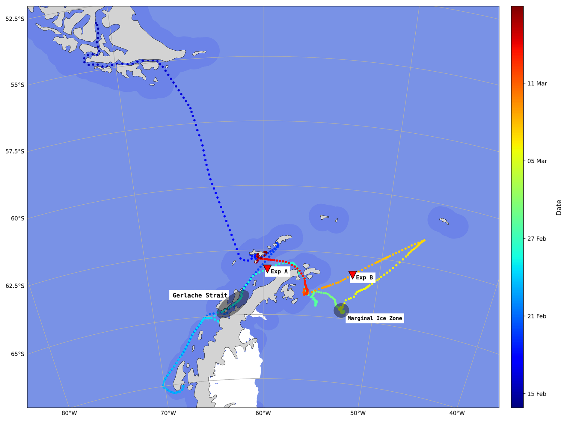
Figure 1 POLAR-CHANGE cruise track and location of the A and B ASIT experiments. The track colour (colour bar) indicates the sampling period, each point is the hourly position of the ship and the darker blue areas in the background indicate 100 km distance from the coast. Red triangles indicate the sampling location of each experiment. Transparent grey area refers to specific locations discussed in the text. The journey along the west coast of the Antarctic Peninsula was a round trip between the 21 and 26 February 2023.

Figure 2 ASIT experimental set-up in the POLAR-CHANGE cruise (as in Sellegri et al., 2023).

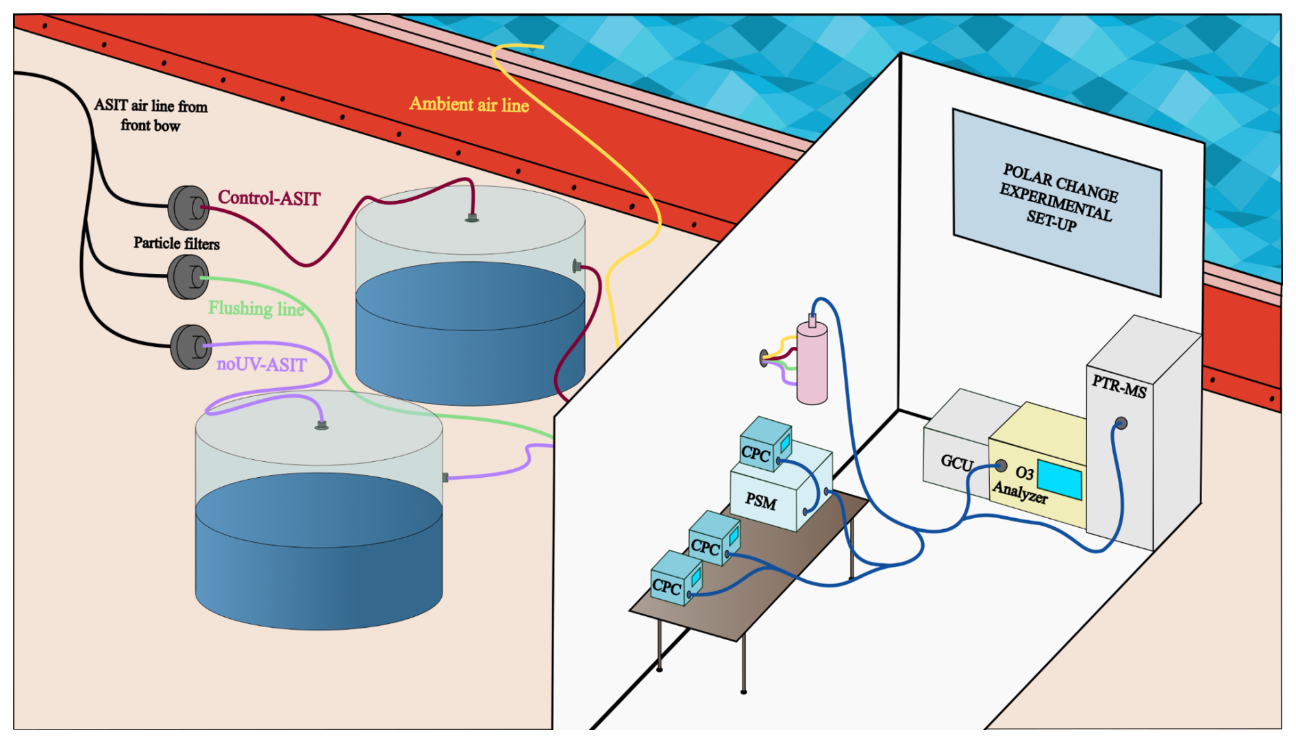
The experimental setup was similar to that described in Sellegri et al. (2023). It consisted of two Air-Sea Interface Tanks (ASITs) installed on deck and connected to a set of air analysis instruments installed in a container close to the tanks (detailed description below) (Fig. 2). The tanks, with a total volume of 1.8 m³, were half-filled with seawater pumped to the ASITs from a 4 m depth (see details below). A continuous flow of clean aerosol-free air at 25 L min⁻¹ was introduced into each of the ASITs via a flushing line, resulting in a residence time of 40 min. The outflows from the ASITs (purple and red lines, Fig. 2) were connected to the analytical instruments set via a four-way valve that switched every 20 min, allowing alternate measurements of the air from both ASITs, as well as the incoming air (from the flushing line; green line, Fig. 2), and the ambient air (yellow line, Fig. 2). During the POLAR-CHANGE cruise, one ASIT was covered with a lid transparent to all radiation wavelengths (Control-ASIT), while the other was covered with a lid blocking UV wavelengths below 380 nm i.e. removing UV light exposure inside the ASIT (noUV-ASIT) (Fig. S1 in the Supplement).

The ASIT headspace was continuously flushed with particle-free (filtered) air. In contrast, the lower section containing seawater was operated either in a continuous flow mode or in a static mode without water renewal. The continuous flow mode was used during most of the cruise with seawater being continuously pumped to the ASITs from a 4 m depth and flushed out with an average water residence time of approximately 6 h. This water continuous flow line supply is located 4–5 m below sea level, and consists of an epoxide-free silicone pipe connected to a centrifugal pump (BKMKC-10.11, Tecnium) in which the parts in contact with the fluid are made of polypropylene and glass. The pumping system is designed to be gentle and non-toxic to microorganisms and provide an uncontaminated continuous source of near-surface seawater. Simultaneous measurements of Chl a and DMS concentrations from the underway (UW) pumping system and a dedicated Go-Flo launched overboard, or the uppermost bottle from a conductivity, temperature and depth (CTD) cast have been compared during a previous cruse, and are in very good agreement (Royer et al., 2014). The static flow mode was applied in the two Experiments, A and B, in which the water remained incubated in the ASITs for 2 d.

To characterize the seawater entering the ASITs in continuous flow mode, samples were collected from the ship's underway water outlet on deck every 6–12 h (i.e. 2 to 4 times per day) throughout the entire cruise. This outlet was derived from the same intake water used to fill the ASITs. During experiments A and B, discrete water samples were also collected every 6 h from inside the ASITs (using a tap designed for this purpose), to monitor biological changes in the enclosed natural communities and to identify potential effects from UV light exposure. Cell abundances of microbial groups were estimated by combining flow cytometry and optical and fluorescence microscopy (described below).

2.2 Headspace characterization

The outgoing air line from the ASITs was connected to a set of instruments. An Ozone Analyzer (Thermo Scientific Model 49i) was used to monitor ozone. A Proton Transfer Reaction Quadrupole Mass Spectrometer (PTR-QMS, Ionicon) was used for VOC concentrations including DMS and MeSH. It was operated in standard conditions (Table S1 in the Supplement) and provided a $E/N$ ratio of about 130 Td (with E the electric field strength and N the gas number density, 1 Td = 10⁻¹⁷ V cm⁻²). Table S2 gives the $m/z$ monitored during the campaign, with the tentative name of the corresponding compound. As the mass resolution of the PTR-QMS is unit mass, we cannot rule out that interfering compounds were detected at the same $m/z$. However, the very good correlations found between MeSH concentrations and DMS concentrations, and between sea–air MeSH fluxes and DMS fluxes (Fig. 5), give good confidence to the mass attribution to the target compounds. A Gas Calibration Unit (Ionicon) was used for daily background instrument determination (catalyzer heated at 350 °C) and calibration. Three calibrations with an NPL (National Physics Laboratory, Teddington, UK) standard (including DMS) were made on-board and showed good stability of the instrument. Average instrument sensitivity for the different compounds is presented in Table S2. The Minimum Limit of Detection (MLD) was determined from the standard deviation of blank measurements, following the method described in Rocco et al. (2025b).

Sea–air fluxes in the ASITs were calculated based on the difference in concentration between the flushing air and the ASIT outflow, using the following equation:

$$\begin{array}{}\text{(1)}& F_{\text{ASIT-x}}=Q\times {\displaystyle \frac{C_{\text{ASIT}}-C_{\text{flush}}}{A}}\end{array}$$

where F_ASIT-x ($\mathrm{mol}{\mathrm{m}}^{-\mathrm{2}}{\mathrm{s}}^{-\mathrm{1}}$) is the net flux of the compound from the water to the air, Q (m³ s⁻¹) is the air volume flow rate in the ASITs, C_ASIT (mol m⁻³) is the concentration of the compound in the air leaving the ASIT, C_flush (mol m⁻³) is the concentration in the flush air entering the ASIT. A (m²) is the water surface area in the ASIT. Using comparisons between measured fluxes and their prediction from empirical relationships using measured seawater dissolved DMS concentrations, SST and windspeed, Rocco et al. (2025b) calculated that the ASIT system generated fluxes equivalent to open ocean 2 m s⁻¹ wind speed fluxes.

Particle concentrations were measured using several Condensation Particle Counters (CPCs), including two from TSI (Models 3010 and 3772) and a water CPC (MAGIC 200/210, Aerosol Devices). A Particle Size Magnifier (PSM, Airmodus A11) coupled to a CPC was also used in stepping mode. The particle counters provided concentrations with four cutoff diameters: 1 and 3 nm using the PSM, 5 nm using the MAGIC CPC, and 10 nm using the TSI CPCs. Loss corrections in the tubing were calculated according to the equation from Willeke and Baron (1993). The correction for the concentration of 1–3 nm particles (N_1–3) was made by considering an average diameter of 2 nm, and for 1–10 nm particles (N_1–10), by taking an average diameter of 3 nm. According to our analyses of the particle size distribution, this correction results in a slight overestimation of losses, which are generally smaller than estimated here. The formation rate of new particles was calculated with the following equation:

$$\begin{array}{}\text{(2)}& J={\displaystyle \frac{\mathrm{d}{C}_{\text{ASIT}}}{\mathrm{d}t}}-{\displaystyle \frac{Q\times C_{\text{flush}}}{V}}\end{array}$$

where J ($\mathrm{particles}{\mathrm{m}}^{-\mathrm{3}}{\mathrm{s}}^{-\mathrm{1}}$) is the rate of formation of new particles, C_ASIT (particles  m⁻³) is the concentration of particles in the air exiting the ASIT and C_flush (particles m⁻³) is the concentration of particles in the flushair entering the ASIT. Yet, the contribution of the second term, which corresponds to the contribution of particles entering the ASITs, is minimal due to the use of a particles filter on the flushing line. In the calculations of formation rates in the following sections, the concentrations taken will be those of particles greater than 1 nm (N₁) corrected for diffusion losses in the lines. t is time in seconds, Q (m³ s⁻¹) is the inlet flow into the ASITs in and V (m³) is the volume of the headspace in the ASITs.

The flushing air line for the ASITs was sourced from the bow of the vessel to avoid contamination from engine and kitchen exhausts as the ship moved forward. Data from the air lines were filtered for two hours after contamination events, which were identified based on elevated levels of ozone, benzene, and xylene, as well as changes in particle size distribution (N₁₀ > 0.5 × N₁) and variability in particle concentration during a 20 min measurement period.

Seawater concentrations of DMS in the ASIT (DMS_w) are calculated from headspace concentrations by using an average departure to the thermodynamical equilibrium, and therefore are more uncertain than direct measurements, as shown by offsets of the calculated values against the measured ones in the underway (Fig. S7). This departure to the thermodynamical equilibrium is based on the excellent correlation between the theoretical seawater concentrations calculated from the equilibrium with the headspace concentrations in the run-through mode of the control ASIT, and the measured concentrations in the underway seawater by Wohl et al. (2026). The slope of the measured versus calculated seawater concentrations was found to be 2.6 for DMS and 7.2 for MeSH. The slope found in the present study for DMS is very similar to the one used in Rocco et al. (2025b) that used the same experimental procedure (MeSH_w concentration was not measured in this previous study). Therefore, DMS_w was calculated using:

$$\begin{array}{}\text{(3)}& {\text{DMS}}_{\mathrm{w}}={\text{DMS}}_{\text{air}}\times f_{\text{sal}}\times H_{\mathrm{s}\left(T\right)}^{\text{cc}}\times \mathrm{2.6}\end{array}$$

where f_sal is a dimensionless factor accounting for the effect of salinity on solubility (f_sal = 0.848 for DMS, determined experimentally by Dacey et al., 1984) and 2.6 is the deviation from Henry's law equilibrium. $H_{\mathrm{s}\left(T\right)}^{\text{cc}}$ is the dimensionless Henry's law solubility expressed as concentration in water over concentration in air and is a function of temperature (T) (Sander, 2023).

2.3 Seawater biological parameters

• Chlorophyll a. Between 200 and 750 mL of seawater were filtered through 25 mm Whatman GF/F glass fibre filters. All filters were stored at −20 °C until analyses on board the R/V Hesperides. Chlorophyll a concentrations were estimated fluorometrically after extraction in 90 % acetone at 4 °C for 24 h (Yentsch and Menzel, 1963). Readings were conducted on a Turner 10AU fluorimeter calibrated with pure chlorophyll extract from spinach (Sigma C5357) using a Beckton-Dickinson spectrophotometer.

• Viral Abundance. Seawater subsamples (2 mL) were fixed with glutaraldehyde (0.5 % final concentration), kept at 4 °C for 15–30 min in the dark, flash-frozen in liquid nitrogen and finally stored at −80 °C until analysis, as described in Brussaard (2004). Viral counts were conducted in a Cytoflex flow cytometer at the ICM-CSIC laboratory (up to 5 months after sampling). Samples were diluted with TE-buffer (10:1 mM Tris: EDTA), stained with 50× SYBR Green I to a final concentration of 1 %, heated in an 80 °C bath for 10 min and run at a constant flow rate of 60 µL min⁻¹ according to Brussaard (2004). Viruses were determined using bivariate scatter plots of green fluorescence of stained nucleic acids versus side scatter (Brussaard, 2004). Antarctic waters often contain a high proportion of nucleocytoplasmic large DNA viruses (NCLDVs or “giant viruses”), especially during blooms of haptophytes, prasinophytes and cryptophytes. The cytometric settings used here follow standard protocols for marine viral enumeration and are consistent with studies from the Southern Ocean (Evans et al., 2009). These settings capture both small and large viral groups, as fluorescence intensity – rather than side scatter – reflects viral genome size and nucleic-acid staining (Brussaard, 2004; Evans et al., 2009). Thus, they are not expected to underestimate larger viruses. Based on green fluorescence and side scatter, we distinguished three viral populations (V1–V3), and a fourth (V4) in some samples, as in Vaqué et al. (2025). V1–V2 are typically dominated by bacteriophages (Biggs et al., 2021), whereas V3–V4 generally comprise eukaryotic algal viruses (Evans et al., 2009).

• Bacterial abundance. Seawater subsamples (2 mL) were fixed with 1 % paraformaldehyde + 0.05 % glutaraldehyde for bacteria estimations by flow cytometry. After 15–30 min in the dark at 4 °C, the fixed samples were flash-frozen in liquid nitrogen and subsequently stored at −80 °C. Bacterial abundances (Gasol and Del Giorgio, 2000) were measured in a Cytoflex flow cytometer at the ICM-CSIC laboratory (up to 5 months after sampling). On the day of analysis, samples were thawed, stained with 50× SYBR Green I at a final 1 % concentration and incubated for 5 min in the dark. Based on the flow cytometer side scatter versus green fluorescence (FL1) signatures, with high nucleic acid (HNA, considered active) from low nucleic acid (LNA, comparatively less active or dormant) content bacteria were identified.

• Pico-and nanophytoplankton abundance. Samples for photosynthetic pico- and nanophytoplankton abundances were collected on 5 mL cryovials, fixed with glutaraldehyde (1 % final concentration) and frozen in liquid nitrogen for cell enumeration by Flow Cytometry following Vaulot et al. (1989). Cell abundances were detected with a 488 nm laser beam from their signatures in a plot of side scatter (SSC) versus green fluorescence (FL3), separating the picophytoplankton fraction of 1–2 µm (sphere equivalent diameter, SED), the nanophytoplankton fractions of SEDs of 2–7, 7–15, 15–20 µm and the cryptophytes size classes (Cryptomonas spp., identified by their phycoerythrin signal in the FL3 vs orange fluorescence FL2 plots).

• Microplankton abundance. Some samples for the characterization of the microplankton (20–200 µm cell size; mainly diatoms and dinoflagellates) community were collected from the underway system (Rocchi et al., 2025) during the period when the ASIT experiments were run. Unfortunately, the samples were not collected consistently to track the changes inside the ASIT and can only provide a rough idea of the microplankton taxa in the seawater during the POLAR CHANGE cruise. This does not allow us to take into account the contribution of microplankton to VOC emissions and the links to new particle formation. Samples were processed using the Utermöhl method in 125 mL neutral Lugol fixed seawater (Edler and Elbrachter, 2010) and are presented in detail in Rocchi et al. (2025).

• Nanoflagellate abundance. Abundances of heterotrophic and phototrophic nanoflagellates, including Phaeocystis spp., in the size fraction 2–20 µm (SED) were determined by epifluorescence microscopy (Olympus BX40-102/E at 1000X). Subsamples of 30 mL were taken from seawater, fixed with glutaraldehyde (1 % final concentration), filtered through 0.6 µm black (25 mm diameter) polycarbonate filters, and stained with 4,6-diamidino-2-phenylindole (DAPI) at a final concentration of 5 µg mL⁻¹ (Sieracki et al., 1985). Counts of heterotrophic nanoflagellates (HNFs) and phototrophic nanoflagellates (PNFs) were conducted using an UV excitation filter (BP 360–370 nm) and barrier filter (BA 420–460 nm) and with a blue wavelength excitation filter (bandpass (BP) 460–490 nm) and barrier (emission) filter (BA; 510–550 nm). PNFs were distinguished under the blue light by the observation of red fluorescence emitted by photosynthetic plastid structures. At least 50 HNFs and 50 PNFs were counted per sample (3 transects of 5 mm in each filter) and classified into ≤ 2, 2–5, 5–10, and 10–20 µm size (SED) classes.

• Photosynthetic efficiency. The relative efficiency of excitation energy captured by the photosystem II (PSII), calculated as $F_{\mathrm{v}}/F_{\mathrm{m}}$, is used as a proxy of phytoplankton stress and fitness (Gorbunov et al., 2020; Gorbunov and Falkowski, 2022). The metric is measured by a multi-color fluorescence induction and relaxation instrument (mini-FIRe) (Gorbunov et al., 2020). The instrument records two parameters: F₀ as the minimal yield of fluorescence before fast light flashes, and F_m, the maximum yield of fluorescence due to the reradiation of the maximum number of photons. The difference between F_m and F₀ is called variable fluorescence (F_v). The quotient of $F_{\mathrm{v}}/F_{\mathrm{m}}$ represents the effective photosynthetic efficiency of the community measured under light conditions (Gorbunov and Falkowski, 2022). $F_{\mathrm{v}}/F_{\mathrm{m}}$ has no units, so that it is independent of the phytoplankton abundance and allows comparisons between environments, higher $F_{\mathrm{v}}/F_{\mathrm{m}}$ values indicates a better photosynthetic efficiency. Aliquots of 10 mL were sampled from the underway system and the ASITs and rapidly placed in the chamber of the mini-FIRe to apply the induction and relaxation protocol for dilute samples. No dark acclimation period was used. A hundred acquisitions were averaged for each sample using the fview software and the resulting data was processed with the fprope software to obtain all the desired parameters.

2.4 Statistical analysis

Statistical tests were performed using Python (version 3.11) with the SciPy library (version 1.16.2; Virtanen et al., 2020) at a significance level of α = 0.05. For paired measurements, normality of paired differences was first assessed with the Shapiro–Wilk test; when normality was not rejected, the paired t-test was applied, otherwise the non-parametric Wilcoxon signed-rank test was used, with effect size quantified by the rank-biserial correlation coefficient r. For independent, non-concurrent measurements, normality was assessed for each group separately, the Welch's t-test was applied when normality held for both groups and otherwise the Mann–Whitney U test was used, with effect size similarly quantified by the rank-biserial correlation coefficient r. When multiple comparisons were performed on the same variable, p-values were adjusted using the Bonferroni correction to control the family-wise error rate. For the correlation matrices, p-values were instead adjusted using the Benjamini-Hochberg false discovery rate procedure (Benjamini and Hochberg, 1995).

3 Results

3.1 Gas-phase concentrations and air–sea fluxes in the ASITs

Out of the 22 compounds monitored by the PTR-QMS, only two, DMS and MeSH, were found to be enriched in the ASITs headspace with respect to the entering flushing air. No enrichment of benzene, toluene, ethylbenzene and xylene (BTEX), monoterpenes, isoprene, or iodomethane were detected in the ASITs headspace, as the same molar fractions were observed at the inlet (i.e., in the flushing line) and the outlet (typically 0.13, 0.057, 0.05, and 0.1 ppb, respectively), differing from previous observations using this set-up with different seawaters (Rocco et al., 2021, 2025a). The most plausible explanation for the lack of emissions would be a subsaturation of these compounds in the water phase. For example, isoprene mean ambient atmospheric concentrations were around 50 ppt (Williams, 2026) and mean oceanic concentrations (UW) were 0.07 nM according to the measurement made during the campaign that are presented in Crabeck et al. (2026). They also present concentrations reaching 1.5 nM in top sea-ice, this could therefore be one of the sources of isoprene in the atmosphere that was identified as missing in the study by Ferracci et al. (2024). However, we cannot rule out the possibility of losses or heterogeneous reactivity in the ASIT's headspace that might mask emissions of BTEX or isoprene, but that would mean that emissions of these compounds are particularly low given the measurements taken during a previous campaign using the same set-up (Rocco et al., 2021, 2025b).

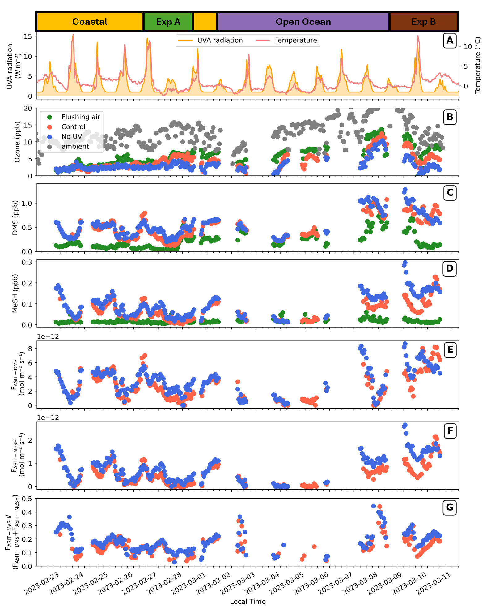
Figure 3 Time series of gaseous mole fractions and sea–air fluxes of DMS and MeSH, and the $F_{\text{ASIT-MeSH}}/(F_{\text{ASIT-DMS}}+F_{\text{ASIT-MeSH}})$ ratio within the ASITs over the cruise. Dates are noted in the x axis at the bottom of the figure, and the measurement phases of the cruise are indicated at the top. (A) Solar UVA radiation and ambient air temperature. (B) Ozone mole fractions in the ambient, flushing air, and the two ASITs outflow air. (C) DMS and (D) MeSH mole fractions in the flush and ASIT outflow air. The sea–air fluxes of DMS and MeSH as well as their ratio in the ASITs (Control and no UV) are shown in (E), (F) and (G), respectively. Symbols in (B) to (G) are as in legend inside (B).

Ozone mole fractions in the ambient air varied between 5 and over 20 ppb (Fig. 3) throughout the cruise with an average around 15 ppb. In contrast, ozone concentrations in the flushing line and the ASIT outlets were significantly lower, averaging around 7 ppb, primarily due to losses along the sampling line from the bow of the vessel (see Materials and methods). Notably, ozone levels in the ASITs were consistently lower than those in the flushing air, indicating further chemical reactions within the ASITs headspace or aqueous phase, that were estimated to contribute equally to ozone losses in a previous study (Salignat et al., 2026).

ASIT DMS and MeSH mole fractions and sea–air fluxes exhibited substantial variability over the cruise (Fig. 3). For the Control-ASIT (effect of UV filtering will be discussed Sect. 3.3) (Fig. 3E, red markers), the F_ASIT-DMS was on average 3.03 $\mathrm{pmol}{\mathrm{m}}^{-\mathrm{2}}{\mathrm{s}}^{-\mathrm{1}}$ (i.e., 0.26 $\mathrm{\mu }\mathrm{mol}{\mathrm{m}}^{-\mathrm{2}}{\mathrm{d}}^{-\mathrm{1}}$), peaking at 8.68 $\mathrm{pmol}{\mathrm{m}}^{-\mathrm{2}}{\mathrm{s}}^{-\mathrm{1}}$ on 10 March, while the average F_ASIT-MeSH was 0.64 $\mathrm{pmol}{\mathrm{m}}^{-\mathrm{2}}{\mathrm{s}}^{-\mathrm{1}}$ (i.e., 0.06 $\mathrm{\mu }\mathrm{mol}{\mathrm{m}}^{-\mathrm{2}}{\mathrm{d}}^{-\mathrm{1}}$), with a maximum of 2.65 $\mathrm{pmol}{\mathrm{m}}^{-\mathrm{2}}{\mathrm{s}}^{-\mathrm{1}}$ coinciding with that of F_ASIT-DMS. Note that fluxes of both compounds were always positive, i.e., these species were always degassing from seawater. Corresponding average seawater concentrations (Fig. S2) estimated for DMS (DMS_w) was 1.8 nM, reaching a maximum of 4.5 nM, while estimated MeSH_w averaged 0.8 nM, with a peak of 3.2 nM in the Control-ASIT (Fig. S2).

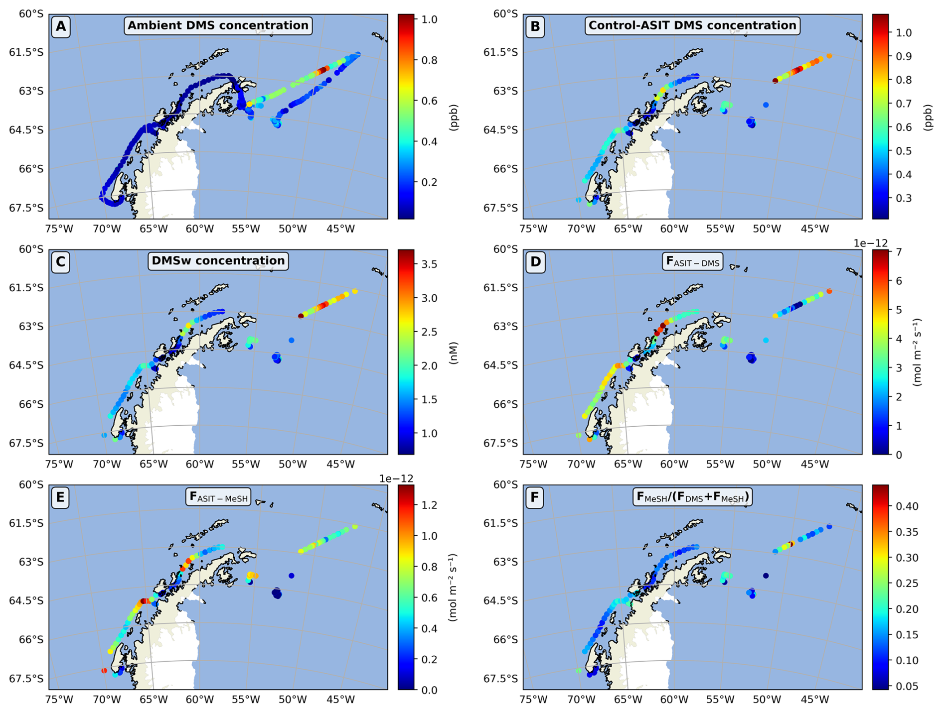
Figure 4 Ambient air DMS mole fraction (A) compared to ASIT air DMS mole fraction (B), estimated aqueous DMS concentration (C), DMS sea–air flux (D), MeSH sea–air flux (E), and the ratio of MeSH flux to DMS plus MeSH fluxes (F) in the Control–ASIT over the cruise.

The spatial variability of gaseous DMS molar fractions, estimated aqueous concentrations and sea–air fluxes in the Control-ASIT are shown in Fig. 4. As expected, aqueous DMS concentrations showed the same spatial variability as the gaseous DMS concentrations, with maxima measured in the open Southern Ocean north-east of the Antarctic Peninsula (2.5–3 nM) and minima in the Marginal Ice Zone (MIZ) (1 nM) as well as in the Gerlache Strait (< 1 nM) (location indicated in Fig. 1), which was characterized by lower salinity, reflecting the inflow of fresh water from melting ice. This low salinity trend in the Gerlache Strait was confirmed twice during the ship's outward and return passages through this area. Aqueous DMS concentrations along the west coast of the Antarctic Peninsula (2.5–3 nM) were moderate (around 1.5–2 nM). Ambient air DMS molar fractions (Fig. 4A) were also higher in one open-ocean transect north of the Weddell Sea (0.4–1 ppb) than over most of the rest of the cruise track (< 0.3 ppb). Ambient air concentrations are a function of local fluxes from the ocean, but are also contributed by emissions upwind. Thus, matching observed atmospheric concentrations and emission fluxes is not straightforward. In addition to seawater concentrations, sea–air fluxes in the ASITs are, by definition, a function of incoming ambient air DMS concentrations; therefore, they showed a pattern which is different from that of estimated aqueous DMS concentrations. Fluxes can be low despite high seawater concentrations when incoming gaseous concentrations in the flushing air are high, as occurred over a portion of the transect north of the Weddell Sea. Conversely, fluxes were particularly high in coastal waters to the west of the peninsula, where DMS concentrations in the ambient air were particularly low. Air concentrations, estimated aqueous concentrations and sea–air fluxes of MeSH in the ASIT showed patterns parallel to those of DMS. The ratio of MeSH flux to the sum of sulfur compound fluxes varied from 0.1 to 0.2 for most of the data (Figs. 4F and 6A). Causes of this variability will be further addressed in the following sections.

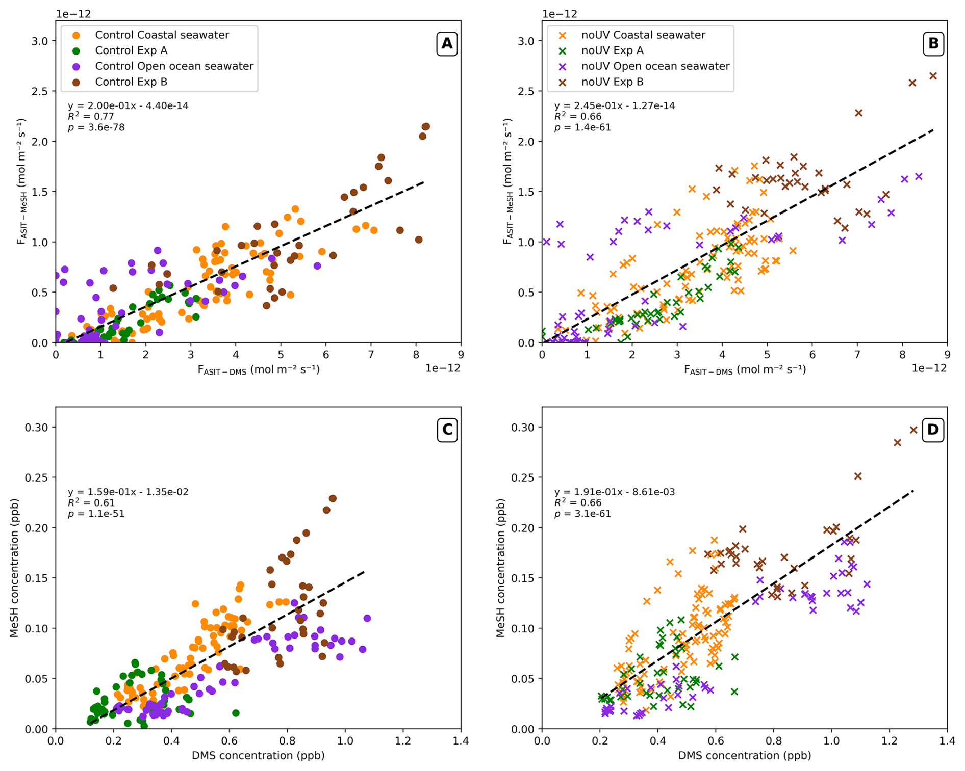
Figure 5 Relationship between hourly averaged DMS and MeSH sea–air fluxes (A, B) and air molar fractions (C, D) in the Control (lefthand plots) and noUV (righthand plots) ASIT with the associated equation, R² and p-value. Colour indicates measurement periods in the coastal and open ocean.

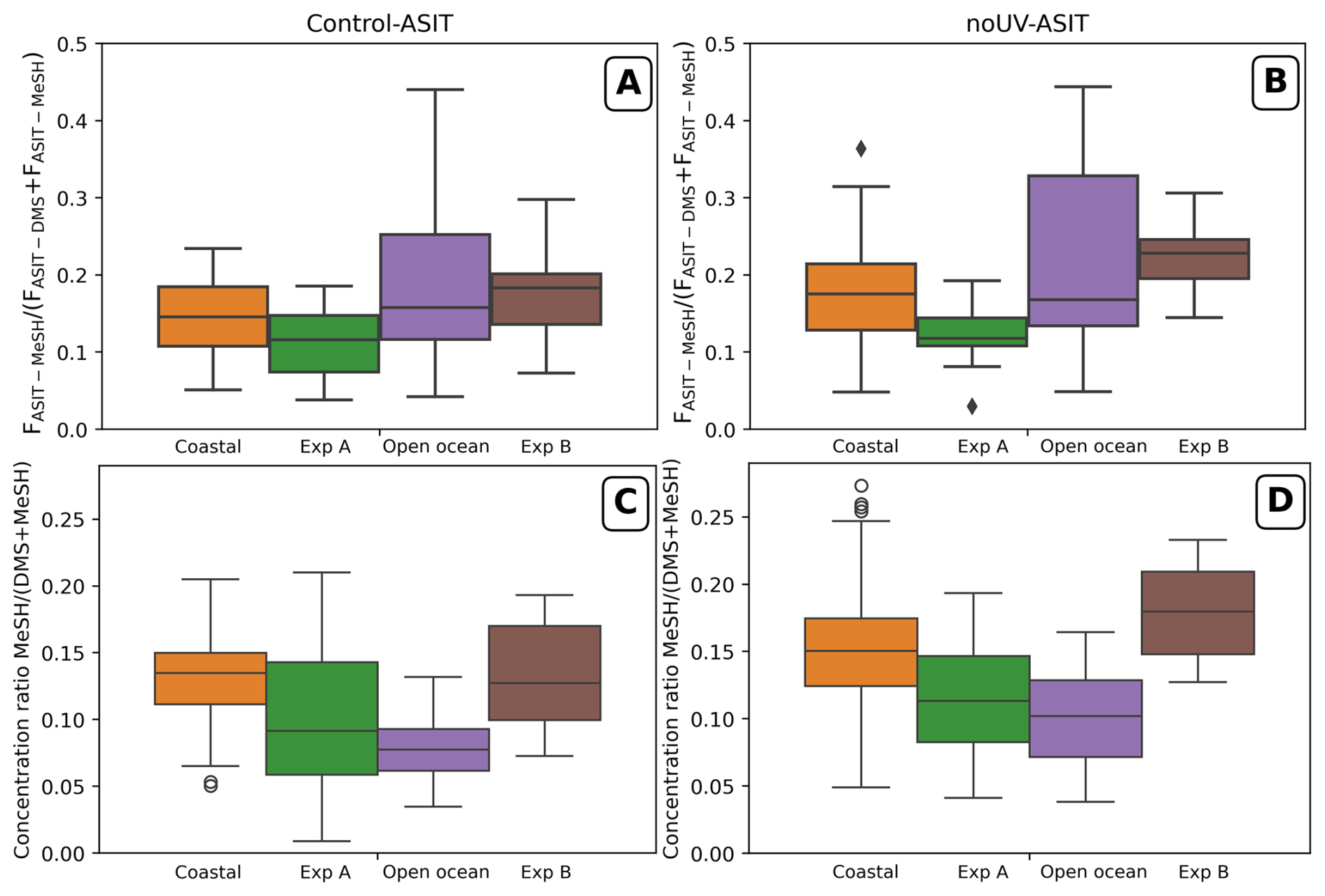
Figure 6 Boxplot of the $F_{\text{ASIT-MeSH}}/(F_{\text{ASIT-DMS}}+F_{\text{ASIT-MeSH}})$ ratio (A, B) and the air concentration ratio (C, D) for each observational period in the Control (lefthand plots) and noUV (righthand plots) ASIT. Boxes represent the interquartile range (IQR, 25th–75th percentiles), horizontal lines the median, whiskers extend to 1.5× IQR, and outliers are plotted as points.

A strong correlation was observed between sea–air MeSH and DMS fluxes in both ASITs, with R² values of 0.77 for the Control-ASIT and 0.66 for the noUV-ASIT, across all coastal and open ocean measurement periods (Fig. 5A and B). The median value of the F_ASIT-MeSH $/$ (F_ASIT-DMS+F_ASIT-MeSH) ratio obtained for all data combined was 0.17 (first quartile Q1 = 0.13; third quartile Q3 = 0.22) in the Control-ASIT (Fig. 6A). There do not appear to be major differences between the enclosed experiment periods and the periods with continuous water flow into the tanks, except that the ratio was less variable during the experiments, reflecting the more stable water composition in the ASITs. However, the average $F_{\text{ASIT-MeSH}}/(F_{\text{ASIT-DMS}}+F_{\text{ASIT-MeSH}})$ in Experiment B (with open ocean waters) was significantly higher than in Experiment A (with coastal water types) in Control-ASIT (Mann–Whitney U = 192, nexpA = 29, nexpB = 33, p = 5.46 × 10⁻⁵, r = 0.599) and in noUV-ASIT (Mann–Whitney U = 47, nexpA = 39, nexpB = 32, p = 2.70 × 10⁻¹¹, r = 0.925).

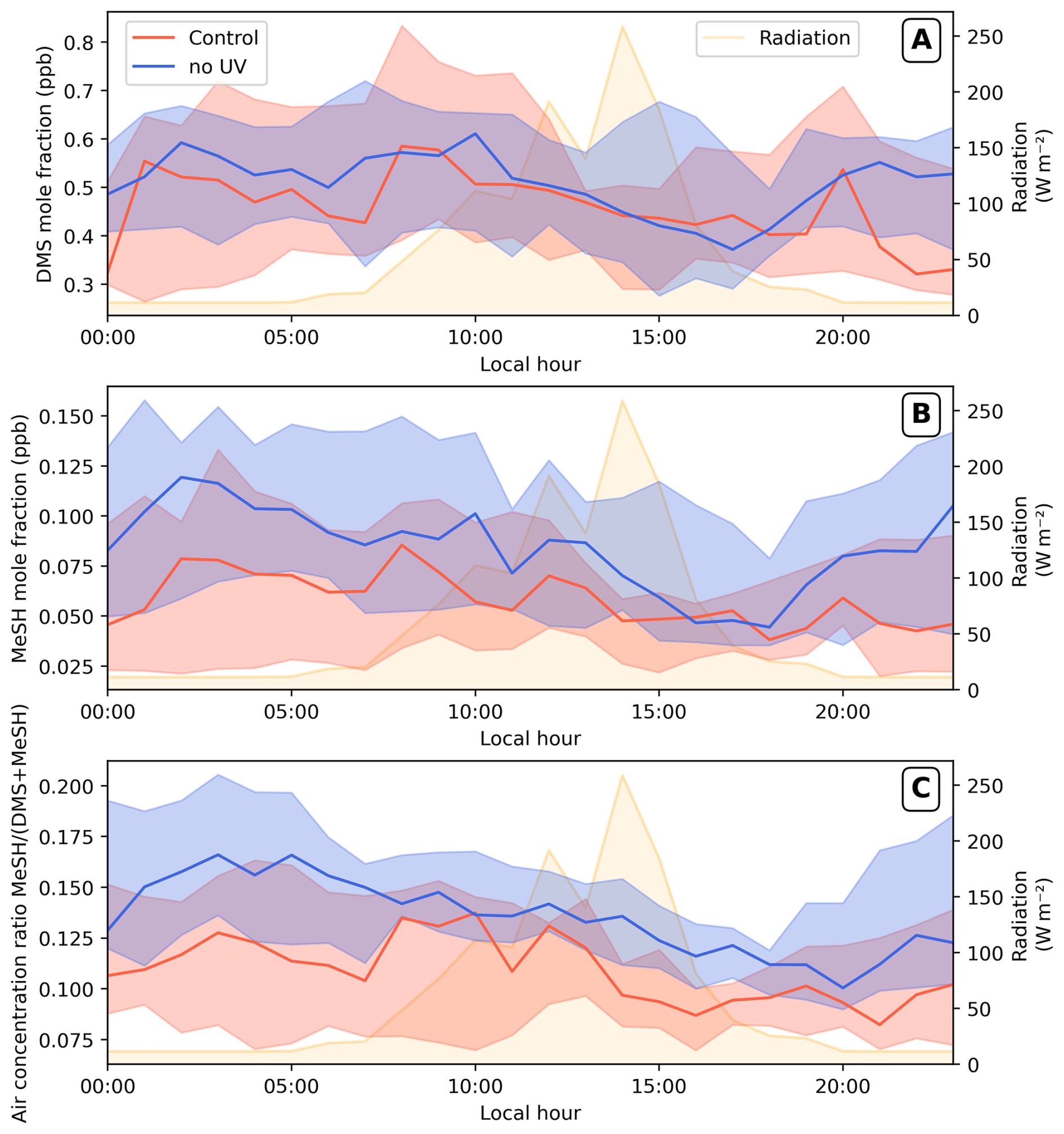
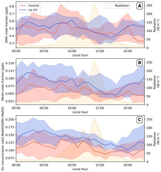
Figure 7 Median ± 1st and 3rd quartiles of the diel pattern of the gaseous DMS (A) and MeSH (B) mole fractions and their ratio (C) in both ASITs (Control, red; noUV, blue) considering all data over the entire cruise (i.e. from the measurement periods, including coastal, open ocean and Experiments A and B). Irradiation daily variation is indicated by the yellow area.

DMS and MeSH molar fractions both have a diel variation, stronger for MeSH than for DMS (Fig. 7). The diel variation of the DMS mole fraction appear clearly when the fractions are normalized to the daily maxima molar fraction (Fig. S5A) with a decrease between 12:00 and 19:00 LT and an increase of the molar fractions in the hours following the decline of radiation level, with significantly stronger diel contrast in the Control-ASIT (paired t-test, n = 193, t = −4.95, p = 1.6 × 10⁻⁶), most notably around midnight (00:00 LT: mean difference = 0.13 ± 0.12, r = 0.94, p = 0.016). The diel variation of MeSH molar fraction was even clearer with high fraction at night and decrease through the day (Figs. 7B and S5B). This pattern was marked in the noUV-ASIT both during day and night in molar fraction but is clearer for Control-ASIT when the fractions are normalized with significant differences (Wilcoxon signed-rank test, n = 193, W = 6118, p = 6.7 × 10⁻⁵, r = 0.35), particularly around 14:00 and 16:00 LT (r = 0.944 and 1.00, p < 0.05) (Fig. S5B).

3.2 New particle formation

The concentrations of 1–3 nm ($N_{\mathrm{1}--\mathrm{3}}$), 1–10 nm (N_1–10), > 1 nm (N₁) and > 10 nm (N₁₀) particles are presented in Fig. 8. The formation rates of 1 nm particles (J1) are obtained using the method presented in Sect. 2. In the Control-ASIT, very few and weak new particle formation events were observed (Fig. 8) with N₁ particle concentrations reaching up to 38 particles cm⁻³, mainly composed of 1 to 3 nm particles, and formation rates peaked at 0.02 $\mathrm{particles}{\mathrm{cm}}^{-\mathrm{3}}{\mathrm{s}}^{-\mathrm{1}}$. Few of these particles reached higher size than 10 nm which is consistent with the short residence time (40 min) in the ASITs. Most of the particles in the Control-ASIT were formed with coastal waters and new particles formation occurs only in the middle of the day, around maximum radiations periods (Fig. 9). The effect of filtering UV light on new particle formation will be addressed in the next section.

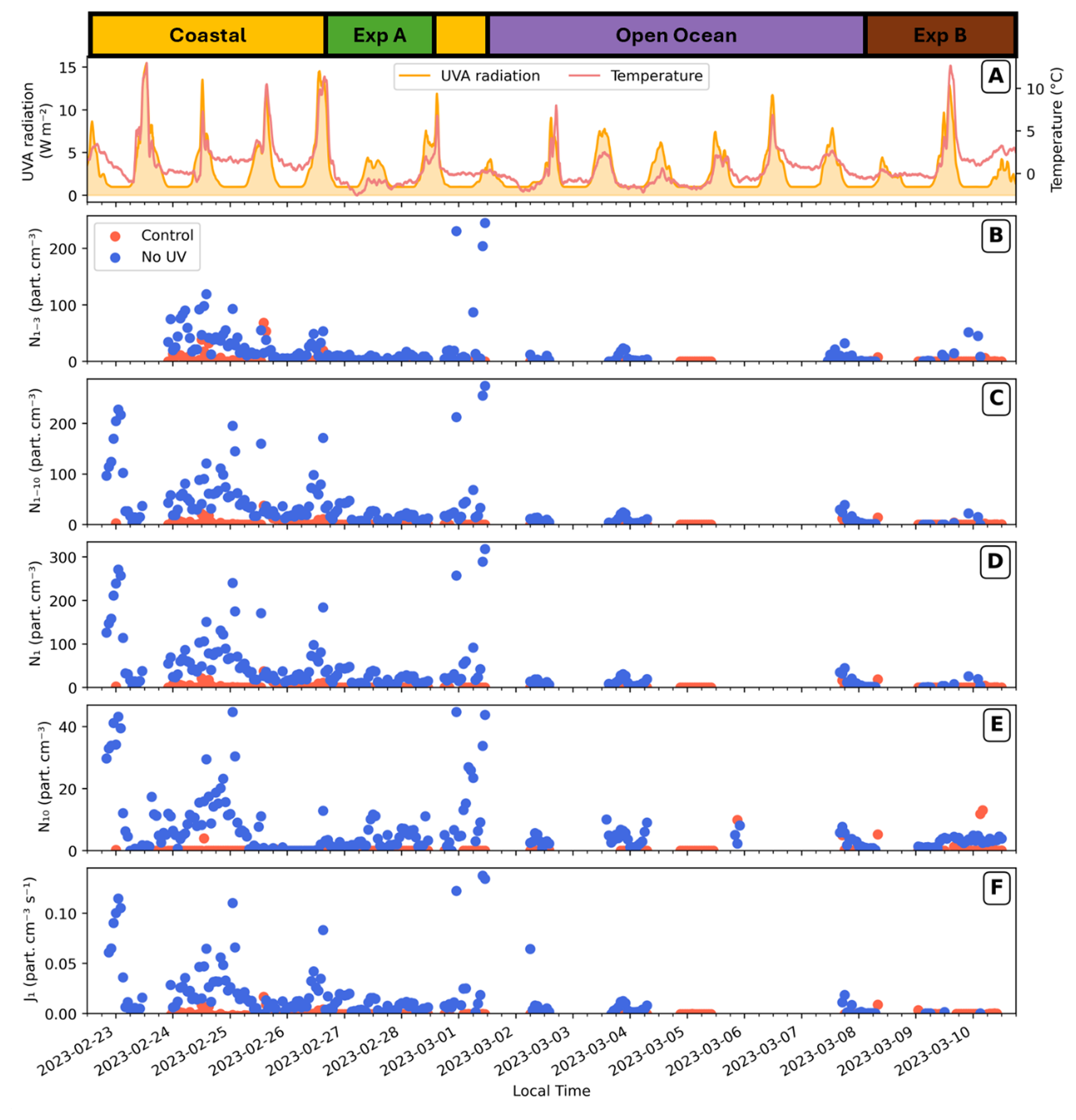
Figure 8 Time series of sized particle concentrations (B–E) and particle formation rates (F) in the ASITs. Air temperature inside the ASITs and solar radiation (UVA) are indicated (A) and measurements periods are presented on top of the figure.

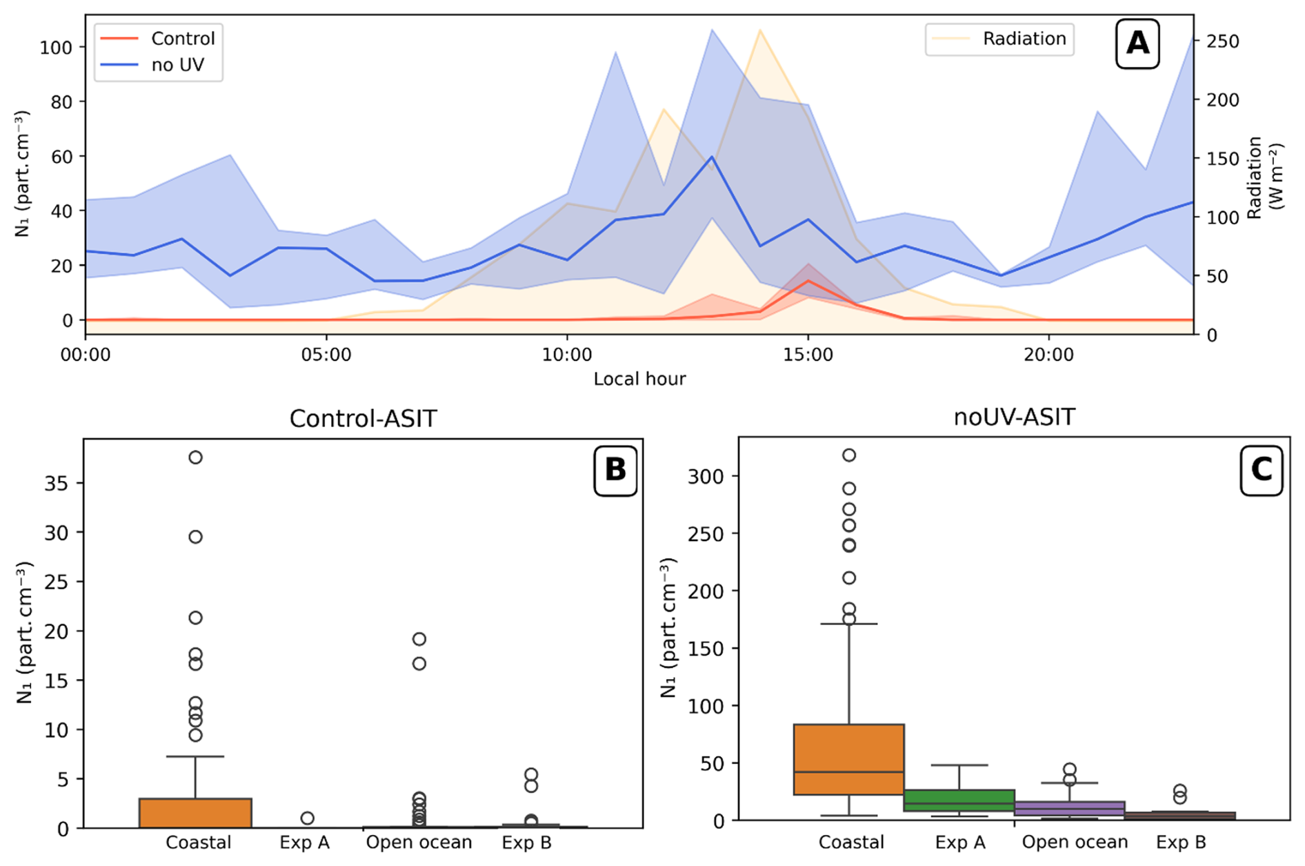
Figure 9 (A) Median diel profile of the N₁ particle concentration in the ASITs headspaces, all measurement periods merged (median ± 1st and 3rd quartile); irradiation daily variation is indicated by the yellow area. Boxplots of the N₁ particle concentration by seawater type within each ASIT headspace (B, Control; C, noUV) on different axis.

3.3 Differences induced by UV

3.3.1 DMS, MeSH and ozone concentrations

Sea–air fluxes and concentrations of DMS and MeSH were consistently higher in the noUV-ASIT than in the Control-ASIT (Figs. 3C, D and 7A, B). On average, DMS fluxes were 24 % higher and MeSH fluxes 58 % higher in the noUV-ASIT. The difference between ASITs is statistically significant (confirmed by a paired Wilcoxon signed-rank test) both for DMS (W = 4129, p-value = 1.66 × 10⁻¹¹, r = 0.56) and MeSH (W = 1698, p = 6.12 × 10⁻²³, r = 0.82) indicating a clear negative impact of UV-light especially on MeSH molar fractions (Fig. 7). These differences were even more pronounced during Experiment A and the beginning of Experiment B (Fig. 3). Decreased MeSH mole fractions in the presence of UV-light were observed during the experiments and also outside the experimental periods, while for DMS, the difference between the noUV-ASIT and Control-ASIT was noticeable mostly during experiments as for the sea–air fluxes (Fig. S3). Interestingly, the highest impact of UV, especially on MeSH concentrations, occurred during the night with increased concentrations when UV light was filtered out (Fig. 7B). This effect is also observed on DMS concentrations (Fig. 7A).

The median value of the $F_{\text{ASIT-MeSH}}/(F_{\text{ASIT-DMS}}+F_{\text{ASIT-MeSH}})$ ratio obtained for all data combined was slightly lower in the Control-ASIT (Median = 0.15; Q1 = 0.11; Q3 = 0.19) than in the noUV-ASIT (Median = 0.17; Q1 = 0.13; Q3 = 0.22) with a significant difference (W = 1025, p-value = 1.17 × 10⁻¹⁹, r = 0.835). This was also observed for the air concentrations ratios and calculated aqueous concentrations ratios with median values of aqueous concentrations of 0.27 (Q1 = 0.20; Q3 = 0.33) in the Control-ASIT and 0.32 (Q1 = 0.26; Q3 = 0.38) in the noUV-ASIT (significative: W = 1495, p-value = 4.38 × 10⁻²⁴, r = 0.840). Moreover, as illustrated in Fig. 7C, the decrease in the ratio of MeSH to DMS linked to UV light exposure was more pronounced. Finally, the MeSH–DMS relationship was more linear in the Control-ASIT and more scattered in the noUV-ASIT, both across and within different measurements periods (Fig. 5).

Outside the experimental periods, ozone levels differed only slightly between the two ASITs (Fig. 3B). In contrast, during Experiments A and B, clear differences emerged in the ASIT ozone concentrations. During Experiment A, the noUV-ASIT exhibited on average 38 % (± 17 %) lower ozone concentrations than the Control-ASIT (paired t-test, n = 40, t = 13.99, p < 0.001), and during Experiment B this difference increased to 50 % (± 16 %) (paired t-test, n = 35, t = 18.92, p < 0.001).

3.3.2 Aerosol particle concentrations and formation rates

Filtering out UV light had a large impact on the formation of new particles, which were observed in significantly higher concentrations in the absence of UV-light (Fig. 8) (Wilcoxon signed-rank test between both ASITs, W = 44, p = 1.20 × 10⁻²⁷, r = 0.993). N₁ particle concentrations reached up to 300 particles cm⁻³ in the noUV-ASIT, and J1 highest nucleation rates were close to 0.15 $\mathrm{particles}{\mathrm{cm}}^{-\mathrm{3}}{\mathrm{s}}^{-\mathrm{1}}$ (Fig. 8D and F, respectively). The highest particle concentrations were obtained with coastal waters (Fig. 9B) on both sides of the Antarctic Peninsula (Fig. S6). In contrast, particle concentrations with open ocean waters and both experiments were lower (Fig. 8B–E): 48, 45 and 26 particles cm⁻³ in the noUV-ASIT for Experiment A, open ocean waters, and Experiment B, respectively. Moreover, experiments A and B showed significantly lower particle concentrations than with their respective seawater outside of the experiments (Mann–Whitney U = 3336, n₁ = 96, n₂ = 42, p = 1.02 × 10⁻⁹, r = −0.655 for difference between coastal seawaters and exp B; and Mann–Whitney U = 299, n₁ = 41, n₂ = 10, p = 2.65 × 10⁻², r = −0.459 for difference between open ocean seawaters and exp B). Diel variations in N₁ particles (Fig. 9A) showed that most new particle formation in the noUV-ASIT occurred in the middle of the day or at night, with a decrease in formation rates at the beginning and end of the daylight period. Again, these diurnal variations of N₁ differ from previous observations performed in the ASITs in the Southwestern Pacific Ocean during the Sea2Cloud ship campaign, where N₁ were preferentially formed at the end of the night prior to dawn (Chamba et al., 2023).

3.3.3 Seawater microorganisms

In Experiments A and B, in general, the abundances of most pico-nanophytoplankton groups remained stable or increased, suggesting that they performed relatively well in the ASITs over the 48 h duration of the experiments (Figs. 10 and S4). Trends in chlorophyll a concentration, a proxy for the biomass of photosynthetic organisms, corroborates this finding, remaining stable during Experiment A and increasing during Experiment B (Fig. S4A and B). However, the different groups exhibited differing responses. The cell abundances of the biggest (15–20 µm SED nanophytoplankton, Fig. 10A and B) and smallest (< 2 µm SED, picoplankton, Fig. 10G and H) size fractions were higher in Experiment A (with incubated coastal seawater), while the 7–15 and 2–7 µm SED nanophytoplankton abundance (Fig. 10C–F) were similar or increased in some treatments during Experiment B (with open ocean water). Regarding the sensitivity to UV light, phytoplankton cell counts were significantly lower under UV exposure (Control-ASIT) than in the noUV-ASIT for the 1–2 µm picoplankton and for the 2–7 and 7–15 µm nanophytoplankton, both when experiments were analysed individually (Wilcoxon signed-rank test, n = 9; 1–2 µm: r = 1.00, p = 0.008 in both experiments; 2–7 µm: Exp A r = 0.91, p = 0.023, Exp B r = 0.87, p = 0.039; 7–15 µm: Exp A r = 0.87, p = 0.039, Exp B r = 1.00, p = 0.008) or with both experiment combined (n = 18; 1–2 µm: r = 1.00, p < 0.001; 2–7 µm: r = 0.88, p = 0.003; 7–15 µm: r = 0.97, p < 0.001). In contrast, the 15–20 µm nanophytoplankton size class showed no significant difference between treatments, suggesting that UV sensitivity was strongly size-dependent, with the smallest size classes being consistently and most strongly affected. In contrast, only cryptophytes experienced an apparent positive response to the UV light towards the end of Experiment B (Fig. S4) even though, in both experiments, UV light neither significantly favored nor disadvantaged the cryptophytes over the period considered.

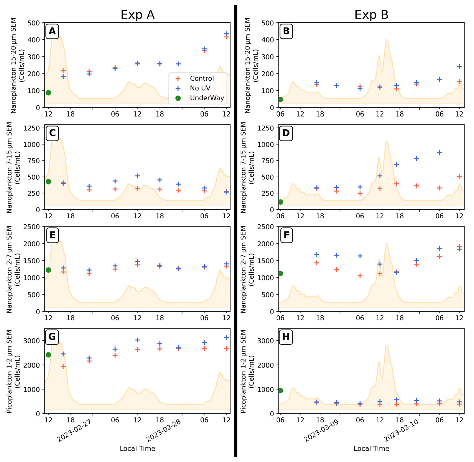
Figure 10 Evolutions of the 15–20 µm SED nanophytoplankton (A, B), 7–15 µm SED (C, D), 2–7 µm SED (E, F) and picoplankton 1–2 µm SED (G, H) abundances in both ASITs during Experiments A and B. The starting point (green filled circle) represents the measurement in the seawater sample from the underway inlet system at the beginning of the experiments and may not exactly reflect the initial water composition inside the ASITs. Irradiation daily variation is indicated by the yellow area.

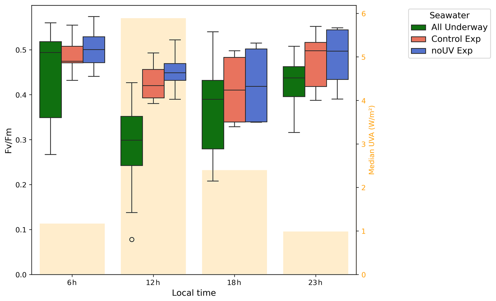
Figure 11 Diel $F_{\mathrm{v}}/F_{\mathrm{m}}$ variation in samples concurrently collected from the two ASITs during both experiments (Control exp and noUV exp) and from the underway water inlet during the whole POLAR-CHANGE campaign (All Underway). Median UVA radiation is indicated by yellow bars.

The $F_{\mathrm{v}}/F_{\mathrm{m}}$ ratio, a proxy of phytoplankton photosynthetic efficiency, showed a clear diel pattern, with lower median values during the day and higher values at night (Fig. 11). This pattern was consistent between the two ASITs and reflected the same diel variation observed in the seawater from the underway inlet measurements. However, $F_{\mathrm{v}}/F_{\mathrm{m}}$ values within the ASITs exhibited less variability throughout the day and were overall higher compared to the seawater from the underway system outlet, particularly around noon, with larger size effect in both ASITs compared to UW even with small sample size (Mann–Whitney U = 382, n₁ = 62, n₂ = 18, p = 0.043, r = 0.315) for Control-ASIT Exp; U = 326, n₁ = 62, n₂ = 18, p = 0.008, r = 0.417 for noUV-ASIT Exp). Therefore, higher photosynthetic efficiencies suggest a reduction in phytoplankton stress within the ASITs, especially at noon.

UV exposure did not seem to significantly impact phytoplankton photosynthetic efficiency as both Experiments A and B progressed, leading to marginally lower $F_{\mathrm{v}}/F_{\mathrm{m}}$ in the Control-ASIT by the end of the experiment period (Fig. S4G and H). UV light showed little impact on the bacterial concentrations except on the second day of Experiment B (Fig. S4F), where during a 12 h period UV impacted negatively on the low-DNA bacteria and positively on the HNA bacteria concentrations (Fig. S4D).

4 Discussion

4.1 Gas-phase emissions and reactivity

DMS and MeSH positive sea–air fluxes indicate emission from seawater linked to marine biological processes (Fig. 3). The equivalent wind speed inside the ASIT headspace was estimated as 2–3 m s⁻¹ (Rocco et al., 2025b), i.e., significantly lower than typical conditions at the ocean surface. Consequently, a comparison to ambient fluxes in the literature is not useful but a comparison to similar experiments performed in the Southwestern Pacific Ocean during the Sea2Cloud voyage can be done (Sellegri et al., 2023). In Sea2Cloud, the average DMS fluxes in the Control-ASIT were 23.2, 8.2, and 2.9 $\mathrm{pmol}{\mathrm{m}}^{-\mathrm{2}}{\mathrm{s}}^{-\mathrm{1}}$ (i.e. 2.0, 0.7 and 0.3 $\mathrm{\mu }\mathrm{mol}{\mathrm{m}}^{-\mathrm{2}}{\mathrm{d}}^{-\mathrm{1}}$) for frontal, subantarctic, and subtropical waters, respectively. The fluxes observed during POLAR-CHANGE (3.03 $\mathrm{pmol}{\mathrm{m}}^{-\mathrm{2}}{\mathrm{s}}^{-\mathrm{1}}$, peaking at 8.68 $\mathrm{pmol}{\mathrm{m}}^{-\mathrm{2}}{\mathrm{s}}^{-\mathrm{1}}$) were similar to Sea2Cloud fluxes in subantarctic and subtropical waters. Consequently, calculated aqueous DMS concentrations (0.3–4 and 1–4.3 nM for Control and noUV ASITs, respectively) were similar to those measured during the Sea2Cloud in subantarctic seawaters (3–5 nM; Rocco et al., 2025b).

During Experiments A and B, the estimated lower concentrations of DMS_w in the Control-ASIT (Fig. S2) are likely due to an aqueous-phase reactivity (loss) of DMS, which is accumulating over several days in static flow mode (Salignat et al., 2026) as opposed to the continuous flow mode. Indeed, the gas-phase photochemical loss of DMS was shown to be negligible within the 40 min residence time of our experimental set-up (Rocco et al., 2025b; Salignat et al., 2026). Salignat et al. (2026) also report that the diel profile observed for DMS in the ASIT incubated seawater during Sea2Cloud, with maxima during the night and minima during the day was explained by aqueous-phase ozonolysis when a constant (day and night) production was prescribed. Earlier, Brimblecombe and Shooter (1986) demonstrated the photooxidation of DMS in seawater under UV irradiation. Various studies have reported that photochemical degradation can account for 7 % to 40 % of dissolved DMS loss in the ocean (Galí et al., 2023), depending on regional conditions, and have linked these losses to oxidants produced by chromophoric dissolved organic matter (CDOM) and ${\mathrm{NO}}_{\mathrm{3}}^{-}$ photolysis when ${\mathrm{NO}}_{\mathrm{3}}^{-}$ concentrations are higher than 1 µM, as is the case in Antarctic waters (Bouillon and Miller, 2005). The hypothesis of aqueous-phase oxidation also provides a plausible explanation for the persistence of emission differences at night, when UV radiation is absent. Although the average residence time of the water in the ASITs was approximately six hours, the residence time in a continuously stirred reactor is a distribution of residence times with some parcels being expelled from the reactor before the six hours and some parcels having much longer residence time. This means that daytime chemical transformations in the water produce compounds that persist during nocturnal periods. Additionally, ozone-mediated oxidation of DMS in seawater, as discussed by Hoffmann et al. (2016) and Salignat et al. (2026), could contribute to the observed differences between the ASITs. Since ozone concentrations were generally higher in the Control-ASIT for most of the campaign, and the ozone differential between ASITs showed a weak anti-correlation with the differences in DMS and MeSH fluxes, this mechanism may play a role. Although aqueous oxidation of MeSH could also be enhanced under these conditions, this process remains poorly characterized in the literature. A different DMS production induced by UV stress such as DMSP production inhibition could also explain part of the differences between the ASITs.

A strong positive correlation was found in DMS and MeSH fluxes (Fig. 5), as also previously reported earlier by Novak et al. (2022) over non-enclosed coastal waters (R² = 0.65) and for molar ratio in previous ASIT measurements by Rocco et al. (2025b) (R² = 0.81 in the Control-ASIT). The literature, mainly recent, reports ratios of MeSH to total volatile methylated sulfur pools and fluxes close to those reported here, generally between 0.10 and 0.40. Gros et al. (2023) reported a ratio of $\mathrm{MeSH}/(\mathrm{DMS}+\mathrm{MeSH})$ concentrations in water averaging 0.20 in the North Atlantic but varying greatly with latitude and regularly reaching 0.40 above 70° N. Leck and Rodhe (1991) estimated the average ratio of $\mathrm{MeSH}/$ (sulfur species) in the Baltic and North Seas at around 0.07, based on concentrations in water and including CS₂ and dimethyl disulfide (DMDS) among the sulfur species. Lawson et al. (2020) calculated flux ratios of 0.14 to 0.24 in the Southwest Pacific, neglecting oxidative losses at night. A ratio value of 0.16 in dissolved concentration and 0.17 in fluxes was found by Kettle et al. (2001) in the South and North Atlantic. Finally, during the Sea2Cloud campaign, the $F_{\text{ASIT-MeSH}}/(F_{\text{ASIT-DMS}}+F_{\text{ASIT-MeSH}})$ ratio ranged between 0.11 and 0.18 in the Control-ASIT (Rocco et al., 2025b). Thus, the values obtained in the present study are consistent with previous measurements, with values mainly between 0.10 and 0.20, but reaching 0.30 to 0.45 mostly in open ocean waters. Air concentration ratios within the Control-ASIT headspace (median of 0.11; Q1 = 0.8; Q3 = 0.14) were in the range of those reported by Mynard et al. (2025), between their Antarctic Ice-Edge (median of 0.07) and the subtropical front region (0.11–0.15).

The diel pattern of MeSH concentrations showed a decrease in the afternoon, in both ASITs, that may mainly be resulting from the higher gas-phase OH-reactivity (or photochemical loss) of MeSH compared to DMS, within the 40 min residence time in the ASIT's headspace. Greater chemical loss for MeSH than for DMS would then be behind the observed diel variation of the air $\mathrm{MeSH}/(\mathrm{MeSH}+\mathrm{DMS}$) concentration ratio, as also suggested by Mynard et al. (2025), and could explain the significant differences in MeSH concentration between the two ASITs and a lower $\mathrm{MeSH}/(\mathrm{MeSH}+\mathrm{DMS}$) ratio during the day compared to night, even outside the experimental periods. These observations closely resemble the diel pattern reported by Novak et al. (2022). Lawson et al. (2020) reported broadly similar diel profiles for DMS and MeSH, with a production minimum around 4 p.m. (local time) for both compounds, a trend more evident for MeSH in our experiments. However, a closer look at our measurements reveals that the MeSH concentration differs from one ASIT to the other most at night, which points to the oxidation of MeSH in the Control-ASIT being from another oxidant than OH (i.e., a nighttime aqueous-phase oxidant at larger concentrations in the presence of daytime UV), or to an impact of UV on the biology processes leading to a change in the production of MeSH in the seawater at night.

The difference in ozone concentration between ASITs may be attributed to several factors, including chemical reactions with other gaseous species, interfacial reactions during the air residence time (∼ 40 min), or aqueous-phase reactions occurring over the 6 h water residence time. These ozone losses, which occasionally reached 100 % between the flushing air and ASIT headspace, were variable over time, suggesting that chemical reactivity, rather than physical deposition alone, played a significant role. If physical losses to surfaces were dominant, they would likely remain relatively constant or vary in relation to temperature. The noUV-ASIT lid blocked nearly all radiation below 375 nm (Fig. S1), preventing most photochemical processes. In the presence of NO, the photolysis of NO₂ and NO₃ (which requires wavelengths < 410 nm; Bower et al., 1993; Andersen et al., 2022) would be inhibited, potentially leading to a reduction in ozone production while ozone consumption continues unabated. One other potential explanation for the increased ozone losses in the noUV-ASIT is a higher ozone consumption, that could be due to enhanced water-to-air net fluxes of reactive compounds, particularly DMS and MeSH, whose fluxes were indeed higher in the noUV-ASIT during both experiments (see Fig. 3). It could also be the ozonolysis of organic matter, accumulated over time especially during experiments, potentially leading to more VOC emissions (Kilgour et al., 2024). The increased difference between ASITs in Experiments A and B suggests that UV removal had a significant impact on the aqueous-phase chemistry (as discussed earlier) that in turn impacts ozone losses to the aqueous phase during experiments. The temporal pattern of these changes also provides insight into the relevant timescales: the differences between the two ASITs emerged within the first 12 h of the experiments, reaching 37 % higher ozone in the Control-ASIT compared to the noUV-ASIT in Experiment A and 38 % in Experiment B at that time point. This indicates that reactions in the aqueous phase and associated emission processes occur over timescales longer than six hours, but less than 12 h in this experimental setup.

4.2 Links between dissolved gases and microorganisms during experiments

We explored the potential links among the different biological elements and chemical compounds measured in the ASIT experiments by considering the temporal patterns and the correlations between the different parameters (Figs. 12 and S8). Note that significant correlations should not always be interpreted as a direct cause-effect relationship, nor a short-term response occurring in the ASITs. Furthermore, the correlations should be taken individually, as indicators of the diverse, dynamic and complex biological processes undergoing in the ASIT experiments, somewhat apparently contradictory in some cases. In Experiment A, which involved incubating coastal water in the ASITs for 2 d, DMS and MeSH seawater concentrations slightly decreased over time, particularly in the Control-ASIT, where MeSH concentrations became almost zero, before rising up again (Fig. 3). In Experiment B, which was similar to Experiment A but with a different phytoplankton composition from open ocean waters, concentrations were higher, and the difference between the two ASITs was greater than in Experiment A, with MeSH concentrations initially 50 % higher in the noUV-ASIT than in the Control-ASIT. As Experiment B progressed, the differences in DMS and MeSH concentrations between the two ASITs diminished, until a point where concentrations were even higher in the Control-ASIT.

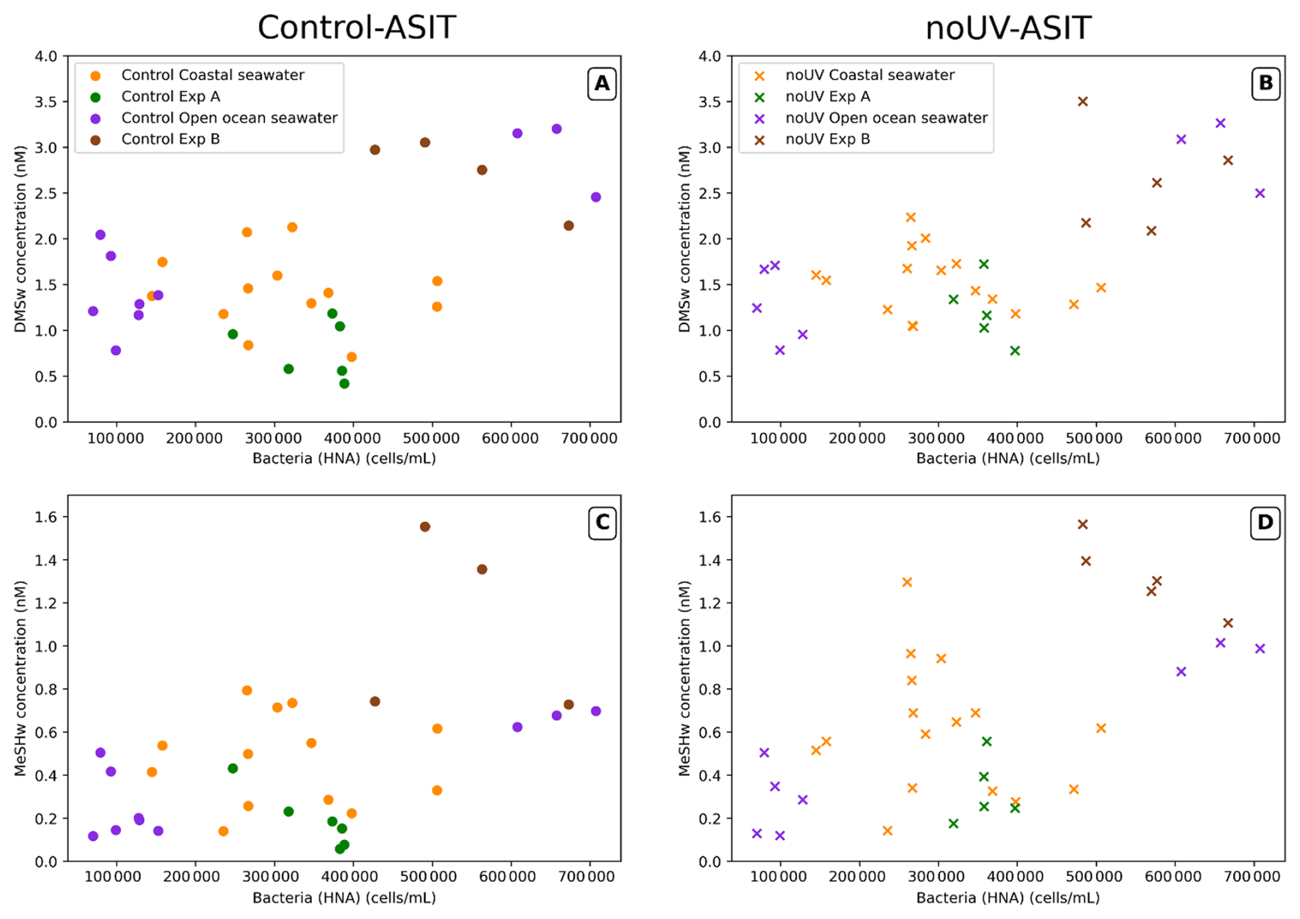
Figure 12 Scatter plots of calculated aqueous DMSw (A, B) and MeSHw (C, D) concentrations and the abundance of high-DNA bacteria. Points are coloured according to the measurement periods (see Fig. 3).

The diel profile of $F_{\mathrm{v}}/F_{\mathrm{m}}$, typically observed in the surface ocean, where diurnal exposure to high light levels (including UV) leads to some degree of stress on the photosynthetic machinery, showed differences between the Control-ASIT and the noUV-ASIT and therefore could partially explain differences in production of MeSH during the experiments. Notably, during enclosed-water experiments, a diurnal increase in HNA bacterial abundance coincided with a severe decrease in phytoplankton's photosynthetic efficiency ($F_{\mathrm{v}}/F_{\mathrm{m}}$), and both were more acute in the presence of UV. It can be speculated that solar radiation stress in phytoplankton cells results in the release of organic compounds, including DMSP, that would have fostered bacterial growth as reflected in the increase of (active) HNA bacteria. In turns, this could have led to higher gross MeSH production by bacterial DMSP catabolism. The fact that air MeSH concentrations in the ASITs were higher during the night and higher in the noUV-ASIT points to aqueous, solar radiation dependent losses overcoming potential increases in gross MeSH production.

Furthermore, a significant positive relationship between estimated aqueous concentrations of MeSH and DMS and HNA bacterial abundances was also observed in both ASITs (Spearman ρ = 0.43 and 0.49 in Control-ASIT; ρ = 0.57 and 0.63 for noUV-ASIT, respectively for MeSH and DMS). This relationship was particularly noticeable in open ocean waters (Fig. 12). A relationship of sulfur compounds with V1 and V3 virus abundance was also observed in both ASITs during experiments but not with V2 virus (Fig. S8). As explained above, dynamic and diverse processes occurred in the ASITs experiments which differently affected the particular biogeochemical elements at play, in this case targeting the virus groups.

The positive relationship between bacteria and sulfur compounds had been previously observed during the Sea2Cloud campaign (Rocco et al., 2025b). This relationship has been documented in several studies and is explained by the ability of bacteria to cleave and demethylate-demethiolate DMSP, giving rise to DMS and MeSH, respectively (Kiene, 1996; Kilgour et al., 2022). The proportion of each compound in the production, as well as in the concentrations, depends on several factors, including (1) DMSP release by exudation or mortality of the algal producers, (2) whether or not the main algal DMSP producers harbor DMSP lyases and are therefore capable of releasing DMS as well, (3) the relative proportion of bacterial genes (and the corresponding enzymes) for cleavage and demethylation (which mostly depends on the taxonomic composition of the bacterial assemblage), and (4) the relative activity of these enzymes (which may depend on bacterial sulfur and carbon demands relative to DMSP availability) (Simó 2001; Sun et al., 2016; Hopkins et al., 2023).

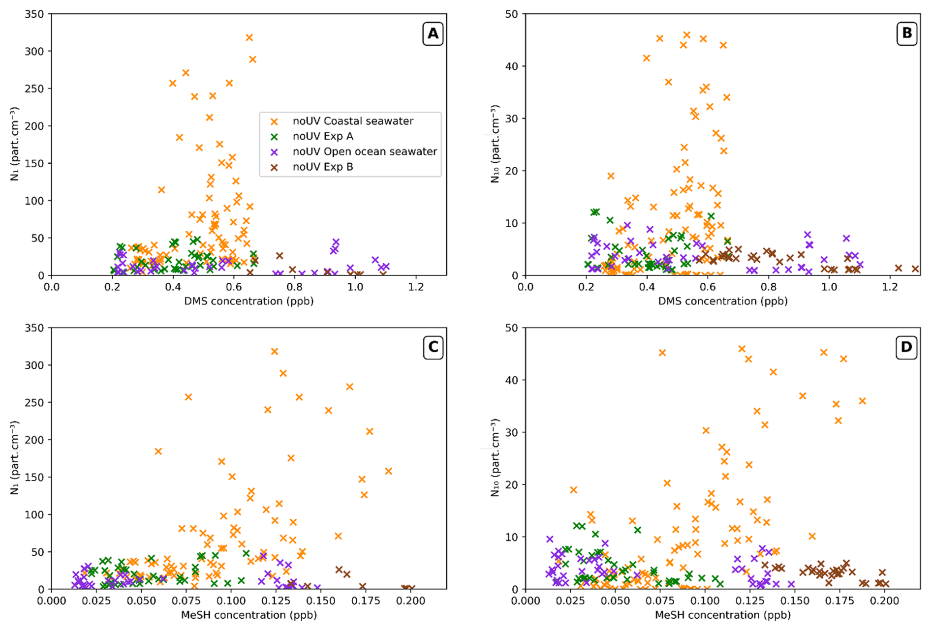
Figure 13 Scatter plots of N₁ (A, C) and N₁₀ (B, D) particle concentrations versus gaseous DMS (A, B) and MeSH (C, D) concentrations in the noUV-ASIT, with colour referring to the measurements period (as in Fig. 5).

None of the biological variables available showed a strong correlation with aqueous DMS and MeSH concentrations throughout the entire campaign when considering the continuous flow mode of our ASITs set-up, except with Chl a and bacterial abundances during the open ocean period. The non-systematic measurement of diatoms and dinoflagellates, known emitters of DMSP (Wittek et al., 2020; Sheehan and Petrou, 2020; Shaw et al., 2022), could explain this lack of correlations. During the experiments, Chl a was inversely correlated with both DMSw (Spearman ρ = −0.81) and MeSHw (ρ = −0.67), as were 1–2 and 15–20 µm SED nanophytoplankton size classes (Fig. S8A). This contrasts with the positive associations between Chl a and DMSP, the main DMS precursor, reported in Antarctic coastal and glacially influenced waters (Li et al., 2024; Petrou et al., 2026), and points to a decoupling between phytoplankton biomass and dissolved volatile sulfur compounds, whose concentrations depend on the balance between DMSP release, cleavage and subsequent removal as discussed earlier. Given the absence of DMSP measurements in the ASITs, this interpretation remains hypothetical but it must be noted that significant positive correlation was observed between DMSP and nanophytoplankton (particularly cryptophytes) in sea surface samples of the same cruise (Wohl et al., 2026).

4.3 New particle formation

The maximum particle concentrations observed during this campaign were slightly higher than those observed during the previous campaign using the same ASIT setup (Chamba et al., 2023), where N₁ particles reached concentrations of 180 particles cm⁻³, and nucleation rates were up to 0.08 $\mathrm{particles}{\mathrm{cm}}^{-\mathrm{3}}{\mathrm{s}}^{-\mathrm{1}}$. The present nucleation rates in the noUV-ASIT, reaching 0.15 $\mathrm{particles}{\mathrm{cm}}^{-\mathrm{3}}{\mathrm{s}}^{-\mathrm{1}}$, are slightly above those reported for Antarctic areas (0.05 $\mathrm{particles}{\mathrm{cm}}^{-\mathrm{3}}{\mathrm{s}}^{-\mathrm{1}}$) and below those reported for Arctic areas in the ambient open atmosphere (0.51 $\mathrm{particles}{\mathrm{cm}}^{-\mathrm{3}}{\mathrm{s}}^{-\mathrm{1}}$) (Kerminen et al., 2018).

Air MeSH concentrations showed the strongest positive correlation to N₁ and N₁₀ particle concentrations in the noUV-ASIT in continuous flow mode with coastal waters (R² = 0.56 for N₁₀; yellow in Fig. 13). This correlation degraded in the case of DMS (R² = 0.31). No significant relationship of MeSH and DMS to particle concentrations was observed in the noUV-ASIT with open ocean waters or during Experiments A and B, nor in the Control-ASIT in any observational period when particle concentrations remained low.

It is important to note that, like during the Sea2Cloud campaign (Chamba et al., 2023), no biological variable or gaseous compound showed differences between the ASITs as pronounced as the concentrations of particles, which were up to a factor of 10 higher in the noUV-ASIT. As concluded from the Sea2Cloud study, the presence of DMS and MeSH alone did not explain the formation of new particles in the enclosures. However, a significant positive correlation was found between N₁ and the 7–15 µm nanophytoplankton cell abundance during experiments (Fig. S8). This calls for further studies identifying the new particle precursors related to nanophytoplankton.

5 Conclusions

Sea–air fluxes measured inside the ASITs were always positive, i.e., degassing from seawater to air, ranging up to 8.68 $\mathrm{pmol}{\mathrm{m}}^{-\mathrm{2}}{\mathrm{s}}^{-\mathrm{1}}$ for DMS and up to 2.65 $\mathrm{pmol}{\mathrm{m}}^{-\mathrm{2}}{\mathrm{s}}^{-\mathrm{1}}$ for MeSH. DMS fluxes did not vary significantly between day and night conditions, however the $F_{\text{ASIT-MeSH}}/(F_{\text{ASIT-DMS}}+F_{\text{ASIT-MeSH}})$ ratio did have a clear maximum at night and a decrease during daytime due to diel variation in F_ASIT-MeSH. The diel pattern of the $F_{\text{ASIT-MeSH}}/(F_{\text{ASIT-DMS}}+F_{\text{ASIT-MeSH}})$ ratio could not be explained by daytime gas-phase photochemistry of MeSH compared to DMS. Estimated aqueous DMS concentrations showed maxima in the open ocean north of the Weddell Sea (2.5–3 nM) and minima in the MIZ of the Weddell Sea (1 nM) as well as in the Gerlache Strait (< 1 nM). Intermediate concentrations were estimated along the western coast of the peninsula (around 1.5–2 nM). None of the biological variables available showed a strong correlation with estimated aqueous DMS and MeSH concentrations throughout the entire campaign, although notably bacterial concentrations showed significant correlation with the aqueous concentrations during experiments and continuous flow.

A negative impact of UV-light on both DMS and MeSH sea–air fluxes was observed, with DMS fluxes being 24 % higher and MeSH fluxes 58 % higher in the noUV-ASIT compared to the Control-ASIT. Interestingly, the highest impact of filtering out UV, especially the increase of air MeSH concentrations, was seen during the night, indicating that seawater reactivity or biology had been impacted by UV during the previous diurnal period. UV light caused a slight increase in phytoplankton stress at noon and had a negative impact on the development of the smallest size nanophytoplankton (1–15 µm), especially with open-ocean waters on 7–15 µm SED nanophytoplanktons. Removal of UV-light increased the new particle formation within the ASIT headspace, with formation rates reaching 0.15 $\mathrm{particles}{\mathrm{cm}}^{-\mathrm{3}}{\mathrm{s}}^{-\mathrm{1}}$ observed with coastal waters west of the Antarctic Peninsula only in the noUV-ASIT. These nucleation rates are slightly above those reported for Antarctic areas and below those reported for Arctic areas. Newly-formed particle concentrations in the noUV-ASIT headspace were best correlated to air MeSH concentrations and to a lesser extent to DMS in run-through measurements with coastal seawaters. The presence of DMS and MeSH alone did not explain the formation of new particles in the enclosures, and no biological variable showed differences between the ASITs as pronounced as the concentrations of airborne nanoparticles, which were up to a factor of 10 higher in the enclosure with no UV light. These results call for a yet-to-identify new particle formation process that, despite being of diurnal occurrence, is enhanced by reduced UV radiation.