Assessment of vegetation water dynamics by comparing microwave remote sensing signals from satellites and field-based GNSS reflectometry

Monitoring plant water stress and biomass is limited by labor intensive measurements techniques. Observing plant water conditions more broadly is now enabled by microwave remote sensing. Specifically, satellite-based vegetation optical depth (VOD) provides daily observations of vegetation water volume at tens of kilometers. While satellite VOD has been used for many applications, VOD validations have rarely been carried out. A new method has enabled direct measurements of in-situ VOD, from Global Navigation Satellite Systems (GNSS). However, GNSS measurements have yet to be applied to more globally dominant grasslands and shrublands. Here, we explore how satellite-based VOD from SMAP and AMSR-2 compares with field-based microwave observations from 272 GNSS-based interferometric reflectometry (GNSS-IR) sites across the Western US as a part of the Plate Boundary Observatory (PBO) H₂O network. These sensors measure a proxy for VOD, or normalized microwave reflectance index (NMRI), at a much finer scale of tens of meters. We find that satellite VOD is generally positively correlated with GNSS NMRI with correlations between 0.2 to 0.6 across sites. These correlations increase to 0.3 to 0.7 when evaluating sites in regions with more homogenous vegetation types, lower tree cover, and larger seasonal vegetation dynamics. The correlations are higher for X-band VOD, likely related to our findings that X-band VOD and NMRI are both more sensitive to seasonal vegetation variations than C-band and L-band VOD products. These findings suggest that satellite VOD is capturing field-based GNSS signals in dryland ecosystems, and therefore that these sensors are a critical resource for calibrating and validating satellite VOD at scale.

1 Introduction

Vegetation regulates the water, carbon, and energy cycles at the land surface, and thus is integral to the Earth system (Gentine et al., 2019). For example, transpiration accounts for most of land water flux to the atmosphere and vegetation also alters the surface radiative balance and lower-atmosphere aerodynamics (Good et al., 2015; Wang et al., 2014). Therefore, vegetation structure and function influences lower atmospheric processes and rainfall events through land-atmosphere interactions (Green et al., 2017; Taylor et al., 2012). Natural and cultivated plants also have societal importance in supporting food security by yielding crops and forage, as well as supporting recreation (Briske et al., 2023). If vegetation dries sufficiently, it also becomes fuel for wildfire, especially in drier locations like the Western US (Orland et al., 2025). It is therefore critical to widely monitor vegetation water stress and seasonal vegetation biomass changes.

Many satellite-based optical vegetation indices, such as normalized difference vegetation index (NDVI) and solar induced fluorescence (SIF), have been used to evaluate upper canopy biomass, phenology, and ecosystem productivity (Smith et al., 2019; Tucker, 1979). For example, a primary variable for fire risk assessment, the live fuel moisture content, is commonly derived from satellite optical measurements (Yebra et al., 2013). However, these indices are largely limited by cloud cover and are sensitive only to the top-of-canopy leaves (Zeng et al., 2022). This prevents their applicability for evaluating plant hydraulics, water stress, and full canopy biomass, which requires sensitivity to water content of the full canopy and more rapid temporal sampling (otherwise reduced by cloud cover).

A more recent advance has been the use of passive microwave retrievals of vegetation water content, via an index called vegetation optical depth (VOD) (Konings et al., 2019). VOD represents the overall attenuation of the surface microwave emissions due to the vegetation canopy. VOD has the advantage of being unaffected by clouds and of being sensitive to different canopy layers, with the sensing depth increasing from mainly leaves at high frequencies (X-band; ∼ 10 GHz) to additionally the branches and trunks across the entire canopy depth at low frequencies (L-band; 1.4 GHz). The microwave vegetation signal (via VOD) was initially considered a noise source as a part of retrievals of satellite soil moisture. However, with its value in providing internal vegetation water information, VOD is now more commonly retrieved along with soil moisture across NASA's Soil Moisture Active Passive (SMAP) mission, JAXA's Advanced Microwave Scanning Radiometer (AMSR) missions, and the European Space Agency's Soil Moisture and Ocean Salinity (SMOS) mission (Konings et al., 2017; Wigneron et al., 2017; Zotta et al., 2024). As a result, the ecosystem sciences community has rapidly embraced the use of VOD over the last decade across applications, including (but not limited to) wildfire fuel load, crop yield estimation, tree mortality, aboveground biomass and carbon storage, plant water stress, and plant hydraulic traits (Anderegg et al., 2020; Brandt et al., 2018; Chaparro et al., 2018; Feldman et al., 2021c; Felton et al., 2024; Konings and Gentine, 2017; Liu et al., 2021; Tian et al., 2018). Since passive microwave retrievals have a coarse spatial resolution (∼ 30 km), such applications are implemented at regional to global scales.

However, satellite-based VOD datasets, and the related vegetation water content variable, have not been widely validated. This stands in contrast to satellite-based soil moisture for which public agencies implemented soil moisture core calibration and validation sites and field campaigns (for example, the SMAP mission and its SMAPVEX campaigns) (Chan et al., 2016; Colliander et al., 2017). In part, these field-based validation efforts were explicitly built into the mission requirements to achieve required levels of performance of soil moisture. VOD is largely not considered a part of these mission level requirements. Moreover, VOD faces substantial validation challenges compared to most other variables. First, VOD is a microwave metric that depends on both dry biomass and relative water content (Momen et al., 2017), and thus presents a challenge for measuring both of these properties in-situ requiring labor intensive and/or expensive techniques (Feldman, 2024). Additionally, passive microwave radiometers' low measurement resolution (30 km) presents the need to represent heterogeneity at the pixel scale. Therefore, a sufficient in-situ VOD validation configuration would require a substantial investment in widespread water potential measurements and dry biomass measurements across a 30 km scale, many of which may need to be measured manually and/or at a large cost.

Despite these limitations, some site-level validation efforts have been carried out to link in-situ measured VOD with canopy properties, especially using tower-mounted radiometers (Holtzman et al., 2021; Jackson and Schmugge, 1991). In these cases, tower-based radiometers are often mounted in a downward-looking configuration, with a caveat that they require partitioning of soil moisture and VOD similarly to the satellite scale. In some cases, the soil signal can be removed by covering the soil with a perfect reflector or isolating it within the VOD retrieval by directly measuring soil moisture in-situ (Meyer et al., 2018). Nevertheless, both wheat field and forested sites show promise that radiometer VOD is detecting both leaf water potential dynamics and seasonal scale changes in biomass (Holtzman et al., 2021; Meyer et al., 2018). Additionally, observing system simulation experiments (OSSEs) have been conducted to evaluate algorithmic noise sources in VOD, at least pinpointing that newer VOD retrieval algorithms, especially those that regularize VOD, are reducing VOD error variance (Crow and Feldman, 2025; Dong et al., 2018; Feldman et al., 2021a). Co-use of plant hydraulic models with VOD has also been used as a feasible method to interpret the satellite VOD signal, especially the influence of dew on VOD (Feldman et al., 2021c; Xu et al., 2021; Yao et al., 2024). However, these validation efforts remain limited and have not kept pace with the ecosystem science community's use of VOD. These field experiments need to evolve to a point at which VOD retrieval algorithms can be calibrated. Specifically, validation information is necessary to inform how to reduce VOD errors in joint retrievals with soil moisture as well as understand the influences of the mean and time dynamics of scattering albedo, first order scattering, and surface roughness effects (Baur et al., 2019, 2021; Kurum et al., 2011).

An emerging, lower cost, and less labor-intensive technique that has been implemented at the field scale relies on global navigation satellite system (GNSS) sensors. An increasingly popular configuration for VOD validation is GNSS-transmissometry (GNSS-T) approach, which positions a GNSS receiver above and below the canopy and estimates VOD as the signal difference (Humphrey and Frankenberg, 2023; Kesselring et al., 2025; Kurum et al., 2022). These configurations are typically deployed in forests with the below canopy GNSS receiver positioned above the ground to partially avoid interference from microwave soil reflectance, thus requiring the observed vegetation to be taller in stature. These sensors have been used in a dry forest in southern California, USA (Humphrey and Frankenberg, 2023), temperate forest in Missouri, USA (Yao et al., 2024), high elevation cold forest in Colorado, USA (Burns et al., 2025), among other ongoing installations. These sites have continued to establish the relationship of VOD with relative water content, leaf water potential, transpiration, and biomass. A similar GNSS-T configuration has included mobile vehicles deployed under the canopy to track differences in biomass across transects, showing the relation of GNSS-based attenuation to lidar-based vegetation height (Ghosh et al., 2024, 2025).

However, these GNSS-T configurations may be less useful for evaluating non-forested biomes with shorter statured vegetation, which encompass more than half of Earth's land surfaces. Tall enough vegetation, such as trees and some shrubs and crops, is required to sufficiently cover the receiver's hemisphere for upward-looking GNSS-T sensors (Zribi et al., 2017). Instead, GNSS configurations that take advantage of reflections from the surface can more closely measure vegetation water content of shorter statured vegetation (Larson and Small, 2014). Specifically, GNSS interferometric reflectometry (GNSS-IR) at site scales uses a fixed sensor that measures the phase difference between the direct and surface-reflected signal (Larson, 2016). These methods can use a pseudorange multipath method or signal to noise ratio interference pattern to evaluate these reflected signals (Chen et al., 2016; Larson and Small, 2014). In the case of the pseudorange multipath method – which is the method we focus on here – the phase difference between the direct microwave signal received from satellite and the weaker, indirect microwave signal reflected from the surface provide an integrated metric sensitive to both soil moisture and vegetation water content. The normalized microwave reflection index (NMRI) metric is then commonly used to partition the vegetation water content signal by controlling for surface roughness and topographical variations (Small et al., 2014). This GNSS-IR NMRI approach therefore enables evaluation of water content of shorter statured vegetation (Larson and Small, 2014), which theoretically satellite VOD should be more suited to observe than dense forests where multiple scattering often violates VOD retrieval assumptions (Chaparro et al., 2022). Note that the general idea is similar to GNSS-reflectometry being used by NASA's CYGNSS mission that uses satellites to receive the reflected signals (Asgarimehr et al., 2024). However, space-based GNSS-R missions have less temporal coverage and larger spatial footprints than ground-based GNSS-IR, as well as a limited latitudinal range of observations (38° S–38° N in the case of CYGNSS).

Evaluation of these non-forested ecosystems is critical for understanding cropland and rangeland forage yields and water stress, herbaceous vegetation fuel loads, as well as the role of grassland biomass in the carbon cycle (Allred et al., 2022; Sala and Lauenroth, 1982). GNSS-IR instruments have a legacy of use, but mainly for applications other than vegetation monitoring (Larson, 2016), and therefore could be an asset for more widespread use in the context of satellite VOD validation and plant hydraulics studies (Devine et al., 2026). These cross-scale remote sensing studies in heterogeneous dryland systems like the western US are critical, and especially aligned with the NASA Adaptation and Response in Drylands (ARID) field campaign (Feldman et al., 2024).

Across the Western US, 1100 GNSS-IR sensors were installed to evaluate plate tectonic deformation in a network called EarthScope Plate Boundary Observatory (PBO) (Larson and Small, 2014). Previous research demonstrates that grass and shrub vegetation water content can be monitored using the NMRI metric, which controls for soil moisture, soil properties (type, roughness), and topographic influences (Larson and Small, 2014). NMRI is available at a subset of PBO sites. NMRI has been shown to directly relate to in-situ measurements of vegetation water content (Jones et al., 2014; Small et al., 2014; Zhang et al., 2017). Despite its physical difference from VOD, GNSS NMRI retrievals are likely the closest, most feasible and relatively cost-effective method (approximately 10 000 USD per sensor with newer options closer to 1000 USD) to directly capture the microwave signal from these shorter statured vegetation types across an approximately 100 m scale. NMRI has been initially determined to represent a similar signature as satellite-based VOD to some degree (Jones et al., 2014; Zotta et al., 2024), and PBO NMRI has been used along with satellite measurements to create joint VWC products (Li and Sawada, 2022; Pan et al., 2020; Zotta et al., 2026). However, a more comprehensive comparison between GNSS NMRI and satellite-based VOD is needed across timescales, vegetation types, and microwave algorithms to evaluate its usefulness as a resource for calibration and validation. This is especially important for validating SMAP and SMOS based VOD as well as for upcoming multi-frequency Copernicus Imaging Microwave Radiometer (CIMR) measurements (Kilic et al., 2018). Such evaluations also serve as a precursor for comparisons between GNSS NMRI and higher spatial resolution vegetation water content retrievals from synthetic aperture radar (SAR) (i.e., NISAR, Sentinel-1) (Hajj et al., 2019).

Here we ask: do site-level microwave measurements with GNSS-based reflectometry show potential for validating and providing insights into satellite microwave vegetation retrievals? What factors impact correlations between site and satellite vegetation microwave measurements? We provide an initial assessment of GNSS-IR sites across the Western US and investigate how GNSS NMRI and satellite VOD correlate across vegetation type, spatial heterogeneity of vegetation within the satellite footprint, microwave measurement frequency, and retrieval algorithm. We also evaluate differences across timescales including correlations at seasonal timescales, related to phenology, versus daily anomalies, and related to response to rainfall events. Given that both satellite VOD and GNSS NMRI have errors, we do not present either metric as closer to the true vegetation water content, as both of their capabilities of capturing true vegetation moisture and biomass dynamics are not yet known.

2 Methods

2.1 Datasets

Our main datasets for the analysis included GNSS-IR sites and satellite VOD products across a common April 2015 to December 2017 period when all data products are available. GNSS-IR sites are used from the PBO network, from which we used the NMRI metric that was produced as a part of the PBO H₂O initiative to translate these signals to hydrologic variables (Larson, 2016; Larson and Small, 2014). While newer GNSS instruments measure all constellations, the PBO instruments (Trimble NetRs receiver, TRM29659.00 antenna with SCIT radome) only measure GPS constellation signals. Our study domain is the western US in the coterminous US where most PBO instruments are located (removing Alaska sites). There are ultimately 272 sites that have an NMRI time series in our study period and spatial domain. NMRI is a normalized metric computed via:

$$\begin{array}{}\text{(1)}& \mathrm{NMRI}=-{\displaystyle \frac{({\mathrm{MP}}_{\mathrm{1}}\mathrm{rms}-\max ({\mathrm{MP}}_{\mathrm{1}}\mathrm{rms}\left)\right)}{\max \left({\mathrm{MP}}_{\mathrm{1}}\mathrm{rms}\right)}}\end{array}$$

where MP₁rms represents vegetation attenuation as well as structure and surface roughness from the downward reflected microwave signal incoming from GPS sensors at the 1.575 GHz frequency (L-band) (Larson and Small, 2014). MP₁ stands for multipath pseudorange and rms refers to the root mean square of this signal. The maximum refers to the average of the largest 5 % of values in the time series, which represents the lowest vegetation and highest bare soil coverage conditions experienced at the site (Larson and Small 2014). Such a normalization is expected to remove most surface roughness impacts on the signal, leaving NMRI more sensitive to vegetation water content variations. NMRI uses the L1 GPS signal which is transmitted at a 1.575 GHz, which is close to SMAP's 1.41 GHz frequency. A lower MP₁rms value relative to the maximum value indicates more vegetation extinction from water content presence. NMRI values during rainy days, based on North American Land Data Assimilation System (NLDAS) data, were removed to reduce some soil moisture and interception influences on the time series.

We evaluated satellite passive microwave VOD products across L-band (1.4 GHz), C-band (6.7 GHz), and X-band (10.7 GHz), and across two different types of retrieval algorithms. Namely, we used the SMAP-based L-band VOD product from the multi-temporal dual channel algorithm (MT-DCA) at a 9 km equal area scalable Earth 2 (EASE-2) grid scale (Feldman et al., 2021d; Konings et al., 2016). This MT-DCA algorithm simultaneously retrieves soil moisture and VOD, while using a regularization approach which stabilizes the retrieval and reduces algorithm-based retrieval errors (Ebtehaj and Bras, 2019; Gao et al., 2020; Konings et al., 2015). For comparison, we also used AMSR-2 VOD retrievals at C-band and X-band from the same MT-DCA algorithm, which uses SMAP soil moisture as an input (Baur et al., 2019). These retrievals are available at 36 km resolution on the EASE2 grid. Finally, we obtained AMSR-2 VOD retrievals at C-band and X-band from the land parameter retrieval model (LPRM) algorithm and regridded them to 9 km (de Jeu, 2013; Owe et al., 2008). The LPRM algorithm uses a more traditional approach of simultaneously retrieving soil moisture and VOD without a regularization process. We additionally upscaled the 9 km products to 36 km to test the impact of the grid scale on the results, specifically through linearly averaging the 16 pixels (at 9 km grid) within the 36 km pixel. We note several additional differences between the VOD algorithms. A prominent source of differences between the VOD retrieval algorithms is how they handle land surface temperature inputs in using different sources from reanalysis (Zotta et al., 2026). Our use of AMSR-2 VOD from the MT-DCA and LPRM is sensitive to these temperature differences. Furthermore, AMSR-2 instrument measures at a 55° angle, whereas SMAP's incidence angle is 40°. While these angles are already factored into the retrieved VOD values, AMSR-2's higher incidence angle likely make the microwave retrievals relatively more vegetation-sensitive than for SMAP. Finally, we use VOD from SMAP's 06:00 a.m. local measurement time and AMSR-2 VOD from its 01:30 a.m. local measurement times which these time differences are not anticipated to create substantial divergences between VOD outputs from overnight rehydration. In fact, the use of these nighttime/morning overpasses is to reduce uncertainties related to soil and canopy temperature inputs. Ultimately, the use of five different VOD products allows direct comparison across the different LPRM (traditional dual-channel approach) and MT-DCA (regularization approach) algorithms as well as across SMAP and AMSR-2 satellite instruments with different measurement frequencies (L, C, and X band).

We also used several auxiliary datasets. As an additional point of comparison with GNSS NMRI, we used satellite soil moisture from the SMAP MT-DCA retrievals (Feldman et al., 2021d). This product was used instead of the official SMAP L3 product because of known coupling of soil moisture errors with vegetation in the SMAP L3 product (Crow and Feldman, 2025; Dong et al., 2018). Therefore, the SMAP MT-DCA algorithm soil moisture is less likely to have a built-in, erroneous influence of VOD that might inflate relationships between soil moisture and VOD. We additionally used 30 m resolution land cover data derived from Landsat during 2020 (Potapov et al., 2022). Vegetation type classifications from this dataset were divided into short statured vegetation, dense short statured vegetation, cropland, and forest based on this data product's designations. The classifications are based on the Global Land Analysis and Discovery (GLAD) product definitions (Hansen et al., 2022). Short statured vegetation is shorter than 3 m, and forested areas are taller than 3 m. The dense short statured vegetation has an additional criterion of greater than 75 % vegetation cover. Cropland land use is determined from phenology metrics as well as machine learning training on high resolution imagery. The majority of sites are placed in short (32 %) and dense short statured (50 %) areas. Two percent or less of sites are in forest, desert, and crop categories. We emphasize that GNSS-IR sensors were not installed within closed canopy forests. Pixels classified as forest sites may have one of the following scenarios: the vegetation might still be of relatively short-to-medium stature (but > 3 m), the canopy is not closed where several isolated trees may be present nearby the sensor, and/or while there is dense vegetation, the pixel might have been incorrectly classified as forest (since land cover products have associated error). Finally, we used MODIS 16 d 500 m NDVI to classify growing season timing and as an additional point of comparison in our seasonality analysis (see below) (Small et al., 2018).

2.2 Correlation Analysis

We computed the daily-scale Pearson's correlation between GNSS NMRI and VOD from each of the five VOD products and computed the percentage of sites with a positive, statistically significant (p < 0.05) correlation. NMRI is reported daily while the VOD values are typically available approximately at least every three days. We therefore only used the data pairs on the days when both NMRI and VOD are available. We only evaluated the correlation between VOD and NMRI because these metrics are inherently different; it is not possible to compute meaningful root mean squared errors or absolute biases. The GNSS NMRI correlation with satellite-based SMAP soil moisture was also computed. We subtracted the NMRI correlation with soil moisture from the NMRI correlation with each of the VOD products as a test of whether the microwave vegetation signal (within NMRI) is partitioned from the soil moisture signal. Correlations are shown in boxplots throughout the study with median, interquartile range, and whiskers representing the furthest datapoint within 1.5 times the interquartile range from the 25th and 75th percentiles. Outliers are excluded and not shown in our visualizations. These correlations were also binned based on vegetation types and the satellite pixel's spatial heterogeneity. To account for vegetation types, we used both the 30 m scale vegetation type that the NMRI site is in as well as the dominant vegetation type (mode) of the satellite pixel that the GNSS site is contained within. To consider the satellite pixel scale spatial vegetation heterogeneity, we evaluated two different metrics. First, we computed the Shannon entropy of the percent coverage of each of the four land cover types via:

$$\begin{array}{}\text{(2)}& H\left(x\right)=-{\sum }_{x}p\left(x\right){\log }_{\mathrm{10}}\left(p\left(x\right)\right)\end{array}$$

where p(x) is the distribution of four values of percent coverage of the vegetation types, where x is percent coverage of a given vegetation type. The percent coverage of each land cover within a pixel is the amount of a 9 km satellite pixel occupied by 30 m resolution land cover types. In this case, the coverage does not necessarily reflect the placement of the GNSS sensor (i.e., a 9 km pixel with high percentage of forest does not mean the GNSS sensor was placed in a forest). Smaller values of H(x) represent a scenario of mostly one land cover type, or more homogenous land cover, whereas higher values indicate higher heterogeneity with a spread of multiple land cover types within the satellite pixel. The second metric we evaluated is the percentage of the land cover within the satellite pixel that the GNSS sensor exists within, which we designated the site vegetation type pervasiveness. For example, if the GNSS sensor is located within an ecosystem dominated by short statured vegetation (based on the 30 m resolution land cover data), the value for that site is the percent coverage of the short statured vegetation across the 9 km pixel. Higher values of this site vegetation type pervasiveness indicate that the site is within the dominant land cover type seen by the satellite. We binned the correlations based on these two metrics to assess their dependence on land cover heterogeneity.

2.3 Seasonal and Daily Anomaly Timescale Analysis

The correlations were additionally evaluated at different timescales of daily-scale anomalies from the seasonal cycle (to capture co-variation of high frequency variability) and across the seasonal cycles only (lower frequency variability). To separate these two timescales, we first computed the mean seasonal cycle by averaging together days from different years into mean climatology (for example, the value of the 110th day of year is the mean of the values of the 110th day of year across 2015, 2016, and 2017). See Fig. 1 for a representative site example with dense short statured vegetation with full time series at the same site in Figs. S1 and S2 in the Supplement. We only averaged together years 2015 to 2017 to remain with a common time period across the datasets, though acknowledging a lower sample size to create the average seasonal cycle. To partly mitigate this lower sample size, the mean climatology was also then smoothed with a 30 d moving average window (Fig. 1). This time series was considered the seasonal cycle with sub-monthly variability removed. To compute the daily-scale anomalies, we subtracted this seasonal average from the original time series to isolate sub-monthly variability. This analysis was carried out for NMRI and each of the satellite VOD products (Fig. 1). Thereafter, we computed the NMRI correlation with each of the VOD products at each of these two timescales. As an additional assessment of the relative degree of seasonality compared to the daily-scale frequency variations of each vegetation microwave dataset, we computed the ratio of the standard deviation of the daily-scale anomalies to the seasonal amplitude of the seasonal cycle. The seasonal amplitude was computed as the 95th percentile minus 5th percentile of the seasonal cycle.

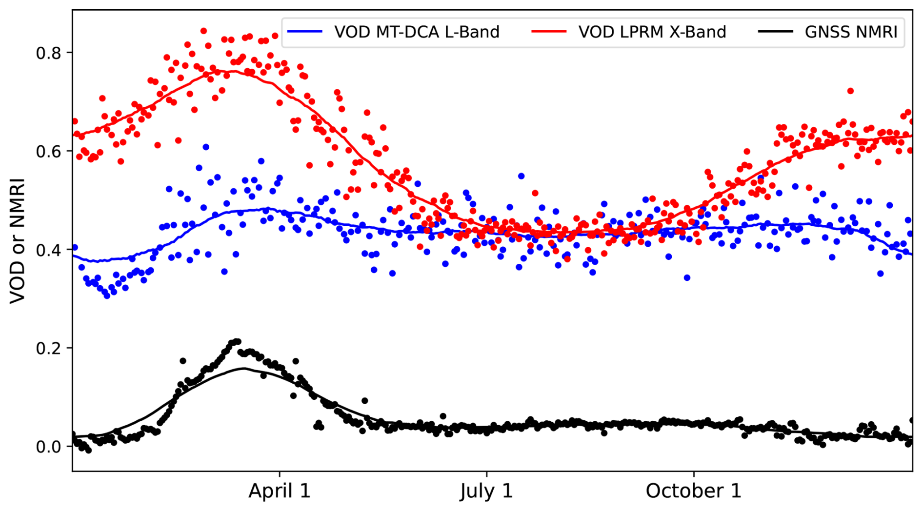
Figure 1 Example representative site (p294 PBO site) at 36.12° N and 120.44° W, which has dense short statured vegetation in California, showing time series of L-band and X-band VOD as well as of GNSS-IR NMRI. The dot symbols are averaged values over the three years of analysis (each day is averaged between 2015–2017). The solid lines are an average climatology built based on smoothing the averaged time series (dot symbols) with a moving window. Seasonal timing analyses are based on the averaged smoothed climatologies. Full time series for this site and correlation plots are shown in Figs. S1 and S2.

Next, we gave context to these correlations by evaluating more physically interpretable features of the seasonal timescales and the daily timescales. To further interpret the seasonal timescales, we compared the peak growing season timing of NMRI and satellite VOD products using two different seasonal timing metrics. The first metric used is the Julian day of the year of the peak of the smoothed seasonal cycle. The day of year peak of NMRI at each site and the satellite VOD were subtracted to compare their timing. We also used a second metric less sensitive to the peak of the seasonal cycle: the timing of the maximum positive cross correlation between NMRI and each satellite VOD product. The 16 d NDVI time series was also evaluated as a reference.

To further interpret the daily-scale anomalies, we evaluated the response of NMRI and VOD to growing season rainfall pulse events, which are expected to be detectable in dryland regions like those in the Western US (Feldman et al., 2021b). SMAP satellite soil moisture was used to identify rainfall events as an initial soil moisture increase (from previous overpass to the largest soil moisture peak before the drydown is initiated) followed by soil moisture drying over at least three consecutive SMAP overpasses (approximately 5–8 d). These surface soil moisture drydowns capture the wetting and drying associated with individual rainfall events, as demonstrated in previous studies (Akbar et al., 2018; McColl et al., 2017). Only above average soil moisture pulses were considered, which were estimated as the events where the initial increase of soil moisture is greater than the median of all events. Additionally, only soil moisture pulses during the growing season were considered in order to remove periods of no vegetation response (Collins et al., 2014). The timing of the growing season was approximated as the 180 d window around the peak NDVI determined in the above seasonality analysis. Our analysis does not appear sensitive to this definition. To normalize the VOD and NMRI responses across different sites and pulse events, the incremental rates of change per day were computed as:

$$\begin{array}{}\text{(3)}& \begin{array}{rl}& \text{NMRI Rate of Change}\\ & ={\displaystyle \frac{{\mathrm{NMRI}}_t-{\mathrm{NMRI}}_{\mathrm{tprevious}}}{t-t_{\mathrm{previous}}}}{\displaystyle \frac{\mathrm{1}}{{\mathrm{NMRI}}_{\mathrm{tprevious}}}}\end{array}\end{array}$$

where t is the respective day after the pulse and t_previous is the day of the last available measurement. The normalization by NMRI_previous makes the quantity unitless and allows comparison of relative changes after pulses across sites and different rainfall pulses within sites. Equation (3) was analogously carried out for each VOD product. Finally, for each day after the pulse ends, the 25th, 50th, and 75th percentile rates of change were computed across all pulses and sites. As an example, a positive value on day 0 indicates that NMRI typically increases from before to after the rainfall pulse event. As a summary metric at each site, we computed the percentage of rainfall pulses for which NMRI increases on day 0 of the pulse, which indicates how frequently NMRI increases after a given rainfall pulse event. The median magnitude of these post rainfall responses was computed as well. The same metrics were computed for comparison with the satellite VOD products.

2.4 Attribution Analysis

Linear and random forest regressions were carried out to attribute spatial variations in VOD-NMRI correlations as well as differences in these correlations across the VOD products. The VOD-NMRI correlations were related to several potential controlling variables across space. This includes the two land cover heterogeneity metrics (Sect. 2.2) and vegetation type information from tree cover (percent of 30 m tree cover pixels within the satellite pixel), both of which are expected to reduce the correlations. Mean climatic information was captured via mean annual soil moisture and mean NMRI, which serves as a proxy for average vegetation moisture amount. Vegetation seasonality was evaluated with the NMRI amplitude which is computed as the difference between the 95th and 5th percentiles of the NMRI smoothed climatology time series and normalized by the NMRI mean. Finally, the daily-scale variations were evaluated via the standard deviation of the VOD and NMRI anomaly time series. We refer to these variables as attribution factors.

To evaluate differences in the correlations for different VOD measurement frequencies, we subtracted the correlations between SMAP L-band MT-DCA VOD and NMRI and AMSR-2 MT-DCA X-band VOD and NMRI. These correlation differences were then linearly regressed against each of the potential attribution factors. Statistically significant correlations (p < 0.05) suggest a given factor drives a closer relation of VOD at a given frequency to NMRI. To evaluate the effects of different VOD retrieval algorithms, this same procedure was also carried out for the difference in correlations between AMSR-2 X-band MT-DCA VOD and NMRI and AMSR-2 X-band LPRM VOD and NMRI.

To evaluate the relative impacts of these attribution variables on VOD-NMRI correlations, we carried out both multiple linear regressions and random forest machine learning regressions (RandomForestRegressor function from the Scikit-learn package in Python). Specifically, attribution factors were regressed against each of the VOD data products' respective correlations with NMRI. Variances explained of attribution factors were grouped based on land cover, land cover heterogeneity, mean climate (soil moisture), satellite VOD anomaly standard deviation (with the seasonal cycle removed), and GNSS-IR based seasonal amplitudes. Use of both techniques provides insights into confidence in estimated partial sensitivities of correlations to the attribution factors (e.g., considering linear versus non-linear relations).

Finally, for those attribution factors with significant relationships, we evaluated the increase in correlations between VOD and NMRI for only the sites with higher (> 50th percentile) or lower (< 50th percentile) values of the attribution variable (depending on which direction results in increases to the correlation). This binning is expected to capture the highest and lowest potential correlations.

3 Results and Discussion

3.1 Overall site-satellite correlation patterns

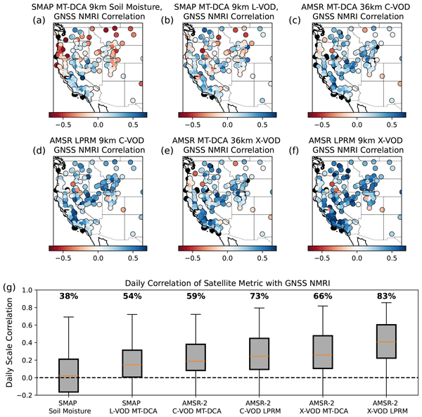
Correlations between the site-based GNSS NMRI and satellite-based VOD products are significantly (p < 0.05) positively correlated across 54 % to 83 % of the 272 considered Western US sites (depending on the VOD data product) (Fig. 2). Daily-scale correlations range from 0 to 0.6, with a median of 0.14 at L-band to 0.41 with the X-band LPRM algorithm. The X-band VOD products have higher correlations with GNSS NMRI compared to lower frequency L and C band VOD. The LPRM products also tend to have higher correlations than MT-DCA algorithms (Fig. 2). While initially appearing low, these VOD-NMRI correlations are consistently higher than when correlating NMRI with the commonly used SMAP L3 satellite soil moisture (median of 0.02) (Figs. 2, S3). This suggests NMRI and VOD are capturing microwave vegetation signals more than soil signals; if NMRI represented soil moisture signals more, the correlations between NMRI and satellite soil moisture will be higher than NMRI correlations with satellite VOD. For NMRI-VOD correlations to be higher than NMRI-soil moisture correlations, the satellite VOD signal needs to be partitioned from the soil moisture signal and the GNSS NMRI value needs to partition the microwave vegetation signal more than the soil moisture signal (acknowledging both the VOD and NMRI signal will have some relation to soil moisture).

Figure 2 Daily scale Pearson correlations between site-based GNSS NMRI and respective satellite VOD products shown spatially across (a) SMAP L-band soil moisture (9 km scale), (b) SMAP L-band MT-DCA VOD (9 km scale), (c) AMSR-2 C-band MT-DCA VOD (36 km scale), (d) AMSR-2 C-band LPRM VOD (9 km scale), (e) AMSR-2 X-band MT-DCA VOD (36 km scale), and (f) AMSR-2 X-band LPRM VOD (9 km scale). (g) The spatial distributions of the respective variable and GNSS NMRI sites are also shown in boxplots for each map, with percentages above boxplots representing the percentage of correlations that are both positive and statistically significant (p < 0.05). The SMAP soil moisture-based correlations are statistically significantly (p < 0.05) lower than that of all the VOD products based on Mann-Whitney U tests.

By contrast, analogous correlations between satellite and site level soil moisture, using the SMAP core calibration/validation sites as an example, are typically greater than 0.5 and can be as high as 0.95 (Chan et al., 2016; Colliander et al., 2017). However, there are several notable differences that should, in all cases, lead to lower correlations between VOD and GNSS NMRI. Core calibration validation sites have many distributed soil moisture sensors across the satellite pixel to capture spatial heterogeneity across the pixel (Colliander et al., 2019), whereas the GNSS comparisons here have typically only one site within the satellite pixel scale (see Sect. 3.3 for the few exceptions). Additionally, the site-level and satellite soil moisture are capturing the same metric whereas the VOD and NMRI indices are capturing vegetation attenuation in two different ways. Satellite VOD is capturing all vegetation attenuation of upwelling surface emission, while NMRI is capturing vegetation attenuation of incoming signals from satellites that observe only a fraction of the canopy per satellite overpass (Larson and Small, 2014). Finally, satellite soil moisture retrieval algorithms have been calibrated considering these site-level measurements, which will inherently improve the correlation, while VOD algorithms are largely uncalibrated to in-situ information. Therefore, lower correlations between VOD and NMRI are expected.

The results remain nearly identical when upscaling the 9 km products to 36 km to keep a consistent 36 km grid scale across all products. For example, the correlations between the LPRM 9 km correlation with NMRI are consistently similar (median correlation difference across sites of 0.004) to those when using LPRM 36 km upscaled, for both C-band and X-band. This is expected because the radiometer resolutions are 30–40 km for these sensors and the enhanced resolution from the Backus Gilbert interpolation only provides marginally finer resolution despite gridding at 9 km (Chaubell et al., 2016). We choose to remain with 9 and 36 km products because we wish to show results at the products' original gridding.

Spatial variability of correlations across the data products is apparent in Fig. 2a–f as well as in the distributions represented in Fig. 2g. Hereafter, we evaluate sources of variability in these correlations and, in particular, evaluate those that act to reduce the correlations. We investigate impacts of vegetation type, surface heterogeneity impacts due to differences in the GNSS footprint (tens of meters) and the satellite VOD footprint (tens of kilometers), measurement frequency differences, and influences of physical processes at different timescales.

3.2 Site and Pixel-Level Vegetation Type Differences

Across most conditions, correlations between GNSS NMRI and satellite VOD are higher for shorter statured vegetation and crops than for sites nearby forests or within satellite pixels with higher forest cover (Figs. 3, S4). This is especially the case for C-band and X-band VOD products. By contrast, the correlations are similar across vegetation types at L-band. While Fig. 3 presents vegetation type binned based on the 30 m land cover product, similar patterns are shown when considering the dominant land cover across the 9 km satellite pixel that contains the GNSS site (Fig. S4).

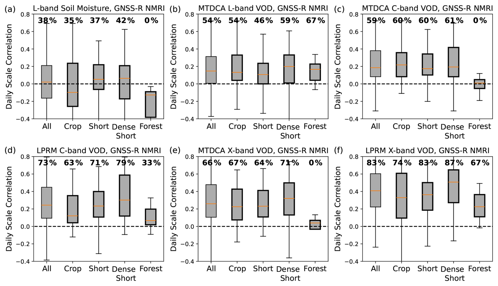
Figure 3 Daily scale correlations between GNSS NMRI and the respective satellite VOD products across different land cover types, with the same format as Fig. 2g. The land cover types here refer to that of the GNSS sites, determined from the 30 m resolution land cover type product. The same figure is shown considering the dominant land cover type across the 9 km satellite pixel that contains the GNSS sensor (Fig. S5). Percentages above boxplots represent the percentage of correlations that are both positive and statistically significant (p < 0.05).

There are several potential reasons for these patterns, especially for the lower correlations in forests at C-band and X-band. First, VOD will tend to have higher noise and variability in more forested pixels because the wavelength is often smaller than canopy constituents and thus will have more influence of multiple scattering from larger canopy structural features at the satellite pixel scale (Kurum et al., 2011). This will reduce the satellite-based VOD comparison with a field-based GNSS site. This scenario could be exacerbated where the GNSS site is located in a non-forested area, but also exists within a satellite pixel that contains a heterogeneous mixture of forests (see an example in Fig. S4). Here, C and X-band VOD will have larger errors given the smaller wavelength of less than 5 cm. Similar correlations across vegetation types for L-band VOD also support this point given that L-band VOD is less likely to be sensitive to different mixtures of vegetation types in being more capable of sensing the depth of the forest canopies in this region; the longer L-band VOD wavelength (∼ 21 cm) is less sensitive to scattering and absorption for denser canopies than for C- and X-band (Baur et al., 2019). Second, there might be smaller differences of correlations across the vegetation types as well as smaller correlations for L-band VOD overall because the VOD product is capturing more of the soil signal than C and X-band VOD products. Third, the GNSS sites with taller vegetation in their vicinity will have an influence of higher biomass and attenuation (when the signal initially traverses downward through the canopy before surface reflection) that may add more noise to the GNSS NMRI signal. However, this case is likely not a common issue given that GNSS sites were placed in mainly open areas away from collections of trees (Larson and Small, 2014).

Ultimately, the fact that correlations are highest across a range of herbaceous vegetation types is consistent with expectations of the microwaves being able to penetrate smaller canopy features (with wavelengths of 2–21 cm).

3.3 Within-satellite pixel land cover heterogeneity

We investigate how the correlations are influenced by the spatial scale mismatch of GNSS NMRI sites (∼ 100 m scales) and the satellite footprints (∼ 30 km scales) (Fig. 4). At sites with lower spatial vegetation variability, we find that correlations are higher (generally by 0.05 to 0.1) and are more commonly significant and positive. VOD correlations are highest in 9 km pixels with lower Shannon entropy of land cover types (low land cover type variability within the satellite pixel in Fig. 4). Additionally, they are higher when the GNSS site is located within that pixel's most dominant land cover type; the “site vegetation type pervasiveness” metric designation in Fig. 4 isolates the sites where the GNSS sensor is located within that pixel's dominant land cover. Taking the X-band VOD (from MT-DCA algorithm) as an example, the GNSS NMRI-VOD correlation can increase by more than 0.1 from the pixels with the highest to lowest spatial heterogeneity (Fig. 4b, c). Across most VOD datasets, this NMRI-VOD correlation significantly (p < 0.05) decreases with higher vegetation heterogeneity and increases with higher site vegetation type pervasiveness, respectively (Fig. 4b, c). Note that scatter in these plots is expected; both x-axis variables are effectively standard deviation metrics of land cover types and are correlated with a correlation variable between two noisy observations. We are quantifying whether the correlation tends to reduce when there is large spatial heterogeneity of vegetation types. These results contrast with Jones et al. (2014) which found that surface heterogeneity did not show an influence on the AMSR-E VOD and NMRI correlations. This could potentially be due to our use of a higher spatial resolution land cover data product (Landsat 30 m instead of MODIS 250 m) to estimate the spatial heterogeneity metric. We additionally find that there are correlation increases when considering only sites where the 90 m × 90 m area around the sites have the same vegetation types as that of the site, compared to those that have multiple land covers within this area (Fig. S6). However, most cases show marginal correlation differences (around 0.05) that are not necessarily statistically significant, and the vegetation heterogeneity impacting the full 9 km pixels as shown in Fig. 4a appears to more strongly influence the correlations.

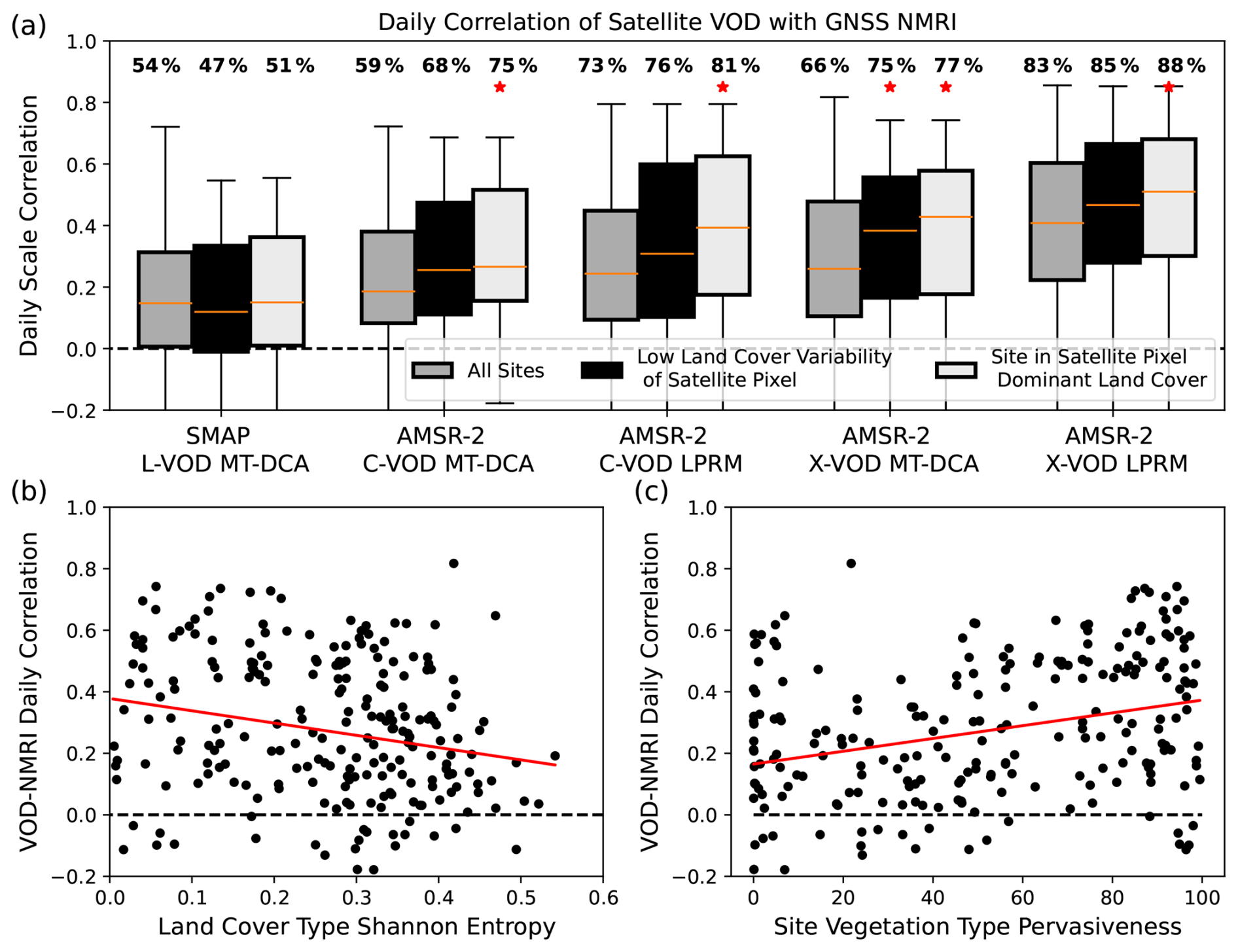
Figure 4 (a) Daily-scale correlations between GNSS NMRI site and respective satellite VOD products. Distributions of all sites are shown alongside correlation distributions in the satellite pixels with the lowest land cover variability (< 25th percentile Shannon entropy) and for GNSS sites with higher site vegetation type pervasiveness, or where the vegetation type at the GNSS site is the most dominant land cover across the 9 km satellite pixel (>75 th site vegetation type pervasiveness). Percentages above the distributions are the percentage of sites with a positive, statistically significant correlation (p < 0.05). The asterisks above the boxplot mean that the that respective distribution has correlations statistically significantly (p < 0.05) greater than the “All Sites” boxplot using Mann-Whitney U tests for differences of medians. (b) Correlations across different levels of Shannon entropy of land cover types shown in the example of GNSS NMRI correlations with X-Band VOD from AMSR-2 MT-DCA. (c) Correlations across site vegetation type pervasiveness. Higher values indicate that the GNSS site is within the satellite pixel's most dominant land cover type. Like panel (b), this considers GNSS NMRI correlations with AMSR-2 MT-DCA-based X-Band VOD. In both panels (b) and (c), the values are significantly decreasing and increasing, respectively, based on linear regressions using the raw data pairs based on both Pearson and Spearman correlations (p < 0.05; red line represents the linear regression model fit of the data). These correlations are statistically significant for all other VOD datasets except for L-Band VOD and for only site vegetation type pervasiveness for AMSR-2 LPRM X-band VOD.

We additionally evaluate the six pixels (at 9 km) that contain multiple PBO H₂O sites. We find that averaging NMRI across the sites does, on average, result in marginally higher correlations with satellite VOD than the correlations of VOD with individual GNSS-IR sites (Fig. S7). However, there are still sites within the pixel that individually have higher NMRI correlations with satellite VOD than the pixel-average NMRI. This may be because these sites represent vegetation conditions that are more representative of the satellite pixel-scale conditions than other sites are. Ultimately, it is challenging to draw generalizable conclusions since there are so few satellite pixels with more than one GNSS-IR site, only a maximum of four sites within a given pixel, and only marginal improvements on average in correlations with VOD when averaging across the sites. However, this analysis does suggest that there is a potential to increase NMRI correlations with satellite VOD by placing multiple GNSS-IR sites across a pixel to represent sub-pixel heterogeneity, as well as allow investigations into why some sites individually have lower correlations.

3.4 Measurement Frequency Differences

X-band VOD correlations with NMRI tend to be higher than correlations of NMRI with VOD at lower frequencies (Fig. 2). We evaluate the difference of L-band and X-band VOD correlations with NMRI here, where L-band VOD's correlation with GNSS NMRI is consistently lower than respective correlations of NMRI with higher frequency X-band VOD measurements (Fig. 5). This occurs both considering X-band VOD and L-band VOD retrieved using the same MT-DCA algorithm (Fig. 5a), as well as considering the X-band VOD from the LPRM algorithm (Fig. 5b). Figure 5 shows that the lower L-band VOD correlation with NMRI is relatively common, across 75 % of sites when compared to MT-DCA X-band VOD and across 86 % of sites when compared to LPRM X-band VOD. Correlations with L-band VOD being lower than those with X-band VOD of both products suggest this is also not due only to algorithmic differences. Nevertheless, the larger X-band correlations are surprising considering NMRI is based on the L-band GNSS satellite signal, and thus in theory NMRI should relate more closely to L-band VOD. Such a result is not unique to SMAP or the MT-DCA algorithm since lower correlations with NMRI were also found for a different L-band VOD product that integrates L-band measurements from SMAP as well as Soil Moisture and Ocean Salinity (SMOS) satellites (Zotta et al., 2024).

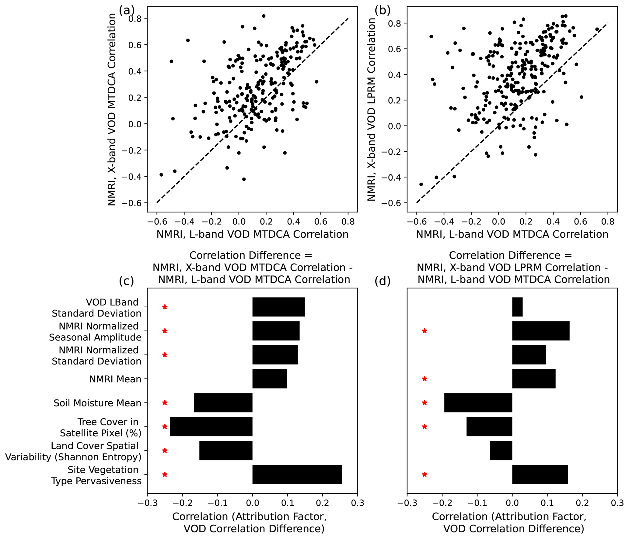
Figure 5 Comparison of correlations between L-band VOD with GNSS NMRI with the correlations of NMRI with (a) X-band VOD from the MT-DCA algorithm and (b) X-band VOD from the LPRM algorithm, where each symbol represents one site. Values above the 1–1 line indicate that the X-band VOD product has a higher correlation with NMRI than L-band VOD does for that site. (c) Relations between attribution factors and the difference of correlations between NMRI with X-band MT-DCA VOD and NMRI with L-band MT-DCA VOD (difference of y and x-axis values in panel a). (d) Same as panel (c) but difference of correlations between NMRI with X-band LPRM VOD and NMRI with L-band MT-DCA VOD (difference of y and x-axis values in panel b). Scatter plots of these relationships are shown in Fig. S8 for the X-band LPRM algorithm (d) as an example.

In the typically less densely vegetated biomes of the Western US, it is possible that X-band VOD can have an improved representation of field-based microwave vegetation signals. The annual mean X-band and L-band VOD are highly correlated (r=0.73 across the sites) with no indication of saturation at X-band, suggesting that X-band VOD is at least as suitable for observing a biomass signal similarly to the biomass signal as L-band in short-statured vegetation (Olivares-Cabello et al., 2023). Furthermore, several factors appear to be associated with higher X-band VOD correlations with GNSS sites relative to those of L-band, including lower spatial heterogeneity, lower tree cover, drier soils, higher mean NMRI, and larger NMRI seasonal amplitude (Fig. 5c, d). Notably, X-band VOD has closer relationships with NMRI variations in drier environments with less tree cover, suggesting that X-band VOD is potentially better representing the typically less dense vegetation in these mostly dry environments (Fig. 5c, d). In principle, these shorter statured vegetation types may cause similar attenuation between X-band and L-band signals. X-band VOD has lower correlations with NMRI in forested locations, especially relative to L-band, which supports this idea. Two potential error sources reduce VOD and NMRI correlations in forested pixels. Importantly, more forest cover in a pixel will result in more multiple scattering and more error retrieving VOD (Kurum et al., 2011), and especially at higher frequencies. Furthermore, NMRI is potentially reduced in its comparison to VOD when the sites are nearby forested areas because the NMRI signal becomes more dependent on the pathways of incoming GNSS signals that might initially travel through taller vegetation structures before being reflected from the ground. While only 2 % of sites are classified as forest, 11 % have adjacent pixels (at 30 m scale) that are classified as forest. This means that for these sites the type of vegetation within the NMRI hotspot likely changes over time depending on the location of the available GPS satellites within the receiver's hemisphere, and thus different vegetation types (including trees instead of only grasses or shrubs) are likely sampled over time (Devine et al., 2026; Jones et al., 2014; Small et al., 2014). This is in contrast to VOD observing all directions of upwelling emission across canopy geometries. Finally, larger seasonal amplitudes of NMRI may also relate to larger X-band VOD relations with NMRI, suggesting that X-VOD more closely resembles the seasonal cycle of NMRI and/or that NMRI is highly sensitive to the seasonality of the vegetation structure than observed with L-band VOD.

The fact that L-band VOD correlations are similar across vegetation types and land cover heterogeneity is consistent with the expectation of being less prone to signal saturation in denser canopies than higher frequencies; the L-band VOD signal is less influenced by variations in vegetation types across the pixel. By contrast, X-band VOD increases its correlations with GNSS NMRI under lower spatial heterogeneity of vegetation types within a pixel (Fig. 5); the X-band signal across the pixel scale may be relatively more influenced by vegetation scattering of smaller leaves and branches and thus responds more to the sub-pixel vegetation heterogeneity than L-band VOD.

Another potential reason for lower L-band VOD correlations with NMRI is that the L-band emission across the satellite pixel is likely relatively more sensitive to soil moisture than C-band and X-band emission, especially in these less vegetated environments and under drier soils (Fig. 5). Indeed, under dry soil conditions, the L-band emission originates from deeper soil layers which should increase the relative sensitivity of the L-band emission to soil moisture over the vegetation signal (Moghaddam et al., 2000). Analogously, site level experiments with L-band versus even longer-wavelength P-band show that P-band emission loses sensitivity to the vegetation signal and gains sensitivity to soil moisture (Shen et al., 2024). Longer wavelengths could thus create more uncertainty retrieving VOD at these sites that have less dense vegetation.

3.5 Timescale Differences: Seasonality Versus Daily Scale Anomalies

To provide additional context and attribution for our results, we also analyzed differences in GNSS NMRI-satellite VOD correlations for seasonal cycles (with daily scale anomalies removed) and daily-scale anomalies (with seasonal cycles removed) (Fig. 6a). Across all VOD products, VOD and NMRI have higher seasonal cycle correlations compared to daily-scale anomaly correlations. Such an increase of associations between seasonal cycles compared to other timescales is expected across many geophysical variables and can be due to a common climatic forcing (i.e. incoming solar radiation) rather than causal relations between the variables (Tuttle and Salvucci, 2017). Additionally, the process of isolating the seasonal cycle removes high frequency noise sources, which inherently increases seasonal-scale correlations. By contrast, correlations for daily-scale anomalies will be inherently lower because common seasonal scale forcing in the time series is removed and high frequency noise sources remain. As another source of higher seasonal-scale correlations, NMRI has a substantial seasonal amplitude relative to its mean (Fig. 6b) and relative to its high frequency variations (Fig. 6c). The satellite-based VOD products by contrast have relatively larger high frequency variations.

Figure 6 (a) Daily scale correlations decomposed into correlations between GNSS NMRI and satellite VOD for their daily scale anomalies only (high frequency variability) and seasonal cycles only (low frequency variability). (b) Ratio of the respective metric's high frequency variability and seasonal amplitude to annual scale mean. (c) Ratio of the respective metric's high frequency variability to its seasonal amplitude. Lower values, especially below 1, indicate the seasonal variations are relatively larger than the metric's high frequency variability.

As an initial insight from this partitioning, an increased correlation for NMRI with X-band VOD (Fig. 2) is likely related to X-band VOD's ability to track more features of the NMRI seasonal cycle relative to C-band and L-band VOD (Fig. 6). A larger seasonal amplitude increases the X-band VOD correlation with NMRI relative to the correlation with L-band VOD (Fig. 6). One potential reason is that, like X-band VOD, GNSS NMRI may have a relatively higher sensitivity to the vegetation structure and biomass signals, as evidenced in X-band VOD's and NMRI's relatively low daily scale variability compared to their seasonal amplitudes (Fig. 6b). Such strong relative relation of X-band VOD to biomass has been estimated previously (Zhang et al., 2019).

Ultimately, the partitioning of these timescales allows attribution of physically based sources of differences in the correlations, namely seasonal timing and rainfall pulse response of VOD and NMRI. We explore these points respectively in Sect. 3.5.1 and 3.5.2.

3.5.1 Seasonal Timing and Phenology

The seasonal peak timing of VOD from all products typically occurs within 30 d before NMRI peaks (Fig. 7). VOD therefore compares more closely to the seasonal timing of GNSS NMRI than soil moisture which peaks 50–100 d before NMRI. Note that soil moisture is expected to peak before vegetation-based seasonalities where vegetation has a delayed seasonal response to soil moisture (Tian et al., 2018), especially in water-limited locations in the western US. Additionally, the seasonal timing of NMRI is typically closer to VOD than NDVI, with similar lags between these variables captured previously (Evans et al., 2014; Wang et al., 2020). These findings suggest that NMRI and VOD are detecting similar temporal vegetation features including their biomass and relative water content, rather than only moisture sources or only upper canopy functioning (greenness, photosynthetic functioning). The seasonal peak of VOD is nonetheless earlier than that of NMRI, which is consistent with a seasonality analysis by Jones et al. (2014). While that study suggested that the earlier seasonal peak of VOD was due to differences in capturing scattering from smaller leaf and branch elements (due to their use of X-band instead of L-band VOD), we instead find a similar timing of seasonality of L-band VOD.

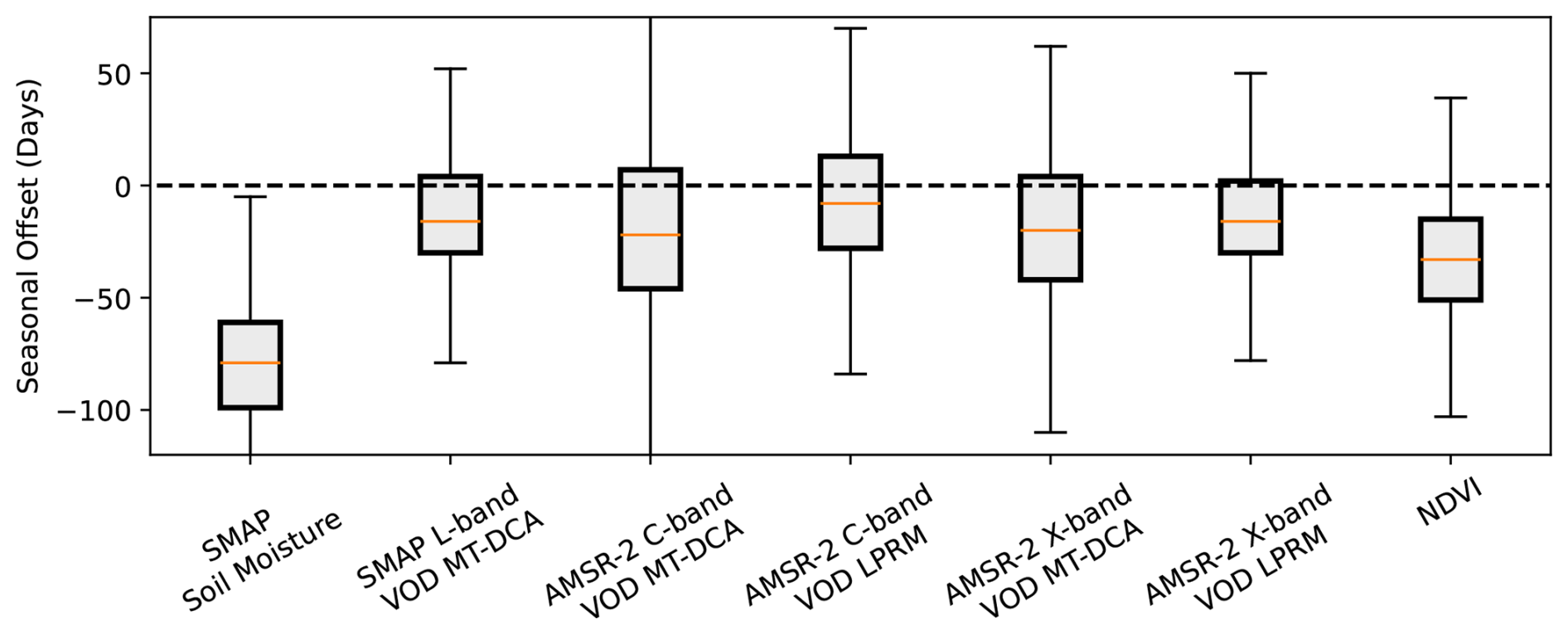
Figure 7 Difference of NMRI seasonal peak timing with respective satellite-based metric across the available GNSS sites. The peak timing refers to the difference of NMRI seasonal cycle peak with that of the respective metric. Negative values mean that the respective product peaks before the NMRI seasonal peak. All VOD-based products have statistically significantly smaller seasonal offsets than NDVI and soil moisture, based on Mann-Whitney U tests (p < 0.05). A similar plot is shown using cross correlations in Fig. S9.

Some differences in seasonality of VOD and NMRI and their overall low correlations in some cases (Fig. 2) suggest that fundamental differences in what VOD and NMRI physically represent, rather than differences in measurement frequencies alone, substantially influence each of their dynamics. GNSS-IR evaluates individual path lengths of L-band signals through a canopy, with a downward pass through the canopy, surface reflection, and an upward pass through the canopy. This is physically different from the upwelling emission measured by passive microwave radiometers (from which VOD is derived) across a 30 km area. GNSS-IR signals are rotationally polarized while SMAP and AMSR-2 passive microwave radiometers record linearly polarized signals. Finally, GNSS-IR represents smaller spatial scales that may not be representative of the larger radiometer pixels. Nevertheless, after removing effects of surface roughness, NMRI is like VOD in that both primarily represent attenuation of microwaves passing through a canopy (Jones et al., 2014).

Seasonal timing offsets between VOD and NMRI likely cause negative correlations in some cases, especially when offsets are larger (Figs. 2, 7). This is especially the case for negative correlations for soil moisture. There does not appear to be a consistent pattern with what causes negative correlations in a given VOD product. This is supported by the fact that Fig. 5 shows larger correlations between X-band VOD with NMRI (with the highest absolute value correlations amongst VOD products) typically co-occur with larger correlations between L-band VOD with NMRI (with the lowest absolute value correlations amongst VOD products) (Fig. 5); cases of negative correlations are outliers.

3.5.2 Daily Scale Rainfall Pulse Response

At daily timescales, microwave vegetation metrics are known to be sensitive to rehydration and growth following rainfall events (Feldman et al., 2021c; Anoop et al., 2024). These can occur immediately and/or continuously in the several days following the rainfall pulse. During the growing season, the GNSS NMRI signal typically exhibits an initial increase immediately following the rainfall event (on day 0, which represents pre-pulse to during-pulse conditions), likely representing rehydration of leaves and xylem (Fig. 8a) (Feldman et al., 2021c). A GNSS-T study suggests interception could also play a role in these daily-scale dynamics (Schellenberg et al., 2024), though days with direct rainfall were removed from NMRI time series and thus will play no role except when NLDAS rainfall data are imperfect. This is followed by several days of decreases likely due to plant drying during the ensuing dry spell. However, only the MT-DCA based VOD products (especially C and X-band, Fig. 8b, c, e) resemble this pattern with an initial increase followed by decreases. In fact, the C-band MT-DCA VOD product shows multi-day initial increases, while the other products rapidly switch to VOD decreases during drying one day after the rain event. The LPRM based C- and X-band VOD products likely resemble noise at this timescale with nearly equal increases and decreases in VOD following the rain event with broad scatter. This difference in algorithms is expected because the MT-DCA uses a regularization method that reduces VOD noise especially at the sub-weekly scale (Ebtehaj and Bras, 2019; Feldman et al., 2021a). By contrast, the LPRM's simultaneous soil moisture-VOD retrieval approach is more susceptible to noise at these timescales (Dong et al., 2018), which appears to manifest as random fluctuations at sub-weekly timescales. Additionally, AMSR-2-based VOD is particularly susceptible to radio frequency interference in the US (Zotta et al., 2024).

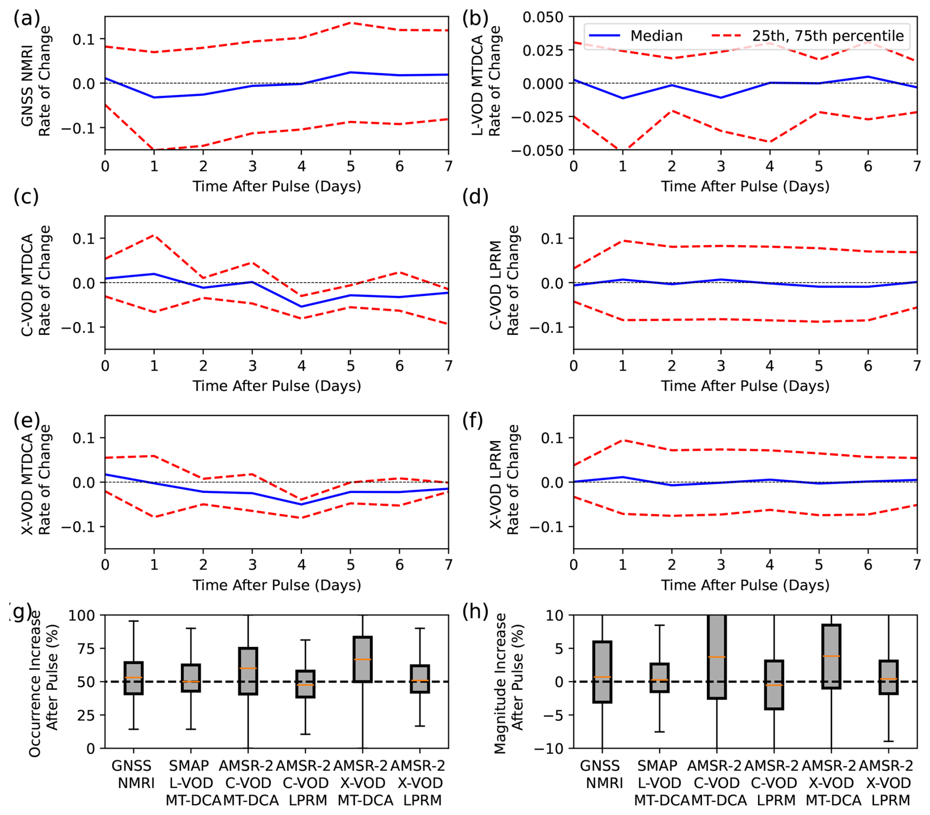
Figure 8 Responses of NMRI and VOD following rainfall events in the growing season. (a–f) Median rate of change responses following rainfall events in the growing season, as computed with Eq. (3), where positive values indicate increases relative to the previous day. Results are shown for the median across sites as well as the 25th and 75th percentile. An increase on day zero, for example, indicates typical increases from before to the end of the rainfall. The dashed line is at values of zero for reference. Note the reduced y-axis limits in panel f given smaller relative MT-DCA L-band VOD variations. (g) Percentage of occurrences of increases following pulses on day 0 of the dry spell (immediately following the rainfall event). (h) The median magnitude of response of the respective products in g. Positive values indicate more common increases of the metric immediately following rainfall events.

We further quantify how often VOD and NMRI increase the day immediately following the rainfall pulse, to test if rehydration (and potentially interception) is detected (Fig. 8g). We find that the MT-DCA algorithms all have median values typically above 50 % (L-band at 53 %, C-band at 59 %, X-band at 65 %), while the LPRM algorithms exhibit values at or below 50 % (C-band at 48 %, X-band at 50 %). The NMRI median is 53 %, which compares more closely to the L-band MT-DCA algorithm VOD product. Such a comparison is expected given some noise reduction due to regularization, which should act to increase this value whereas noise decreases it (Feldman et al., 2021a).

However, while some of the VOD products analyzed appear to capture rainfall pulse responses, there is notably wide response variability (Fig. 8g, h). Since the daily scale rainfall pulse-drydown response is a component of the daily-scale anomalies, this range of responses to rainfall pulses and general mismatch between VOD and NMRI across the products partly explains why the daily-scale anomaly correlations between VOD and NMRI are low (Fig. 6a). These results may suggest that GNSS NMRI is relatively more suitable for evaluating seasonal changes in vegetation canopy structure and moisture changes rather than daily scale changes in relative water content levels, especially with VOD and NMRI showing more similar seasonal cycles than daily scale anomalies (Figs. 6, 7). Additionally, NMRI may be capturing less daily scale variability of vegetation relative water content with its daily-scale variability relatively more subdued than satellite VOD (Fig. 6c). Some initial GNSS-transmissometry based results tend to support GNSS signals' lack of representation of internal water content compared to seasonal biomass variations (Burns et al., 2025). Potentially, the vegetation water content relationship with NMRI found at some PBO sites is more related to the seasonal rather than daily scale variations (Jones et al., 2014; Small et al., 2014).

3.6 Algorithmic Differences

X-band LPRM VOD correlations with NMRI are consistently higher than X-band MT-DCA VOD across 82 % of sites (Fig. 9), which suggests that elements of the LPRM better represent NMRI in these ecosystems. This is considering that we upscaled the LPRM product to 36 km (originally at 9 km) to be consistent with that of the MT-DCA algorithm. The LPRM algorithm does have relatively lower correlations with NMRI compared to the MT-DCA at sites where VOD high frequency variability is higher (Fig. S10). This reduction is related to VOD errors when simultaneously retrieving soil moisture and VOD, which is partly mitigated within the MT-DCA (Feldman et al., 2021a), and manifests in less representation of the pulse responses seen in the NMRI signal (Fig. 8e, f). However, vegetation seasonality is dominating NMRI and VOD correlations (Figs. 6, 7), and therefore shows increased relationships with NMRI where the NMRI seasonal amplitude is larger (Fig. S11). The LPRM algorithm also appears to better represent NMRI in more heterogeneous and more forested sites (Fig. S10).

Figure 9 Comparison between the correlation of GNSS NMRI with X-band VOD from the MT-DCA algorithm and the correlation of GNSS NMRI with X-band VOD from the LPRM algorithm. Values below the 1–1 line indicate higher correlations of the LPRM algorithm with NMRI. Both VOD products are on a common 36 km grid, removing effects of differences in resolution.

Ultimately, the differences in correlation demonstrate that there are algorithmic-based differences in VOD detectable in this analysis; there may be a means to increase VOD correlations with GNSS NMRI solely by altering the retrieval algorithms. Therefore, GNSS-IR sites show value for calibrating VOD-based algorithms with initial efforts underway (Zotta et al., 2026). This is despite potentially large representativeness errors that may initially appear to limit GNSS-IR's utility for calibration and validation. As an example, shifts in the mean and variations of scattering albedo, land surface temperature, and surface roughness can substantially change the VOD time series (Baur et al., 2019; Feldman et al., 2018; Zhao et al., 2024), which suggests that these correlations can change substantially if altering these parameters. Thus, GNSS-IR sites may be used to calibrate these parameters and other VOD retrieval algorithm uncertainties.

3.7 Potential Correlations

Based on the former analysis, we estimate the impact of several potential factors on the correlations between satellite VOD and NMRI. These include spatial heterogeneity (the two metrics in Fig. 4), land cover (percent grass and tree cover), mean climate (mean soil moisture), high frequency VOD variations, and NMRI degree of seasonality. The microwave vegetation signal seasonality appears to be the most important factor describing correlations, for both regression approaches and especially pronounced for the multiple linear regression approach (Fig. 10). Namely, these correlations tend to increase when the microwave vegetation signal contains a greater seasonal amplitude. However, other factors can increase the site-satellite correlations as well including drier moisture conditions and less tree cover (Fig. 10). The reported relative importances should be interpreted with caution considering the regressions often have total variances explained of less than 0.4, owing in part to regressing on uncertain correlation values. Additionally, the linear relationships appeared to be a best fit, whereas random forest regression methods had lower variances explained overall, suggesting that these relationships are best described as linear (Fig. S13). Nevertheless, statistically significant (p < 0.05) correlations do exist between the site-satellite correlations and these individual factors suggesting that these factors all may play a direct role in altering connections between site and satellite vegetation microwave signals (Figs. 10b, S11, S12).

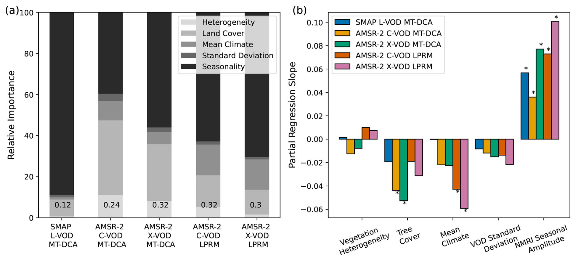
Figure 10 (a) Relative feature importance of vegetation heterogeneity, land cover type (tree, grass cover), mean climate (soil moisture), standard deviation (satellite VOD), and seasonality (GNSS NMRI) for explaining the NMRI-VOD correlations using multiple linear regressions. Total variance explained is shown in text for each bar plot, which is used to normalize the partial variances explained (relative importance). Linear regressions are shown because random forest regressions tended to have lower variances explained (Fig. S13); this is likely due to linearity of the interactions and thus simpler linear models fitting the data. (b) The partial regression coefficients between individual factors and the respective NMRI-VOD correlations. Positive values indicate increases in that variable increase the correlations between NMRI and satellite VOD. Asterisks are noted above boxplots for statistically significant partial regression coefficients (p < 0.05). Examples of individual linear regressions between explanatory factors and correlations between VOD and NMRI are shown in Figs. S11 and S12.

Overall, GNSS NMRI correlations with satellite VOD are generally higher in sites where there is low spatial vegetation heterogeneity, low forest cover, drier soil moisture, and larger seasonal NMRI amplitude (Figs. 10b, S11, S12). For the “highest potential” relations, we specifically bin sites that have greater than 50th percentile NMRI amplitude, less than 50th percentile soil moisture and tree cover across the western US, and only sites located in the dominant land cover type for that pixel (Fig. 11). 14 % of sites meet these conditions and have correlations that are statistically significantly higher (p < 0.05 from Kruskal-Wallis tests) than considering all sites together. These higher potential correlations are typically between 0.4 to 0.6. For the “lower potential” correlations, sites were selected with the opposite conditions to the “higher potential” correlations, which account for 8 % of the sites. These sites have correlations that are statistically significantly lower (p < 0.05 from Kruskal-Wallis tests) than both all sites and higher potential correlation sites. In nearly all cases, these correlations are below 0.2.

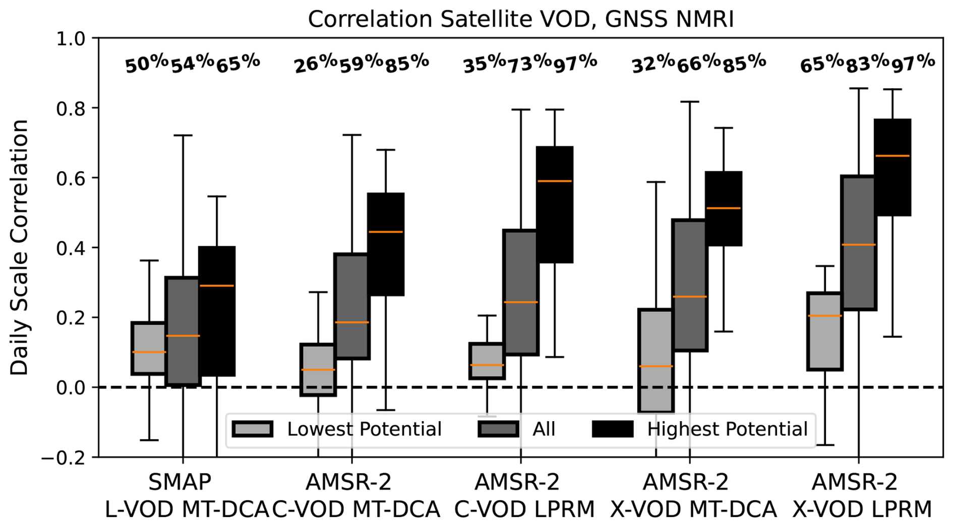
Figure 11 The spatial distributions of the respective variable and GNSS NMRI sites, with percentages above boxplots representing the percentage of correlations that are both positive and statistically significant (p < 0.05). “Highest potential” are sites binned based on all the following criteria of low land cover heterogeneity in the pixel, lower soil moisture, less tree cover, and higher seasonal amplitudes, respectively. By contrast, “lowest potential” are sites binned based on all the following criteria of high land cover heterogeneity in the pixel, higher soil moisture, more tree cover, and lower seasonal amplitudes, respectively.

First, such an analysis demonstrates that there are physically explainable conditions for higher correlations in some sites, such that placement of GNSS sites matters for broader landscape representation of vegetation conditions and for satellite VOD validation. Second, the analysis may reveal an upper bound relationship between a single GNSS-IR site and satellite VOD retrieval over that site; this relationship is otherwise still limited to values near 0.6 due partly to the spatial scale mismatch and differences in representation of VOD and NMRI. Potentially, the relationship could still increase with the use of more sensors throughout the site. These sites under these criteria may also serve as the key sites selected for algorithmic calibration of satellite VOD products, under which calibration may serve to increase this relationship.

The potential correlations increase to above 0.4 and often around 0.6 when using higher frequency C- and X-band VOD, especially from the LPRM algorithm and when sites with larger seasonal cycles are considered (Figs. 2, 11). We hypothesize that both X-band and NMRI more closely represent the seasonality of vegetation structure in these ecosystems dominated by shorter statured vegetation, compared to L-band VOD. Several sources of evidence from these potential correlation findings combined with seasonality analyses (Sect. 3.5) support this hypothesis. First, the X-band VOD correlations with NMRI are highest considering only the correlations of their seasonal cycles (Fig. 6a) and because the X-band correlations increase when the vegetation seasonal amplitude is larger (Fig. 10b). Both NMRI and X-band VOD also have relatively larger seasonal amplitudes relative to their daily-scale variations (Fig. 6b). L-band VOD, on the other hand, does not significantly increase its relationship with NMRI in sites with higher NMRI seasonal amplitudes (Fig. 10b). L-band VOD might be relatively more sensitive to short-term variations in relative water content (Fig. 6) especially with the use of the MT-DCA algorithm that uses regularization to reduce noise at shorter timescale. NMRI nevertheless appears less sensitive to these shorter-term variations (Fig. 6b), and thus higher frequency C- and X-band VOD might unexpectedly have closer representation to NMRI.

4 Conclusions

Correlations between GNSS NMRI and satellite VOD range between 0.2 and 0.6, showing some promise for GNSS NMRI to be used as a field-based method of observing water content of shorter statured vegetation canopies and a scalable means of validation of satellite VOD. However, while microwave GNSS-IR measurements and satellite VOD retrievals should observe the same vegetation canopy features (plant saturation and biomass), we find several site characteristics that tend to reduce these correlations. These include, but are not limited to, within-satellite pixel heterogeneity of land cover and wetter ecosystems with more tree cover. Therefore, these correlations tend to increase to between 0.4 and 0.6 when GNSS sensors are placed in canopies that constitute the dominant land cover within the pixel, when the satellite pixel has more homogeneous land cover, and when drier and shorter statured, non-forested canopies are evaluated.

The correlations also further increase to between 0.6 and 0.8 when using X-band VOD, especially from the LPRM algorithm, as well as when sites with larger seasonal cycles are considered. This result is unexpected given that GNSS-IR at the PBO H₂O networks are measuring signals from L-band navigation satellites, and thus L-band VOD should theoretically have a closer comparison than X-band VOD with NMRI. However, unlike GNSS-T configurations, GNSS NMRI depends in part on how microwaves pass through the canopy including a reflection from the surface, which might increase the dependence of NMRI on the vegetation canopy structure. Our analysis points to X-band VOD, like NMRI, being more sensitive to seasonality of vegetation structure than L-band, especially for these shorter statured canopies in the Western US. This is related to the fact that, like NMRI, X-band VOD has a larger seasonal amplitude compared to shorter timescale variations, which suggests more sensitivity to biomass or structure variations than to rapid plant hydraulic variations. L-band VOD, by contrast, appears to have relatively more sensitivity to shorter-term variations likely related to daily-scale changes in relative water content.

Furthermore, satellite VOD correlations with site-level NMRI might be relatively low and seasonality timing different because the metrics have fundamental differences. Beyond differences in spatial scale, this includes VOD and NMRI differences in representation (two individual paths through canopy including reflection from surface versus integrated upwelling emission), footprint (variable hotspot and incidence angle for GNSS-IR), and polarization differences (rotational versus linear polarization). The extent to which these considerations reduce VOD and NMRI relationships is currently not well known and needs to be further tested. VOD from radar might mitigate these differences in being similarly sensitive to surface microwave reflections and in having a higher spatial resolution.

Despite differences between field NMRI and satellite VOD, our results show promise that GNSS-IR sites can be used to monitor vegetation water content in spatially dominant grassland and shrubland ecosystems, whereas the increasingly implemented GNSS-T sites are mainly suitable to evaluate tall-statured ecosystems (i.e., forests). When considering the most ideal site conditions to compare the satellite VOD to NMRI, correlations increase to a range between 0.3 to 0.7, suggesting that satellite VOD is feasibly resembling a microwave vegetation signal. These VOD-NMRI correlations are higher than with satellite soil moisture, suggesting that NMRI and satellite VOD are detecting a microwave vegetation and less so a soil moisture signal. If choosing X-band only, these correlations are typically above 0.6. By extension, this means that GNSS-IR sites can be used as calibration and validation tools for satellite VOD retrievals across different products, in the cases where these sensors are in more ideal conditions (“highest potential” cases in Fig. 11). Such efforts are already underway for AMSR (Zotta et al., 2026), and thus may be useful for calibrating VOD products from SMAP and SMOS as well as upcoming NISAR and CMIR products. Operational VOD products have historically not been calibrated to in-situ vegetation information. Thus, our findings point to a potential for improved VOD data products by using these sites as VOD calibration and validation opportunities in grassland and shrubland sites. In cases where NMRI and VOD do not closely relate, these provide further opportunities to understand causes of the mismatch to provide further insight into calibration and validation efforts.

Based on our results, we recommend further investigation of joint use of microwave vegetation signals from satellite VOD and GNSS-IR sensors, including installing several instruments within a satellite pixel to properly represent sub-pixel heterogeneity and capture the satellite-scale VOD signal. These sensors should be used in conjunction with GNSS-T sensors to represent grassland, savanna, and forested regions to both evaluate their vegetation water dynamics and validate satellite VOD. We also recommend GNSS-IR based studies along with site level instruments like dendrometers and psychrometers, like those available in the PSInet database to further improve the potential to link microwave signals and plant behaviour (Pierrat et al., 2025; Restrepo-Acevedo et al., 2024). We encourage extending the analysis to comparing GNSS NMRI to higher spatial resolution synthetic aperture radar measurements like with C-band Sentinel-1 and L-band NISAR. Finally, such cross-scale studies with microwave measurements of vegetation are critical for understanding plant water stress and short-term drought adaptation and tolerance in dryland ecosystems. This study namely serves as a first step for scaling and validation activities for the NASA ARID campaign, which is focused on the domain of this study in the western US (Feldman et al., 2024).