
the Creative Commons Attribution 4.0 License.
the Creative Commons Attribution 4.0 License.
 | 17 Nov 2026
Disentangling the biotic and abiotic drivers of evapotranspiration in a degraded raised bog
Vincent E. Flemming

Nicolas Behrens
Mana Gharun
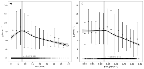
Despite covering only approximately 3 % of the Earth's land surface, peatlands are recognized as a key nature-based solution for climate change mitigation due to their substantial carbon storage and high potential for restoration. Beyond carbon sequestration, peatlands also influence the local climate through land–atmosphere energy exchange, with one of their key cooling mechanisms being the regulation of latent heat fluxes (LE). However, the interaction between abiotic (e.g., atmospheric and soil meteorological conditions) and biotic (e.g., canopy conductance (gc), gross primary productivity (GPP)) drivers on LE remains insufficiently understood, particularly in the context of drained peatlands dominated by heath and dwarf-shrub vegetation. Here, we analyzed eddy covariance measurements collected over three years between 2023 and 2025 at a drained raised bog in northwest Germany. Using high frequency CO2, H2O, energy flux, and meteorological measurements we (1) explored the daily and seasonal dynamics of LE, (2) quantified the influence of biotic and abiotic drivers on LE, and (3) determined the vegetation physiological thresholds at which gc limits LE due to an increase in atmospheric and soil dryness. To disentangle the biotic and abiotic controls of LE, we derived a continuous time series of gc by inverting the Penman-Monteith equation using 30 min LE fluxes measured with the eddy covariance method. This approach enabled us to estimate subdaily gc alongside GPP and continuous daily meteorological variables, including net radiation (Rn), air temperature (Ta), vapor pressure deficit (VPD, i.e., atmospheric dryness), groundwater table depth (WTD), and soil water content (SWC, i.e., soil dryness). Using daily mean data, detrending of mean seasonality, and removal of time lag, the variable component of the drivers was extracted and the effect size on LE was determined. Rn and GPP showed the largest effect on LE, with marked differences in their effect during the growing season versus the non-growing season. During the growing season, Rn and GPP have the largest effect on LE, while outside the growing season, WTD and VPD have the greatest impact. gc responded strongly to VPD but not to SWC. The peak of a local polynomial regression indicated the thresholds for VPD and SWC at which LE was limited by vegetation physiological responses (gc). With increase in atmospheric dryness, gc significantly limited LE above a VPD threshold of 7.6 hPa. These results help us better understand the potential impacts of environmental conditions on the evaporative cooling capacity of drained peatlands. Further research is needed to understand how occurrence of extreme climatic conditions will affect the relationships identified in this study.
- Article
(3131 KB) - Full-text XML
-
Supplement
(864 KB) - BibTeX
- EndNote


Evapotranspiration (ET) is a key component of the land water cycle as a large portion of water reaching land via precipitation (P) is removed through ET (Türk et al., 2026; Wilusz et al., 2017). ET is the transfer of water from surface (evaporation) and vegetation (transpiration) into the atmosphere, whereby liquid or solid water transforms into water vapor. The phase change of water requires energy, which is transported away as latent heat flux (LE), thereby cooling the land surface. ET and LE are thus directly related, with LE representing the energy equivalent of ET. Vegetation transpiration exchanges water vapor for CO2, making ET a key link between water cycle, energy cycle, and carbon cycle. Beyond their role in greenhouse gas uptake and carbon sequestration, the climate mitigation potential of natural ecosystems is therefore also strongly determined by their evaporative cooling capacity. Through ET-driven LE exchange, ecosystems can moderate surface temperatures, reduce heat extremes, and influence regional climate conditions, highlighting that the climate benefits of ecosystem restoration and conservation extend beyond carbon storage alone (Miralles et al., 2025).
Although peatlands cover only 3 % of global land area, they have a significant climate potential as they store around 30 % of global terrestrial soil organic carbon (Yu, 2012). In their natural state peatlands are (nearly) waterlogged ecosystems that naturally sequester and store carbon for centuries. Anthropogenic drainage for agriculture, peat cutting and forestry as well as climate change effects lead to lowered water tables, degradation of the peat and emission of the carbon as CO2. Lowered water tables reduce the water-holding capacity of the porous peat matrix, enhancing lateral water loss and altering vertical water vapor fluxes from ET (Liu et al., 2022). Vegetation change further amplifies these dynamics. In degraded peatlands, increased shrubification and dominance of woody vegetation can change transpiration rates, intensifying or lowering vertical water losses (Limpens et al., 2014). Intact peatlands possess hydrological self-regulation mechanisms that mitigate drought effects (Nijp et al., 2017). Their high water-holding capacity also makes them key regulators of hydrology, buffering both water availability (Karimi et al., 2024) and the impact of droughts (Kettridge and Waddington, 2014). However, these capacities are impaired when water levels decline.
In drained peatlands vegetation cover often shifts from mosses to heath dwarf-shrub vegetation. Vascular plants can actively regulate transpiration by opening and closing their stomata. The strategies plants have for responding to soil and air dryness vary among species (Morgan et al., 2025; Fu et al., 2022). Previous experiments in controlled environments show that transpiration in Calluna vulgaris and Molinia caerulea (vegetation that dominate our peatland of study) increases with rising vapor pressure deficit (VPD) under moist soil conditions (Gobin et al., 2015). These experiments also show that when soil is dry, transpiration of C. vulgaris initially increases with rising VPD, but decreases after a certain dryness point. Meanwhile M. caerulea shows no change in transpiration with increasing VPD under dry soil conditions (Gobin et al., 2015). These observations indicate variation in the strength of stomatal regulation among vegetation types, highlighting the complex role of vegetation in controlling transpiration. This variability can lead to contrasting effects on LE under conditions of increased warming and drying (Massmann et al., 2019).
Peatlands are considered energy-limited ecosystems (e.g., Alekseychik et al., 2017 (raised bog, boreal); Gunawardhana et al., 2021 (alpine sphag. valley bog); Sonnentag et al., 2010 (minerotrophic fen, boreal)) in which groundwater table depth (WTD) correlates with LE only when it is near or above the soil surface (Humphreys et al., 2006; Gunawardhana et al., 2021; Lafleur et al., 2005). Biotic drivers include photosynthesis at the canopy scale expressed as gross primary productivity (GPP), as well as the degree to which vascular plants regulate transpiration through stomatal opening and closure, represented by canopy conductance (gc). Through these processes, vegetation can exert a stronger control on LE than the peatland type itself (Humphreys et al., 2006).
Despite the overarching energy limitation imposed by net radiation (Rn), the roles of other drivers, such as WTD and vegetation composition, remain variable and insufficiently resolved, particularly in Central European peatlands where direct energy flux measurements are still limited. While the effects of abiotic controls (e.g., VPD) on LE are well established from a physical perspective, their interactions with biotic factors mean that the magnitude and direction of their influence on LE can vary depending on both their intensity and the prevailing vegetation composition.
Peatland conservation measures, including rewetting and vegetation management practices such as tree removal, are widely implemented across Central Europe and can directly influence LE. To identify effective conservation and restoration strategies, it is therefore essential to improve our understanding of the magnitude of these effects and the interactions among the factors controlling LE. In addition to active management, anthropogenic climate change is expected to alter peatland vegetation composition, potentially promoting shifts toward more shrubby vegetation even in the absence of direct human intervention (Heijmans et al., 2013). Such vegetation shifts are facilitated by lowered water levels and increasing temperatures (Heijmans et al., 2013) both of which are expected to intensify under future climate conditions (Shekhar et al., 2024). Understanding the interactions between biotic and abiotic controls on LE is thus critical for predicting how peatland carbon and water cycling will respond to climate change and associated shifts in environmental drivers.
We analyzed three full years of eddy covariance (EC) and micrometeorological observations from a drained bog ecosystem in northwestern Germany, aiming to (1) investigate the diurnal and seasonal dynamics of LE measured directly using the EC method, (2) quantify the relative influence of biotic (GPP, gc) and abiotic drivers (Rn, VPD, air temperature (Ta), WTD, soil water content (SWC)) on LE, and (3) identify physiological thresholds at which canopy response to environmental conditions constrains LE.
2.1 Study site
The study area is located in Amtsvenn-Hündfelder Moor (DE-Amv), North Rhine-Westphalia – Germany (52.17° N, 6.95° E, 38 m a.s.l.). This peatland covers an area of 894 ha (Europäische Union, 2021) and has been part of the Natura 2000 network since 2004, which is the world's largest contiguous network of protected areas (Directorate-General for Environment, 2000). The peatland is characterized as degraded raised bog dominated by Calluna vulgaris (L.) Hull, Erica tetralix L. and Molinia caerulea (L.) Moench. Species such as Somatochlora arctica Zetterstedt or Drosera intermedia Hayne occur here, making the ecosystem a valuable habitat (Utikal and Rückriem, 2019). Vegetation height was primarily determined by the evergreen and woody C. vulgaris (L.) Hull and averaged 30 cm. Although M. caerulea (L.) Moench and sporadic Betula spp. Exist at the site, they do not dominate the EC footprint. According to the Köppen-Geiger climate classification, DE-Amv belongs to type Cfb (warm temperate, fully humid zone with warm summers) (Kottek et al., 2006). The average annual temperature (2007–2024, Deutscher Wetterdienst (DWD), 2022) is 10.6 °C, with the coldest month being January with an average temperature of 1.1 °C and the warmest month being July with 18.3 °C. Mean annual P is 794 mm (2007–2024). The EC setup was installed in October 2022 at a height 2.8 m above the surface. DE-Amv is an official ICOS associate station.
2.2 Data
Data used in this study spans the period between 1 January 2023 and 31 December 2025. EC data, measured at a height of 2.8 m, was processed according to standard procedures, including filtering for low u* conditions and spike removal (Pastorello et al., 2020). Stevens Hydraprobe, used to measure SWC, was adjusted to organic soil. A detailed list of all available variables and measuring devices used can be found in Table 1. Missing data in meteorological variables was filled from a small meteorological ancillary tower, located 20 m from the EC tower. Additional remaining gaps were filled with XGBoost (Chen and Guestrin, 2016). Results of the gap-filling were verified on test datasets left out during model training and R2 scores exceeded 0.85 for all gaps, except for incoming longwave radiation and SWC, where R2 exceeded 0.7 for gap lengths of 40 d. Nighttime partitioning of CO2 fluxes into GPP and ecosystem respiration (Reco) was done using the REddyProc package in R (Wutzler et al., 2018). The complete list of variables measured at the site is proved in Table S1 in the Supplement.
2.3 Energy balance
To evaluate the quality of the eddy covariance measurements, we evaluated the surface energy balance for the study site. Energy balance closure was calculated using the following equation, excluding the effects of snow:
E represents the error that consists of missing parameters and measurement errors. The sign convention here is that soil heat flux (SHF), LE and H are positive upwards, and Rn is positive downwards. The energy balance was calculated using 30 min measured data without gap filling and served to verify whether the energy flux measurements were of sufficient quality to support robust analysis and interpretation.
2.4 Growing seasons identification
The growing season was identified on an annual basis using GPP. Start and end of the growing season were determined by fitting a double sigmoid function to the partitioned GPP. Start and end of the growing season were determined as the first maximum and last minimum of the third derivative of a double sigmoid function (Beck et al., 2006).
2.5 Sub-daily time series of canopy conductance
gc was modeled in a modified way according to Runkle et al. (2014), which used the inversed Penman-Monteith equation. The Penman-Monteith equation includes surface conductance as a variable instead of gc. Surface conductance is the sum of gc, soil conductance and canopy interception conductance (Nguyen et al., 2021). During the growing season, soil evaporation can be neglected; furthermore, data was filtered by P, to exclude interception evaporation, such that surface conductance ≈ gc can be assumed (Matos et al., 2025; Gharun et al., 2020; Speranskaya et al., 2024). gc was calculated by inverting the Penman-Monteith equation, for days where no P on this day and less than 2 mm P the day before occurred ( 0 mm mm}, where D is the set of days used and i is the index of the days) (Dingman, 2015):
with rH [%] as relative humidity, gat [m s−1] as atmospheric conductance, λv [MJ kg−1] is the latent heat of vaporization, γ [kPa K−1] is called the psychrometric constant, although it is not a constant (Loescher et al., 2009), ca [MJ kg−1 K−1] is the heat capacity for air, Δ [kPa K−1] is the slope of relation between saturation vapor pressure (VP) and Ta, [kPa] is the saturation VP, ρa [kg m−3] is air density and ρw=1000 kg m−3 is water density, and ca [MJ kg−1] is the heat capacity of air. These values were calculated using the following equations (Dingman, 2015):
zveg [m] stands for the vegetation height, va [m d−1] stands for wind speed, m and n are constants, and exp refers to the natural exponential function. Here, gc was calculated with 30 min data. gc was despiked to remove obviously incorrect values. To remove outliers, data points above 30 mm s−1 and below 0 mm s−1 gc were first removed; subsequently, following Rogiers et al. (2005) in an adjusted way, a rolling window of three days was applied on the data to calculate mean and standard deviation and all values larger or smaller three times the standard deviation were removed. The inverted Penman-Monteith equation does not account for missing energy storage terms (for example, the heating of the soil above the SHF sensors or the heating of the vegetation). Additional storage terms to Rn and SHF were not considered due to instrumental limitations. The 30 min gc values were restricted to the time period between 08:00 and 16:00 UTC+1 in order to exclude, on the one hand, periods of limited vegetation activity during the night and, on the other hand, periods in which the assumption of a closed energy balance in the inverted Penman-Monteith equation was frequently violated.
To retain only seasons with active vegetation, gc data was then filtered for the growing season. To determine the point at which the evaporative cooling capacity of the vegetation was limited by VPD or SWC, gc and VPD as well as gc and SWC were scattered against each other. Using a local polynomial regression analysis and nonparametric breakpoint detection, the relationship between gc and VPD, as well as gc and SWC, was determined. The regime change in gc was defined as the rightmost local maximum of the regression line. The 95 % confidence interval of the regression and the regime change in gc was determined using bootstrapping (n=1000). If gc decreases with increasing VPD or SWC, gc was limited by VPD or SWC.
2.6 Seasonal energy flux dynamics
The annual and daily variations of the energy components (Rn, SHF, H, LE) and other environmental variables (e.g., GPP, Ta) were examined visually. The composition of the turbulent energy fluxes was determined by the Bowen ratio (B). B was given as the ratio of H to LE (). To reduce the influence of outliers from negative energy fluxes, particularly during winter, the data was aggregated into three-day values. B was calculated for time periods in which Rg is above 20 W m−2.
2.7 Statistical analysis
Generalized least squares models (Aitken, 1936) with autoregressive errors (Cochrane and Orcutt, 1949) (GLSAR) of the first order (AR(1)) were used to examine the biotic and abiotic variables influencing daily average LE. GLSAR was used because eddy covariance fluxes and micrometeorological data are temporally autocorrelated, violating the independence assumption of ordinary least squares. Three models were fitted: one covering the entire period from 1 January 2023 to 31 December 2025, a second model covering the growing season, and a third model covering the non-growing season. To control for seasonal effects, in a first step ordinary least squares (OLS) models were created for all relevant predictors (Rn, GPP, VPD, Ta, WTD, and SWC), except gc, with only the months as predictors. The residuals of the OLS model were the proportions of the dependent variables that are not explained by seasonal effects, which were used as predictors for the further analysis. For all time windows (entire year, growing season, non-growing season), the data were checked for multicollinearity using the variance inflation factor (VIF), whereby all predictors had to have a VIF value of < 10 (Dormann et al., 2013). In addition, the correlation between all pairs of predictors was checked and a Pearson correlation coefficient (r) of ≤ 0.7 was required for all parameters (Dormann et al., 2013). gc was not included in the driver analysis, as it was calculated using the inverted Penman-Monteith equation, which already included Rn and is derived from LE measurements. Therefore, including gc in the driver analysis would have introduced statistical circularity.
H and soil temperature (Ts) were excluded from the models; the reason for the exclusion was a high level of multicollinearity when H was included and a strong collinearity between Ta and Ts. The detrended predictors were normalized to a mean value of 0 and a standard deviation of 1. Normalization made it possible to compare the effect sizes.
To account for temporal autocorrelation in the residuals, a GLSAR AR(1) was used. The order of AR was chosen based on a partial autocorrelation function (PACF) plot. This GLSAR AR(1) model considered the dependency between two neighboring points in time and assumed that the difference between the predicted and actual values (residuals) was not completely random, but partially influenced by the previous value, which is typical for climate data. In addition, the HC3 covariance matrix correction was used to estimate the standard errors, which ensured that the standard errors were robustly estimated even in the case of heteroscedasticity. The use of HC3 was therefore a conservative estimate of the confidence intervals and p-values.
The quality of the model was assessed using the R2 value and the Durbin-Watson statistic (DW) (Durbin and Watson, 1950, 1951, 1971). Temporal autocorrelation was assumed from a DW < 1.5 or > 2.5, whereas a value of 2 meant that no temporal autocorrelation was present.
Working with mean daily values required the time series to be complete, which in EC virtually always requires filling of gaps created during filtering steps. Assessing drivers on gap-filled data bears the danger of circularity, since data that was filled through models is inherently dependent on the predictors used. We assessed the effect of the gap-filled data on the driver analysis by fitting separate models using different thresholds of the maximum percentage of gap-filled values in each day (between 10 % and 100 %).
The GLSAR AR(1) models were compared with generalized additive mixed models (GAMMs) incorporating spline terms and the same autoregressive structure using the Akaike information criterion (AIC) (Akaike, 1974). The performance of the GLSAR AR(1) model based on year-round data was equivalent to that of the corresponding GAMM AR(1) model (ΔAIC < 1.5). In contrast, the GLSAR AR(1) models for the growing seasons and non-growing seasons were preferred over the corresponding GAMM AR(1) models based on their lower AIC values. Data transformations did not increase model performances, indicated by increased AIC values.The data processing was done with Python 3 (van Rossum and Drake, 2009), in particular the packages Numpy (Harris et al., 2020), Pandas (The pandas development team, 2025), SciPy (Virtanen et al., 2020), scikit-learn (Pedregosa et al., 2011), statsmodels (Seabold and Perktold), Ruptures (Truong et al., 2020), Matplotlib (Hunter, 2007), and Plotly (Plotly Technologies Inc., 2015) which were used to perform statistics, mathematics and data handling and to create figures.
3.1 Energy balance closure
The energy balance for the period from 1 January 2023 to 31 December 2025 was made up of a mean value of 41.2 W m−2 for LE, 22.5 W m−2 for H, 1 W m−2 for SHF, and 82.3 W m−2 for Rn. The slope of a linear regression between LE+H and Rn − SHF corresponded to 0.83 for all data (Fig. 1). For days with no P, as well as for days with more than 0 mm and up to 2 mm P, the slope of the regression was 0.82. For days with more than 2 mm P, the slope of the regression was 0.83. During the growing seasons (Sect. 3.2), the slope of the regression between LE+H and Rn − SHF corresponded to 0.83, while during the non-growing seasons it corresponded to 0.71. For daily averages of days without data gaps and for gap filled data, the energy balance closure was 0.99.
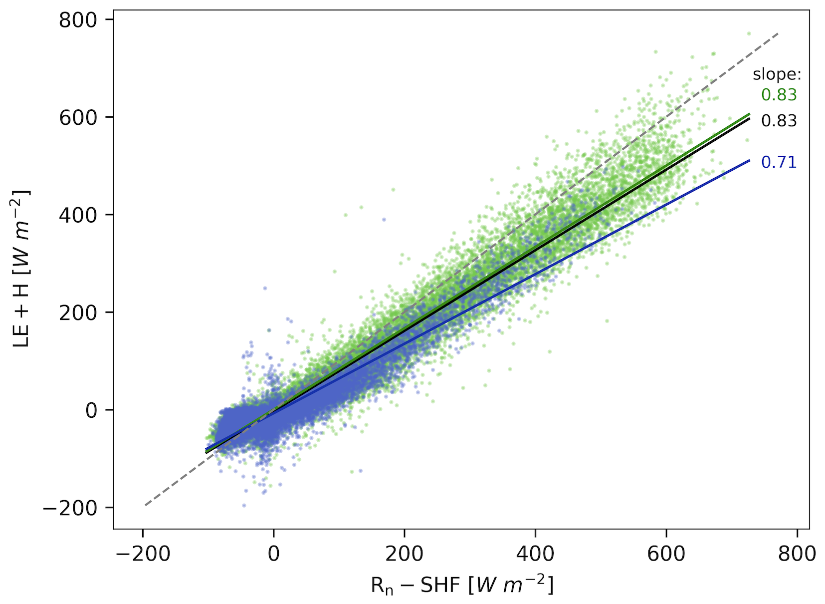
Figure 1Test of the energy balance closure in DE-Amv during the measurement period (1 January 2023 to 31 December 2025), growing season (7 April 2023 to 8 November 2023, 24 April 2024 to 24 October 2024, and 4 April 2025 to 1 November 2025), and non-growing season. The x-axis shows the difference of net radiation (Rn) and soil heat flux (SHF). The y-axis shows the mean values for latent heat flux (LE) and sensible heat flux (H). Values at 30 min resolution are scattered against each other in green for the growing season and in blue for the non-growing season. A linear regression and the slope of the straight line are shown in black for the entire measurement period, green for the growing season and blue for the non-growing season, while the gray, dashed line marks the 1:1 relationship.
3.2 Seasonal energy flux dynamics
For DE-Amv, in 2023, the growing season began on 17 April and ended on 8 November. In 2024, the growing season began on 24 March and ended on 24 October. In 2025, the growing season began on 4 April and ended on 1 November (Supplement Fig. S3).
The analysis of the monthly average daily fluctuations in the energy flux components showed clear seasonal patterns. H dominated the turbulent energy flux during most months of the first half of the year (from February to May), while LE became the dominant component later in the year (from June to September) (Fig. 2). This seasonal shift of the turbulent energy fluxes was reflected in B, which remained above 1 in the initial months before declining below 1 during June to October in 2023, May to October in 2024, and May to September in 2025 (Fig. S4).
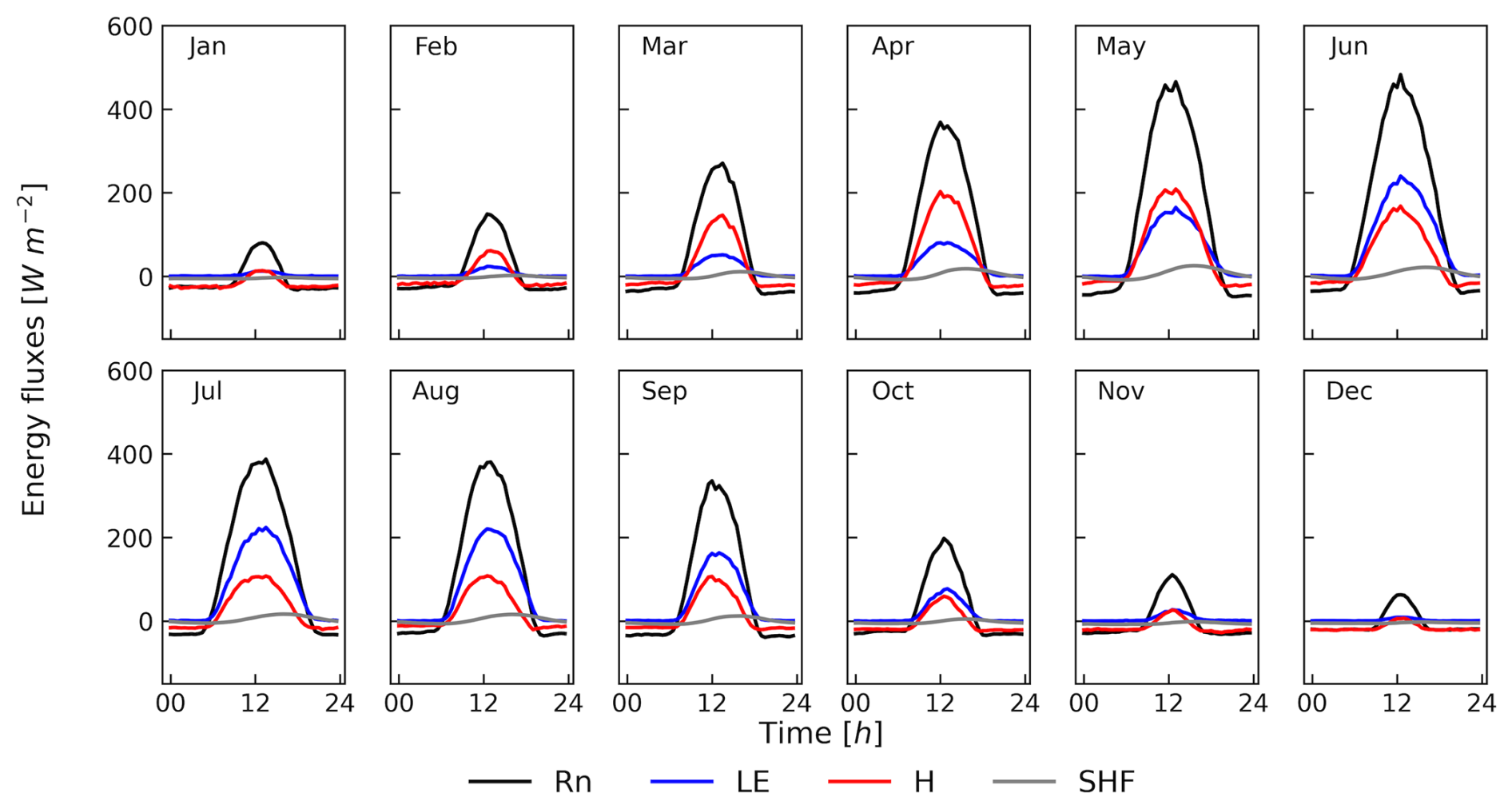
Figure 2Monthly mean diurnal radiative and turbulent energy fluxes for the measurement period (1 January 2023 to 31 December 2025): In black the net radiation (Rn), in blue the latent heat flux (LE), in red the sensible heat flux (H) and in gray the soil heat flux (SHF). The times indicate the local time of the study site.
While LE increased in the morning together with Rn, its afternoon decline was slower than that of Rn for approximately 5 h (Fig. 2). VPD and Ta also remained high during early afternoon (Fig. 3). In each month, Rn was the dominant energy component during daytime, while SHF was permanently the lowest. SHF showed a diurnal variation throughout the year, which is delayed in relation to the other energy components.
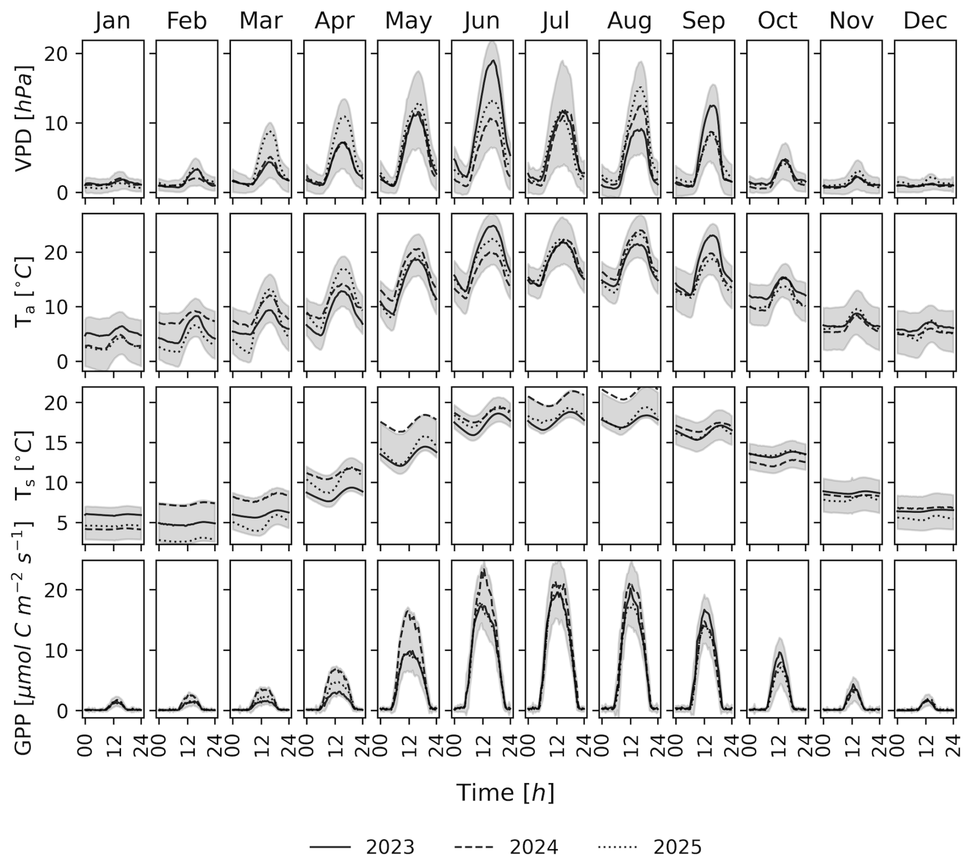
Figure 3Diurnal patterns by month. The black lines show the mean value by year (solid = 2023, dashed = 2024, dotted = 2025), while the grey area represents the standard deviation of all years (2023, 2024, and 2025) combined. VPD = vapor pressure deficit, Ta= air temperature, Ts = soil temperature, GPP = gross primary production.
During the colder months (November to February), turbulent energy fluxes were minimal, with H frequently registering negative values and LE remaining close to zero. Consequently, B also assumed negative values with considerable fluctuations. GPP exhibited a characteristic daily pattern, rising sharply in the morning, peaking before midday, and then gradually declining. This trend mirrored the course of VPD and Ta in an axisymmetric manner. Ts followed a similar pattern to SHF, with minimum values in the morning and an increase towards the evening. Nighttime values of H dropped clearly, reaching the lowest levels in winter. Conversely, LE approached zero at night, with seasonal variations in daily maxima. All four energy flux components (Rn, SHF, H, and LE) displayed steady trends over the year, with smooth transitions between seasonal extremes. The daily peaks of LE and H occurred after those of Rn but preceded SHF maxima.
Rg peaked during June for all years (Fig. 4). Ta and VPD peaked between June and August, except for 2024, where VPD had its maximum value in May. SWC was measured at multiple locations, showing consistent trends between locations, despite local heterogeneities. The driest soil conditions were observed in late June and August of 2025, whereas the wettest period occurred during the transitions of the years 2023 and 2024, and 2024 and 2025. P exhibited seasonal variability, with the lowest amount recorded in March 2025 (3 mm per month) and the highest in July 2024 (170.8 mm per month). The by far most intense rainfall event occurred at the 21 July 2024 (72.2 mm d−1). WTD fluctuated throughout the year, being closer to the surface from January to mid-May before gradually declining until October. Over the three years considered, WTD showed a declining trend.
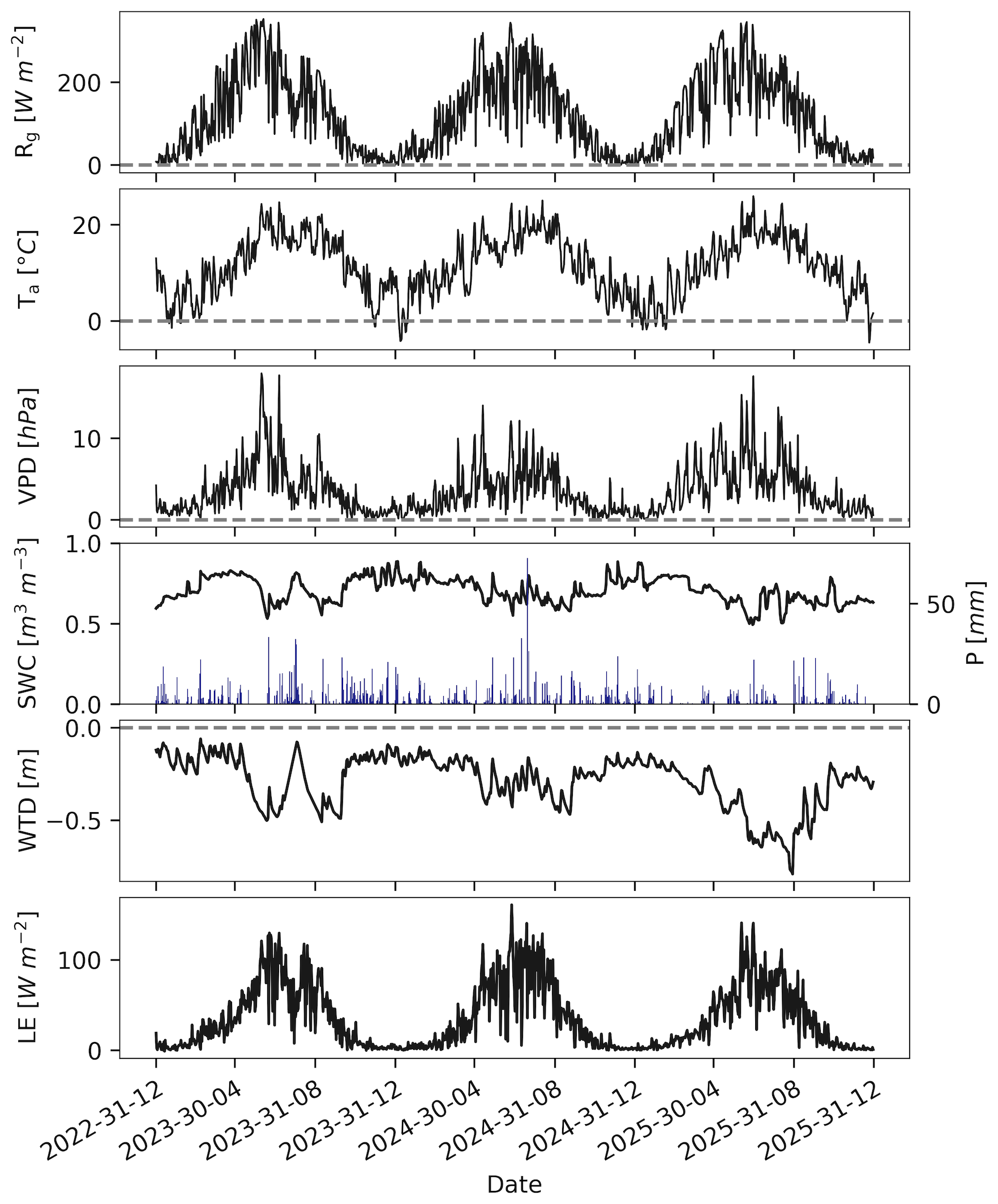
Figure 4Global radiation (Rg), air temperature (Ta), vapor pressure deficit (VPD), soil water content (SWC) at −5 cm depth, in blue the precipitation (P), water table depth (WTD) and latent heat flux (LE) for the measurement period (1 January 2023 to 31 December 2025). The data is displayed at a daily resolution.
LE reached its highest values in mid-June to beginning of July. Although general trends were evident, deviations could be observed in all measured variables; for instance, Rg showed frequent high values in early summer (mid-May to June) 2023, which aligned with local maxima in Ta and VPD, coinciding with a drier period marked by low SWC and WTD. Albedo was highest during July and August (a=0.15 for 2023, a=0.17 for 2024, and a=0.13 for 2025) and lowest during December (a=0.05 for 2023, 0.04 for 2024, and 0.06 for 2025).
Annual P reached 1007 mm yr−1 in DE-Amv in 2023, 914 mm yr−1 in 2024, and 562 mm yr−1 in 2025. 2023, average Ta reached 11.5 °C in DE-Amv. Annual average Ta was 11.6 °C in 2024 and 11 °C in 2025. Mean monthly temperature in DE-Amv was 5.3 °C in January 2023, 3.2 in January 2024, and 2.9 in January 2025 and 17.8 °C in July 2023, 18.3 °C in July 2024, and 18.4 °C in July 2025. SWC ranged from 49 % (30 June 2025) to 89 % (5 January 2024) (Fig. 4). WTD ranged from −79 cm (30 August 2025) to 0 cm (10 March 2023). Ts reached its minimum at the 20 February 2025 at 0.7 °C and its maximum 15 August 2024 at around 23 °C.
3.3 Driver analysis
The GLSAR AR(1) regression results indicated a strong model fit for the entire year and during the growing season. In all trained models VIF values were well below 10 and between the explanatory variables all R values were less than 0.7. The proportion of gap-filled data permitted within daily datapoints had little impact on the driver analysis. Minor effects were observed only when the threshold was reduced to 10 %; however, this resulted in substantial data subsampling, rendering the analysis less representative. Both the ranking and the magnitude of all drivers remained consistent across the full range of thresholds for the maximum allowable proportion of gap-filled data per day (Fig. S1).
Table 1Metrics of GLSAR AR(1) models. Data is from 1 January 2023 to 31 December 2025 and the growing season is taking place from 17 April 2023 to 8 November 2023, 24 March 2024 to 24 October 2024, 4 April 2025 to 1 November 2025. DW = Durbin-Watson. Model significance is indicated by p < 0.001.
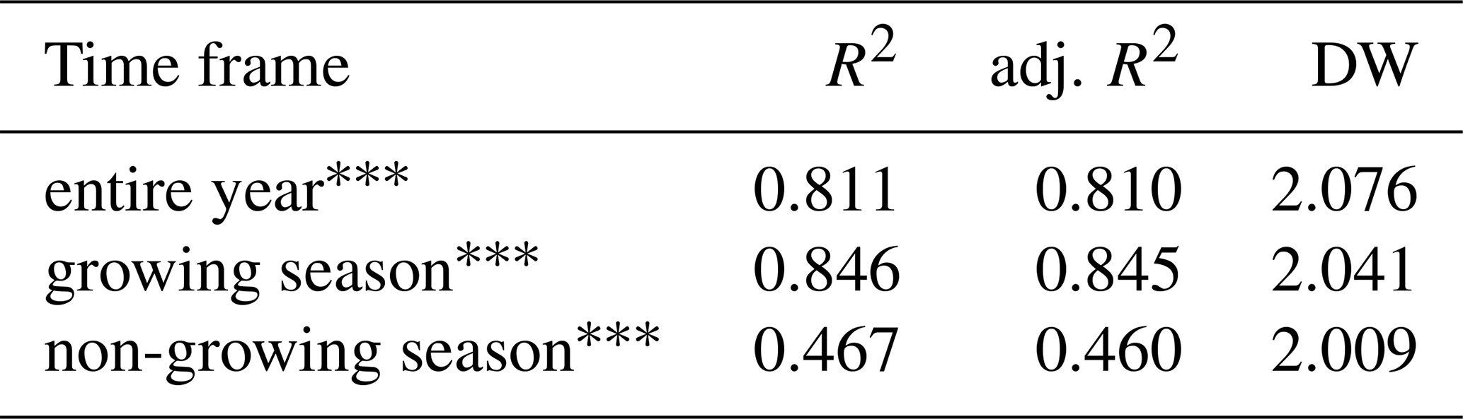
For the entire years 2023 to 2025, the model exhibited a high goodness of fit with an R2 of 0.811 and an adjusted R2 of 0.810 (Table 1). The F-statistic of 379.5 (p < 0.001) confirmed the overall significance of the model. The DW statistics of 2.076 suggested that temporal autocorrelation had been effectively corrected. During the growing seasons (17 April 2023 to 8 November 2023, 24 March 2024 to 24 October 2024, 4 April 2025 to 1 November 2025), the model fit improved further, with an R2 of 0.846 and an adjusted R2 of 0.845. The F-statistic of 410.2 (p < 0.001) further confirmed the strong explanatory power of the predictors also in the model for the growing seasons. The DW statistics of 2.041 remained close to the ideal value of 2, indicating near no autocorrelation. In contrast, the non-growing season showed a weaker model fit, with an R2 of 0.461 and an adjusted R2 of 0.460. Despite the lower explanatory power, the model remained statistically significant (F-statistic = 40.98, p < 0.001). The DW statistics of 2.009 suggested a good level of autocorrelation correction.
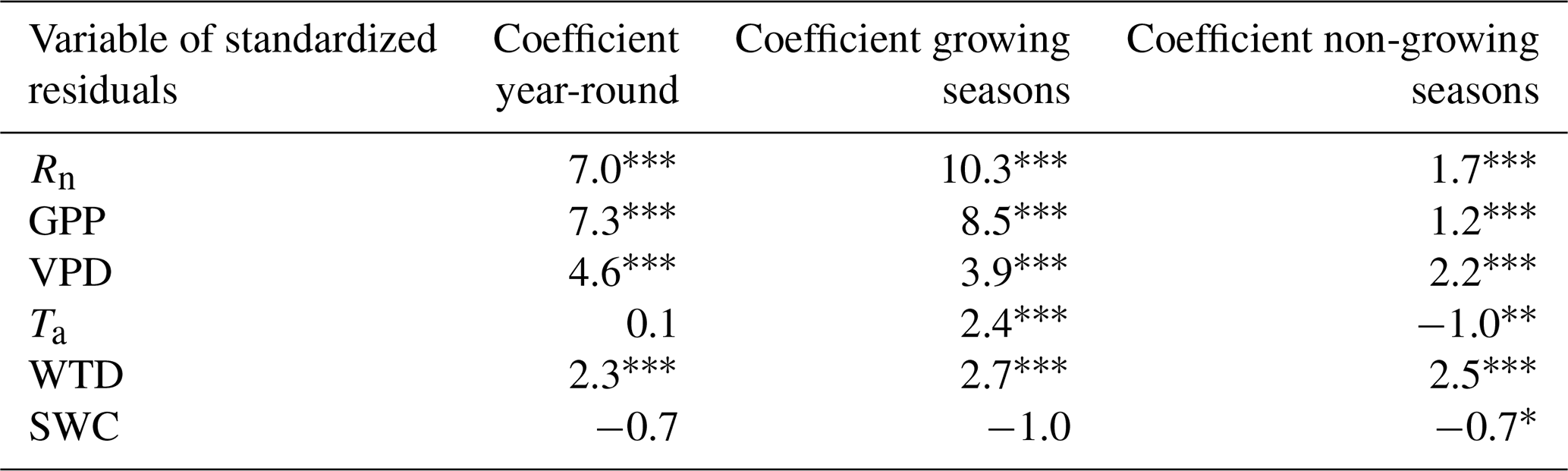
In the entire years 2023 to 2025, the standardized residuals of GPP, VPD, Rn, and WTD exhibited significant positive effects on LE, with coefficients of 7.3 for GPP, 7.0 for Rn, 4.6 for VPD, and 2.3 for WTD (p < 0.001) (Table 2). SWC showed no significant positive effect on LE, also, Ta has no significant effect on LE. During the growing seasons, all parameters considered, except SWC, showed a significant influence on LE. Rn influence on LE was notably stronger compared to the annual results and now has an effect size of 10.3. GPP also gains further weight during the growing season and with 8.5 had a larger effect size than VPD during this time. With a coefficient of 3.9 VPD remained an important predictor, while Ta has a medium positive effect on LE (2.4). During the non-growing season, WTD and VPD had by far the strongest effect, although at 2.5 for WTD and 2.2 for VPD they were weaker than in the previous two time periods. GPP also in the non-growing season had a significant effect on LE, although at 1.2 the effect size was small. Rn and Ta almost had no influence on LE. With −1 Ta's effect on LE is negative during the non-growing season. SWC revealed a slightly significant effect during the non-growing season (p=0.042), although the effect size of −0.7 is negligible.
Table 2Results of the GLSAR AR(1) models. The coefficients of the variables of standardized residuals are shown for the entire period from 2023 to 2025, the growing seasons (17 April 2023, to 8 November 2023, 24 April 2024 to 24 October 2024, and 4 April 2025, to 1 November 2025), as well as the non-growing seasons. Rn = net radiation, GPP = gross primary production, VPD = vapor pressure deficit, Ta= air temperature, WTD = water table depth, and SWC = soil water content. * p < 0.05, p < 0.01, p < 0.001.
3.4 Canopy conductance
gc reached its highest daily maximum in July and August, while the smallest daily variations with the lowest maximum values were observed in April and May (Fig. 5). The 30 min gc time series contained several outliers whose pronounced intensity obscured weaker outliers for the filter; nevertheless, a clear diurnal cycle is evident for all months, particularly from June through October. gc rose until around 11:00 UTC+1 and then declined continuously, with the peak occurring earlier in April and May and at around 12:00 UTC+1, later in June.
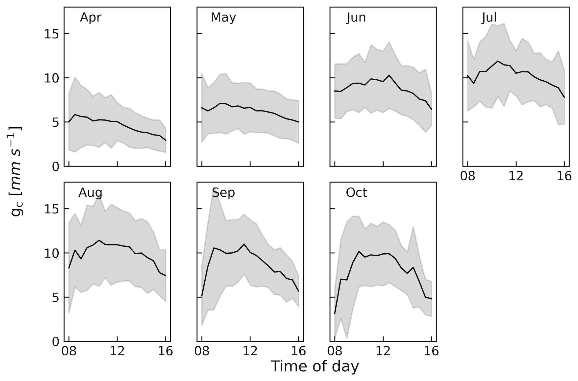
Figure 5Diurnal patterns by month. The black line shows mean canopy conductance calculated using equation 2 (gc) and the gray area shows its standard deviation. Data was restricted to the growing seasons.
The regression analysis revealed a maximum in gc at a VPD of 7.6 hPa, with a 95 % confidence interval ranging from 7.1 to 8.2 hPa (Fig. 6a). Below the threshold of 7.6 hPa VPD, gc increased with VPD, accompanied by a pronounced standard deviation. Above the threshold, gc decreased as VPD increased, and the standard deviation also decreased as VPD increased. For gc and SWC, a threshold of 62 % SWC was observed, with a 95 % confidence interval ranging from 62 % to 63 % (Fig. 6b). For values above this threshold of 62 % SWC, a decrease in gc was apparent with increasing SWC, whereas below the threshold, there was no significant correlation between gc and SWC according to the 95 % confidence interval of the regression line. The standard deviation of gc showed no trend for SWC.
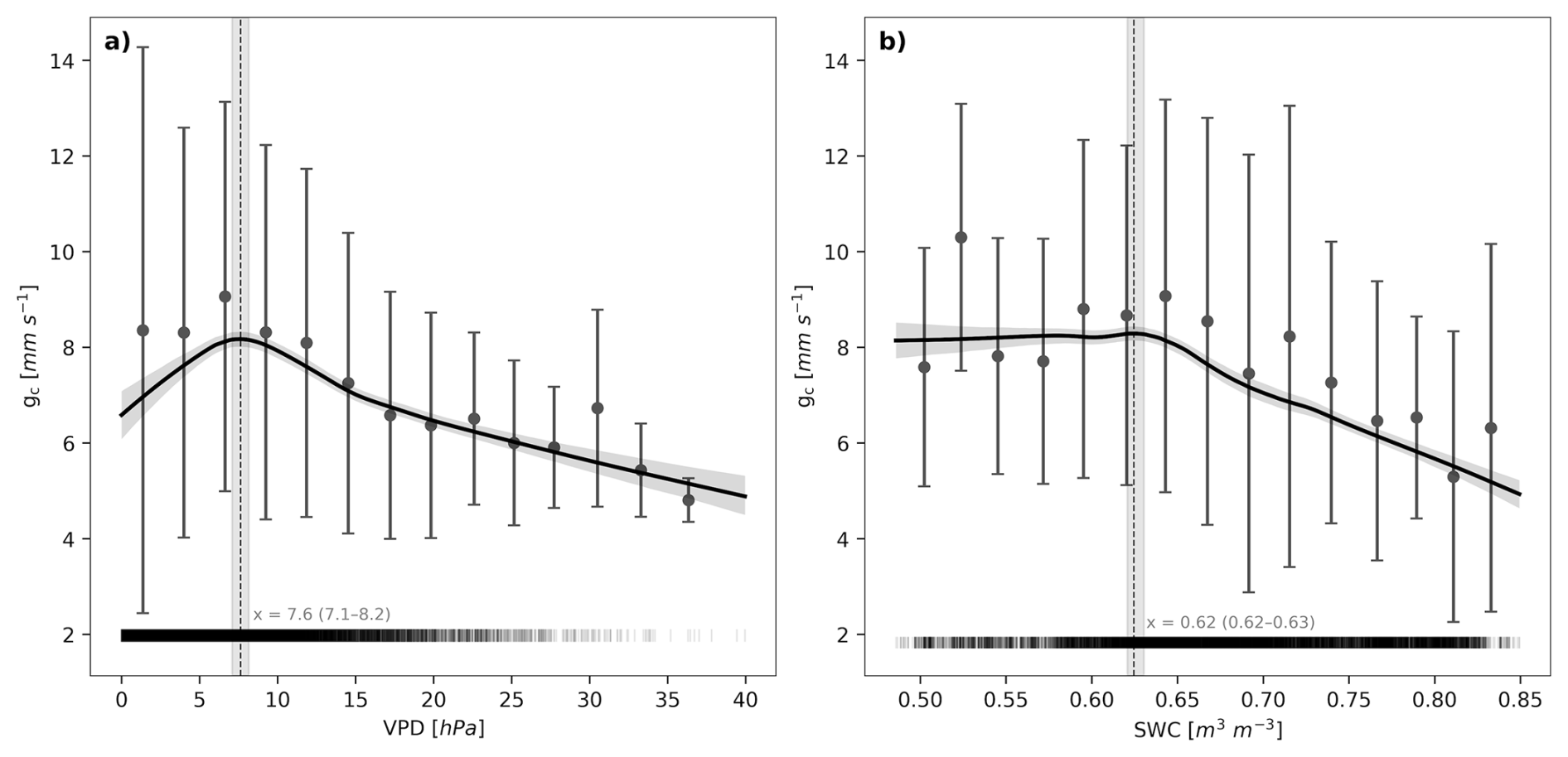
Figure 6Relationship between (a) canopy conductance (gc) and vapor pressure deficit (VPD) and (b) gc and soil water content (SWC). The data have a resolution of 30 min and were calculated using Eq. (2). Vertical lines in gray show mean and standard deviation for bins of the individual data points, in black a local polynomial regression. Gray area shows the 95 % confidence interval of the regression and its rightmost local maximum obtained using bootstrapping (n=1000). The vertical dashed line indicates the rightmost local maximum of the regression line. The lines on the x-axis show the data distribution. Data were restricted to the growing seasons and between 8 and 16 h.
4.1 Energy balance closure and data quality
This study provides the first analysis of biotic and abiotic drivers of LE fluxes in a peatland of the Central European lowlands. The energy balance closure was 83 %, which falls within the typical range reported for the EC method (70 %–90 %; Twine et al., 2000) and is above average for wetlands which is in average around 77 % (Nicolini et al., 2026). In our experimental setup, part of the residual imbalance likely arose from several well-known limitations of the EC method (Mauder et al., 2024). In peatland environments, advective and lateral transport of heat and water can represent a non-negligible component of the energy balance residual (Nicolini et al., 2026). The slightly larger energy balance closure on days with more than 2 mm P may be due to heat being added to the system by rain. In addition, large turbulent eddies with time scales exceeding the EC averaging period may contribute to the imbalance, as these motions are not fully captured by standard flux calculations. Further sources of imbalance include low pass filtering of water vapor by the intake tube of the gas analyzer, general measurement uncertainties, unaccounted energy storage (e.g., in soil or biomass), and errors introduced during data processing (Mauder et al., 2024; Nicolini et al., 2026). Outside the growing season, a considerable part of the energy balance component data is close to or below 0. In this range, unaccounted energy storage plays a greater role, which explains the lower value of the energy balance closure during the non-growing season. Daily averages allow for unaccounted energy storage to be averaged out to a large extent, which explains the slope of 0.99 for the energy balance closure when using daily average data. Despite these limitations, the observed closure indicates that the energy flux measurements are of sufficient quality to support robust analysis and interpretation.
4.2 Temporal dynamics of latent heat flux
When comparing turbulent energy fluxes in DE-Amv with similar sites (e.g., Gerling et al., 2019), during the warm season, LE generally dominates H, regardless of the site and its local climate. Gerling et al. (2019) found Bowen ratios < 1 in a central European mountainous peatland in July and August, similar to Gunawardhana et al. (2021) in an Australian peatland and Runkle et al. (2014) in a boreal peatland, where LE was several times higher than H. In the cold season, particularly in spring, B varies across regions: Alekseychik et al. (2017) and Runkle et al. (2014) observed LE > H during all measured months in boreal peatlands, while Gunawardhana et al. (2021) found B > 1 in Australian mountains, as in DE-Amv. In fall, the mountain valley bog in Australia had B < 1, whereas in DE-Amv, LE continued to exceed H. One possible explanation is that available energy goes more into LE than into H and that this ratio only reverses when LE is limited. Mamadou et al. (2016), for example, identified water availability in the soil as the main driver for changes in the Bowen ratio, whereby they investigated two different areas (cultivated area and woodland) in Northern Benin, where a dry and a rainy season exist. However, further research is needed to be able to make reliable statements about the underlying causes of the interaction between LE and H, particularly in the considered context of peatlands.
4.3 Drivers of latent heat flux
The GLSAR model enabled us to disentangle the individual effects on LE, which could not be achieved using correlation coefficients alone. The strong multicollinearity observed in the correlation analysis was largely driven by the seasonal co-variation with Rg. This issue was effectively mitigated through residualization, allowing for a more reliable assessment of biotic and abiotic drivers.
As typical for peatlands, DE-Amv is an energy-limited ecosystem (Table 2), with Rn influencing LE through two main mechanisms. First, it drives surface evaporation e.g., from soil. Second, it provides the energy necessary for biological activity, enabling vegetation to transpire and thereby further enhance LE. The pronounced influence of Rn on LE during the growing season likely reflects this overarching role. Outside the growing season, however, the residual aboveground vegetation in DE-Amv continues to shade the soil, limiting the direct impact of Rn on surface evaporation.
Although higher VPD physically promotes faster water evaporation, vegetation can counteract this through stomatal closure to prevent desiccation (Grossiord et al., 2020). Nevertheless, this physical relationship helps explain why VPD shows a strong influence on LE, particularly outside the growing season when stomatal regulation is largely absent. With global VPD expected to rise under climate change (Shekhar et al., 2024; Yuan et al., 2019), LE in DE-Amv is likely to be affected. Increases in VPD can enhance LE up to the point at which stomatal regulation limits transpiration, potentially offsetting or reversing this effect. While stomatal control has been well-documented in forest ecosystems under variable environmental conditions, our results – consistent with a limited number of studies (Speranskaya et al., 2024; Humphreys et al., 2006) – indicate that this mechanism also plays a significant role in peatland ecosystems. Consequently, the presence and variability of stomatal regulation across sites and vegetation types should be carefully considered in models of ecosystem energy, carbon, and water fluxes.
The decrease in gc with SWC above the threshold of 0.62 m3 m−3 SWC can be linked to the resulting stress on the woody vegetation (Bönsel and Sonneck, 2011). Although the driver analysis revealed a negative correlation between LE and SWC, this correlation was not significant during the growing season; this may be because VPD has a stronger influence on gc than SWC. The absence of a gc limitation for decreases in SWC further confirms that DE-Amv is energy-limited rather than water-limited, meaning that soil dryness does not limit transpiration in DE-Amv (Fig. 6a and b). These findings are consistent with previous research, which identified VPD as the dominant driver of LE and gc for areas with higher water availability (Zhang et al., 2024; Fu et al., 2022), such as peatlands. In contrast, compared to VPD, SWC dominates the limitation of LE in areas where water is limited (Zhang et al., 2024) and can contribute to intensifying heat extremes (Hirschi et al., 2011). Against this background, the results of this study highlight the importance of wetland ecosystems, their conservation, and their restoration. With 2023 and 2024, data includes the two years with highest and third-highest annual P since 2007, followed by the second-lowest annual P (2025) since 2007 (Deutscher Wetterdienst (DWD), 2022). The lack of LE limitations due to soil dryness despite the dry year of 2025 may be due to continued sufficient soil moisture but could also potentially be attributed to legacy effects from the preceding wet years (Du et al., 2024). Three years of data limit conclusions regarding changes in LE driver effect sizes during or after extreme events, even though the 95 % confidence intervals of the driver analysis are sufficiently narrow to provide robust results.
While meteorological factors such as Rn and VPD are frequently identified as the main drivers of LE (e.g., Gunawardhana et al. (2021) in a mountainous peatland), GPP is less often reported as a dominant driver. For example, Eichelmann et al. (2022) found that vegetation contributed 70 %–75 % to LE in California wetlands, and in this study as well, GPP, along with Rn, was the most important driver of LE. This discrepancy likely reflects the greater heterogeneity of vegetation compared to meteorological factors, both spatially and temporally. Furthermore, GPP is challenging to predict for the future: although it is expected to increase under climate change (Lu et al., 2024), the anticipated rise in extreme events, such as droughts, can alter the water balance and consequently GPP (Beniston et al., 2007). Therefore, further research is needed to understand how extreme events may modify the relative influence of different drivers on LE.
As the non-growing season is characterized by very low LE fluxes, very small influences such as that of Ta may not be statistically interpretable. Nevertheless, the effect size of VPD and WTD residuals are sufficiently strong (coefficients: VPD = 2.2, WTD = 2.5) to assume a genuine correlation between VPD and LE, as well as WTD and LE during the non-growing season.
gc peaked in summer, suggesting a delayed response of gc to increasing VPD. The relationship between gc and VPD observed here does not follow the exponential pattern reported in other studies (Runkle et al., 2014; Xu et al., 2021). This deviation may result from high variability in gc among species, leaf age, and environmental conditions (Song et al., 2022; Xu et al., 2021). For instance, Gobin et al. (2015) observed that Calluna vulgaris did not significantly close stomata under increasing VPD when soils were saturated, with similar results for Molinia caerulea, albeit at lower transpiration rates.
gc was modeled based on the assumption that during the growing season and without interception transpiration is approximately equal to ET. Here, we found no meaningful influence of misestimated proportions of transpiration on ET on the change points (Supplement Sect. S5).
This study demonstrates that LE in Central European drained bogs is primarily driven by a combination of Rn and GPP, with atmospheric demand (VPD) playing a crucial role, especially outside the growing season. The finding that stomatal regulation significantly limits transpiration during the growing season – even in water abundant peatlands – highlights that these ecosystems are more biologically controlled than previously assumed in simple energy driven models of LE. While the three-year dataset provides robust insights, longer-term monitoring is required to understand how extreme climatic events modify the relative influence of the identified drivers.
DE-Amv is planned for rewetting in the near future, which could alter peatland water balance, vegetation composition, canopy structure, and leaf area, thereby affecting LE. A more detailed evaluation of the contributions of individual functional plant groups – potentially by linking gc with phenological patterns – will be crucial for accurately predicting future LE dynamics and understanding the role of peatland ecosystems in regulating climate through energy fluxes. Overall, our results highlight that vegetation plays a significant and dynamic role in controlling LE in peatland ecosystems. Accurately accounting for species composition, functional traits, and stomatal regulation will be essential for predicting future LE dynamics and for understanding the contribution of peatlands to regional and global climate regulation.
Code is available upon request.
Eddy covariance and micrometeorological data are available via ICOS Carbon Portal under https://hdl.handle.net/11676/eRi-GMPnHz5rPsp425TmPiQv (Gharun and Behrens, 2026).
The supplement related to this article is available online at https://doi.org/10.5194/bg-23-8407-2026-supplement.
VF: formal analysis, methodology, software, visualization, writing (original draft preparation), writing (review and editing). NB: data curation, formal analysis, methodology, supervision, validation, writing (review and editing). MG: conceptualization, funding acquisition, methodology, project administration, resources, supervision, validation, writing (review and editing).
The contact author has declared that none of the authors has any competing interests.
Publisher's note: Copernicus Publications remains neutral with regard to jurisdictional claims made in the text, published maps, institutional affiliations, or any other geographical representation in this paper. The authors bear the ultimate responsibility for providing appropriate place names. Views expressed in the text are those of the authors and do not necessarily reflect the views of the publisher.
We would like to thank the two anonymous reviewers and the editor, Paul Stoy, for their constructive comments, which helped improve the manuscript. We are also grateful to all other discussion partners for their valuable input.
During the preparation of this work the author(s) used deepl.com in order to help with the translation from German into English. After using this tool/service, the author(s) reviewed and edited the content as needed and take(s) full responsibility for the content of the published article.
This open-access publication was funded by the University of Münster.
This paper was edited by Paul Stoy and reviewed by two anonymous referees.
Aitken, A. C.: IV. – On Least Squares and Linear Combination of Observations, Proc. R. Soc. Edinb., 55, 42–48, https://doi.org/10.1017/S0370164600014346, 1936.
Akaike, H.: A new look at the statistical model identification, IEEE T. Automat. Contr., 19, 716–723, https://doi.org/10.1109/TAC.1974.1100705, 1974.
Alekseychik, P., Mammarella, I., Karpov, D., Dengel, S., Terentieva, I., Sabrekov, A., Glagolev, M., and Lapshina, E.: Net ecosystem exchange and energy fluxes measured with the eddy covariance technique in a western Siberian bog, Atmos. Chem. Phys., 17, 9333–9345, https://doi.org/10.5194/acp-17-9333-2017, 2017.
Beck, P. S., Atzberger, C., Høgda, K. A., Johansen, B., and Skidmore, A. K.: Improved monitoring of vegetation dynamics at very high latitudes: A new method using MODIS NDVI, Remote Sens. Environ., 100, 321–334, https://doi.org/10.1016/j.rse.2005.10.021, 2006.
Beniston, M., Stephenson, D. B., Christensen, O. B., Ferro, C. A. T., Frei, C., Goyette, S., Halsnaes, K., Holt, T., Jylhä, K., Koffi, B., Palutikof, J., Schöll, R., Semmler, T., and Woth, K.: Future extreme events in European climate: an exploration of regional climate model projections, Climatic Change, 81, 71–95, https://doi.org/10.1007/s10584-006-9226-z, 2007.
Bönsel, A. and Sonneck, A.-G.: Effects of a hydrological protection zone on the restoration of a raised bog: a case study from Northeast-Germany 1997–2008, Wetlands Ecol Manage, 19, 183–194, https://doi.org/10.1007/s11273-011-9210-x, 2011.
Chen, T. and Guestrin, C.: XGBoost, Machinery, New York, USA, 785–794, https://doi.org/10.1145/2939672.2939785, 2016.
Cochrane, D. and Orcutt, G. H.: Application of Least Squares Regression to Relationships Containing Auto-Correlated Error Terms, J. Am. Stat. Assoc., 44, 32–61, https://doi.org/10.1080/01621459.1949.10483290, 1949.
Deutscher Wetterdienst (DWD): Climate Data Center: https://cdc.dwd.de/portal/202209231028/view1 (last access: 12 November 2026), 2022.
Dingman, S. L.: Physical hydrology, Third edn., Waveland Press Inc, Long Grove, Illinois, 643 pp., ISBN 10: 1-4786-1118-9, ISBN 13: 978-1-4786-1118-9, 2015.
Directorate-General for Environment: Natura 2000, European Commission, https://environment.ec.europa.eu/topics/nature-and-biodiversity/natura-2000_en (last access: 12 November 2026), 2024.
Dormann, C. F., Elith, J., Bacher, S., Buchmann, C., Carl, G., Carré, G., Marquéz, J. R. G., Gruber, B., Lafourcade, B., Leitão, P. J., Münkemüller, T., McClean, C., Osborne, P. E., Reineking, B., Schröder, B., Skidmore, A. K., Zurell, D., and Lautenbach, S.: Collinearity: a review of methods to deal with it and a simulation study evaluating their performance, Ecography, 36, 27–46, https://doi.org/10.1111/j.1600-0587.2012.07348.x, 2013.
Du, Q., Guan, Q., Sun, Y., Wang, Q., Zhang, J., Xiao, X., Liu, H., Yang, X., and Zhang, E.: Legacy effects of extreme drought and wetness events on mountain grassland ecosystems and their elevation dependence, J. Hydrol., 630, 130757, https://doi.org/10.1016/j.jhydrol.2024.130757, 2024.
Durbin, J. and Watson, G. S.: Testing for Serial Correlation in Least Squares Regression: I, Biometrika, 37, 409, https://doi.org/10.2307/2332391, 1950.
Durbin, J. and Watson, G. S.: Testing for Serial Correlation in Least Squares Regression. II, Biometrika, 38, 159–178, https://doi.org/10.1093/biomet/38.1-2.159, 1951.
Durbin, J. and Watson, G. S.: Testing for Serial Correlation in Least Squares Regression. III, Biometrika, 58, 1, https://doi.org/10.2307/2334313, 1971.
Eichelmann, E., Mantoani, M. C., Chamberlain, S. D., Hemes, K. S., Oikawa, P. Y., Szutu, D., Valach, A., Verfaillie, J., and Baldocchi, D. D.: A novel approach to partitioning evapotranspiration into evaporation and transpiration in flooded ecosystems, Glob. Change Biol., 28, 990–1007, https://doi.org/10.1111/gcb.15974, 2022.
Europäische Union: Standard-Datenbogen: DE3807301, in: Natura 2000-Gebiete in Nordrhein-Westfalen – Fachinformation – Listen der Natura 2000-Gebiete, Landesamt für Natur, Umwelt und Verbraucherschutz Nordrhein-Westfalen, https://natura2000-meldedok.naturschutzinformationen.nrw.de/natura2000-meldedok/de/fachinfo/listen/meldedok/DE-3807-301 (last access: 12 November 2026), 2021.
Fu, Z., Ciais, P., Prentice, I. C., Gentine, P., Makowski, D., Bastos, A., Luo, X., Green, J. K., Stoy, P. C., Yang, H., and Hajima, T.: Atmospheric dryness reduces photosynthesis along a large range of soil water deficits, Nat. Commun., 13, 989, https://doi.org/10.1038/s41467-022-28652-7, 2022.
Gerling, L., Weber, T. K., Reineke, D., Durner, W., Martin, S., and Weber, S.: Eddy covariance based surface-atmosphere exchange and crop coefficient determination in a mountainous peatland, Ecohydrology, 12, https://doi.org/10.1002/eco.2047, 2019.
Gharun, M. and Behrens, N.: ETC L2 ARCHIVE from Amtsvenn, 2023–2025, ICOS RI: https://hdl.handle.net/11676/eRi-GMPnHz5rPsp425TmPiQv (last access: 12 November 2026), 2026.
Gharun, M., Hörtnagl, L., Paul-Limoges, E., Ghiasi, S., Feigenwinter, I., Burri, S., Marquardt, K., Etzold, S., Zweifel, R., Eugster, W., and Buchmann, N.: Physiological response of Swiss ecosystems to 2018 drought across plant types and elevation, Philos. T. R. Soc. Lond., 375, 20190521, https://doi.org/10.1098/rstb.2019.0521, 2020.
Gobin, R., Korboulewsky, N., Dumas, Y., and Balandier, P.: Transpiration of four common understorey plant species according to drought intensity in temperate forests, Ann. Forest Sci., 72, 1053–1064, https://doi.org/10.1007/s13595-015-0510-9, 2015.
Grossiord, C., Buckley, T. N., Cernusak, L. A., Novick, K. A., Poulter, B., Siegwolf, R. T. W., Sperry, J. S., and McDowell, N. G.: Plant responses to rising vapor pressure deficit, New Phytol., 226, 1550–1566, https://doi.org/10.1111/nph.16485, 2020.
Gunawardhana, M., Silvester, E., Jones, O. A., and Grover, S.: Evapotranspiration and biogeochemical regulation in a mountain peatland: insights from eddy covariance and ionic balance measurements, J. Hydrol.: Regional Studies, 36, 100851, https://doi.org/10.1016/j.ejrh.2021.100851, 2021.
Harris, C. R., Millman, K. J., van der Walt, S. J., Gommers, R., Virtanen, P., Cournapeau, D., Wieser, E., Taylor, J., Berg, S., Smith, N. J., Kern, R., Picus, M., Hoyer, S., van Kerkwijk, M. H., Brett, M., Haldane, A., Del Río, J. F., Wiebe, M., Peterson, P., Gérard-Marchant, P., Sheppard, K., Reddy, T., Weckesser, W., Abbasi, H., Gohlke, C., and Oliphant, T. E.: Array programming with NumPy, Nature, 585, 357–362, https://doi.org/10.1038/s41586-020-2649-2, 2020.
Heijmans, M. M. P. D., van der Knaap, Y. A. M., Holmgren, M., and Limpens, J.: Persistent versus transient tree encroachment of temperate peat bogs: effects of climate warming and drought events, Glob. Change Biol., 19, 2240–2250, https://doi.org/10.1111/gcb.12202, 2013.
Hirschi, M., Seneviratne, S. I., Alexandrov, V., Boberg, F., Boroneant, C., Christensen, O. B., Formayer, H., Orlowsky, B., and Stepanek, P.: Observational evidence for soil-moisture impact on hot extremes in southeastern Europe, Nat. Geosci., 4, 17–21, https://doi.org/10.1038/ngeo1032, 2011.
Humphreys, E. R., Lafleur, P. M., Flanagan, L. B., Hedstrom, N., Syed, K. H., Glenn, A. J., and Granger, R.: Summer carbon dioxide and water vapor fluxes across a range of northern peatlands, J. Geophys. Res., 111, https://doi.org/10.1029/2005JG000111, 2006.
Hunter, J. D.: Matplotlib: A 2D Graphics Environment, Comput. Sci. Eng., 9, 90–95, https://doi.org/10.1109/MCSE.2007.55, 2007.
Karimi, S., Maher Hasselquist, E., Salimi, S., Järveoja, J., and Laudon, H.: Rewetting impact on the hydrological function of a drained peatland in the boreal landscape, J. Hydrol., 641, 131729, https://doi.org/10.1016/j.jhydrol.2024.131729, 2024.
Kettridge, N. and Waddington, J. M.: Towards quantifying the negative feedback regulation of peatland evaporation to drought, Hydrol. Process., 28, 3728–3740, https://doi.org/10.1002/hyp.9898, 2014.
Kottek, M., Grieser, J., Beck, C., Rudolf, B., and Rubel, F.: World Map of the Köppen-Geiger climate classification updated, metz, 15, 259–263, https://doi.org/10.1127/0941-2948/2006/0130, 2006.
Lafleur, P. M., Hember, R. A., Admiral, S. W., and Roulet, N. T.: Annual and seasonal variability in evapotranspiration and water table at a shrub-covered bog in southern Ontario, Canada, Hydrol. Process., 19, 3533–3550, https://doi.org/10.1002/hyp.5842, 2005.
Limpens, J., Holmgren, M., Jacobs, C. M. J., van der Zee, S. E. A. T. M., Karofeld, E., and Berendse, F.: How does tree density affect water loss of peatlands? A mesocosm experiment, PloS one, 9, e91748, https://doi.org/10.1371/journal.pone.0091748, 2014.
Liu, H., Rezanezhad, F., and Lennartz, B.: Impact of land management on available water capacity and water storage of peatlands, Geoderma, 406, 115521, https://doi.org/10.1016/j.geoderma.2021.115521, 2022.
Loescher, H. W., Hanson, C. V., and Ocheltree, T. W.: The Psychrometric Constant Is Not Constant: A Novel Approach to Enhance the Accuracy and Precision of Latent Energy Fluxes through Automated Water Vapor Calibrations, J. Hydrometeorol., 10, 1271–1284, https://doi.org/10.1175/2009JHM1148.1, 2009.
Lu, Q., Liu, H., Wei, L., Zhong, Y., and Zhou, Z.: Global prediction of gross primary productivity under future climate change, Sci. Total Environ., 912, 169239, https://doi.org/10.1016/j.scitotenv.2023.169239, 2024.
Mamadou, O., Galle, S., Cohard, J.-M., Peugeot, C., Kounouhewa, B., Biron, R., Hector, B., and Zannou, A. B.: Dynamics of water vapor and energy exchanges above two contrasting Sudanian climate ecosystems in Northern Benin (West Africa), J. Geophys. Res.-Atmos., 121, https://doi.org/10.1002/2016JD024749, 2016.
Massmann, A., Gentine, P., and Lin, C.: When Does Vapor Pressure Deficit Drive or Reduce Evapotranspiration?, J. Adv. Model. Earth Sy., 11, 3305–3320, https://doi.org/10.1029/2019MS001790, 2019.
Matos, K. A., Bowen, G. J., Good, S. P., and Allen, S. T.: Evapotranspiration Partitioning Across US Ecoregions: A Multi-Site Study Using Field Stable-Isotope Observations, Geophys. Res. Lett., 52, https://doi.org/10.1029/2025gl115367, 2025.
Mauder, M., Jung, M., Stoy, P., Nelson, J., and Wanner, L.: Energy balance closure at FLUXNET sites revisited, Agr. Forest Meteorol., 358, 110235, https://doi.org/10.1016/j.agrformet.2024.110235, 2024.
Miralles, D. G., Vilà-Guerau de Arellano, J., McVicar, T. R., and Mahecha, M. D.: Vegetation-climate feedbacks across scales, Ann. NY Acad. Sci., 1544, 27–41, https://doi.org/10.1111/nyas.15286, 2025.
Morgan, B. E., Araki, R., Trugman, A. T., and Caylor, K. K.: Ecological and hydroclimatic determinants of vegetation water-use strategies, Nature Ecology & Evolution, 9, 1791–1799, https://doi.org/10.1038/s41559-025-02810-8, 2025.
Nguyen, M. N., Hao, Y., Baik, J., and Choi, M.: Partitioning evapotranspiration based on the total ecosystem conductance fractions of soil, interception, and canopy in different biomes, J. Hydrol., 603, 126970, https://doi.org/10.1016/j.jhydrol.2021.126970, 2021.
Nicolini, G., Durden, D., Di Fiore, L., Florian, C., Sabbatini, S., Gielen, B., Iserbyt, A., Loubet, B., Mammarella, I., Mariotti, A., Beeck, M. op de, Slemmons, C., Trotta, C., Young, A., Chabbi, A., Feigenwinter, I., Heinesch, B., Kowalska, N., Mauder, M., Šigut, L., van der Molen, M., Bastos Campos, F., Berveiller, D., Brümmer, C., Cuntz, M., Domec, J.-C., Dumont, B., Fares, S., Gianelle, D., Jensen, R., Kalalian, C., Kljun, N., Lange, H., Limousin, J.-M., Lundin, E., Manco, A., Montagnani, L., Nemitz, E., Peichl, M., Rinne, E., Roland, M., Schmidt, M., Simioni, G., Thomas, A., Vincke, C., and Papale, D.: Bridging the Energy Balance Gap in Eddy-Covariance Measurements: Insights From Standardized Network Data, Glob. Change Biol., 32, e70892, https://doi.org/10.1111/gcb.70892, 2026.
Nijp, J. J., Metselaar, K., Limpens, J., Teutschbein, C., Peichl, M., Nilsson, M. B., Berendse, F., and van der Zee, S. E. A. T. M.: Including hydrological self-regulating processes in peatland models: Effects on peatmoss drought projections, Sci. Total Environ., 580, 1389–1400, https://doi.org/10.1016/j.scitotenv.2016.12.104, 2017.
Pastorello, G., Trotta, C., Canfora, E., et al.: The FLUXNET2015 dataset and the ONEFlux processing pipeline for eddy covariance data, Sci. Data, 7, 225, https://doi.org/10.1038/s41597-020-0534-3, 2020.
Pedregosa, F., Varoquaux, G., Gramfort, A., Michel, V., Thirion, B., Grisel, O., Blondel, M., Prettenhofer, P., Weiss, R., Dubourg, V., VanderPlas, J., Passos, A., Cournapeau, D., Brucher, M., Perrot, M., and Duchesnay, É.: Scikit-learn: Machine Learning in Python, J. Mach. Learn. Res., 12, 2825–2830, 2011.
Plotly Technologies Inc.: Collaborative data science, https://plot.ly (last access: 12 November 2026), 2015.
Rogiers, N., Eugster, W., Furger, M., and Siegwolf, R.: Effect of land management on ecosystem carbon fluxes at a subalpine grassland site in the Swiss Alps, Theor. Appl. Climatol., 80, 187–203, https://doi.org/10.1007/s00704-004-0099-7, 2005.
Runkle, B. R. K., Wille, C., Gažovič, M., Wilmking, M., and Kutzbach, L.: The surface energy balance and its drivers in a boreal peatland fen of northwestern Russia, J. Hydrol., 511, 359–373, https://doi.org/10.1016/j.jhydrol.2014.01.056, 2014.
Seabold, S. and Perktold, J.: Statsmodels: Econometric and Statistical Modeling with Python, Proceedings of the 9th Python in Science Conference, SciPy, 92–96, https://doi.org/10.25080/Majora-92bf1922-011, 2010.
Shekhar, A., Buchmann, N., Humphrey, V., and Gharun, M.: More than three-fold increase in compound soil and air dryness across Europe by the end of 21st century, Weather and Climate Extremes, 44, 100666, https://doi.org/10.1016/j.wace.2024.100666, 2024.
Song, L., Zhu, J., Li, X., Wang, K., Wang, G., and Sun, H.: Transpiration of Pinus sylvestris var. mongolica trees at different positions of sand dunes in a semiarid sandy region of Northeast China, Trees, 36, 749–762, https://doi.org/10.1007/s00468-021-02247-z, 2022.
Sonnentag, O., van der Kamp, G., Barr, A. G., and Chen, J. M.: On the relationship between water table depth and water vapor and carbon dioxide fluxes in a minerotrophic fen, Glob. Change Biol., 16, 1762–1776, https://doi.org/10.1111/j.1365-2486.2009.02032.x, 2010.
Speranskaya, L., Campbell, D. I., Lafleur, P. M., and Humphreys, E. R.: Peatland evaporation across hemispheres: contrasting controls and sensitivity to climate warming driven by plant functional types, Biogeosciences, 21, 1173–1190, https://doi.org/10.5194/bg-21-1173-2024, 2024.
The pandas development team: pandas-dev/pandas: Pandas, Zenodo [code], https://doi.org/10.5281/zenodo.3509134, 2025.
Truong, C., Oudre, L., and Vayatis, N.: Selective review of offline change point detection methods, Signal Processing, 167, 107299, https://doi.org/10.1016/j.sigpro.2019.107299, 2020.
Türk, H., Stumpp, C., Stockinger, M., and Benettin, P.: Tracking Event-Scale Precipitation Partitioning Reveals Comparable Roles of Event Characteristics and Seasonality in Shaping Precipitation Fate in a Forested Landscape, Hydrol. Process., 40, https://doi.org/10.1002/hyp.70466, 2026.
Twine, T. E., Kustas, W. P., Norman, J. M., Cook, D. R., Houser, P. R., Meyers, T. P., Prueger, J. H., Starks, P. J., and Wesely, M. L.: Correcting eddy-covariance flux underestimates over a grassland, Agr. Forest Meteorol., 103, 279–300, https://doi.org/10.1016/S0168-1923(00)00123-4, 2000.
Utikal, J. and Rückriem, C.: Maßnahmenkonzept: Natura 2000 Amtsvenn und Hündfelder Moor DE-3807-301, in: Natura 2000-Gebiete in Nordrhein-Westfalen – Fachinformation – Listen der Natura 2000-Gebiete, Landesamt für Natur, Umwelt und Verbraucherschutz Nordrhein-Westfalen, https://natura2000-meldedok.naturschutzinformationen.nrw.de/natura2000-meldedok/de/fachinfo/listen/meldedok/DE-3807-301 (last access: 12 November 2026), 2019.
van Rossum, G. and Drake, F. L.: Python 3 reference manual, Documentation for Python, Createspace Independent Pub, 244 pp., ISBN-10: 1441412697, ISBN-13: 978-1441412690, 2009.
Virtanen, P., Gommers, R., Oliphant, T. E., Haberland, M., Reddy, T., Cournapeau, D., Burovski, E., Peterson, P., Weckesser, W., Bright, J., van der Walt, S. J., Brett, M., Wilson, J., Millman, K. J., Mayorov, N., Nelson, A. R. J., Jones, E., Kern, R., Larson, E., Carey, C. J., Polat, ., Feng, Y., Moore, E. W., VanderPlas, J., Laxalde, D., Perktold, J., Cimrman, R., Henriksen, I., Quintero, E. A., Harris, C. R., Archibald, A. M., Ribeiro, A. H., Pedregosa, F., and van Mulbregt, P.: SciPy 1.0: fundamental algorithms for scientific computing in Python, Nat. Methods, 17, 261–272, https://doi.org/10.1038/s41592-019-0686-2, 2020.
Wilusz, D. C., Harman, C. J., and Ball, W. P.: Sensitivity of Catchment Transit Times to Rainfall Variability Under Present and Future Climates, Water Resour. Res., 53, 10231–10256, https://doi.org/10.1002/2017WR020894, 2017.
Wutzler, T., Lucas-Moffat, A., Migliavacca, M., Knauer, J., Sickel, K., Šigut, L., Menzer, O., and Reichstein, M.: Basic and extensible post-processing of eddy covariance flux data with REddyProc, Biogeosciences, 15, 5015–5030, https://doi.org/10.5194/bg-15-5015-2018, 2018.
Xu, J., Wu, B., Ryu, D., Yan, N., Zhu, W., and Ma, Z.: Quantifying the contribution of biophysical and environmental factors in uncertainty of modeling canopy conductance, J. Hydrol., 592, 125612, https://doi.org/10.1016/j.jhydrol.2020.125612, 2021.
Yu, Z. C.: Northern peatland carbon stocks and dynamics: a review, Biogeosciences, 9, 4071–4085, https://doi.org/10.5194/bg-9-4071-2012, 2012.
Yuan, W., Zheng, Y., Piao, S., Ciais, P., Lombardozzi, D., Wang, Y., Ryu, Y., Chen, G., Dong, W., Hu, Z., Jain, A. K., Jiang, C., Kato, E., Li, S., Lienert, S., Liu, S., Nabel, J. E. M. S., Qin, Z., Quine, T., Sitch, S., Smith, W. K., Wang, F., Wu, C., Xiao, Z., and Yang, S.: Increased atmospheric vapor pressure deficit reduces global vegetation growth, Science Advances, 5, eaax1396, https://doi.org/10.1126/sciadv.aax1396, 2019.
Zhang, Y., Liu, X., Wang, K., Zhang, D., and Liu, W.: Widespread Increasing Control of Water Supply on Evapotranspiration, Water Resour. Res., 60, https://doi.org/10.1029/2024WR038353, 2024.