
the Creative Commons Attribution 4.0 License.
the Creative Commons Attribution 4.0 License.
 | 20 Nov 2026
Evaluating GNSS-T VOD sensitivity to plant water dynamics, rainfall interception, and dew in a coniferous forest
Konstantin Schellenberg

Sinikka J. Paulus
Ronald Queck
David Chaparro
Oliver Binks
Maurizio Mencuccini
Sharath S. Paligi
Henrik Hartmann
Christiane Schmullius
Clémence Dubois
Thomas Jagdhuber
Monitoring forest canopy water is essential for understanding drought response and interception losses under climate change. At short timescales, canopy water is partitioned among internal plant water storage (Sp), rainfall interception (Si), and dew (Sd), which together regulate plant functioning, canopy evaporation, and precipitation partitioning, yet are rarely observed simultaneously. GNSS transmissometry (GNSS-T) has recently emerged as a low-cost, continuous, stand-scale method to observe L-band vegetation optical depth (VOD) from signal attenuation. However, interpreting GNSS-T VOD remains difficult because the signal integrates multiple water pools and is similarly affected by biomass, canopy structure, and measurement noise.
Here, we applied GNSS-T in a mature Picea abies stand in Tharandt, Germany, during the 2024 growing season to separate canopy water storage into Si, Sd, and Sp. Rainfall interception was simulated with the multilayer Penman-Rutter model CanWat and used to calibrate the empirical VOD to water storage relationship and to convert the GNSS-T noise floor into an equivalent storage detectability threshold. GNSS-T VOD tracked interception storage robustly and approximately linearly at both 30 min and event scales (), and modeled Si explained VOD variability better than gross precipitation alone. The inferred attenuation coefficient b was comparable in magnitude to reported L-band values and showed a seasonal variation, which we accounted for with monthly binned calibrations of b. Dew-related wetting signals were distinguishable in VOD and yielded plausible mean nightly amounts, while the largest predictions exceeded reported values and physical boundaries, which we attribute to residual noise in the VOD data. Diurnal changes in internal plant water storage were not directly detectable at sub-daily and daily scales, indicating that variations in Sp remained below the GNSS-T noise floor during the study period, as shown with trait-based estimates of maximum plant water loss.
This storage-versus-noise framework provides a practical way to benchmark the hydraulic sensitivity of GNSS-T across sites that differ in biomass, hydraulic strategy, and climate, and further highlights noise reduction as a prerequisite for plant-hydraulic applications. This study further promotes GNSS-T VOD as a robust monitoring instrument for resolving sub-event interception storage, a potential avenue for constraining hydrological models.
- Article
(4381 KB) - Full-text XML
-
Supplement
(4558 KB) - BibTeX
- EndNote


Forests link soil, vegetation, and atmosphere and are thereby the interface of the water, energy, and carbon cycles. Under ongoing climatic change, forests are exposed to increasing drought stress that can lead to tree mortality while shifting precipitation regimes can alter forest water supply onto the canopy and the soil (Hammond et al., 2022; Pendergrass et al., 2017). In this context, direct observation of forest water content gains increased attention (Konings et al., 2021) as it offers a way to connect process understanding across disciplines that have often developed separately, particularly hydrometeorology on the one hand and plant drought response on the other.
At canopy scale, forest water content is composed of functionally distinct but physically co-occurring pools. Internal plant water storage Sp sustains cell turgor, provides structural integrity, buffers transpiration, and is tightly linked to the water potential in the conduits that governs stomatal regulation and maintenance of hydraulic functioning (Nobel, 2020). Surface water storage, by contrast, is supplied intermittently by atmospheric inputs and includes rainfall interception Si and dew Sd or fog deposition on leaves and bark. These surface water pools directly influence canopy evaporation, throughfall, and the partitioning of precipitation into soil recharge and runoff (Van Stan et al., 2020). Together, Sp, Si, and Sd define the short-term water pools of the canopy. Yet, they are rarely assessed simultaneously, despite their joint dynamics that connect plant functioning with land-atmosphere energy and water exchange.
From the plant physiological perspective, internal water storage is of particular interest because the relative (to full hydration) water content of leaves and sapwood is functionally related to tissue water potential and thus to the availability of water for physiological processes (Martinez-Vilalta et al., 2019). Declining water potential triggers stomatal down-regulation, can lead to tissue conductivity loss, and even cause drought-induced tree mortality (Bartlett et al., 2012; Brodribb and McAdam, 2017; Tyree and Yang, 1990; Arend et al., 2021). Inferring plant water status and hydraulic status at the stand scale requires linking tissue water storage to the ecosystem level (Binks et al., 2024), however, the observational basis for such scaling remains scarce. Measurements of plant water status are still limited to mostly individual tree tissues and require labor-intensive sensors or destructive sampling, while geographically representative ecosystem-scale observations remain patchy (Novick et al., 2022; Restrepo-Acevedo et al., 2024). This hurdles currently limit monitoring of drought stress at the scale of forests and constrains the evaluation of land-surface and ecosystem models.
For hydrometeorology, information on canopy surface water pools is equally important. Rainfall interception stores a non-negligible fraction of precipitation on the surfaces of canopies, from where it can either drip to the forest floor or evaporate back to the atmosphere. The evaporated fraction can represent a substantial share of total precipitation and strongly affects the catchment water balance and water availability to the plants themselves (Klaassen et al., 1998). Small biases in the estimation of Si therefore propagate into uncertainties in soil recharge, runoff generation, and wet-canopy evaporation (Van Dijk et al., 2015). Dew can also contribute substantially to canopy water inputs, yet remains difficult to quantify, especially in forests where observations are sparse and no standard method exists (Tomaszkiewicz et al., 2015; Ritter et al., 2019). Established approaches for observing interception and dew often rely on residual water-balance methods or wetness sensors that suffer from limited spatial representativeness. Also, the eddy-covariance method that integrates a larger spatial footprint cannot precisely assess small water fluxes, especially during and after rain, and additionally suffers from energy closure errors (Dorigo et al., 2021; Zhong et al., 2022). As a result, the canopy surface water fluxes are still poorly constrained at plot-scale due to the complexity of the system and the lack of direct observations.
Microwave remote sensing is particularly promising in this regard because vegetation water interacts directly with microwave radiation (Ulaby and El-rayes, 1987). As microwaves propagate through the canopy, they are attenuated by absorption and scattering, and these losses can commonly be described by vegetation optical depth, VOD (Jackson and Schmugge, 1991; Frappart et al., 2020). Owing to their long wavelengths, microwave observations provide a measure of canopy water status integrated over large parts of the vertical forest volume. VOD has been linked to vegetation water content and, when accounting for biomass variability, to plant hydraulic status and water potential across satellite and plot scales (Momen et al., 2017; Holtzman et al., 2021; Rao et al., 2019; Meyer et al., 2019; Chaparro et al., 2024; Jagdhuber et al., 2025). At the same time, interpretation remains challenging because VOD responds not only to water content, but also to biomass, canopy structure, viewing geometry, and the coexistence of internal and surface water pools (Xu et al., 2021).
Recently, GNSS-Transmissometry (GNSS-T), has emerged as a low-cost plot-scale up to stand-scale approach for observing canopy attenuation from the L-band signals transmitted by global navigation satellites (Humphrey and Frankenberg, 2023). By comparing above- and below-canopy signal strength, GNSS-T estimates canopy transmissivity and derives VOD from the attenuation caused by vegetation. The principle had been demonstrated before by several groups: Rodriguez-Alvarez et al. (2012) estimated vegetation water content from the attenuation of GNSS signals, Liu et al. (2017) predicted boreal forest attributes from GNSS signals at low cost, Zribi et al. (2017) tracked daily variations of the water content of a sunflower canopy with low-cost GPS receivers, and Camps et al. (2020) retrieved L-band VOD from transmitted GNSS signals with a single dual-polarization antenna. Guerriero et al. (2020) showed that stand structure and biomass vary with GNSS-T VOD. GNSS-T offers several advantages, as it is affordable enough for broader deployment and measures continuously. A further advantage of GNSS-T is that it senses canopy attenuation directly. In contrast, downward-looking radiometric systems derive VOD indirectly from radiative transfer inversion, which introduces additional uncertainty through the need to separate the soil contribution. For these reasons, GNSS-T has strong potential to bridge the gap between point-scale hydraulic observations and ecosystem-scale monitoring (Feldman, 2024; Restrepo‐Acevedo et al., 2026).
Up to date, however, the interpretation of GNSS-T VOD still is ambiguous to some degree. Existing studies commonly indicate sensitivity to water limitation and canopy water dynamics, but they do not agree in whether GNSS-T signals can reliably capture diurnal variations in plant water status (Humphrey and Frankenberg, 2023; Yao et al., 2024; Burns et al., 2025). This matters because sub-daily variations in VOD can be used to disentangle short-term hydraulic responses from the low frequency effects of seasonal biomass variation (Konings et al., 2021). Physiologically, the diurnal cycle of vapor pressure deficit (VPD) that regulates stomatal conductance and drives depletion and replenishment of internal water stores, makes these dynamics a sensitive indicator of water stress (Nelson et al., 2018). Diurnal GNSS-T VOD variations have been observed in broadleaf forests, but not consistently in evergreen needleleaf systems. This contrast may arise from differences in canopy structure, above-ground biomass, hydraulic strategy, and climatic forcing among sites, as well as from substantial GNSS-T noise that obscures weak sub-daily signals (Humphrey and Frankenberg, 2023). Therefore, gaining progress requires identifying which canopy water pools GNSS-T captures, with what sensitivity, and under which detectability constraints.
In this study, we approach this challenge by treating GNSS-T VOD as an integrated observation of forest canopy water content of which we explicitly separate its likely contributors into rainfall interception Si, dew Sd, and internal plant water storage Sp. The key idea is that rainfall interception provides the strongest wetting signal in the canopy. We use modeled interception storage to calibrate the empirical relationship between VOD and canopy water storage, and then use this relationship to translate the GNSS-T noise floor into an equivalent storage detectability threshold. This allows us to assess not only whether GNSS-T tracks surface water, but also whether weaker canopy water signals such as dew formation and diurnal plant-water dynamics are large enough to be observed, despite the presence of GNSS-T noise.
GNSS-T receives signals from within a field-of-view that has the shape of an inverted cone whose tip is the ground receiver, the cone bottom area located at the forest canopy top. The volume of this cone (“footprint”) is systematically biased towards the top-canopy, as the cone volume increases quadratically towards the top. This bias affects comparisons of water pool estimations from GNSS-T VOD with other methods based per ground-area, like meteorological variables, eddy covariance or radiometry. Previous studies have acknowledged the problem of footprint area size calculations (Burns et al., 2025), however, they have not yet analyzed the influence of the bias on the correlation with water pools. For this reason, we test of the correlation of water pool with GNSS-T VOD decline when using a column-type instead of a cone-type footprint.
To this end, we conducted a GNSS-T experiment in a mature Picea abies stand in Tharandt, Germany, during the 2024 growing season. This site combines high biomass and substantial interception capacity, which may be indicative of high Sp and Si signals. We use ancillary data to separate canopy water pools, including throughfall observations, a physically based interception model tailored to the site fluxes, and sapflow-based plant water dynamics. We first quantify the sensitivity of GNSS-T VOD to interception storage and evaluate this relationship against a 3-dimensional multilayer Penman-Rutter model of canopy wetting and drying. Because VOD integrates multiple canopy water pools, rainfall-driven interception signals may be partly modified by concurrent plant water uptake, which we discuss. We then assess whether dew-related VOD changes are detectable and whether inferred dew amounts are plausible in the context of reported forest values. Finally, we compare the magnitude of expected variation in Si, Sd, and Sp against the empirically estimated GNSS-T noise threshold across temporal aggregation scales. In doing so, we evaluate GNSS-T as a method to observe whole-canopy water content and to connect canopy hydrometeorology with plant drought response at stand scale.
Here, we address the question whether GNSS-T can move beyond being a generic and integrated proxy for vegetation wetness and instead provide a physically interpretable measure of forest canopy water content. If successful, such an approach would offer a practical route to monitor both transient surface wetness and functionally relevant plant water dynamics within one integrated observational framework.
In our study, we test the following hypotheses:
- H1.
GNSS-T VOD responds positively and linearly to rainfall interception storage Si at Tharandt at both 30 min and event scales, and modeled Si explains VOD variability better than gross precipitation.
- H2.
Accounting for the inverted-cone footprint of GNSS-T yields a stronger correlation with Si than comparing VOD against Si of an equivalent column.
- H3.
Dew and non-dew storage Sd can be distinguished in GNSS-T VOD, and if yes, predicted dew amounts from VOD compare well with literature values, and the physical condensation limits.
- H4.
The diurnal variability in plant water storage Sp can be observed, i.e. surpasses the VOD noise threshold, with GNSS-T VOD at sub-daily scales given the high water turnover expected in the Tharandt forest ecosystem.
2.1 Site description
The experiment is set at the environmental observatory station Tharandt (50°57′49′′ N, 13°34′01′′ E; 380 m a.s.l.) which lies ∼ 25 km southwest of Dresden, Germany, within the eastern sector of a 60 km2 forest. The climate is transitional sub-oceanic/sub-continental: convective rainfall dominates in summer, weaker frontal systems in winter. Mean annual precipitation is 820 mm and mean air temperature is 7.6 °C for 1981–2010 (Grünwald and Bernhofer, 2007; Grunicke et al., 2020).
The forest around the flux tower, which host the GNSS-T reference antenna and eddy-covariance (EC) sensors (ICOS station name DE-Tha, Grünwald et al., 2025), is a Picea abies stand embedded in a landscape that is ∼ 87 % evergreen coniferous and ∼ 13 % deciduous (Fig. 1). The stand structure in the GNSS focal footprint is characterized by 477 trees ha−1, above-ground biomass of 213 t ha−1, and canopy heights ranging between 29 and 33 m (Queck et al., 2016), and was planted in 1887. This mature, evergreen spruce canopy offers three advantages for the purpose of this study: (i) It has high, seasonally stable biomass and weak leaf phenology, as indicated by low variability in PAI throughout the year, as evident from Grunicke et al. (2020, Fig. 3) that show 13 % intra-annual variability (max 3.9, min 3.38) in the period after the last thinning in 2011. This minimizes confounding biomass effects in the VOD data and simplifies its interpretation. Then, (ii), dense, needle-rich crowns provide a large surface area and thus a high interception storage capacity, larger than broadleaf species (Pflug et al., 2021, Table 6), resulting in a wide dynamic range for intercepted water storage. Also, (iii), the high stand biomass can retain large quantities of plant internal water, ensuring high L-band attenuation.
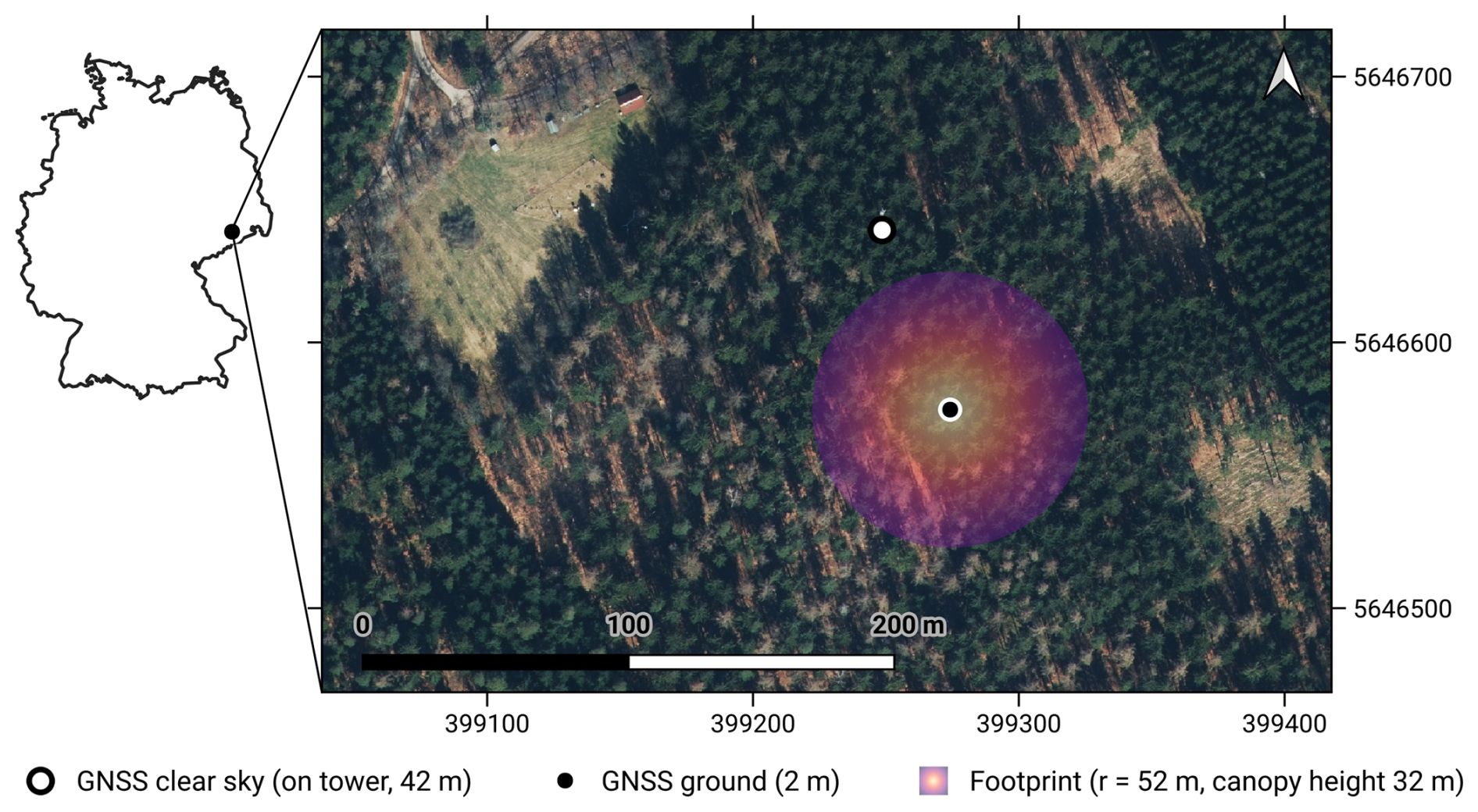
Figure 1Location of GNSS antennas at the research site Tharadt, Germany. The ground antenna is situated on the forest floor (black dot); the clear-sky reference antenna is mounted on top of the eddy covariance tower (white dot). The footprint of the GNSS is illustrated by the circle where the outline represents the maximum extent of the footprint at canopy height; the color hue indicate the increasing fraction of forest volume falling into the GNSS footprint when moving toward the antenna. For a 3-D visualization of the vegetation material in the footprint, the reader is referred to Figs. S1 and S2 in the Supplement. Map source: True color composite airborne image by Landesamt für Geobasisinformation Sachsen (GeoSN).
The study period covers the frost-free growing season (25 April 2024–15 October 2024), confined by the operational period of canopy throughfall measurements used for the CanWat model which do not operate during freezing periods.
2.2 GNSS-T Vegetation Optical Depth
For the GNSS-T setup, we used two identical low-cost SparkFun SPK6618H antennas, connected with 3 m coaxial cables to u-blox ZED-F9P receiver boards; one positioned above-canopy (clear-sky reference) and one below-canopy (ground) (Humphrey and Frankenberg, 2023). The ground antenna was placed below the canopy in an area with > five m distance from the closest trunk to avoid signal occlusion; its height is two m above ground mounted on a steel pole. We attached the open-sky reference antenna to the top of the EC tower at 42 m height with no lightning protector in view that might produce interferences. The receiver logs the carrier-to-noise ratio (, commonly called SNR) data via NMEA 4.10 messages for all available GNSS constellations (GALILEO, GPS, BeiDou, GLONASS) and frequency bands, and sends them to a micro controller for storage which are altogether stored in a weather-proof capsule. We used GNSS signals from all available bands which are clustered in the lower (1.16–1.24 GHz; bands L2, E5, B2 of GPS, GALILEO, and BeiDou, respectively) and upper L-band (1.56–1.59 GHz; bands L1, E1, B1). The NMEA format only allows for a 1 dB radiometric resolution which we aimed to enhance using a very high observation frequency of 1-second intervals. The GNSS-T footprint and the visualization of the over-representation of the top-canopy layers by the viewing geometry are displayed in Figs. 1, S1, and S2.
To obtain the attenuation signal, we calculate the ratio to the reference receiver. This way, influences due to antenna gain pattern, satellite power variability, and atmospheric influences in the ground antenna SNR are accounted for. The remaining signal is then only a result of the wave interaction in the canopy (Humphrey and Frankenberg, 2023):
The attenuation ΔSNR (dB) is then converted to transmissivity γ, and path-length–corrected the Lambert-Beer's law (Ulaby and Long, 2014, Eq. 6.61):
where θ (rad) is the incidence angle. We only use data from incidence angles < 60° to limit multi-path scattering that potentially violate the assumption of medium homogeneity in Eq. (3); the hemispheric grid resolution is 1°.
We calculate the time series by integrating data from all satellites in the hemisphere over a 30 min interval using the biomass correction proposed by Humphrey and Frankenberg (2023) to reduce spurious artifacts from the sparse hemispheric sampling of GNSS over an inhomogeneous canopy. They showed an effective noise suppression at sub-daily scales by normalizing VOD with the combined long-term “baseline” mean of all satellites that cross a sky-sector. While effective, we found that pooling all satellite for the baseline mean produces aliases in the time series. Instead, we then enhanced the approach by calculating baselines for each satellite and sky-sector, yielding a more consistent VOD time series in terms of higher temporal autocorrelation and lower standard deviation, i.e. less abrupt signal changes and less noise in the final VOD time series (Figs. S3–S4). Both formulations are given in Appendix A2. Also, we excluded data from GLONASS satellites as they were found to add sudden extrema in the time series (also Figs. S3–S4), as documented in Schellenberg et al. (2024). Note, that those adjustments might not be generalizable to other GNSS-T setups with different receivers but proved effective in our data set.
VOD is influenced by the temperature of the canopy (Ulaby and El-rayes, 1987), which has an effect on global VOD retrievals (Zhao et al., 2024). For GNSS-T VOD, this effect could be shown under extreme heat gradients (10–45 °C) in a dry ecosystem (Humphrey and Frankenberg, 2023), while effects in temperate ecosystems remain low, as shown by Kesselring et al. (2026). Since Tharandt is close to conditions in the latter experiment, we assume temperature effect of only marginal influence to this study. Also, wetness on the GNSS receiver from dew or rain might add noise to VOD. However, Humphrey and Frankenberg (2023) could show that wetness of the antenna did not have an effect on the VOD signal in their experiment. We, therefore, assume the impact to be low in this study.
2.3 VOD noise threshold
GNSS-T VOD signals are inhibited by a random noise component and a repetitive, deterministic noise pattern. The deterministic noise is known to be caused by the combination of under-sampling over a heterogeneous canopy caused by the satellite tracks and the canopy distribution (Humphrey and Frankenberg, 2023), while the random noise is related to the receiver and the wave transmission itself. Of these two components, only the orbit-induced deterministic part is explicitly accounted for, through the per-satellite baseline normalization described in Appendix A2. Everything that remains is collapsed into a single term, which therefore contains the random noise of the receiver and of the wave propagation, and may still include residual deterministic structure that this correction does not capture. We consequently treat it as an effective noise term rather than as a purely random one, and do not claim that the two components are fully separated. To understand the impact of noise on the sensitivity of GNSS-T VOD, we extract a noise time series ϵ(t) as
To estimate ϵ(t), we (i) mask out all periods with dew or interception, (ii) compute a 14 d centered running median VODtrend(t) to capture low-frequency variability that acts as a representation of the above-ground biomass (AGB), changes in canopy structure and long-term Sp trends, and (iii) estimate the plant water fraction of the signal by fitting a stationary diurnal Fourier series on dry periods as a rough proxy for plant-water dynamic (Schellenberg et al., 2024); the specification of this fit, its cross-validation, and the resulting decomposition are given in Appendix A3 and Fig. S16. The noise threshold ϵ is then
Note that we assume that instrument ϵ is similar between wet and dry conditions, however, we did not verify this, e.g. if wetness on the antennas modulate noise. Here, we follow Humphrey and Frankenberg (2023) who could not find a measurable effect of wet-states on VOD.
Now, we define a threshold of detectability by the SNR>3 dB rule that is widely used in signal processing (Harris et al., 1974). If a signal (here: water storage) exceeds the power of the underlying noise by double, it is referred to as “detectable”. The threshold δ is calculated by transforming SNR=3 dB from decibels to linear scale (), converting to the amplitude (), and multiply by the signal noise, expressed here as mean root mean square of the noise time series:
The RMS is calculated by
To express the threshold metric in mm, so that it can be compared to interception amounts, a linear model is used:
linking VOD to vegetation water content (VWC, mm) via the attenuation coefficient b (Jackson and O'Neill, 1990). Now, , where the b-parameter is obtained from the empirical VOD–Si correlation that will be described in Sect. 2.4. Since δ is a property of the instrument and its noise, we use the time-independent, season-wide fit over all observations with b=0.131 VOD mm−1 (Table 4). Note, that δ is subject to the VOD–Si relationship that varies throughout the season. Refitting VOD–Si in monthly bins gives δ3 dB between 0.37 and 0.45 mm at 30 min resolution, i.e. about ±10 %. Not included is the calibration uncertainty of the CanWat storage (24 %, 1σ), which is described in Sect. 2.4. As δ serves as a common reference for all storage terms and aggregation windows, we do not propagate the calibration uncertainty of b into it, but acknowledge it here.
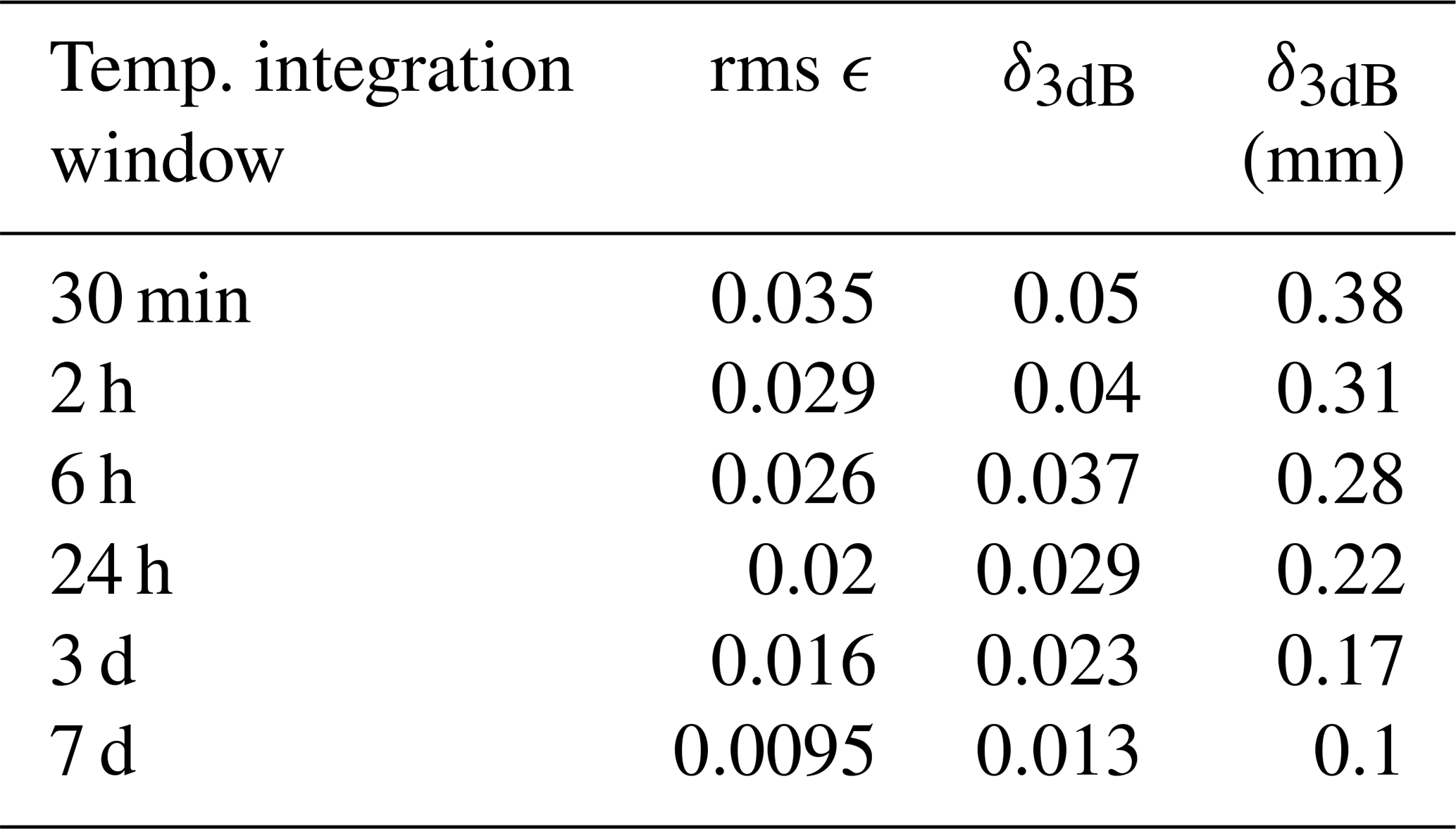
Table 1GNSS-T VOD noise threshold ϵ and the associated detectability threshold δ following the 3 dB rule, calculated over a range of temporal aggregation windows, so δ is a season-wise fit.
Two aspects of Eq. (8) deserve comment. First, we express VWC in mm rather than in the more conventional kg m−2. Both are numerically equivalent for water, and we chose mm because the quantities that VOD is compared against in this study, interception and dew, are meteorological water depths, so that one unit is kept throughout the manuscript. We note that VWC conventionally refers to the water held inside the vegetation, whereas we apply Eq. (8) to the total canopy water content, including the water held on the surface.
Second, this application assumes that surface water attenuates the L-band signal in a similar way as internal water. Water in vegetation can be separated into bound water, which is chemically held to the organic material, and free water, which resides either within the tissue or as surface water on leaves and bark. Ulaby and El-rayes (1987) showed that the two differ in their dielectric behavior and therefore in their attenuation properties, and that the volume fraction of bound water rises steeply at low moisture but approaches a plateau as the material becomes wetter (their Fig. 5). Consistently, Romanov (2025) found the slope of VOD against VWC to become non-linear once the ratio of bound to free water changes. Assuming that the trees at Tharandt did not suffer excessive drought stress, the bound-water fraction would be approximately stable, so that the variability of VOD reflects the absolute amount of water present, whether bound or free, internal or on the surface. Here, it is a necessary and pragmatic assumption and deserves dedicated testing, especially with respect to GNSS-T measurements.
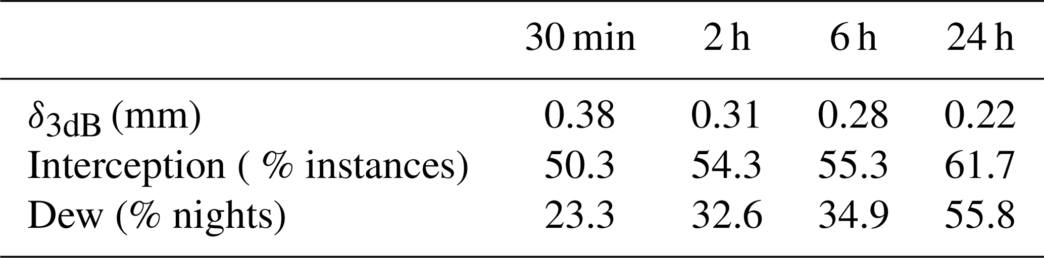
We test the influence of temporal integration windows as way to suppress noise in VOD data and calculate δ using the temporal rolling mean operation for 30 min, 2, 6, 24 hours, and 3, 7 days. We report that δ decreases from 0.38 to 0.22 mm with temporal aggregation from 30 min to daily resolution, and to 0.10 mm at weekly resolution (Table 1). Signal aggregation therefore critically influences which changes to the canopy water storage will be detectable or obfuscated by noise.
2.4 Rainfall interception
We used the 3-dimensional interception model CanWat to simulate canopy water storage Si in a grid of voxels covering the GNSS-T footprint (Queck, 2025, Model available on GitHub: https://github.com/Ron-Q/CanWat). CanWat is based on the conceptual framework established by Rutter et al. (1971) using the Penman-Monteith approach (Monteith and Unsworth, 2013), and has been applied to model interception in Tharandt (Fischer et al., 2026). The interception scheme implements these approaches as a vertical cascade of storages, the water balance of which is solved in each voxel with an adaptive fourth-order Runge–Kutta integrator. The canopy water balance is written as , where the incoming flux Pi combines the precipitation intercepted and the drainage from the voxels above, and the outgoing fluxes are evaporation E and drainage D. Earlier studies have shown that stemflow is negligible in rough-barked species, such as Picea abies in Tharandt (Cisneros Vaca et al., 2018), so we disregarded it in this study. Gaps in the canopy allow for free throughfall and are modeled using an 3-dimensional array of plant area density from terrestrial laser scanning with a resolution of 1 m3.
The wetting of the plant surface controls a resistance network that divides the available energy between transpiration and evaporation, via the Penman-Monteith equation. Within-canopy wind speed is provided by a mixing-length wind module, net and shortwave radiation by a radiative transfer scheme, and air temperature and water vapor pressure by vertical interpolation of profile measurements, so that a full local energy balance can be evaluated for each voxel. During and after rainfall, transpiration T is calculated in the same framework, using shortwave radiation to derive a canopy conductance and thereby partitioning available energy between intercepted water evaporation and transpiration. T will be used to infer the plant water balance with sapflow as input (Sect. 2.6.1). The resistance network follows the formulations of Jarvis (1976) and Stewart (1988) and was parameterized with eddy-covariance data from Tharandt in a series of earlier studies (Peters et al., 2003; Queck, 2004; Pruskowsky et al., 2005; Fischer et al., 2023). In its one-layer form, Fischer et al. (2026) evaluated the model against in-canopy water balance measurements from interception chutes and obtained R2>0.85; leaf width, stomatal conductance, and maximum interception storage capacity are taken from that study. Transpiration itself was not validated against eddy-covariance measurements in the present setup, so that its error cannot be quantified here.
Drainage follows an exponential storage–discharge relation. It is negligible while Si is below the voxel's storage capacity (mean canopy saturation capacity Smax=2.92 mm, from Grunicke et al., 2020), but increases exponentially once this threshold is exceeded. During the drying process, Si decreases, slowing down evaporation from the shrinking reservoir and would eventually reduce it to infinitesimally small amounts. To ensure a realistic full dry-down, the drying process is enforced below a threshold of 0.01 mm which also defines the end of a precipitation event. Storage above this is referred to as “wet canopy”.
All meteorological input variables and sensors used to drive the 3-D interception model are measured on the Tharandt scaffolding tower and summarized in Table A1.
To quantify the sensitivity of GNSS-T VOD to interception, we relate VOD to the modeled canopy interception storage Si from CanWat by fitting an ordinary least squares regression over all periods classified as wet-canopy conditions (Fig. 2), in the form of
in analogy to Eq. (8). The regression is fit without an intercept, assuming that in the absence of intercepted water (Si=0 mm), the interception-related contribution to VOD is zero; accordingly, R2 is computed as the squared Pearson correlation between observed and predicted VOD, . Physically, b (VOD mm−1) encapsulates how much canopy attenuates microwaves per unit intercepted rain water. It depends on canopy structure, incidence angle, and wavelength. The fitted slope is the effective bulk b-parameter that integrates over the distribution of GNSS-T incidence angles (Van de Griend and Wigneron, 2004). Note that Si is, by definition, the liquid water held on the canopy surface and therefore independent of the instantaneous rainfall rate, so that b is not a function of rainfall intensity. In addition, we compare Si estimates of the cone footprint of GNSS with an equivalent column that has the same base radius to test if effects of sensing volume will propagate into the sensitivity of VOD to Si when moving the domains. Unless stated otherwise, all water storage terms reported in this study are confined to the cone subset and expressed per unit ground area, obtained by projecting the 3-D cone volume onto the ground.
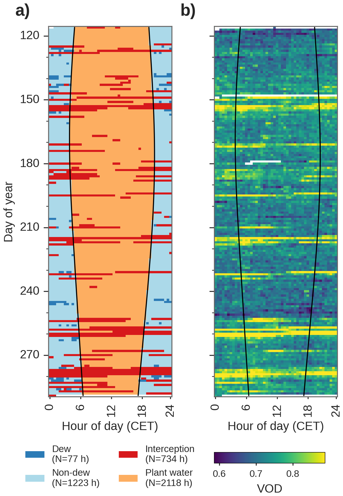
Figure 2Diurnal and seasonal classification of dominant water flux used throughout this study: Dew and non-dew nighttime reference, rainfall interception, and plant water (a); Diurnal and seasonal dynamics of GNSS-T VOD (b). The solid lines indicate sunset and sunrise.
For each rain event, the VOD data series is calculated as difference from the immediate pre-event (dry) conditions to remove biomass effects as previously described in Sect. 2.7.
Equation (9) assumes b to be a constant property of the canopy, invariant of phenology. However, intrinsic structural re-configurations of the canopy that determine its water-holding properties are expected to take place with progressing season due to leaf aging and climate responses, e.g. leaf-to-wood ratio, leaf orientation, or canopy shape. We therefore fit additional relationships with monthly bins in the form of VOD=b(month) Si. We chose per-month binning to represent the main phenological phases in this forest ecosystem, and only consider months covering more than one week of the study period, so that 25–30 April is excluded. The season-wide b is used to convert the noise threshold into millimeters (Sect. 2.3), whereas b(month) is applied as a monthly step function wherever VOD is converted into a water storage, in particular for quantifying the dew yield in Eq. (11).
The interception estimates from CanWat carry an additional uncertainty beyond the sampling error of the regression. Grunicke et al. (2020, Table 9) reported an RMSE of 0.5 mm for the model across a 7-year study period, which corresponds to a normalized error of %. Since this validation refers to throughfall rather than to canopy storage, we assume that the relative accuracy of the model transfers to Si, both being governed by the same storage capacity, drainage and evaporation parameterization. We take the RMSE as a conservative estimate of one standard deviation of this relative error so that to first order, and combine it with the ordinary least squares sampling error of the slope, SEOLS, in quadrature to calculate the 95 % confidence interval, CI95:
All uncertainties of b reported in the main text, for the season-wide fit as well as for b(month), follow Eq. (10) and therefore contain both terms. For comparability with the preprint version of this study, the corresponding figures carrying the OLS sampling error alone are provided in the supplement (Figs. S13–S15), and both intervals are listed side by side in the Supplement Table S2.
2.5 Dew formation
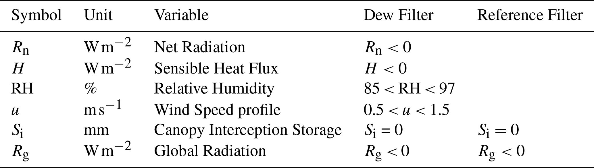
We test the sensitivity of VOD to the occurrence of dew by comparing nighttime periods with a high probability of dew formation with reference periods without dew formation. In principle, dew forms when the leaf surface temperature cools below the dew point, and the air at the leaf boundary layer is sufficiently humid (Monteith, 1957). We rely on a set of hydrometeorological filter instead of energy-balance model derived estimates since the latter has shown to carry only limited prediction power for dew events (Sibley et al., 2022). The key drivers of dew formation are radiation Rn, atmospheric humidity RH and wind u. Using those observation, we define a dew formation thresholds that is conservative per design in order to reduce false positives.
We define dew formation periods as nighttime conditions in which radiative cooling (Rn<0 W m−2) occurs and the canopy is cooler than the air (H<0 W m−2). Ritter et al. (2019) found dew occurring at atmospheric relative humidity (RH, %) as low as 75 % in some of in total 30 sites. They attributed their findings to the mismatch between the measurement sensor location and the actual temperature at the leaf boundary layer. Conditions close to vapor saturation (i.e. fog) reduce dew formation due to energy re-emission by vapor (Wærsted et al., 2017). Therefore, we chose a boundary of RH of 85 < RH < 97 % to allow for lower saturation, and to avoid fog (Paulus et al., 2022). We exclude periods of canopy interception using Si from the CanWat model. Within-canopy wind speed was restricted to m s−1, allowing some turbulent exchange to renew the vapor gradient at the leaf surface but excluding very calm or strongly ventilated conditions that suppress canopy cooling (Beysens, 2006; Ritter et al., 2019). Periods that do not meet the conditions summarized above are used as nocturnal reference. All variables and thresholds for both the dew filter and the nocturnal reference filter are summarized in Table 2.
Table 2Hydrometeorological filters defining dew conditions and reference night-time windows. Confounding hydrological variability are excluded for both filters, including rain interception and any daytime conditions to suppress change in plant water due to transpiration. Details on instrumentation is found in Table A1.
To evaluate the effect of dew on VOD, we performed a logistic regression with binary response of dew and non-dew conditions. To exclude confounding biomass and plant water, we use the VOD residual signal, ϵ, which is calculated in Eq. (5). In the logistic regression, the sample set for the binary response model is highly skewed (dew: 77 h, no dew: 1223 h), which can introduce bias toward the larger set. To alleviate this, we randomly down-sampled the no-dew observations to match the size of the dew set. Then, we estimated the mean bootstrapped coefficients (200 repetitions). Then, the predicted dew yield is built on the fit of VOD to rain interception storage
as derived from Eq. (8), where ϵ(t) is the VOD noise time series, and b(month) for the cone geometry is fit individually for each month from the VOD–Si relationship (see Table S2 for details).
To calculate nocturnal dew yields, we sum all observations per night, regardless of their sign (positive or negative), to generate an unbiased estimate of the mean yield, expressed per unit ground area of the cone subset that encompasses the bulk of the canopy biomass. Then, we calculate the confidence interval of by evaluating Eq. (11) at the two ends of the 95 % confidence interval of b(month) (Eq. 10). The maximum dew yield is determined using the 95th percentile to avoid outliers.
In the absence of independent validation data, we compare the predicted dew amounts with a physically-based theoretical upper bound for dew formation. Dew formation is fundamentally limited by the cumulative heat loss from the surface to the atmosphere during the night. Assuming that all available nocturnal cooling energy is converted into latent heat release by condensation (upper-bound case), the maximum possible dew amount can be expressed as , where Sd is the condensed dew water equivalent (mm), Ecool is the cumulative nocturnal cooling energy per unit ground area (J m−2), and λ is the latent heat of condensation of water (J kg−1). During our measurement period, the maximum cumulative nocturnal cooling energy in a night in Tharandt (12 October 2024) reached kWh m−2 based on net radiation measurements Rn. Using J kg−1 and the conversation factor J, the theoretical maximum dew formation is mmpernight. However, since this approach assumes black body and perfectly hydrophilic surface conditions, real maximum dew is expected to be lower, probably in the range of maximum empirically measured dew amounts (Sd≪ 0.6 mm pernight) (Tomaszkiewicz et al., 2015). We use both values to contextualize our predicted dew amounts.
2.6 Plant water
The flow of water into and out of the various tissue compartments of plants are buffered by the plants' internal water storage. VOD can be a measure of the total tree water content, i.e. including stem and canopy. Since we lack validation data of plant water storage change in the canopy elements, we proceed on two complementary paths: (i) a short-timescale proxy for ΔSp based on uptake–transpiration flux imbalances compared against VOD to validate relative dynamics of VOD, and (ii) a trait- and inventory-based estimate of the maximum releasable storage, compared against the VOD noise level.
2.6.1 Dynamic plant water proxy
We quantify the sub-daily co-variation between VOD and Sp by isolating effects from interception and dew from VOD by removing periods where the canopy is impacted by interception or dew. VOD is compared to a dynamic storage proxy Sp calculated from the water uptake (F) with transpiration losses (T) to the canopy (Steppe et al., 2006). Storage change is defined as
We use sap flow measurements from six Picea abies individuals to approximate the canopy water inflow term F within the GNSS footprint (Dzikiti et al., 2007). Sapflow was measured using the heat-pulse method (SFM-5, UGT, Müncheberg, Germany; Green et al., 2003) with sensors installed on six trees at breast height in the trunk xylem, at two depths, 1 and 2 cm. We then calculated the sap flux density of flow per sapwood area and time () at each tree and average the signals across depths (mean), and across all trees (mean of log-transformed values due to skewness). Since we lack essential tree-specific calibration parameters that are required for stand-level up-scaling of sap flux density to flow per ground area, we avoid using the absolute values of sapflow here. Instead, we rely on temporal dynamics to quantify relative changes in plant water storage.
Now, to relate F and T quantitatively, we assume that mean storage change over the entire growing season is close to zero: . We impose a seasonal water-balance closure constraint by aligning the seasonal sum of F and T (total flux) via their quotient. This closure assumes that root uptake and transpiration balance out during the growing season, and that foliar uptake is negligible.
Now, that the fluxes are seasonally closed, we calculate the rate of storage change ΔSp over 30 min intervals as
for each time step k=30 min. To enhance interpretability of the values, we rescaled ΔSp to percent of the maximum instantaneous imbalance observed in the period, i.e. ΔSp=100 % means entirely dominated by water uptake; % by transpiration. Here, we provide support for ΔSp to be interpretable as a proxy of relative plant water storage changes (Fig. 3). Periods with interception storage are generally accompanied by positive ΔSp, while sustained high VPD corresponds to negative ΔSp. The consistency in sign allows for a qualitative support of ΔSp as proxy for plant hydration and further provides support for the modeled transpiration T from CanWat which we could not directly validate.
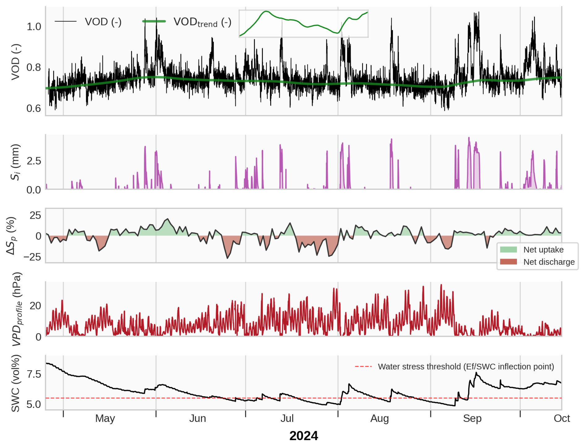
Figure 3Time series of GNSS-T vegetation optical depth (VOD), modeled interception storage (Si; modeled with CanWat), the plant water storage change (ΔSp; inferred from balancing sapflow and transpiration), vapor pressure deficit (VPD, measured along the canopy profile) and soil water content (SWC) for the growing season of 2024. The time series visualize the main drivers of VOD with Sp and Si, and provides insights into the responses of VOD to rainfall pulses and dry spells. The water stress threshold is determined by the inflection point of evaporative fraction (EF SWC), 5.5 vol %. The inlet at the top shows the VODtrend used in Eq. (5) to correct for seasonality in noise estimation.
To assess the actual storage, we integrate
where n is the current time step. Sp is a dimensionless, relative storage index. Because it is the running integral of a flux ratio (ΔSp, bounded at ±100 %) rather than of a physical flux, it is itself unbounded () and accumulates through several transformation steps. A single value of Sp therefore carries no direct physical meaning and should be interpreted qualitatively, through its temporal dynamics, rather than quantitatively.
We infer water limitation to the plants by determining the inflection point of the soil water content, SWCcrit, at which evaporation becomes limited by water accessibility. We use eddy-covariance based latent heat flux observations, and measurement of net radiation to calculate the evaporative fraction (), which is widely used as framework to detect water limitation (Lu et al., 2026; Seneviratne et al., 2010; Budyko, 1974). We found the ecosystem approaching SWCcrit at 5.5 vol % soil water content upon visual determination (Fig. S5). Note that the absolute values of soil water content are very low due to high fraction of gravel content at the site, however, this is not necessarily indicative for root zone water accessibility so that relative dynamics are still interpretable (Fig. 3).
2.6.2 Maximum-change framework
We test whether GNSS‐T VOD is sensitive to changes in plant water storage between saturation and maximum dehydration before substantial functional impairment of the tissues occurs, which we refer to as the maximum releasable plant water storage, . Then, we compare with the VOD noise threshold to test if GNSS-T VOD observations can – in theory – detect those changes, i.e. “maximum-change framework”. The empirical water-balance approach developed in the previous section cannot be used to constrain , because the study period did not contain sufficiently strong or long-lasting climatic extremes to reach drought conditions. As an alternative, we construct mechanistically from biomass data and hydraulic traits.
To define the upper and lower bounds of we use the concept of hydraulic equilibrium states, in which all plant compartments tend to approach a similar level of water potential (Binks et al., 2024, Fig. 1a, c). Such states are approached at night during periods of low flux (Donovan et al., 2003), and can occur under drought conditions when transpiration is strongly reduced. When stomata close, water fluxes approach zero (while residual conductance may continue at low rates) and the water potential can equilibrate throughout the plants (Mallick et al., 2016; Binks et al., 2024). The leaf turgor loss point (TLP) is a sensible indicator for this drought equilibrium state since TLP strongly related to stomatal conductivity, and onset of embolism formation (Brodribb et al., 2003).
Then, can be defined as the difference between the two hypothetical equilibrium states, at maximum in-vivo water saturation of the wood and leaves, and a lower limit at TLP. We parameterize the upper bound, , by maximum green (fresh) water content, θsat, individually for sapwood and leaves. For sapwood we use maximum green water content data from fresh samples and automated sawlog measurements (Ravoajanahary et al., 2025; Rosner et al., 2019), while leaf θsat is measured from a Picea abies forest with similar climatology, at Wetzstein (50°27′ N, 11°27′ E, 785 m a.s.l., Germany). The lower bound, , is the water storage at TLP. We derived by intersecting a linear water release curve with measured water potential at TLP Ψtlp. We use data of Ψtlp from pressure-volume curves for Picea abies at Tharandt. The slope of the function, the intensive hydraulic capacitance (Ci) is measured at Picea abies branches from sites across Europe. All trait ranges used in this study are summarized in Table 3 and the data source, and methodology is detailed in Appendix A4.
Table 3Hydraulic traits for Picea abies used for estimation of the maximum releasable water storage . Monte Carlo simulations with random trait combinations drawn from the reported ranges were used to propagate uncertainty.

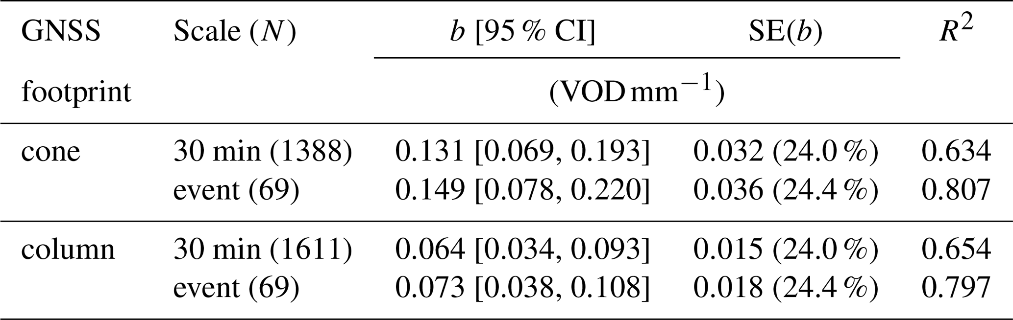
Table 4Regression results of VOD on interception storage Si at 30 min and event-scale aggregation for the season-wide fit of b for two spatial subsets: the inverted cone shape (the real GNSS look geometry), and a respective column (used for analysis per ground-area). The confidence interval (CI) and the standard error (SE) of b contain both, OLS sampling error with the propagated uncertainty of the CanWat model. The error margins for the OLS sampling error alone are shown given in Table S1; the coefficients for temporally variable b(t) in Table S2.
To translate these tissue-level traits into canopy-scale water storage, we scale water content with 3-D estimates of dry biomass from inventory and terrestrial laser scanning data, confined by the GNSS cone-shaped footprint. This follows the conceptual approach of scaling tissue water contents to ecosystem-level water storage proposed by Binks et al. (2024). For leaves and sapwood separately, ΔSp (mm) is
and are the plant water storage (mm) at saturation and turgor loss, respectively. AGB is the dry biomass of leaves or sapwood per ground area within the GNSS footprint (kg m−2); θsat and θtlp are intensive water content per dry biomass (gH2O g−1) in a maximum green/fresh state, and at turgor loss. We derive θtlp from linear water release curve whose slope is defined by Ci, the intensive hydraulic capacitance (), the tissue-specific θsat, and the turgor loss point Ψtlp by
where the second term indicates the constant saturation phase I between MPa (Hernando et al., 2025).
We derived the water-storing biomass in the GNSS-T footprint from using observations of plant area density (PAD, m2 m−3). PAD describes the combined leaf and wood area per volume air in a voxel is therefore indicative of all plant elements relevant to L-band transmission, in contrast, e.g., to leaf area index. Hereby, first, the plant density probability is calculated by counting the laser returns per 1 m3 voxels from terrestrial laser scans from a 2019 survey. To convert to a physical quantity, PAD is calibrated against radiation-based plant area index (Queck et al., 2012, 2014). The resulting canopy structure is shown in Figs. S1–S2. In the GNSS footprint the PAD distribution is highly left-skewed toward air voxels with a 0.05 m2 m−3 (mean), and tail 0.39 m2 m−3 (95th percentile); and higher at stand scale with 0.12 m2 m−3 (mean) and 0.83 m2 m−3 (95th percentile). The plant area index of the stand is 4.85 m2 m−2 (mean), with the tail of the distribution being 16.31 m2 m−2 (95th percentile). To ease the transfer of our approach to sites without 3-D structural data, we further report canopy-scale values for DE-Tha from the literature: The leaf area index was given as 7.6 for 1999 (Grünwald and Bernhofer, 2007), and the plant area index as 7.1 m2 m−2 (Queck et al., 2014), which agree well given the differences between the measurement methods. These values refer to measurements close to the tower, whereas the plant area index derived here is a spatial mean over the full scanned domain that includes canopy gaps and is therefore lower. We expect only minor changes at stand scale over time, since the overall stand structure has not changed fundamentally.
L-band has only limited penetration depth into living wood and measurements with dielectric probes suggest that wood deeper than about 5 cm contributes little to the total L-band emission (Koubaa et al., 2008; Mavrovic et al., 2018). Accordingly, much of the water stored in stems is likely not detectable by GNSS-T, and for this reason, we exclude heartwood and sapwood beyond 5 cm depth from the detectable storage pool. Still, all canopy constituents, all branch and leaves biomass are assumed conceptually to contribute to VOD because of their smaller size. We further neglect bark as a separate compartment by assuming hydraulic traits similar to the underlying sapwood, while acknowledging that bark may have distinct hydraulic properties in contrast to sapwood (Van Stan et al., 2021).
The uncertainty across trait methodologies and unaccounted spatial variability (e.g., canopy heterogeneity and vertical gradients) limit the robust estimation of ΔSp at the canopy scale. Therefore, we use a probabilistic approach and propagate uncertainty by Monte-Carlo sampling (20 000 draws/combinations), and report ΔSp as a probability distribution.
We estimate in the following steps (Summary of the workflow, see Fig. S6):
-
Estimate AGB for stems, branches and leaves using inventory data and allometric equations and restrict the hydraulically active tissue of the stem to 5 cm depth (Appendix A5, Fig. S7)
-
Create vertical distributions of AGB using terrestrial laser scans (Appendix A7)
-
Confine the 3-D to the canopy within the GNSS inverse-cone footprint (Appendix A8)
-
Estimate ΔSp using Monte-Carlo sampling of θsat, Ci, and Ψtlp for leaves and sapwood (Fig. S8)
We show alongside the maximum change of interception and dew, and . Hereby, is calculated as the maximum observed interception storage in the study period based on CanWat model output. is from the predicted nocturnally summed dew formation. However, due to VOD noise in the prediction (Eq. 11), we show the 95th percentile to account for outliers.
2.7 Accounting for biomass variability and seasonal Sp trends
Biomass variation is a strong driver in VOD (Ferrazzoli and Guerriero, 1996). In the mature, even-aged Norway spruce stand in Tharandt, however, it is reasonable to assume that stand-scale biomass varies only gradually with phenology or mortality, and biomass variation can be regarded negligible at short time scales. We study VOD in periods of canopy interception lasting at maximum 3 d, and along the diurnal cycle that we assume are biomass-constant. To account for biomass at those time scales, we normalize VOD, and likewise Sp to a pre-event reference time t0, defined over a window of length L preceding the event:
We denote normalized series with superscripts *noc or *dry for nocturnal or precipitation-free reference windows, respectively where VOD* and quantify change from the pre-event state. Note that VOD*(t) is derived from the normalized VOD time series of Sect. 2.2 and not from the noise decomposition of Eq. (5); the stationary diurnal Fourier series enters the definition of ϵ(t) only and is never imposed on the series that are compared with Sp, Si, or Sd. To provide a noise-robust VOD reference, we use the median in the reference window. Because Sp varies smoothly, the nighttime maximum is sufficient to represent near-equilibrium storage. For plant-water events we use a longer window (L=6 h) to maximize reference data, whereas for interception events a shorter window (L=2 h) retains enough data while still capturing chained interception events that fully dry between them. This way, we also correct for trends in canopy desiccation over the season which was out of focus of this study.
3.1 Rainfall interception
At the temperate needleleaf site Tharandt, we found VOD to strongly correlate with modeled interception storage Si (Fig. 4b), extending the evidence of recent GNSS-T studies showing sensitivity of VOD to interception storage and goes beyond correlations with precipitation as shown previously (Humphrey and Frankenberg, 2023; Schellenberg et al., 2024; Burns et al., 2025). While gross precipitation correlates with VOD, however, the relationship is noisier, owing to the interception process and retention that fall short in precipitation data (Fig. 4a and b). The intercepted storage could explain 63 % of the variance on VOD at 30 min resolution, with the slope b=0.131 VOD mm−1 (Table 4). The correlation increases at event-scale to 81 % of explained variance, and a slightly steeper slope of b=0.149 VOD mm−1. The confidence intervals of both slopes include the calibration uncertainty of the CanWat storage (Sect. 2.4), by which they are dominated; the same relationships carrying the OLS sampling error alone are shown in Fig. S13. Those results present confidence in the explanatory power of VOD to interception storage which increases with temporal aggregation from 30 min to full rain events.
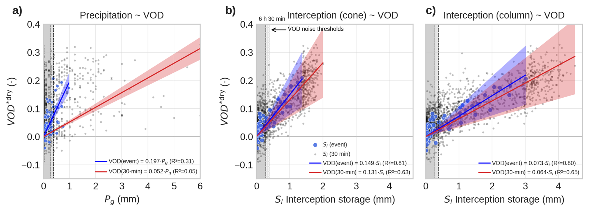
Figure 4Relationship between GNSS-T VOD with gross precipitation Pg as baseline (a), intercepted canopy water storage Si from the CanWat model for the GNSS footprint (b), and for an equivalent column footprint (c). Data is shown in 30 min (gray dots), and event-scale (blue dots) resolution across the entire season. The confidence interval (95 %) combining OLS sampling error and CanWat uncertainty propagation (for Pg: only OLS error) is shown as shaded ribbon around the regression line. The corresponding figures with the OLS error alone is given in Fig. S13.
The relationship with VOD is increasingly affected by scatter in the case of smaller precipitation inputs. At the 30 min scale, approximately 50 % of all the times when interception was present, the observation is affected by noise, i.e. Si is below δ30 min=0.38 mm (Table 1). This poses a limit of detectability to GNSS-T VOD for very small rain events. At event-scale, on average, 62.5 % of events are below the noise threshold, so detectability is limited for those events (δ6 h=0.28 mm, median length of rain event is 6 h). Note, however, that those events only account for 5.2 % of the total volume intercepted at Tharandt, thus, are mostly drizzle and the vast time that interception was present, it was detectable to the GNSS-T system.
We compared the influence of different footprint geometries, cone-shaped and column-shaped, on the correlation strength and found that correlations are equally high (Fig. 4c). This finding contradicts our hypothesis that the footprint bias would reduce the correlation strength between VOD and Si due to structural differences between the two footprint volume, e.g., in terms of water holding capacity. In absolute values, the influence of spatial domain is obvious. The b-slope in column is half the value of the cone, owing to the larger Si amounts in the columns.
Further, we observed that b varies across the season within a range of 0.112–0.137 VOD mm−1 (±10 % around the mean), with a minimum in May and a maximum in June, declining again towards autumn (Fig. 5, Table S2). Within the 95 % confidence intervals of the monthly fits, no clear seasonal signal can be resolved, since these intervals are dominated by the systematic calibration uncertainty of CanWat, which is independent of biomass variability itself. The OLS sampling error alone is considerably narrower (Fig. S14) and allows a clearer interpretation of the month-to-month contrasts. May carries the lowest slope and is separated from June, August, and September, whereas the months from June to September are indistinguishable from one another, and October falls between the two groups. This finding implies that b indeed contains a seasonal component that can be related to structural reorganization of the canopy with respect to its ability to intercept rain, e.g. the flush of new needles in spring and leaf aging towards fall.
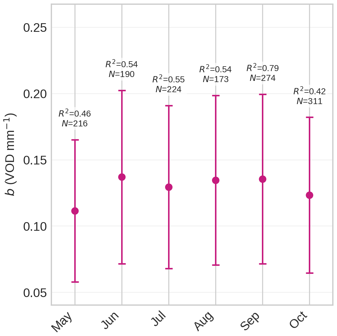
Figure 5Seasonal variability of the slope b(month) for the cone footprint geometry. The 95 % confidence interval combines the OLS sampling error of the slope with the calibration uncertainty of the CanWat storage. The corresponding interval without the CanWat term is shown in Fig. S14. The reader is referred to Table S2 for coefficients and statistical details.
On event scale, VOD sharply increases with interception across all precipitation event classes, highlighting the high sensitivity of the signal to rapid changes in canopy water balance (Fig. 6). This co-variation is consistent for light, moderate, and strong rainfall and scales with the intercepted water amount. During class III events, however, VOD exhibits a plateau during the rain phase-out, while modeled interception storage Si is already declining. This divergence suggests that additional water fluxes may confound the VOD–Si relationship.
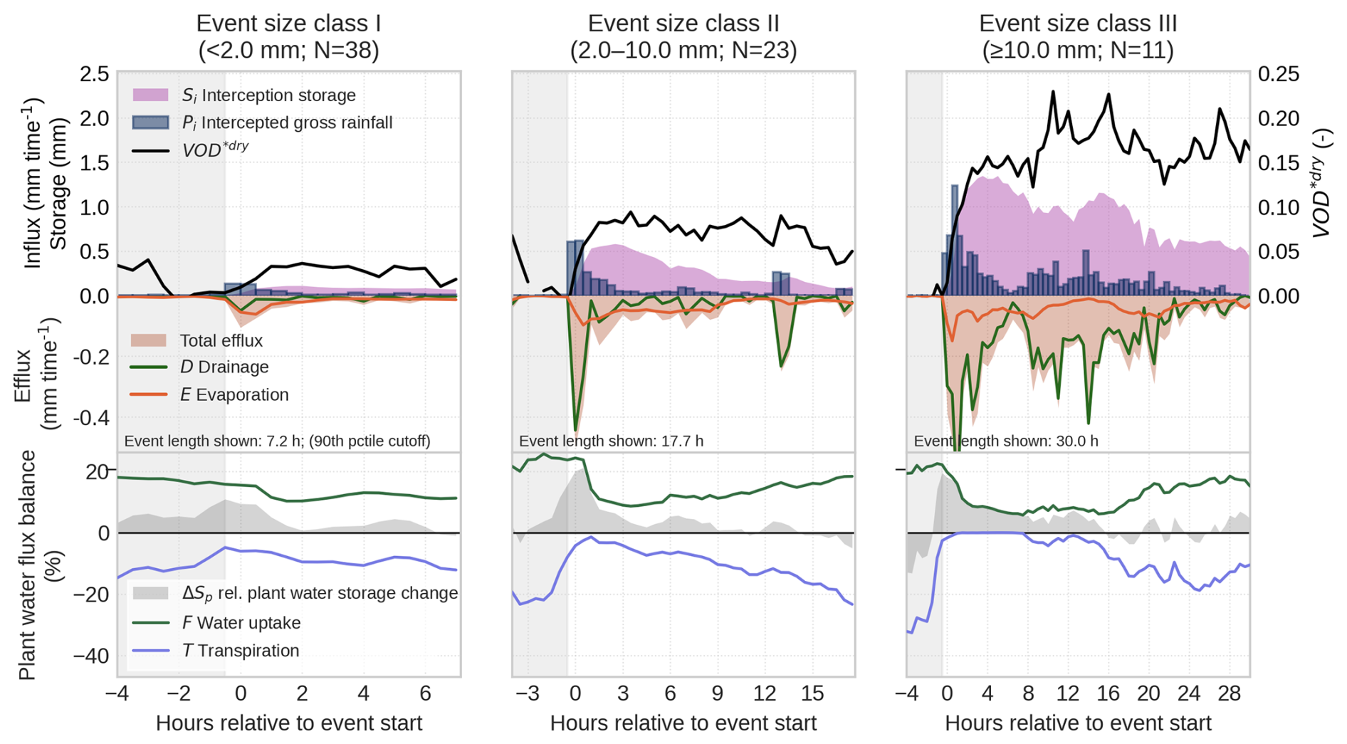
Figure 6Mean trajectory of precipitation events (N=72) grouped by rainfall intensity classes in the study period April–October 2024. Each class is shown up to the 90th percentile of its event length. Top and middle row: Influx (Pi) and effluxes (E and D) to the canopy interception storage Si; VOD is shown as normalized against 2 (dry canopy) hours before onset of precipitation. Bottom row: Plant water balance ΔSp as flux balance between plant water uptake F and transpiration T. All data shown is spatially confined to the GNSS footprint.
A likely confounder is plant water uptake during rainfall. Transpiration T is largely suppressed under wet-canopy conditions as CanWat closes the transpiration pathway when leaves are wet (Fig. 6, bottom panel). Also, water uptake F is also reduced after an initial peak shortly after rain onset, consistent with the physiological expectation that wet leaves and near-saturated vapor pressure deficits reduce stomatal conductance and thus sapflow (Ishibashi and Terashima, 1995). Even so, the net plant water flux balance ΔSp remains generally positive across all event classes, indicating continued net water influx into the trees during rainfall.
The extent to which this uptake alters plant water storage Sp strongly enough to affect VOD, however, remains uncertain. Because we lack absolute measurements of whole-canopy Sp, we cannot directly quantify its contribution to the signal. Instead, we use dry-canopy conditions, when interception is absent, to assess the co-variation between VOD and Sp over the diurnal cycle and use this relationship as a reference for wet-canopy periods (Fig. 7). Under dry conditions, VOD co-varies with Sp, but the relationship is associated with large statistical uncertainty. Moreover, plant storage changes during rainfall are 2.3 times smaller than under dry conditions, despite the clear rainfall-driven increase in VOD. Together, this suggests that water uptake during rain is substantial enough to contribute to the observed VOD plateau in prolonged events, but that its effect is likely secondary to the much stronger interception signal. We revisit the expected magnitude of Sp changes in the Tharandt spruce stand in more detail in Sect. 3.4.
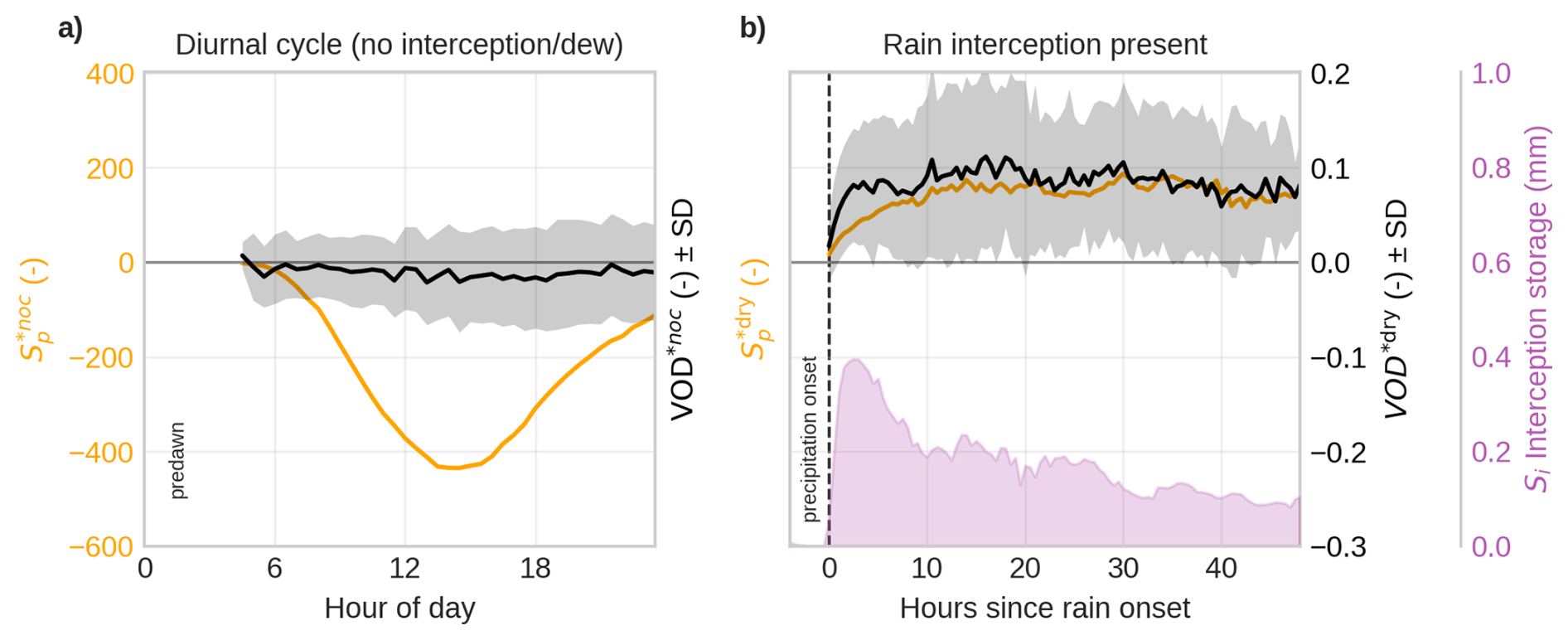
Figure 7Mean trajectory of VOD and plant water storage Sp, (a) for days diurnal cycles without interception, and (b) after onset of rain. VOD and Sp are normalized against a pre-event reference window to account for biomass. Dry canopy: nocturnal pre-dawn window of 6 h before sunrise (*noc); Wet canopy: 2 dry hours before onset of rain (*dry).
3.2 Dew formation
Dew formation on forest canopies can be a substantial water input and, simultaneously, adds an attenuating layer that affects VOD. Using hydrometeorological filters to estimate dew occurrence, we found that dew formed in 24.7 % of nights in the growing season. This is consistent with dew frequency reported for 19 forest ecosystems across the United States (25 ± 14 %, Ritter et al., 2019), and a temperate Douglas-fir forest in the North-Western US (28 %, Sibley et al., 2022), supporting the validity of this filtering approach. Of the forested sites in Ritter et al. (2019), five are evergreen needleleaf stands (RMNP, DEJU, JERC, TALL, OSBS) with a mean dew frequency of 24 %, although they cover a wide climatic range from montane and boreal to warm-humid conditions; the Douglas-fir stand of Sibley et al. (2022) is ecoclimatically the closest published analogue to Tharandt. Dew primarily formed during the climatologically transitional months of May and October, primarily around midnight (Fig. S9).
When comparing VOD at dew and non-dew events, we found a positive effect using a binary logistic regression (p<0.01). VOD values above 0.032 indicate the inflection point where dew conditions become more likely than non-dew. When VOD rises above 0.2, the probability of dew will exceed 80 % (Fig. 8a). In 67 % of all random dew/no-dew draws, VOD can distinguish between dew states, based on the area under the curve (AUC) classification performance metric. This shows that the conditions can be distinguished, but predictive power is limited. Note that the dew class is conservative by design (Sect. 2.5). The filters were set to minimize false positives at the cost of false negatives, so that part of the nocturnal reference is likely to contain undetected dew. The overlap of the two distributions in Fig. 8a is therefore expected.
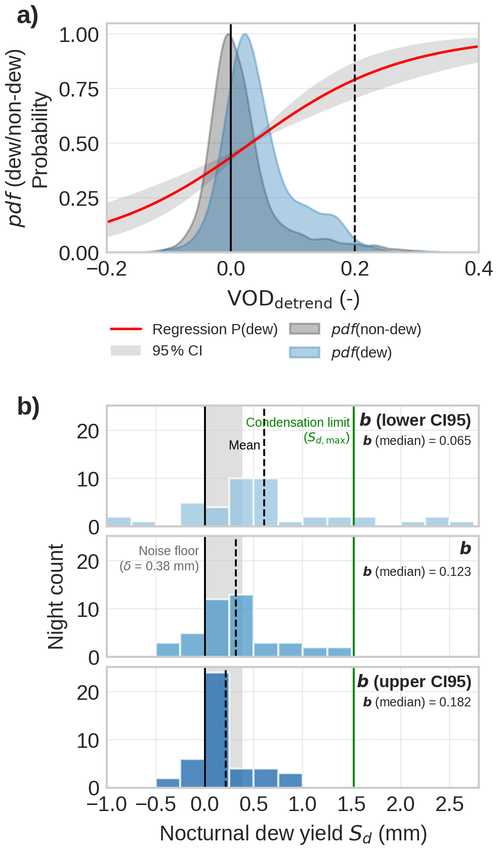
Figure 8Sensitivity of GNSS-T VOD to distinguish dew and non-dew conditions (a). The probability function P(dew)(red line) indicates the likelihood of dew detection for a given value of VOD. Dew yield prediction from VOD (b). The sub-panels show the yield obtained at the central estimate of b(month) and at the two ends of its 95 % confidence interval (Eq. 10); since the yield scales with , the lower confidence limit of b produces the higher yield. The shaded area represents the VOD noise floor at 30 min resolution. The mean yield is shown as a dashed vertical line. The corresponding prediction without the CanWat calibration term is shown in Fig. S15
We predict a mean dew formation of 0.32 (0.22–0.61) mm per night, and a 95th percentile of the nightly yields of 1.20 (0.81–2.29) mm per night (Fig. 8b), where the ranges give the 95 % confidence interval propagated from b(month); the same prediction without the CanWat error is shown in Fig. S15 to comply with the preprint version of this study. Firstly, we compare the dew predictions to reference measurements for forest ecosystems, which are usually about one magnitude smaller. Gerlein-Safdi et al. (2018) found a maximum of 0.051 mm per night for a savanna forest ecosystem from calibrated wetness sensors; Schneebeli et al. (2011) reports a maximum of 0.17 mm per night for a tropical canopy using microwave radiometers, similar to our approach. Reasons for this differences with our predictions can be manifold: difference in forest ecosystem, measurement method, failed timing of nights with larges dew formation, VOD noise; all of which hamper a fair comparison that can inform if dew amounts in this study are valid. Generally, there is a lack of data from forest ecosystems similar to our research site.
Secondly, as alternative to the scarce forest dew data, we test if dew predictions from VOD are biased high compared to maximum physically possible condensation. If all energy dissipated at night is used by condensation, the maximum dew formation reaches mm per night. The mean prediction of the 95th percentile remains below Sd,max and can therefore be regarded as physically plausible, whereas its upper confidence limit exceeds it. We read this overshoot as a constraint on the calibration rather than on the retrieval: because the yield scales with , values of b at the lower end of its confidence interval would imply dew amounts that are physically impossible, so that Sd,max in turn bounds how low b can plausibly be. The caveat of this approach is that Sd,max represents only a strict physical upper limit of dew formation. Due to competing sensible heat fluxes, heat storage, and atmospheric moisture constraints, as well as non black body-condition, actual dew is much lower, so the usefulness as upper boundary is limited to a strict physical limit.
Thirdly, as a more realistic upper boundary, artificial dew collections using material that facilitates condensation, have shown maximum dew formation of up to 0.6 mm per night (Tomaszkiewicz et al., 2015). While being less then half of the Sd,max, this values can be seen as a better real-world upper limit. Our mean prediction of 0.32 mm per night remains below this limit, but the upper end of the nightly distribution clearly exceeds it, which suggests an overestimation of the largest dew amounts by GNSS-T VOD. We attribute this overestimation primarily to residual VOD noise rather than to the conversion itself, as the same noise also produces the unphysical negative nightly yields seen in Fig. 8b. These negative values are retained rather than discarded, so that the mean yield remains unbiased. They are unlikely to represent evaporation of dew that the filter has missed, since no data after sunrise enter the nightly sums and vapor pressure deficit is typically lowest towards the end of the night.
3.3 Plant water dynamics
3.3.1 Plant-water coupling with VOD at seasonal and sub-daily scales
In this section, we assess the correlation of changes in plant water storage Sp and VOD at different time scales with respect to the influence of GNSS-T noise. On seasonal scale, when aggregating the diurnal cycles of GNSS-T VOD throughout the entire timeseries (excluding periods with surface water present), we found VOD to decline during the day, and increasing with night-time water replenishment (Fig. 7), consistent with literature (Holtzman et al., 2021; Humphrey and Frankenberg, 2023). However, the signal is associated with a large uncertainty band.
At shorter scales, the influence of noise is much stronger (Fig. 9). At 30 min intervals, VOD does not show a detectable association with Sp (R2=0). Even at days with water limitation, we found no association of Sp with VOD (Fig. 9a, orange dots). To suppress noise in VOD and to focus only on times of expected high water deficit, we aggregated the data to daily midday means (10:00–16:00 LT, Fig. 9b). However, likewise we could not find a detectable association (Fig. 9b, orange dots). Together, we could find a link between canopy hydration and VOD at the seasonal but not at the sub-daily scale, even when aggregating midday windows to reduce noise. Because the effect increased from diurnal to seasonal, it suggests that the water-content related information in VOD only become apparent after noise reduction by temporal aggregation. Using the computed noise thresholds (Table 1), we can assume that the canopy water storage did not change more than δ6 h>0.28 mm between pre-dawn and midday and hence, all variability in Sp stayed within the signal noise of VOD. This highlights the important role of signal noise and its effective mitigation to infer water status at diurnal scales.
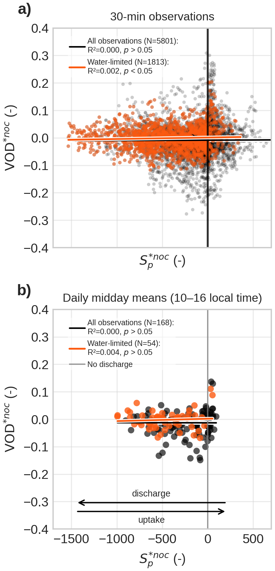
Figure 9Correlation of GNSS-T VOD to plant water storage (Sp) at sub-daily scales. (a) All 30 min observations from sunrise to midnight; (b) Daily values of midday means (10:00–16:00 LT). Highlighted in orange are water-limited days. Note that Sp is a dimensionless quantity and should only be interpreted relatively. It is the running integral of the flux ratio ΔSp, which equals +100 % when the plant water balance is entirely dominated by uptake and −100 % when it is entirely dominated by transpiration. VOD and Sp are normalized against a nocturnal pre-dawn reference window of 6 h before sunrise (*noc), so that each day starts at zero and both quantities are read as changes relative to that reference.
3.3.2 Maximum releasable water content in GNSS footprint
To explain this limited sub-daily detectability, we next assess the amount of plant water storage that is both visible to GNSS-T and hydraulically available for release within the measurement footprint.
First, the total amount of water stored in the canopy was estimated at 31.9 mm on column scale, of which 28.6 mm resided in woody compartments (branches and stem) and 3.25 mm in leaves. Because L-band penetration into living wood is limited, wood deeper than 5 cm was excluded from these calculations, so total tree water storage is higher than the microwave-visible fraction considered here.
Second, only a limited fraction of this biomass and associated water content falls within the GNSS measurement footprint. In the mature and structurally homogeneous Picea abies stand, we estimate that GNSS-T samples 16.3 % of the biomass and associated water visible at L-band relative to the column (Table 5). This fraction includes 14.1 % of stem sapwood and branches, but 35.6 % of leaves, indicating a pronounced bias of GNSS-T toward the upper canopy.
Third, when combining this footprint geometry with hydraulic traits that define saturation and threshold water contents, the maximum releasable plant water storage was only mm within the GNSS footprint, including 0.68 mm in wood and 0.20 mm in leaves. This is far smaller than the corresponding column-scale estimate of 4.82 mm, emphasizing that the GNSS system samples only a small and hydraulically constrained fraction of total canopy water storage.
Table 5Estimates for AGB and saturated plant water storage and maximum releasable plant water storage . The estimates differ between GNSS-T footprint (cone) and the equivalent column reference volume. “Tree” is the sum of sapwood and leaves.
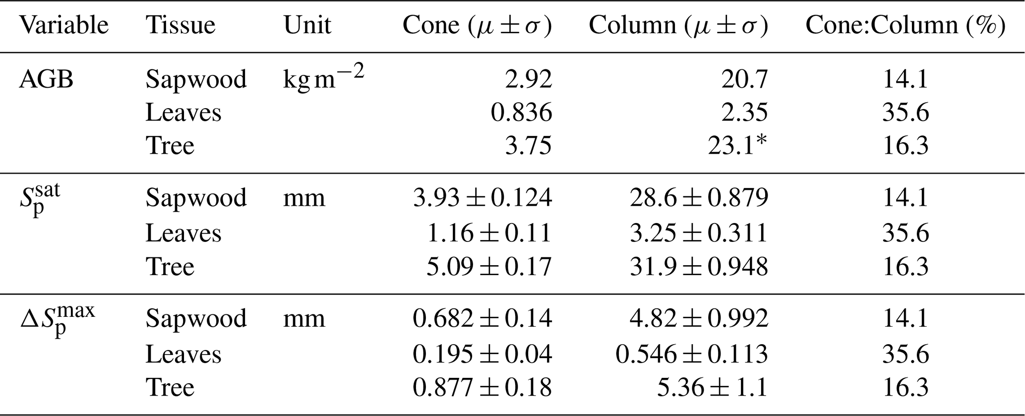
* cf. 21.3 kg m−2 from inventory in Grünwald and Bernhofer (2007), confirming validity of our estimate.
3.4 Signal-to-noise of water storage in VOD
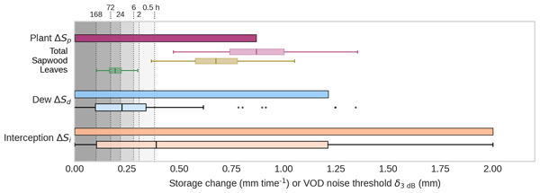
Lastly, we investigate the maximum expected volume of the water storages – interception, dew, and plant water – on the canopies in Tharandt in the growing season of 2024. Figure 10 provides a unified detectability comparison across the storage terms, relating them to the noise threshold. The comparison helps explain why interception is readily visible in VOD, whereas diurnal plant-water changes are not consistently detectable at short time scales.
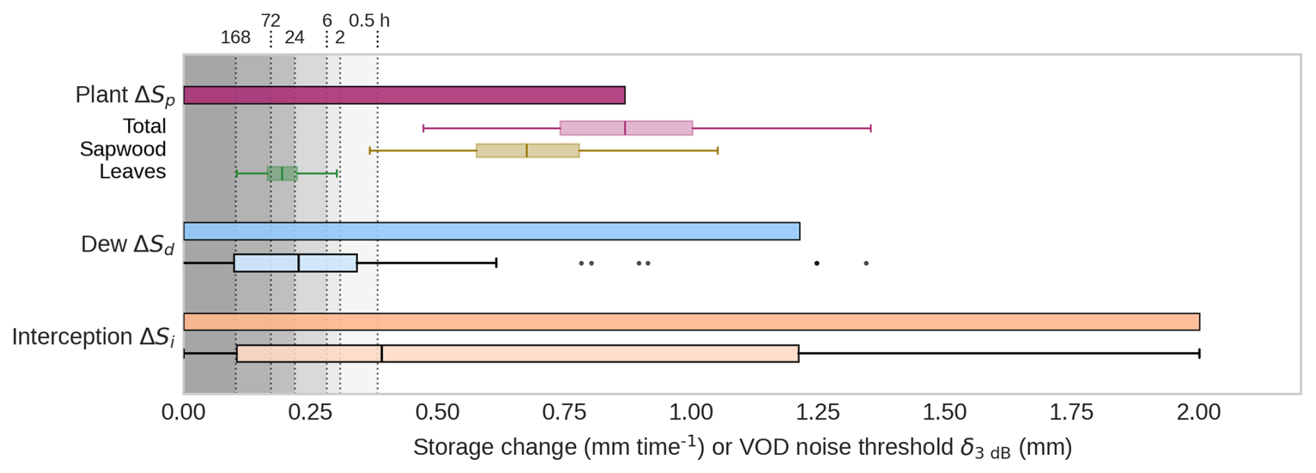
Figure 10Maximum expected changes of water storage terms in the GNSS footprint in comparison with VOD noise threshold δ3 dB at a range of typical temporal aggregation windows (shaded gray and dotted lines). Observations larger than the sensitivity thresholds δ3 dB can be interpreted as reasonably detectable by VOD. Plant water (top): Maximum releasable water storage , and for each tissue type, including uncertainty propagation from hydraulic traits. Dew (middle): Predicted dew formation per night at the 95th percentile (N=43), and the associated distribution across all nights with dew formation. Interception (bottom): Maximum modeled canopy interception from CanWat (N=1597), and the associated distribution of all 30 min intervals where interception was present.
In terms of surface water storages, interception ΔSi exceeds the noise threshold most frequently (Fig. 10, boxplot Si). For interception, about 50.3 % of 30 min instances exceed δ3dB, and detectability increases to 55.3 % when aggregating to 6 h event windows (Table 6). These results suggest that larger interception pulses can often be resolved already at sub-daily resolution. For small amounts of rain or for dew, the VOD should be aggregated over the event or nighttime, respectively.
Dew (ΔSd) is harder to detect at 30 min resolution, where only 23.3 % of cases exceed δ3dB. Detectability rises to 34.9 % when VOD is averaged to 6 h intervals (Table 6); this, however, requires dew to be present throughout the interval, which is an impractical constraint to the method, as the observed events last 2.9 h on average and rarely exceed 6 h (Fig. S17). Table 6 is therefore to be read as an if-then scenario that quantifies the sensitivity gained by noise reduction, and not as a matching of the averaging window to the observed event durations. The largest dew amounts, around 0.8 mm, are readily detectable (Fig. 10). We conclude that, because dew is a small flux, VOD needs further noise reduction, at best without lengthening the temporal interval, to detect most dew occurrences.
Finally, we found that is indeed larger than the VOD noise thresholds across all aggregation windows (30 min–7 d, Table 1). This implies that, in theory, the Tharandt spruce canopies can regularly lose water (until reaching TLP) so that change in plant water changes become visible in VOD. This, however, contrasts with the empirical observations shown in Fig. 9, where VOD did not respond detectably to plant water change under the daytime transpiration forcing. From this, we infer that the climatic drivers of dehydration (e.g., VPD, soil moisture) were likely not strong enough to trigger dry-down beyond δ despite occasional signs of water limitation. These results present the general mechanistic limits of detectability of plant water changes in change in VOD at the scope of a single site.
Table 6Surface water instances above VOD signal noise. Detectability is defined as signal exceeding the δ3 dB threshold. Interpretation: when VOD is aggregated to 6 h intervals, 55.3 % of interception instances and 34.9 % of dew instances exceed the detectability threshold of 0.28 mm.
4.1 Potential emerging method for monitoring whole-canopy interception
This study supports GNSS-T as a method for quantifying stand-scale rainfall interception in forest canopies that advances from wet/dry indication of rain-events (Schellenberg et al., 2024) to the direct estimation of the interception storage. Prior evidence from other VOD-based methods, including satellite radiometry (Xu et al., 2021), ground-based radiometry (Schneebeli et al., 2011), and within-canopy microwave transmissometry (Bouten et al., 1991) that all show sensitivity to interception, can now be similarly extended to GNSS-T.
The VOD noise threshold imposes a detectability limit that mainly affects drizzle and short rain events. Those events are the most frequent rainfall types, however, they account for only ∼ 5 % of total rainfall at Tharandt. Therefore, most of the rain can be sensed with GNSS-T VOD. Still, small inputs matter especially when moving from storage to the evaporation flux, another very important variable in the canopy water balance (Van Dijk et al., 2015). The smaller the rain inputs, the larger the fraction of evaporation to throughfall (see Fig. S10). Here, we provided an initial idea about the limits imposed by noise in the VOD signal to guide future evaporation analyses done with GNSS-T that.
The inferred VOD–Si slope, expressed by the attenuation parameter b, falls within the range of L-band values reported in the literature (Jackson and O'Neill, 1990; Van de Griend and Wigneron, 2004). Those values describe the relationship between VOD and the water held inside the vegetation while this study derived b from internal and surface water. Still the comparison is meaningful under the assumption of comparable attenuation by bound and free water introduced in Sect. 2.3. Within this limitation, it supports physical consistency with radiative-transfer expectations. The confidence interval of b is dominated by the systematic calibration error of CanWat (Sect. 2.4), which therefore sets the uncertainty band of every quantity that we convert from VOD into millimeters. Conclusions that rest on relative dynamics, such as the covariation of VOD with Si or the ranking of the storage terms against the noise floor, are insensitive to it, whereas the absolute amounts, i.e. the dew yield predictions carry it in full. The detectability threshold δ was deliberately converted with the season-wide b and without this term (Sect. 2.3), so that it remains one fixed reference across storage terms and aggregation windows. Still, b integrates structural properties of the canopy into an effective coefficient at GNSS footprint scale, and the monthly binning resolves only the coarsest part of its temporal variability. While the pre-event normalization used in this study reduces the direct effect of biomass changes that originate from seasonality, we found that the b coefficient describing the relationship between VOD and intercepted rain varies throughout season. This implies that fixed-b retrievals can introduce seasonal bias in inferred Si and b should be treated dynamically. Applications should therefore allow for site-specific and time-varying calibration of b, ideally linked to independent structural metrics such as LAI/PAI or leaf clumping. Multi-temporal lidar (Calders et al., 2023) or hemispheric photos (Brown et al., 2020) can help interpret b(t) dynamics and separate structural modulation from water-storage effects, and to track the effect of leaf orientation (Kattenborn et al., 2024).
A key limitation of our approach is that plant-water dynamics may interfere with the wetting signal, as shown in Fig. 7 and require isolation from rain inputs. In our case, we could show that water uptake was substantial, however given the low sensitivity to plant water variability on dry days, we can deduct only limited impact on the VOD-interception storage relationship. However, it can be argued that the confounding aspect of plants was non-zero. Future work should address this problem by explicitly accounting for water uptake in the VOD–Si relationship, e.g., by using direct observation of tree water status.
We found that the footprint choice (cone vs. column) matters for calibration and interpretation of absolute predicted storage, but not for correlation strength itself. This contradicts our hypothesis that geometric footprint matching would improve correlation strength. For structurally homogeneous stands (as in our case), this suggests that scaling from footprint to column is not a limitation, enabling direct prediction of interception storage per area ground using the b parameter fit for the column. However, this is unlikely to generalize to heterogeneous canopies or mixed stands with strong sub-footprint variability such as unequal changes in forest structure from species-specific phenological dynamics. Those cases will require explicit footprint-to-area scaling supported by independent structure data, such as lidar scans, which should be tested at more structurally complex sites.
4.2 Dew formation affects GNSS-T VOD
Dew occurred on about one quarter of nights and had a statistically significant but weak effect on GNSS-T VOD, indicating that canopy dew is detectable in principle but only with limited predictive skill. Although the VOD-derived dew amounts were physically plausible on average, the largest nightly predictions are higher than reported observations in literature, which suggests that GNSS-T overestimates dew at the upper end. As for interception, the dew amounts in millimeters inherit the calibration uncertainty of CanWat through b, so that their comparison with literature values and with the condensation limit is conditional on that calibration, while the separation of dew from dew-free nights is not.
A likely explanation is that the dew signal is small relative to residual VOD noise. Nocturnal aggregation windows were short, so substantial noise likely remained in the VOD data, and only 23.3 % of the dew state exceeded the 30 min detectability threshold (Table 6). Consistent with this, some very high VOD values in the dew class may have inflated the largest dew estimates (Fig. 8a). In addition, some events classified as dew may still have been affected by undocumented canopy wetness, including residual interception or fog. Such misclassification could arise from propagated errors in the CanWat model, for example if the canopy is classified as dry although it remains wet after rainfall. Resolving the origin of these large estimated dew events will require longer GNSS-T VOD time series and, ideally, independent observations of canopy dew and wetness.
Uncertainty also arises from the hydrometeorological filtering itself. The filters were intentionally conservative to avoid false positives in the dew class, but this likely caused some true dew events to be missed. Because these events remain in the nocturnal reference, they inflate its variability and thereby reduce the separation between the two classes; the discrimination reported in Sect. 3.2 is in this sense a conservative estimate. More generally, the filtering relies on meteorological variables measured within the canopy rather than at the leaf boundary layer where dew actually forms, so a mismatch between physical thresholds and the meteorological observation can become an issue. This problem is compounded by the general lack of reliable canopy-scale dew observations in forests (Ritter et al., 2019). Leaf-wetness sensors are highly local and may not represent the canopy as a whole (Binks et al., 2021), while leaf surface properties and hygroscopic structures can further modify the local microclimate and wetness state (Malik et al., 2014; Paulus et al., 2025). While such sensors were not available for our setup our reservation concerns their spatial representativeness across the canopy layers rather than the sensors as such so they would provide a valuable constraint on dew occurrence and amount in future deployments. Eddy-covariance measurements, in turn, are poorly constrained under the stable nocturnal conditions when dew forms (Paulus et al., 2022, 2024). At present, no single method can robustly detect and quantify dew formation at the scale of an entire forest canopy. Against this background, the sensitivity of GNSS-T VOD to dew is notable and deserves further attention as a promising complementary approach for observing canopy wetness.
4.3 VOD only weakly correlates with diurnal changes in plant water storage
In contrary to our initial hypothesis, diurnal changes in plant water storage were not directly detectable in GNSS-T VOD at sub-daily scales in Tharandt. This coupling only emerged after strong temporal aggregation, indicating that realized within-day plant water changes remained below the VOD noise floor during at sub-daily scales during the study period.
We interpret this weak diurnal coupling between VOD and plant water in Tharandt through a combination of drivers that jointly govern the hydraulic system. Firstly, the size of the system, i.e. the total water-retaining biomass, determines the storage capacity. The study site features a high-biomass forest (213 t ha−1), therefore a large storage capacity, i.e. we expect a large total water content. Secondly, the regulation of how readily water is released in response to atmospheric demand is influenced by stomatal regulation and hydraulic traits. Picea abies in Tharandt can be characterized as isohydric, i.e. with a conservative stomatal control that reduces transpiration at relatively high water potential under rising atmospheric demand (Leo et al., 2014; Paligi et al., 2024; Schumann et al., 2024). Hence, the expected realized relative water loss prior up until turgor loss is comparatively little, which however is counteracted with the large storage capacity. Thirdly, the climatic drivers determine whether the canopy is actually pushed towards this boundary of turgor loss. In this study, the ecosystem experienced the dry conditions, indicated by the lowest 25 % in terms of the local climatic water balance within the past 28 years (Fig. S11), and water limitation affected the trees throughout the dry-down (Fig. 3). Still, even during periods of water limitation, no variation in VOD at diurnal scales could be detected (Fig. 9). Finally, we infer that only a fraction of water loss was realized in the canopies that did not reach the maximum limit . Despite the large storage capacity and the partly water limiting conditions, plant water storage in Tharandt rarely exceeded the GNSS-T noise threshold at sub-daily and daily scales. A possible explanation are the conservative stomatal control if Picea abies. Operationally, diurnal plant-water dynamics are will become resolvable when changes in plant water storage exceed about ∼ 0.38 mm at 30 min resolution, corresponding to a VOD amplitude on the order of ∼ 0.05 (VOD), or lower when temporal aggregation mitigates noise.
The maximum-change framework also provides a coherent explanation for the contrasting results reported in GNSS-T studies. Specifically, while clear diurnal variations of VOD were present in a Mediterranean oak canopy (Humphrey and Frankenberg, 2023), this was not found in a subalpine spruce forest (Burns et al., 2025). The sites are similar in canopy height, which is indicative of biomass to a limited extent (Mediterranean: 5–15 m; Subalpine: 13–15 m). However, the tree species, differ in their hydraulic strategy: the Mediterranean species Quercus agrifolia is rather anisohydric ( MPa, Bartlett et al., 2012), while the subalpine species Picea engelmanii ( MPa, Lazarus et al., 2018, Fig. 7) is rather isohydric (conservative). Ultimately, the climatic conditions during the study periods also played a relevant role. While the Mediterranean site was hit by a strong heatwave with temperatures exceeding 40 °C during the study period (Humphrey and Frankenberg, 2023), the growing season was above-average wet at the subalpine site (Fig. S12). It remains unknown whether hydraulic traits or climatic forcing have ultimately induced the diurnal VOD variability in (Humphrey and Frankenberg, 2023). Nevertheless, the proposed framework provided a more directed view on the possible drivers under the light of strong noise in the GNSS-T VOD data.
Two assumptions underlie the empirical part of this comparison. Transpiration is taken from CanWat and was not validated independently at this site (Sect. 2.4), and the storage proxy Sp is a dimensionless index built on a seasonally closed flux balance, so that it is interpretable through its temporal dynamics rather than as an absolute storage (Sect. 2.6.1). Both restrict the comparison between VOD and Sp to relative changes, which is how we interpret it here.
A further important assumption in the maximum-change framework is that represents a conservative upper bound. Within the framework, we assume whole-canopy equilibration at the turgor loss point. This is, however, a hypothetical state that occurs before entering drought stress and is unlikely to be reached within diurnal timescales under non-drought conditions. Residual transpiration and within-canopy gradients maintain a water potential gradient, meaning realized canopy dry-downs are strictly smaller than . Uncertainty in arises from assumptions about static traits, biomass estimates and the prescribed L-band sensing depth. In future work, modeled or measured whole-canopy water content may be used to test the sensitivity of GNSS-T VOD to plant water variability directly. To attribute the VOD to water relation of the whole canopy, it there further necessary to understand the contributions of leaf and wood material to the signal, especially under the light of the maximum sensing depth.
This study evaluates whether GNSS-Transmissometry (GNSS-T) VOD can track short-term dynamics in forest canopy water storage and, in doing so, help bridge the gap between point-scale plant hydraulic measurements and stand-scale monitoring. By explicitly separating canopy water into interception (Si), dew (Sd), and internal plant water storage (Sp), we used the strong, pulse-like wetting signal of rainfall interception to calibrate the VOD-storage relationship and to translate the VOD noise floor into an equivalent detectability threshold for surface and internal water storage.
At the mature Picea abies stand in Tharandt, GNSS-T VOD robustly and approximately linearly tracked interception storage at 30 min and event scales during the growing season 2024, and instantaneous changes in Si provided a clearer predictor of VOD than precipitation alone. The inferred attenuation slope (b) was comparable in magnitude to values reported for L-band, which refer to internal vegetation water, but it varied across the season, implying that fixed-b approaches can introduce bias and that structure-aware, time-varying calibration is preferable. Using the calibrated relationship, we show that detectability is primarily constrained by measurement noise: at 30 min resolution, storage changes below about ∼ 0.38 mm (corresponding to a VOD amplitude of order ∼ 0.05 in this system) are frequently masked, while aggregation to longer time scales can reveal weaker signals by reducing noise. For dew, GNSS-T VOD produced plausible mean amounts, while the largest nightly predictions and the occasional negative estimates reflect residual noise that the short duration of dew events prevents from being averaged out.
We found only weak evidence that GNSS-T VOD captures diurnal variation in internal plant water status in Tharandt. The herein proposed detectability framework based on the maximum releasable canopy water storage provides a mechanistic interpretation for this finding: despite large potential storage capacity in this high-biomass forest, conservative hydraulic regulation and the actual climatic forcing during the study period likely kept realized water depletion well below the maximum possible and, crucially, below the GNSS-T noise threshold. Across these results, the qualitative conclusions rest on relative signal dynamics and are robust to the uncertainties of the underlying models, whereas the absolute water amounts and the detectability thresholds derived from them are conditional on the calibration of CanWat and on the transfer of b from internal to surface water.
To generalize beyond a single site-year, we propose using this maximum-change framework as a prospective tool for understanding GNSS-T site sensitivity to plant hydraulics. Unless the maximum realized water depletion in the GNSS footprint exceeds VOD noise at the temporal resolution of interest, the variability of forest water content will not be able to be resolved. Conversely, sites with higher effective biomass in the footprint, less conservative hydraulic regulation, or stronger atmospheric demand and sustained dry-down are more likely to yield detectable diurnal plant-water dynamics. Our framework allows for putting organ-specific biomass and hydraulic elasticity into context to understand the potential impact on VOD while proxies of the drivers themselves, i.e. the instantaneous canopy saturation Sp requires proxies.
Overall, GNSS-T emerges as a promising stand-scale method to quantify rainfall interception storage and, under favorable site and climate conditions (or with sufficient aggregation), to inform about surface wetness and plant water dynamics. We identify areas of potential progress in reducing both random and orbit-/geometry-related GNSS-T noise, transferring and stabilizing the effective attenuation coefficient b by linking it to independent canopy structure metrics across site. A deeper physical understanding of the interaction of the GNSS L-band radiation is equally important. Two pressing questions are: What fraction of stem cross-section is effectively contributing to the signal attenuation? and How does multi-path losses influence VOD and attenuation coefficient b at different biomass levels and incidence angles? Addressing these questions with extended acquisition scenarios, e.g., the multiple sensors at different heights and in space, and developing radiative transfer models tailored to the GNSS-T-geometry would help to isolate water pools in VOD. With these advances, emerging GNSS-T networks such as VODnet (Brede et al., 2025) can help doing this foundation work and validate satellite VOD products, and strengthen the monitoring of forest water content across ecosystems.
A1 Penmen-Rutter model: CanWat
The meteorological measurements used in the interception model CanWat can be found in Table A1.
Table A1Meteorological data used as climate forcing for CanWat, recorded at Tharandt station in 2024. Sensible heat flux only used for dew filters.
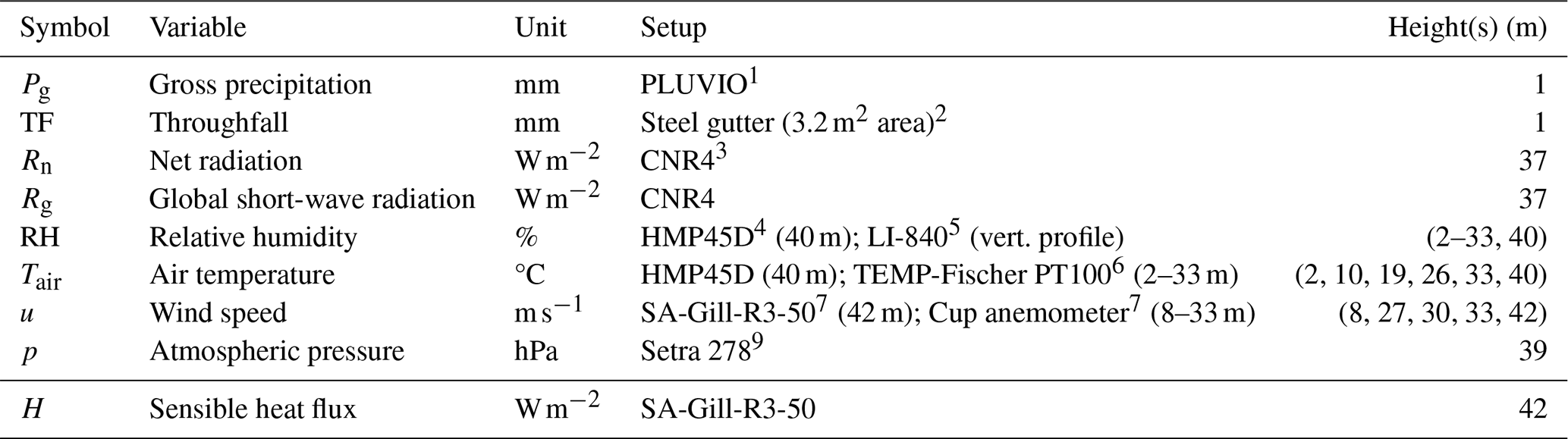
1 Measurement at nearby open field, Ott Messtechnik Gmbh & Co. KG, Kempten, Germany. 2 Water rinses to a barrel. Waters levels are then measured by a pressure sensor (Huba Control, Krefeld, Germany). 3 Kipp & Zonen, Delft, Netherlands. 4 Laborelektronik Ing. Peter Leskowa, Austria. 5 Integral of 12 vertical measurements. LI-COR Environmental, Lincoln, NE, United States. 6 Feingerätebau K. Fischer GmbH, Drebach, Germany. 7 Gill Instruments Ltd, Lamington, Hampshire, United Kingdom. 8 Adolf Thies GmbH &Co. KG, Göttingen, Germany. 9 Setra Systems, Boxborough, MA, United States.
A2 Per-satellite baseline normalization
The sparse and uneven hemispheric sampling of GNSS satellites over an inhomogeneous canopy imprints spurious patterns on the VOD time series. Humphrey and Frankenberg (2023) suppress it by normalizing every observation with the long-term mean VOD of the sky sector it falls into,
where φi and θi are the azimuth and the incidence angle of the sky sector, ti is the time of the observation, is the long-term mean of that sector and acts as the local biomass offset, and is a single scalar, the mean over the whole hemisphere, which restores the absolute level after the offset has been removed. In this manuscript, we amend this method by calculating the sky-sector mean separately for each satellite vehicle (SV),
so that the offset removed from an observation is the one of the satellite that produced it. Sky sectors are defined on the 1° hemispheric grid introduced in Sect. 2.2, and only observations with incidence angles below 60° contribute to the means. Since each satellite crosses a sector along its own track, it traverses a different part of the canopy volume and carries its own attenuation history; pooling all satellites into a single sector mean mixes these contributions and leaves more intensive periodic aliases in the time series. The effect of the modification, and of excluding the GLONASS constellation, is shown in Figs. S3–S4.
A3 Diurnal Fourier fit of the plant-water component
The third term of Eq. (5), VODplantwater(t), is a stationary diurnal Fourier series fitted to all dry-period days of the study period, i.e. after masking periods with dew or interception. We use a harmonic order of k=3, which keeps the model simple while allowing the mean diurnal cycle to depart from a single sine wave.
To verify that this order is adequate, we cross-validated the fit with a day-blocked scheme: the dry-period days were split into five random folds, the series was fitted on four fifths and used to predict the held-out fifth, and the procedure was repeated for harmonic orders k=0 to 6. The diurnal component explains a negligible fraction of the dry-period variance out of sample (R2≤0.24 %), and no meaningful improvement is obtained beyond k=3.
The consequence for Eq. (5) is that the term is practically negligible. The amplitude in the order of 0.01 VOD (Fig. S16c), roughly a factor of three below the residual scatter of ϵ(t) at 30 min resolution (Table 1), so that removing it would alter ϵ(t) only marginally. We nevertheless retain it to keep the decomposition physically interpretable, with the trend absorbing phenology and seasonal dry-downs and the diurnal term the sub-daily hydraulic variability, in line with Schellenberg et al. (2024). The small amplitude is itself consistent with our finding that VOD is not sensitive to diurnal changes in plant water at this site (Sect. 3.3). The full decomposition is shown in Fig. S16.
A4 Hydraulic traits
We use hydraulic traits of leaves and sapwood to estimate the maximum releasable water storage . In the following, we compare traits given by literature and own measurements to construct credible range for each trait that have been found for Picea abies:
-
Sapwood maximum green water content θsat (g g−1). We compile sapwood maximum green water content θsat from an automatically X-ray scanned sawlog dataset that reports a mean water content of g g−1 (Ravoajanahary et al., 2025). Kravka et al. (1999) report similar sapwood values, confirming the validity of the method. Hence, we use the upper standard bound of 1.42 g g−1 (mean + 1 SD) as a maximum estimate to infer θsat. Direct measurements of θsat report values of ≈1.27 g g−1 (Rosner et al., 2019). Finally, we combine these estimates by using a range of [1.27, 1.42] g g−1.
-
Leaf maximum water content θsat (g g−1). We sampled sunlit, top-canopy shoots (needles with supporting twigs from the current and previous two years) of adult Picea abies at Wetzstein, Germany (spruce monoculture; (Rebmann et al., 2010)) at predawn under wet conditions (10 July 2023, 05:00 LT; 8 samples from 4 trees). Fresh mass was recorded in the field; dry mass after 24 h oven-drying at 80 °C. We obtained leaf g g−1 (mean ± SD) which we use to build a Gaussian distribution.
-
Leaf turgor loss point Ψtlp (MPa). At Tharandt (4 July 2024) we sampled sunlit top-canopy branches (1–1.5 m) from three trees, transported in opaque bags, re-hydrated to full turgor overnight at 4 °C (tap water), and constructed PV curves following the “squeeze”-method (Sack et al., 2003) after verifying Ψ0<0.35 MPa. We obtained MPa. Comparable work reported values between −2 to −2.18 MPa (Paligi et al., 2024) using the same method.
-
Sapwood intensive hydraulic capacitance Ci (). 114 branches of Picea abies at 12 sites and 9 countries were sampled across a range of forest ecosystems in protected areas in Europe (Gene Conservations Units, part of EUFORGEN, de Vries et al., 2015) in fall of 2022. At each site 10 individuals were sampled in parallel transects with 30 m distance to each other. Two to three top canopy branches of lengths between 1.5–2.0 m were cut. After sampling the branches were recut under water, shipped to the laboratory, stored at 6 °C, and capacitance measurements carries out in less than a week from sample collection. The water release curve measurement started with weighing of the branch, and then stepwise desiccated by room temperature. Leaf water potential and weight was measured at each step after a period of 15–20 min in plastic bags to equalize the pressure in leaves and branch. We use capacitance of phase II (elastic phase) which features the longest, linear section of the water release curve. Therefore, the release curve initiates at the inflection point between phase I and II (−0.2 MPa). For more details on the method and release curve construction, the reader is referred to Hernando et al. (2025). The mean value of Ci is 0.12 ± 0.03 across all branches and sites. We chose all sites in order to increase confidence in the statistic and receive a species-agnostic value.
A5 Allometry and hydraulically activate plant compartments
We use inventory data of 126 Picea abies individuals acquired over an area of 2500 m2 around the eddy covariance tower in 2024. The stand consists of trees that are planted in 1887 (138 years at time of writing). A small number of Larix decidua individuals (N=6) are present which we excluded from our analysis. The GNSS footprint is in close proximity to the inventory plots, however, does not directly overlap. Still, we can assume that tree properties between the inventory plot and the GNSS footprint are similar due to the species and age homogeneity in the Picea abies monoculture.
We use log-log allometric functions to estimate per-tree AGB for stems, branches and leaves based on the inventory properties diameter at breast height (DBH), tree height (h), and age (see Table A3). The equations are with high accuracy (R2>90 %) defined based on a meta-dataset of 688 trees in 102 stands covering Central Europe and explain AGB variances of > 90 % (Wirth et al., 2004):
where the subscripts st, br and lf denote stem, branch and leaf components, respectively. The coefficients βi, the standard deviation σ, and the goodness-of-fit (R2) of the regression are given in Table A2 (Wirth et al., 2004).
Table A2Fitted allometric parameters for stem, branches, and foliage from Wirth et al. (2004) estimate AGB of tree components based on DBH, canopy height, and age.

Table A3Properties of inventory trees (N=132) that are use in the allometric equations.
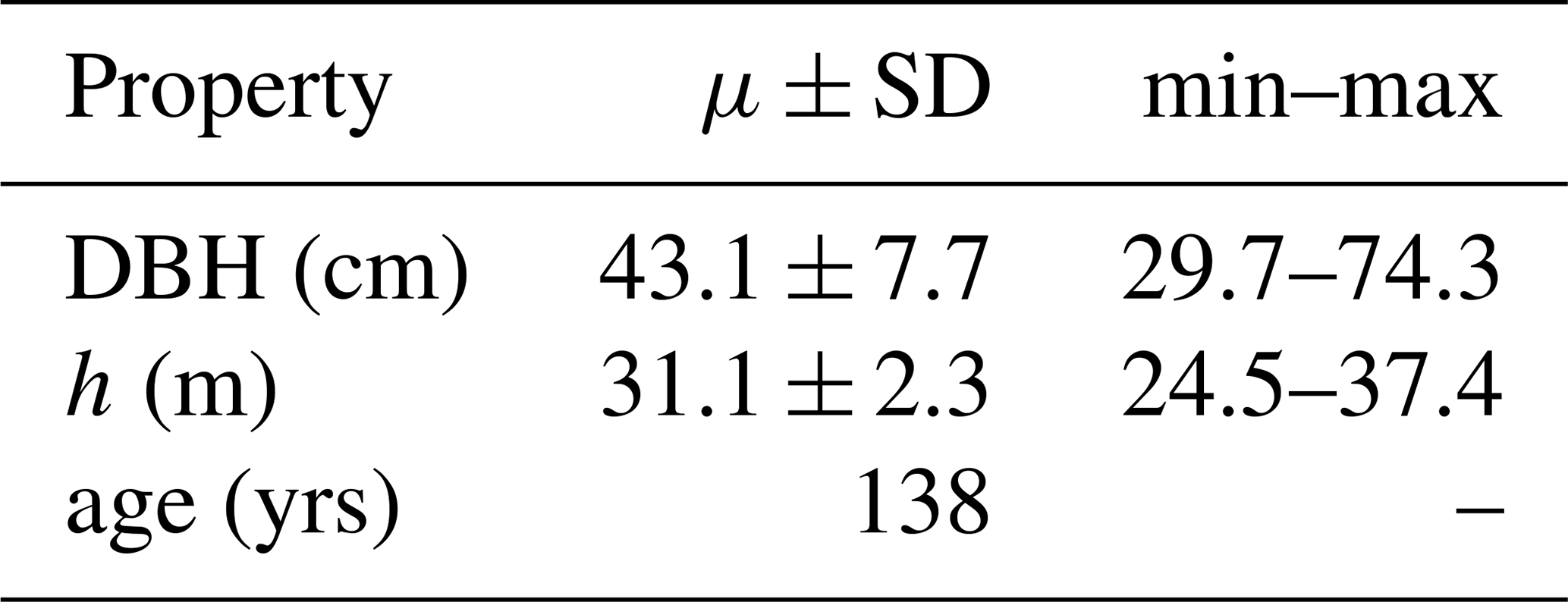
A6 Visible stem fraction
The fraction of stem sapwood detectable to the GNSS signal is determined by
where rinvis is the L-band-invisible stem diameter (m) V is the function for cone volumes (m3), values for the radii are used from literature (see Table A4). A similar approach can be found in (Kravka et al., 1999).
Table A4Definitions of variables used to calculate the fractional AGB of sapwood in the stem.
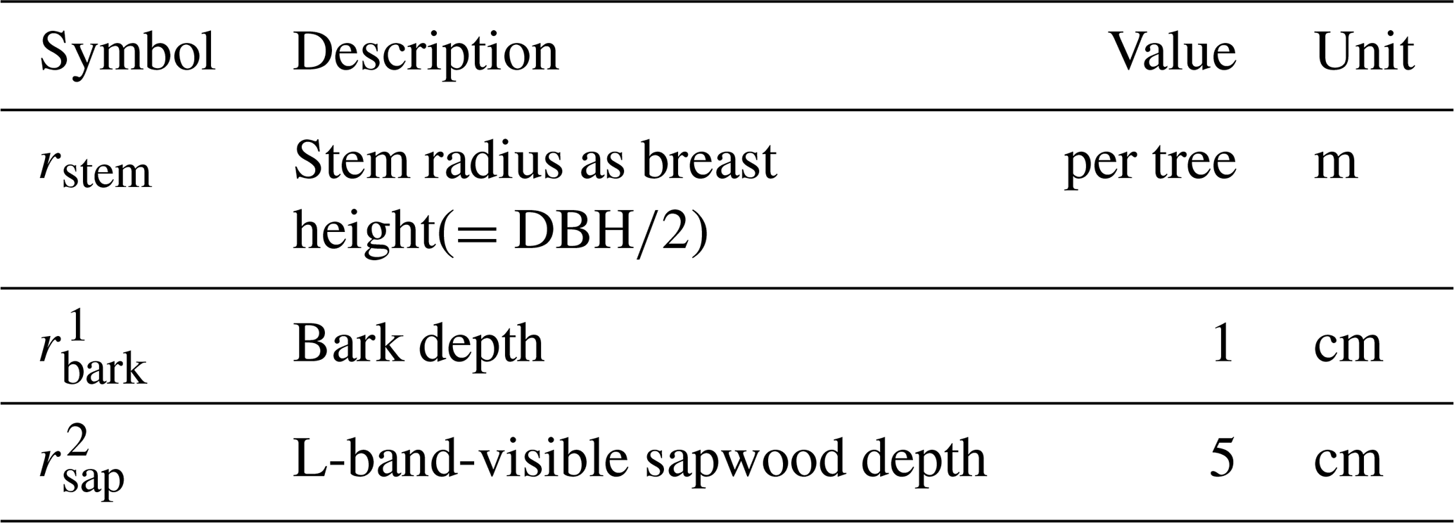
1 Estimated from an extensive dataset of 7712 Picea abies trees (Altherr et al., 1978), 2 Assuming only 5 cm L-band visibility into the sapwood according to (Koubaa et al., 2008).
Finally, we estimate tree, branch and leaf biomass per ground area by normalizing each quantity with the ground area (2500 m2), see Table A5.
Table A5Inventory data and AGB for specific plant compartment across the plot (2500 m2 total ground area).
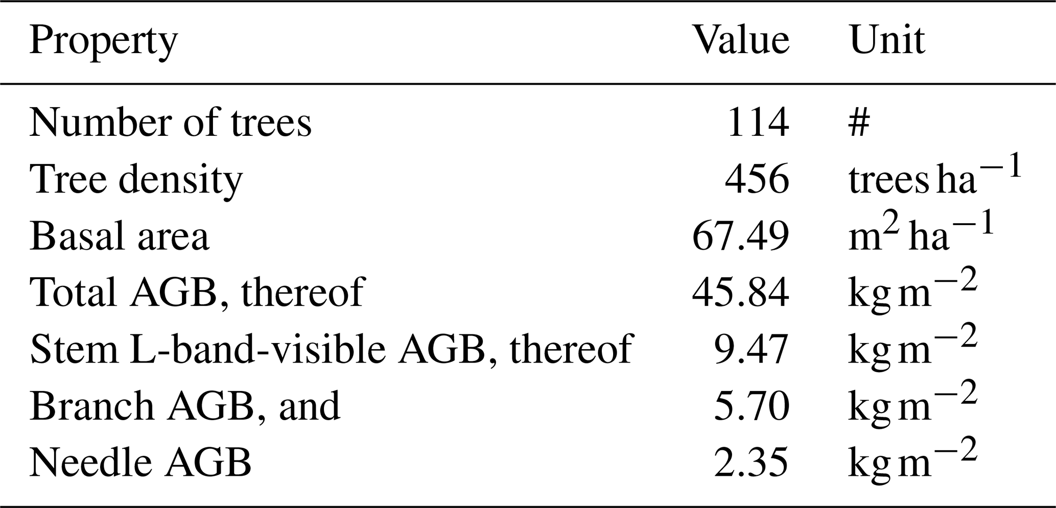
A7 Vertical distribution
To estimate the AGB in this GNSS footprint, it is required to convert ground area-based AGB to a cone-volume basis using a height model. For this purpose, we use terrestrial laser scanning (TLS)-derived plant area density which captures the vertical leaf and branch distribution. However, TLS-based plant area density (PAD) contains any vegetation material, including stems. We disentangle the crown distribution (leaves and branches) from stems by first calculating the stem volume using PAD (m2 m−2) at heights 2–5 m, assuming purely stem contributions, yielding PADstem(z); then, extrapolating this volume to canopy height assuming linear tapering of the stems to the top. Then, the crown probability density function (pdf) is calculated by
where z denotes the height slice in meters and dz is the step-length in height (here: 1 m). The pdf of the L-band-visible stem is then calculated by using the geometrical cone function:
Now, the height-weighted AGB contributions for sapwood and leaf can be calculate for each canopy compartment by
The hydraulically active plant biomass is ; and its vertical distribution is shown in Fig. S7a.
A8 GNSS footprint
The intersection of the GNSS footprint with stand biomass is the part of the canopy seen by the GNSS. First, the probability for a height slice to fall into the GNSS cone footprint is given by
where θ is the incidence angle (from nadir) and h is the maximum canopy height (Fig. S7c). Then, the total AGB falling into the GNSS footprint is given by
and shown in Fig. S7b.
The code to perform the formal analysis and to generate the figures is available on GitHub (https://github.com/konstantinschellenberg/eval-gnsst-vod-forest-water-content, last access: 19 November 2026; https://doi.org/10.5281/zenodo.24318671, Schellenberg, 2026).
The associated data set of pre-processes GNSS, meteorological data, outputs from CanWat is accessible on Zenodo (https://doi.org/10.5281/zenodo.19356983, Schellenberg et al., 2026).
The interception model CanWat is published on GitHub (https://github.com/Ron-Q/CanWat, last access: 19 November 2026).
The supplement related to this article is available online at https://doi.org/10.5194/bg-23-8507-2026-supplement.
TJ, SP, RQ, and KS planned and designed the study. MM, OB, and SP provided supporting data and expertise. KS carried out the measurements, analyzed the data, and prepared the original draft under the supervision of TJ, HH, and CS. All authors discussed, reviewed, and edited the paper.
The contact author has declared that none of the authors has any competing interests.
Publisher's note: Copernicus Publications remains neutral with regard to jurisdictional claims made in the text, published maps, institutional affiliations, or any other geographical representation in this paper. The authors bear the ultimate responsibility for providing appropriate place names. Views expressed in the text are those of the authors and do not necessarily reflect the views of the publisher.
The authors would like to thank Jianbei Huang for financial support for the GNSS setup at Tharandt; Matthias Mauder, Thomas Grünwald and Markus Hehn for providing meteorological and inventory data from the station DE-Tha and helping with the GNSS setup; the Bayerische Landesanstalt für Wald und Forstwirtschaft for providing sapflow data. Finally, we would like to thank two anonymous reviewers for their helpful and constructive feedback on this manuscript. During the preparation of this work, the authors used ChatGPT- 5.3 (OpenAI) for language refinement. All material was subsequently reviewed and revised by the authors, who take full responsibility for the manuscript’s final version.
KS was supported by funding through the International Max Planck Research School for Global Biogeochemical Cycles (IMPRS-gBGC). Further, MM would like to acknowledge support by EU‐H2020 programme via grant 862221 FORGENIUS (Improving access to FORest GENetic resources Information and services for end-USers). SJP would like to acknowledge support by EU‐Horizon Europe programme via grant 101184989 – NextGenCarbon (Next Generation Modelling of Terrestrial Carbon Cycle by assimilation of in-situ campaigns and Earth Observations). DC as been funded by the projects “la Caixa” Junior Leader Fellowship LCF/BQ/PI25/12100008 (lead: DC) and LCF/BQ/PI23/11970013 (lead: OB) and by the project FORGENIUS. SSP acknowledges financial support received from the German Research Foundation (DFG) through the Research Training Group 2300 (316045089/GRK2300). TJ is supported by the DFG-514721519 in the project “Remote sensing of vegetation canopy properties: States and spatiotemporal dynamics” as part of the DFG Research Unit 5639: Land Atmosphere Feedback Initiative (LAFI).
The article processing charges for this open-access publication were covered by the Max Planck Society.
This paper was edited by Andreas Ibrom and reviewed by two anonymous referees.
Altherr, E., Unfried, P., Hradetzky, J., and Hradetzky, V.: Statistische Rindenbeziehungen als Hilfsmittel zur Ausformung und Aufmessung unentrindeten Stammholzes: Teil IV: Fichte, Tanne, Douglasie und Sitka-Fichte, Forstliche Versuchs- und Forschungsanstalt Baden-Württemberg, Freiburg im Breisgau, 90, 1978. a
Arend, M., Link, R. M., Patthey, R., Hoch, G., Schuldt, B., and Kahmen, A.: Rapid hydraulic collapse as cause of drought-induced mortality in conifers, P. Natl. Acad. Sci. USA, 118, e2025251118, https://doi.org/10.1073/pnas.2025251118, 2021. a
Bartlett, M. K., Scoffoni, C., and Sack, L.: The determinants of leaf turgor loss point and prediction of drought tolerance of species and biomes: a global meta‐analysis, Ecol. Lett., 15, 393–405, https://doi.org/10.1111/j.1461-0248.2012.01751.x, 2012. a, b
Beysens, D.: Dew nucleation and growth, C. R. Phys., 7, 1082–1100, https://doi.org/10.1016/j.crhy.2006.10.020, 2006. a
Binks, O., Finnigan, J., Coughlin, I., Disney, M., Calders, K., Burt, A., Vicari, M. B., Da Costa, A. L., Mencuccini, M., and Meir, P.: Canopy wetness in the Eastern Amazon, Agr. Forest Meteorol., 297, 108250, https://doi.org/10.1016/j.agrformet.2020.108250, 2021. a
Binks, O., Meir, P., Konings, A. G., Cernusak, L., Christoffersen, B. O., Anderegg, W. R. L., Wood, J., Sack, L., Martinez-Vilalta, J., and Mencuccini, M.: A Theoretical Framework to Quantify Ecosystem Pressure-Volume Relationships, Glob. Change Biol., 30, e17567, https://doi.org/10.1111/gcb.17567, 2024. a, b, c, d
Bouten, W., Swart, P. J. F., and De Water, E.: Microwave transmission, a new tool in forest hydrological research, J. Hydrol., 124, 119–130, https://doi.org/10.1016/0022-1694(91)90009-7, 1991. a
Brede, B., Schellenberg, K., Camps, A., Chaparro, D., Damm, A., Forkel, M., Frankenberg, C., Abesh Ghosh, Hartmann, H., Herold, M., Humphrey, V., Jagdhuber, T., Konings, A., Kurum, M., Niederberger, M., Schmullius, C., Stassin, T., Steele-Dunne, S., Van Der Borght, N., Strube, M., Vermunt, P., Yitong Yao, Monteith, A., Richards, E., Persson, H., Lecart, B., and Jonard, F.: VODnet: a virtual GNSS-T VOD network for monitoring of forest water budget and structure, ResearchGate, https://doi.org/10.13140/RG.2.2.17146.35522, 2025. a
Brodribb, T. J. and McAdam, S. A.: Evolution of the Stomatal Regulation of Plant Water Content, Plant Physiol., 174, 639–649, https://doi.org/10.1104/pp.17.00078, 2017. a
Brodribb, T. J., Holbrook, N. M., Edwards, E. J., and Gutiérrez, M. V.: Relations between stomatal closure, leaf turgor and xylem vulnerability in eight tropical dry forest trees, Plant Cell Environ., 26, 443–450, https://doi.org/10.1046/j.1365-3040.2003.00975.x, 2003. a
Brown, L. A., Ogutu, B. O., and Dash, J.: Tracking forest biophysical properties with automated digital repeat photography: A fisheye perspective using digital hemispherical photography from below the canopy, Agr. Forest Meteorol., 287, 107944, https://doi.org/10.1016/j.agrformet.2020.107944, 2020. a
Budyko, M. I.: Climate and Life, Academic Press, ISBN 978-0-12-139450-9, 1974. a
Burns, S. P., Humphrey, V., Gutmann, E. D., Raleigh, M. S., Bowling, D. R., and Blanken, P. D.: Using GNSS-based vegetation optical depth, tree sway motion, and eddy covariance to examine evaporation of canopy-intercepted rainfall in a subalpine forest, Biogeosciences, 22, 5741–5769, https://doi.org/10.5194/bg-22-5741-2025, 2025. a, b, c, d
Calders, K., Brede, B., Newnham, G., Culvenor, D., Armston, J., Bartholomeus, H., Griebel, A., Hayward, J., Junttila, S., Lau, A., Levick, S., Morrone, R., Origo, N., Pfeifer, M., Verbesselt, J., and Herold, M.: StrucNet: a global network for automated vegetation structure monitoring, Remote Sensing in Ecology and Conservation, 9, 587–598, https://doi.org/10.1002/rse2.333, 2023. a
Camps, A., Alonso-Arroyo, A., Park, H., Onrubia, R., Pascual, D., and Querol, J.: L-Band Vegetation Optical Depth Estimation Using Transmitted GNSS Signals: Application to GNSS-Reflectometry and Positioning, Remote Sensing, 12, 2352, https://doi.org/10.3390/rs12152352, 2020. a
Chaparro, D., Jagdhuber, T., Piles, M., Jonard, F., Fluhrer, A., Vall-llossera, M., Camps, A., López-Martínez, C., Fernández-Morán, R., Baur, M., Feldman, A. F., Fink, A., and Entekhabi, D.: Vegetation moisture estimation in the Western United States using radiometer-radar-lidar synergy, Remote Sens. Environ., 303, 113993, https://doi.org/10.1016/j.rse.2024.113993, 2024. a
Cisneros Vaca, C., van der Tol, C., and Ghimire, C. P.: The influence of long-term changes in canopy structure on rainfall interception loss: a case study in Speulderbos, the Netherlands, Hydrol. Earth Syst. Sci., 22, 3701–3719, https://doi.org/10.5194/hess-22-3701-2018, 2018. a
de Vries, S. M., Alan, M., Bozzano, M., Burianek, V., Collin, E., Cottrell, J., Ivankovic, M., Kelleher, C. T., Koskela, J., Rotach, P., and Vietto, L.: Pan‐European Strategy for Genetic Conservation of Forest Trees and Establishment of a Core Network of Dynamic Conservation Units., vol. 40 of European Forest Genetic Resources Programme (EUFORGEN), Bioversity International, Rome, Italy, https://www.euforgen.org/fileadmin/templates/euforgen.org/upload/Publications/Thematic_publications/EUFORGEN_FGR_conservation_strategy.pdf (last access: 17 November 2026), 2015. a
Donovan, L. A., Richards, J. H., and Linton, M. J.: Magnitude and Mechanisms of Disequilibrium Between Predawn Plant and Soil Water Potentials, Ecology, 84, 463–470, https://doi.org/10.1890/0012-9658(2003)084[0463:MAMODB]2.0.CO;2, 2003. a
Dorigo, W., Dietrich, S., Aires, F., Brocca, L., Carter, S., Cretaux, J.-F., Dunkerley, D., Enomoto, H., Forsberg, R., Güntner, A., Hegglin, M. I., Hollmann, R., Hurst, D. F., Johannessen, J. A., Kummerow, C., Lee, T., Luojus, K., Looser, U., Miralles, D. G., Pellet, V., Recknagel, T., Vargas, C. R., Schneider, U., Schoeneich, P., Schröder, M., Tapper, N., Vuglinsky, V., Wagner, W., Yu, L., Zappa, L., Zemp, M., and Aich, V.: Closing the Water Cycle from Observations across Scales: Where Do We Stand?, B. Am. Meteorol. Soc., 102, E1897–E1935, https://doi.org/10.1175/BAMS-D-19-0316.1, 2021. a
Dzikiti, S., Steppe, K., Lemeur, R., and Milford, J.: Whole-tree level water balance and its implications on stomatal oscillations in orange trees [Citrus sinensis (L.) Osbeck] under natural climatic conditions, J. Exp. Bot., 58, 1893–1901, https://doi.org/10.1093/jxb/erm023, 2007. a
Feldman, A. F.: Emerging Methods to Validate Remotely Sensed Vegetation Water Content, Geophys. Res. Lett., 51, e2024GL110505, https://doi.org/10.1029/2024GL110505, 2024. a
Ferrazzoli, P. and Guerriero, L.: Passive microwave remote sensing of forests: a model investigation, IEEE T. Geosci. Remote, 34, 433–443, https://doi.org/10.1109/36.485121, 1996. a
Fischer, S., Moderow, U., Queck, R., and Bernhofer, C.: Evaporation of intercepted rainfall – Comparing canopy water budget and energy balance related long term measurements at a Norway spruce site, Agr. Forest Meteorol., 341, 109637, https://doi.org/10.1016/j.agrformet.2023.109637, 2023. a
Fischer, S., Queck, R., Bernhofer, C., and Mauder, M.: Quantifying evaporation of intercepted rainfall: a hybrid correction approach for eddy-covariance measurements, Hydrol. Earth Syst. Sci., 30, 965–984, https://doi.org/10.5194/hess-30-965-2026, 2026. a, b
Frappart, F., Wigneron, J.-P., Li, X., Liu, X., Al-Yaari, A., Fan, L., Wang, M., Moisy, C., Le Masson, E., Aoulad Lafkih, Z., Vallé, C., Ygorra, B., and Baghdadi, N.: Global Monitoring of the Vegetation Dynamics from the Vegetation Optical Depth (VOD): A Review, Remote Sensing, 12, 2915, https://doi.org/10.3390/rs12182915, 2020. a
Gerlein-Safdi, C., Koohafkan, M. C., Chung, M., Rockwell, F. E., Thompson, S., and Caylor, K. K.: Dew deposition suppresses transpiration and carbon uptake in leaves, Agr. Forest Meteorol., 259, 305–316, https://doi.org/10.1016/j.agrformet.2018.05.015, 2018. a
Green, S., Clothier, B., and Jardine, B.: Theory and Practical Application of Heat Pulse to Measure Sap Flow, Agron. J., 95, 1371–1379, https://doi.org/10.2134/agronj2003.1371, 2003. a
Grunicke, S., Queck, R., and Bernhofer, C.: Long-term investigation of forest canopy rainfall interception for a spruce stand, Agr. Forest Meteorol., 292–293, 108125, https://doi.org/10.1016/j.agrformet.2020.108125, 2020. a, b, c, d
Grünwald, T. and Bernhofer, C.: A decade of carbon, water and energy flux measurements of an old spruce forest at the Anchor Station Tharandt, Tellus B, 59, 387, https://doi.org/10.1111/j.1600-0889.2007.00259.x, 2007. a, b, c
Grünwald, T., Wanner, L., Eichelmann, U., Hehn, M., Moderow, U., Prasse, H., Queck, R., Bernhofer, C., and Mauder, M.: Carbon fluxes controlled by land management and disturbances at a cluster of long-term ecosystem monitoring sites in Central Europe, Agr. Forest Meteorol., 369, 110533, https://doi.org/10.1016/j.agrformet.2025.110533, 2025. a
Guerriero, L., Martín, F., Mollfulleda, A., Paloscia, S., Pierdicca, N., Santi, E., and Floury, N.: Ground-Based Remote Sensing of Forests Exploiting GNSS Signals, IEEE T. Geosci. Remote, 58, 6844–6860, https://doi.org/10.1109/TGRS.2020.2976899, 2020. a
Hammond, W. M., Williams, A. P., Abatzoglou, J. T., Adams, H. D., Klein, T., López, R., Sáenz-Romero, C., Hartmann, H., Breshears, D. D., and Allen, C. D.: Global field observations of tree die-off reveal hotter-drought fingerprint for Earth's forests, Nat. Commun., 13, 1761, https://doi.org/10.1038/s41467-022-29289-2, 2022. a
Harris, R. W., Ledwidge, T. J., and Harris, R. W.: Introduction to noise analysis, no. 7 in Applied physics series, Pion, London, ISBN 978-0-85086-041-2, 1974. a
Hernando, S., Binks, O. J., Martínez-Vilalta, J., Martin-StPaul, N. K., Delzon, S., and Mencuccini, M.: Allometric Relationships of Branch Water-Storage Capacity and Capacitance in Four European Trees Species, Plant Cell Environ., https://doi.org/10.1111/pce.15409, 2025. a, b
Holtzman, N. M., Anderegg, L. D. L., Kraatz, S., Mavrovic, A., Sonnentag, O., Pappas, C., Cosh, M. H., Langlois, A., Lakhankar, T., Tesser, D., Steiner, N., Colliander, A., Roy, A., and Konings, A. G.: L-band vegetation optical depth as an indicator of plant water potential in a temperate deciduous forest stand, Biogeosciences, 18, 739–753, https://doi.org/10.5194/bg-18-739-2021, 2021. a, b
Humphrey, V. and Frankenberg, C.: Continuous ground monitoring of vegetation optical depth and water content with GPS signals, Biogeosciences, 20, 1789–1811, https://doi.org/10.5194/bg-20-1789-2023, 2023. a, b, c, d, e, f, g, h, i, j, k, l, m, n, o, p
Ishibashi, M. and Terashima, I.: Effects of continuous leaf wetness on photosynthesis: adverse aspects of rainfall, Plant Cell Environ., 18, 431–438, https://doi.org/10.1111/j.1365-3040.1995.tb00377.x, 1995. a
Jackson, T. and O'Neill, P.: Attenuation of soil microwave emission by corn and soybeans at 1.4 and 5 GHz, IEEE T. Geosci. Remote, 28, 978–980, https://doi.org/10.1109/36.58989, 1990. a, b
Jackson, T. and Schmugge, T.: Vegetation effects on the microwave emission of soils, Remote Sens. Environ., 36, 203–212, https://doi.org/10.1016/0034-4257(91)90057-D, 1991. a
Jagdhuber, T., Schmidt, A.-S., Fluhrer, A., Chaparro, D., Jonard, F., Piles, M., Holtzman, N., Konings, A. G., Feldman, A. F., Baur, M. J., Steele-Dunne, S., Schellenberg, K., and Kunstmann, H.: Estimation of Forest Water Potential From Ground-Based L-Band Radiometry, IEEE J. Sel. Top. Appl., 18, 5509–5522, https://doi.org/10.1109/JSTARS.2025.3533567, 2025. a
Jarvis, P. G.: The interpretation of the variations in leaf water potential and stomatal conductance found in canopies in the field, Philos. T. R. Soc. B, 273, 593–610, https://doi.org/10.1098/rstb.1976.0035, 1976. a
Kattenborn, T., Wieneke, S., Montero, D., Mahecha, M. D., Richter, R., Guimarães-Steinicke, C., Wirth, C., Ferlian, O., Feilhauer, H., Sachsenmaier, L., Eisenhauer, N., and Dechant, B.: Temporal dynamics in vertical leaf angles can confound vegetation indices widely used in Earth observations, Commun. Earth Environ., 5, 1–11, https://doi.org/10.1038/s43247-024-01712-0, 2024. a
Kesselring, J., Humphrey, V., Niederberger, M., Feigenwinter, I., Shekhar, A., Buchmann, N., and Damm, A.: Divergence between in situ and satellite-based estimates of forest canopy water content, Remote Sens. Environ., 332, 115097, https://doi.org/10.1016/j.rse.2025.115097, 2026. a
Klaassen, W., Bosveld, F., and de Water, E.: Water storage and evaporation as constituents of rainfall interception, J. Hydrol., 212–213, 36–50, https://doi.org/10.1016/S0022-1694(98)00200-5, 1998. a
Konings, A. G., Saatchi, S. S., Frankenberg, C., Keller, M., Leshyk, V., Anderegg, W. R. L., Humphrey, V., Matheny, A. M., Trugman, A., Sack, L., Agee, E., Barnes, M. L., Binks, O., Cawse‐Nicholson, K., Christoffersen, B. O., Entekhabi, D., Gentine, P., Holtzman, N. M., Katul, G. G., Liu, Y., Longo, M., Martinez‐Vilalta, J., McDowell, N., Meir, P., Mencuccini, M., Mrad, A., Novick, K. A., Oliveira, R. S., Siqueira, P., Steele‐Dunne, S. C., Thompson, D. R., Wang, Y., Wehr, R., Wood, J. D., Xu, X., and Zuidema, P. A.: Detecting forest response to droughts with global observations of vegetation water content, Glob. Change Biol., 27, 6005–6024, https://doi.org/10.1111/gcb.15872, 2021. a, b
Koubaa, A., Perré, P., Hutcheon, R. M., and Lessard, J.: Complex Dielectric Properties of the Sapwood of Aspen, White Birch, Yellow Birch, and Sugar Maple, Dry. Technol., 26, 568–578, https://doi.org/10.1080/07373930801944762, 2008. a, b
Kravka, M., Krejzar, T., and Čermák, J.: Water content in stem wood of large pine and spruce trees in natural forests in central Sweden, Agr. Forest Meteorol., 98–99, 555–562, https://doi.org/10.1016/S0168-1923(99)00123-9, 1999. a, b
Lazarus, B. E., Castanha, C., Germino, M. J., Kueppers, L. M., and Moyes, A. B.: Growth strategies and threshold responses to water deficit modulate effects of warming on tree seedlings from forest to alpine, J. Ecol., 106, 571–585, https://doi.org/10.1111/1365-2745.12837, 2018. a
Leo, M., Oberhuber, W., Schuster, R., Grams, T. E. E., Matyssek, R., and Wieser, G.: Evaluating the effect of plant water availability on inner alpine coniferous trees based on sap flow measurements, Eur. J. For. Res., 133, 691–698, https://doi.org/10.1007/s10342-013-0697-y, 2014. a
Liu, J., Hyyppä, J., Yu, X., Jaakkola, A., Kukko, A., Kaartinen, H., Zhu, L., Liang, X., Wang, Y., and Hyyppä, H.: A Novel GNSS Technique for Predicting Boreal Forest Attributes at Low Cost, IEEE T. Geosci. Remote, 55, 4855–4867, https://doi.org/10.1109/TGRS.2017.2650944, 2017. a
Lu, X., Groh, J., Graf, A., Pütz, T., Gerke, H. H., Gründling, R., Rupp, H., Kiese, R., Vogel, H. J., Javaux, M., Vereecken, H., and Franssen, H.-J. H.: Robustness of critical soil moisture to curve-fitting methods and its variability with soil depth, soil texture, and climatic conditions: insights from lysimeter data in Germany, J. Hydrol., 668, 134959, https://doi.org/10.1016/j.jhydrol.2026.134959, 2026. a
Malik, F. T., Clement, R. M., Gethin, D. T., Krawszik, W., and Parker, A. R.: Nature's moisture harvesters: a comparative review, Bioinspir. Biomim., 9, 031002, https://doi.org/10.1088/1748-3182/9/3/031002, 2014. a
Mallick, K., Trebs, I., Boegh, E., Giustarini, L., Schlerf, M., Drewry, D. T., Hoffmann, L., von Randow, C., Kruijt, B., Araùjo, A., Saleska, S., Ehleringer, J. R., Domingues, T. F., Ometto, J. P. H. B., Nobre, A. D., de Moraes, O. L. L., Hayek, M., Munger, J. W., and Wofsy, S. C.: Canopy-scale biophysical controls of transpiration and evaporation in the Amazon Basin, Hydrol. Earth Syst. Sci., 20, 4237–4264, https://doi.org/10.5194/hess-20-4237-2016, 2016. a
Martinez-Vilalta, J., Anderegg, W. R. L., Sapes, G., and Sala, A.: Greater focus on water pools may improve our ability to understand and anticipate drought-induced mortality in plants, New Phytol., 223, 22–32, https://doi.org/10.1111/nph.15644, 2019. a
Mavrovic, A., Roy, A., Royer, A., Filali, B., Boone, F., Pappas, C., and Sonnentag, O.: Dielectric characterization of vegetation at L band using an open-ended coaxial probe, Geosci. Instrum. Method. Data Syst., 7, 195–208, https://doi.org/10.5194/gi-7-195-2018, 2018. a
Meyer, T., Jagdhuber, T., Piles, M., Fink, A., Grant, J., Vereecken, H., and Jonard, F.: Estimating Gravimetric Water Content of a Winter Wheat Field from L-Band Vegetation Optical Depth, Remote Sensing, 11, 2353, https://doi.org/10.3390/rs11202353, 2019. a
Momen, M., Wood, J. D., Novick, K. A., Pangle, R., Pockman, W. T., McDowell, N. G., and Konings, A. G.: Interacting Effects of Leaf Water Potential and Biomass on Vegetation Optical Depth, J. Geophys. Res.-Biogeo., 122, 3031–3046, https://doi.org/10.1002/2017JG004145, 2017. a
Monteith, J. L.: Dew, Q. J. Roy. Meteor. Soc., 83, 322–341, https://doi.org/10.1002/qj.49708335706, 1957. a
Monteith, J. L. and Unsworth, M. H.: Principles of environmental physics: plants, animals, and the atmosphere, Elsevier/Academic Press, Amsterdam Boston, 4th edn., ISBN 978-0-12-386910-4, 2013. a
Nelson, J. A., Carvalhais, N., Migliavacca, M., Reichstein, M., and Jung, M.: Water-stress-induced breakdown of carbon–water relations: indicators from diurnal FLUXNET patterns, Biogeosciences, 15, 2433–2447, https://doi.org/10.5194/bg-15-2433-2018, 2018. a
Nobel, P. S.: Physicochemical and environmental plant physiology, Academic press, an imprint of Elsevier, London, 5th edn., ISBN 978-0-12-819146-0, 2020. a
Novick, K. A., Ficklin, D. L., Baldocchi, D., Davis, K. J., Ghezzehei, T. A., Konings, A. G., MacBean, N., Raoult, N., Scott, R. L., Shi, Y., Sulman, B. N., and Wood, J. D.: Confronting the water potential information gap, Nat. Geosci., 15, 158–164, https://doi.org/10.1038/s41561-022-00909-2, 2022. a
Paligi, S. S., Lichter, J., Kotowska, M., Schwutke, R. L., Audisio, M., Mrak, K., Penanhoat, A., Schuldt, B., Hertel, D., and Leuschner, C.: Water status dynamics and drought tolerance of juvenile European beech, Douglas fir and Norway spruce trees as dependent on neighborhood and nitrogen supply, Tree Physiol., 44, tpae044, https://doi.org/10.1093/treephys/tpae044, 2024. a, b
Paulus, S. J., El-Madany, T. S., Orth, R., Hildebrandt, A., Wutzler, T., Carrara, A., Moreno, G., Perez-Priego, O., Kolle, O., Reichstein, M., and Migliavacca, M.: Resolving seasonal and diel dynamics of non-rainfall water inputs in a Mediterranean ecosystem using lysimeters, Hydrol. Earth Syst. Sci., 26, 6263–6287, https://doi.org/10.5194/hess-26-6263-2022, 2022. a, b
Paulus, S. J., Orth, R., Lee, S.-C., Hildebrandt, A., Jung, M., Nelson, J. A., El-Madany, T. S., Carrara, A., Moreno, G., Mauder, M., Groh, J., Graf, A., Reichstein, M., and Migliavacca, M.: Interpretability of negative latent heat fluxes from eddy covariance measurements in dry conditions, Biogeosciences, 21, 2051–2085, https://doi.org/10.5194/bg-21-2051-2024, 2024. a
Paulus, S. J., Migliavacca, M., Reichstein, M., Orth, R., Lee, S., Carrara, A., Hildebrandt, A., and Nelson, J. A.: Insights Into Water Vapor Uptake by Dry Soils Using a Global Eddy Covariance Observation Network, Glob. Change Biol., 31, e70547, https://doi.org/10.1111/gcb.70547, 2025. a
Pendergrass, A. G., Knutti, R., Lehner, F., Deser, C., and Sanderson, B. M.: Precipitation variability increases in a warmer climate, Sci. Rep., 7, 17966, https://doi.org/10.1038/s41598-017-17966-y, 2017. a
Peters, R., Queck, R., and Bernhofer, C.: Modellierung der Transpiration auf Basis mikrometeorologischer Verdunstungsmessungen, in: Flussbestimmung an komplexen Standorten, Tharandter Klimaprotokolle, TU Dresden, 79–98, ISBN 3-86005-356-6, 2003. a
Pflug, S., Voortman, B. R., Cornelissen, J. H. C., and Witte, J. M.: The effect of plant size and branch traits on rainfall interception of 10 temperate tree species, Ecohydrology, 14, e2349, https://doi.org/10.1002/eco.2349, 2021. a
Pruskowsky, I., Queck, R., and Bernhofer, C.: Modelling the deposition of nitric oxides into a spruce stand (Tharandt Forest), Meteorol. Z., 14, 123–127, https://doi.org/10.1127/0941-2948/2005/0012, 2005. a
Queck, R.: Fraktionierung und zeitlich Differenzierung von Depositionsraten in Waldbeständen, Tharandter Klimaprotokolle, TU Dresden, Dresden, Germany, ISBN 3-86005-356-6, 2004. a
Queck, R.: CanWat – A Tool for Investigating Rainfall Interception with high spatial Resolution, D-A-CH MeteorologieTagung 2025, Deutsche Meteorologische Gesellschaft, https://doi.org/10.13140/RG.2.2.33956.59529, 2025. a
Queck, R., Bienert, A., Maas, H.-G., Harmansa, S., Goldberg, V., and Bernhofer, C.: Wind fields in heterogeneous conifer canopies: parameterisation of momentum absorption using high-resolution 3D vegetation scans, European J. Forest Res., 131, 165–176, https://doi.org/10.1007/s10342-011-0550-0, 2012. a
Queck, R., Bernhofer, C., Bienert, A., Eipper, T., Goldberg, V., Harmansa, S., Hildebrand, V., Maas, H., Schlegel, F., and Stiller, J.: TurbEFA: an interdisciplinary effort to investigate the turbulent flow across a forest clearing, Meteorol. Z., 23, 637–659, https://doi.org/10.1127/metz/2014/0567, 2014. a, b
Queck, R., Bernhofer, C., Bienert, A., and Schlegel, F.: The TurbEFA Field Experiment-Measuring the Influence of a Forest Clearing on the Turbulent Wind Field, Bound.-Lay. Meteorol., 160, 397–423, https://doi.org/10.1007/s10546-016-0151-z, 2016. a
Rao, K., Anderegg, W. R., Sala, A., Martínez-Vilalta, J., and Konings, A. G.: Satellite-based vegetation optical depth as an indicator of drought-driven tree mortality, Remote Sens. Environ., 227, 125–136, https://doi.org/10.1016/j.rse.2019.03.026, 2019. a
Ravoajanahary, T., Rémond, R., Daquitaine, R., Ursella, E., and Leban, J.-M.: Variability in Wood Quality and Moisture Content Measured by an Industrial X-Ray Scanner Across 700,000 Sawlogs of Picea abies, Abies alba, and Pinus sylvestris, Forests, 16, 1457, https://doi.org/10.3390/f16091457, 2025. a, b
Rebmann, C., Zeri, M., Lasslop, G., Mund, M., Kolle, O., Schulze, E.-D., and Feigenwinter, C.: Treatment and assessment of the CO2-exchange at a complex forest site in Thuringia, Germany, Agr. Forest Meteorol., 150, 684–691, https://doi.org/10.1016/j.agrformet.2009.11.001, 2010. a
Restrepo-Acevedo, A. M., Guo, J. S., Kannenberg, S. A., Benson, M. C., Beverly, D., Diaz, R., Anderegg, W. R. L., Johnson, D. M., Koch, G., Konings, A. G., Lowman, L. E. L., Martínez-Vilalta, J., Poyatos, R., Schenk, H. J., Matheny, A. M., McCulloh, K. A., Nippert, J. B., Oliveira, R. S., and Novick, K.: PSInet: a new global water potential network, Tree Physiol., 44, tpae110, https://doi.org/10.1093/treephys/tpae110, 2024. a
Restrepo‐Acevedo, A. M., Guo, J., Novick, K., Humphrey, V., Zweifel, R., Konings, A. G., Koch, G., Knowles, J., Anderegg, L. D. L., Peters, J. M. R., Paligi, S., Schenk, H. J., Beverly, D., Magh, R., Yao, Y., Hackmann, C. A., Bohrer, G., Browne, M., Carminati, A., and Kannenberg, S. A.: Continuous monitoring of plant water potential: sensor‐based approaches and best practices, New Phytol., nph.71194, https://doi.org/10.1111/nph.71194, 2026. a
Ritter, F., Berkelhammer, M., and Beysens, D.: Dew frequency across the US from a network of in situ radiometers, Hydrol. Earth Syst. Sci., 23, 1179–1197, https://doi.org/10.5194/hess-23-1179-2019, 2019. a, b, c, d, e, f
Rodriguez-Alvarez, N., Bosch-Lluis, X., Camps, A., Ramos-Perez, I., Valencia, E., Park, H., and Vall-llossera, M.: Vegetation Water Content Estimation Using GNSS Measurements, IEEE Geosci. Remote S., 9, 282–286, https://doi.org/10.1109/LGRS.2011.2166242, 2012. a
Romanov, A. N.: Vegetation optical depth taking account of dielectric characteristics of water in living trees, Remote Sens. Lett., 16, 354–364, https://doi.org/10.1080/2150704X.2025.2463697, 2025. a
Rosner, S., Heinze, B., Savi, T., and Dalla-Salda, G.: Prediction of hydraulic conductivity loss from relative water loss: new insights into water storage of tree stems and branches, Physiologia Plantarum, 165, 843–854, https://doi.org/10.1111/ppl.12790, 2019. a, b
Rutter, A., Kershaw, K., Robins, P., and Morton, A.: A predictive model of rainfall interception in forests, 1. Derivation of the model from observations in a plantation of Corsican pine, Agr. Meteorol., 9, 367–384, https://doi.org/10.1016/0002-1571(71)90034-3, 1971. a
Sack, L., Cowan, P. D., Jaikumar, N., and Holbrook, N. M.: The ‘hydrology’ of leaves: co-ordination of structure and function in temperate woody species, Plant Cell Environ., 26, 1343–1356, https://doi.org/10.1046/j.0016-8025.2003.01058.x, 2003. a
Schellenberg, K.: konstantinschellenberg/eval-gnsst-vod-forest-water-content: Code base for Paper EGUSPHERE-2026-1751: “Evaluating GNSS-T VOD sensitivity to plant water dynamics, rainfall interception, and dew in a coniferous forest” (Version v1.0.0), Zenodo [code], https://doi.org/10.5281/zenodo.24318672, 2026. a
Schellenberg, K., Jagdhuber, T., Chaparro, D., Binks, O., Hellwig, F., Dubois, C., Kurum, M., Camps, A., Hartmann, H., and Schmullius, C.: Estimating Canopy Interception Water Storage with GNSS-Transmissometry, in: IGARSS 2024–2024 IEEE International Geoscience and Remote Sensing Symposium, 4507–4510, https://doi.org/10.1109/IGARSS53475.2024.10641964, 2024. a, b, c, d, e
Schneebeli, M., Wolf, S., Kunert, N., Eugster, W., and Mätzler, C.: Relating the X-band opacity of a tropical tree canopy to sapflow, rain interception and dew formation, Remote Sens. Environ., 115, 2116–2125, https://doi.org/10.1016/j.rse.2011.04.016, 2011. a, b
Schumann, K., Schuldt, B., Fischer, M., Ammer, C., and Leuschner, C.: Xylem safety in relation to the stringency of plant water potential regulation of European beech, Norway spruce, and Douglas-fir trees during severe drought, Trees, 38, 607–623, https://doi.org/10.1007/s00468-024-02499-5, 2024. a
Seneviratne, S. I., Corti, T., Davin, E. L., Hirschi, M., Jaeger, E. B., Lehner, I., Orlowsky, B., and Teuling, A. J.: Investigating soil moisture–climate interactions in a changing climate: A review, Earth-Sci. Rev., 99, 125–161, https://doi.org/10.1016/j.earscirev.2010.02.004, 2010. a
Sibley, A., Schulze, M., Jones, J., Kennedy, A., and Still, C.: Canopy wetting patterns and the determinants of dry season dewfall in an old growth Douglas-fir canopy, Agr. Forest Meteorol., 323, 109069, https://doi.org/10.1016/j.agrformet.2022.109069, 2022. a, b, c
Steppe, K., De Pauw, D. J. W., Lemeur, R., and Vanrolleghem, P. A.: A mathematical model linking tree sap flow dynamics to daily stem diameter fluctuations and radial stem growth, Tree Physiol., 26, 257–273, https://doi.org/10.1093/treephys/26.3.257, 2006. a
Stewart, J. B.: Modelling surface conductance of pine forest, Agr. Forest Meteorol., 43, 19–35, https://doi.org/10.1016/0168-1923(88)90003-2, 1988. a
Tomaszkiewicz, M., Abou Najm, M., Beysens, D., Alameddine, I., and El-Fadel, M.: Dew as a sustainable non-conventional water resource: a critical review, Environ. Rev., 23, 425–442, https://doi.org/10.1139/er-2015-0035, 2015. a, b, c
Tyree, M. T. and Yang, S.: Water-storage capacity of Thuja, Tsuga andAcer stems measured by dehydration isotherms, Planta, 182, 420–426, https://doi.org/10.1007/BF02411394, 1990. a
Ulaby, F. and El-rayes, M.: Microwave Dielectric Spectrum of Vegetation – Part II: Dual-Dispersion Model, IEEE T. Geosci. Remote, GE-25, 550–557, https://doi.org/10.1109/TGRS.1987.289833, 1987. a, b, c
Ulaby, F. T. and Long, D. G.: Microwave radar and radiometric remote sensing, The University of Michigan Press, Ann Arbor, ISBN 978-0-472-11935-6, 2014. a
Van de Griend, A. and Wigneron, J.-P.: The b-factor as a function of frequency and canopy type at H-polarization, IEEE T. Geosci. Remote, 42, 786–794, https://doi.org/10.1109/TGRS.2003.821889, 2004. a, b
Van Dijk, A. I., Gash, J. H., Van Gorsel, E., Blanken, P. D., Cescatti, A., Emmel, C., Gielen, B., Harman, I. N., Kiely, G., Merbold, L., Montagnani, L., Moors, E., Sottocornola, M., Varlagin, A., Williams, C. A., and Wohlfahrt, G.: Rainfall interception and the coupled surface water and energy balance, Agr. Forest Meteorol., 214–215, 402–415, https://doi.org/10.1016/j.agrformet.2015.09.006, 2015. a, b
Van Stan, J. T., Dymond, S. F., and Klamerus-Iwan, A.: Bark-Water Interactions Across Ecosystem States and Fluxes, Frontiers in Forests and Global Change, 4, https://doi.org/10.3389/ffgc.2021.660662, 2021. a
Van Stan, Ii, J. T., Gutmann, E., and Friesen, J., eds.: Precipitation Partitioning by Vegetation: A Global Synthesis, Springer International Publishing, Cham, ISBN 978-3-030-29701-5, 978-3-030-29702-2, https://doi.org/10.1007/978-3-030-29702-2, 2020. a
Wirth, C., Schumacher, J., and Schulze, E.-D.: Generic biomass functions for Norway spruce in Central Europe – a meta-analysis approach toward prediction and uncertainty estimation, Tree Physiol., 24, 121–139, https://doi.org/10.1093/treephys/24.2.121, 2004. a, b, c
Wærsted, E. G., Haeffelin, M., Dupont, J.-C., Delanoë, J., and Dubuisson, P.: Radiation in fog: quantification of the impact on fog liquid water based on ground-based remote sensing, Atmos. Chem. Phys., 17, 10811–10835, https://doi.org/10.5194/acp-17-10811-2017, 2017. a
Xu, X., Konings, A. G., Longo, M., Feldman, A., Xu, L., Saatchi, S., Wu, D., Wu, J., and Moorcroft, P.: Leaf surface water, not plant water stress, drives diurnal variation in tropical forest canopy water content, New Phytol., 231, 122–136, https://doi.org/10.1111/nph.17254, 2021. a, b
Yao, Y., Humphrey, V., Konings, A. G., Wang, Y., Yin, Y., Holtzman, N., Wood, J. D., Bar‐On, Y., and Frankenberg, C.: Investigating Diurnal and Seasonal Cycles of Vegetation Optical Depth Retrieved From GNSS Signals in a Broadleaf Forest, Geophys. Res. Lett., 51, e2023GL107121, https://doi.org/10.1029/2023GL107121, 2024. a
Schellenberg, K., Paulus, S., Queck, R., Mencuccini, M., Paligi, S., Hartmann, H., Schmullius, C., and Jagdhuber, T. (2026). GNSS-T VOD data set for combined analysis of rainfall interception, dew, and plant water dyanmics at a temperature needleleaf forest (Version 0.1.0), Zenodo [data set], https://doi.org/10.5281/zenodo.19356983, 2026. a
Zhao, M., Humphrey, V., Feldman, A. F., and Konings, A. G.: Temperature Is Likely an Important Omission in Interpreting Vegetation Optical Depth, Geophys. Res. Lett., 51, e2024GL110094, https://doi.org/10.1029/2024GL110094, 2024. a
Zhong, F., Jiang, S., van Dijk, A. I. J. M., Ren, L., Schellekens, J., and Miralles, D. G.: Revisiting large-scale interception patterns constrained by a synthesis of global experimental data, Hydrol. Earth Syst. Sci., 26, 5647–5667, https://doi.org/10.5194/hess-26-5647-2022, 2022. a
Zribi, M., Motte, E., Fanise, P., and Zouaoui, W.: Low-Cost GPS Receivers for the Monitoring of Sunflower Cover Dynamics, J. Sensors, 2017, 6941739, https://doi.org/10.1155/2017/6941739, 2017. a