the Creative Commons Attribution 4.0 License.
the Creative Commons Attribution 4.0 License.
 | 28 Jul 2021
Incorporating the stable carbon isotope 13C in the ocean biogeochemical component of the Max Planck Institute Earth System Model
Katharina D. Six
Tatiana Ilyina
The stable carbon isotopic composition (δ13C) is an important variable to study the ocean carbon cycle across different timescales. We include a new representation of the stable carbon isotope 13C into the HAMburg Ocean Carbon Cycle model (HAMOCC), the ocean biogeochemical component of the Max Planck Institute Earth System Model (MPI-ESM). 13C is explicitly resolved for all oceanic carbon pools considered. We account for fractionation during air–sea gas exchange and for biological fractionation ϵp associated with photosynthetic carbon fixation during phytoplankton growth. We examine two ϵp parameterisations of different complexity: varies with surface dissolved CO2 concentration (Popp et al., 1989), while additionally depends on local phytoplankton growth rates (Laws et al., 1995). When compared to observations of δ13C of dissolved inorganic carbon (DIC), both parameterisations yield similar performance. However, with regard to δ13C in particulate organic carbon (POC) shows a considerably improved performance compared to . This is because produces too strong a preference for 12C, resulting in δ13CPOC that is too low in our model. The model also well reproduces the global oceanic anthropogenic CO2 sink and the oceanic 13C Suess effect, i.e. the intrusion and distribution of the isotopically light anthropogenic CO2 in the ocean.
The satisfactory model performance of the present-day oceanic δ13C distribution using and of the anthropogenic CO2 uptake allows us to further investigate the potential sources of uncertainty of the Eide et al. (2017a) approach for estimating the oceanic 13C Suess effect. Eide et al. (2017a) derived the first global oceanic 13C Suess effect estimate based on observations. They have noted a potential underestimation, but their approach does not provide any insight about the cause. By applying the Eide et al. (2017a) approach to the model data we are able to investigate in detail potential sources of underestimation of the 13C Suess effect. Based on our model we find underestimations of the 13C Suess effect at 200 m by 0.24 ‰ in the Indian Ocean, 0.21 ‰ in the North Pacific, 0.26 ‰ in the South Pacific, 0.1 ‰ in the North Atlantic and 0.14 ‰ in the South Atlantic. We attribute the major sources of underestimation to two assumptions in the Eide et al. (2017a) approach: the spatially uniform preformed component of δ13CDIC in year 1940 and the neglect of processes that are not directly linked to the oceanic uptake and transport of chlorofluorocarbon-12 (CFC-12) such as the decrease in δ13CPOC over the industrial period.
The new 13C module in the ocean biogeochemical component of MPI-ESM shows satisfying performance. It is a useful tool to study the ocean carbon sink under the anthropogenic influences, and it will be applied to investigating variations of ocean carbon cycle in the past.
- Article
(27078 KB) - Full-text XML
- BibTeX
- EndNote


The stable carbon isotopic composition (δ13C) measured in carbonate shells of fossil foraminifera is one of the most widely used properties in paleoceanographic research (Schmittner et al., 2017). It is defined as a normalised ratio between the stable carbon isotopes 13C and 12C:
where Rstd is an arbitrary standard ratio. In observational studies, the ratio in Pee Dee Belemnite (PDB; Craig, 1957) is conventionally used for Rstd.
δ13C provides information on past changes in water mass distribution and properties (e.g. Curry and Oppo, 2005; Peterson et al., 2014). Direct comparison between paleo-δ13C measurements and simulated δ13C facilitates evaluating the ability of Earth system models (ESMs) to simulate paleo-ocean states. For this reason, we present a new implementation of 13C in the HAMburg Ocean Carbon Cycle model (HAMOCC6), the ocean biogeochemical component of the Max Planck Institute Earth System Model (MPI-ESM). A comprehensive representation of δ13C is a timely extension of MPI-ESM in support of planned simulations of a complete last glacial cycle within the German climate modelling initiative PalMod (Latif et al., 2016). Before applying the new 13C module to paleo-simulations, we evaluate it by comparison to observational data in the present-day ocean.
Earlier versions of HAMOCC already featured a 13C module, for instance HAMOCC2s (Heinze and Maier-Reimer, 1999) and HAMOCC3 (Maier-Reimer, 1993). HAMOCC3 included prognostic 13C variables for dissolved inorganic carbon (DIC), particulate organic matter and calcium carbonate. HAMOCC3 also accounted for temperature-dependent isotopic fractionation during air–sea gas exchange (higher δ13C of surface DIC in colder water) and biological fractionation during carbon fixation. Due to the simplified representation of marine biological production in HAMOCC3, biological fractionation was based on fixation of inorganic carbon into non-living particulate organic matter and was parameterised by a spatially and temporally uniform factor. This approach for biological fractionation of 13C, however, could not reproduce the observed large meridional gradient of δ13C in particulate organic matter (Goericke and Fry, 1994). Since then, HAMOCC3 was refined in particular with regard to its representation of plankton dynamics. The current version HAMOCC6 resolves bulk phytoplankton, zooplankton, detritus, dissolved organic carbon (Six and Maier-Reimer, 1996) and nitrogen-fixing cyanobacteria (Paulsen et al., 2017). We thus develop an updated 13C module that considers the refined ecosystem representation and test different non-uniform parameterisations for biological fractionation during phytoplankton growth.
To choose a suitable biological fractionation parameterisation for our model, we test the parameterisations of Popp et al. (1989) and Laws et al. (1995). These parameterisations are selected for two reasons. First, they are of different complexities. The parameterisation of Popp et al. (1989) empirically relates 13C biological fractionation to the concentration of dissolved CO2 in seawater, whereas that of Laws et al. (1995) considers dissolved CO2 concentration and phytoplankton growth rate. Second, input variables in these two parameterisations are explicitly computed in the model. We omit more complex parameterisations that include effects of cell membrane permeability of molecular CO2 diffusion, cell size and shape (e.g. Rau et al., 1996; Keller and Morel, 1999), as HAMOCC6 does not resolve these features of plankton cells.
Oceanic δ13C measurements were mostly carried out in the late 20th century. In the upper ocean δ13C in dissolved inorganic carbon (δ13CDIC) has been observed to noticeably decrease in response to the intrusion of anthropogenic CO2 from fossil fuel combustion which carries a lower signal (Gruber et al., 1999; Quay et al., 2003). Such δ13CDIC decrease is referred to as the oceanic 13C Suess effect (Keeling, 1979). Recently, Eide et al. (2017a) derived an observation-based estimate of the global ocean 13C Suess effect since pre-industrial times. Such an observation-based estimate is valuable as it is the basis of an almost independent estimate of the global ocean anthropogenic carbon uptake. And it could be used for evaluating models at pre-industrial states (Buchanan et al., 2019; Tjiputra et al., 2020) and for setting up paleo-simulations (O'Neill et al., 2019).
Yet, Eide et al. (2017a) have noted that their approach might underestimate the oceanic 13C Suess effect. They conjectured an underestimation of the 13C Suess effect between 0.15 ‰–0.24 ‰ at 200 m depth in 1994. However, the quantitative spatial distribution of this underestimation is unclear. Moreover, although Eide et al. (2017a) have related the underestimation to several assumptions in the approach they applied, the quantitative impact of these assumptions is still unclear as the measurements are too limited in space and time to perform in-depth investigation.
Our model data include all parameters needed to apply the Eide et al. (2017a) procedure, which relies on regressional relationships between preformed δ13CDIC (related to the transport of surface waters with specific DIC and DI13C) and CFC-12 (chlorofluorocarbon-12) partial pressure. Thus, our consistent model framework, with the complete spatio-temporal information of the hydrological and biogeochemical variables, enables us to investigate the spatial distribution of the above-mentioned potential underestimation of the oceanic 13C Suess effect. Moreover, our model framework also allows for the attribution of the underestimation to the assumptions of the procedure Eide et al. (2017a) applied.
In the following sections, we first provide a brief introduction to the global ocean biogeochemical model HAMOCC6, followed by a description of the new 13C module including the experimental setup (Sect. 2). Section 3 presents the model evaluation against observations in the late 20th century, and Sect. 4 evaluates the simulated oceanic 13C Suess effect. Section 5 addresses our findings on testing the Eide et al. (2017a) approach for estimating the oceanic 13C Suess effect. Summary and conclusions are given in Sect. 6.
2.1 The global ocean biogeochemical model (HAMOCC6)
HAMOCC6 (Ilyina et al., 2013; Paulsen et al., 2017; Mauritsen et al., 2019) includes biogeochemical processes in the water column and in the sediment. In the water column, the following biogeochemical tracers are simulated: dissolved inorganic carbon (DIC), total alkalinity (TA), phosphate (PO4), nitrate (NO3), nitrous oxide (N2O), dissolved nitrogen gas (N2), silicate (SiO4), dissolved bioavailable iron (Fe), dissolved oxygen (O2), bulk phytoplankton (Phy), cyanobacteria (Cya), zooplankton (Zoo), dissolved organic matter (DOM), particulate organic matter (POM), opal shells, calcium carbonate shells (CaCO3), terrigenous material (Dust) and hydrogen sulfide (H2S). Below the model-defined export depth (100 m), the sinking speed of POM linearly increases with depth. Theoretically, this leads to a power-law-like attenuation of POM fluxes as observations (Martin et al., 1987; Kriest and Oschlies, 2008). Constant sinking speeds are set for opal, CaCO3 and Dust. Except for CaCO3 and opal, whose sinking speeds (30 and 25 m d−1, respectively) are considerably faster than the horizontal velocities of ocean flow, the water-column biogeochemical tracers are transported by the hydrodynamical fields in the same manner as salinity.
The sediment module is based on Heinze et al. (1999). It simulates remineralisation and dissolution processes as in the water column concerning dissolved tracers (PO4, NO3, N2, O2, SiO4, Fe, H2S, DIC and TA) in the pore water and the solid sediment constituents (POM, opal, CaCO3). The tracers in the pore water are exchanged with the overlying water column by diffusion. Pelagic sedimentation fluxes of POM, CaCO3 and opal are added to the solid components of the sediment. Below the active sediment there is one layer containing only solid sediment components and representing burial. To balance the loss of nutrients, TA, DIC and SiO4 in the water column, constant input fluxes of DOM, CO and SiO4 are added uniformly at the ocean surface, whose rates are derived from a linear regression of the long-term (approximately 100 years) temporal evolution of the sediment (active and burial) inventory.
A detailed description of HAMOCC6 is provided in Mauritsen et al. (2019) and the references therein. Different to the HAMOCC6 version in Mauritsen et al. (2019), we allow DOM degradation in low-oxygen conditions until all available O2 is consumed.
2.2 The stable carbon isotope 13C in HAMOCC6
HAMOCC6 simulates total carbon C, which is the sum of the three natural isotopes 12C, 13C and 14C. Because in nature 12C constitutes about 98.9 % of the total carbon and 13C only constitutes about 1.1 % (Lide, 2002), in HAMOCC6 we assume 12C=C. We include a 13C counterpart for each 12C prognostic variable; that is, we introduce seven new tracers for the water column and three for the sediment. 13C only mimics the 12C biogeochemical fluxes, modified by the corresponding isotopic fractionation. We assume 13C inventory to be as large as the inventory of 12C to reduce numerical errors. Consequently, the reference standard of the stable carbon isotope ratio Rstd is set to 1 in Eq. (1). In this section, we describe the implementation of 13C fractionation during air–sea exchange and carbon uptake by bulk phytoplankton and by cyanobacteria. Because the isotopic fractionation during the production of calcium carbonate is small (Turner, 1982) and uncertain (Zeebe and Wolf-Gladrow, 2001), it is not considered in this study, following the model studies of e.g. Lynch-Stieglitz et al. (1995), Schmittner et al. (2013) and Tjiputra et al. (2020).
2.2.1 Fractionation during air–sea gas exchange
The net air–sea CO2 gas exchange flux F reads
Here, and are the partial pressures of CO2 in the surface seawater and in the atmosphere, respectively. The piston velocity (m s−1) for CO2 and the solubility (mol L−1 atm−1) of CO2 are calculated following Wanninkhof (2014) and Weiss (1974), respectively.
Similar to the air–sea flux of total carbon in Eq. (2), the net air–sea 13CO2 exchange flux 13F reads
in which Rg and Ratm are the ratios of in surface pCO2 and in atmospheric CO2, respectively. Following Zhang et al. (1995), we can rewrite Eq. (3) as
Here, is the kinetic fractionation factor, is the equilibrium isotopic fractionation factor for gas dissolution (from gaseous to aqueous CO2), is the equilibrium isotopic fractionation factor from gaseous CO2 to DIC and . Parameters αk, αaq←g and αDIC←g are temperature-dependent, and they are obtained from laboratory experiments (Zhang et al., 1995), often expressed in terms of a per mil fractionation factor :
Here, TC is the seawater temperature in ∘C, and is the fraction of carbonate ions in DIC. Because in Eq. (6) the temperature dependency is weak, we use a constant , obtained at TC=15 ∘C in the model, following Schmittner et al. (2013). In Eq. (7) we neglect the first term , because is generally smaller than 0.1 and because the constant factor is 1 order of magnitude smaller than that of the second term 0.105TC.
Note that Eq. (5) and the simplified Eq. (7) in this study, adopting those of Schmittner et al. (2013), are slightly different from the OMIP protocol (Orr et al., 2017; and . Results of a short pre-industrial simulation with ϵk and ϵDIC←g from OMIP protocol yield a negligible difference (not shown). In our future simulations ϵk and ϵDIC←g suggested by the OMIP protocol will be used.
2.2.2 Fractionation during phytoplankton growth
The lighter stable carbon isotope 12C is preferentially utilised over 13C during photosynthesis (O'Leary, 1988). Following Schmittner et al. (2013), we formulate this isotopic fractionation during net growth of the bulk phytoplankton and cyanobacteria as
with
Here G (µmol C L−1 d−1) denotes the growth of bulk phytoplankton or cyanobacteria. αPhy←DIC is the isotopic fractionation factor for DIC fixation, which is determined by the equilibrium fractionation factor αaq←DIC from DIC to aqueous CO2(aq) and by the biological fractionation factor related to the fixation of CO2(aq). Here the subscript “Phy” denotes either the bulk phytoplankton or cyanobacteria.
We test the parameterisations for biological fractionation from Popp et al. (1989) and from Laws et al. (1995), i.e.
Here, CO2(aq) (µmol L−1) is aqueous CO2 in surface water, and variable μ (d−1) is the specific growth rate of bulk phytoplankton or of cyanobacteria. Note that Laws et al. (1995) measured ϵaq←Phy. Because αPhy←aq is close to unity, (Zeebe and Wolf-Gladrow, 2001). In Eq. (11), we set the seawater density ρsea a constant value of 1.025 kg L−1. Then Eq. (11) is simplified to
Both CO2(aq) and μ (depending on local conditions of light, water temperature and nutrient availability) are determined in HAMOCC6. Figure 1 illustrates the values of and under typical ranges of CO2(aq) and μ in the ocean. When μ≤1, is generally more negative than . For high μ values, e.g. μ=2, is constantly less negative than . Under high μ and low CO2(aq), becomes positive, which is unrealistic. However, our simulated ratios of phytoplankton growth rate to dissolved CO2 concentration do not produce unrealistic positive at any time step in this study.
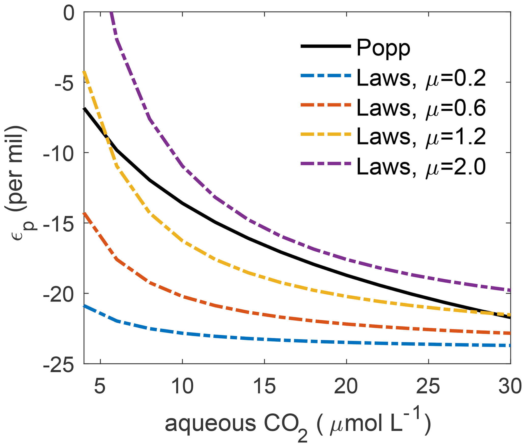
Figure 1The per mil biological fractionation factor ϵp against aqueous CO2 concentration. The solid line illustrates , in which the biological fractionation during phytoplankton growth is only a function of CO2(aq). The dashed–dotted lines show , which depends on , the ratio of phytoplankton growth rate to CO2(aq), for μ=0.2 (blue), 0.6 (red), 1.2 (yellow) and 2.0 (purple) d−1.
2.3 Model setup and experimental design
2.3.1 Setup
We conduct ocean-only simulations using the MPIOM-1.6.3p1 (Jungclaus et al., 2013; Notz et al., 2013; Mauritsen et al., 2019) with HAMOCC6. MPIOM is a free-surface ocean general circulation model. It uses a curvilinear grid with the grid poles located over Greenland and Antarctica. We use a low-resolution configuration with a nominal horizontal resolution of 1.5∘. This configuration has a minimum grid spacing of 15 km around Greenland and a maximum grid spacing of 185 km in the tropical Pacific. There are 40 unevenly spaced vertical levels. The layer thickness increases from 10 m in the upper ocean to 600 m in the deep ocean. The upper 100 m of the water column is represented by nine levels. The time step is 1 h. In this setup, we additionally include the oceanic uptake and transport of CFC-12. CFC-12 is chemically inert and can therefore be treated as a conservative and passive tracer participating in all hydrodynamical processes within the ocean identical to e.g. salinity. The implementation of the air–sea gas exchange of CFC-12 follows the OMIP protocol (Orr et al., 2017).
2.3.2 Experimental design
For the pre-industrial spin-up simulations we cyclically apply the 1905–1929 sea-surface boundary conditions from ERA20C (Poli et al., 2016, covering 1901–2010). The atmospheric CO2 mixing ratio is set to 280 ppmv. A spin-up run is first conducted without 13C tracers until the long-term averaged global net air–sea CO2 flux is smaller than 0.05 Pg C yr−1 (adequate to the C4MIP criterion for steady-state conditions of <0.1 Pg C yr−1; Jones et al., 2016). This model state is the starting point for the two spin-up runs including 13C tracers, PI_Popp and PI_Laws, which are based on the biological fractionation parameterisation (Eq. 10) and (Eq. 12), respectively.
The 13C tracers are initialised as follows. The mean δ13C of the marine organic matter is about −20 ‰ (Degens et al., 1968). Therefore, we set the initial concentrations of 13C in the bulk phytoplankton, cyanobacteria, zooplankton, dissolved organic carbon, particulate organic carbon in the water column and particulate organic carbon in the sediment to 0.98 (according to Eq. 1) of their 12C counterparts. The initial 13CDIC in the water column is calculated using the relation between δ13CDIC and PO4 (Lynch-Stieglitz et al., 1995),
and Eq. (1). Here PO4 and DIC are from the quasi-equilibrium state of the spin-up run without 13C tracers. The initial concentrations of 13C in the water column and in the sediment and the initial concentration of 13CDIC in pore water are set identical to their 12C counterparts.
The pre-industrial stable carbon isotope ratio δ13CO2 of atmospheric CO2 is fixed at −6.5 ‰. The inputs of dissolved organic 13C (DO13C) and 13CO are uniformly added at the ocean surface. The input rate of DO13C is calculated as the product of the input rate of DOC and the sea-surface ratio; the input rate of 13CO is the product of the input rate of CO and the sea-surface ratio. This approach to determine 13C input rates results in a small drift in the water-column 13C inventory, but it only has minor impact on the simulation results (see Appendix A).
PI_Popp and PI_Laws are spun up for 2500 simulation years. Equilibrium states are reached with 98 % of the ocean volume having a δ13CDIC drift of less than 0.001 ‰ yr−1 (employing the same criteria as for 14C in OMIP protocol, Orr et al., 2017). An equilibrium of the sediment is, however, not achieved for either 13C or other biogeochemical tracers.
In the transient simulations for the historical period 1850–2010, Hist_Popp and Hist_Laws, we prescribe increasing atmospheric CO2 mixing ratios (Meinshausen et al., 2017) due to anthropogenic activities and decreasing atmospheric δ13CO2 following OMIP and C4MIP protocols (Jones et al., 2016) (Fig. 2a). For the period 1850–1900, when forcing data are absent, we continue applying the 1905–1929 ERA20C cyclic forcing. From 1901 to 2010, we use the transient ERA20C forcing. The evolution of the atmospheric CFC-12 concentration (Fig. 2b) follows Bullister (2017). Because the atmospheric CFC-12 is slightly higher in the Northern Hemisphere, we prescribe a linear transition between 10∘ S and 10∘ N. Input rates of DO13C, DOC, 13CO, CO and SiO4 are kept constant and are the same as those of pre-industrial simulations.
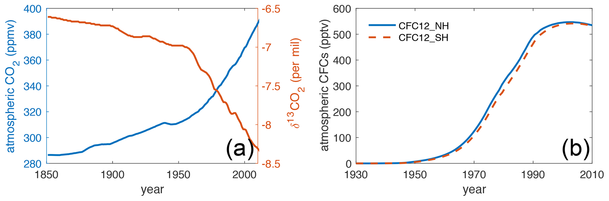
Figure 2(a) The evolution of atmospheric CO2 (blue, Meinshausen et al., 2017) and δ13CO2 (red, Jones et al., 2016) during 1850–2010. (b) The evolution of atmospheric CFC-12 concentrations (Bullister, 2017). The solid blue line indicates the Northern Hemisphere, and the dashed red line indicates Southern Hemisphere.
Our model generally simulates the physical and biogeochemical state for the present-day ocean well. The detailed model–observation comparisons for the ocean physical variables (e.g. seawater temperature and salinity, Atlantic Meridional Overturning Circulation stream function, CFC-12) and for the ocean biogeochemical tracers (e.g. primary production, nutrients, DIC) are summarised in Appendix Sects. B and C.
In this section, we compare simulated 13C between the two simulations Hist_Popp and Hist_Laws and evaluate the two experiments by comparison to observed δ13CPOC and δ13CDIC. The observations used here are the surface δ13CPOC measurements assembled by Goericke and Fry (1994) and the observed δ13CDIC, for both the surface and the interior ocean, compiled by Schmittner et al. (2013). For the model–observation comparison, we first grid the observed δ13CPOC and δ13CDIC horizontally onto a 1 × 1∘ grid and vertically (only for δ13CDIC) onto the 40 depth layers of the model. Multiple data points in the same grid cell in the same month and year are averaged. Then we bilinearly interpolate the simulated monthly-mean δ13CPOC and δ13CDIC over a 1 × 1∘ grid. To quantitatively compare the performance between Hist_Popp and Hist_Laws and to other 13C models, we calculate the spatial correlation coefficient r and the normalised root mean squared error (NRMSE, normalised by the standard deviation that is calculated using all the available measurements of δ13CPOC or δ13CDIC during the observational periods) between model results and observation.
A global ocean climatology of pre-industrial δ13CDIC has recently been derived by first estimating the oceanic 13C Suess effect (Eide et al., 2017a) and then removing it from the observed δ13CDIC (Eide et al., 2017b). This pre-industrial δ13CDIC estimate has been used to evaluate model performance (Tjiputra et al., 2020). We do not include a δ13CDIC evaluation for the pre-industrial ocean because the historical simulations in this study facilitate the direct comparison to observations in the late 20th century, which is different from Tjiputra et al. (2020), who only include pre-industrial simulations with 13C tracers. Moreover, as has already been discussed by Eide et al. (2017a) and is discussed in Sect. 5 of this study, the 13C Suess effect is possibly underestimated by the Eide et al. (2017a) approach. This suggests Eide et al. (2017b) likely overestimate the pre-industrial δ13CDIC.
3.1 Isotopic signature of particular organic carbon in the surface ocean
For comparison between Hist_Popp and Hist_Laws, the climatological mean state of δ13CPOC is derived by averaging over 1960-1991, the period when most δ13CPOC measurements were collected. In Hist_Popp, the climatological annual-mean surface δ13CPOC has a global mean value of −22.5 ‰, and it shows a distinct horizontal pattern (Fig. 3a). Less negative values up to −19.3 ‰ are found in the subtropical regions, where alkalinity is typically high and CO2(aq) is consequently low. This low CO2(aq) results in a smaller isotope fractionation during carbon fixation by phytoplankton (Eq. 10, Fig. 1) with a biological fractionation factor ‰ (Fig. 3c). Poleward of the subtropical regions, δ13CPOC gradually decreases. The reason for this is twofold. First, ϵp decreases from −13 ‰ to about −20 ‰ following the increase in CO2(aq). Second, the thermal effect of equilibrium fractionation causes about 3 ‰ more fractionation in the polar regions than in the tropical and subtropical regions (according to Eqs. 7 and 9). The lowest δ13CPOC of about −30 ‰ occurs close to Antarctica where highest surface DIC concentrations are typically found because of the upwelling of deep waters and the reduced air–sea gas exchange by ice cover (Takahashi et al., 2014). The annual range of δ13CPOC (Fig. 3e), i.e. the difference between the minimum and the maximum of its climatological monthly-mean annual cycle, is low (<0.5 ‰) in the subtropical regions, and it increases polewards up to ∼9 ‰ in the Southern Ocean, mirroring meridional changes in the annual range of CO2(aq).
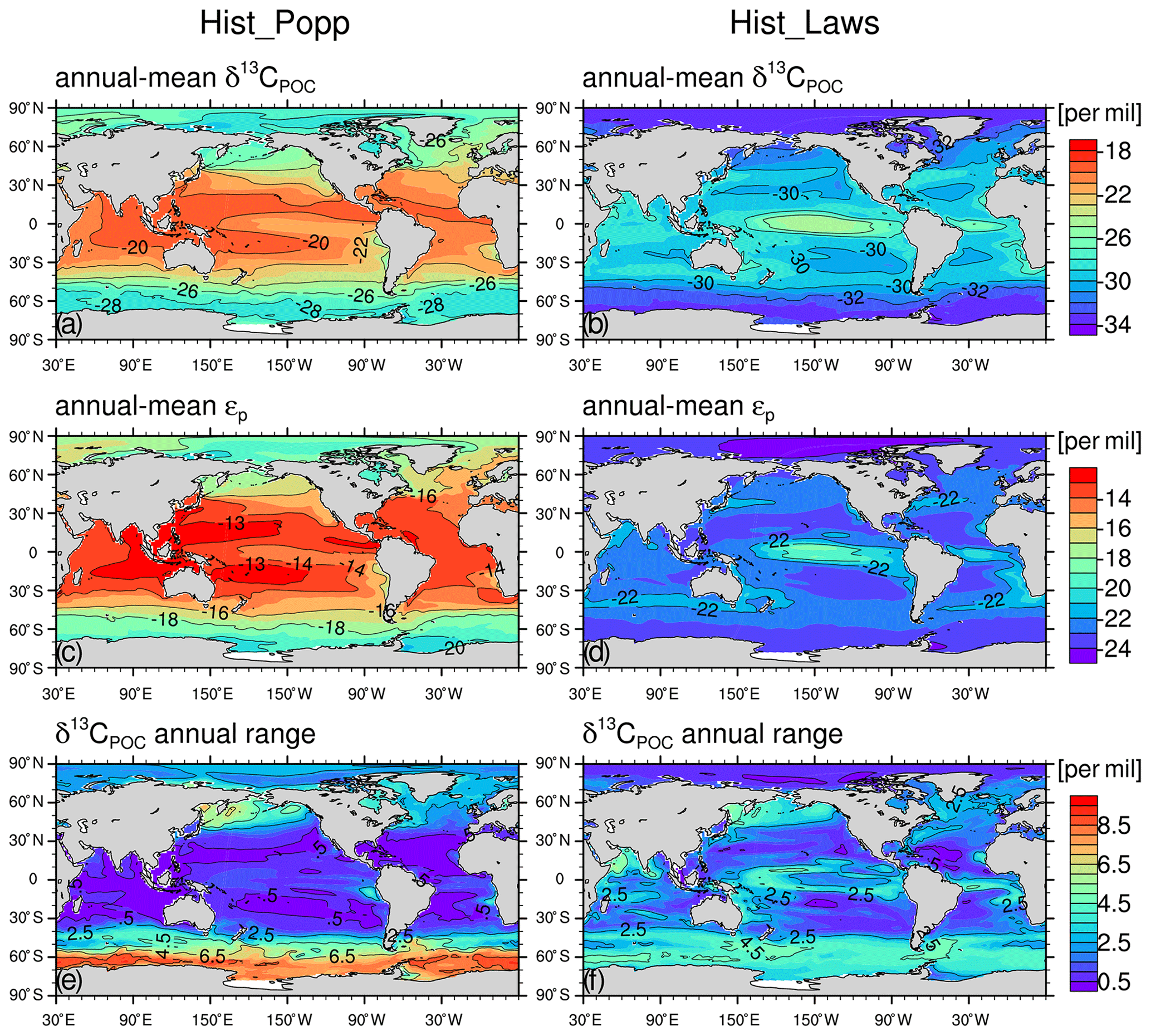
Figure 3The climatological (1960–1991) annual-mean surface values for Hist_Popp (a, c, e) and Hist_Laws (b, d, f) for δ13CPOC (a, b), ϵp (c, d), and for the annual range of δ13CPOC (e, f). All values are given in per mil (‰).
Compared to Hist_Popp, Hist_Laws shows lower annual-mean surface δ13CPOC (Fig. 3b), with a global-mean value of −29.9 ‰ due to more negative ϵp (Fig. 3d). This is because (Fig. 1) is always more negative than when the simulated mean growth rates (Fig. C1a and b) are lower than 1 d−1. As increases with growth rate (Eq. 12), we find less negative δ13CPOC (up to −24.1 ‰) in the central tropical Pacific, where highest growth rates are simulated (Fig. C1a and b). The lowest δ13CPOC of −33 ‰ occurs in the Arctic Ocean and around Antarctica due to the combination of low growth rate, high CO2(aq) and low seawater temperature. The meridional range of the annual-mean δ13CPOC in Hist_Laws (∼9 ‰) is smaller than that of Hist_Popp (∼11 ‰) because for low growth rates is generally less sensitive to CO2(aq) changes compared to (Fig. 1). This also results in a smaller annual range of δ13CPOC in high latitudes (Fig. 3f) than Hist_Popp (Fig. 3e). In the low and mid-latitudes, Hist_Laws shows larger annual range of δ13CPOC because in these regions CO2(aq) concentrations are relatively stable but growth rates shows noticeable seasonal variability.
Hist_Popp captures major features of the observed δ13CPOC (Fig. 4a, c and e). The meridional gradient, with less negative values in the low latitudes and minimal values around 60∘ S, is well reproduced. In contrast, Hist_Laws shows generally lower δ13CPOC than the observations (a global mean bias of −8 ‰) and a smaller δ13CPOC difference between low and high latitudes (Fig. 4b, d and f). This is also seen in a recent study by Dentith et al. (2020), who tested and with the FAst Met Office/UK Universities Simulator (FAMOUS). The underestimation in the global mean and in the meridional gradient of δ13CPOC in Hist_Laws suggests that the parameters of the linear fit in Eq. (12) (slope and intercept) would need to be increased to gain a better performance. Around 60∘ S of the Atlantic Ocean (Fig. 4b), Hist_Laws simulates a smaller range of δ13CPOC than the observations. This is also a result of the small δ13CPOC annual range produced by (Fig. 3f). Between 40∘ S and 40∘ N in the Atlantic Ocean, Hist_Laws simulates δ13CPOC peaks in the region of high growth rates south of the Equator, whereas the observed high δ13CPOC values are located between the Equator and 20∘ N.
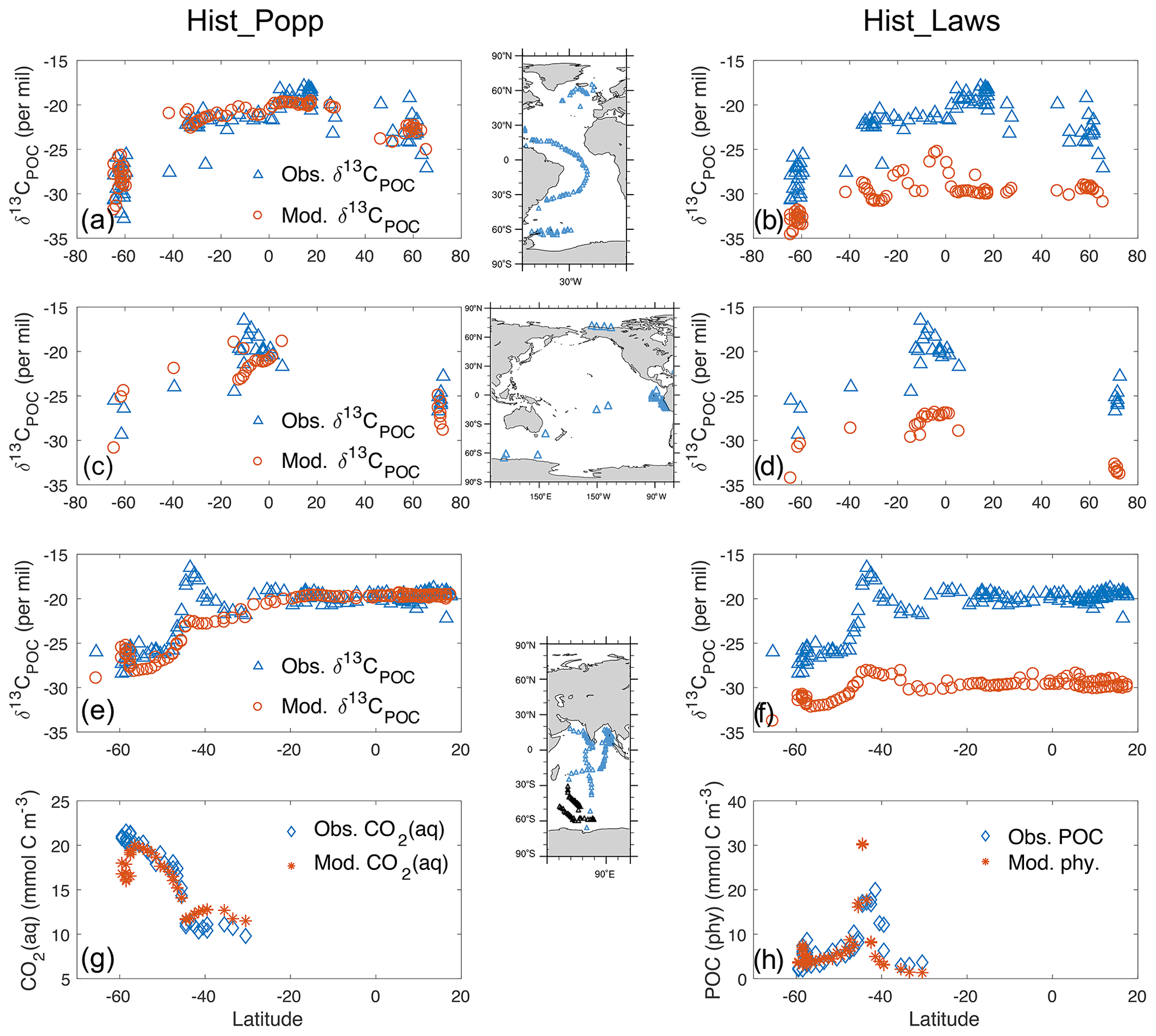
Figure 4Comparison of surface δ13CPOC (‰) observations (blue triangle) from Goericke and Fry (1994) to model data (red circle) in Hist_Popp (a, c, e) and Hist_Laws (b, d, f) for the Atlantic, Pacific and Indian Ocean, respectively. Inserted maps show cruise tracks of the measuring campaigns. (g) Comparison of simulated CO2(aq) (red star) to observations (blue diamond) in the South Indian Ocean (Francois et al., 1993; measurement locations indicated by black triangles in the inset map for the Indian Ocean). Panel (h) is as panel (g) but for particulate organic matter, represented by total POC in Francois et al. (1993) and by phytoplankton biomass in the model. The measurement precision is ±0.17 ‰ for δ13CPOC and 2 % for CO2(aq) and particulate organic matter, according to Francois et al. (1993).
In the Indian Ocean around 45∘ S, Hist_Popp does not capture the prominent δ13CPOC peak in the field data (Fig. 4e), despite the fact that the simulated CO2(aq), the controlling factor in the parameterisation (Eq. 10), well reproduces the meridional variation of the contemporaneous CO2(aq) measurements (Fig. 4g). Although the empirical correlation between ϵp and CO2(aq), such as Eq. (10), holds true to the first order over large areas of the global ocean, other factors, such as growth rate, affect the local variability in ϵp (Popp et al., 1998; Hansman and Sessions, 2016; Tuerena et al., 2019). Hist_Laws captures the δ13CPOC peak around 45∘ S in the observations (Fig. 4f), owing to the dependency of on phytoplankton growth rate and to the model successfully reproducing the high productivity in this region (illustrated by phytoplankton biomass, Fig. 4h). This is in alignment with the field study by Francois et al. (1993) and the model study by Hofmann et al. (2000), who ascribed this observed δ13CPOC peak to a local high phytoplankton production during the measurement period.
Overall, Hist_Popp (r=0.84 and NRMSE=0.57) better reproduces the observed δ13CPOC than Hist_Laws (r=0.71, NRMSE=2.5). Here a higher NRMSE indicates the model captures a smaller fraction of the variation in observations. The performance of Hist_Popp regarding δ13CPOC compares well to that of the FAMOUS model (Dentith et al., 2020; comparing their Fig. 8 and Fig. 4 in this study) and the University of Victoria (UVic) Earth System Model of intermediate complexity (with r=0.74 and NRMSE=0.92; Schmittner et al., 2013). Note that Schmittner et al. (2013) compared climatological annual-mean model output to the δ13CPOC measurements from Goericke and Fry (1994), whereas our study uses model results of the corresponding month and year of the measurements. This difference leads to a better comparison of Hist_Popp to the observed δ13CPOC in high latitudes, particularly in the South Atlantic Ocean around 60∘ S, and therefore it is one reason for the slight better performance of Hist_Popp compared to Schmittner et al. (2013), aside from the underlying differences between the two models.
Hist_Popp also well reproduces the temporal changes of the biological fractionation factor ϵp when compared to the observation-based estimates of Young et al. (2013). In Hist_Popp, the change rate of ϵp has a global-mean value of −0.026 ‰ yr−1 for the period 1960–2009 (Fig. C7a), similar to an estimate of −0.022 ‰ yr−1 in Young et al. (2013). Modest ϵp changes are found in eastern tropical Pacific and south of 60∘ S, in good agreement with Young et al. (2013). Hist_Laws, on the other hand, shows a very small global-mean ϵp change rate of −0.005 ‰ yr−1 (Fig. C7b) as is less sensitive to the increase in CO2(aq) than .
3.2 Isotopic signature of dissolved inorganic carbon δ13CDIC
3.2.1 Comparison between Hist_Popp and Hist_Laws and to observations
Figures 5a–b and 6a–f compare the climatological annual mean of δ13CDIC (averaged over 1990–2005, when most δ13CDIC measurements were collected) between Hist_Popp and Hist_Laws. The two simulations exhibit very similar δ13CDIC patterns for both the surface and interior ocean. The surface seawater DIC is enriched in 13C due to the preferential uptake of the light isotope 12C by phytoplankton during primary production. As particulate organic matter sinks and is remineralised at depth, the negative δ13CPOC signal is released. Consequently, in both Hist_Popp and Hist_Laws, δ13CDIC at the surface is generally higher than in the ocean interior. At the surface of the equatorial central Pacific, the eastern boundary upwelling systems and the Southern Ocean south of 60∘ S, lower δ13CDIC (<1.6 ‰) is seen due to the upward transport of the 13C-depleted water (Fig. 5a and b). In the interior ocean, we find higher δ13CDIC (>1 ‰) in well-ventilated water masses, in particular the North Atlantic Deep Water (NADW) (Fig. 6a and d). The lowest δ13CDIC values ‰) occur at depth in tropical and subtropical regions (Fig. 6a–f), where a large amount of organic matter is remineralised.
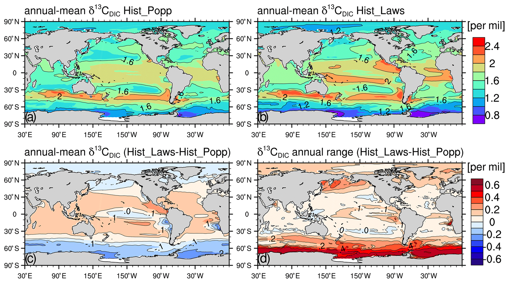
Figure 5Climatological (averaged over 1990–2005) annual-mean surface δ13CDIC for Hist_Popp (a) and Hist_Laws (b), respectively. Panels (c) and (d) show the difference in the climatological annual-mean δ13CDIC between Hist_Laws and Hist_Popp, and the difference in the climatological annual range of δ13CDIC between the two simulations, respectively.
The global-mean surface δ13CDIC of the two experiments only differs marginally (1.64 ‰ for Hist_Popp and 1.7 ‰ for Hist_Laws), which is expected as they are run using the same prescribed atmospheric δ13CO2 (Schmittner et al., 2013). Given very similar mean surface DI13C, the larger vertical DI13C gradients in Hist_Laws, established by more negative δ13CPOC (Fig. 3a and b), yield lower DI13C concentration at depth. This adjustment of DI13C content in the ocean interior takes place during the pre-industrial spin-up phase of the simulations via air–sea 13CO2 exchange (Appendix A). At the end of the 2500-year spin-up, the water-column DI13C inventory in PI_Laws is 1.1×10¹² kmol lower than PI_Popp, yielding a global mean δ13CDIC difference of 0.25 ‰ (Fig. 6g–i). Such interior-ocean δ13CDIC difference caused by using different parameterisation for biological fractionation is also seen in Jahn et al. (2015) and Dentith et al. (2020). The seasonal upward transport of the lower deep-ocean δ13CDIC in Hist_Laws leads to lower annual-mean surface δ13CDIC and larger δ13CDIC annual range in regions of upwelling (Fig. 5c and d).

Figure 6Zonal-mean δ13CDIC of the Atlantic Ocean (a, d, g), the Pacific Ocean (b, e, h) and the Indian Ocean (c, f, i) for Hist_Popp (a–c), Hist_Laws (d–f) and for the difference between Hist_Laws and Hist_Popp (g–i).
When compared to the observed δ13CDIC, Hist_Popp (r=0.81, NRMSE=0.7) has a slightly better performance than Hist_Laws (r=0.80, NRMSE=1.1). Hist_Laws generally shows vertical gradients of δ13CDIC that are too strong and therefore δ13CDIC values that are too low in the ocean interior, as is seen in the depth profiles of horizontally averaged δ13CDIC (Fig. 7). This points to too strong a preference for the isotopically light carbon simulated by as is already discussed in Sect. 3.1. Given the slightly better performance of Hist_Popp than Hist_Laws regarding δ13CDIC, we focus in the following on the comparison between Hist_Popp and observed δ13CDIC.
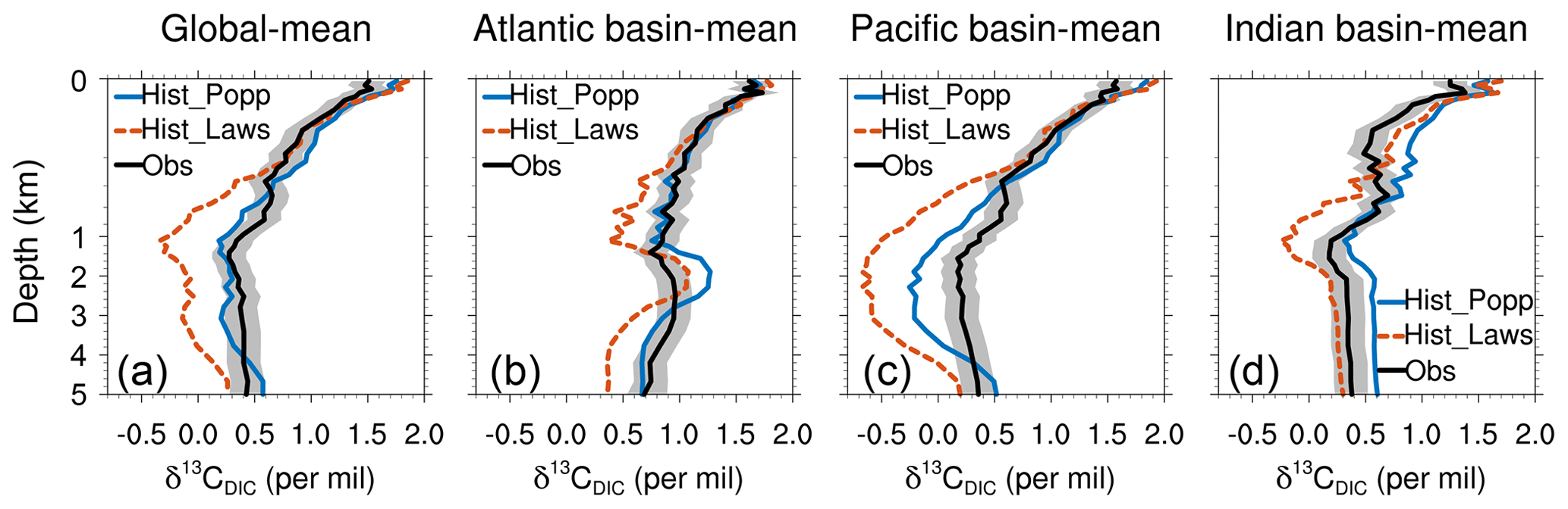
Figure 7Depth profiles of horizontally averaged δ13CDIC of Hist_Popp (solid blue line), Hist_Laws (dashed red line) and the observational data from Schmittner et al. (2013) (solid black line) for the global ocean (a), the Atlantic Ocean (b), the Pacific Ocean (c) and for the Indian Ocean (d). The grey shading indicates observation uncertainty of ±0.15 ‰, which relates to the estimated accuracy due to unresolved intercalibration issues between laboratories (0.1 ‰–0.2 ‰; Schmittner et al., 2013).
3.2.2 Source of surface δ13CDIC biases in Hist_Popp
Figure 8 contains model–observation comparison for the surface δ13CDIC. Overall, the magnitude and spatial distribution of the observed δ13CDIC is well-captured by Hist_Popp. In the surface ocean, the mean δ13CDIC is slightly overestimated by Hist_Popp (1.7 ‰ compared to 1.5 ‰ in observation). Positive biases are widely seen in the Indian and Pacific Ocean, and the negative biases are mostly found in the Atlantic Ocean (Fig. 8c). To better understand the source of differences between model and observations, we follow the method of Broecker and Maier-Reimer (1992) to decompose δ13CDIC into a biological component δ13C and a residual component δ13C, driven by air–sea exchange and ocean circulation:
Here the subscript M.O. refers to mean ocean values, Δphoto is the carbon isotope fractionation during marine photosynthesis and RC:P is the C:P ratio of marine organic matter. We use ‰ (Eide et al., 2017b) and (Takahashi et al., 1985) for both model and observational data. In reality Δphoto shows spatial variability due to the variations of CO2(aq) (Fig. 3c) and temperature (Eq. 7) at the sea surface. However, using a constant Δphoto only has limited quantitative impact on the model–observation comparison of the two components. To calculate δ13C from observations, we employ δ13C ‰, mmol m−3 (Eide et al., 2017b) and PO4 from the World Ocean Atlas (WOA13; Garcia et al., 2013a). Considering the strong seasonality in PO4 in the surface ocean, we select the phosphate concentration from the climatological monthly WOA data (available only for the upper 500 m of the water column) and the climatological monthly-mean model data for the same month as the δ13CDIC observations. The observed mean ocean phosphate concentration PO mmol m−3 is obtained by first merging the time mean of the PO4 monthly WOA data in the upper 500 m and the PO4 annual-mean WOA data below 500 m and then mapping the combined data to the vertical grid of our model. For simulated δ13C, the model data of δ13C ‰, mmol m−3, mmol m−3 and PO4 are used. The model–observation δ13C difference is calculated by subtracting the model–observation δ13C difference from the model–observation δ13CDIC difference.
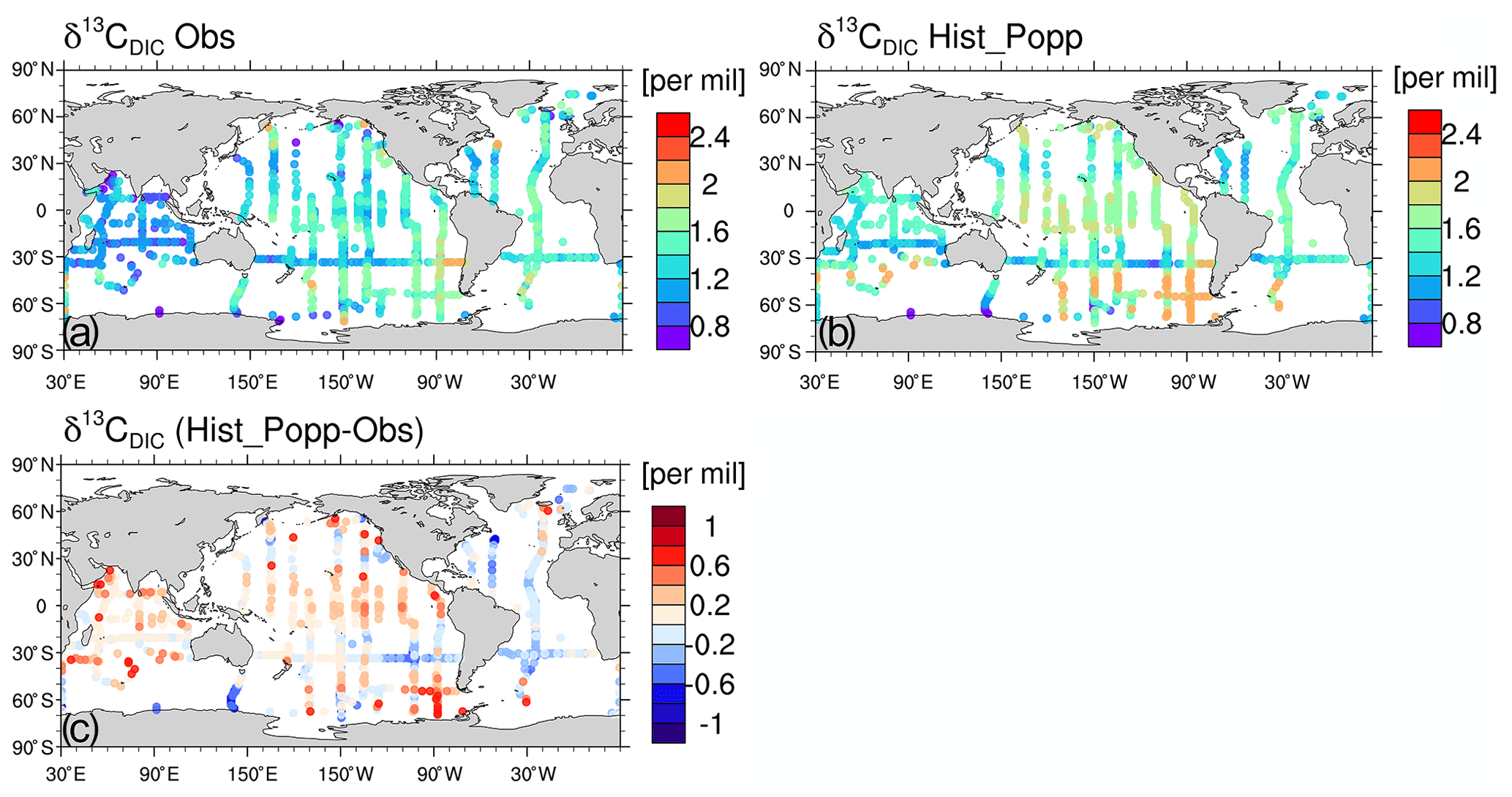
Figure 8Observed surface δ13CDIC (Schmittner et al., 2013) (a) and simulated δ13CDIC in Hist_Popp sampled at the location, month and year of the observation (b). (c) The difference in δ13CDIC between Hist_Popp and observations.
The model captures the major features of the observed δ13C at the surface; that is, higher values are seen in the subtropical regions and lower values in the high latitudes (Fig. C8a and b). Nevertheless, noticeable quantitative differences exist (Fig. 9a), which resemble the distribution of ) bias (Fig. 9b). Between 30∘ N and 30∘ S in the surface ocean, we find a mean negative bias of about −0.1 ‰. This is caused by the underestimation of primary production in the subtropical gyres (due to the underestimation of phytoplankton growth rates; see Appendix C1) and the consequently reduced enrichment of 13C in surface DIC. A strong positive δ13C bias of 0.6 ‰ to 1 ‰ is seen in the North Pacific, where in the model iron is not a limiting nutrient (Fig. C3), in contrast to observations (Moore et al., 2013). In the equatorial central Pacific, a weak positive δ13C bias <0.2 ‰ is caused by a primary production that is too high. Specifically, the simulated phytoplankton growth rates in this region compare well to observations, whereas the simulated phytoplankton biomass is too high (Appendix C1). The latter is mainly induced by an upwelling that is too strong. The observed mean upward vertical velocity at 0, 140∘ W and 60 m depth during May 1990–June 1991 is m s−1 (Weisberg and Qiao, 2000), whereas the model simulates m s−1 for the same location and period.

Figure 9Model–observation difference in the biological component δ13C (a), (b), and the residual component δ13C (c) at the ocean surface. (d) The net air–sea CO2 flux (positive into the air, averaged over 1990–2005) difference between the model data and observation-based data product from Landschützer et al. (2015).
In the Southern Ocean, a strong positive δ13C bias of 0.6 to 1 ‰ (Fig. 9a) results from a primary production that is too high under surface iron concentrations that are too high (0.2–0.4 nmol L−1 compared to generally <0.25 nmol L−1 from data of the GEOTRACES programme (http://www.geotraces.org, last access: 15 April 2021, not shown). Primary production is limited by iron only south of 50∘ S in the model compared to south of 40∘ S from observation (Moore et al., 2013). One cause for the high surface iron concentration is that in HAMOCC6 organic matter is remineralised at depths that are too shallow. This can been seen from the positive apparent oxygen utilisation (AOU) biases above 500 m south of 45∘ S (Fig. 10j–l).
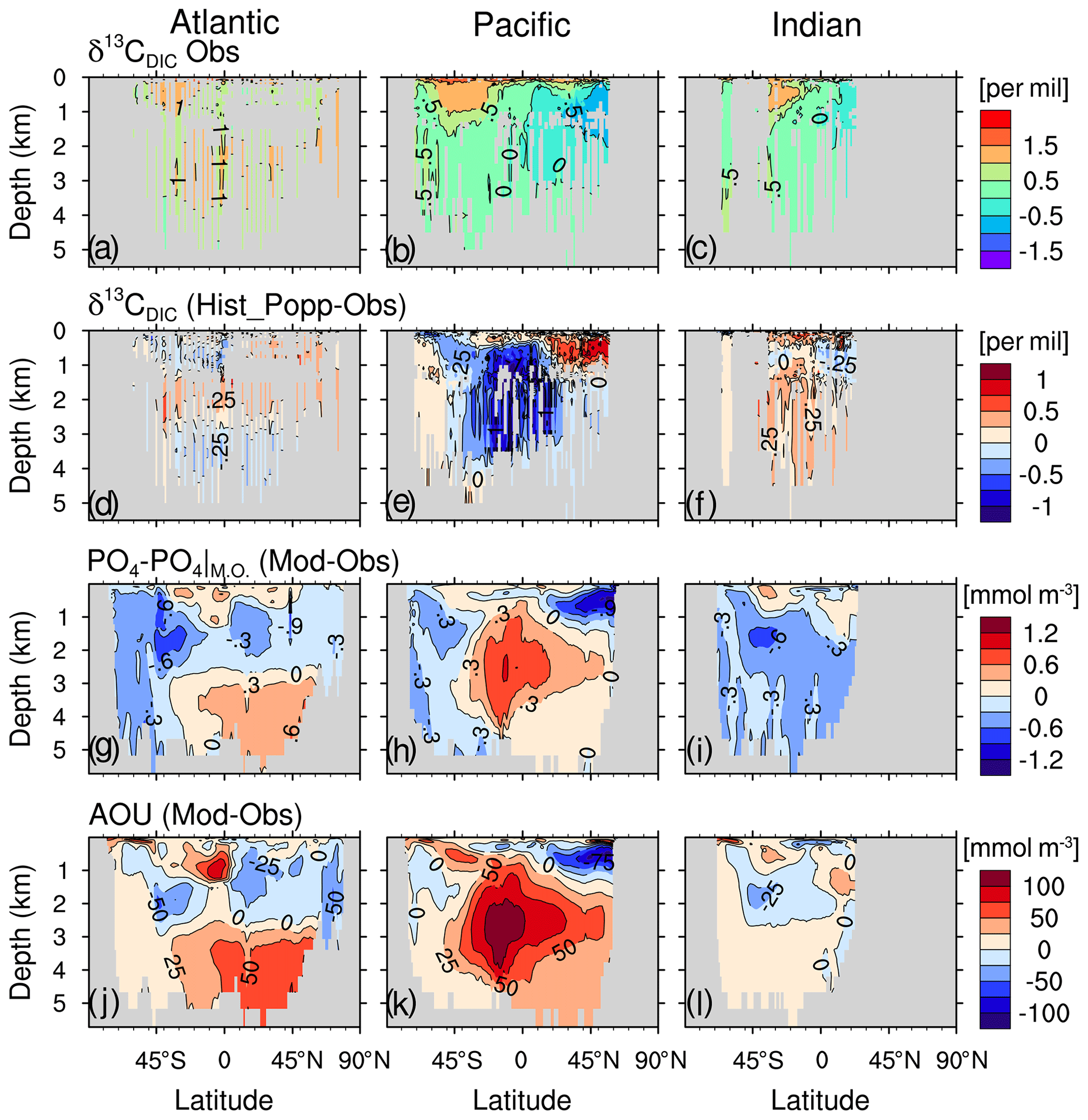
Figure 10Zonal-mean distribution in the Atlantic Ocean (left column), the Pacific Ocean (middle column) and the Indian Ocean (right column) for the δ13CDIC observations from Schmittner et al. (2013) (a–c), for the difference between Hist_Popp (sampled at the same location, year and month of the observations) and δ13CDIC measurement (d–f), for the difference between model and WOA data (WOA13; Garcia et al., 2013a) (g–i), and for the apparent oxygen utilisation (AOU) difference between model and WOA data (WOA13; Garcia et al., 2013b) (j–l). Here the climatological annual mean values of PO4 and AOU are used for both model and WOA data because seasonal variation is negligible in the interior ocean and WOA only provides monthly data above 500 m.
Another reason for the high surface iron concentration in the Southern Ocean is that MPIOM simulates an upwelling that is too strong. In particular, below 1000 m, the simulated upward velocity shows noticeably larger magnitude m s−1, Fig. B4) than that of a dynamically consistent and data-constrained ocean state estimate (see Fig. 1 in Liang et al., 2017). The upwelling that is too strong in the model is consistent with the volume transport that is too large across the Drake Passage of 192 Sv compared to 134–173 Sv from observations (Nowlin Jr. and Klinck, 1986; Cunningham et al., 2003; Meredith et al., 2011; Donohue et al., 2016). Our model also features larger downward velocities than the estimate from Liang et al. (2017), which correspond to mixed layer depths that are too deep in the Southern Ocean (up to 3000 m, Fig. B5) than observations (<700 m; de Boyer Montégut et al., 2004; Holte et al., 2017).
We find strong δ13C negative biases of −0.5 ‰ to −1 ‰ (Fig. 9c) in the North Pacific and the Southern Ocean, which partially compensate for the positive biases of δ13C (Fig. 9a) in these regions. One major cause for the negative δ13C bias in these two regions is our model overestimating the uptake of anthropogenic carbon, as is illustrated by the net air–sea CO2 difference between the model and the observation (Fig. 9d). Consequently, the decreased atmospheric ratio over the industrial period further lowers δ13CDIC in the two ocean regions in the model. In the Southern Ocean, the upward transport of 13C-depleted water is too large, which also contributes to a negative δ13C bias.
3.2.3 Source of δ13CDIC biases in the interior ocean of Hist_Popp
Figure 10 contains the model–observation comparison for zonal-mean δ13CDIC in the Atlantic, Pacific and Indian Ocean. In the interior ocean, δ13CDIC is controlled by remineralisation of 13C-depleted organic matter and by ocean circulation (Broecker and Peng, 1993; Lynch-Stieglitz et al., 1995; Schmittner et al., 2013). Low δ13CDIC is often found in waters of high nutrient concentration and vice versa. Thus, we find positive (negative) δ13CDIC biases coincide with negative (positive) phosphate biases (Fig. 10d–i). In the Atlantic Ocean between 1000 and 3000 m, the North Pacific above 1500 m and the Indian Ocean below 1000 m, positive δ13CDIC biases and negative phosphate biases are mainly caused by a remineralisation that is too low, as is shown by the negative AOU biases (Fig. 10j–l).
North of 30∘ S in the Atlantic Ocean, the negative δ13CDIC biases below 3000 m, together with the positive δ13CDIC biases between 1000 and 3000 m, suggest δ13CDIC vertical gradients that are too strong in the model (Fig. 10d). This results from a lower boundary of the NADW cell that is too shallow, constantly located above 2800 m (Fig. B3), compared to an estimated NADW lower boundary of about 4300 m deep at 26∘ N (Msadek et al., 2013; Smeed et al., 2017). A possible reason for the shallow NADW in the model is that the Lower North Atlantic Deep Water (LNADW), forming from the Denmark Strait Overflow Water and the Iceland–Scotland Overflow Water, is not dense enough to flow further southward. This can be seen from the CFC-12 distribution along the zonal Sect. A5 at 24∘ N (Fig. B7). The observed deeper CFC-12 maximum (3000–4500 m west of 60∘ W) indicates the presence of LNADW (Dutay et al., 2002), which is not represented in our model.
We find the strongest negative δ13CDIC bias in the deep eastern equatorial Pacific (Fig. 10e). The cause is the “nutrient trapping” problem in the model, characterised by nutrient concentrations that are too high in the deep eastern equatorial Pacific (Fig. 10h), which is a persistent problem in many ESMs (Aumont et al., 1999; Dietze and Loeptien, 2013). Based on sensitivity experiments with the Geophysical Fluid Dynamics Laboratory model and the UVic model, Dietze and Loeptien (2013) concluded the primary cause of the nutrient trapping problem is likely model biases in physical ocean state – in particular, the poor representation of the Equatorial Intermediate Current system and equatorial deep jets. The latter two current systems are indeed poorly represented in our model as well. Specifically, the zonal current at 1000 m depth (typical depth for the Equatorial Intermediate Current system) shows too little spatial variability and too low speeds of ∼0.2 cm s−1 (Fig. B6), compared to the observed alternating jets with a meridional scale of 1.5∘ and speeds of ∼5 cm s−1 (see Fig. 2 from Cravatte et al., 2012).
The performances of both Hist_Popp and Hist_Laws regarding δ13CDIC are comparable with the Norwegian Earth System Model version 2 (NorESM2, Tjiputra et al., 2020; comparing their Fig. 21), the Commonwealth Scientific and Industrial Research Organisation Mark 3L climate system model with the Carbon of the Ocean, Atmosphere and Land (CSIRO Mk3L-COAL), Pelagic Interactions Scheme for Carbon and Ecosystem Studies (PISCES) and LOch-Vecode-Ecbilt-CLio-agIsm Model (LOVECLIM) (see Table 2 and Figs. 3, S2 and S3 of Buchanan et al., 2019, and references therein), the Community Earth System Model (CESM, Jahn et al., 2015; comparing their Figs. 5 and 6 to our Figs. 7 and 6, respectively), and the UVic Earth System Model (Schmittner et al., 2013). The latter two studies used the same δ13CDIC data set for model evaluation. Schmittner et al. (2013) reported a better performance (r=0.88 and NRMSE=0.5) than ours (r=0.81 and NRMSE=0.7 in Hist_Popp). One main reason is that the nutrient trapping problem in HAMOCC6 does not occur in the simulations of Schmittner et al. (2013).
The oceanic δ13C measurements taken during the late 20th century already include a signal that originates from burning of isotopically light fossil fuel over the industrial period. The associated decrease in atmospheric δ13C (Fig. 2) affects oceanic δ13C via air–sea gas exchange, leading to a general decrease in δ13CDIC. The distribution of this δ13CDIC change, i.e. the oceanic 13C Suess effect, could serve as benchmark for ocean models to evaluate the uptake and re-distribution of the anthropogenic CO2 emissions in the ocean.
The model is able to reproduce the size of the global oceanic anthropogenic CO2 sink, though some local biases in the net air–sea CO2 flux exist (Fig. 9d). The simulated sink by year 1994 is 99 Pg C, which compares well to the observation-based estimate of 118±19 Pg C from Sabine et al. (2004) and to other model estimates (e.g. 94 Pg C in Tagliabue and Bopp, 2008). For a direct comparison to published studies, we calculate the oceanic δ13C Suess effect, δ13CSE, as the difference between the 1990s-averaged δ13CDIC from Hist_Popp and the pre-industrial climatological (50-year mean) δ13CDIC from PI_Popp. δ13CSE calculated using the results of Hist_Laws and PI_Laws only shows a marginal difference (global mean <0.04 ‰) and is therefore not presented.
The surface mean δ13CSE in this study is −0.66 ‰, similar to the model study of Schmittner et al. (2013) (−0.67 ‰) and to the estimate by Sonnerup et al. (2007) ‰), who used an observation-based approach. The strongest oceanic 13C Suess effect is found in the subtropical gyres in the model (Fig. 11a), where water masses have long residence times at the ocean surface and therefore receive a strong anthropogenic imprint (Quay et al., 2003). In the subtropical gyres, the simulated surface δ13CSE generally varies between −0.8 ‰ and −1.1 ‰, which compares well to the surface ocean δ13C decrease of ‰ recorded by coral and sclerosponges (Wörheide, 1998; Böhm et al., 1996, 2000; Swart et al., 2002, 2010) and to the estimates of ‰ extracted from GLODAPv2 (Olsen et al., 2016; Eide et al., 2017a).

Figure 11The simulated oceanic Suess effect δ13CSE from the pre-industrial period to the 1990s at sea surface (a) and at 200 m (b).
Along the vertical sections A16, P19 and I8S9N, δ13CSE is mainly confined to the upper 1000 m depth in the subtropical gyres of the South Atlantic, the Pacific Ocean and the Indian Ocean (Fig. 12a–c). In the North Atlantic, δ13CSE penetrates deeper than the other ocean regions, due to the intensive ventilation related to the formation of NADW. The simulated δ13CSE distributions show similar features to those of CFC-12 (Fig. B8). This is because both the decrease in δ13CDIC and increase in CFC-12 in the ocean are predominantly caused by the uptake of atmospheric anthropogenic signals and the subsequent transport by ocean circulation. Since changes in δ13CDIC are also induced by changes in marine biological activity, we separate δ13CDIC into a component depicting changes due to the transport of the surface 13C signal, i.e. the “preformed” δ13CDIC, and to a regenerated component δ13Creg, following Sonnerup et al. (1999):
The ratio is 122:172 in HAMOCC6, and we use the simulated δ13CPOC for δ13Corg. Clearly, the change in the preformed component dominates δ13CSE (comparing Fig. 12a–c to Fig. 12d–f). A major difference between δ13C and δ13CSE is that positive δ13C is widely seen below 1000 m, particularly in the Pacific Ocean (Fig. 12e). These positive δ13C values relate to changes in the regenerated component δ13Creg (see Appendix D).
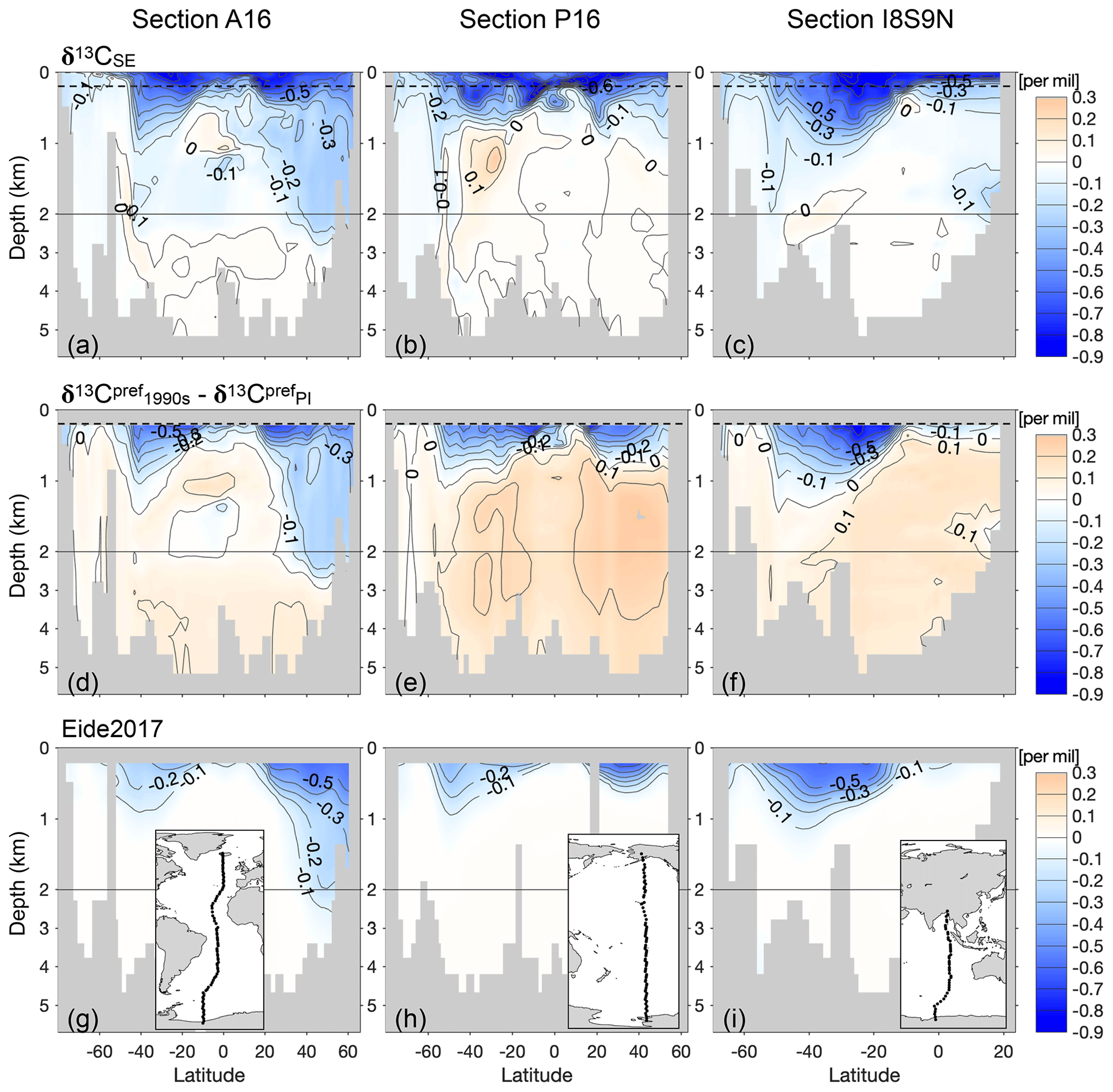
Figure 12The simulated oceanic Suess effect δ13CSE since pre-industrial times for vertical sections A16 in the Atlantic Ocean (a), P16 in the Pacific Ocean (b) and I8S9N in the Indian Ocean (c). Panels (d)–(f) and (g)–(i) are as panels (a)–(c) but for the change in the preformed component and for the observation-based estimate of the oceanic Suess effect from Eide et al. (2017a), respectively. Inserted maps show the location of the vertical sections. The horizontal dashed black lines in panels (a)–(f) indicate 200 m depth, below which the Eide et al. (2017a) estimate is available. Note the bathymetry is different between the model and Eide et al. (2017a).
Eide et al. (2017a) (hereafter E17) derived the first observation-based estimate of the global ocean 13C Suess effect since pre-industrial times. E17's approach uses the concept of the similarity between the oceanic uptake of the anthropogenically produced CFC-12 and isotopically light CO2 (see details in Appendix E1). Due to method- and data-specific limitations E17 stated that they potentially underestimate the oceanic 13C Suess effect. However, based on observations alone it is not possible to gain insight into the spatial distribution of this uncertainty or into its origin.
Our model simulations, particularly PI_Popp and Hist_Popp, provide an opportunity to learn more about the source of this uncertainty because the oceanic δ13C in the late 20th century (Sect. 3), the oceanic anthropogenic CO2 sink (Sect. 4) and the invasion of CFC-12 into the ocean (Fig. B8) are well represented. Moreover, our simulated δ13CSE qualitatively resembles the oceanic 13C Suess effect estimate of E17 (see comparison between Fig. 11b and E17's Fig. 7, as well as comparison between Fig. 12a–c and g–i).
Based on the similarity between the oceanic uptake of the atmospheric CFC-12 and δ13CO2 signal, E17 link the 13C Suess effect since 1940 (when CFC-12 becomes detectable in the ocean) to CFC-12 partial pressure (pCFC-12) with a proportionality factor. Under the assumption of a temporally constant regenerated fraction δ13Creg, this proportionality factor is considered equivalent to the slope of a linear regression relationship between the preformed component δ13Cpref and pCFC-12 at any time after 1940. Thus, this slope a can be obtained by performing linear regression for field measurements of δ13Cpref and pCFC-12. Multiplying a and pCFC-12 data yields the 13C Suess effect since 1940, which is then scaled to the full industrial period by a constant factor fatm (Eq. E7) related to changes in the atmospheric δ13C signature:
Here a is the regression slope for the linear relationship between δ13C and pCFC-12t (Eq. E5). The value of a is determined for each ventilation region defined in E17 (i.e. the Indian Ocean, North Pacific, South Pacific, North Atlantic and South Atlantic). Details of the E17 approach are given in Appendix E1.
By applying E17's approach to our model data that are sampled at the same geographical locations as observations used in E17, we obtain the regression slopes, hereafter referred to as apref, for each ventilation region. Taking year t=1994 we obtain the estimated oceanic 13C Suess effect, SEpref, for the period from the pre-industrial to 1994 following Eq. (16). The detailed calculation of SEpref is given in Appendix E2.
To quantify if SEpref under- or overestimates the oceanic 13C Suess effect, we compare SEpref to the simulated oceanic 13C Suess effect . Figure 13a presents (SEpref−SEMod) for 200 m depth. Positive values of(SEpref−SEMod) indicate underestimation of the oceanic 13C Suess effect.

Figure 13Distribution at 200 m depth for SEpref−SEMod (a), SEpref−SEtotal (b) and SEtotal−SEMod (c). The isoline increment is 0.2 ‰. In panels (b) and (c), the South Pacific Ocean is not presented because the relationship between the total oceanic 13C Suess effect δ13CSE(1994–1940) and pCFC-121994 is too weak (r2=0.07), and therefore SEtotal can not be estimated (see Appendix E4).
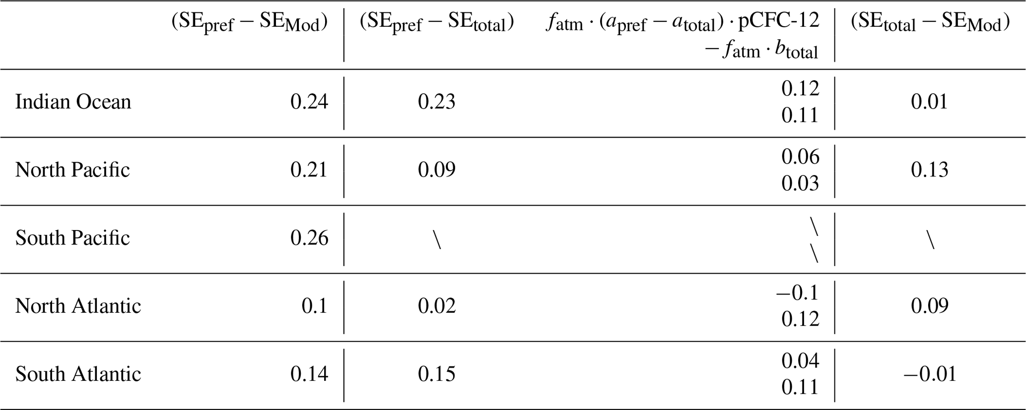
At 200 m SEpref mostly underestimates SEMod (Fig. 13a). The region-mean underestimation is 0.24 ‰ for the Indian Ocean, 0.21 ‰ for the North Pacific, 0.26 ‰ for the South Pacific, 0.1 ‰ for the North Atlantic and 0.14 ‰ for the South Atlantic (Table 1). Our model findings are very similar to the underestimation range discussed by E17. They determined an uncertainty range of 0.15 ‰ to 0.24 ‰ by comparing their global-mean estimate (−0.4 ‰ at 200 m depth) to an estimate (−0.55 ‰ to −0.64 ‰ at 200 m) which they deduced from previous model studies. Specifically, based on Broecker and Peng (1993) and Bacastow et al. (1996) E17 assumed an ocean-to-atmosphere ratio of the 13C Suess effect of 0.65 and the 200 m to surface ratio of the 13C Suess effect of 0.6–0.7. Multiplying the above two ratios with the atmospheric δ13CO2 decrease of −1.4 ‰ by year 1994 yields the global-mean 13C Suess effect estimate of −0.55 ‰ to −0.64 ‰ at 200 m. In our model, the global-mean surface-ocean–atmosphere ratio of the 13C Suess effect is only 0.46, significantly lower than the five-box model of Broecker and Peng (1993). The 200 m to surface ratio of the 13C Suess effect is 0.75 in our model, and it is slightly higher than that of Bacastow et al. (1996), who employed an ocean general circulation model with coarse vertical resolution (four layers for the upper 200 m).
Table 1Region-mean (SEpref−SEMod), (SEpref−SEtotal) and (SEtotal−SEMod) for five ventilation regions defined by E17, i.e. the Indian Ocean, North Pacific, South Pacific, North Atlantic and South Atlantic. The unit is per mil. (SEpref−SEtotal) is further decomposed into the two contributions and according to Eq. (20).
5.1 Source of underestimation attributed to data coverage
E17 have speculated that the major cause of the underestimation of the oceanic 13C Suess effect is that the available observations are mostly from the intermediate and deep waters. The ocean–atmosphere equilibration timescale for δ13C (10 years, Broecker and Peng, 1974) is significantly longer than that of pCFC-12 (1 month, Gammon et al., 1982). Thus, waters that have a shorter surface residence time, such as the deep waters ventilated in the South Hemisphere, would show less negative regression slope apref (for the linear relationship between δ13Cpref and pCFC-12, Eq. E5) than waters that have a longer surface residence time, e.g. subtropical gyres. In other words, apref for the subtropical gyre water should be more negative than apref for the entire corresponding ventilation region (the North Pacific, South Pacific, North Atlantic, South Atlantic or the Indian Ocean).
We test this potential explanation for the Indian Ocean and North Pacific. We are able to span regressional relationships for the subtropical gyres only because we have a larger data base. Specifically, we consider only model data at the geographical location of observations, but we use all model levels between 200 m and the pCFC-12 penetration depth (see Appendix E3). For the Indian Ocean, we combine model data from Subtropical Gyre Water (STGW) and Sub-Antarctic Mode Water (SAMW) as both water masses have a strong 13C Suess effect (Eide et al., 2017a). We find for this combined water mass (STGW) apref (, r2=0.49) is more negative than that for the whole ventilation region , Fig. E3a). So indeed, with additional observations in the subtropical gyre we would receive a stronger 13C Suess effect estimate for the Indian Ocean. However, this difference in apref only corresponds to an underestimation of about 0.12 ‰ at 200 m for the Indian subtropical region (see calculation in Appendix E3), which does not explain the total underestimation of 0.24 ‰ in the Indian Ocean (Table 1). In the North Pacific apref for the Subtropical Gyre Water , r2=0.26) is even less negative than that for the whole ventilation region in the model, which is in contrast to the conjecture of E17.
5.2 Source of underestimation attributed to assumptions of E17's approach
A potential under-representation of data from subtropical gyres does not fully explain the underestimation of the 13C Suess effect found in our model. Instead, we argue that the source of uncertainty mainly relates to different assumptions that have been made in the E17 approach. Specifically, in the expression of the preformed component δ13C (following Eq. E3),
E17 assume that the regenerated component is constant in time, i.e. . Consequently, Eq. (17) is reduced to
Furthermore, they assume that the regression slope apref for δ13C and pCFC-121994 is equivalent to the regression slope for the total 13C Suess effect δ13CSE(1994−1940) and pCFC-121994 (see Eqs. E1, E4 and E5). This implies that the preformed component δ13C of 1940 has to be spatially uniform.
However, we find a specific vertical structure in the simulated δ13C (Fig. 14a–c). Over large regions of the ocean, δ13C generally decreases with increasing depth. This vertical distribution of δ13Cpref is already present in pre-industrial times. High surface δ13CDIC caused by biological fractionation is transported into the ocean interior. Therefore, the preformed component generally decreases with increasing water depth. From pre-industrial times to 1940, the decrease in the atmospheric ratio is relatively small (0.4 ‰, Fig. 2a), and therefore also the impact on the oceanic δ13CDIC is small. Thus, δ13C has the similar vertical structure as that of the pre-industrial ocean.
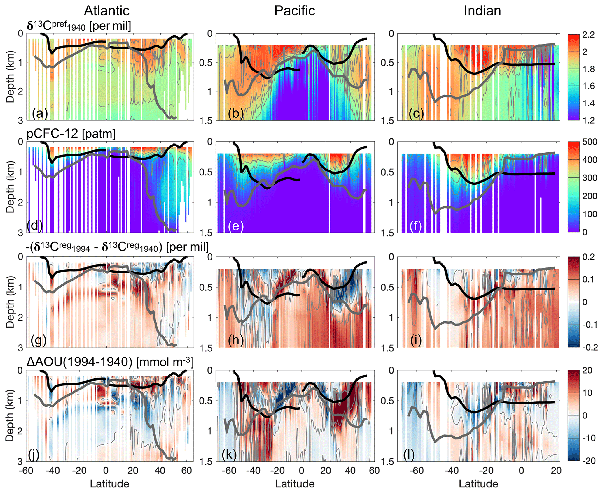
Figure 14(a–c) The zonal mean of the simulated δ13C for the locations where both observed CFC-12 and δ13CDIC are available. The thick grey line is the pCFC-121994=20 patm isoline, above which model data are used to perform linear regression. The thick black lines outline the Subtropical Gyre Water in the Atlantic and North Pacific Ocean, as well as the Subtropical Gyre Water and Sub-Antarctic Mode Water in the Indian Ocean and South Pacific Ocean (definition of water masses in Table E1). Panels (d)–(f), (g)–(i) and (j)–(l) are as panels (a)–(c) but for pCFC-121994, for and for AOU changes between year 1940 and 1994, respectively. Note that for the Atlantic Ocean the upper 3 km is shown, whereas for the Pacific and Indian Ocean the upper 1.5 km is presented.
Both the total δ13CSE(1994−1940) (mostly negative, similar to the distribution of δ13CSE(1990s−PI) in Fig. 12a–c) and pCFC-12 (Fig. B8a–c) show larger absolute values at the surface than in the interior ocean. As δ13C is more positive in the upper ocean than the deep ocean, δ13C has a smaller vertical gradient than δ13CSE(1994−1940) (see Eq. 18). Thus, a linear regression for δ13C and pCFC-12 results in a less negative slope than a slope obtained with a spatially uniform δ13C, which implicates a contribution to an underestimation of the oceanic 13C Suess effect.
We also find that is non-zero, and it shows considerable spatial variability (Fig. 14g–i). Most prominently, in the North Atlantic is mostly negative above 500 m, and it is mostly positive below 500 m. This vertical structure of in the North Atlantic leads to stronger vertical gradient in δ13C and therefore a more negative regression slope than that obtained with . This implies the overestimation of the 13C Suess effect in the North Atlantic.
To evaluate the impact of assuming a spatially uniform δ13C and , we calculate an estimated 13C Suess effect from pre-industrial times to 1994, SEtotal, based on a linear regression for the simulated total oceanic 13C Suess effect δ13CSE(1994−1940) and pCFC-12:
Here atotal and btotal are regression coefficients for δ13CSE(1994−1940) and pCFC-12 (more details in Appendix E4). With Eqs. (16) and (19) we get
Comparison between the regressional slope apref (obtained for δ13C and pCFC-12) and atotal facilitates the quantification of the under- or overestimation of the 13C Suess effect linked to the above two assumptions.
In the Indian Ocean (Fig. E2a) is less negative than (Fig. E3a). This results in an underestimation of 0.12 ‰ according to Eq. (20). Similarly, for the North Pacific (Fig. E2b) is less negative than (Fig. E3b), which leads to an underestimation of 0.06 ‰. For the South Atlantic (Fig. E2e) and (Fig. E3e), which yields an underestimation of 0.04 ‰. Such underestimation is mainly due to the decreasing δ13C with increasing depth in these regions.
Different from these three ventilation regions, in the North Atlantic (Fig. E2d) is more negative than (Fig. E3d). This is due to the specific vertical structure of as previously discussed.
Another major difference between SEpref and SEtotal is the non-negligible negative intercept btotal (Eq. 20). This reveals the underestimation of SEpref related to E17's assumption that the 13C Suess effect is directly proportional to pCFC-12. The intercept btotal emerges possibly due to the different atmospheric time history of the 13C Suess effect compared to CFC-12, as is discussed by E17 for the deep ocean with very low or zero CFC-12. The decreasing of δ13CPOC under increasing surface CO2(aq) (Appendix D) also contributes to an non-negligible btotal as lower δ13CPOC leads to lower δ13CDIC in the ocean interior. In the South Atlantic and Indian Ocean, ‰ corresponds to an underestimation of 0.12 and 0.11 ‰ (Table 1), respectively.
Table 1 summaries of the contributions from (SEpref−SEtotal) for different ventilation regions. The comparison to the total underestimation given by (SEpref−SEMod) shows that this underestimation, which is attributed to the assumption of E17's approach, is the largest contributor for the Indian Ocean and the South Atlantic.
The residual under-/overestimation of SEpref given by shows how well a method based on linear regression relationships between δ13CSE and pCFC-121994 can estimate the global ocean Suess effect. (SEtotal−SEMod) at 200 m generally show positive values, i.e. underestimation, in low latitudes (between 40∘ S and 40∘ N), and it is rather negative poleward of 40∘ (Fig. 13c). This pattern results from pooling data from different water masses to generate one regression relationship for a large ventilation region. The waters ventilated in lower latitudes typically have a stronger 13C Suess effect than those ventilated in high latitudes. This is clearly reflected in the linear regression relationships between δ13CSE(1994–1940) and pCFC-121994 for the North Atlantic (Fig. E3d), which shows that the regression slope atotal for the Subtropical Gyre Water is noticeably steeper than that of the deep waters. Accordingly in the interior ocean, the water masses ventilated in the low latitudes generally show an underestimation of the 13C Suess effect (positive values of SEtotal−SEMod), and the water masses ventilated in the high latitudes show an overestimation (Fig. E1g–i). In the North Atlantic Ocean, the region-mean underestimation ‰ is predominantly contributed by ‰. In the North Pacific Ocean ‰ accounts for more than half of the total underestimation 0.21 ‰. In the Indian and South Atlantic Ocean, however, (SEtotal−SEMod) has hardly any influence to the region-mean underestimation.
In summary, our analysis points out two major causes for the underestimation of 13C in E17's approach. The first is the assumption of a spatially uniform preformed δ13C component in 1940. The second cause is the neglect of processes not directly linked to the oceanic uptake and transport of CFC-12, e.g. the uptake of anthropogenically light CO2 in the times prior to the emission of CFC-12 and the decrease in δ13CDIC due to the decrease in δ13CPOC over the industrial period.
We present results of the new 13C module in the ocean biogeochemical model HAMOCC6 for the historical period forced by reanalyses data (ERA20C). We test two parameterisations of different complexity for the biological fractionation factor: depends on dissolved CO2 (Popp et al., 1989); is a function of dissolved CO2 and phytoplankton growth rate (Laws et al., 1995). Furthermore, we use our consistent model framework to assess the approach by Eide et al. (2017a), which yields the first global oceanic 13C Suess effect estimate based on a correlation between preformed δ13CDIC and CFC-12 partial pressure.
The comparison between simulated and observed isotopic ratio of organic matter δ13CPOC reveals that (r=0.84 and NRMSE=0.57) has a better performance than (r=0.71 and NRMSE=2.5). Using results in noticeably lower δ13CPOC values and smaller δ13CPOC gradients between low and high latitudes compared to observations. The parameterisation of Laws et al. (1995), obtained based on cultures of marine diatom Phaeodactylum tricornutum, results in too strong a preference of isotopically light carbon in our global ocean biogeochemical model.
Regarding δ13CDIC, also yields slightly better agreement with observations than (r=0.81 and NRMSE=0.7 versus r=0.80 and NRMSE=1.1), because produces lower δ13CPOC and therefore lower interior-ocean δ13CDIC than those found in observations. performs well considering the uncertainties in observed δ13CDIC (0.1 ‰–0.2 ‰; Schmittner et al., 2013). Our model slightly overestimates surface δ13CDIC. By decomposing δ13CDIC into a biological component and a residual component, we find the overestimation in the high-latitude ocean is dominated by biases in the biological component caused by e.g. surface iron concentration that is too high. In the interior-ocean δ13CDIC biases are mainly due to biases in the physical state (for instance, a boundary that is too shallow between the NADW cell and the Antarctic Bottom Water cell in MPIOM).
Our model represents well the temporal evolution of the oceanic δ13CDIC since pre-industrial times, i.e. the oceanic 13C Suess effect due to the intrusion of isotopically light carbon into the ocean. With the complete information on the spatial and temporal 13C evolution in the ocean, together with the simulated evolution of CFC-12, we identify the sources for the potential uncertainties in the framework of Eide et al. (2017a) for deriving an observation-based oceanic 13C Suess effect. Based on our model, we find underestimations of the 13C Suess effect at 200 m by 0.24 ‰ in the Indian Ocean, 0.21 ‰ in the North Pacific Ocean, 0.26 ‰ in the South Pacific Ocean, 0.1 ‰ in the North Atlantic Ocean and 0.14 ‰ in the South Atlantic Ocean. These numbers are in line with the underestimation range 0.15 ‰ to 0.24 ‰ conjectured by Eide et al. (2017a). They speculated this underestimation is due to the under-representation of the water masses with a stronger 13C Suess effect, such as the Subtropical Gyre Water and Sub-Antarctic Mode Water, in the observational data. Our analysis shows that their hypothesis only explain half of the underestimation in the Indian Ocean. For the North Atlantic Ocean this hypothesis is not supported by the model data . We identify two major causes for the underestimation of the 13C Suess effect by the applied method. The first relates to the assumption of a spatially uniform preformed component of δ13CDIC in year 1940. In our model this preformed component is generally more positive in the upper ocean than in the interior ocean, which contributes to the underestimation of the δ13C Suess effect. The second cause relates to the neglect of processes that are not directly linked to the oceanic uptake and transport of CFC-12 – for instance, the 13C Suess effect prior to the emission of CFC-12 and the decrease in δ13CPOC over the industrial period.
We conclude that the new 13C module with biological fractionation factor from Popp et al. (1989) has a satisfactory performance. We are aware that the parameterisation omits any potential changes, e.g. in ecosystem structure, which might have occurred in the paleo-ocean. Our new 13C module will serve as a useful tool to evaluate the performance of MPI-ESM in paleoclimate and to investigate the past changes in the ocean, for instance within the ongoing research project PalMod (Latif et al., 2016).
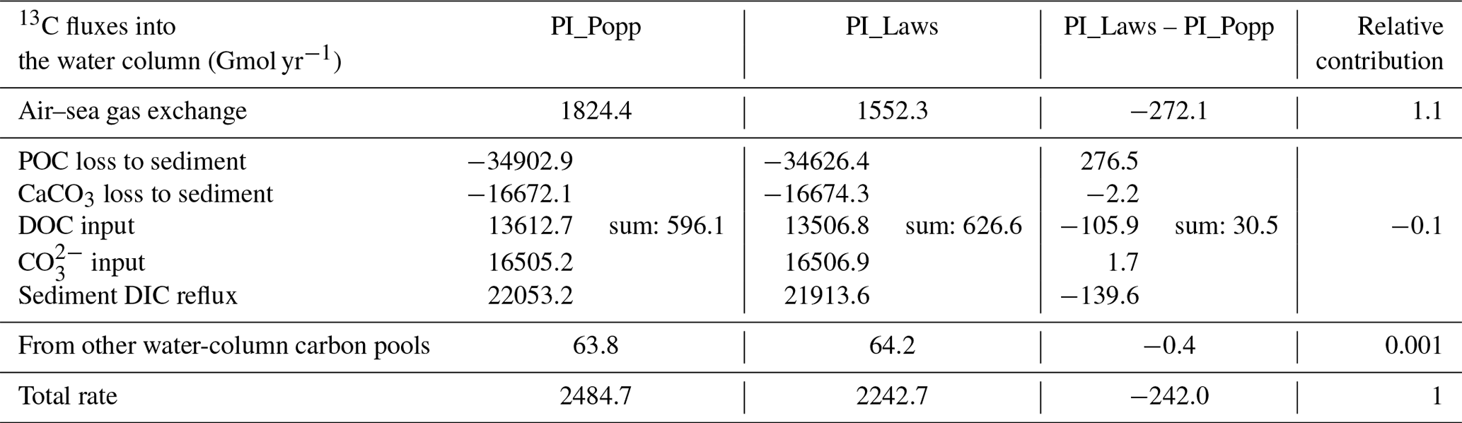
The water-column DI13C inventory difference is primarily a result of the difference in the net air–sea 13CO2 flux between PI_Popp and PI_Laws. This is demonstrated by the comparison of the contributions of the governing factors for the water-column DI13C inventory changes (Table A1), including air–sea gas exchange, loss of POC and CaCO3 to marine sediment, diffusion of the remineralised DIC from sediment into the water column, input of DOC and CO, and the exchange with other marine carbon pools (phytoplankton, CaCO3, etc.). Table A1 also reveals that the current method to determine the 13C input (see Sect. 2.3.2) only has a small contribution to the change in the water-column DI13C inventory.
Table A1Contributions to the rate of the water-column DI13C inventory change (in Gmol yr−1), averaged in the last 50 years in the corresponding pre-industrial spin-up simulations. Positive values denote contributions to the increase in the water-column DI13C inventory. The last column gives the relative contribution to the total rate difference with relative contribution = (PI_Laws-PI_Popp) / total rate difference.
Sea surface temperature (SST) and salinity (SSS) generally show good performance (Fig. B1 and Table B1). The most striking bias is seen for SSS (2–3 psu) in the Arctic Ocean. In the ocean interior, the performance of temperature and salinity is similar to other ocean general circulation models, e.g. Tjiputra et al. (2020) (comparing our Table B1 to their Fig. 2). The model biases shown here (for instance, the surface layers are too cold, whereas the water between 500 and 2500 m is too warm and saline; see Fig. B2) are typically seen in MPIOM; see Jungclaus et al. (2013) for a detailed discussion.

Figure B1Biases in sea surface temperature (SST, panel a) and salinity (SSS, panel b). Both model and observational data (EN4 version 4.2.0; Good et al., 2013) are averaged for 1960–1999.
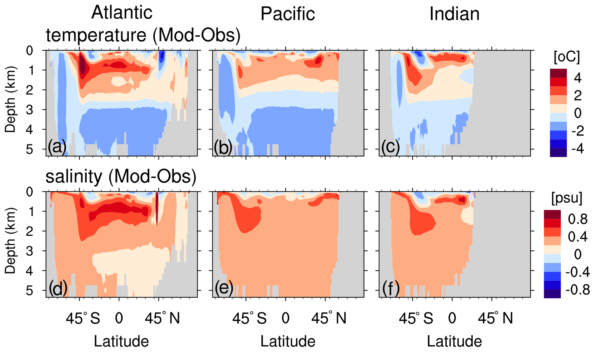
Figure B2Zonal-mean biases of seawater temperature (a–c) and salinity (d–f) with respect to observations (EN4 version 4.2.0; Good et al., 2013) for the Atlantic Ocean (a, d), Pacific Ocean (b, e) and Indian Ocean (c, f).
Table B1Summary of the spatial correlation coefficient r and normalised root mean square error (NRMSE) between model data and observations from EN4 (version 4.2.0; Good et al., 2013).
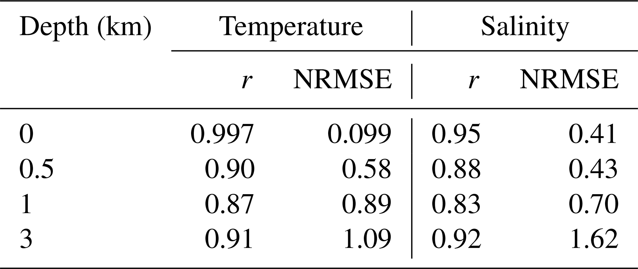
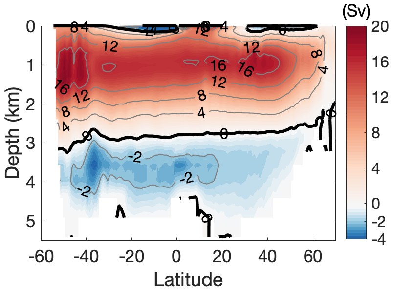
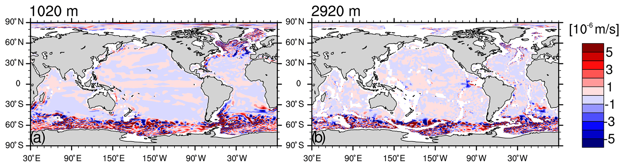
Figure B41990–2009 mean vertical velocity (m s−1) in the model at 1020 m depth (a) and 2920 m depth (b).
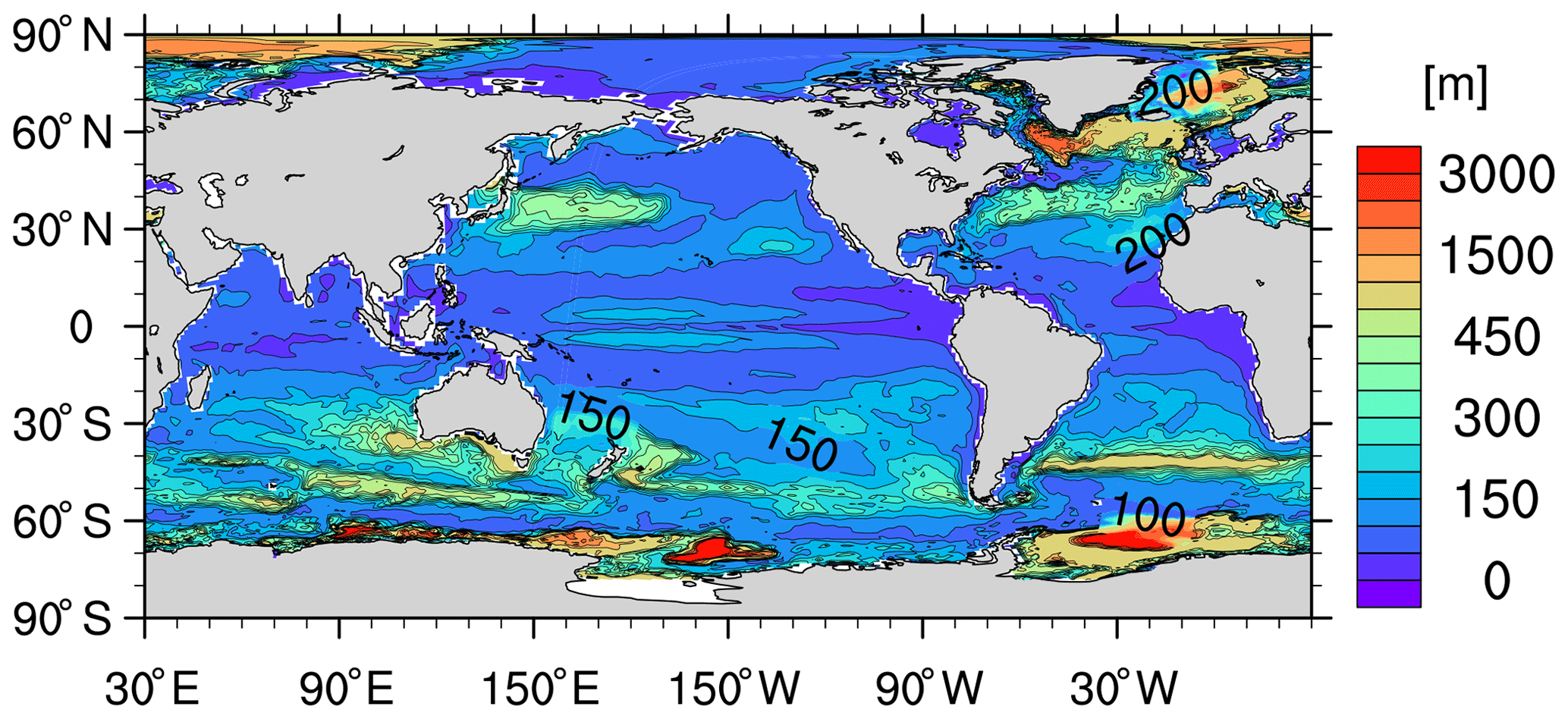
Figure B5The mean of the annual maximum of the monthly mixed layer depth (m) for the period 1970–1999 in the model. The mixed layer depth is defined as the depth at which a 0.03 kg m−3 change in potential density with respect to the surface has occurred. Contour intervals are 50 for 0–500 and 500 for 500–3000.
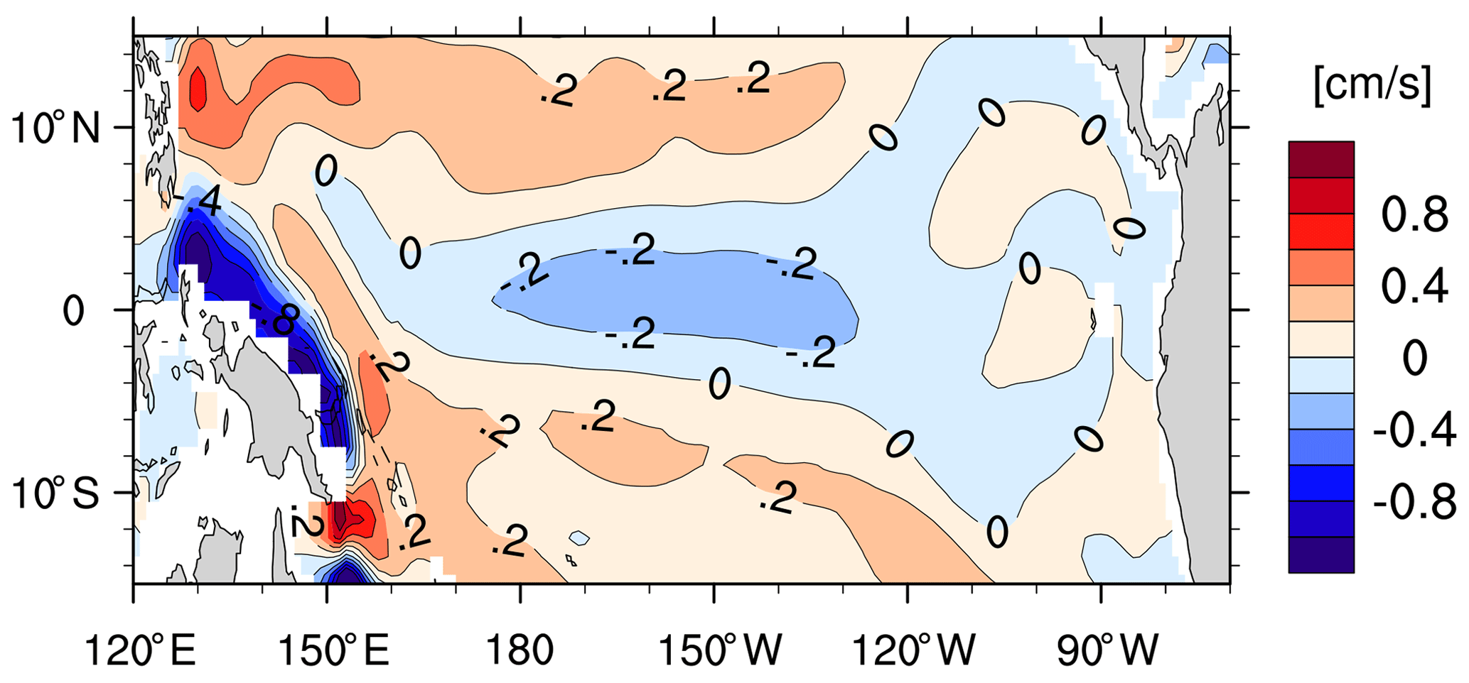
Figure B6The simulated zonal current (cm s−1) at 960 m depth in the equatorial Pacific (averaged over January 2003–August 2009). Positive values indicate eastward flow.
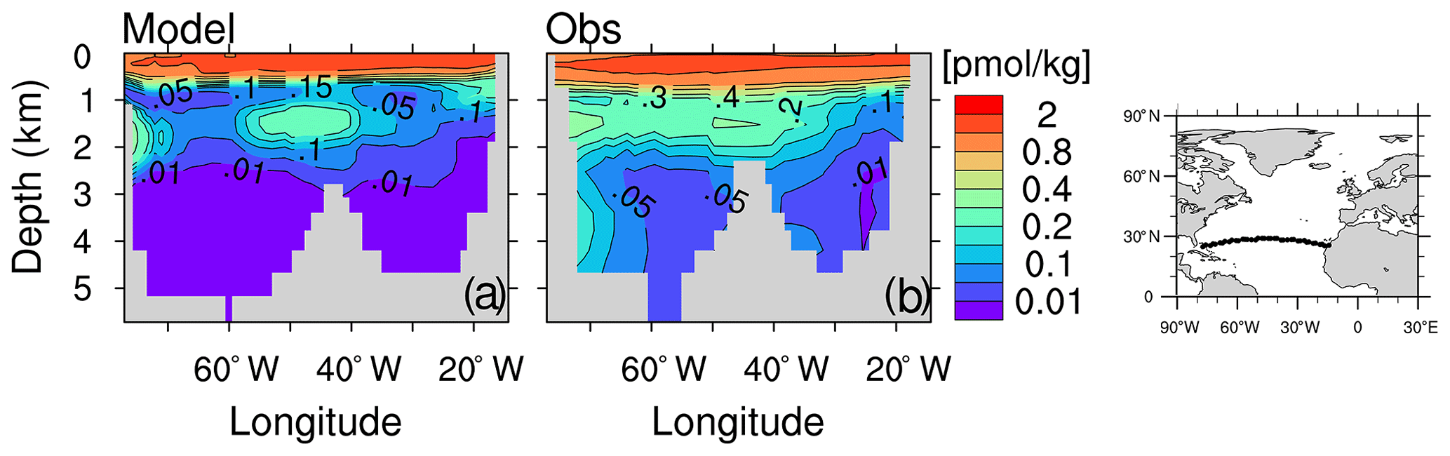
Figure B7CFC-12 concentration (pmol kg −1) in February 1998 along the A5 section in the Atlantic Ocean (see right panel) of the model (a) and of observations from GLODAPv1 database (panel b; Key et al., 2004). Contour intervals are 0.01, 0.05, 0.1, 0.15, 0.2, 0.3, 0.4, 0.6, 0.8, 1.2 and 2 pmol kg −1.
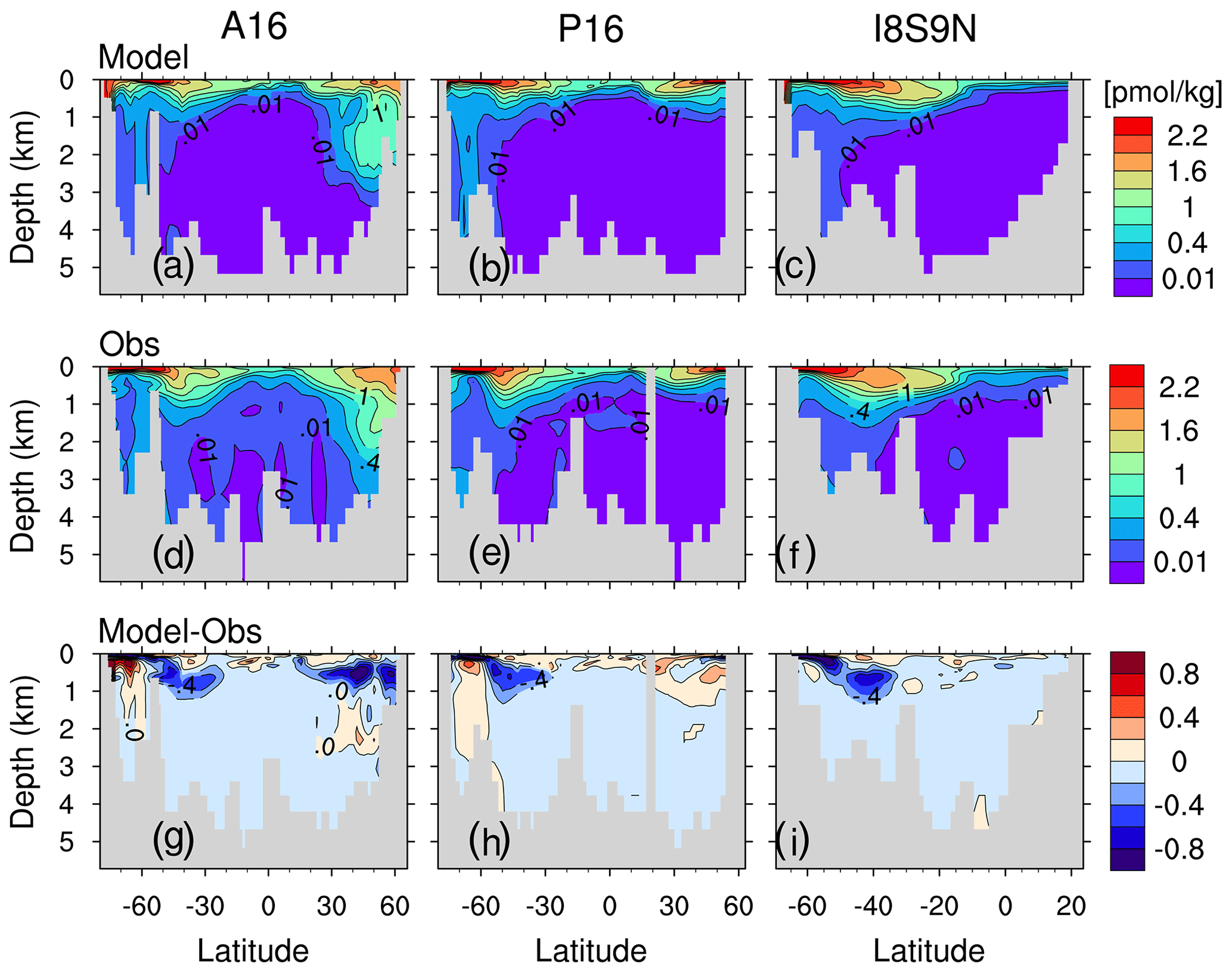
Figure B8(a–c) CFC-12 concentration (pmol kg −1) for the section A16 (a), P16 (b) and I8S9N (c). Panels (d)–(f) and (g)–(i) are as panels (a)–(c) but for the observed CFC-12 (GLODAPv1; Key et al., 2004) and for the difference between model and observation, respectively. The isolines in panels (a)–(f) are 0.01, 0.1, 0.4, 0.7, 1.0, 1.3, 1.6, 1.9 and 2.2 pmol kg−1. The isoline increment in panels (g)–(i) is 0.2 pmol kg−1.
C1 Net primary production, growth rate, biomass and limiting nutrients
The simulated net primary production, 48.7 Gt yr−1 for bulk phytoplankton and 3 Gt yr−1 for cyanobacteria, compares well with the satellite-based estimate of ∼52 Gt yr−1 (Westberry et al., 2008; Silsbe et al., 2016).
The simulated growth rate μ (Fig. C1a and b, only shown for bulk phytoplankton because cyanobacteria has a much lower primary production) is broadly consistent with the large-scale patterns of the satellite-based μ estimates from Westberry et al. (2008) (Figs. C1c and C1d) and with field observations. In the central equatorial Pacific the simulated μ well reproduces the observed range (0.55–0.7 d−1, Chavez et al., 1996; note the satellite-based estimates overestimate μ due to excluding iron limitation). In the subtropical gyres, the simulated μ (annual-mean 0.1–0.25 d−1) is at the lower side of both the observations (annual mean 0.3–0.53 d−1 in the North Pacific subtropical gyre, Letelier et al., 1996; annual mean 0.13–0.62 d−1 in the North Atlantic subtropical gyre, Marañón, 2005) and the satellite-based μ estimates. In the Pacific sector of the Southern Ocean, the simulated μ (0.3–0.4 d−1) in the austral summer is higher than the observations (about 0.1–0.2 d−1; Boyd et al., 2000) and the satellite-based estimates. The simulated phytoplankton biomass is too high in the equatorial Pacific (>100 mg C m−3) and the Southern Ocean (>50 mg C m−3; Fig. C2) compared to the satellite-based estimates (<30 mg C m−3 for both regions; Westberry et al., 2008).
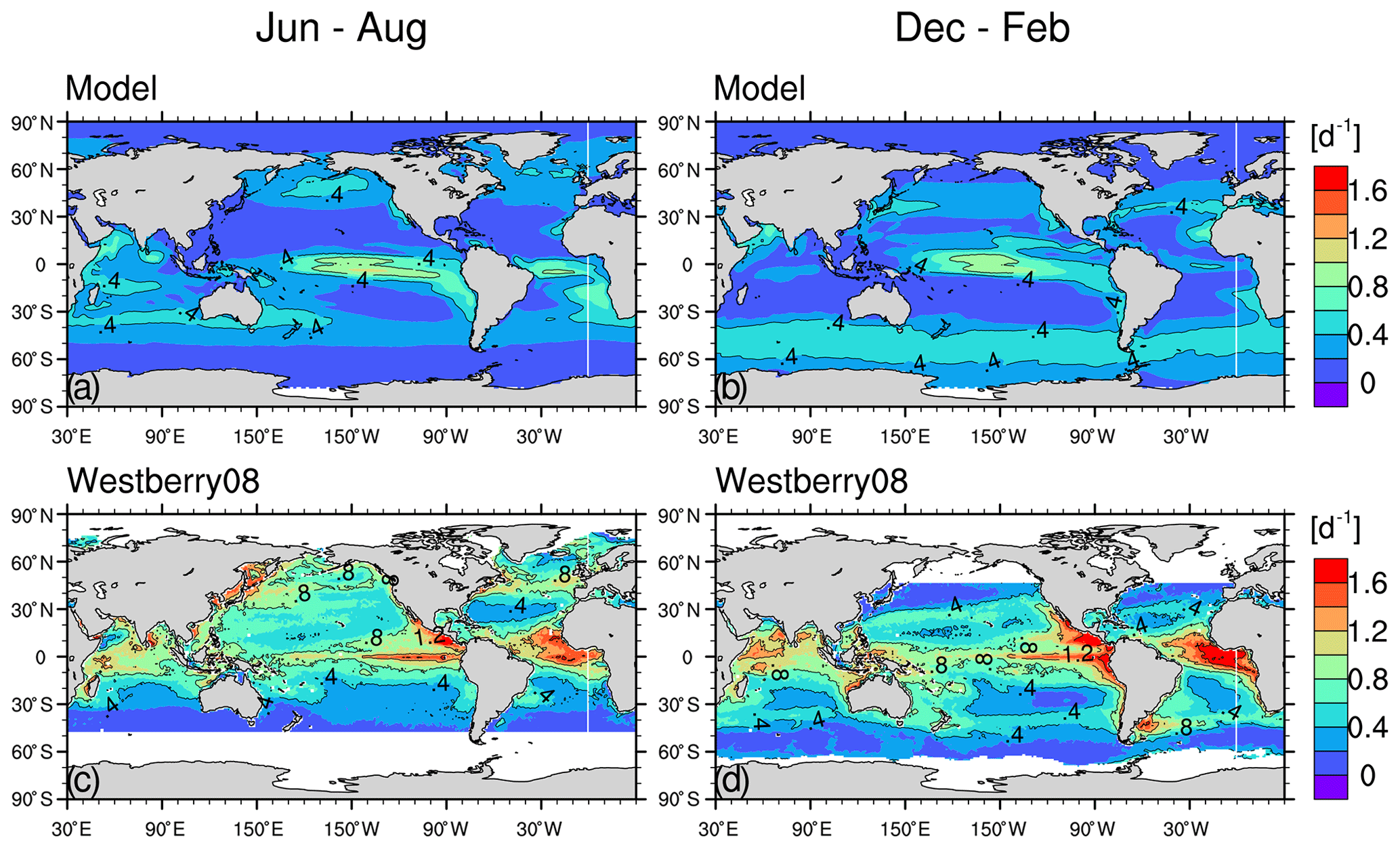
Figure C1The 1999–2004 climatological-mean surface phytoplankton growth rates (d−1) of the model (a, b, for bulk phytoplankton) and of the satellite-based estimates from Westberry et al. (2008) (c, d) for the boreal summer (a, c) and winter (b, d). The growth rate is identical between Hist_Popp and Hist_Laws.
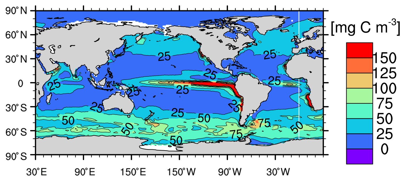
Figure C2The 1999–2004 averaged annual-mean surface phytoplankton biomass (mg C m−3) of the model.
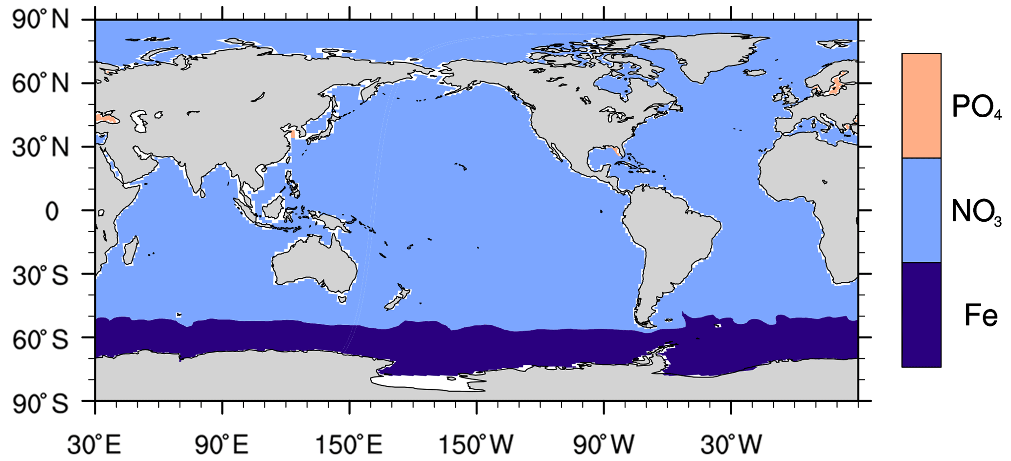
Figure C3Limiting nutrients for primary production in the model.
C2 Additional model–observation comparison for oceanic biogeochemical variables
The model captures the major features of the observed phosphate, DIC, oxygen and nitrate distribution. The biases of the above four variables are shown in Figs. 9b, 10g–i, C4, C5 and C6. We slightly underestimate the global mean phosphate by 0.2 mmol m−3, DIC by 41.3 mmol m−3, oxygen by 15 mmol m−3 and nitrate by 4.7 mmol m−3.

Figure C4(a) DIC biases with respect to observation (GLODAPv1; Key et al., 2004) at the sea surface. (b–d) Zonal-mean DIC biases for the Atlantic, Pacific and Indian Ocean, respectively. Model data are averaged for 1990–1999.
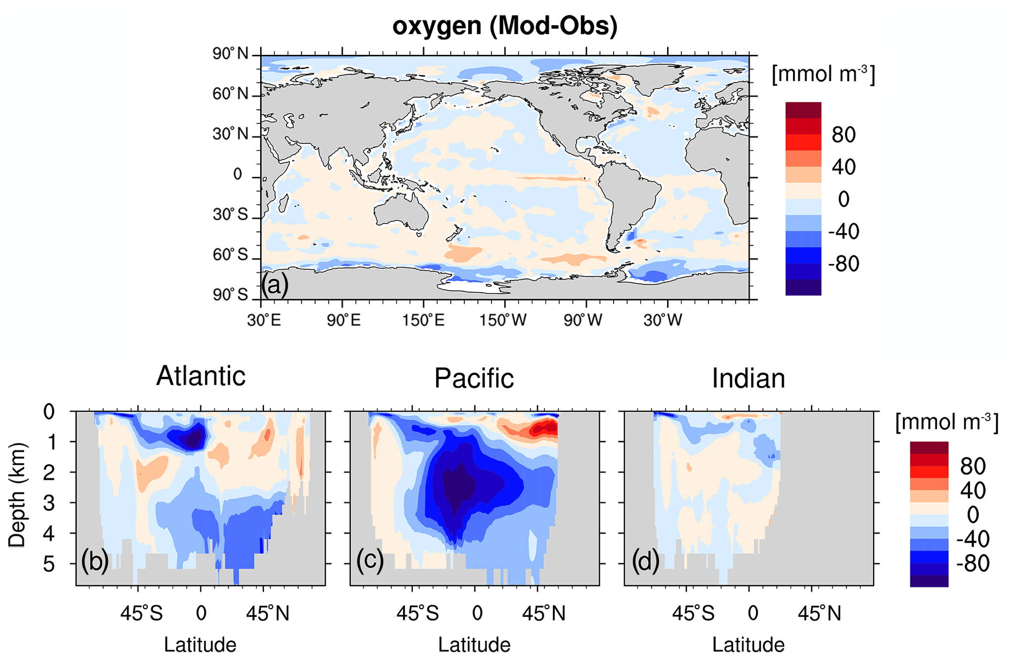
Figure C5As Fig. C4 but for simulated oxygen and observation from WOA13 (Garcia et al., 2013b).
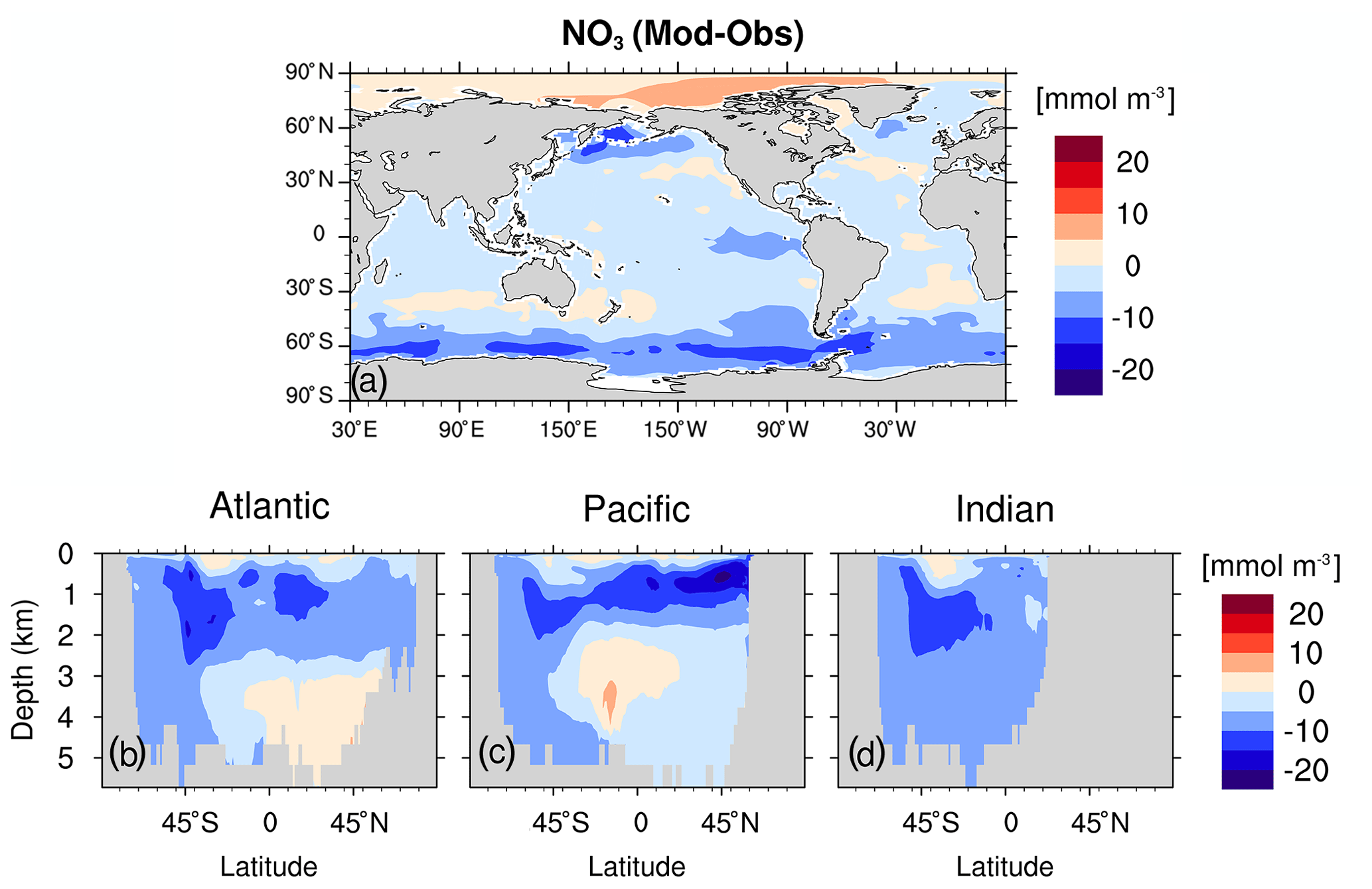
Figure C6As Fig. C4 but for simulated nitrate and observation from WOA13 (Garcia et al., 2013a).

Figure C7The change rate of biological fractionation ϵp from 1960 to 2009.

Figure C8The biological component δ13C at the ocean surface for the model Hist_Popp (a) and observation (b). Panels (c–d) are as panels (a–b) but for the residual component δ13C.
The regenerated component of δ13CDIC, δ13Creg, relates to organic matter remineralisation and calcium carbonate dissolution. We neglect the dissolution of CaCO3 following Sonnerup et al. (1999), who argued that this simplification only results in a small offset (<2 %). δ13Creg is calculated as
with δ13Cpref given in Eq. (15). Note that the calculation of δ13Cpref in Eq. (15) only applies below the 200 m, which is roughly the euphotic zone depth (Eide et al., 2017a).
The temporal change of the regenerated component (Fig. D1a–c) generally shows a much smaller magnitude than δ13C (Fig. 12d–f). Above 1500 m, the δ13C is mainly caused by the change in remineralisation, as is illustrated by the change in AOU (Fig. D1d–f). Below 1500 m, the is generally negative because δ13CPOC decreases by 2.2 ‰ from the pre-industrial period to the 1990s, mainly due to the decline of the biological fractionation factor ϵp under increasing surface CO2(aq) (Fig. C7a).

Figure D1The simulated change in the regenerated component for vertical sections A16 in the Atlantic Ocean (a), P16 in the Pacific Ocean (b) and I8S9N in the Indian Ocean (c). The locations of the vertical sections are shown in Fig. 12. Panels (d–f) are as panels (a–c) but for the change in AOU from pre-industrial times to the 1990s.
E1 Description of the Eide et al. (2017a) approach
To derive the global oceanic 13C Suess effect, Eide et al. (2017a) (hereafter E17) first applied the two-stage back-calculation method developed by Olsen and Ninnemann (2010) to calculate the 13C Suess effect using data from the World Ocean Circulation Experiment sections. The steps and assumptions of this stage are explained below. Next E17 mapped these 13C Suess effect estimates onto a 1 × 1∘ grid with 24 vertical layers and obtained the three-dimension distribution of the 13C Suess effect in the global ocean. For simplicity, hereafter the above procedure is collectively referred to as E17's approach.
E17 first assume that any oceanic CFC-12 signal before 1940 is negligible and the oceanic 13C Suess effect at any time t after 1940, δ13CSE(t−1940), is proportional to CFC-12 partial pressure at time t:
Here the proportionality factor a is time-invariant. δ13CDIC at any time t after year 1940 is decomposed as
The calculation of δ13Cpref is given in Eq. (15) and δ13Creg in Eq. (D1). E17 include two additional terms on the right-hand side of the above equation Δδ13Creg and Δδ13Cpref (see their Eq. 4), which represent any changes not related to the 13C Suess effect, e.g. changes in ocean carbon cycle. We do not explicitly write these two terms as they are set to zero by E17.
Decomposing the left-hand side of Eq. (E2) into a preformed component and a regenerated component gives
Following Gruber et al. (1996), E17 assume a steady-state ocean over the period of interest and set to zero, and this gives
Combining Eqs. (E1) and (E4) yields linear relationship between δ13C and pCFC-12t:
where b contains term δ13C. Thus, the proportionality factor a can be determined with δ13C and pCFC-12t at time t, and δ13CSE(t−1940) can be obtained with Eq. (E1).
To scale δ13CSE(t−1940) to δ13CSE(t−PI) for the full industrial period, the assumption is used that the oceanic δ13CDIC change scales with the atmospheric δ13CO2 change, i.e.:
with
E2 Calculation of SEpref, the oceanic 13C Suess effect estimate using E17's approach and model data
To achieve a result comparable to E17, we select the model data at the geographic locations for which both CFC-12 and δ13CDIC measurements are available. The observational data set of E17 has data from one cruise in the South Atlantic (A13.5) in 2010. We do not include this cruise data because the applied ERA20C forcing, and, thus, our simulations ends in 2009. Here we use the observations compiled by Schmittner et al. (2013) because δ13CDIC in this data set has been quality controlled and is publicly available. Following E17, we use data at the model layers between 200 m and the simulated CFC-12 penetration depth (defined as pCFC-12 = 20 patm (pico-atmosphere); see the thick grey lines in Fig. 14). We take model data of year t=1994. By performing a linear regression (Eq. E5) for five ventilation regions (the North Atlantic, South Atlantic, North Pacific, South Pacific and Indian Ocean) we obtain the regression parameters, hereafter referred to as apref and bpref. Applying Eq. (E6) to the three-dimension model data of pCFC-12 for t=1994, regression slope apref and fatm=1.5 (determined with Eq. E7 for year 1994), we obtain the estimate of the global oceanic 13C Suess effect, SEpref, in year 1994 (Eq. 16).
The regressional relationships between and pCFC-121994 and the regression coefficients apref and bpref are shown in Fig. E2 (the water masses in this figure are defined in Table E1). The coefficient of determination r2, the percentage of the variance in the data explained by the regressional relationship, ranges between 0.33 and 0.66. The strength of these linear relationships is acceptable considering the lowest r2=0.22 in E17.
The regression relationships between δ13Cpref and pCFC-12 in our model (Fig. E2) show some quantitative differences compared to those of E17 (see their Fig. 3). These differences originate from model biases in the distribution and properties of water masses. These mismatches do not affect the analysis and conclusions in Sect. 5. Nevertheless, we briefly discuss their causes for better understanding of the model behaviour.
First, the definitions of several water masses in the model are slightly different from those of E17 (comparing our Table E1 with their Table 2).
Second, our simulated δ13C in the deep and bottom waters (Antarctic Bottom Water, Circumpolar Deep Water, Pacific Deep Water and Indian Deep Water) in the Southern Hemisphere (Fig. E2c and e and Fig. E3c) is higher than that in E17 (see their Fig. 3a, c and e). The possible reasons for this difference are related to mixing and primary production in the Southern Ocean. Here, the simulated deep convection, which primarily occurs in the open ocean rather than the along continental shelf, is too strong in the model. This can be seen by the large mixed layer depth (Fig. B5) and by the CFC-12 bias along selected vertical sections (Fig. B8), which feature persistent positive biases off the Antarctic continental shelf in the Atlantic, Pacific and Indian sectors of the Southern Ocean. Furthermore, the Southern Ocean has a primary production that is too high in the model (about a factor of 1.5 of the satellite-based net primary production estimates from Westberry et al., 2008). The high primary production causes higher surface δ13CDIC than observations (see the South Pacific Ocean in Fig. 8c). Consequently, the simulated preformed component δ13C in the bottom and deep water masses of the Southern Ocean is higher than observed values in E17.
Third, the lowest values of δ13C (<1.4 ‰) are often found in the upwelling regions in the model. This is due to the upward transport of water from the ocean interior that has lower δ13CDIC than observations (Fig. 10e and f).
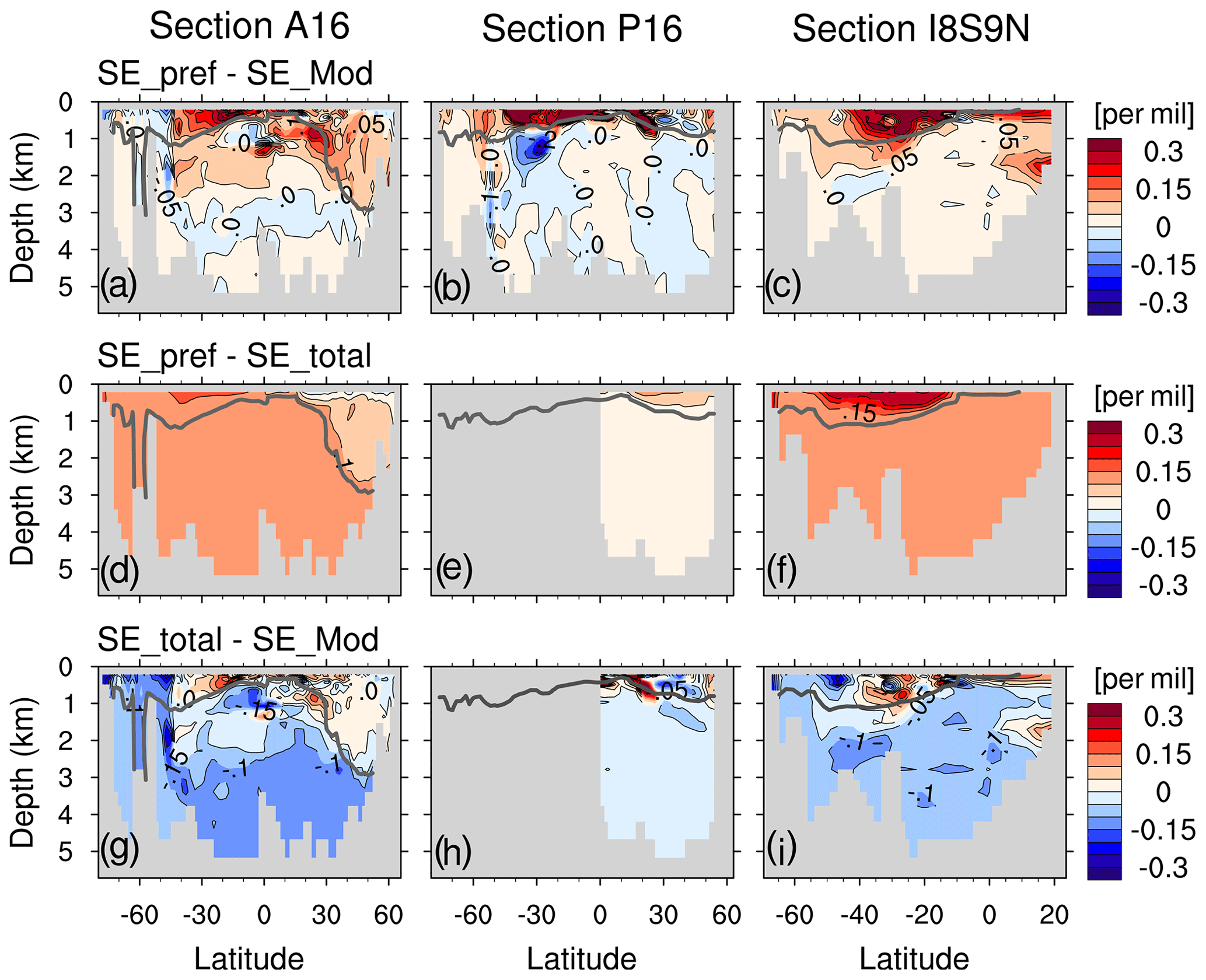
Figure E1The difference (SEpref−SEMod) for the vertical sections A16 in the Atlantic Ocean (a), P16 in the Pacific Ocean (b) and I8S9N in the Indian Ocean (c). Panels (d–f) and (g–i) are as panels (a–c) but for (SEtotal−SEMod) and (SEpref−SEtotal), respectively. The isoline increment is 0.05 ‰. The thick grey line is the pCFC-121994=20 patm isoline, below which SEpref is generally very small (<0.05 ‰).
E3 Linear regression for subregions in the Indian Ocean
We can span regressional relationships for the subtropical gyres of the Indian Ocean and North Pacific Ocean because we use all model levels between 200 m and the pCFC-12 = 20 patm isoline at a given geographical location, and therefore we have more data points than field measurements. In the Indian Ocean, performing linear regression for δ13C and pCFC-121994 in the Subtropical Gyre Water and Sub-Antarctic Mode Water yields regression parameters , and r2=0.49. The more negative compared to regression slope obtained for the whole Indian Ocean suggests an underestimation of the 13C Suess effect. The mean pCFC-12 in the Indian subtropical region at 200 m patm. Following Eq. (E6), we can calculate the mean underestimation for the subtropical Indian Ocean as ‰.
E4 Calculation of SEtotal
To calculate SEtotal we perform a linear regression for the total oceanic 13C Suess effect δ13CSE(1994–1940) and pCFC-121994:
Here the model data are subsampled in the same manner as in Sect. E2. Next, applying a correction for the period prior to 1940 (in analogy to Eq. E6) we obtain the expression of SEtotal in Eq. (19).
The regression relationships in Eq. (E8) and regression coefficients are given in Fig. E3. For the Indian, North Pacific, North Atlantic and South Atlantic Ocean, r2 lies between 0.34 and 0.67, which suggests an acceptable strength of the relationships. In the South Pacific Ocean we find low r2=0.07. This low r2 is a result of the high variability in the change in the regenerated component (Fig. 14h) which corrupts the regression. Therefore we omit the South Pacific in the calculation of SEtotal.
Table E1Water masses and their definitions in the model.

a Water masses are combined together rather than separately defined as in Eide et al. (2017a).
b A different σθ threshold is used here compared to Eide et al. (2017a).
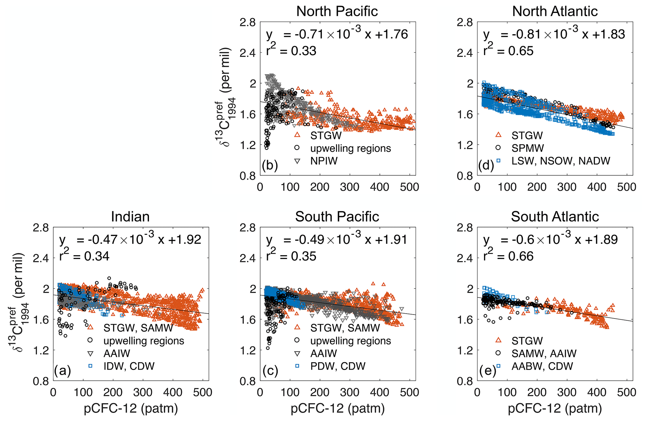
Figure E2Regressional relationships δ13C for the Indian Ocean (a), the North Pacific (b), the South Pacific (c), the North Atlantic (d) and the South Atlantic (e). Different colours and symbols indicate different water masses. The full names, as well as the definitions, of the water masses are listed in Table E1. The regression slopes apref are used to calculate SEpref in Eq. (16). In the Indian Ocean the regression relationship for the Subtropical Gyre Water and Sub-Antarctic Mode Water (red upward triangle in panel a) is . In the North Pacific the regression relationship for the Subtropical Gyre Water (red upward triangle in panel b) is .
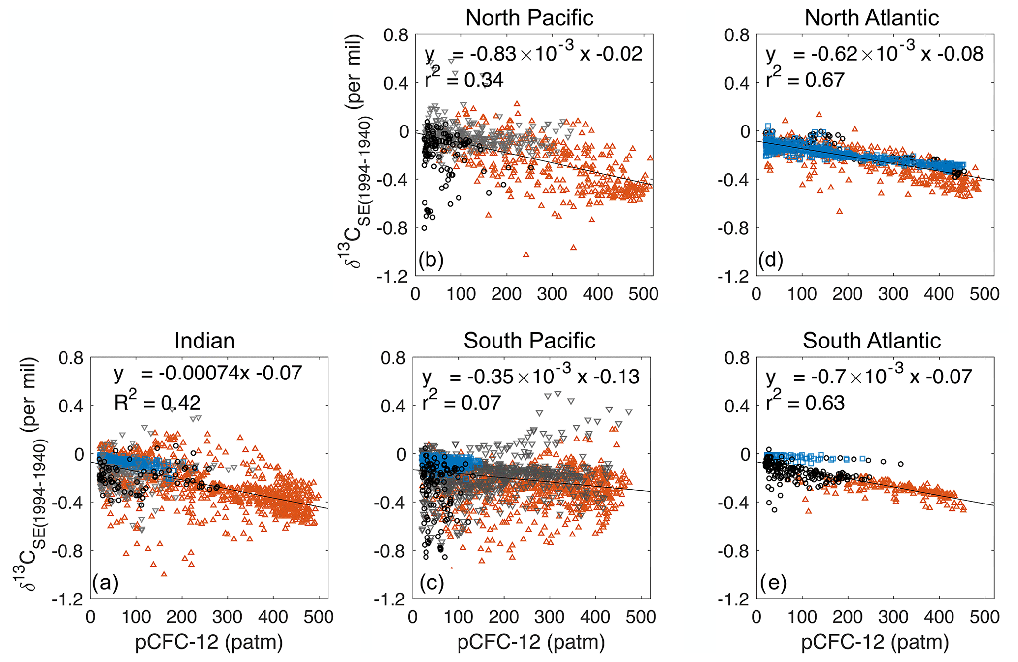
Primary data and code for this study are available from the corresponding author upon request. All observational data used in this study are available from public databases or literature, including the Met Office Hadley Centre EN4 observational data set (https://www.metoffice.gov.uk/hadobs/en4/, last access: 4 March 2020, Good et al., 2013), World Ocean Atlas 2013 (https://www.nodc.noaa.gov/OC5/woa13/pubwoa13.html, last access: 19 February 2015, Garcia et al., 2013a, b), Global Ocean Data Analysis Project version 1 (https://www.ncei.noaa.gov/access/ocean-carbon-data-system/oceans/glodap/, last access: 18 November 2004, Key et al., 2004), net air–sea CO2 flux (now available at https://www.ncei.noaa.gov/access/ocean-carbon-data-system/oceans/SPCO2_1982_2011_ETH_SOM_FFN.html, 19 April 2018, Landschützer et al., 2015), ocean primary production and growth rate (http://sites.science.oregonstate.edu/ocean.productivity/, last access: 13 November 2019, Westberry et al., 2008), δ13CPOC (data provided by Andreas Schmittner in September 2019; this data set was originally compiled by Goericke and Fry, 1994), δ13CDIC (https://andreasschmittner.github.io/publications.html, last access: 8 October 2018, Schmittner et al., 2013), and the oceanic 13C Suess effect estimate (https://doi.pangaea.de/10.1594/PANGAEA.872004, last access: 21 March 2018, Eide et al., 2017c).
BL performed the 13C model development, conducted the simulations and wrote the manuscript. KDS contributed to the model implementation and in setting up the experiments. All authors of the paper critically discussed the analysis of the results and provided valuable input on the presentation of the paper.
The authors declare that they have no conflict of interest.
Publisher’s note: Copernicus Publications remains neutral with regard to jurisdictional claims in published maps and institutional affiliations.
This research contributes to the German paleoclimate modelling initiative PalMod (FKZ: 01LP1505A, 01LP1515C). PalMod is funded by the Bundesministerium für Bildung und Forschung (BMBF), and it is part of the Research for Sustainable Development initiative (FONA). Simulations were performed at the German Climate Computing Center (DKRZ). We thank Irene Stemmler for her valuable input, and we thank Friederike Fröb for the internal review of this paper. We also thank the two reviewers Anne Morée and Pearse Buchanan for their constructive comments.
This research has been supported by the Bundesministerium für Bildung und Forschung (PalMod initiative, FKZ: grant nos. 01LP1505A and 01LP1515C).
The article processing charges for this open-access publication were covered by the Max Planck Society.
This paper was edited by Jack Middelburg and reviewed by Anne Morée and Pearse Buchanan.
Aumont, O., Orr, J. C., Monfray, P., Madec, G., and Maier-Reimer, E.: Nutrient trapping in the equatorial Pacific: The ocean circulation solution, Global Biogeochem. Cy., 13, 351–369, https://doi.org/10.1029/1998GB900012, 1999. a
Bacastow, R. B., Keeling, C. D., Lueker, T. J., Wahlen, M., and Mook, W. G.: The 13C Suess Effect in the world surface oceans and its implications for oceanic uptake of CO2: Analysis of observations at Bermuda, Global Biogeochem. Cy., 10, 335–346, https://doi.org/10.1029/96GB00192, 1996. a, b
Böhm, F., Joachimski, M., Lehnert, H., Morgenroth, G., Kretschmer, W., Vacelet, J., and Dullo, W.-C.: Carbon isotope records from extant Caribbean and South Pacific sponges: Evolution of δ13C in surface water DIC, Earth Planet. Sc. Lett., 139, 291–303, https://doi.org/10.1016/0012-821X(96)00006-4, 1996. a
Böhm, F., Joachimski, M. M., Dullo, W.-C., Eisenhauer, A., Lehnert, H., Reitner, J., and Wörheide, G.: Oxygen isotope fractionation in marine aragonite of coralline sponges, Geochim. Cosmochim. Ac., 64, 1695–1703, https://doi.org/10.1016/S0016-7037(99)00408-1, 2000. a
Boyd, P. W., Watson, A. J., Law, C. S., Abraham, E. R., Trull, T., Murdoch, R., Bakker, D. C. E., Bowie, A. R., Buesseler, K. O., Chang, H., Charette, M., Croot, P., Downing, K., Frew, R., Gall, M., Hadfield, M., Hall, J., Harvey, M., Jameson, G., LaRoche, J., Liddicoat, M., Ling, R., Maldonado, M. T., McKay, R. M., Nodder, S., Pickmere, S., Pridmore, R., Rintoul, S., Safi, K., Sutton, P., Strzepek, R., Tanneberger, K., Turner, S., Waite, A., and Zeldis, J.: A mesoscale phytoplankton bloom in the polar Southern Ocean stimulated by iron fertilization, Nature, 407, 695–702, https://doi.org/10.1038/35037500, 2000. a
Broecker, W. S. and Maier-Reimer, E.: The influence of air and sea exchange on the carbon isotope distribution in the sea, Global Biogeochem. Cy., 6, 315–320, https://doi.org/10.1029/92GB01672, 1992. a
Broecker, W. S. and Peng, T. H.: Gas exchange rates between air and sea, Tellus A, 26, 21–35, https://doi.org/10.3402/tellusa.v26i1-2.9733, 1974. a
Broecker, W. S. and Peng, T. H.: Evaluation of the 13C constraint on the uptake of fossil fuel CO2 by the ocean, Global Biogeochem. Cy., 7, 619–626, https://doi.org/10.1029/93GB01445, 1993. a, b, c
Buchanan, P. J., Matear, R. J., Chase, Z., Phipps, S. J., and Bindoff, N. L.: Ocean carbon and nitrogen isotopes in CSIRO Mk3L-COAL version 1.0: a tool for palaeoceanographic research, Geosci. Model Dev., 12, 1491–1523, https://doi.org/10.5194/gmd-12-1491-2019, 2019. a, b
Bullister, J. L.: Atmospheric Histories (1765–2015) for CFC-11, CFC-12, CFC-113, CCl4, SF6 and N2O (NCEI Accession 0164584), NOAA National Centers for Environmental Information, https://doi.org/10.3334/CDIAC/otg.CFC_ATM_Hist_2015, 2017. a, b
Chavez, F. P., Buck, K. R., Service, S. K., Newton, J., and Barber, R. T.: Phytoplankton variability in the central and eastern tropical Pacific, Deep-Sea Res. Pt. II, 43, 835–870, https://doi.org/10.1016/0967-0645(96)00028-8, 1996. a
Craig, H.: Isotopic standards for carbon and oxygen and correction factors for mass-spectrometric analysis of carbon dioxide, Geochim. Cosmochim. Ac., 12, 133–149, https://doi.org/10.1016/0016-7037(57)90024-8, 1957. a
Cravatte, S., Kessler, W. S., and Marin, F.: Intermediate Zonal Jets in the Tropical Pacific Ocean Observed by Argo Floats, J. Phys. Oceanogr., 42, 1475–1485, https://doi.org/10.1175/JPO-D-11-0206.1, 2012. a
Cunningham, S. A., Alderson, S. G., King, B. A., and Brandon, M. A.: Transport and variability of the Antarctic Circumpolar Current in Drake Passage, J. Geophys. Res.-Oceans, 108, 8084, https://doi.org/10.1029/2001JC001147, 2003. a
Curry, W. B. and Oppo, D. W.: Glacial water mass geometry and the distribution of δ13C of ΣCO2 in the western Atlantic Ocean, Paleoceanography, 20, PA1017, https://doi.org/10.1029/2004PA001021, 2005. a
de Boyer Montégut, C., Madec, G., Fischer, A. S., Lazar, A., and Iudicone, D.: Mixed layer depth over the global ocean: An examination of profile data and a profile-based climatology, J. Geophys. Res.-Oceans, 109, C12003, https://doi.org/10.1029/2004JC002378, 2004. a
Degens, E., Behrendt, M., Gotthardt, B., and Reppmann, E.: Metabolic fractionation of carbon isotopes in marine plankton – II. Data on samples collected off the coasts of Peru and Ecuador, Deep-Sea Res., 15, 11–20, https://doi.org/10.1016/0011-7471(68)90025-9, 1968. a
Dentith, J. E., Ivanovic, R. F., Gregoire, L. J., Tindall, J. C., and Robinson, L. F.: Simulating stable carbon isotopes in the ocean component of the FAMOUS general circulation model with MOSES1 (XOAVI), Geosci. Model Dev., 13, 3529–3552, https://doi.org/10.5194/gmd-13-3529-2020, 2020. a, b, c
Dietze, H. and Loeptien, U.: Revisiting “nutrient trapping” in global coupled biogeochemical ocean circulation models, Global Biogeochem. Cy., 27, 265–284, https://doi.org/10.1002/gbc.20029, 2013. a, b
Donohue, K. A., Tracey, K. L., Watts, D. R., Chidichimo, M. P., and Chereskin, T. K.: Mean Antarctic Circumpolar Current transport measured in Drake Passage, Geophys. Res. Lett., 43, 11760–11767, https://doi.org/10.1002/2016GL070319, 2016. a
Dutay, J.-C., Bullister, J. L., Doney, S. C., Orr, J. C., Najjar, R., Caldeira, K., Campin, J.-M., Drange, H., Follows, M., Gao, Y., Gruber, N., Hecht, M. W., Ishida, A., Joos, F., Lindsay, K., Madec, G., Maier-Reimer, E., Marshall, J. C., Matear, R. J., Monfray, P., Mouchet, A., Plattner, G.-K., Sarmiento, J., Schlitzer, R., Slater, R., Totterdell, I. J., Weirig, M.-F., Yamanaka, Y., and Yool, A.: Evaluation of ocean model ventilation with CFC-11: comparison of 13 global ocean models, Ocean Model., 4, 89–120, https://doi.org/10.1016/S1463-5003(01)00013-0, 2002. a
Eide, M., Olsen, A., Ninnemann, U. S., and Eldevik, T.: A global estimate of the full oceanic 13C Suess effect since the preindustrial, Global Biogeochem. Cy., 31, 492–514, https://doi.org/10.1002/2016GB005472, 2017a. a, b, c, d, e, f, g, h, i, j, k, l, m, n, o, p, q, r, s, t, u, v, w, x, y, z, aa, ab
Eide, M., Olsen, A., Ninnemann, U. S., and Johannessen, T.: A global ocean climatology of preindustrial and modern ocean δ13C, Global Biogeochem. Cy., 31, 515–534, https://doi.org/10.1002/2016GB005473, 2017b. a, b, c, d
Eide, M., Olsen, A., Ninnemann, U. S., Eldevik, T., and Johannessen, T.: Climatological distributions of δ13C of dissolved inorganic carbon in the global oceans, Geophysical Institute, University of Bergen and Bjerknes Centre for Climate Research, PANGAEA [data set], https://doi.org/10.1594/PANGAEA.872004, 2017c. a
Francois, R., Altabet, M. A., Goericke, R., McCorkle, D. C., Brunet, C., and Poisson, A.: Changes in the δ13C of surface water particulate organic matter across the subtropical convergence in the SW Indian Ocean, Global Biogeochem. Cy., 7, 627–644, https://doi.org/10.1029/93GB01277, 1993. a, b, c, d
Gammon, R. H., Cline, J., and Wisegarver, D.: Chlorofluoromethanes in the northeast Pacific Ocean: Measured vertical distributions and application as transient tracers of upper ocean mixing, J. Geophys. Res.-Oceans, 87, 9441–9454, https://doi.org/10.1029/JC087iC12p09441, 1982. a
Garcia, H. E., Locarnini, R. A., Boyer, T. P., Antonov, J. I., Baranova, O. K., Zweng, M. M., Reagan, J. R., and Johnson, D. R.: World Ocean Atlas 2013, Volume 4: Dissolved Inorganic Nutrients (phosphate, nitrate, silicate), Tech. Rep., 25, NOAA Atlas NESDIS 76, available at: https://www.nodc.noaa.gov/OC5/woa13/pubwoa13.html (last access: 15 December 2019), 2013a. a, b, c, d
Garcia, H. E., Locarnini, R. A., Boyer, T. P., Antonov, J. I., Baranova, O. K., Zweng, M. M., Reagan, J. R., and Johnson, D. R.: World Ocean Atlas 2013, Volume 3: Dissolved Oxygen, Apparent Oxygen Utilization, and Oxygen Saturation, Tech. Rep., 27, NOAA Atlas NESDIS 75, available at: https://www.nodc.noaa.gov/OC5/woa13/pubwoa13.html (last access: 15 December 2019), 2013b. a, b, c
Goericke, R. and Fry, B.: Variations of marine plankton δ13C with latitude, temperature, and dissolved CO2 in the world Ocean, Global Biogeochem. Cy., 8, 85–90, https://doi.org/10.1029/93gb03272, 1994. a, b, c, d, e
Good, S. A., Martin, M. J., and Rayner, N. A.: EN4: Quality controlled ocean temperature and salinity profiles and monthly objective analyses with uncertainty estimates, J. Geophys. Res.-Oceans, 118, 6704–6716, https://doi.org/10.1002/2013JC009067, 2013 (data available at: https://www.metoffice.gov.uk/hadobs/en4/, last access: 4 March 2020). a, b, c, d
Gruber, N., Sarmiento, J. L., and Stocker, T. F.: An improved method for detecting anthropogenic CO2 in the oceans, Global Biogeochem. Cy., 10, 809–837, https://doi.org/10.1029/96GB01608, 1996. a
Gruber, N., Keeling, C. D., Bacastow, R. B., Guenther, P. R., Lueker, T. J., Wahlen, M., Meijer, H. A. J., Mook, W. G., and Stocker, T. F.: Spatiotemporal patterns of carbon-13 in the global surface oceans and the oceanic Suess effect, Global Biogeochem. Cy., 13, 307–335, https://doi.org/10.1029/1999GB900019, 1999. a
Hansman, R. L. and Sessions, A. L.: Measuring the in situ carbon isotopic composition of distinct marine plankton populations sorted by flow cytometry, Limnol. Oceanogr.-Meth., 14, 87–99, https://doi.org/10.1002/lom3.10073, 2016. a
Heinze, C. and Maier-Reimer, E.: The Hamburg Oceanic CarbonCycle Circulation Model Version “HAMOCC2s” for long time integrations, Tech. Rep., 20, Max Planck Institute for Meteorology, Hamburg, Germany, 1999. a
Heinze, C., Maier-Reimer, E., Winguth, A. M. E., and Archer, D.: A global oceanic sediment model for long-term climate studies, Global Biogeochem. Cy., 13, 221–250, https://doi.org/10.1029/98GB02812, 1999. a
Hofmann, M., Wolf-Gladrow, D. A., Takahashi, T., Sutherland, S. C., Six, K. D., and Maier-Reimer, E.: Stable carbon isotope distribution of particulate organic matter in the ocean: a model study, Mar. Chem., 72, 131–150, https://doi.org/10.1016/S0304-4203(00)00078-5, 2000. a
Holte, J., Talley, L. D., Gilson, J., and Roemmich, D.: An Argo mixed layer climatology and database, Geophys. Res. Lett., 44, 5618–5626, https://doi.org/10.1002/2017GL073426, 2017. a
Ilyina, T., Six, K. D., Segschneider, J., Maier-Reimer, E., Li, H., and Núñez-Riboni, I.: Global ocean biogeochemistry model HAMOCC: Model architecture and performance as component of the MPI-Earth system model in different CMIP5 experimental realizations, J. Adv. Model. Earth Sy., 5, 287–315, https://doi.org/10.1029/2012MS000178, 2013. a
Jahn, A., Lindsay, K., Giraud, X., Gruber, N., Otto-Bliesner, B. L., Liu, Z., and Brady, E. C.: Carbon isotopes in the ocean model of the Community Earth System Model (CESM1), Geosci. Model Dev., 8, 2419–2434, https://doi.org/10.5194/gmd-8-2419-2015, 2015. a, b
Jones, C. D., Arora, V., Friedlingstein, P., Bopp, L., Brovkin, V., Dunne, J., Graven, H., Hoffman, F., Ilyina, T., John, J. G., Jung, M., Kawamiya, M., Koven, C., Pongratz, J., Raddatz, T., Randerson, J. T., and Zaehle, S.: C4MIP – The Coupled Climate–Carbon Cycle Model Intercomparison Project: experimental protocol for CMIP6, Geosci. Model Dev., 9, 2853–2880, https://doi.org/10.5194/gmd-9-2853-2016, 2016. a, b, c
Jungclaus, J. H., Fischer, N., Haak, H., Lohmann, K., Marotzke, J., Matei, D., Mikolajewicz, U., Notz, D., and Storch, J. S.: Characteristics of the ocean simulations in the Max Planck Institute Ocean Model (MPIOM) the ocean component of the MPI-Earth system model, J. Adv. Model. Earth Sy., 5, 422–446, https://doi.org/10.1002/jame.20023, 2013. a, b
Keeling, C. D.: The Suess effect: 13Carbon-14Carbon interrelations, Environment International, 2, 229–300, https://doi.org/10.1016/0160-4120(79)90005-9, 1979. a
Keller, K. and Morel, F. M. M.: A model of carbon isotopic fractionation and active carbon uptake in phytoplankton, Mar. Ecol. Prog. Ser., 182, 295–298, https://doi.org/10.3354/meps182295, 1999. a
Key, R. M., Kozyr, A., Sabine, C. L., Lee, K., Wanninkhof, R., Bullister, J. L., Feely, R. A., Millero, F. J., Mordy, C., and Peng, T.-H.: A global ocean carbon climatology: Results from Global Data Analysis Project (GLODAP), Global Biogeochem. Cy., 18, GB4031, https://doi.org/10.1029/2004GB002247, 2004 (data available at: https://www.ncei.noaa.gov/access/ocean-carbon-data-system/oceans/glodap/, last access: 18 November 2004). a, b, c, d
Kriest, I. and Oschlies, A.: On the treatment of particulate organic matter sinking in large-scale models of marine biogeochemical cycles, Biogeosciences, 5, 55–72, https://doi.org/10.5194/bg-5-55-2008, 2008. a
Landschützer, P., Gruber, N., and Bakker, D.: A 30 years observation-based global monthly gridded sea surface pCO2 product from 1982 through 2011, Carbon Dioxide Information Analysis Center, Oak Ridge National Laboratory, US Department of Energy, Oak Ridge, Tennessee, now available at: https://www.ncei.noaa.gov/access/ocean-carbon-data-system/oceans/SPCO2_1982_2011_ETH_SOM_FFN.html (last access: 19 April 2018), 2015. a, b
Latif, M., Claussen, M., Schulz, M., and Brücher, T.: Comprehensive Earth system models of the last glacial cycle, Eos: Earth & Space Science News, 97, https://doi.org/10.1029/2016EO059587, 2016. a, b
Laws, E. A., Popp, B. N., Bidigare, R. R., Kennicutt, M. C., and Macko, S. A.: Dependence of phytoplankton carbon isotopic composition on growth rate and [CO2]aq: Theoretical considerations and experimental results, Geochim. Cosmochim. Ac., 59, 1131–1138, https://doi.org/10.1016/0016-7037(95)00030-4, 1995. a, b, c, d, e, f, g
Letelier, R., Dore, J., Winn, C., and Karl, D.: Seasonal and interannual variations in photosynthetic carbon assimilation at Station, Deep-Sea Res. Pt. II, 43, 467–490, https://doi.org/10.1016/0967-0645(96)00006-9, 1996. a
Liang, X., Spall, M., and Wunsch, C.: Global Ocean Vertical Velocity From a Dynamically Consistent Ocean State Estimate, J. Geophys. Res.-Oceans, 122, 8208–8224, https://doi.org/10.1002/2017JC012985, 2017. a, b
Lide, D. R.: CRC Handbook of Chemistry and Physics, CRC Press, Boca Raton, Florida, 2002. a
Lynch-Stieglitz, J., Stocker, T. F., Broecker, W. S., and Fairbanks, R. G.: The influence of air-sea exchange on the isotopic composition of oceanic carbon: observations and modelling, Global Biogeochem. Cy., 9, 653–665, https://doi.org/10.1029/95GB02574, 1995. a, b, c
Maier-Reimer, E.: Geochemical cycles in an ocean general circulation model. Preindustrial tracer distributions, Global Biogeochem. Cy., 7, 645–677, https://doi.org/10.1029/93GB01355, 1993. a
Marañón, E.: Phytoplankton growth rates in the Atlantic subtropical gyres, Limnol. Oceanogr., 50, 299–310, https://doi.org/10.4319/lo.2005.50.1.0299, 2005. a
Martin, J. H., Knauer, G. A., Karl, D. M., and Broenkow, W. W.: VERTEX: carbon cycling in the northeast Pacific, Deep-Sea Res., 34, 267–285, https://doi.org/10.1016/0198-0149(87)90086-0, 1987. a
Mauritsen, T., Bader, J., Becker, T., Behrens, J., Bittner, M., Brokopf, R., Brovkin, V., Claussen, M., Crueger, T., Esch, M., Fast, I., Fiedler, S., Fläschner, D., Gayler, V., Giorgetta, M., Goll, D., Haak, H., Hagemann, S., Hedemann, C., Hohenegger, C., Ilyina, T., Jahns, T., Jimenéz-de-la-Cuesta, D., Jungclaus, J., Kleinen, T., Kloster, S., Kracher, D., Kinne, S., Kleberg, D., Lasslop, G., Kornblueh, L., Marotzke, J., Matei, D., Meraner, K., Mikolajewicz, U., Modali, K., Möbis, B., Müller, W., Nabel, J., Nam, C., Notz, D., Nyawira, S., Paulsen, H., Peters, K., Pincus, R., Pohlmann, H., Pongratz, J., Popp, M., Raddatz, T., Rast, S., Redler, R., Reick, C., Rohrschneider, T., Schemann, V., Schmidt, H., Schnur, R., Schulzweida, U., Six, K., Stein, L., Stemmler, I., Stevens, B., von Storch, J., Tian, F., Voigt, A., de Vrese, P., Wieners, K.-H., Wilkenskjeld, S., Winkler, A., and Roeckner, E.: Developments in the MPI-M Earth System Model version 1.2 (MPI-ESM1.2) and Its Response to Increasing CO2, J. Adv. Model. Earth Sy., 11, 998–1038, https://doi.org/10.1029/2018MS001400, 2019. a, b, c, d
Meinshausen, M., Vogel, E., Nauels, A., Lorbacher, K., Meinshausen, N., Etheridge, D. M., Fraser, P. J., Montzka, S. A., Rayner, P. J., Trudinger, C. M., Krummel, P. B., Beyerle, U., Canadell, J. G., Daniel, J. S., Enting, I. G., Law, R. M., Lunder, C. R., O'Doherty, S., Prinn, R. G., Reimann, S., Rubino, M., Velders, G. J. M., Vollmer, M. K., Wang, R. H. J., and Weiss, R.: Historical greenhouse gas concentrations for climate modelling (CMIP6), Geosci. Model Dev., 10, 2057–2116, https://doi.org/10.5194/gmd-10-2057-2017, 2017. a, b
Meredith, M. P., Woodworth, P. L., Chereskin, T. K., Marshall, D. P., Allison, L. C., Bigg, G. R., Donohue, K., Heywood, K. J., Hughes, C. W., Hibbert, A., Hogg, A. M., Johnson, H. L., Jullion, L., King, B. A., Leach, H., Lenn, Y.-D., Morales Maqueda, M. A., Munday, D. R., Naveira Garabato, A. C., Provost, C., Sallée, J.-B., and Sprintall, J.: Sustained monitoring of the Southern Ocean at Drake Passage: Past achievements and future priorities, Rev. Geophys., 49, RG4005, https://doi.org/10.1029/2010RG000348, 2011. a
Moore, C. M., Mills, M. M., Arrigo, K. R., Berman-Frank, I., Bopp, L., Boyd, P. W., Galbraith, E. D., Geider, R. J., Guieu, C., Jaccard, S. L., Jickells, T. D., La Roche, J., Lenton, T. M., Mahowald, N. M., Marañón, E., Marinov, I., Moore, J. K., Nakatsuka, T., Oschlies, A., Saito, M. A., Thingstad, T. F., Tsuda, A., and Ulloa, O.: Processes and patterns of oceanic nutrient limitation, Nat. Geosci., 6, 701–710, https://doi.org/10.1038/ngeo1765, 2013. a, b
Msadek, R., Johns, W. E., Yeager, S. G., Danabasoglu, G., Del-worth, T. L., and Rosati, A.: The Atlantic meridional heat transport at 26.5∘ N and its relationship with the MOC in the RAPID array and the GFDL and NCAR coupled models, J. Climate, 26, 4335–4356, https://doi.org/10.1175/JCLI-D-12-00081.1, 2013. a
Notz, D., Haumann, F. A., Haak, H., Jungclaus, J. H., and Marotzke, J.: Arctic sea-ice evolution as modeled by Max Planck Institute for Meteorology's Earth system model, J. Adv. Model. Earth Sy., 5, 173–194, https://doi.org/10.1002/jame.20016, 2013. a
Nowlin Jr., W. D. and Klinck, J. M.: The physics of the Antarctic Circumpolar Current, Rev. Geophys., 24, 469–491, https://doi.org/10.1029/RG024i003p00469, 1986. a
O'Leary, M. H.: Carbon Isotopes in Photosynthesis, BioScience, 38, 328–336, https://doi.org/10.2307/1310735, 1988. a
Olsen, A. and Ninnemann, U.: Large δ13C Gradients in the Preindustrial North Atlantic Revealed, Science, 330, 658–659, https://doi.org/10.1126/science.1193769, 2010. a
Olsen, A., Key, R. M., van Heuven, S., Lauvset, S. K., Velo, A., Lin, X., Schirnick, C., Kozyr, A., Tanhua, T., Hoppema, M., Jutterström, S., Steinfeldt, R., Jeansson, E., Ishii, M., Pérez, F. F., and Suzuki, T.: The Global Ocean Data Analysis Project version 2 (GLODAPv2) – an internally consistent data product for the world ocean, Earth Syst. Sci. Data, 8, 297–323, https://doi.org/10.5194/essd-8-297-2016, 2016. a
O'Neill, C. M., Hogg, A. McC., Ellwood, M. J., Eggins, S. M., and Opdyke, B. N.: The [simple carbon project] model v1.0, Geosci. Model Dev., 12, 1541–1572, https://doi.org/10.5194/gmd-12-1541-2019, 2019. a
Orr, J. C., Najjar, R. G., Aumont, O., Bopp, L., Bullister, J. L., Danabasoglu, G., Doney, S. C., Dunne, J. P., Dutay, J.-C., Graven, H., Griffies, S. M., John, J. G., Joos, F., Levin, I., Lindsay, K., Matear, R. J., McKinley, G. A., Mouchet, A., Oschlies, A., Romanou, A., Schlitzer, R., Tagliabue, A., Tanhua, T., and Yool, A.: Biogeochemical protocols and diagnostics for the CMIP6 Ocean Model Intercomparison Project (OMIP), Geosci. Model Dev., 10, 2169–2199, https://doi.org/10.5194/gmd-10-2169-2017, 2017. a, b, c
Paulsen, H., Ilyina, T., Six, K. D., and Stemmler, I.: Incorporating a prognostic representation of marine nitrogen fixers into the global ocean biogeochemical model HAMOCC, J. Adv. Model. Earth Sy., 9, 438–464, https://doi.org/10.1002/2016MS000737, 2017. a, b
Peterson, C. D., Lisiecki, L. E., and Stern, J. V.: Deglacial whole-ocean δ13C change estimated from 480 benthic foraminiferal records, Paleoceanography, 29, 549–563, https://doi.org/10.1002/2013PA002552, 2014. a
Poli, P., Hersbach, H., Dee, D. P., Berrisford, P., Simmons, A. J., Vitart, F., Laloyaux, P., Tan, D. G. H., Peubey, C., Thépaut, J.-N., Trémolet, Y., Hólm, E. V., Bonavita, M., Isaksen, L., and Fisher, M.: ERA-20C: An Atmospheric Reanalysis of the Twentieth Century, J. Climate, 29, 4083–4097, https://doi.org/10.1175/JCLI-D-15-0556.1, 2016. a
Popp, B. N., Takigiku, R., Hayes, J. M., Louda, J. W., and Baker, E. W.: The post-Paleozoic chronology and mechanism of 13C depletion in primary marine organic matter, Am. J. Sci., 289, 436–454, https://doi.org/10.2475/ajs.289.4.436, 1989. a, b, c, d, e, f
Popp, B. N., Laws, E. A., Bidigare, R. R., Dore, J. E., Hanson, K. L., and Wakeham, S. G.: Effect of Phytoplankton Cell Geometry on Carbon Isotopic Fractionation, Geochim. Cosmochim. Ac., 62, 69–77, https://doi.org/10.1016/S0016-7037(97)00333-5, 1998. a
Quay, P., Sonnerup, R., Westby, T., Stutsman, J., and McNichol, A.: Changes in the of dissolved inorganic carbon in the ocean as a tracer of anthropogenic CO2 uptake, Global Biogeochem. Cy., 17, 1004, https://doi.org/10.1029/2001GB001817, 2003. a, b
Rau, G. H., Riebesell, U., and Wolf-Gladrow, D.: A model of photosynthetic 13C fractionation by marine phytoplankton based on diffusive molecular CO2 uptake, Mar. Ecol. Prog. Ser., 133, 275–285, https://doi.org/10.3354/meps133275, 1996. a
Sabine, C. L., Feely, R. A., Gruber, N., Key, R. M., Lee, K., Bullister, J. L., Wanninkhof, R., Wong, C. S., Wallace, D. W. R., Tilbrook, B., Millero, F. J., Peng, T.-H., Kozyr, A., Ono, T., and Rios, A. F.: The Oceanic Sink for Anthropogenic CO2, Science, 305, 367–371, https://doi.org/10.1126/science.1097403, 2004. a
Schmittner, A., Gruber, N., Mix, A. C., Key, R. M., Tagliabue, A., and Westberry, T. K.: Biology and air–sea gas exchange controls on the distribution of carbon isotope ratios (δ13C) in the ocean, Biogeosciences, 10, 5793–5816, https://doi.org/10.5194/bg-10-5793-2013, 2013 (data available at: https://andreasschmittner.github.io/publications.html, last access: 8 October 2018). a, b, c, d, e, f, g, h, i, j, k, l, m, n, o, p, q, r, s, t, u
Schmittner, A., Bostock, H. C., Cartapanis, O., Curry, W. B., Filipsson, H. L., Galbraith, E. D., Gottschalk, J., Herguera, J. C., Hoogakker, B., Jaccard, S. L., Lisiecki, L. E., Lund, D. C., Martínez-Méndez, G., Lynch-Stieglitz, J., Mackensen, A., Michel, E., Mix, A. C., Oppo, D. W., Peterson, C. D., Repschläger, J., Sikes, E. L., Spero, H. J., and Waelbroeck, C.: Calibration of the carbon isotope composition (δ13C) of benthic foraminifera, Paleoceanography, 32, 512–530, https://doi.org/10.1002/2016PA003072, 2017. a
Silsbe, G. M., Behrenfeld, M. J., Halsey, K. H., Milligan, A. J., and Westberry, T. K.: The CAFE model: A net production model for global ocean phytoplankton, Global Biogeochem. Cy., 30, 1756–1777, https://doi.org/10.1002/2016GB005521, 2016. a
Six, K. D. and Maier-Reimer, E.: Effects of plankton dynamics on seasonal carbon fluxes in an ocean general circulation model, Global Biogeochem. Cy., 10, 559–583, https://doi.org/10.1029/96GB02561, 1996. a
Smeed, D., McCarthy, G., Rayner, D., Moat, B. I., Johns, W. E., Baringer, M. O., and Meinen, C. S.: Atlantic meridional overturning circulation observed by the RAPID-MOCHA-WBTS (RAPID-Meridional Overturning Circulation and Heatflux Array-Western Boundary Time Series) array at 26N from 2004 to 2017, British Oceanographic Data Centre, Natural Environment Research Council, https://doi.org/10.5285/5acfd143-1104-7b58-e053-6c86abc0d94b, 2017. a
Sonnerup, R. E., Quay, P. D., McNichol, A. P., Bullister, J. L., Westby, T. A., and Anderson, H. L.: Reconstructing the oceanic 13C Suess Effect, Global Biogeochem. Cy., 13, 857–872, https://doi.org/10.1029/1999GB900027, 1999. a, b
Sonnerup, R. E., Mcnichol, A. P., Quay, P. D., Gammon, R. H., Bullister, J. L., Sabine, C. L., and Slater, R. D.: Anthropogenic δ13C changes in the North Pacific Ocean reconstructed using a multiparameter mixing approach (MIX), Tellus B, 59, 303–317, https://doi.org/10.1111/j.1600-0889.2007.00250.x, 2007. a
Swart, P. K., Thorrold, S., Rosenheim, B., Eisenhauer, A., Harrison, C. G. A., Grammer, M., and Latkoczy, C.: Intra-annual variation in the stable oxygen and carbon and trace element composition of sclerosponges, Paleoceanography, 17, 1045, https://doi.org/10.1029/2000PA000622, 2002. a
Swart, P. K., Greer, L., Rosenheim, B. E., Moses, C. S., Waite, A. J., Winter, A., Dodge, R. E., and Helmle, K.: The 13C Suess effect in scleractinian corals mirror changes in the anthropogenic CO2 inventory of the surface oceans, Geophys. Res. Lett., 37, L05604, https://doi.org/10.1029/2009GL041397, 2010. a
Tagliabue, A. and Bopp, L.: Towards understanding global variability in ocean carbon-13, Global Biogeochem. Cy., 22, GB1025, https://doi.org/10.1029/2007GB003037, 2008. a
Takahashi, T., Broecker, W. S., and Langer, S.: Redfield ratio based on chemical data from isopycnal surfaces, J. Geophys. Res.-Oceans, 90, 6907–6924, https://doi.org/10.1029/JC090iC04p06907, 1985. a
Takahashi, T., Sutherland, S., Chipman, D., Goddard, J., Ho, C., Newberger, T., Sweeney, C., and Munro, D.: Climatological distributions of pH, pCO2, total CO2, alkalinity, and CaCO3 saturation in the global surface ocean, and temporal changes at selected locations, Mar. Chem., 164, 95–125, https://doi.org/10.1016/j.marchem.2014.06.004, 2014. a
Tjiputra, J. F., Schwinger, J., Bentsen, M., Morée, A. L., Gao, S., Bethke, I., Heinze, C., Goris, N., Gupta, A., He, Y.-C., Olivié, D., Seland, Ø., and Schulz, M.: Ocean biogeochemistry in the Norwegian Earth System Model version 2 (NorESM2), Geosci. Model Dev., 13, 2393–2431, https://doi.org/10.5194/gmd-13-2393-2020, 2020. a, b, c, d, e, f
Tuerena, R. E., Ganeshram, R. S., Humphreys, M. P., Browning, T. J., Bouman, H., and Piotrowski, A. P.: Isotopic fractionation of carbon during uptake by phytoplankton across the South Atlantic subtropical convergence, Biogeosciences, 16, 3621–3635, https://doi.org/10.5194/bg-16-3621-2019, 2019. a
Turner, J. V.: Kinetic fractionation of carbon-13 during calcium carbonate precipitation, Geochim. Cosmochim. Ac., 46, 1183–1191, https://doi.org/10.1016/0016-7037(82)90004-7, 1982. a
Wanninkhof, R.: Relationship between wind speed and gas exchange over the ocean revisited, Limnol. Oceanogr.-Meth., 12, 351–362, https://doi.org/10.4319/lom.2014.12.351, 2014. a
Weisberg, R. H. and Qiao, L.: Equatorial Upwelling in the Central Pacific Estimated from Moored Velocity Profilers, J. Phys. Oceanogr., 30, 105–124, https://doi.org/10.1175/1520-0485(2000)030<0105:EUITCP>2.0.CO;2, 2000. a
Weiss, R. F.: Carbon dioxide in water and seawater: the solubility of a non-ideal gas, Mar. Chem., 2, 203–215, https://doi.org/10.1016/0304-4203(74)90015-2, 1974. a
Westberry, T., Behrenfeld, M. J., Siegel, D. A., and Boss, E.: Carbon-based primary productivity modeling with vertically resolved photoacclimation, Global Biogeochem. Cy., 22, GB2024, https://doi.org/10.1029/2007GB003078, 2008 (data availabe at: http://sites.science.oregonstate.edu/ocean.productivity/, last access: 13 November 2019). a, b, c, d, e, f
Wörheide, G.: The reef cave dwelling ultraconservative coralline demospongeAstrosclera willeyana Lister 1900 from the Indo-Pacific, Facies, 38, 1–88, https://doi.org/10.1007/BF02537358, 1998. a
Young, J. N., Bruggeman, J., Rickaby, R. E. M., Erez, J., and Conte, M.: Evidence for changes in carbon isotopic fractionation by phytoplankton between 1960 and 2010, Global Biogeochem. Cy., 27, 505–515, https://doi.org/10.1002/gbc.20045, 2013. a, b, c
Zeebe, R. E. and Wolf-Gladrow, D. A.: CO2 in Seawater: Equilibrium, Kinetics, Isotopes, Elsevier Oceanography Series, Amsterdam, 2001. a, b
Zhang, J., Quay, P., and Wilbur, D.: Carbon isotope fractionation during gas-water exchange and dissolution of CO2, Geochim. Cosmochim. Ac., 59, 107–114, https://doi.org/10.1016/0016-7037(95)91550-D, 1995. a, b
- Abstract
- Introduction
- Model description
- Model results and observations in the late 20th century
- Evaluation of the simulated oceanic 13C Suess effect
- Potential sources of uncertainties in an observation-based global oceanic 13C Suess effect estimate
- Summary and conclusions
- Appendix A: Governing factors for the water-column DI13C inventory changes
- Appendix B: Model–observation comparison of ocean physics
- Appendix C: Model–observation comparison of ocean biogeochemistry
- Appendix D: The regenerated component of δ13CDIC
- Appendix E: Applying the Eide et al. (2017a) approach to the model data
- Code and data availability
- Author contributions
- Competing interests
- Disclaimer
- Acknowledgements
- Financial support
- Review statement
- References