the Creative Commons Attribution 4.0 License.
the Creative Commons Attribution 4.0 License.
 | 21 Feb 2022
A seamless ensemble-based reconstruction of surface ocean pCO2 and air–sea CO2 fluxes over the global coastal and open oceans
Thi Tuyet Trang Chau
Marion Gehlen
Frédéric Chevallier
We have estimated global air–sea CO2 fluxes (fgCO2) from the open ocean to coastal seas. Fluxes and associated uncertainty are computed from an ensemble-based reconstruction of CO2 sea surface partial pressure (pCO2) maps trained with gridded data from the Surface Ocean CO2 Atlas v2020 database. The ensemble mean (which is the best estimate provided by the approach) fits independent data well, and a broad agreement between the spatial distribution of model–data differences and the ensemble standard deviation (which is our model uncertainty estimate) is seen. Ensemble-based uncertainty estimates are denoted by ±1σ. The space–time-varying uncertainty fields identify oceanic regions where improvements in data reconstruction and extensions of the observational network are needed. Poor reconstructions of pCO2 are primarily found over the coasts and/or in regions with sparse observations, while fgCO2 estimates with the largest uncertainty are observed over the open Southern Ocean (44∘ S southward), the subpolar regions, the Indian Ocean gyre, and upwelling systems.
Our estimate of the global net sink for the period 1985–2019 is 1.643±0.125 PgC yr−1 including 0.150±0.010 PgC yr−1 for the coastal net sink. Among the ocean basins, the Subtropical Pacific (18–49∘ N) and the Subpolar Atlantic (49–76∘ N) appear to be the strongest CO2 sinks for the open ocean and the coastal ocean, respectively. Based on mean flux density per unit area, the most intense CO2 drawdown is, however, observed over the Arctic (76∘ N poleward) followed by the Subpolar Atlantic and Subtropical Pacific for both open-ocean and coastal sectors. Reconstruction results also show significant changes in the global annual integral of all open- and coastal-ocean CO2 fluxes with a growth rate of PgC yr−2 and a temporal standard deviation of 0.526±0.022 PgC yr−1 over the 35-year period. The link between the large interannual to multi-year variations of the global net sink and the El Niño–Southern Oscillation climate variability is reconfirmed.
- Article
(4511 KB) - Full-text XML
-
Supplement
(4005 KB) - BibTeX
- EndNote


Since the onset of the industrial era, humankind has profoundly modified the global carbon (C) cycle. The use of fossil fuels, cement production, and land use change added 700±75 PgC (best estimate ±1σ) to the atmosphere between 1750 and 2019 (Friedlingstein et al., 2020). An estimated 285±5 PgC of this excess C stayed there; the remainder was taken up by the ocean (170±20 PgC) and the land biosphere (230 ± 60 PgC). While the fraction of total CO2 emissions sequestered by the ocean has remained rather stable (22 %–25 %) over the past 6 decades (Friedlingstein et al., 2020), the global ocean sink has varied significantly at interannual timescales (Rödenbeck et al., 2015). Global ocean biogeochemical models (GOBMs) are used within the framework of the annual assessment of the global carbon budget (Friedlingstein et al., 2020) to annually re-estimate the means of and variations in CO2 sinks and sources over the global ocean and major basins. However, these recent model-based estimates need to be benchmarked against observation-based estimates in order to better understand the global carbon budget as well as its yearly re-distribution in the biosphere (Hauck et al., 2020).
In situ measurements of sea surface fugacity of CO2 collected by an international coordinated effort of the ocean observation community and combined into the Surface Ocean CO2 Atlas (SOCAT, https://www.socat.info/, last access: 16 June 2020; Bakker et al., 2016) provide an observational constraint on the assessment of the surface ocean partial pressure of CO2 (pCO2) and the ocean C sinks and sources. Despite an increasing number of observations since the 1990s, data density remains uneven in space and time. While, for instance, data coverage is sparse over the southern basins of the Atlantic and Pacific oceans, observations are seasonally biased towards the summers at high latitudes (Landschützer et al., 2014; Denvil-Sommer et al., 2019; Gregor et al., 2019).
Various data-based approaches have been proposed to infer gridded maps of surface ocean pCO2 from the sparse set of observation-based data. They have been successful in obtaining similarly low misfits between the reconstructed and evaluation data and reasonable estimates of air–sea CO2 fluxes (see Rödenbeck et al., 2015; Gregor et al., 2019; Friedlingstein et al., 2020) although model design and implementation are quite different (e.g. the proportion of SOCAT data used in model fitting and evaluation). Aside from data reconstruction built on a single model mapping pCO2 data with machine learning, classical regression, or mixed-layer schemes (e.g. Rödenbeck et al., 2013; Landschützer et al., 2016; Iida et al., 2021), ensemble-based approaches have recently emerged but with their own concepts and objectives. For example, Denvil-Sommer et al. (2019) designed a two-step reconstruction of pCO2 climatologies and anomalies based on five neural network models and selected the one that reproduced the pCO2 field with the smallest model–data misfit. Gregor et al. (2019) and Gregor and Gruber (2021) introduced machine-learning ensembles with 6 to 16 different two-step clustering–regression models mapping surface pCO2 and suggest that the use of their ensemble mean is better than each member estimate. In a broader context, Rödenbeck et al. (2015) presented an intercomparison of 14 mapping methods targeting the identification of common or distinguishable features of different products in long-term mean, regional, and temporal variations. Hauck et al. (2020) and Friedlingstein et al. (2020) also synthesized pCO2 mapping products and took an ensemble of their observation-based estimates of air–sea CO2 fluxes as a benchmark to compare with the one derived from ocean biogeochemical models.
Despite positive conclusions overall, statistical data reconstructions are still subject to further improvements. In Rödenbeck et al. (2015), Hauck et al. (2020), Bushinsky et al. (2019), and Denvil-Sommer et al. (2021), the authors explain that substantial extensions of surface ocean observational network systems are essential to better determine pCO2 and fluxes at finer scales and reduce mapping uncertainties. So far mapping uncertainties have been estimated by using misfits between the model outputs and SOCAT data (e.g. the root-mean-square deviation, RMSD). By construction, such uncertainty estimates are restricted to oceanic regions and periods when observations are available (Rödenbeck et al., 2015; Lebehot et al., 2019; Gregor et al., 2019), and the uncertainty quantification of an averaged pCO2 or an integrated flux over the space and time of interest is with low confidence due to sparse data density. Also, most of the aforementioned mapping methods target pCO2 data and estimate air–sea fluxes solely over the open ocean, with the coastal data excluded or not fully qualified. In Laruelle et al. (2014), the authors present spatial distributions of air–sea flux density and estimates of the total coastal C sink inferred from spatial integration methods on coastal SOCAT data. Laruelle et al. (2017) adapted the two-step neural network approach described in Landschützer et al. (2016) to the coastal-ocean pCO2. The coastal and open-ocean products were combined into a single reconstruction to yield a global monthly climatology of pCO2 presented in Landschützer et al. (2020). Notwithstanding these advances, a global reconstruction and its uncertainty assessment of monthly varying coastal surface ocean pCO2 and air–sea fluxes are still missing.
In this work, we propose a new inference strategy for reconstructing the monthly pCO2 fields and the contemporary air–sea fluxes over the period 1985–2019 with a spatial resolution of 1∘ × 1∘. It is based on a Monte Carlo approach, an ensemble of 100 neural network models mapping sub-samples drawn from the monthly gridded SOCATv2020 data and available data of predictors. This ensemble approach was developed at the Laboratoire des Sciences du Climat et de l'Environnement (LSCE) as both an extension of and an improvement on the first version (LSCE-FFNN-v1; Denvil-Sommer et al., 2019). In the following sections, we first present the ensemble of neural networks designed with the aims of leaving aside the issue of discrete boundaries in the existing two-step clustering–regressions (see further discussion in Gregor and Gruber, 2021) and reducing the mapping uncertainties induced by the two-step reconstruction of the pCO2 fields (Denvil-Sommer et al., 2019) or by an ensemble-based reconstruction with a small ensemble size. In addition, each feed-forward neural network (FFNN) model follows a leave-p-out cross-validation approach, i.e. the exclusion of p gridded SOCAT data of the reconstructed month itself in model training and validation. This allows us to reduce model over-fitting and to leave many more independent data for model evaluation than in the previous studies. The mean and standard deviation computed from the ensemble of 100 model outputs are defined as estimates of the mean state and uncertainty in the carbon fields. As one of the novel key findings of this study compared to the existing ones, we compute and analyse the estimates of pCO2 and air–sea fluxes, model errors, and model uncertainties for different timescales (e.g. monthly, yearly, and multi-decadal) and spatial scales (e.g. grid cells, sub-basins, and the global ocean). We then suggest the use of an indicator map built on the space–time-varying uncertainty fields instead of model–data misfits for identifying regions that should be prioritized in future observational programmes and model development in order to improve data reconstruction. Last but not least, the model best estimates of and uncertainty in pCO2 and air–sea fluxes are analysed seamlessly over the open ocean to the coastal zone. Potential drivers of the spatio-temporal distribution and the magnitude of open-ocean and coastal CO2 fluxes are discussed with the aim to better identify underlying processes and to detect potential focus regions for further studies on the evolution of oceanic CO2 sources and sinks.
2.1 General formulation
The air–sea flux density (molC m−2 yr−1) is calculated here by the standard bulk equation
where k is the gas transfer velocity computed as a function of the 10 m ERA5 wind speed (Hersbach et al., 2020) following Wanninkhof (2014) and its coefficient is scaled to match a global mean transfer velocity of 16.5 cm h−1 (Naegler, 2009). L is the temperature-dependent solubility of CO2 (Weiss, 1974), fice and are the sea-ice fraction and the atmospheric CO2 partial pressure, respectively. In Eq. (1), a positive (negative) flux indicates oceanic CO2 uptake (release). Details and references for the source of these variables are given in Table S1 in the Supplement, except for pCO2, which is described in the following section.
2.2 An ensemble-based approach for the reconstruction of sea surface pCO2 and air–sea CO2 fluxes
The sea surface partial pressure of CO2 in Eq. (1) is estimated monthly over each point of the global ocean by analysing sparse in situ measurements of CO2 fugacity, gathered and gridded at a monthly and 1∘ resolution in the 2020 release of the Surface Ocean CO2 Atlas (SOCATv2020, https://www.socat.info/, last access: 16 June 2020). SOCATv2020 covers the period 1985–2019. First, monthly gridded pCO2 data were converted from SOCATv2020 CO2 fugacity (Körtzinger, 1999). We then regressed these pCO2 values against a set of predictors with non-linear functions, i.e. feed-forward neural network (FFNN) models. As illustrated in Fig. 1, our predictors are biological, chemical, and physical variables commonly associated with the variations in pCO2 (e.g. Landschützer et al., 2013; Denvil-Sommer et al., 2019; Gregor et al., 2019): sea surface height (SSH), sea surface temperature (SST), sea surface salinity (SSS), mixed-layer depth (MLD), chlorophyll a (chl a), and atmospheric CO2 mole fraction (xCO2). A pCO2 climatology (Takahashi et al., 2009) and the geographical coordinates (latitude and longitude) were also added to the predictors. Table S1 details the data source. All data were reprocessed and co-located at the same SOCAT resolution following Landschützer et al. (2016) and Denvil-Sommer et al. (2019). For instance, chl a was set approximately to 0 mg m−3 over the Arctic and the Southern Ocean winter when no data were available. In the case of data being unavailable before 1998, climatologies based on all available data were used as predictors. Exceptionally, predictors for SSH before 1993 were climatologies plus a linear trend in order to retain the overall response to the global warming. The MLD before 1992 was taken as the average MLD between 1992 and 1997.

Figure 1Illustration of a feed-forward neural network (FFNN) model mapping monthly gridded SOCAT data and feature variables (Table S1) co-located at a spatial resolution of 1∘ × 1∘.
An ensemble of 100 FFNN models was used to reconstruct monthly pCO2 fields with a 1∘ × 1∘ resolution over the global surface ocean during the years 1985–2019. This ensemble approach was developed at the Laboratoire des Sciences du Climat et de l'Environnement (LSCE) as both an extension of and an improvement on the first version (LSCE-FFNN-v1; Denvil-Sommer et al., 2019). Our model outputs are part of the Copernicus Marine Environment Monitoring Service (CMEMS). Throughout the paper, it is hence referred to as CMEMS-LSCE-FFNN.
To reconstruct the pCO2 fields over the global ocean for each target month over the 1985–2019 period, all the available SOCAT data and the co-located predictors have been collected for the month before and the month after the target month. We randomly extracted two-thirds of each one of these datasets to make training datasets for the FFNN models, leaving the remaining third to be corresponding test datasets. The FFNN models were then trained for each target month. Moreover, the exclusion of the reconstructed month itself in the training and test datasets follows a leave-p-out cross-validation approach, where p is the number of gridded SOCAT data in the target month. This approach allows us to reduce model over-fitting, as well as to assess the quality of the reconstruction against SOCAT data that are fully independent from the training phase.
The random extraction and the FFNN training were repeated 100 times so that 100 versions of the monthly FFNN models have been obtained. Note that our ensemble approach belongs to the classes of bootstrapping and Monte Carlo methods in statistics. Theoretically, the number of samples or the ensemble size must be substantially large to obtain a convergence. However, it was demonstrated in the literature (e.g. Goodhue et al., 2012; Efron et al., 2015) that with an ensemble size of 50 the model estimation is likely stable and with an ensemble size over 100 the improvement in standard errors between model outputs and evaluation data is negligible. Figure S2 in the Supplement shows an illustration of the reconstruction skill with respect to the ensemble size S. For each ensemble of S model outputs of pCO2 (), the root-mean-square deviation (RMSD) is computed between the ensemble mean (our best model estimate) and SOCAT data over the period 1985–2019. As seen in this figure, the reconstruction starts to stabilize with S=50. In this study, we have exploited a large but realistic amount of computing resources to run an ensemble of S=100 neural network models. Equation (1) was then applied to the ensembles of FFNN outputs of pCO2 in order to obtain ensembles of monthly global fgCO2 fields.
2.3 Coastal and regional division
The reconstructed pCO2 fields and air–sea CO2 fluxes are analysed over the global ocean, at particular locations, and in 11 oceanic sub-basins used by the Regional Carbon Cycle Assessment and Processes Tier 1 (RECCAP1; Canadell et al., 2011) and previous studies (Schuster et al., 2013; Sarma et al., 2013; Ishii et al., 2014; Lenton et al., 2013; Wanninkhof et al., 2013; Landschützer et al., 2014). In order to distinguish the coastal from the open ocean, we use the coastal mask from the MARgins and CATchments Segmentation (MARCATS; Laruelle et al., 2013) interpolated on the 1∘ × 1∘ SOCAT grid. Details of the regional (open and coastal) division are given in Table 1 and Fig. 2.
Table 1Indication of 11 RECCAP1 regions (Fig. 2). Only the total area with respect to the maximum coverage of the reconstructed data is accounted for in each region.
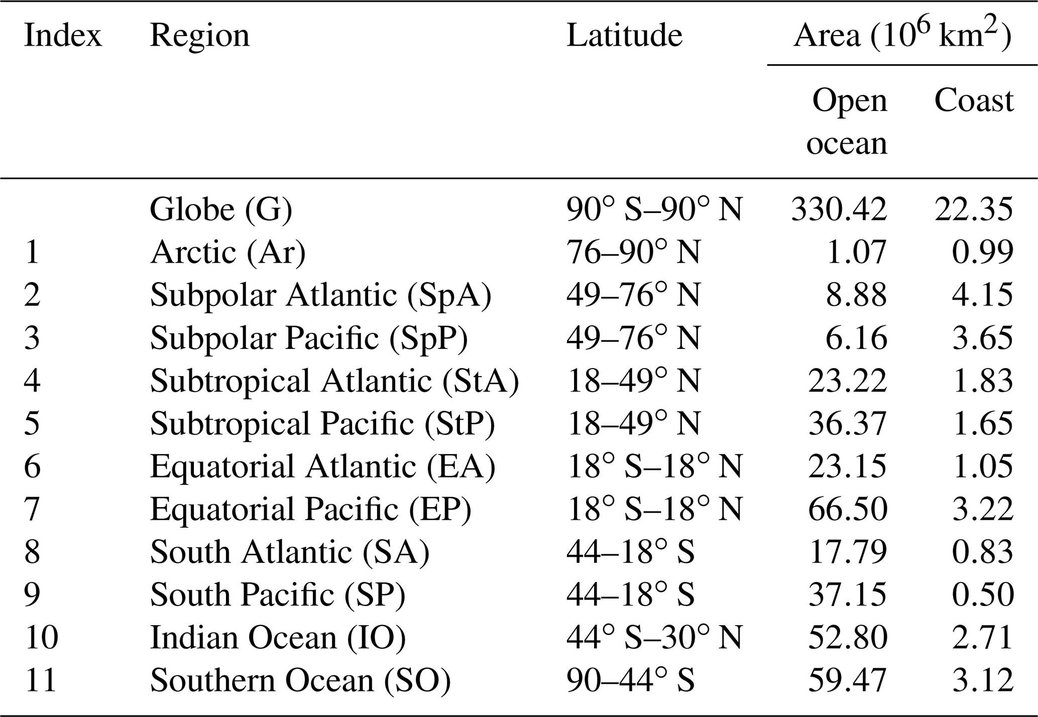
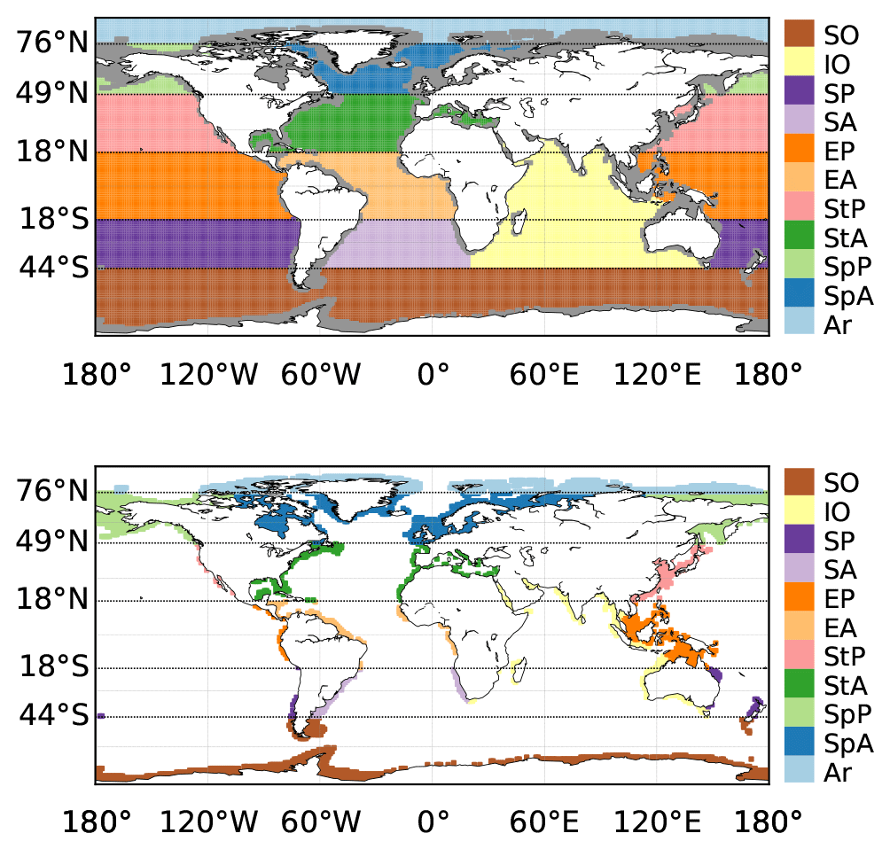
Figure 2Map of RECCAP1 regions (Regional Carbon Cycle Assessment and Processes; Canadell et al., 2011) and MARCATS (MARgins and CATchments Segmentation) coastal mask (Laruelle et al., 2013) co-located on the 1∘ × 1∘ SOCAT grid.
With the above definitions, the coastal regions encompass 6.33 % of a total maximum ocean area of 352.77×10⁶ km2. The computation of these numbers was based on the maximum data coverage of the CMEMS-LSCE-FFNN reconstruction taking into account the variable monthly sea-ice fraction. The number of monthly gridded SOCATv2020 data used in the reconstruction of pCO2 is reported in Table S2 for each region, with 301 449 in total and 10.36 % of the data available over the predefined coastal regions.
2.4 Statistics
The mean (μ) and standard deviation (σ) of the 100-member ensembles of pCO2 and fgCO2 are chosen as their best estimate and the associated uncertainty, respectively. Unless stated otherwise, a model best estimate and its uncertainty computed at each desired space–time resolution are denoted by μensemble±σensemble, where
and is one of the 100 members of the reconstructed pCO2 fields. Similar definitions are applied for fgCO2. The units of air–sea flux estimates are molC m−2 yr−1 for a flux density, and this is converted to PgC yr−1 for an integral over a region or the global ocean.
Model robustness of the reconstructed pCO2 fields is evaluated on the gridded SOCAT data and in situ observations (Sutton et al., 2019). The evaluation data are denoted as in the following formulas. Standard statistics include the coefficient of determination (r2); misfit mean (model bias) and misfit standard deviation,
and the root-mean-square deviation (RMSD),
where and N is a number of evaluation data. All these scores are computed for different coastal and open regions from the scale of grid cells to the global scale.
Generally, RMSD measures the reconstruction skill in terms of the mean distance between model estimates and evaluation data, while r2 measures the proportion of data variation predicted by the model. Compared to other metrics such as mean absolute bias and r2, the RMSD takes another role, an outlier detector, which gives larger weights to high model–data misfits. Note that r2, μmisfit, σmisfit, and RMSD reflect the model performance with respect to evaluation data, while σensemble measures the stability of the model best estimate μensemble. Nevertheless, these different statistics should consistently reflect the skill of the model reconstruction, e.g. depending on the density and distribution of data sampling.
In the next section, both the temporal and the spatial distributions of gridded SOCAT data and in situ observations, model–data errors, model best estimates, and uncertainties are shown. An intensive analysis is presented for both the open-ocean and the coastal zones. We then interpret key factors leading to a good or poor reconstruction of surface pCO2 and fgCO2, e.g. SOCAT data density and distribution, model design and resolution, regional to local characteristics of pCO2 and fgCO2, and their potential driving mechanisms.
3.1 Evaluation
To verify the robustness of the mapping method, we first evaluate the goodness of fit of reconstructed pCO2 against the independent SOCAT data from the leave-p-out cross-validation set (see Sect. 2.2).
Empirical cumulative distribution functions (CDFs) and frequency histograms drawn from these data are compared in Fig. 3a and b. While a frequency histogram in Fig. 3a shows the number of gridded SOCAT pCO2 data distributed for each bin, the one in Fig. 3b (grey) reflects how the pCO2 values in observational grid boxes are distributed within their bounds. The probability–probability (P–P) plot of Fig. 3b (blue curve) measures the fit in the distributions of the reconstruction and SOCAT data. The same presentation is used in Fig. 3c and d for the misfit standard deviation σmisfit and the ensemble standard deviation σensemble (see their definitions in Eqs. 2 and 3 and their values in Fig. S3c and g).
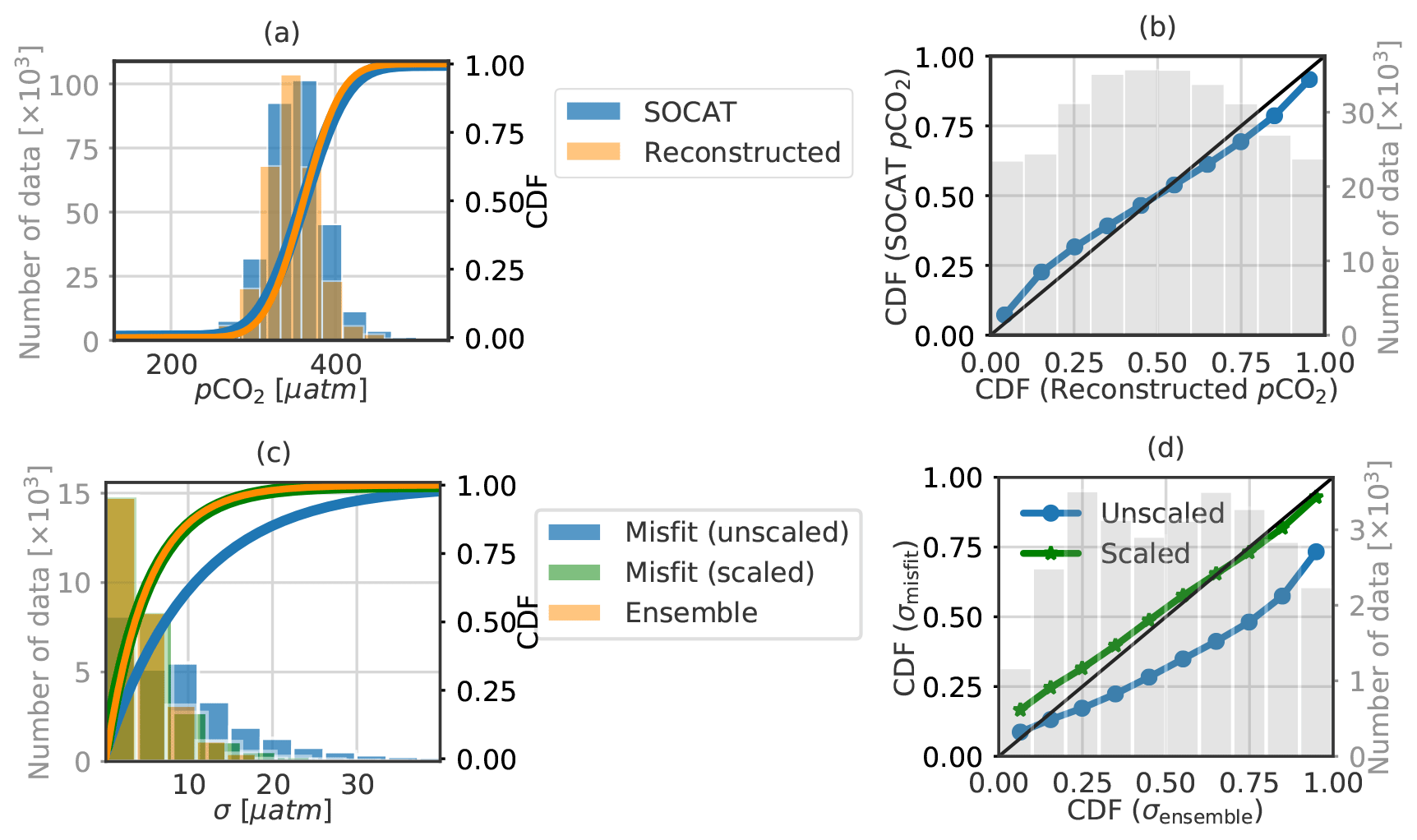
Figure 3Comparison between empirical cumulative distribution functions (CDFs) of (a, b) SOCATv2020 data and the reconstructed pCO2 field and (c, d) model–data misfit standard deviation (σmisfit) and model uncertainty (σensemble), as seen in Fig. S3. In (c) and (d), the distribution of σmisfit values scaled with a factor of 2 is plotted. A histogram with the axis in grey of the four subplots displays the number of gridded data distributed in each bin; the bins with fewer than 200 data for (a) and 20 data for (c) have been excluded. In (b) and (d), the bisector is shown in black.
The reconstructed pCO2 field matches SOCAT data well: both are normally distributed with the same mean of 361.3 µatm (Fig. 3a), and a high agreement for all percentiles (Fig. 3b) is seen. The slight under- or overestimation at high and low percentiles implies that the model is slightly biased towards the mean value, as is expected when predictor variables do not fully explain predictand variables in the training dataset. This reduced variability is also reflected in the difference between the data standard deviation based on SOCAT pCO2 (41.79 µatm) and the one based on CMEMS-LSCE-FFNN (36.30 µatm).
Displayed in Fig. 3c, both misfit standard deviation (σmisfit) and model uncertainty (σensemble) empirically follow the exponential distribution. σmisfit is much higher than σensemble as the CDF and frequency histogram of the former (blue) show heavier tails than those of the latter (orange), which brings the P–P curve below the bisector in Fig. 3d. When dividing the misfit standard deviation values shown in Fig. S3c by 2, σmisfit (green) shares a similar distribution to σensemble (orange). A natural explanation for this 2-fold tuning factor would point to a simple lack of spread of the ensemble, either because the FFNN ensemble would be too small or because the uncertainty in the predictors (not accounted for here in the ensemble) would be significant. The SOCAT CO2 fugacity data are sampled at an uneven space–time resolution (e.g. the sampling frequency varies between one read per minute to one per hour). Gridded data correspond to the average of measurements collected within a 1∘ × 1∘ box and in a month over the entire cell area. Variability in the sampling time and location of cruises and instruments induces temporal sampling bias (e.g. towards some days in a month and/or the summer months at high latitudes) and latitude and longitude offsets from the cell centre (e.g. with an average of 0.34∘ ± 0.14∘ as reported in Sabine et al., 2013), which are not taken into account.
Assume that
-
such practical imperfection presents a systematic error in each measurement from the true data with an overall standard deviation of σobservation and
-
systematic errors between SOCAT data and the reconstructed data equal those between the true data and the reconstructed data.
As observation errors are independent from the random errors induced by the ensemble approach in each grid cell (further to the implementation of the leave-p-out cross-validation in model training; see Sect. 2.2), σmisfit in Eq. (3) can be interpreted as
where varies in space and time and is larger near shelves (see the observation variability in Fig. S1b and c).
The interpretation of the magnitude of mismatch is therefore not straightforward, but we note that the spatial distribution of model errors and uncertainty estimates over the global ocean (Fig. 5) consistently identifies the spatial distribution of the model skill. This asset is prioritized in our preliminary study and further analysed in the next sections. The 2-fold factor used for the illustration in Fig. 3 has not been kept for the following results.
3.1.1 Global ocean
At the global scale, the model fits the data with a mean bias close to zero, an RMSD of 20.48 µatm, and a coefficient of determination (r2) of 0.76. The temporal fluctuation of the spatial mean of the model–data mean difference over the global ocean is displayed in Fig. 4a along with the number of available gridded data. The time series of the yearly bias (black curve) starts with a large positive value (7.47±1.60 µatm) in the year 1985 (∼740 gridded data). The bias drops during the following years and fluctuates around zero from 1994 onwards (the number of grid boxes containing SOCAT observations per year is generally larger than 5000). In general, the magnitudes of the yearly model bias and model spread are correlated with the number of observation-based data, which has increased greatly since the 1990s. The importance of sustained data coverage is emphasized by Fig. S4. It illustrates the fact that large model–data mismatches are frequently associated with the interruption of voluntary observing ship (VOS) lines and thus with the tracking of CO2 fugacity over large regions. The larger bias computed prior to the 1990s (Fig. 4a) might intuitively lead to the conclusion that model outputs are less reliable than those in the later periods. However, this global mean score is influenced by the number and distribution of data, and consequently the increased data density does not fully explain the reconstruction skill. For instance, even with a higher number of observation-based data than that in the pre-1990s, the years 2001 and 2007 stand out with strong negative biases ( and µatm, respectively). While such a comparison between the global bias and the number of data highlights the lack of a simple relationship between the number of data and the skill of the mapping method, the ensemble spread (dark grey area) of model errors, representing the spread of the annual mean of pCO2 estimates on the SOCAT grid with observations, is reduced with an exponential decay constant of 0.46±0.06 per 1000 gridded data (Fig. 4b).
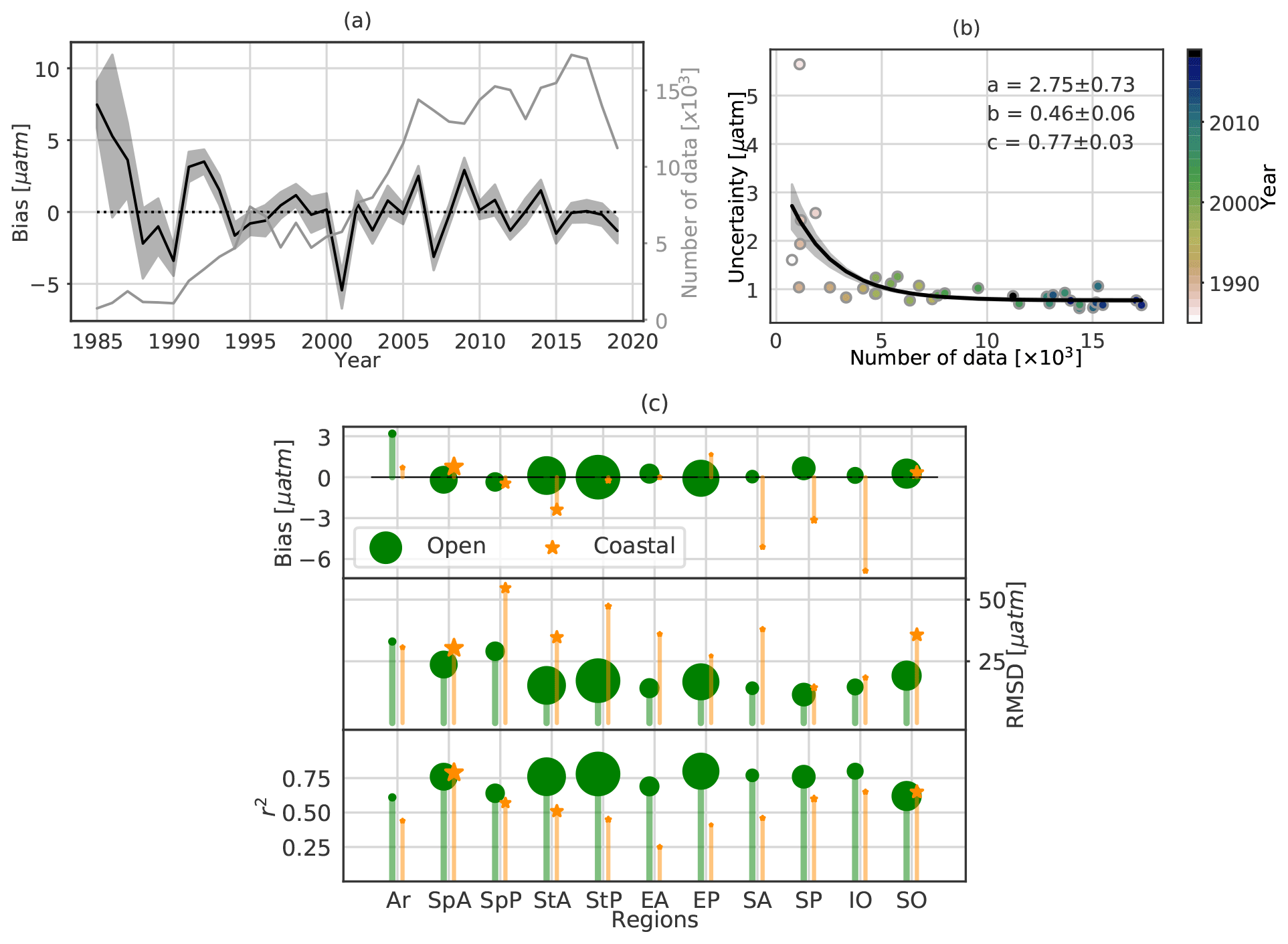
Figure 4(a) Time series of the yearly mean model bias, i.e. the reconstructed pCO2 data minus SOCATv2020 data, over the global ocean. The black curve and dark grey area represent the mean estimate and 1σ envelope of errors of the 100-member ensemble; the light grey curve represents the total number of gridded SOCAT data used in the FFNN model construction. (b) Exponential fits of the model uncertainty (the magnitude of the 1σ envelope in Fig. 4a) against the number of gridded data per year. The exponential function is . The black curve is derived from the best fit, and the grey-shaded area corresponds to the spread derived from standard errors of parameter estimates. (c) Statistical scores for 11 oceanic regions with the size of each scattered object proportional to the number of regional data (Table S2).
The model scores for the open ocean over the period 1985 to 2019 are 17.87 µatm for the RMSD and 0.78 for r2. The skill of this novel method, which uses only two-thirds of SOCAT data for fitting each of 100 FFNN models, ranks similarly to those from alternative statistical reconstruction approaches (Rödenbeck et al., 2013; Landschützer et al., 2014; Gregor et al., 2019) which have been used to complement model-based estimates of the ocean carbon sink (Friedlingstein et al., 2019, 2020).
The CMEMS-LSCE-FFNN reconstruction over the coastal regions for the full period is roughly 2 times less effective than over the open ocean in terms of the RMSD (35.86 µatm), while it shows a rather good fit with r2=0.70. The high RMSD reflects high local model errors along the continental shelves (Fig. S3). For the 1998–2015 period, the CMEMS-LSCE-FFNN approach scored an RMSD of 35.84 µatm while a recent coastal reconstruction by Landschützer et al. (2020) obtained an error of 26.8 µatm (see their Table 1). The latter presents a global ocean pCO2 climatology product by unifying data over the same period from two conceptually equivalent reconstruction models: one covering the open ocean at a 1∘ × 1∘ resolution (Landschützer et al., 2016) and one targeting the coastal ocean at a 0.25∘ × 0.25∘ resolution (Laruelle et al., 2017). These previous reconstructions cover the coastal region with a broader definition (400 km distance from the seashore) than the MARCATS mask used in this study, leading to the differences in characteristics and numbers of evaluation data of pCO2. In addition, the CMEMS-LSCE-FFNN model was designed with the leave-p-out cross-validation approach excluding many more independent data from monthly model fitting for model evaluation than the previous models. Overall model errors remain high despite the increase in the spatial resolution and in the number of observations. Coastal and shelf seas are characterized by complex physical and biological dynamics leading to high variability at small scales. For instance, pCO2 levels over the Californian shelf can exceed 850 µatm, with a spatial gradient of pCO2 as large as 470 µatm over a distance of less than 0.5 km (Chavez et al., 2018; Feely et al., 2008). Clearly, further model improvement is needed in order to capture such high spatial and temporal variability in surface ocean pCO2 present in observations (see also Bakker et al., 2016; Laruelle et al., 2017, and references therein).
In the following subsections, we present and discuss the reconstruction skills for different ocean regions, as well as for open-ocean and coastal domains (Fig. 4c). Complete results including the numbers of gridded data, RMSDs, and r2 for each region are summarized in Table S2.
3.1.2 Ocean basins
Arctic
Data coverage is particularly sparse over the Arctic Ocean (Ar) with 50 to 220 grid boxes with observations per year since 2007 and an interruption in 2010 (Fig. S4). While continental shelves account for 50 % of the region's area, only one-third of the observation-based data are from coastal regions. Moreover, observations are seasonally biased towards ice-free summer months (Bakker et al., 2016). Though reconstruction standard errors are similar for open basins and coastal regions (RMSDs of 33.01 and 30.65 µatm, respectively), the coefficient of determination is higher over the open ocean (r2=0.61) compared to coastal seas (r2=0.44), suggesting a higher model skill over open basins. The close-to-zero bias of the coastal reconstruction shown in Fig. 4c results from the compensation between highly positive and negative values over the continental shelves of Alaska, the Canadian archipelagos, and the Barents and Kara seas (see Fig. S3); the yearly bias fluctuates within µatm (Fig. S4). Of all open-ocean regions, the Arctic reconstruction has the highest bias (3.19 µatm). Cold Arctic waters are characterized by low levels of surface ocean pCO2 due to the temperature effect on CO2 solubility and the seasonal drawdown of dissolved inorganic carbon (DIC) during summer months by intense biological production (Feely et al., 2001; Takahashi et al., 2009; Arrigo et al., 2010). Assuming that the Arctic predictors remain within the range of global relationships, the overestimation of pCO2 by CMEMS-LSCE-FFNN, as seen in Fig. 4c, suggests a possible underestimation of biological productivity. While this remains conjectural, we acknowledge a large uncertainty in the contribution of biological activity (net primary production, NPP) to surface ocean pCO2, as it is “proxied” by chlorophyll a derived from remote sensing (Maritorena et al., 2010; Babin et al., 2015). Overall, these scores point to the Arctic as a relatively poorly reconstructed region.
Atlantic
The North Atlantic stands out as a region with high data coverage (Fig. S1a) and a rapidly increasing number of data since 2000 (Fig. S4). A sustained sampling effort adds between 2000 and 4000 data each year to the database over the Subtropical Atlantic (StA) and Subpolar Atlantic (SpA) regions (including between 10 %–40 % of coastal data). The data density over the North Atlantic stands in strong contrast to the often fewer than 1000 gridded data per year collected over the Equatorial Atlantic (EA) and South Atlantic (SA) and their strong year-to-year variability.
The comparison between the reconstructed open-ocean pCO2 and evaluation data over the four sub-regions of the open Atlantic (Fig. 4c and Table S2) reveals small mean model–data differences, which together with the two other scores, identify the Atlantic as the basin with the highest reconstruction skill. RMSDs corresponding to the StA, the EA, and the SA are below 15.50 µatm, and r2 values are in the range of [0.69,0.77]. While a larger RMSD is obtained over the SpA (23.68 µatm), the r2 of 0.76 falls close to the upper end of the range determined for the three other regions. As discussed in Schuster et al. (2013), large temporal and spatial gradients of pCO2 as well as its variability driven by a diversity of physical and biological processes (e.g. surface ocean temperature gradients, biological production, vertical mixing, and horizontal advection of water masses) keep the analysis of pCO2 over the SpA challenging.
Despite accounting for over 59 % of the total coastal data, skilful data reconstruction over the coastal Atlantic regions remains difficult. RMSDs are in general above 30 µatm, and, with the exception of the coastal SpA (r2=0.79), below 51 % of the observed variance is predicted by the model over the other regions (StA, 0.51; EA, 0.25; SA, 0.46). The large model–data mismatch along the Atlantic continental shelves (Fig. S3) reflects the poor reconstruction of pCO2 over regions under the influence of upwelling systems (e.g. Moroccan coast, Benguela), large river discharges (e.g. Amazon, Congo, Florida, Mississippi), and the bottlenecks of gulfs or bays (e.g. Bahamas, English Channel).
Pacific
With the exception of the Subpolar Pacific (SpP), the number of observations has increased regularly over the Pacific basin. In recent years, there are from 1000 to 3500 grid boxes with observations recorded over the Subtropical Pacific (StP), the Equatorial Pacific (EP), and the South Pacific (SP) (Fig. S4). Forty percent of total open-ocean data belong to the StP and the EP in the years 1985–2019. Corresponding RMSDs are 17.15 and 16.68 µatm, with r2 above 0.78. Despite a data coverage below one-third of that reported for the two previous regions, the model proved skilful in reconstructing pCO2 over the SP (Fig. 4c) with an RMSD of 11.50 µatm and r2 of 0.76.
The overall good performance of the FFNN over these three Pacific sub-regions contrasts with its lack of skill over the open SpP. The data density is poor and highly variable. From before 1994, fewer than 250 gridded data per year are available to constrain the reconstruction, followed by several years of intense effort and a maximum of about 1250 data in 2000 before decreasing again to the pre-1994 values. At first order, skill scores fluctuate in line with data density. During the first period (up to 1994), the bias varies within µatm (Fig. S4); it decreases close to µatm between 1997 and 2000 and increases again along with decreasing data density. Much like the SpA, the SpP is a region characterized by a strong spatial and temporal variability in pCO2 (Ishii et al., 2014), challenging any reconstruction method. The difficulty is further aggravated by the paucity of data in this region compared to the SpA. Skill scores are modest over the SpP with an RMSD of 29.08 µatm and r2 of 0.64 (Fig. 4c and Table S2).
The ratio between coastal and open-ocean observation-based data is 1 : 24. The paucity of data for the coastal domain is reflected by lower skill scores compared to the open ocean. Over the coastal SpP, for example, the RMSD amounts to 54.69 µatm, while it is 29.08 µatm for the corresponding open-ocean region. Comparable to the SpP, data reconstruction over the coastal regions of the StP (e.g. North American coast, Sea of Japan), as well as over the western EP (e.g. Peruvian upwelling) and the SP (e.g. offshore Chile), remains difficult (Fig. S3). Similar results have been found by Landschützer et al. (2020).
The EP is characterized by strong equatorial upwelling, making it one of the major outgassing regions of CO2 (Feely et al., 2001). Surface ocean pCO2 shows a strong interannual variability predominantly in response to the El Niño–Southern Oscillation (ENSO), the dominant regional climate mode (Rödenbeck et al., 2015; Landschützer et al., 2016; Denvil-Sommer et al., 2019). Before the 2000s, negative (positive) peaks of bias (Fig. S4) coincide with La Niña years, e.g. 1988–1990, 1995–1996, 1999–2001 (El Niño years, e.g. 1986–1987, 1991–1992, 1997–1998) (see the ENSO events highlighted in Fig. 9). A strong negative bias is again computed in 2010–2012, which could reflect the lack of data during that cooling phase. On the contrary, the reconstruction seems less sensitive to the strong warm anomalies associated with the 2015–2016 El Niño. The model appears to be more efficient at reconstructing surface ocean pCO2 during the hot climate mode (El Niño) than during the cool one (La Niña) when enhanced upwelling drives surface ocean pCO2 up and towards unusually large values. This allows us to anticipate the effect of a general decrease in data collection and processing since 2020 in response to the 2019 coronavirus disease (COVID-19) pandemic on the estimation of the ocean carbon sink. We expect a high negative bias in model estimates of pCO2 and the consequent underestimation of CO2 outgassing due to the combined impact of data decreasing and La Niña conditions governing since August and September 2020 (https://public.wmo.int/en/media/press-release/la-nina-has-developed, last access: December 2020). It is worthwhile to also note that monthly gridded SOCAT data in the eastern EP have declined in the last 5 years compared to the other years in the 2010s.
Indian Ocean
The Indian Ocean (IO) is the third-largest oceanic region by area but also the one with the lowest data density. With the exception of the year 1995 (approximately 1900 grid boxes including observations), as few as 500 gridded data have been provided per year (Fig. S4), yielding a total number of data often below 10 per grid cell for the entire reconstruction period (Fig. S1a). There have been even fewer than 75 grid boxes with observations per year over the continental shelf. However, the reconstruction over the coastal region is comparable to the open IO with a low RMSD (<19 µatm) and a high correlation with the observation-based data (r2=0.65). The overall negative bias shown in Fig. 4c for the coastal IO points to the model underestimating coastal pCO2 levels. Large errors are distributed along the western Arabian Sea, western Madagascar, and the tropical eastern IO (Fig. S3). These regions are under the influence of the southwest monsoon, giving rise to a seasonal upwelling regime (see Feely et al., 2001; Sabine et al., 2002; Sarma et al., 2013, and references therein). Strong seasonal upwelling results in a marked seasonal cycle of surface ocean pCO2 with high levels during the upwelling season. The paucity of data is likely to limit the skill of the model reconstruction of the seasonal cycle over large parts of the IO with consequences for the annual mean analysed here.
Southern Ocean
Until recently, data coverage over the Southern Ocean (SO) was sparse (Fig. S1a), irregular at the grid cell scale, and biased towards austral summer months (e.g. Bushinsky et al., 2019; Gregor et al., 2019). A strong sampling effort allowed a recent increase in observations to reach up to 2000 gridded data per year (Fig. S4). Model scores for the open and the coastal ocean are RMSDs of 19.18 µatm and 35.73 µatm, respectively, and r2 values of 0.62 and 0.65, respectively. The reconstruction lacks skill over the continental shelves of South America and Antarctica (see Fig. S3).
In general, the pCO2 reconstruction over the SO has less skill compared to the Atlantic or the Pacific due to the paucity of observation-based data compared to its large area. Rödenbeck et al. (2015) reported inconsistent reconstructed interannual variability in pCO2 between different data-based methods. The interannual variability is large due to the natural variability in the coupled ocean–atmosphere system characterized by one of the globe's strongest ocean currents, strong winds, and vertical mixing and upwelling of DIC-rich deep waters (Gregor et al., 2018; Gruber et al., 2019). Efforts to improve pCO2 reconstruction are ongoing and include model development (e.g. Gregor et al., 2017), as well as the increase in data coverage by the addition of data from different sampling platforms (e.g. profiling floats; Bushinsky et al., 2019). For the time being, CMEMS-LSCE-FFNN stands out as one of the skilful models with respect to observation-based data in the SO (Friedlingstein et al., 2020; Hauck et al., 2020).
3.1.3 Time series stations
CMEMS-FFNN-LSCE estimates of pCO2 are now compared with moored pCO2 time series provided by Sutton et al. (2019). This data product comprises pCO2 measurements collected from a wide range of oceanic regions since 2004 (Figs. S5–S8). Most of the stations were established in the North Atlantic and the North Pacific and Equatorial Pacific; one site is in the IO and another in the SO. Approximately one-third of the Sutton et al. (2019) sites belong to the coastal seas and shelves (Fig. S8). Table S3 details the information of the moored pCO2 time series.
Observation-based data used for model–data comparison (black points in Figs. S6–S8) are monthly averages of pCO2 measurements at each site. This interpolation results in monthly time series with a number of data N between 9 (NH10) and 98 (WHOTS). The ensemble mean μensemble and ensemble spread σensemble (Eq. 2) are computed from the CMEMS-LSCE-FFNN ensemble of model outputs at the four nearest model grid boxes of each location. Results confirm a reasonably good reconstruction of the proposed approach. The model best estimates (thick coloured lines) characterize pCO2 trends and variations in in situ data well, and the model ensembles almost catch the observation-based data in their 99 % confidence interval (light shaded envelope). For over 90 % of the time series stations, the model estimation obtains a moderate to high coefficient of determination r2 with a linear model–data correlation r larger than 0.5 (e.g. BTM, 0.98; CRESCENTREEF, 0.92; HOGREEF, 0.84; SOFS, 0.79; TAO110W, 0.75; WHOTS, 0.73). Mean bias μmisfit (Eq. 3) and the RMSD (Eq. 4) are relatively low compared to mean pCO2 values of the time series stations.
Half of the open-ocean reconstructions have model errors of less than 20 µatm and are even less than 10 µatm at KEO, PAPA, SOLS, STRATUS, and WHOTS (Figs. S6 and S7). Despite having less skill than the open-ocean reconstructions, the coastal-ocean reconstructions are quite compatible with the in situ data (Fig. S8). Most of the RMSDs remain lower than 20 % of the mean pCO2 values of coastal time series (e.g. CCE2, 36.53 µatm; ICELAND, 12.26 µatm; M2, 36.58 µatm). For some other stations on the US west coast and in the oceanic regimes of coral reef, the estimates differ from the observation-based data in terms of the magnitude of pCO2 (e.g. CRIMP2, LA PARGUERA) and/or of its seasonal cycle (e.g. CHABA, CHEECAROCKS, SEAK).
The reconstructed time series cover the full period 1985–2019, while observation-based data are still sparse and almost all distributed over the past 2 decades (Figs. S6–S8). The CMEMS-LSCE-FFNN time series would be useful for estimating and assessing long-term means, trends, and variations in CO2 surface partial pressure and the corresponding air–sea fluxes.
3.2 Long-term mean and uncertainty estimates
Figure 5 shows temporal mean estimates, their associated uncertainty, and RMSDs of the monthly air–sea pCO2 gradient (ΔpCO2) and CO2 fluxes (fgCO2) over the full period (see also Fig. S9 for the coastal regions only). On the top maps, the regions in blue are dominant CO2 uptake regions (influxes) and the regions in red are dominant source regions of CO2 to the atmosphere (effluxes). The uncertainty in ΔpCO2 is merely computed from the ensemble of the reconstructed sea surface pCO2 since the randomness in the atmospheric pCO2 field is assumed to be negligible. Due to impacts of wind stress, the solubility of CO2, and seasonal sea-ice coverage on the gas transfer coefficient, spatial distributions of mean estimates, their uncertainty, and RMSDs of ΔpCO2 (Fig. 5a, c, e) and fgCO2 (Fig. 5b, d, f) differ from low to high values. The means of air–sea fluxes integrated/averaged over different RECCAP1 regions (Table 1) are shown in Fig. 6. The distribution of uncertainty estimates and numbers of gridded SOCAT data for these regions are also displayed in Fig. 7, wherein only values smaller than the 90 % quantile of uncertainty estimates shown in Fig. 5c and d are plotted to reduce the effects of outliers on data visualization. The seasonal average computed over the full reconstruction period of air–sea CO2 fluxes over the global ocean is shown in Fig. 8.
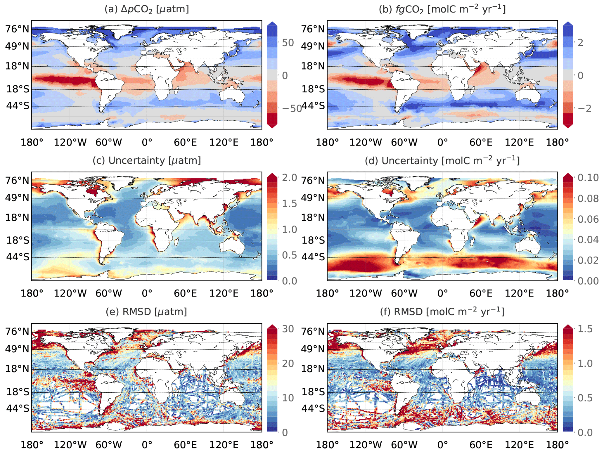
Figure 5Climatological mean (a, b) and uncertainty (c, d) of air–sea pCO2 difference (a, c) and of CO2 fluxes (b, d) over 1985–2019. Uncertainty (Eq. 2) is computed as the standard deviation of the 100-member CMEMS-LSCE-FFNN model outputs of sea surface pCO2 and air–sea CO2 fluxes. The bottom panels (e, f) show RMSDs (Eq. 4) between the SOCAT data (or data-based estimates of fluxes for f) and the mean CMEMS-LSCE-FFNN model outputs.
Table 2Yearly mean of contemporary air–sea CO2 fluxes (PgC yr−1) integrated over the global ocean and 11 RECCAP1 regions. The mean estimate and uncertainty (μensemble±σensemble) of the CMEMS-LSCE-FFNN approach is shown for the coast (C), the open ocean (O), and the total area (T). For a comparison, estimates derived from RECCAP1 (Canadell et al., 2011; Schuster et al., 2013; Ishii et al., 2014; Sarma et al., 2013; Lenton et al., 2013; Wanninkhof et al., 2013) are provided. In column “RECCAP1”, values in parentheses are the “best” estimates proposed by RECCAP1 studies which were derived from averages or medians of estimates based on the pCO2 climatology or pCO2 diagnostic model and/or the atmospheric and ocean inversions and GOBMs. The RECCAP1 values outside of parentheses are the estimates derived from different methods mapping observation-based data of pCO2. With an exception for the global estimate (denoted by *) (Wanninkhof et al., 2013), those of the RECCAP1 sub-basins are available only for the open ocean.
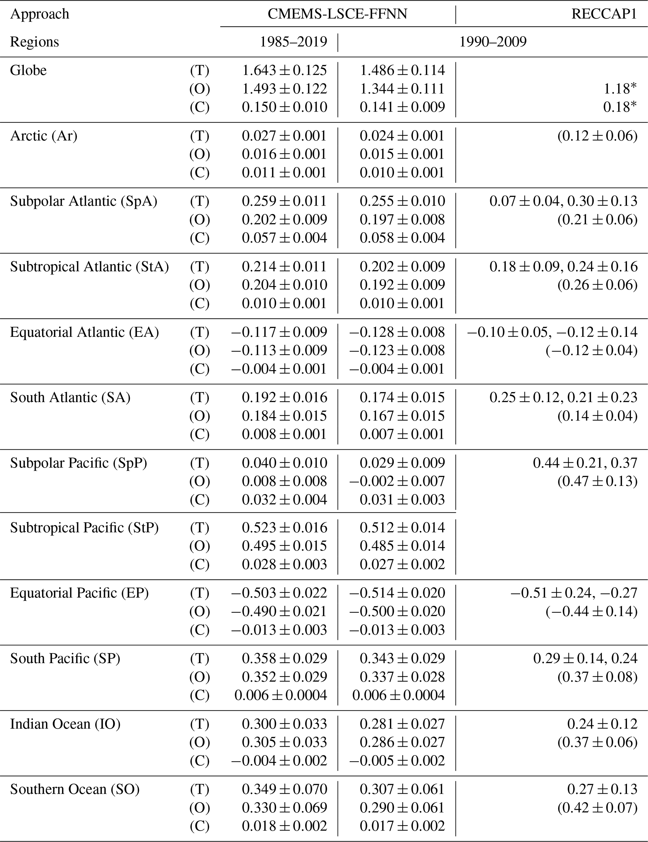

Figure 6Distribution of contemporary fluxes (positive into the ocean) over 11 regions (see in Fig. 2) for the full period 1985–2019. Uncertainties in the mean estimates of air–sea fluxes integrated (a) or averaged (b) over each region are shown with error bars.

Figure 7Distribution (violin) of all uncertainty estimates (Fig. 5c and d) and the total number (star) of gridded SOCAT data (Fig. S1a) split for 11 RECCAP1 regions. A violin plot shows the range, median, and density of uncertainty estimates for pCO2 (µatm) and fgCO2 (molC m−2 yr−1).
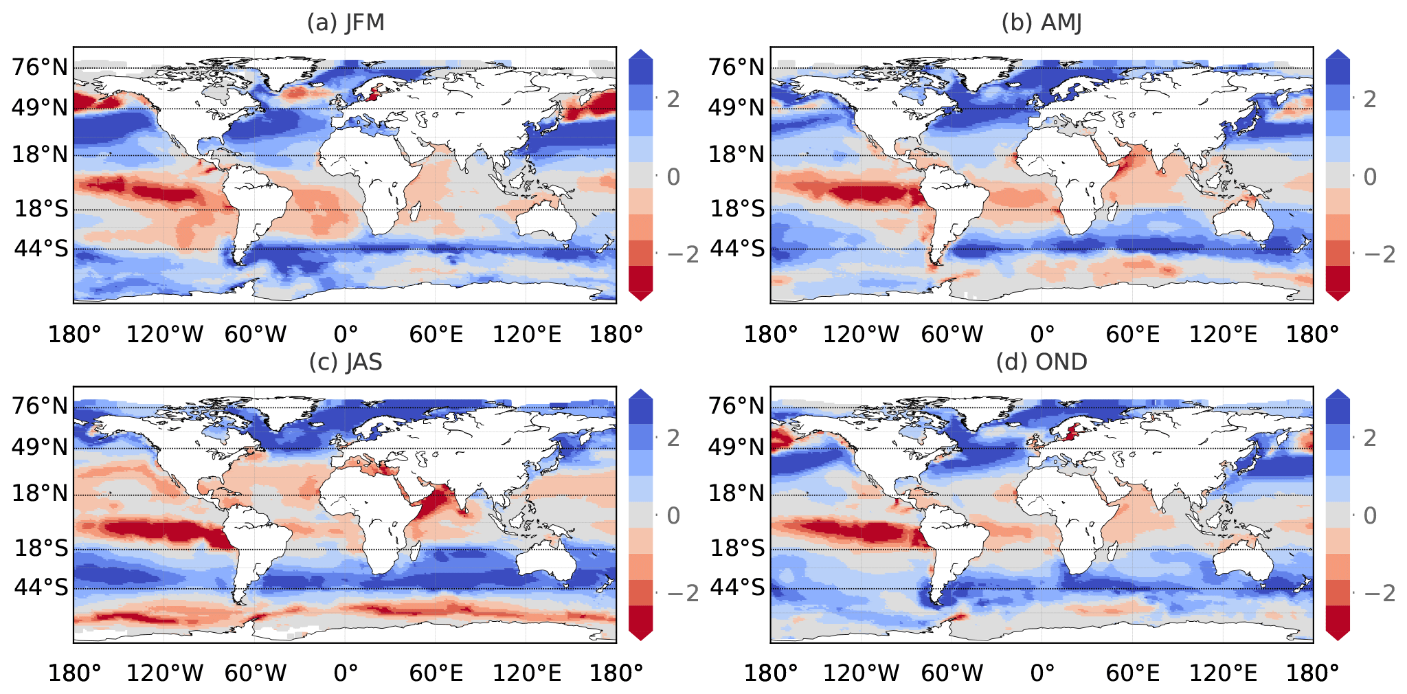
Figure 8Seasonality of downward CO2 fluxes (molC m−2 yr−1) in 1985–2019. Temporal means of the reconstructed fgCO2 field for January to March (JFM), April to June (AMJ), July to September (JAS), and October to December (OND) are shown.
3.2.1 Arctic
The Arctic Ocean stands out as the region with the strongest CO2 uptake per unit area with 2.336±0.104 molC m−2 yr−1 for the open sea and 1.522±0.108 molC m−2 yr−1 for the continental shelf margins (Figs. 5b and 6b). At the scale of grid cells, air–sea gradients of pCO2 are large, but the downward fluxes are relatively modest over the shelves of eastern Greenland, the Barents and Kara seas, and the Siberia seas (Figs. 5 or S9). During the sea-ice-covered seasons, these coastal regions are neutral while the open-ocean Arctic sectors (e.g. the Norwegian Sea, the Barents Sea, the Kara Sea) are CO2 sinks with moderate influx densities (Fig. 8). The open-ocean influx density exceeds 3 molC m−2 yr−1 in the Arctic summer. This substantial amount of CO2 uptake is driven by low surface ocean temperature, seasonal changes in sea-ice cover, and intense biological production. Increasing light availability and input of nutrients through meltwaters and river discharges sustain high levels of primary production and CO2 drawdown (Bates and Mathis, 2009; Arrigo et al., 2010; Yasunaka et al., 2016, 2018). Notwithstanding, the Arctic Ocean represents roughly 0.58 % of the total surface ocean area (Table 1), and the yearly mean CO2 uptake integrated over the Arctic for the full period amounts to only 1.64 % of the global ocean sink (Table 2 and Fig. 6a).
3.2.2 Atlantic
The open-ocean Subpolar Atlantic (SpA) sink contributes approximately 78 % to the total SpA annual C uptake (0.259±0.011 PgC yr−1), as well as 12.29 % to the total ocean sink (1.643±0.125 PgC yr−1, Table 2). Per unit area, the open-ocean influx amounts to 2.012±0.092 molC m−2 yr−1 and the coastal-ocean influx is 30.51 % less than its open-ocean counterpart and slightly lower than the coastal Arctic sink (Fig. 6b). However, when integrated over the region, the yearly uptake of 0.057±0.004 PgC yr−1 makes the coastal SpA the strongest sink among the 11 coastal regions (Fig. 6a). The interplay between temperature- and biology-driven effects results in changes in the seasonal and spatial distributions of surface ocean pCO2 and ultimately air–sea CO2 fluxes. During boreal winter–spring, high wind speeds enhance gas transfer velocities and contribute to a strong cooling and an increase in CO2 solubility (Takahashi et al., 2009; Feely et al., 2001), both enhancing uptake of CO2 over the Labrador Sea, the North Atlantic and Norwegian currents, and the Barents and Kara seas (Fig. 8). High wind speeds also strengthen vertical mixing, a process supplying dissolved inorganic carbon (DIC) and nutrients to the surface ocean. During the spring and summer months, vigorous biological activity (Sigman and Hain, 2012) counteracts the warming-induced decrease in CO2 solubility and increase in pCO2 by drawing down DIC (Feely et al., 2001). Along the coast of the Barents and Kara seas, inputs of fresh water (decrease in salinity and increase in CO2 solubility) and nutrients (biological activity and DIC drawdown) combine to strengthen CO2 uptake (Arrigo et al., 2010; Yasunaka et al., 2016, 2018; Olafsson et al., 2021). This contrasts with other coastal regions (e.g. southern North Sea and Baltic Sea) where the respiration of terrestrial particulate organic carbon from river run-off contributes to making these areas a strong seasonal source of CO2 (Borgesa and Gypensb, 2010; Becker et al., 2021).
The Subtropical Atlantic (StA) is characterized by weak to moderate mean flux densities per unit area (open, 0.733±0.036 molC m−2 yr−1; coastal, 0.457±0.064 molC m−2 yr−1). The total integrated C uptake amounts to 0.214±0.011 PgC yr−1, with 0.204±0.010 PgC yr−1 contributed by the open ocean. As for the SpA, the net uptake reflects the combined effect of cooling, mixing, and biological activity. Figures 5 and S9 show the regional distribution of sources and sinks. Regions of intense CO2 uptake are associated with the warm Gulf Stream and its northeastward extension, the North Atlantic Drift. Strong uptake is also found over the western continental shelf where strong river discharges sustain high levels of biological productivity, in particular during spring (Jamet et al., 2007; Kealoha et al., 2020). Weaker sinks or sources of CO2 in the southwestern StA and the eastern subtropical gyre are primarily driven by high surface temperature and enhanced stratification (Schuster et al., 2013). The latter restricts the vertical supply of nutrients and limits biological production. Finally, a relatively strong source of CO2 is found over the Canary upwelling system in summer (Fig. 8).
The Equatorial Atlantic (EA) stands out as the second-strongest source region of CO2 after the Equatorial Pacific (EP) with a yearly outgassing of PgC yr−1 (Fig. 6a). Most CO2 is released from the open ocean with an average efflux of (Figs. 5b and 6b). This intense source of CO2 stems from upwelling of cool and CO2-rich waters in the eastern EA. A westward increase in outgassing is observed along with the advection of CO2-rich waters (Schuster et al., 2013). The coastal EA regions release an average of molC m−2 yr−1 of CO2. Over large areas, the opposing effects of primary production and high surface temperature combine to weaken the coastal sink or seasonally switch it from a weak to a moderate source (e.g. the northeast EA, Caribbean Sea, Venezuelan and Guiana basins, Gulf of Guinea) (Fig. 8). The Amazon River is a notable exception. Its large discharges of fresh water and nutrients, as well as of dissolved and particulate carbon, turn the coastal and adjacent shelf seas into a net sink of CO2 (Medeiros et al., 2015; Ibánhez et al., 2015).
The South Atlantic (SA) uptake amounts to 0.192±0.016 PgC yr−1. Regions north of 30∘ S act as weak sources or are neutral with respect to air–sea exchanges of CO2, as opposed to regions to the south which are significant sinks of CO2 (Fig. 5b). For the full period, densities over the open and coastal regions are 0.862±0.072 and 0.776±0.125 molC m−2 yr−1, respectively. Coastal regions are changing from moderate sources to sinks with increasing latitude (Fig. S9). The SA has similar seasonal dynamics to the StA with CO2 uptake in winter and outgassing in summer (Takahashi et al., 2009; Schuster et al., 2013). During the austral winter, deep mixed layers result in cold surface waters which absorb CO2 from the atmosphere. By contrast, warming during the summer reduces the solubility of CO2, leading to a weak sink or even a source (Fig. 8). As explained before, biological production counteracts the effect of warming, and the vigorous spring bloom contributes to the uptake south of 30∘ S (Sigman and Hain, 2012; Carvalho et al., 2020).
3.2.3 Pacific
The Subpolar Pacific (SpP) is the second-smallest region by area (2.78 % of the total surface ocean area) and with 0.040±0.010 PgC yr−1 (net coastal and open-ocean sinks) provides the smallest contribution to the total yearly ocean C uptake (Table 2 and Fig. 6a). The coastal ocean contributes about 0.032±0.004 PgC yr−1 to the total yearly C uptake, making the SpP the only region for which coastal fluxes exceed open-ocean fluxes. The strength of its coastal C sink ranks second among all coastal regions (Fig. 6a). Seasonal features of CO2 fluxes are shown in Fig. 8. The SpP is ice-covered during the winter months, which results in close-to-zero air–sea fluxes per unit area north of 60∘ N (e.g. Beaufort, Siberia, and Chukchi seas). Besides, vertical convection during winter brings up old DIC-rich waters, leading to CO2 outgassing exceeding −3 molC m−2 yr−1 in the south of the region (Bates and Mathis, 2009; Arrigo et al., 2010; Ishii et al., 2014; Yasunaka et al., 2016). Intense biological production during the boreal summer drives intense uptake of CO2 over the entire SpP (Feely et al., 2001; Sigman and Hain, 2012; Ishii et al., 2014). The interplay of these two seasonal mechanisms and their opposing effects make the open SpP a weak yearly net sink (Fig. 6). The average flux density per unit area is 0.044±0.123 molC m−2 yr−1 over the open ocean, much smaller than the value determined for the coastal ocean of 0.775±0.127 molC m−2 yr−1 (Fig. 6b). As shown in Bates (2006), Arrigo et al. (2010), and Ishii et al. (2014), surface DIC concentration is higher over the open, deep basins than the shallow coastal seas of the SpP, particularly induced by deep mixing during winter and spring. Over the same period, seasonal sea ice also restricts gas exchange; the coastal sector thus acts as a neutral region of CO2 fluxes (Fig. 8). During spring and summer, a substantial amount of CO2 is also absorbed in the coastal shelf seas influenced by high biological production in large ice-free areas (e.g. Chukchi and Gulf of Alaska) and/or by dilution of seawaters from river fresh water with low salinity and DIC concentration (e.g. Beaufort, Laptev, and East Siberian seas) (Arrigo et al., 2010; Yasunaka et al., 2016, 2018).
A total mean uptake of 0.523±0.016 PgC yr−1 makes the Subtropical Pacific (StP) the largest sink region. The open-ocean contribution dominates the regional sink with 0.495±0.015 PgC yr−1 (Table 2 and Fig. 6a). The corresponding mean flux density per unit area is 1.136±0.036 molC m−2 yr−1 (Fig. 6b) and makes the StP rank third after the open-ocean Arctic and SpA regions. As discussed for the StA, during winter months cooling and high wind intensities along the Kuroshio and North Pacific currents enhance the uptake of CO2 (Takahashi et al., 2009; Ishii et al., 2014). By contrast, summer warming drives the StP towards close-to-neutral conditions or a weak source (Fig. 8). With a yearly mean uptake of 0.028±0.003 PgC yr−1, the coastal StP sink ranks third in terms of intensity among the coastal sinks (Fig. 6a). The influx density is 1.444±0.130 molC m−2 yr−1. Western coastal systems and shelf seas are under the influence of the delivery of fresh water and nutrients by large river systems (Liu et al., 2014). The resulting intense biological production contributes to influx densities per unit area that are higher over the western continental shelf and seas (e.g. East China Sea, Sea of Japan) than over the California upwelling system (Figs. 5b, S9b, and 8).
The Equatorial Pacific (EP) is the strongest source region of CO2 to the atmosphere with a yearly average efflux of PgC yr−1 from the open ocean and PgC yr−1 from the continental shelves. On average per unit area, the open sea emits molC m−2 yr−1 of CO2. This high rate of outgassing is a distinct feature of the EP (e.g. Feely et al., 2001; Takahashi et al., 2009; Rödenbeck et al., 2015; Landschützer et al., 2016; Denvil-Sommer et al., 2019; Landschützer et al., 2019) and is primarily due to the upwelling of DIC-rich deep waters. The magnitude of CO2 release decreases westwards – from eastern boundary upwelling (e.g. Peru, Panama) to the International Date Line – in line with decreasing upwelling intensity, warmer sea surface temperature, and lower salinity (Ishii et al., 2014). Compared to the open EP, the efflux density of the coastal regions ( molC m−2 yr−1) is roughly half that of the open ocean.
The South Pacific (SP) ranks second as a sink region for CO2 with a yearly net flux of 0.358±0.029 PgC yr−1, mostly contributed by the open ocean (Fig. 6a). Uptake rates per unit area are very similar to those obtained for the SA (Fig. 6b). A detailed assessment reveals the open-ocean influx density to be slightly lower (0.791±0.066 molC m−2 yr−1) and the coastal one to be slightly higher (0.987±0.063 molC m−2 yr−1) over the SP compared to the SA. Due to the larger area of the SP (Table 1), its integrated sink is approximately twice that of the SA. Similarly to the processes discussed above for the SA, vertical mixing drives the uptake of CO2 during austral winter (Takahashi et al., 2009; Ishii et al., 2014), and the effect of warming on CO2 solubility during spring and summer is offset by biological production. The biological production leads to moderate to high uptake of CO2 over the coasts and the southwest open sea (e.g. East Australian Current, southern Australia, New Zealand) (Fig. 8). The influx density decreases eastwards under the influence of the strong upwelling of DIC driven by the Peru Current.
3.2.4 Indian Ocean
The total integrated Indian Ocean (IO) sink is evaluated to 0.300±0.033 PgC yr−1, with 0.305±0.033 PgC yr−1 contributed by the open ocean and a weak coastal source of PgC yr−1. The spatial distribution of flux densities (Fig. 5b) reveals the northwestern IO to be a net source of CO2 to the atmosphere, while the northeastern IO is close to neutral and latitudes south of 18 ∘S act as a strong sink. This regional compensation leads to a small open-ocean influx density per unit area of 0.482±0.052 molC m−2 yr−1 and a small coastal efflux per unit area of molC m−2 yr−1 (Fig. 6b). The northern IO is a strong source of CO2 sustained by the monsoon-driven seasonal upwelling along the Arabian and Somali coasts (Behrenfeld et al., 2006; Sarma et al., 2013). The northeastern IO regions including the Bay of Bengal and its continental shelves receive fresh waters discharged from the river Ganges and lateral inputs from Indonesian outflows (see Sarma et al., 2013, and references therein) and switch between mild sources and sinks (Fig. 8). A subtropical front (40∘ S) divides the region south of 18∘ S into a weak sink to the north and over an oligotrophic gyre and a band of vigorous uptake to its south over the Subantarctic Zone (SAZ) between 40 and 44∘ S (Fig. 5b). Similarly to the SA and SP, this entire region is identified as a significant net sink of CO2 in winter (Fig. 8), possibly driven by enhanced solubility in response to cooling and mixing. While biological production maintains the sink over the SAZ during austral spring and summer months, warming reduces CO2 uptake over the oligotrophic gyre.
3.2.5 Southern Ocean
The total Southern Ocean (SO) sink amounts to 0.349±0.070 PgC yr−1, including coastal uptake of 0.018±0.002 PgC yr−1. The mean influx per unit area over the open SO is 0.468±0.104 molC m−2 yr−1 and close to the one obtained for the open IO (Fig. 6b). The area-averaged CO2 drawdown over the coastal SO is 0.599±0.089 molC m−2 yr−1 with strong coastal sinks distributed over the South American and Antarctic shelves (60∘ westwards as seen in Figs. 5b or S4b). During the austral spring and summer, intense phytoplankton blooms enhance the consumption of CO2 over the Subantarctic Zone and the Polar Frontal Zone between 44 and 58∘ S (Sigman and Hain, 2012; Lenton et al., 2013), leading to a large sink with a flux density exceeding 1.667 molC m−2 yr−1 (Fig. 8). South of 58∘S, sea-ice retreat and vertical stratification contribute to a mild sink over the Antarctic Zone. During winter, vertical mixing brings DIC-rich deep waters to the surface, triggering strong outgassing of CO2 along the Antarctic Circumpolar Current.
4.1 Contemporary air–sea CO2 flux estimates
Our estimates of contemporary net fluxes of CO2 for the global ocean and 11 open-ocean regions are compared to estimates from RECCAP1 in Table 2 after adjusting them to the same period (1990–2009). RECCAP1 best estimates were derived from averages or medians of estimates based on the pCO2 climatology or pCO2 diagnostic model and/or the atmospheric and ocean inversions and GOBMs (see Schuster et al., 2013; Ishii et al., 2014; Sarma et al., 2013; Lenton et al., 2013, and references therein). The observation-based estimates of regional net fluxes reported in these studies were computed from the reconstruction of SOCAT pCO2 data (only used in Schuster et al., 2013), Lamont-Doherty Earth Observatory (LDEO) data (https://www.ldeo.columbia.edu/res/pi/CO2/, last access: 16 February 2022), and their climatology (Takahashi et al., 2009). With the exception of the global ocean, coastal fluxes were not part of the earlier assessment. The global open-ocean uptake obtained in this study of 1.344±0.111 PgC yr−1 lies between the observation-based net sink estimate by Wanninkhof et al. (2013) (1.18 PgC yr−1) and the global sum of regional best estimates given in Table 2 (1.8 PgC yr−1). Net regional fluxes computed from CMEMS-LSCE-FFNN are mostly within the range of fluxes derived from observation-based reconstructions and multi-approach best estimates. Our Southern Ocean open-ocean sink (0.290±0.061 PgC yr−1) compares well with previous observation-based estimates (0.27±0.13 PgC yr−1) but is lower than multi-approach best estimates (0.42±0.07 PgC yr−1). A significant discrepancy between the present and previous estimates is also found over the Arctic Ocean, for which the regional open-ocean net CO2 uptake is about 1 order of magnitude lower in CMEMS-LSCE-FFNN compared to the RECCAP1 best estimate (Schuster et al., 2013).
Based on the MARCATS mask (Fig. 2), the CMEMS-LSCE-FFNN estimate of the yearly net coastal sink over the full reconstruction period is 0.150±0.010 PgC yr−1. For 1990–2011, we estimate a yearly net coastal sink of 0.147±0.009 PgC yr−1, which is lower than the one based on SOCATv2 data by Laruelle et al. (2014) (0.19±0.05 PgC yr−1). Despite the fact that the present estimate was obtained with a model at a lower spatial resolution, the flux density of coastal sources and sinks, as well as their spatial distribution (Fig. S9b), is, in general, consistent with Laruelle et al. (2014) (Fig. 2), with exceptions found in northern polar and subpolar regions. For instance, Laruelle et al. (2014) suggested the Okhotsk shelf was a strong source of CO2 in excess of −3 molC m−2 yr−1. To the contrary and in line with Otsuki et al. (2003), it is identified as a significant sink in this study taking up 1 to 2.333 molC m−2 yr−1 (Fig. 5).
Our estimates for the mean annual open-ocean and coastal-ocean uptake over the Arctic (>76∘ N) are 0.015±0.001 and 0.010±0.001 PgC yr−1 (Table 2), which are less than the best estimate of 0.12±0.06 PgC yr−1 by Schuster et al. (2013) and that of 0.07 PgC yr−1 by Laruelle et al. (2014), respectively. The discrepancy is possibly due to an overestimation of Arctic pCO2 by the CMEMS-LSCE-FFNN (see “Arctic” in Sect. 3.1.2) and to the lack of estimates over a large portion of the seasonally-sea-ice-covered regions (see Figs. 5 and 8). Further improvements would include using additional products of sea surface height and input from river discharge and sea-ice melt available over the Arctic. Besides, in Eq. (1), the air–sea flux density is a linear function of the sea-ice fraction leading to fgCO2=0 as fice=1. Loose et al. (2009) suggest that the flux density in such regions is larger than evaluated by Eq. (1). A suggestion for a better assessment of air–sea fluxes over the Arctic and other regions with sea-ice cover (i.e. Antarctic and partly subpolar regions) would be to impose a sea-ice concentration of 99 % for values exceeding 99 % (Bates et al., 2006).
4.2 Model errors and uncertainties
Our uncertainty evaluation for estimates of pCO2 and air–sea CO2 fluxes is based on a Monte Carlo approach. Statistics (i.e. ensemble standard deviation, Eq. 2) are based on ensembles of CMEMS-LSCE-FFNN model realizations. This allows producing spatially and temporally varying uncertainty fields of pCO2 and fgCO2 estimates covering the global ocean and the full period. This asset can be used for quantifying the uncertainty for different spatial and temporal resolutions (e.g. monthly/yearly integrated fluxes at regional/global scales).
As a complement to Fig. 3 (bottom plots), which generally evaluates the reliability of model uncertainty estimates compared to model–data misfit deviations, Fig. 5 shows some similarity between their spatial distributions for pCO2 (Fig. 5c and e) and for fgCO2 (Fig. 5d and f). For pCO2, large model–data misfits and uncertainties are found over regions not only with sparse density or devoid of SOCAT data (see Figs. S1a and S4) but also with high temporal and/or spatial pCO2 variations (partly shown in Fig. S1b and c). High temporal/spatial gradients of pCO2 are typically associated with upwelling systems (e.g. eastern boundary upwelling systems, Arabian Sea upwelling), western boundary currents (e.g. Gulf Stream, Kuroshio), intense biological production (e.g. spring bloom in temperate northern/southern latitudes), coastal and shelf dynamics including river run-off (e.g. the Amazon, Congo, and Mississippi and great subpolar and Arctic rivers such as the Ob, Yenisey, Lena, Mackenzie). Comparing between Fig. 5c and Fig. 5d (Fig. 5e and Fig. 5f), the magnitude of the uncertainty estimates (model errors) of air–sea CO2 flux estimates appears to be much less correlated to measurement density (Fig. S1) than the pCO2 field (see also Fig. 7a and b). The model uncertainty and errors in fgCO2 estimates are highest over the open SO (>44∘ S), the subpolar regions, the Indian Ocean gyre, and upwelling systems.
In this study, the uncertainty quantified for the reconstruction of pCO2 and ultimately fgCO2 is a result of randomly sampling training and validation datasets from predictors and SOCAT observation-based data for 100 FFNN model runs (see Sect. 2.2). This sub-sampling approach permits taking into account an assumption about uncertainties in predictors and SOCAT data; i.e. random errors exist through changes in the range between their sub-samples. For a better assessment of the reconstruction uncertainty, future studies would need to include realistic uncertainties in these data, and also in local (sub-)skin effects of temperature and salinity as suggested in Watson et al. (2020). Additional sources of uncertainty in the computation of air–sea fluxes are discussed by Wanninkhof (2014), Woolf et al. (2019), and Fay et al. (2021). These studies have demonstrated the strong impact of different wind field products and model parameterizations on the gas transfer velocity k in Eq. (1) and the corresponding air–sea flux estimates. For instance, using the eight expressions for the parameterization of k proposed in Woolf et al. (2019) and references therein would inflate the uncertainty in the global mean annual uptake from 5 % to 10 %. However, it would not significantly impact the spatial distribution of uncertainty, only its magnitude.
4.3 Quantification of the global ocean carbon sink
Table 3 presents the comparison of estimates between the CMEMS-LSCE-FFNN, an ensemble of data-based reconstruction approaches, and an ensemble of global ocean biogeochemical models (GOBMs) used in the Global Carbon Project (GCP; Friedlingstein et al., 2019, 2020; Hauck et al., 2020) for the reconstruction of air–sea CO2 fluxes. The reconstructed CMEMS-LSCE-FFNN field covers approximately 88.9 % of the total ocean area used by the GCP (361.9×10⁶ km2). The annual contemporary uptake over the global ocean and the full period 1985–2019 was 1.643±0.125 PgC yr−1 with a starting net influx of 0.784±0.178 PgC yr−1, a growth rate of PgC yr−2, and an interannual variability (temporal standard deviation) of 0.526±0.022 PgC yr−1 (Fig. 9). The contemporary sink amounted to 2.301±0.126 PgC yr−1 for the last decade (2010s) and 2.877±0.154 PgC yr−1 in the year 2019 (Table 3). The long-term positive trend of the global ocean carbon sink estimates tracks the growth rate of atmospheric CO2 concentration since the mid-1980s (Friedlingstein et al., 2019, 2020). The interannual to multi-annual variability in the global ocean carbon sink co-varies with cold and hot ENSO phases (Fig. 9), confirming ENSO as a leading mode of variability in the ocean carbon sink (Feely et al., 1999).

Figure 9Yearly global integrated air–sea flux estimates derived from the CMEMS-LSCE-FFNN ensemble (mean ± uncertainty) for 1985–2019. The multivariate El Niño–Southern Oscillation index (MEI; Wolter and Timlin, 1993, https://psl.noaa.gov/enso/mei/, last access: December 2020) is used to generally indicate a link between variations, e.g. yearly uptake–trend, in the CMEMS-LSCE-FFNN sink estimate and the ENSO climate mode (El Niño, MEI > 0.5; La Niña, MEI < −0.5; neutral: otherwise).
Table 3Comparison of the global anthropogenic CO2 uptake (mean ± uncertainty) between CMEMS-LSCE-FFNN and data-based and model-based estimates used in the Global Carbon Project (Friedlingstein et al., 2019, 2020; Hauck et al., 2020). The CMEMS-LSCE-FFNN approach provides contemporary flux estimates. Anthropogenic flux estimates are derived from contemporary fluxes adjusted with the global ocean area of 361.9×10⁶ km2 and the riverine flux of 0.78 PgC yr−1. The estimates in parentheses were provided in Hauck et al. (2020) as the ensemble mean and standard deviation (μensemble±σensemble) of the model- or data-based estimates.
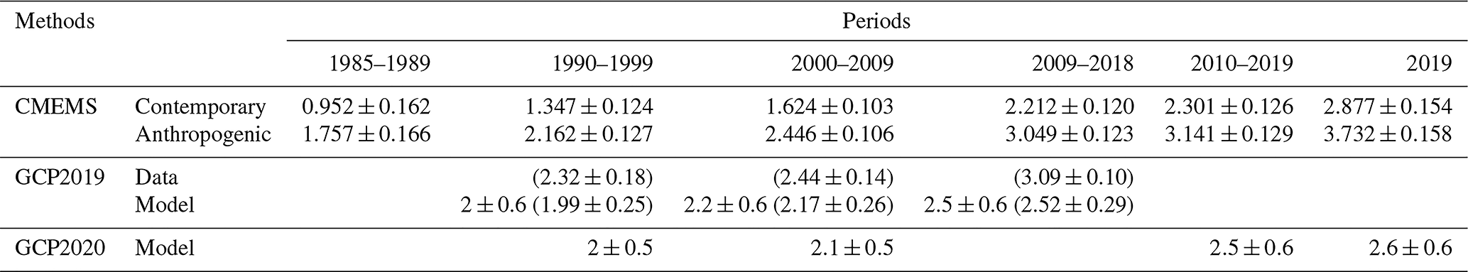
Taking into account the total ocean area of 361.9×10⁶ km2 and the outgassing of river carbon of 0.78 PgC yr−1 (Resplandy et al., 2018) yields an anthropogenic sink estimate of 2.423±0.125 PgC yr−1 for the years 1985–2019, 3.141±0.129 PgC yr−1 for the 2010s, and 3.732±0.158 PgC yr−1 for 2019. As shown in Table 3, the CMEMS-LSCE-FFNN estimates of the annual anthropogenic C uptake for different decades (1990s to 2010s) are in line with the data-based estimates but above the model-based estimates in the GCP publications. Hauck et al. (2020) demonstrated that the spatial distribution of CO2 sources and sinks, as well as decadal trends of the annual mean flux estimates derived from the data-based reconstruction methods and the GOBMs, is consistent at the global and regional scales. However, the mismatches in the magnitude of these estimates, seasonal cycles, and their interannual variability are still large and remain to be resolved. Note that the uncertainties computed in Hauck et al. (2020) (see estimates in parentheses in Table 3) are defined as the ensemble standard deviation of multiple data-based or model-based products and are lower than the uncertainties reported in the GCP (Friedlingstein et al., 2019, 2020). The latter published a total estimate of ±0.6 PgC yr−1, which corresponds to the combination of the interannual variability derived from GOBM-based estimates (±0.4 PgC yr−1) and the uncertainty in the ensemble mean ocean sink (±(0.2–0.4) PgC yr−1).
In this paper, we proposed an ensemble of 100 feed-forward neural network models for the reconstruction of air–sea fluxes of CO2 (fgCO2) over the global ocean for the period 1985–2019. This CMEMS-LSCE-FFNN model was first used to reproduce the pCO2 fields, and we have evaluated its skill. The corresponding monthly fields of fgCO2 were then deduced by applying the air–sea CO2 flux formulation (Eq. 1). Mean state estimates and uncertainty (Eq. 2) from the CMEMS-LSCE-FFNN ensemble-based estimates of air–sea CO2 fluxes have been analysed for the global ocean and 11 RECCAP1 sub-basins (Fig. 2) from the open seas to the continental shelves.
Our estimate for the contemporary net global sink over the period 1985–2019 is 1.643±0.125 PgC yr−1 including 0.150±0.010 PgC yr−1 for the coastal sink. The model suggested a net flux of 0.784±0.178 PgC yr−1 in the year 1985 followed by an increase in the global ocean uptake with a growth rate of PgC yr−2. CO2 absorption by the ocean showed little fluctuation in the 1990s followed by an anomalous reduction in the years 1999–2001 (Fig. 9). Thereafter, the ocean sink strengthened, leading to a global uptake rate of 2.301±0.126 PgC yr−1 in the 2010s. The large interannual to multi-year variations in the global carbon sink with a temporal standard deviation of 0.526±0.022 PgC yr−1 are associated with the ENSO climate variability.
The global ocean sink and regional sources and sinks of CO2 computed by CMEMS-LSCE-FFNN (Tables 2 and 3) were compared to the estimates by RECCAP1 (Canadell et al., 2011; Wanninkhof et al., 2013; Schuster et al., 2013; Ishii et al., 2014; Sarma et al., 2013; Lenton et al., 2013) and GCP (Friedlingstein et al., 2019; Hauck et al., 2020; Friedlingstein et al., 2020). We showed that the magnitude, spatial distribution, and seasonal variations in CMEMS-LSCE-FFNN CO2 fluxes are generally consistent with those suggested in the preceding studies (Feely et al., 2001; Takahashi et al., 2009; Laruelle et al., 2014, 2017) for both the open and the coastal seas. Mechanisms shaping the regional distribution (Figs. 5b and 6) and seasonal variations (Fig. 8) of net sinks and sources of CO2 were briefly discussed in Sect. 3.2. The results in Fig. 6 also suggest a difference between the rank of 11 RECCAP1 sub-basins with respect to their total net sinks or sources and with respect to their mean flux densities per unit area:
-
Ranking regional contributions to the global integration of air–sea fluxes. The EP is confirmed as the predominant ocean source region compensating for approximately 25 % of the total sinks for both the open and the coastal seas. The EA regions and the coastal IO are diagnosed as weak sources. Due to its large area, the open StP contributes the largest regional sink of CO2 to the global ocean net flux (the StP sink is equivalent to the EP source), followed by the SO, the IO, and the SP. For the coastal regions, the largest sink is computed for the SpA (one-third of the total coastal uptake), followed by the North Pacific and the SO.
-
Ranking mean regional flux densities per unit area. The EP remains the strongest source of CO2 followed by the EA and the coastal IO. The CO2 absorption is higher over the Northern Hemisphere than over the Southern Hemisphere, with the strongest uptake per unit area over the open Arctic and SpA. The coastal Arctic, SpA, and StP are identified as the dominant coastal sinks with similar flux densities.
Though statistics and relevant analyses throughout the paper have confirmed that the CMEMS-LSCE-FFNN estimates of sea surface pCO2 and air–sea CO2 fluxes are reasonably reliable, we believe that the model skill can be further improved. The spatial patterns of model–data misfit (RMSD between SOCAT data and the reconstructed fields, Eq. 4) and model uncertainty (ensemble standard deviation, Eq. 2) computed by the proposed approach (Fig. 5) agree in pointing out where the model poorly recovers evaluation data and/or results in large uncertainty estimates. We showed that the uncertainty fields (e.g. Fig. 5c and d) produced by the CMEMS-LSCE-FFNN approach are more informative than the standard error maps (e.g. Fig. 5e and f). Thus, the CMEMS-LSCE-FFNN uncertainty fields could be used to identify regions that should be prioritized in future extensions of the observational network and confirmed through dedicated observing system simulation experiments (Denvil-Sommer et al., 2021).
The dataset of sea surface pCO2 and air–sea CO2 fluxes analysed in this study is under the quality control of the European Copernicus Marine Environment Monitoring Service (CMEMS) and has been available for use since 2019. Our dataset can be downloaded through the CMEMS portal (https://doi.org/10.48670/moi-00047, Chau et al., 2020).
The supplement related to this article is available online at: https://doi.org/10.5194/bg-19-1087-2022-supplement.
TTTC, MG, and FC developed the CMEMS-LSCE-FFNN model. TTTC conducted numerical experiments and analysed results with support from MG and FC. All the authors contributed in preparing and completing the manuscript.
The contact author has declared that neither they nor their co-authors have any competing interests.
Publisher’s note: Copernicus Publications remains neutral with regard to jurisdictional claims in published maps and institutional affiliations.
The authors would like to thank the associate editor Jean-Pierre Gattuso, all the three referees, and Nicolas Metzl for their constructive comments, suggestions, and support to improve our manuscript. Many thanks go to everyone involved in data collection and processing of surface ocean CO2 fugacity. The Surface Ocean CO2 Atlas (SOCAT, https://www.socat.info, last access: 16 June 2020) is an international effort, endorsed by the International Ocean Carbon Coordination Project (IOCCP), the Surface Ocean Lower Atmosphere Study (SOLAS), and the Integrated Marine Biogeochemistry and Ecosystem Research (IMBER) programme, to deliver a uniformly quality controlled surface ocean CO2 database.
This research has been supported by the European Copernicus Marine Environment Monitoring Service (CMEMS) for the MOB TAC project in 2018–2021 (83-CMEMS-TAC-MOB contract, https://marine.copernicus.eu/about/producers/mob-tac, last access: 27 July 2021).
This paper was edited by Jean-Pierre Gattuso and reviewed by Meike Becker and two anonymous referees.
Arrigo, K. R., Pabi, S., van Dijken, G. L., and Maslowski, W.: air–sea flux of CO2 in the Arctic Ocean, 1998–2003, J. Geophys. Res.-Biogeo., 115, G04024, https://doi.org/10.1029/2009JG001224, 2010. a, b, c, d, e, f
Babin, M., Bélanger, S., Ellingsen, I., Forest, A., Le Fouest, V., Lacour, T., Ardyna, M., and Slagstad, D.: Estimation of primary production in the Arctic Ocean using ocean colour remote sensing and coupled physical–biological models: strengths, limitations and how they compare, Prog. Oceanogr., 139, 197–220, https://doi.org/10.1016/j.pocean.2015.08.008, 2015. a
Bakker, D. C. E., Pfeil, B., Landa, C. S., Metzl, N., O'Brien, K. M., Olsen, A., Smith, K., Cosca, C., Harasawa, S., Jones, S. D., Nakaoka, S., Nojiri, Y., Schuster, U., Steinhoff, T., Sweeney, C., Takahashi, T., Tilbrook, B., Wada, C., Wanninkhof, R., Alin, S. R., Balestrini, C. F., Barbero, L., Bates, N. R., Bianchi, A. A., Bonou, F., Boutin, J., Bozec, Y., Burger, E. F., Cai, W.-J., Castle, R. D., Chen, L., Chierici, M., Currie, K., Evans, W., Featherstone, C., Feely, R. A., Fransson, A., Goyet, C., Greenwood, N., Gregor, L., Hankin, S., Hardman-Mountford, N. J., Harlay, J., Hauck, J., Hoppema, M., Humphreys, M. P., Hunt, C. W., Huss, B., Ibánhez, J. S. P., Johannessen, T., Keeling, R., Kitidis, V., Körtzinger, A., Kozyr, A., Krasakopoulou, E., Kuwata, A., Landschützer, P., Lauvset, S. K., Lefèvre, N., Lo Monaco, C., Manke, A., Mathis, J. T., Merlivat, L., Millero, F. J., Monteiro, P. M. S., Munro, D. R., Murata, A., Newberger, T., Omar, A. M., Ono, T., Paterson, K., Pearce, D., Pierrot, D., Robbins, L. L., Saito, S., Salisbury, J., Schlitzer, R., Schneider, B., Schweitzer, R., Sieger, R., Skjelvan, I., Sullivan, K. F., Sutherland, S. C., Sutton, A. J., Tadokoro, K., Telszewski, M., Tuma, M., van Heuven, S. M. A. C., Vandemark, D., Ward, B., Watson, A. J., and Xu, S.: A multi-decade record of high-quality fCO2 data in version 3 of the Surface Ocean CO2 Atlas (SOCAT), Earth Syst. Sci. Data, 8, 383–413, https://doi.org/10.5194/essd-8-383-2016, 2016. a, b, c
Bates, N. R.: air–sea CO2 fluxes and the continental shelf pump of carbon in the Chukchi Sea adjacent to the Arctic Ocean, J. Geophys. Res.-Oceans, 111, C10013, https://doi.org/10.1029/2005JC003083, 2006. a
Bates, N. R. and Mathis, J. T.: The Arctic Ocean marine carbon cycle: evaluation of air-sea CO2 exchanges, ocean acidification impacts and potential feedbacks, Biogeosciences, 6, 2433–2459, https://doi.org/10.5194/bg-6-2433-2009, 2009. a, b
Bates, N. R., Moran, S. B., Hansell, D. A., and Mathis, J. T.: An increasing CO2 sink in the Arctic Ocean due to sea–ice loss, Geophys. Res. Lett., 33, L23609, https://doi.org/10.1029/2006GL027028, 2006. a
Becker, M., Olsen, A., Landschützer, P., Omar, A., Rehder, G., Rödenbeck, C., and Skjelvan, I.: The northern European shelf as an increasing net sink for CO2, Biogeosciences, 18, 1127–1147, https://doi.org/10.5194/bg-18-1127-2021, 2021. a
Behrenfeld, M. J., O’Malley, R. T., Siegel, D. A., McClain, C. R., Sarmiento, J. L., Feldman, G. C., Milligan, A. J., Falkowski, P. G., Letelier, R. M., and Boss, E. S.: Climate-driven trends in contemporary ocean productivity, Nature, 444, 752–755, https://doi.org/10.1038/nature05317, 2006. a
Borgesa, A. V. and Gypensb, N.: Carbonate chemistry in the coastal zone responds more strongly to eutrophication than ocean acidification, Limnol. Oceanogr., 55, 346–353, https://doi.org/10.4319/lo.2010.55.1.0346, 2010. a
Bushinsky, S. M., Landschützer, P., Rödenbeck, C., Gray, A. R., Baker, D., Mazloff, M. R., Resplandy, L., Johnson, K. S., and Sarmiento, J. L.: Reassessing Southern Ocean air–sea CO2 flux estimates with the addition of biogeochemical float observations, Global Biogeochem. Cy., 33, 1370–1388, https://doi.org/10.1029/2019GB006176, 2019. a, b, c
Canadell, J. G., Ciais, P., Gurney, K., Le Quéré, C., Piao, S., Raupach, M. R., and Sabine, C. L.: An international effort to quantify regional carbon fluxes, EOS T. Am. Geophys. Un., 92, 81–82, https://doi.org/10.1029/2011EO100001, 2011. a, b, c, d
Carvalho, A., Kerr, R., Mendes, C., Azevedo, J., and Tavano, V.: Phytoplankton strengthen CO2 uptake in the South Atlantic Ocean, Prog. Oceanogr., 190, 102476, https://doi.org/10.1016/j.pocean.2020.102476, 2020. a
Chau, T. T. T., Gehlen, M., and Chevallier, F.: Global Ocean Surface Carbon: MULTIOBS_GLO_BIO_CARBON_SURFACE_REP_015_008, E.U. Copernicus Marine Service Information [data set], https://doi.org/10.48670/moi-00047, 2020. a
Chavez, F. P., Sevadjian, J., Wahl, C., Friederich, J., and Friederich, G. E.: Measurements of pCO2 and pH from an autonomous surface vehicle in a coastal upwelling system, Deep-Sea Res. Pt. 2, 151, 137–146, https://doi.org/10.1016/j.dsr2.2017.01.001, 2018. a
Denvil-Sommer, A., Gehlen, M., Vrac, M., and Mejia, C.: LSCE-FFNN-v1: a two-step neural network model for the reconstruction of surface ocean pCO2 over the global ocean, Geosci. Model Dev., 12, 2091–2105, https://doi.org/10.5194/gmd-12-2091-2019, 2019. a, b, c, d, e, f, g, h, i
Denvil-Sommer, A., Gehlen, M., and Vrac, M.: Observation system simulation experiments in the Atlantic Ocean for enhanced surface ocean pCO2 reconstructions, Ocean Sci., 17, 1011–1030, https://doi.org/10.5194/os-17-1011-2021, 2021. a, b
Efron, B., Rogosa, D., and Tibshirani, R.: Resampling methods of estimation, in: International Encyclopedia of the Social & Behavioral Sciences, edited by: Wright, J. D., 2nd Edn., Elsevier, Oxford, 492–495, https://doi.org/10.1016/B978-0-08-097086-8.42165-3, 2015. a
Fay, A. R., Gregor, L., Landschützer, P., McKinley, G. A., Gruber, N., Gehlen, M., Iida, Y., Laruelle, G. G., Rödenbeck, C., Roobaert, A., and Zeng, J.: SeaFlux: harmonization of air–sea CO2 fluxes from surface pCO2 data products using a standardized approach, Earth Syst. Sci. Data, 13, 4693–4710, https://doi.org/10.5194/essd-13-4693-2021, 2021. a
Feely, R. A., Wanninkhof, R., Takahashi, T., and Tans, P.: Influence of El Niño on the equatorial Pacific contribution to atmospheric CO2 accumulation, Nature, 398, 597–601, https://doi.org/10.1126/science.aam5776, 1999. a
Feely, R. A., Sabine, C. L., Takahashi, T., and Wanninkhof, R.: Uptake and storage of Carbon Dioxide in the ocean: the global CO2 survey, Oceanography, 14, 18–32, https://doi.org/10.5670/oceanog.2001.03, 2001. a, b, c, d, e, f, g, h
Feely, R. A., Sabine, C. L., Hernandez-Ayon, J. M., Ianson, D., and Hales, B.: Evidence for upwelling of corrosive “acidified” water onto the continental shelf, Science, 320, 1490–1492, https://doi.org/10.1126/science.1155676, 2008. a
Friedlingstein, P., Jones, M. W., O'Sullivan, M., Andrew, R. M., Hauck, J., Peters, G. P., Peters, W., Pongratz, J., Sitch, S., Le Quéré, C., Bakker, D. C. E., Canadell, J. G., Ciais, P., Jackson, R. B., Anthoni, P., Barbero, L., Bastos, A., Bastrikov, V., Becker, M., Bopp, L., Buitenhuis, E., Chandra, N., Chevallier, F., Chini, L. P., Currie, K. I., Feely, R. A., Gehlen, M., Gilfillan, D., Gkritzalis, T., Goll, D. S., Gruber, N., Gutekunst, S., Harris, I., Haverd, V., Houghton, R. A., Hurtt, G., Ilyina, T., Jain, A. K., Joetzjer, E., Kaplan, J. O., Kato, E., Klein Goldewijk, K., Korsbakken, J. I., Landschützer, P., Lauvset, S. K., Lefèvre, N., Lenton, A., Lienert, S., Lombardozzi, D., Marland, G., McGuire, P. C., Melton, J. R., Metzl, N., Munro, D. R., Nabel, J. E. M. S., Nakaoka, S.-I., Neill, C., Omar, A. M., Ono, T., Peregon, A., Pierrot, D., Poulter, B., Rehder, G., Resplandy, L., Robertson, E., Rödenbeck, C., Séférian, R., Schwinger, J., Smith, N., Tans, P. P., Tian, H., Tilbrook, B., Tubiello, F. N., van der Werf, G. R., Wiltshire, A. J., and Zaehle, S.: Global Carbon Budget 2019, Earth Syst. Sci. Data, 11, 1783–1838, https://doi.org/10.5194/essd-11-1783-2019, 2019. a, b, c, d, e, f
Friedlingstein, P., O'Sullivan, M., Jones, M. W., Andrew, R. M., Hauck, J., Olsen, A., Peters, G. P., Peters, W., Pongratz, J., Sitch, S., Le Quéré, C., Canadell, J. G., Ciais, P., Jackson, R. B., Alin, S., Aragão, L. E. O. C., Arneth, A., Arora, V., Bates, N. R., Becker, M., Benoit-Cattin, A., Bittig, H. C., Bopp, L., Bultan, S., Chandra, N., Chevallier, F., Chini, L. P., Evans, W., Florentie, L., Forster, P. M., Gasser, T., Gehlen, M., Gilfillan, D., Gkritzalis, T., Gregor, L., Gruber, N., Harris, I., Hartung, K., Haverd, V., Houghton, R. A., Ilyina, T., Jain, A. K., Joetzjer, E., Kadono, K., Kato, E., Kitidis, V., Korsbakken, J. I., Landschützer, P., Lefèvre, N., Lenton, A., Lienert, S., Liu, Z., Lombardozzi, D., Marland, G., Metzl, N., Munro, D. R., Nabel, J. E. M. S., Nakaoka, S.-I., Niwa, Y., O'Brien, K., Ono, T., Palmer, P. I., Pierrot, D., Poulter, B., Resplandy, L., Robertson, E., Rödenbeck, C., Schwinger, J., Séférian, R., Skjelvan, I., Smith, A. J. P., Sutton, A. J., Tanhua, T., Tans, P. P., Tian, H., Tilbrook, B., van der Werf, G., Vuichard, N., Walker, A. P., Wanninkhof, R., Watson, A. J., Willis, D., Wiltshire, A. J., Yuan, W., Yue, X., and Zaehle, S.: Global Carbon Budget 2020, Earth Syst. Sci. Data, 12, 3269–3340, https://doi.org/10.5194/essd-12-3269-2020, 2020. a, b, c, d, e, f, g, h, i, j, k, l
Goodhue, D. L., Lewis, W., and Thompson, R.: Does PLS have advantages for small sample size or non-normal data?, MIS Quart., 36, 981–1001, 2012. a
Gregor, L., Kok, S., and Monteiro, P. M. S.: Empirical methods for the estimation of Southern Ocean CO2: support vector and random forest regression, Biogeosciences, 14, 5551–5569, https://doi.org/10.5194/bg-14-5551-2017, 2017. a
Gregor, L., Kok, S., and Monteiro, P. M. S.: Interannual drivers of the seasonal cycle of CO2 in the Southern Ocean, Biogeosciences, 15, 2361–2378, https://doi.org/10.5194/bg-15-2361-2018, 2018. a
Gregor, L. and Gruber, N.: OceanSODA-ETHZ: a global gridded data set of the surface ocean carbonate system for seasonal to decadal studies of ocean acidification, Earth Syst. Sci. Data, 13, 777–808, https://doi.org/10.5194/essd-13-777-2021, 2021. a, b
Gregor, L., Lebehot, A. D., Kok, S., and Scheel Monteiro, P. M.: A comparative assessment of the uncertainties of global surface ocean CO2 estimates using a machine-learning ensemble (CSIR-ML6 version 2019a) – have we hit the wall?, Geosci. Model Dev., 12, 5113–5136, https://doi.org/10.5194/gmd-12-5113-2019, 2019. a, b, c, d, e, f, g
Gruber, N., Landschützer, P., and Lovenduski, N. S.: The variable Southern Ocean carbon sink, Annu. Rev. Mar. Sci., 11, 159–186, https://doi.org/10.1146/annurev-marine-121916-063407, 2019. a
Hauck, J., Zeising, M., Le Quéré, C., Gruber, N., Bakker, D. C. E., Bopp, L., Chau, T. T. T., Gürses, z., Ilyina, T., Landschützer, P., Lenton, A., Resplandy, L., Rödenbeck, C., Schwinger, J., and Séférian, R.: Consistency and Challenges in the Ocean Carbon Sink Estimate for the Global Carbon Budget, Front. Mar. Sci., 7, 852, https://doi.org/10.3389/fmars.2020.571720, 2020. a, b, c, d, e, f, g, h, i, j
Hersbach, H., Bell, B., Berrisford, P., Hirahara, S., Horányi, A., Muñoz-Sabater, J., Nicolas, J., Peubey, C., Radu, R., Schepers, D., Simmons, A., Soci, C., Abdalla, S., Abellan, X., Balsamo, G., Bechtold, P., Biavati, G., Bidlot, J., Bonavita, M., De Chiara, G., Dahlgren, P., Dee, D., Diamantakis, M., Dragani, R., Flemming, J., Forbes, R., Fuentes, M., Geer, A., Haimberger, L., Healy, S., Hogan, R. J., Hólm, E., Janisková, M., Keeley, S., Laloyaux, P., Lopez, P., Lupu, C., Radnoti, G., de Rosnay, P., Rozum, I., Vamborg, F., Villaume, S., and Thépaut, J.-N.: The ERA5 global reanalysis, Q. J. Roy. Meteor. Soc., 146, 1999–2049, https://doi.org/10.1002/qj.3803, 2020. a
Ibánhez, J. S. P., Diverrès, D., Araujo, M., and Lefèvre, N.: Seasonal and interannual variability of sea-air CO2 fluxes in the tropical Atlantic affected by the Amazon River plume, Global Biogeochem. Cy., 29, 1640–1655, https://doi.org/10.1002/2015GB005110, 2015. a
Iida, Y., Takatani, Y., Kojima, A., and Ishii, M.: Global trends of ocean CO2 sink and ocean acidification: an observation-based reconstruction of surface ocean inorganic carbon variables, J. Oceanogr., 77, 323–358, 2021. a
Ishii, M., Feely, R. A., Rodgers, K. B., Park, G.-H., Wanninkhof, R., Sasano, D., Sugimoto, H., Cosca, C. E., Nakaoka, S., Telszewski, M., Nojiri, Y., Mikaloff Fletcher, S. E., Niwa, Y., Patra, P. K., Valsala, V., Nakano, H., Lima, I., Doney, S. C., Buitenhuis, E. T., Aumont, O., Dunne, J. P., Lenton, A., and Takahashi, T.: Air–sea CO2 flux in the Pacific Ocean for the period 1990–2009, Biogeosciences, 11, 709–734, https://doi.org/10.5194/bg-11-709-2014, 2014. a, b, c, d, e, f, g, h, i, j, k
Jamet, C., Moulin, C., and Lefèvre, N.: Estimation of the oceanic pCO2 in the North Atlantic from VOS lines in-situ measurements: parameters needed to generate seasonally mean maps, Ann. Geophys., 25, 2247–2257, https://doi.org/10.5194/angeo-25-2247-2007, 2007. a
Kealoha, A. K., Shamberger, K. E., DiMarco, S. F., Thyng, K. M., Hetland, R. D., Manzello, D. P., Slowey, N. C., and Enochs, I. C.: Surface Water CO2 variability in the Gulf of Mexico (1996–2017), Sci. Rep.-UK, 10, 1–13, https://doi.org/10.1038/s41598-020-68924-0, 2020. a
Körtzinger, A.: Determination of carbon dioxide partial pressure (pCO2), edited by: Grasshoff, K., Kremling, K., and Ehrhardt, M., chap. 9, 149–158, John Wiley & Sons, Ltd, https://doi.org/10.1002/9783527613984.ch9, 1999. a
Landschützer, P., Gruber, N., Bakker, D. C. E., Schuster, U., Nakaoka, S., Payne, M. R., Sasse, T. P., and Zeng, J.: A neural network-based estimate of the seasonal to inter-annual variability of the Atlantic Ocean carbon sink, Biogeosciences, 10, 7793–7815, https://doi.org/10.5194/bg-10-7793-2013, 2013. a
Landschützer, P., Gruber, N., Bakker, D., and Schuster, U.: Recent variability of the global ocean carbon sink, Global Biogeochem. Cy., 28, 927–949, https://doi.org/10.1002/2014GB004853, 2014. a, b, c
Landschützer, P., Gruber, N., and Bakker, D. C.: Decadal variations and trends of the global ocean carbon sink, Global Biogeochem. Cy., 30, 1396–1417, https://doi.org/10.1002/2015GB005359, 2016. a, b, c, d, e, f
Landschützer, P., Ilyina, T., and Lovenduski, N. S.: Detecting regional modes of variability in observation-based surface ocean pCO2, Geophys. Res. Lett., 46, 2670–2679, https://doi.org/10.1029/2018GL081756, 2019. a
Landschützer, P., Laruelle, G. G., Roobaert, A., and Regnier, P.: A uniform pCO2 climatology combining open and coastal oceans, Earth Syst. Sci. Data, 12, 2537–2553, https://doi.org/10.5194/essd-12-2537-2020, 2020. a, b, c
Laruelle, G. G., Dürr, H. H., Lauerwald, R., Hartmann, J., Slomp, C. P., Goossens, N., and Regnier, P. A. G.: Global multi-scale segmentation of continental and coastal waters from the watersheds to the continental margins, Hydrol. Earth Syst. Sci., 17, 2029–2051, https://doi.org/10.5194/hess-17-2029-2013, 2013. a, b
Laruelle, G. G., Lauerwald, R., Pfeil, B., and Regnier, P.: Regionalized global budget of the CO2 exchange at the air-water interface in continental shelf seas, Global Biogeochem. Cy., 28, 1199–1214, https://doi.org/10.1002/2014GB004832, 2014. a, b, c, d, e, f
Laruelle, G. G., Landschützer, P., Gruber, N., Tison, J.-L., Delille, B., and Regnier, P.: Global high-resolution monthly pCO2 climatology for the coastal ocean derived from neural network interpolation, Biogeosciences, 14, 4545–4561, https://doi.org/10.5194/bg-14-4545-2017, 2017. a, b, c, d
Lebehot, A. D., Halloran, P. R., Watson, A. J., McNeall, D., Ford, D. A., Landschützer, P., Lauvset, S. K., and Schuster, U.: Reconciling observation and model trends in North Atlantic surface CO2, Global Biogeochem. Cy., 33, 1204–1222, 2019. a
Lenton, A., Tilbrook, B., Law, R. M., Bakker, D., Doney, S. C., Gruber, N., Ishii, M., Hoppema, M., Lovenduski, N. S., Matear, R. J., McNeil, B. I., Metzl, N., Mikaloff Fletcher, S. E., Monteiro, P. M. S., Rödenbeck, C., Sweeney, C., and Takahashi, T.: Sea–air CO2 fluxes in the Southern Ocean for the period 1990–2009, Biogeosciences, 10, 4037–4054, https://doi.org/10.5194/bg-10-4037-2013, 2013. a, b, c, d, e
Liu, K.-K., Kang, C.-K., Kobari, T., Liu, H., Rabouille, C., and Fennel, K.: Biogeochemistry and ecosystems of continental margins in the western North Pacific Ocean and their interactions and responses to external forcing – an overview and synthesis, Biogeosciences, 11, 7061–7075, https://doi.org/10.5194/bg-11-7061-2014, 2014. a
Loose, B., McGillis, W., Schlosser, P., Perovich, D., and Takahashi, T.: Effects of freezing, growth, and ice cover on gas transport processes in laboratory seawater experiments, Geophys. Res. Lett., 36, L05603, https://doi.org/10.1029/2008GL036318, 2009. a
Maritorena, S., d'Andon, O. H. F., Mangin, A., and Siegel, D. A.: Merged satellite ocean color data products using a bio-optical model: Characteristics, benefits and issues, Remote Sens. Environ., 114, 1791–1804, https://doi.org/10.1016/j.rse.2010.04.002, 2010. a
Medeiros, P. M., Seidel, M., Ward, N. D., Carpenter, E. J., Gomes, H. R., Niggemann, J., Krusche, A. V., Richey, J. E., Yager, P. L., and Dittmar, T.: Fate of the Amazon River dissolved organic matter in the tropical Atlantic Ocean, Global Biogeochem. Cy., 29, 677–690, https://doi.org/10.1002/2015GB005115, 2015. a
Naegler, T.: Reconciliation of excess 14C-constrained global CO2 piston velocity estimates, Tellus B, 61, 372–384, 2009. a
Olafsson, J., Olafsdottir, S. R., Takahashi, T., Danielsen, M., and Arnarson, T. S.: Enhancement of the North Atlantic CO2 sink by Arctic Waters, Biogeosciences, 18, 1689–1701, https://doi.org/10.5194/bg-18-1689-2021, 2021. a
Otsuki, A. S., Watanabe, S., and Tsunogai, S.: Absorption of atmospheric CO2 and its transport to the intermediate layer in the Okhotsk Sea, J. Oceanogr., 59, 709–717, https://doi.org/10.1023/B:JOCE.0000009599.94380.30, 2003. a
Resplandy, L., Keeling, R., Rödenbeck, C., Stephens, B., Khatiwala, S., Rodgers, K., Long, M., Bopp, L., and Tans, P.: Revision of global carbon fluxes based on a reassessment of oceanic and riverine carbon transport, Nat. Geosci., 11, 504–509, https://doi.org/10.1038/s41561-018-0151-3, 2018. a
Rödenbeck, C., Keeling, R. F., Bakker, D. C. E., Metzl, N., Olsen, A., Sabine, C., and Heimann, M.: Global surface-ocean pCO2 and sea–air CO2 flux variability from an observation-driven ocean mixed-layer scheme, Ocean Sci., 9, 193–216, https://doi.org/10.5194/os-9-193-2013, 2013. a, b
Rödenbeck, C., Bakker, D. C. E., Gruber, N., Iida, Y., Jacobson, A. R., Jones, S., Landschützer, P., Metzl, N., Nakaoka, S., Olsen, A., Park, G.-H., Peylin, P., Rodgers, K. B., Sasse, T. P., Schuster, U., Shutler, J. D., Valsala, V., Wanninkhof, R., and Zeng, J.: Data-based estimates of the ocean carbon sink variability – first results of the Surface Ocean pCO2 Mapping intercomparison (SOCOM), Biogeosciences, 12, 7251–7278, https://doi.org/10.5194/bg-12-7251-2015, 2015. a, b, c, d, e, f, g, h
Sabine, C. L., Key, R. M., Feely, R. A., and Greeley, D.: Inorganic carbon in the Indian Ocean: Distribution and dissolution processes, Global Biogeochem. Cy., 16, 15–1, https://doi.org/10.1029/2002GB001869, 2002. a
Sabine, C. L., Hankin, S., Koyuk, H., Bakker, D. C. E., Pfeil, B., Olsen, A., Metzl, N., Kozyr, A., Fassbender, A., Manke, A., Malczyk, J., Akl, J., Alin, S. R., Bellerby, R. G. J., Borges, A., Boutin, J., Brown, P. J., Cai, W.-J., Chavez, F. P., Chen, A., Cosca, C., Feely, R. A., González-Dávila, M., Goyet, C., Hardman-Mountford, N., Heinze, C., Hoppema, M., Hunt, C. W., Hydes, D., Ishii, M., Johannessen, T., Key, R. M., Körtzinger, A., Landschützer, P., Lauvset, S. K., Lefèvre, N., Lenton, A., Lourantou, A., Merlivat, L., Midorikawa, T., Mintrop, L., Miyazaki, C., Murata, A., Nakadate, A., Nakano, Y., Nakaoka, S., Nojiri, Y., Omar, A. M., Padin, X. A., Park, G.-H., Paterson, K., Perez, F. F., Pierrot, D., Poisson, A., Ríos, A. F., Salisbury, J., Santana-Casiano, J. M., Sarma, V. V. S. S., Schlitzer, R., Schneider, B., Schuster, U., Sieger, R., Skjelvan, I., Steinhoff, T., Suzuki, T., Takahashi, T., Tedesco, K., Telszewski, M., Thomas, H., Tilbrook, B., Vandemark, D., Veness, T., Watson, A. J., Weiss, R., Wong, C. S., and Yoshikawa-Inoue, H.: Surface Ocean CO2 Atlas (SOCAT) gridded data products, Earth Syst. Sci. Data, 5, 145–153, https://doi.org/10.5194/essd-5-145-2013, 2013. a
Sarma, V. V. S. S., Lenton, A., Law, R. M., Metzl, N., Patra, P. K., Doney, S., Lima, I. D., Dlugokencky, E., Ramonet, M., and Valsala, V.: Sea–air CO2 fluxes in the Indian Ocean between 1990 and 2009, Biogeosciences, 10, 7035–7052, https://doi.org/10.5194/bg-10-7035-2013, 2013. a, b, c, d, e, f, g
Schuster, U., McKinley, G. A., Bates, N., Chevallier, F., Doney, S. C., Fay, A. R., González-Dávila, M., Gruber, N., Jones, S., Krijnen, J., Landschützer, P., Lefèvre, N., Manizza, M., Mathis, J., Metzl, N., Olsen, A., Rios, A. F., Rödenbeck, C., Santana-Casiano, J. M., Takahashi, T., Wanninkhof, R., and Watson, A. J.: An assessment of the Atlantic and Arctic sea–air CO2 fluxes, 1990–2009, Biogeosciences, 10, 607–627, https://doi.org/10.5194/bg-10-607-2013, 2013. a, b, c, d, e, f, g, h, i, j, k
Sigman, D. M. and Hain, M. P.: The biological productivity of the ocean, Nature Education Knowledge, 3, 1–16, 2012. a, b, c, d
Sutton, A. J., Feely, R. A., Maenner-Jones, S., Musielwicz, S., Osborne, J., Dietrich, C., Monacci, N., Cross, J., Bott, R., Kozyr, A., Andersson, A. J., Bates, N. R., Cai, W.-J., Cronin, M. F., De Carlo, E. H., Hales, B., Howden, S. D., Lee, C. M., Manzello, D. P., McPhaden, M. J., Meléndez, M., Mickett, J. B., Newton, J. A., Noakes, S. E., Noh, J. H., Olafsdottir, S. R., Salisbury, J. E., Send, U., Trull, T. W., Vandemark, D. C., and Weller, R. A.: Autonomous seawater pCO2 and pH time series from 40 surface buoys and the emergence of anthropogenic trends, Earth Syst. Sci. Data, 11, 421–439, https://doi.org/10.5194/essd-11-421-2019, 2019. a, b, c
Takahashi, T., Sutherland, S. C., Wanninkhof, R., Sweeney, C., Feely, R. A., Chipman, D. W., Hales, B., Friederich, G., Chavez, F., Sabine, C., Watson, A., Bakker, D. C., Schuster, U., Metzl, N., Yoshikawa-Inoue, H., Ishii, M., Midorikawa, T., Nojiri, Y., Körtzinger, A., Steinhoff, T., Hoppema, M., Olafsson, J., Arnarson, T. S., Tilbrook, B., Johannessen, T., Olsen, A., Bellerby, R., Wong, C., Delille, B., Bates, N., and de Baar, H. J.: Climatological mean and decadal change in surface ocean pCO2, and net sea–air CO2 flux over the global oceans, Deep-Sea Res. Pt. 2, 56, 554–577, https://doi.org/10.1016/j.dsr2.2008.12.009, 2009. a, b, c, d, e, f, g, h, i
Wanninkhof, R.: Relationship between wind speed and gas exchange over the ocean revisited, Limnol. Oceanogr.-Meth., 12, 351–362, https://doi.org/10.4319/lom.2014.12.351, 2014. a, b
Wanninkhof, R., Park, G.-H., Takahashi, T., Sweeney, C., Feely, R., Nojiri, Y., Gruber, N., Doney, S. C., McKinley, G. A., Lenton, A., Le Quéré, C., Heinze, C., Schwinger, J., Graven, H., and Khatiwala, S.: Global ocean carbon uptake: magnitude, variability and trends, Biogeosciences, 10, 1983–2000, https://doi.org/10.5194/bg-10-1983-2013, 2013. a, b, c, d, e
Watson, A. J., Schuster, U., Shutler, J. D., Holding, T., Ashton, I. G., Landschützer, P., Woolf, D. K., and Goddijn-Murphy, L.: Revised estimates of ocean-atmosphere CO2 flux are consistent with ocean carbon inventory, Nat. Commun., 11, 1–6, https://doi.org/10.1038/s41467-020-18203-3, 2020. a
Weiss, R.: Carbon dioxide in water and seawater: the solubility of a non-ideal gas, Mar. Chem., 2, 203–215, https://doi.org/10.1016/0304-4203(74)90015-2, 1974. a
Wolter, K. and Timlin, M. S.: Monitoring ENSO in COADS with a seasonally adjusted principal, in: Proceedings of the 17th Climate Diagnostics Workshop, Norman, OK, NOAA/NMC/CAC, NSSL, Oklahoma Clim. Survey, CIMMS and the School of Meteor., Univ. of Oklahoma, 52–57, Vol. 57, 1993. a
Woolf, D., Shutler, J., Goddijn-Murphy, L., Watson, A., Chapron, B., Nightingale, P., Donlon, C., Piskozub, J., Yelland, M., Ashton, I., Holding, T., Schuster, U., Girard-Ardhuin, F., Grouazel, A., Piolle, J.-F., Warren, M., Wrobel-Niedzwiecka, I., Land, P., Torres, R., Prytherch, J., Moat, B., Hanafin, J., Ardhuin, F., and Paul, F.: Key uncertainties in the recent air–sea flux of CO2, Global Biogeochem. Cy., 33, 1548–1563, https://doi.org/10.1029/2018GB006041, 2019. a, b
Yasunaka, S., Murata, A., Watanabe, E., Chierici, M., Fransson, A., van Heuven, S., Hoppema, M., Ishii, M., Johannessen, T., Kosugi, N., Lauvset, S. K., Mathis, J. T., Nishino, S., Omar, A. M., Olsen, A., Sasano, D., Takahashi, T., and Wanninkhof, R.: Mapping of the air–sea CO2 flux in the Arctic Ocean and its adjacent seas: Basin-wide distribution and seasonal to interannual variability, Polar Sci., 10, 323–334, https://doi.org/10.1016/j.polar.2016.03.006, 2016. a, b, c, d
Yasunaka, S., Siswanto, E., Olsen, A., Hoppema, M., Watanabe, E., Fransson, A., Chierici, M., Murata, A., Lauvset, S. K., Wanninkhof, R., Takahashi, T., Kosugi, N., Omar, A. M., van Heuven, S., and Mathis, J. T.: Arctic Ocean CO2 uptake: an improved multiyear estimate of the air–sea CO2 flux incorporating chlorophyll a concentrations, Biogeosciences, 15, 1643–1661, https://doi.org/10.5194/bg-15-1643-2018, 2018. a, b, c