the Creative Commons Attribution 4.0 License.
the Creative Commons Attribution 4.0 License.
 | 14 Feb 2022
Evaluating the Arabian Sea as a regional source of atmospheric CO2: seasonal variability and drivers
Zouhair Lachkar
Shafer Smith
Marina Lévy
The Arabian Sea (AS) was confirmed to be a net emitter of CO2 to the atmosphere during the international Joint Global Ocean Flux Study program of the 1990s, but since then few in situ data have been collected, leaving data-based methods to calculate air–sea exchange with fewer and potentially out-of-date data. Additionally, coarse-resolution models underestimate CO2 flux compared to other approaches. To address these shortcomings, we employ a high-resolution (∘) regional model to quantify the seasonal cycle of air–sea CO2 exchange in the AS by focusing on two main contributing factors, pCO2 and winds. We compare the model to available in situ pCO2 data and find that uncertainties in dissolved inorganic carbon (DIC) and total alkalinity (TA) lead to the greatest discrepancies. Nevertheless, the model is more successful than neural network approaches in replicating the large variability in summertime pCO2 because it captures the AS's intense monsoon dynamics. In the seasonal pCO2 cycle, temperature plays the major role in determining surface pCO2 except where DIC delivery is important in summer upwelling areas. Since seasonal temperature forcing is relatively uniform, pCO2 differences between the AS's subregions are mostly caused by geographic DIC gradients. We find that primary productivity during both summer and winter monsoon blooms, but also generally, is insufficient to offset the physical delivery of DIC to the surface, resulting in limited biological control of CO2 release. The most intense air–sea CO2 exchange occurs during the summer monsoon when outgassing rates reach ∼ 6 in the upwelling regions of Oman and Somalia, but the entire AS contributes CO2 to the atmosphere. Despite a regional spring maximum of pCO2 driven by surface heating, CO2 exchange rates peak in summer due to winds, which account for ∼ 90 % of the summer CO2 flux variability vs. 6 % for pCO2. In comparison with other estimates, we find that the AS emits ∼ 160 Tg C yr−1, slightly higher than previously reported. Altogether, there is 2× variability in annual flux magnitude across methodologies considered. Future attempts to reduce the variability in estimates will likely require more in situ carbon data. Since summer monsoon winds are critical in determining flux both directly and indirectly through temperature, DIC, TA, mixing, and primary production effects on pCO2, studies looking to predict CO2 emissions in the AS with ongoing climate change will need to correctly resolve their timing, strength, and upwelling dynamics.
- Article
(8090 KB) - Full-text XML
-
Supplement
(18824 KB) - BibTeX
- EndNote


The global ocean represents a major reservoir of inorganic carbon on the planet's surface (40× atmosphere) and up to the present has on average acted to uptake ∼ 23 % of the 11 Gt excess anthropogenic carbon (Friedlingstein et al., 2020; Ciais et al., 2013; Khatiwala et al., 2009). The Arabian Sea (AS) is a region of the ocean that has been found to naturally release CO2 to the atmosphere (∼ 90 Mt C yr−1; Sarma et al., 1998), mitigating the ocean's role in moderating atmospheric CO2 accumulation. While the AS as a regional basin is considered too small to greatly impact global budgets of air–sea CO2 exchange (Naqvi et al., 2005), it attracts attention because high rates of air–sea CO2 flux 7–33 and values > 700 µatm of partial pressure of CO2, or pCO2, have been observed there, in addition to unique features such as the world's thickest oxygen minimum zone (OMZ) (Morrison et al., 1999; Acharya and Panigrahi, 2016; Lachkar et al., 2016) and corresponding carbon maximum zone (CMZ) (Paulmier et al., 2011).
The role of the AS as a region of net CO2 emission, while suspected for decades (Keeling, 1968; Naqvi et al., 1993), was more firmly established with observations conducted under the international collaborative efforts of the Joint Global Ocean Flux Study (JGOFS) program during the 1990s (Sarma et al., 1998; Millero et al., 1998a; Goyet et al., 1998b; Naqvi et al., 2005); see Smith (2005) and the accompanying Progress in Oceanography special issue for greater context. Conducted over several years, a major focus was to sample over the particularly strong seasonal monsoon cycle present in the AS, complete with surface current reversals, coastal upwelling, and intense phytoplankton blooms (Schott and McCreary Jr, 2001; Kumar et al., 2001; Lévy et al., 2007). JGOFS carbon data were first used to create linear statistical models, which were then extrapolated over a greater region of the AS to produce larger-scale estimates of seasonal CO2 flux showing emission to the atmosphere (Sabine et al., 2000; Sarma, 2003; Bates et al., 2006). JGOFS data still represent the greatest source of data for current de facto standard global products, such as Takahashi et al. (2009) (hereafter TK09), who produced a global climatology of pCO2 and CO2 flux gridded onto a 4∘ × 5∘ grid using a horizontal advection–diffusion scheme. In recent years, neural networks have been applied instead of simpler statistical models to likewise produce global climatologies, such as Landschützer et al. (2015) (hereafter L15) on an increased-resolution 1∘ × 1∘ grid. All these different methodologies, although of differing sophistication, still rely on the availability of in situ data.
The wealth of information provided by the JGOFS expeditions has been invaluable for understanding the AS, but there has been little subsequent in situ sampling in the region, as has been previously remarked (Hood et al., 2016). For example, in the Global Ocean Data Analysis Project v2 (GLODAP; Olsen et al., 2019) database, there are no reported observations in the AS of two important carbon variables, dissolved inorganic carbon (DIC) and total alkalinity (TA), more recent than 1998, with a similar > 98 % of data predating 2000 for pCO2. Thus, the global products of TK09 and L15 are based upon conditions in the AS from 20 years ago. Since quantities like surface pCO2 concurrently trend with rising atmospheric CO2 concentration (Tjiputra et al., 2014), the dearth of recent sampling means that uncertainty in the AS's carbon system will only grow with time. The gap in data collection also means that the AS is proportionally underrepresented in global datasets: whereas the AS is 2 % of the ocean surface, DIC and TA measurements in the AS are < 1 % of the GLODAP ensemble, which is also the case with pCO2 reported in the Surface Ocean Carbon Atlas (SOCAT; Bakker et al., 2016; Pfeil et al., 2013).
Where data are sparse in the AS, numerical circulation models have been used to complement the lack of spatiotemporal coverage. These models fill the domain with their own estimates of carbon variables, such as pCO2, while also providing detailed information on the factors affecting them (for example, DIC, temperature, biological productivity, etc.). For example, in the wake of the JGOFS expeditions, the synthesis study of Sarma et al. (2003) used a numerical model to examine biological and chemical aspects of the annual carbon budget in the central and eastern AS. Further studies focus on other aspects over different timescales, such as intraseasonal pCO2 variability due to temperature vs. DIC (Valsala and Murtugudde, 2015) or decadal trends in pH (Sreeush et al., 2019a). These approaches, without more in situ data, are the best estimates we have of the current AS carbon system's behavior. Therefore, it is incumbent that these models are vigorously validated against what precious few data exist. The need to reduce uncertainty is further emphasized when modeled carbon chemistry quantities are utilized as a proxy for other things. For example, a recent modeling study in the AS found that pCO2 could be used to indicate community compensation depth, which reflects the complicated balance between primary production and respiration in the water column (Sreeush et al., 2019b). As a result, the possibility exists to propagate uncertainties beyond carbon chemistry. However, these AS modeling studies compare output to established climatologies, such as TK09, which are coarse in spatial resolution and smooth out unique features of the AS such as coastal upwelling, although some studies have begun using ARGO float profiles for model validation (Chakraborty et al., 2018).
Despite the wealth of information that models provide, they have their own weaknesses. In a review of CO2 flux estimates from various independent methodologies, Sarma et al. (2013) found that coupled ocean biogeochemical models underestimated the air–sea CO2 flux in the AS. The underestimate was attributed to poor resolution of monsoonal currents, specifically near the coasts of Oman and Somalia. The need for sufficient resolution of monsoon and upwelling currents is underscored by the roles that small-scale horizontal (Mahadevan et al., 2004) and vertical (Mahadevan et al., 2011; Resplandy et al., 2019) currents can play in advecting carbon. Additionally, Sarma et al. (2013) found that the peak of air–sea CO2 flux observed in boreal summer occurred slightly out of phase, with models leading observations by over a month in the AS. Finally, the modeled pCO2 in the AS found a springtime maximum not seen in the observations based on the data from TK09. Clearly, an effort must be made to establish whether these discrepancies are residual effects of low resolution, endemic to models generally, or indicative of a real pattern that suggests future concerted in situ sampling.
Considering the challenges specific to studying the AS carbon cycle, in this paper we aim to put into context the role of the AS as a CO2 source by quantifying air–sea CO2 flux with a targeted approach. First, by employing a higher-resolution regional numerical model of the AS carbon system, monsoonal and upwelling currents will be sufficiently resolved. Furthermore, model validation will use raw data, not a smoothed climatological product, to evaluate the model air–sea CO2 flux. Quantification of seasonal air–sea CO2 flux will focus on the contributing factors of ΔpCO2, the difference in seawater and atmospheric pCO2, and wind. In particular, the role of sea surface temperature (SST), sea surface salinity (SSS), DIC, and TA in determining the seasonal cycle of pCO2 will be investigated for the entire domain of the AS, as well as its spatial heterogeneity within the AS. A further budget analysis of surface DIC compares the physical and biological mechanisms governing carbon sources and sinks, such as advection and mixing vs. biological production and respiration, among others. The relative impacts of pCO2 and winds upon the seasonal cycle of CO2 flux are also compared, culminating in a meta-analysis of the model's CO2 flux estimates relative to alternative approaches.
For this study, we choose to focus on the seasonal cycle due to the strength of the monsoon in the AS and because it is resolved by the in situ data, although models suggest interannual (Valsala and Maksyutov, 2013; Valsala et al., 2020) and intraseasonal (Valsala and Murtugudde, 2015) variability exists. The study begins with a description of pCO2 datasets used, along with the model configuration and methods of analysis in Sect. 2. Following this in Sect. 3 is a description of the model validation and results, with discussion in Sect. 4. We conclude in Sect. 5 with perspectives and recommendations regarding future studies of pCO2 and air–sea CO2 flux in the AS.
2.1 The pCO2 data
In this study, sea surface pCO2 is used as the primary in situ data for model validation. Whereas models favor DIC and TA (Wolf-Gladrow et al., 2007), shipboard pCO2 can be measured underway, and hence there are more observations available. Additionally, since model pCO2 is calculated from DIC and TA (see Sect. 2.2), pCO2 measurements act as an independent dataset. Here, pCO2 validation stems from in situ un-gridded data merged from SOCAT v. 2019 (downloaded from https://www.socat.info/index.php/version-2019/, last access: 3 September 2019) and the Lamont–Doherty Earth Observatory (LDEO) surface pCO2 database (Takahashi et al., 2019). Both databases aggregate all available in situ surface pCO2 data, including JGOFS. SOCAT and LDEO contain > 180 000 and ∼ 90 000 data points on the AS, respectively. SOCAT has more data because it includes multiple methodologies. As a result, SOCAT data are preferred, and LDEO observations are included for the years 1980–81 when SOCAT data are unreported. SOCAT fugacity (fCO2) values are converted to pCO2 and mole fraction (xCO2) using reported SST and SSS data included in the products using routines from the CO2SYS software package (Van Heuven et al., 2011). The anthropogenic effect of increasing surface pCO2 is removed by calculating a fit linear trend of 2 µatm yr−1, slightly higher than ≈ 1.5 seen in Tjiputra et al. (2014). The pCO2 values are calibrated to the year 2005, the representative year used for the model's atmospheric xCO2. The year 2005 is chosen for the model's xCO2 concentration because it is the end of the historical period for the Intergovernmental Panel of Climate Change (IPCC) models used in its fifth report published 2014. The earliest SOCAT data comes from 1962, and different databases used in this study stem from similarly different time spans. As a result, we assume there is a baseline seasonal cycle of pCO2 and air–sea CO2 flux which has held stable over the past decades.
Bakker et al. (2016)Takahashi et al. (2019)Takahashi et al. (2009)Landschützer et al. (2015)Sarma (2003)Sarma (2003)Olsen et al. (2019)Table 1Summary of pCO2 datasets used in this study. Included is whether the product is gridded and, if so, its spatial and temporal resolution. Reference year (Ref. year) indicates the year from which Keeling atmospheric xCO2 values are used to calculate CO2 flux. Purpose designates use case within the article. pCO2 calculated indicates whether product provides pCO2 (no) or whether pCO2 was calculated using DIC, TA, temperature, salinity, and possibly chl a (yes).
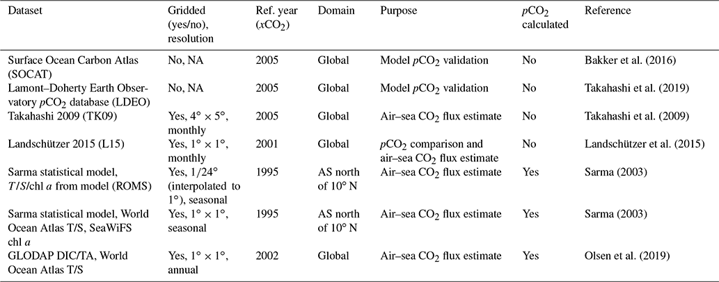
NA: not available
Alternative pCO2 products are used for comparison purposes. A complete list of these datasets and their characteristics is provided in Table 1. For all the comparison datasets, air–sea CO2 flux is calculated from monthly values. The ΔpCO2 values are calculated using Keeling curve data (downloaded from https://gml.noaa.gov/ccgg/trends/gl_data.html, downloaded 1 February 2022) of atmospheric xCO2 for the respective calibrated year of each dataset. The same climatological winds as used in the model (Sect. 2.2) are applied to the pCO2 products. The gridded product TK09 is chosen because previous modeling studies in the AS use it as validation (see “Introduction”). The L15 climatology, while based upon the same in situ data mentioned above, represents different processing methodologies and, as a high-resolution, global pCO2 dataset, also serves to provide independent context to the model validation. pCO2 is also calculated from DIC and TA provided by the statistical fits to JGOFS data by Sarma (2003) and to the gridded GLODAP climatological product. The statistical fits of Sarma (2003) are used twice, first using model SST, SSS, and chl a, and second with World Ocean Atlas (WOA) 2009 SST and SSS with SeaWiFS chl a. GLODAP-derived pCO2 also uses WOA 2009 SST and SSS applied to the annual DIC and TA values. Calculations of pCO2 are performed using the CO2SYS software package (Van Heuven et al., 2011). Since all calculations are conducted at the near surface, differences between this software suite and Orr and Epitalon (2015) are minimal. Furthermore, for air–sea CO2 flux intercomparison purposes, all pCO2 values except for TK09 are interpolated to the same 1∘ × 1∘ grid already shared by GLODAP, WOA, and L15. Due to the model's higher resolution, the re-gridding process reduces the area covered, consequently lowering the total model CO2 flux quoted in later sections of this study.
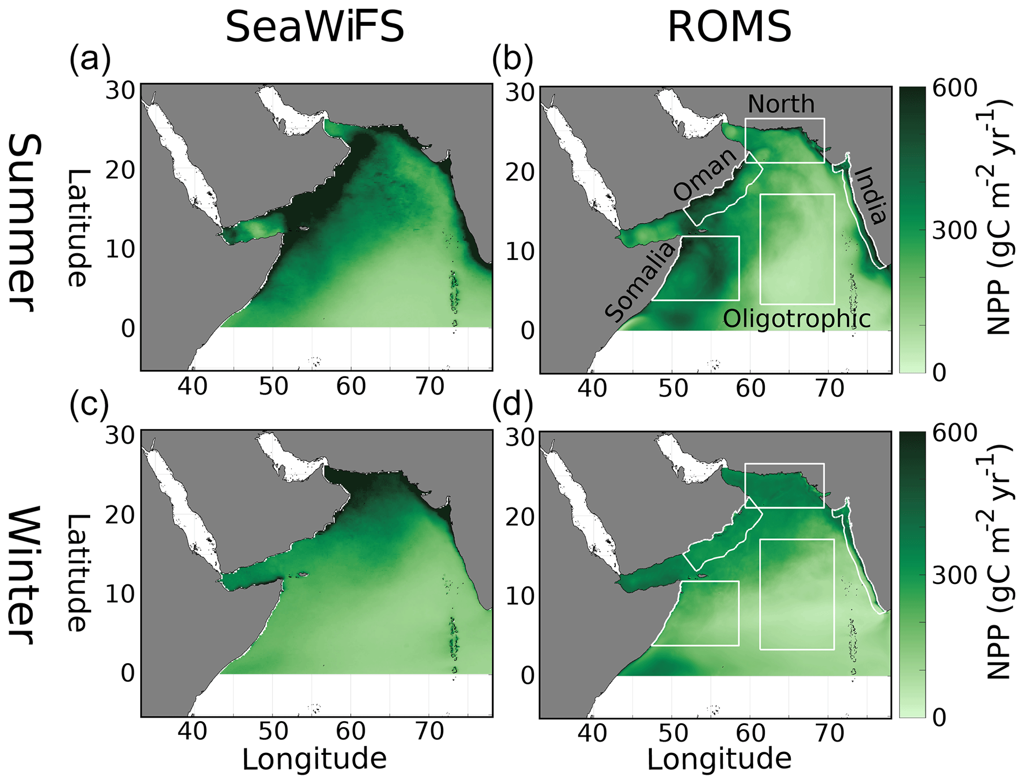
Figure 1Vertically integrated net primary production in the Arabian Sea () from the VGPM algorithm (Behrenfeld and Falkowski, 1997) for SeaWiFS data (years 1997–2010) (a, c) and model output (b, d) for summer (JJAS, a, b) and winter (DJFM, c, d) monsoons. White boxes in (b, d) denote regions of analysis in the paper.
2.2 Model details and setup
The model we use is the Regional Ocean Modeling System Adaptive Grid Refinement In Fortran (ROMS-AGRIF) version 3.1.1. (Shchepetkin and McWilliams, 2005). Previously used in the AS by Lachkar et al. (2016), the model is a free-surface primitive equation model, with a sigma and curvilinear grid for the vertical and horizontal dimensions, respectively. ROMS implements a forward–backward time-stepping algorithm with split baroclinic and barotropic modes. The advection of tracers uses a rotated-split third-order upstream biased algorithm to reduce spurious mixing (Marchesiello et al., 2009). The K-profile parameterization (KPP; Large et al., 1994) for vertical mixing is used. The model domain spans from 5.3∘ S to 30.5∘ N and from 33 to 78.1∘ E (Fig. 1). For the sake of comparison with Sarma et al. (2013), we will present the region north of the Equator and exclude the Red Sea and Arabian Gulf. The model's horizontal resolution is ∘, resulting in ∼ 5 km horizontal grid spacing.
Table 2List of parameters and their values used in the biogeochemical model.
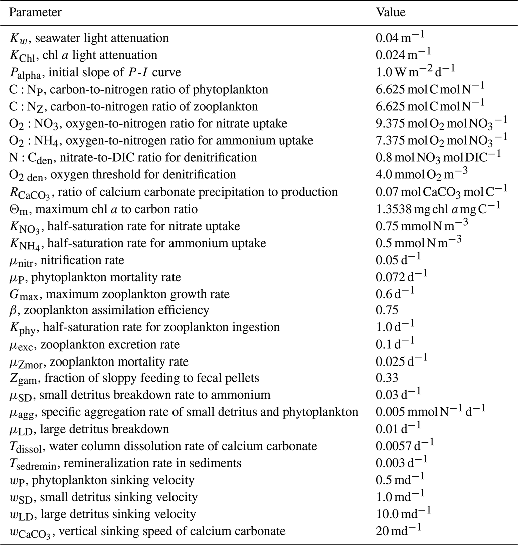
Coupled to the hydrodynamic model is a nitrogen-based biogeochemical model with two components for nutrients, nitrate and ammonium, with one phytoplankton, one zooplankton, and two detrital pools (Gruber et al., 2006). Biological parameters for the model are the same as those used in Gruber et al. (2011). A carbon module is also applied to the model with the state variables of DIC, TA, and calcium carbonate (CaCO3) (Gruber et al., 2012; Hauri et al., 2013; Lachkar and Gruber, 2013). In addition to the usual physical transport and mixing, CaCO3 is allowed to vertically sink at 20 m d−1. The chosen sinking rate is a simplification in that it does not include the faster rates observed for foraminifera shells (Curry et al., 1992), which as a biological group are not resolved by the biological model due to numerical constraints. Organic carbon is linked to organic nitrogen through the Redfield ratio 106:16. DIC is altered by air–sea CO2 flux, primary production, respiration, remineralization, and dissolution/precipitation of CaCO3. TA changes with the removal and creation of nitrate (NO3), including nitrification and denitrification, as well as dissolution/precipitation of CaCO3. The amount of CaCO3 precipitation is linked to primary production through a constant ratio of 0.07, meaning 0.07 moles of CaCO3 are produced for each mole of organic carbon. The dissolution rate is a constant 0.0057 d−1 in the water column and 0.002 d−1 in the sediments. Surface fluxes of DIC and TA due to evaporation, precipitation, and river input are included as virtual fluxes proportional to SSS forcing. Inside the module, surface carbon chemistry is calculated using routines from the Ocean Carbon-Cycle Model Intercomparison Project (OCMIP) carbonate chemistry routines (http://ocmip5.ipsl.jussieu.fr/OCMIP/phase3/simulations/, last access: 1 February 2022). Carbon chemistry coefficients used here include K1 and K2 CO2 dissociation from Millero (1995) and original data from Mehrbach et al. (1973) which was refit by Dickson and Millero (1987). A summary of the biological parameters used in the biogeochemical model is provided in Table 2.
The model is run with 360 d years and interpolated, climatologically averaged monthly forcing. The different climatological products derive from datasets spanning slightly different periods, and so here we assume that the dynamics represented within them have not changed in the time since. Heat flux, evaporation and precipitation, and restoring SSS are provided by the Comprehensive Ocean-Atmosphere Data Set (COADS; da Silva et al., 1994). SST forcing is provided by a monthly climatology of Pathfinder data from 1985 to 1997 (Casey and Cornillon, 1999). Wind stress is produced using the QuikSCAT/SCOW monthly climatology from 1999 to 2009 (Risien and Chelton, 2008). Tracer values for the initial conditions and the boundaries are given by WOA 2009 for temperature, salinity, NO3, and oxygen. Horizontal velocities u,v for initial and boundary conditions derive from the Simple Ocean Data Assimilation (SODA) analysis (Carton and Giese, 2008). Initial and boundary conditions for DIC and TA come from GLODAP from 300 m down to the bottom. Surface TA was calculated using the relations from Lee et al. (2006), and the corresponding DIC was calculated using WOA phosphate, silicate, T, and S values along with L15 pCO2. DIC and TA values between the surface and 300 m are calculated using density weighting. The model is spun up for 30 years, with 5 additional years for analysis. Atmospheric xCO2 values are set to 380 ppm, equivalent to 2005 levels, with an annual sinusoidal perturbation of 2.9 ppm.
2.3 Domains of analysis
In this study we focus on six distinct regions (Fig. 1). The first, the entire analysis domain, is the AS north of the Equator. The upwelling regions of the Omani and Somalian coasts are included separately to focus on the summer monsoon impact of enhanced DIC but also enhanced biological productivity (Schott and McCreary Jr, 2001). The Omani region begins at the coast and extends 300 km outward. The Somalian region begins near 3.8∘ N and extends north to the tip of the Horn of Africa, with an eastern extension to 58.6∘ E so as to encompass the region known as the Great Whirl (Vic et al., 2014), shown to be important for air–sea exchange in previous studies (Valsala and Murtugudde, 2015). The north region is defined by a rectangle from 21∘ N, 59.4∘ E to 26.5∘ N, 69.5∘ E, encompassing the northern part of the AS where the winter monsoon's primary productivity is most intense (Kumar et al., 2001). An oligotrophic region representing the central AS, which has less productivity and chlorophyll a on average (Fig. 1), is defined by a rectangle from 3.3∘ N, 61.31∘ E to 17∘ N, 70.8∘ E. The last region, covering the western coast of India, extends from the coastline 100 km offshore.
2.4 Analysis of air–sea CO2 flux, pCO2, and DIC variability
2.4.1 Air–sea CO2 variability
The air–sea flux in the model is calculated using
where K0 is the solubility determined by temperature and salinity (Weiss, 1974), α is the CO2 piston velocity with a quadratic wind speed dependence (Wanninkhof, 1992), and the difference in ocean and atmosphere pCO2, ΔpCO2, is arranged so that the flux convention is positive outward from the ocean. The choice of Wanninkhof (1992) for the solubility parameterization is for direct comparison with previous modeling studies (see “Introduction”), despite the fact that more recent formulations are available, such as Wanninkhof (2014). The objective being to characterize seasonal anomalies of air–sea CO2 flux, here we use a Reynolds decomposition. Briefly, a Reynolds decomposition takes a time series and divides it into a temporal mean and fluctuating component. When applied correctly, multiple terms can be produced in isolation showing their fluctuating contribution to the total. Noting that temperature effects upon solubility (K0) and piston velocity (α) approximately cancel, meaning that their product mostly reflects wind forcing, we have the following arrangement for the decomposition of flux anomalies (Doney et al., 2009b):
where ′ indicates an anomaly and is a 5-year average of variable x, which are calculated at each grid point. The 5-year average is necessary for exact closure in the Reynolds decomposition. is the seasonal flux anomaly, with groupings based on wind anomalies (K0α)′, anomalies, and cross-terms involving both.
The winds in this study are prescribed, so uncertainty in air–sea flux stems from pCO2. The SOCAT protocol assigns a minimum uncertainty of 2 µatm to observations. Using the average SST and SSS from the SOCAT observations, the solubility change is 2.68 × 10⁻² . Wind speeds of 1, 5, and 10 m s−1 will then produce a shift of 0.0018, 0.0443, and 0.177 , respectively. The model presents a median value of 1.28 with median winds of 5 m s−1, so therefore the baseline uncertainty in air–sea CO2 is ∼ 3.5 %.
2.4.2 pCO2 variability
The proximate variables that affect pCO2 change in the model are DIC, TA, SST, and SSS. Following previous studies (Lovenduski et al., 2007; Turi et al., 2014), we use a first-order Taylor expansion to decompose pCO2 into contributions from these four, neglecting contributions from nutrients (phosphate and silicate). Initially, the decomposition would follow the form
where ΔpCO2 is the perturbation of pCO2 from a mean value, and the Δ terms for DIC, TA, SST, and SSS likewise express deviations from a prescribed value depending on whether the deviations are spatial or temporal in nature (see below). The coefficients of the Δ terms are partial derivatives of pCO2 with respect to these variables, namely DIC, TA, SST, and SSS, and are calculated via centered differences described below. However, in order to control for salinity effects on DIC and TA (Keeling et al., 2004), we normalize DIC and TA by the salinity S0 = 35 psu to create the variables
Substituting these terms into Eq. (3), we can expand to produce, for example with DIC, the following (Lovenduski et al., 2007):
Collectively, the ΔSSS term in Eq. (5) and its counterpart in TA can be added to the original ΔSSS term in Eq. (3) to represent all salinity effects in a “freshwater” term so that we now have the following (Turi et al., 2014):
For the remainder of this paper, when discussing the results of the Taylor series decomposition method, it will be understood that DIC and TA refer to DICs and TAs, and SSS will refer to the combined term.
The contributions of DIC, TA, SST, and SSS to pCO2 variability are used to construct maps and time series of pCO2 anomalies. In order to calculate the anomaly, ΔpCO2 requires calculating both the Δ deviations of DIC, TA, T, and SSS, as well as partial derivatives. In this study, we calculate both temporal and spatial anomalies. To consider spatial variability, starting with annual means of pCO2, DIC, TA, SST, and SSS, an average value for the whole domain is calculated and removed from each grid point's annual mean to get a Δ perturbation or anomaly. Similarly, for temporal variability, with the monthly values of pCO2, DIC, TA, SST, and SSS at each grid point, the annual average at that grid point is removed to produce the monthly Δ perturbation/anomaly. Partial derivatives are approximated via centered differences. These are obtained by calculating pCO2 with slight deviations of DIC, TA, SST, and SSS from the mean value. Both positive and negative deviations are used to construct centered differences, with deviation magnitude determined by Orr et al. (2018). For example to calculate the monthly pCO2 anomaly due to SST for a grid point with annual mean pCO2 of 430 µatm, annual mean SST of 24 ∘C, and monthly SST of 26 ∘C, the following equation is used:
where 1 × 10⁻⁴ is the recommended SST deviation.
2.4.3 DIC budget
Whereas the state variables of DIC, TA, SST, and SSS provide the chemical context which determines carbon availability to potential air–sea flux via pCO2, tracking the overall inventory of inorganic carbon (i.e., DIC) allows for the parsing of numerous source and sink processes governing the total amount of carbon reaching the surface. Beyond the biological processes impacting DIC as outlined in Sect. 2.2, the physical processes impacting DIC are air–sea CO2 flux, surface evaporation and precipitation, horizontal and vertical advection, and horizontal and vertical mixing. In order to diagnose the relative importance of these terms (i.e., to weigh competition between upwelling circulation source and biological drawdown sink), we calculate the budget IDIC in a 3D volume by integrating
with
which is the volume-specific flux J of DIC in a given grid cell. PPNew+Reg is net community primary production scaled by the Redfield ratio, is net CaCO3 precipitation and remineralization, Zooresp is zooplankton respiration, and Detremin is remineralization of both detrital pools. All these terms are grouped together into “Biology” because they represent all biological processes. FAS is air–sea flux, with a sign convention of positive outward. Advx is advective flux in the x direction, with corresponding y and z components. Mixx is the x component of mixing flux, again with y and z components. All x and y components of both advective and mixing DIC fluxes are grouped into horizontal circulation, with a similar grouping for vertical circulation in the z direction. Evap-Precip is the forced virtual flux from evaporation and precipitation at the surface. A is the two-dimensional horizontal area to be considered, which in our study includes the entire domain but also the subregions of analysis. The bottom boundary of integration, −z(σ), is the sigma-layer depth at which integration starts, moving up to the free-moving surface η. We chose to integrate the top five sigma layers of the model, corresponding to ∼ 20 m depth. This level was chosen because below this depth, annual cycles of IDIC begin to deviate from the surface DIC, which is our focus in this study of air–sea CO2 flux.
3.1 Model validation and pCO2 data-model comparisons
The implementation of ROMS-AGRIF presented here has been used in previous studies of the AS (Lachkar et al., 2016). Model output of net primary productivity (NPP) captures the summer monsoon highs near the upwelling regions of Oman and Somalia (model > 400 vs. data > 500 ), with enhanced NPP in the north during the winter monsoon (model ∼ 300 vs. data > 400 ) (Fig. 1). The model also captures the vertical distributions of temperature and salinity (Figs. S1 and S2 in the Supplement) with deviations from WOA around 1 oC and 0.2 psu. Depth profiles of nitrate, oxygen, DIC, and TA are similarly conserved (Figs. S3–S6 in the Supplement). Nitrate, DIC, and TA all show their usual nutrient-like profiles, while oxygen is its minimum within the OMZ. The deviations seen between in situ data and model output are greatest at depths less than 500 m. Deviations in near-surface NO3 (Fig. S3) can be large for intermediate values (5–20 µM) but overall do not show a systematic bias. DIC (Fig. S5) also has large deviations (∼ 50 µM) in the top 500 m and with a slight positive bias. It is in TA (Fig. S6) that deviations, while similarly ∼ 50 µM eq, show a consistent near-surface underestimation. The surface currents in the model also demonstrate the monsoonal shifts and reversals seen in the AS (Fig. S7 in the Supplement).
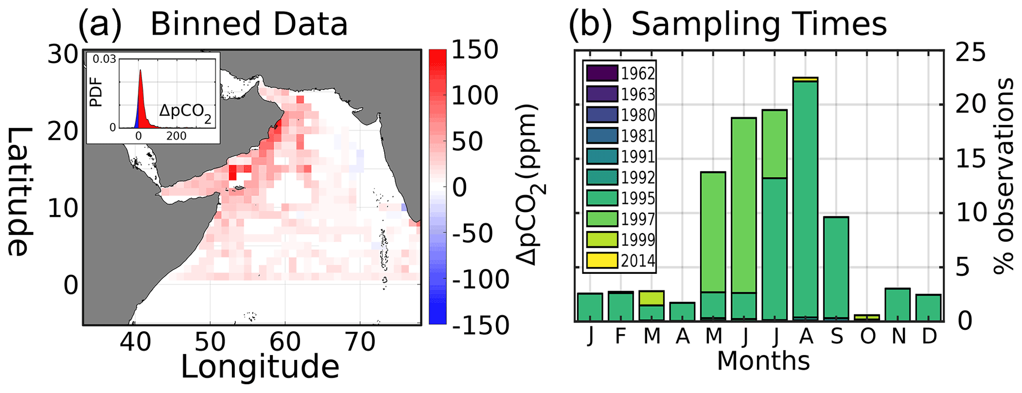
Figure 2(a) Average surface in situ ΔpCO2 (ppm), with probability density function of all ΔpCO2 values inset. ΔpCO2 data are calculated in comparison to Keeling atmospheric pCO2 and then binned into a 1∘ × 1∘ grid. (b) Monthly distribution of in situ data sampling times, color-coded by sampling year.
Regarding pCO2, in situ data from the merged SOCAT–LDEO database show that ∼ 90 % of ΔpCO2 values in the AS are positive (Fig. 2a, inset), indicating a positive flux to the atmosphere that is applicable geographically (Fig. 2a). Sampling dates for pCO2 (Fig. 2b) show that ∼ 70 % are from the summer monsoon months (June–September, JJAS). Most observations similarly date from the 1990s, with 1995 and 1997 alone accounting for 96 %.
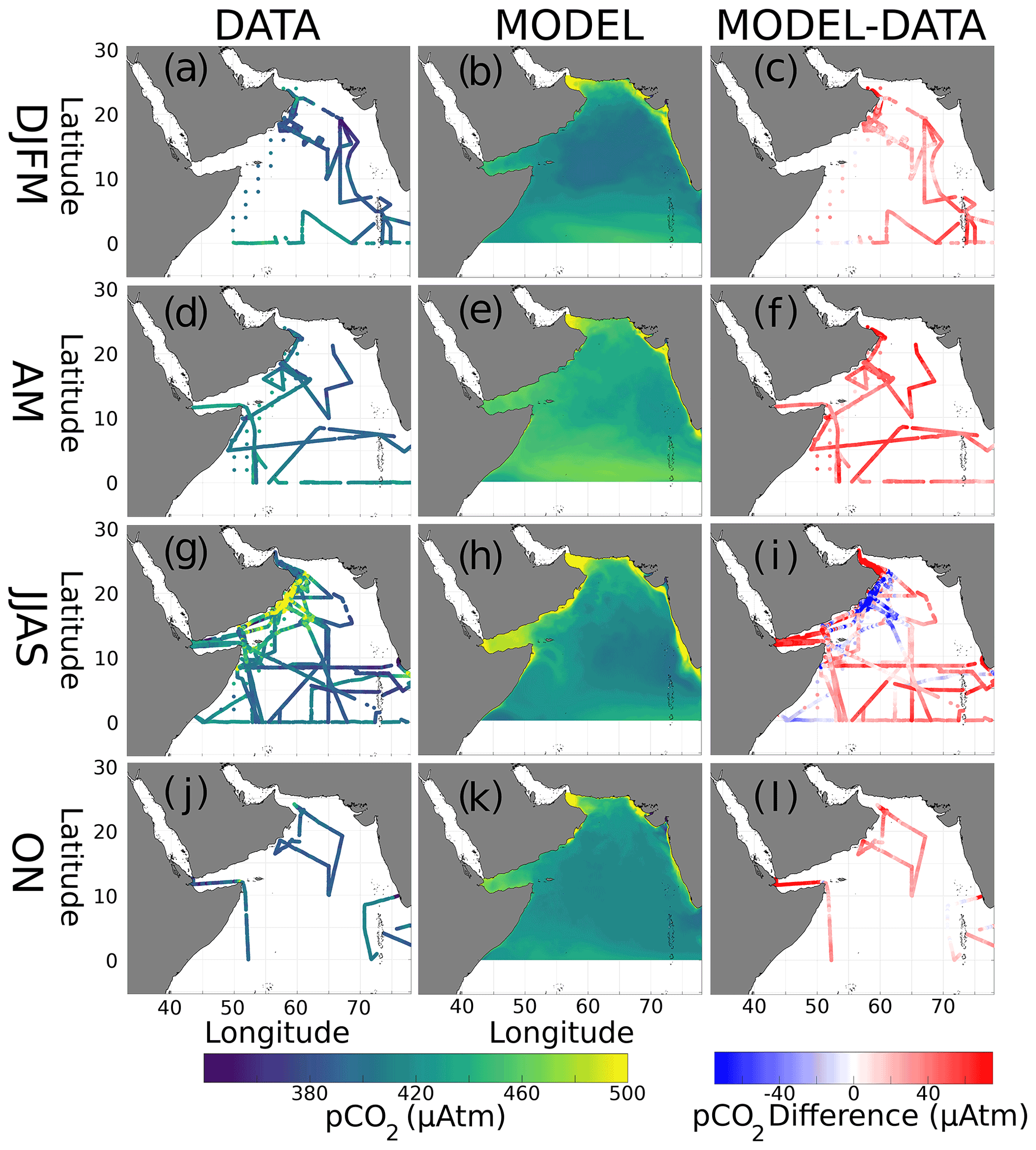
Figure 3Seasonal surface pCO2 (µatm) from data (left column, a, d, g, j) and the model (middle, b, e, h, k), as well as their differences (right, c, f, i, l). Plots are arranged by season: winter monsoon (DJFM, a–c), spring intermonsoon (AM, d–f), summer monsoon (JJAS, g–i), and fall intermonsoon (ON, j–l).
Table 3Mean and standard deviation (in parentheses) of annual and seasonal surface pCO2 (µatm) in both the merged dataset and model.
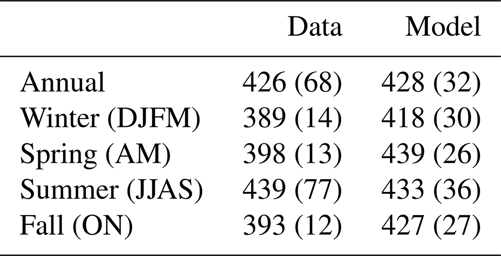
Seasonal pCO2 distributions from both data and the model are shown in Fig. 3. During the winter monsoon, pCO2 values are at their lowest (range: 348–455 µatm; Fig. 3a). The spring intermonsoon (Fig. 3d) finds pCO2 values similar to the winter (range: 354–451 µatm), with data coverage improving in the western AS. The summer monsoon, with the best data coverage (Fig. 3g), has pCO2 peaking at 773 µatm. In contrast, the fall intermonsoon (Fig. 3j) has very little data coverage, with pCO2 ranging from 311 to 485 µatm. Similar to the data, model pCO2 (Fig. 3b) is at its lowest during the winter. However, in the spring (Fig. 3e) open-ocean pCO2 finds its peak with a domain average of 439 µatm, which is not reflected in the in situ dataset (Fig. 3d and e). Maximum model pCO2 is found in the summer monsoon near upwelling regions (Fig. 3h), with values attaining > 800 µatm in Oman. Fall model pCO2 (Fig. 3k) still has elevated values averaging 427 µatm but less than the summer period. Certain regions in the model show persistent maxima in pCO2, such as the Gulf of Oman and the Strait of Hormuz, which are not reflected in the few data collected there. Model pCO2 values in the Gulf of Aden increase during spring and then peak during the summer, a pattern which is unclear from the data. Annual and seasonal pCO2 means, with standard deviations in parentheses, are displayed in Table 3 for both the data and model. Differences from interpolated model output and in situ data are shown on the right column of Fig. 3 (Fig. 3c, f, i, and l). Most differences show that model output is higher in value than the data, averaging 24.6, 48.4, and 33.7 µatm higher for the winter, spring, and fall seasons, respectively.

Figure 4Taylor diagram of modeled vs. observed surface pCO2, both annually and seasonally. Data are from merged SOCAT and LDEO databases, corrected to the year 2005. Distance from origin (concentric solid lines) is normalized model standard deviation. Angle from vertical axis is Pearson correlation coefficient. Distance from observation point (black dot) is root-mean square deviation (dashed blue lines). Color of each point denotes model bias; i.e., positive values are overestimates.
A Taylor diagram (Taylor, 2001) comparing in situ pCO2 data with model output shows the model's relative performance (Fig. 4). The distance from the origin is model variability normalized by standard deviation of the in situ data. The angle created from the y axis is the Pearson correlation coefficient between the model and in situ data. If the model were to perfectly reproduce the data, it would appear at the position (1,0), equivalent to a normalized standard deviation of 1 and correlation coefficient of 1. For the entire dataset, as well as for the spring and summer seasons, the model's correlation with data is ∼ 0.5. Winter and fall have lower values at 0.2 and 0.06, respectively. Variability expressed as normalized standard deviation shows that overall, and during spring and summer periods, the model underestimates data variability (∼ 0.5 µatm). During the winter and fall, however, the model overestimates variability (1.1 and 1.6, respectively). For all periods apart from summer, model pCO2 has a positive bias (9.1, 24.6, 48.4, and 33.7 µatm for the annual, winter, spring, and fall, respectively). During the summer, the model has a negative bias of −3.1 µatm.
The source of bias in pCO2 is linked to the four state variables SST, SSS, DIC, and TA. Comparisons with the model are made with SST and SSS from the merged SOCAT–LDEO database, while DIC and TA come from the ungridded GLODAP product (Fig. S8 in the Supplement). In this case, model SST and SSS (Fig. S8a and b) largely overlap with a 1:1 relationship but with slight positive biases of ∼ 0.4 oC and 0.3 psu. Removing these biases from the model results in a pCO2 shift of −6.8 and −3.5 µatm for SST and SSS, respectively. These deviations are close in magnitude to the best-case measurement error of ∼ 2 µatm. Taylor diagrams for SST and SSS (Fig. S9 in the Supplement) further show the seasonal performance of these two variables. The model performs best for SST (Fig. S9a) during the winter, with a correlation of 0.93 and a normalized standard deviation of 0.97. The other seasons have lower correlations (0.74–0.81) and reduced standard deviations (0.63–0.8) except for the fall with a standard deviation of 1. SSS (Fig. S9b) has lower correlations and standard deviations than SST, with all seasons demonstrating a positive bias (0.02–0.39 psu). Correlation is best in the winter at 0.89 and worst in the fall at 0.46. Model variability in SSS is also less than the data, with standard deviations ranging from 0.33 to 0.72. Lower variability is most likely due to the raw nature of the in situ data used here, in opposition to the monthly averaged climatological forcing and initial conditions of the model.
Ungridded DIC and TA data from GLODAP, though more sparse (n=334 data points with both DIC and TA at depths ≤ 50 m), show more deviation from the 1:1 line (Fig. S8c and d) with overall negative biases of −15.8 µmol kg−1 and −30.0 µmol eq kg−1 for DIC and TA. These biases result in pCO2 perturbations of −33.8 and +45.7 µatm, respectively, when accounted for individually. Since the buffering capacity of seawater is related to the ratio of TA and DIC, when both biases are considered, average pCO2 shifts +16.7 µatm. As a result, while the DIC model bias lowers pCO2, the stronger bias in TA is the most likely cause for the model's overall positive pCO2 bias, which may in part be due to the unresolved fast sinking rates of foraminifera in the model.
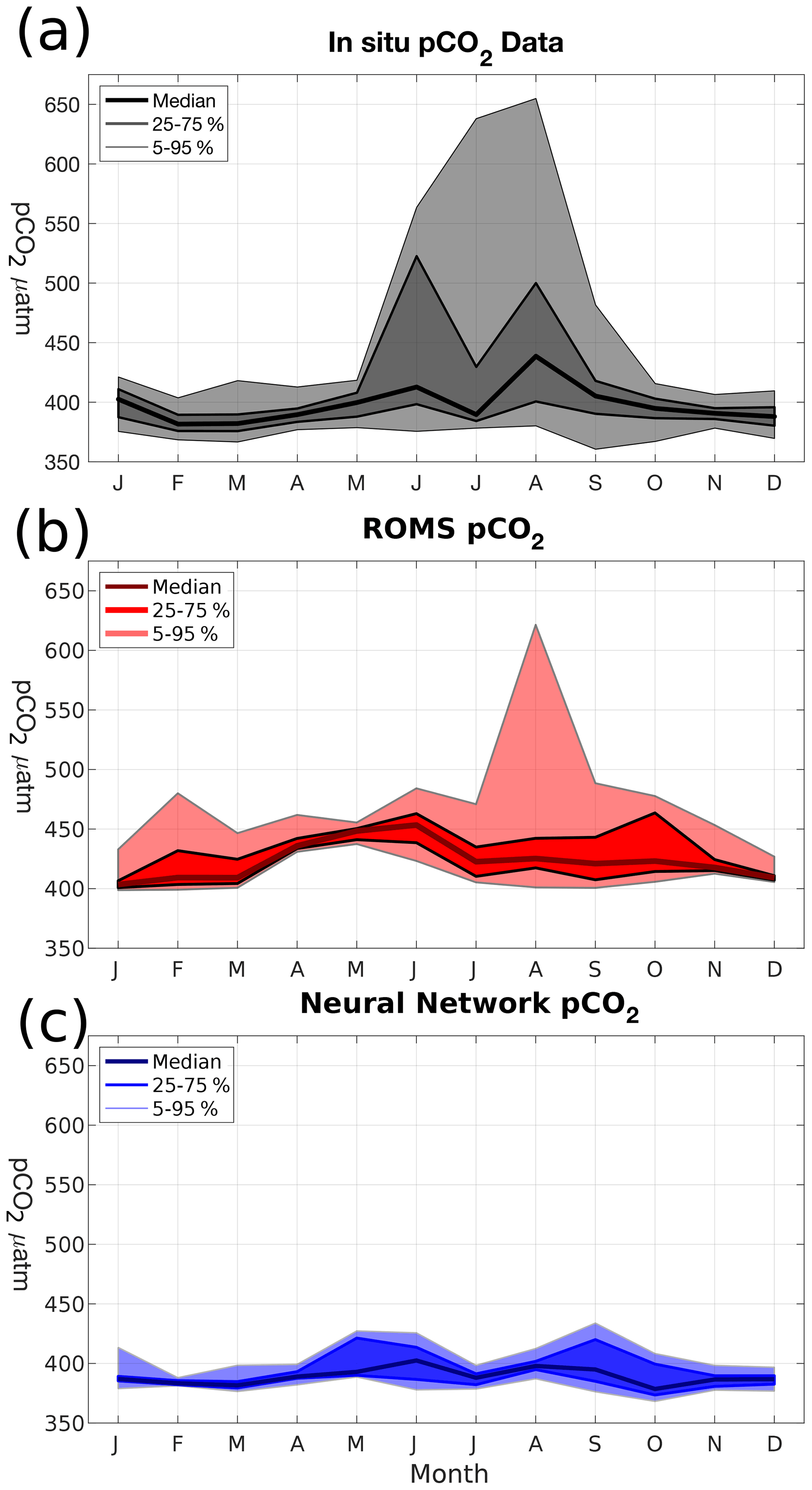
Figure 5Monthly probability density distributions of surface pCO2 (µatm) in (a) merged SOCAT–LDEO in situ data, (b) modeled pCO2, and (c) L15 pCO2 climatology.
Direct comparisons between the in situ and model output demonstrate the positive bias and middling correlations of the model with respect to the data, as well as the model's tendency to underrepresent variability. As a result, it is necessary to investigate how these shortcomings compare with alternative pCO2 estimates in the AS. Figure 5 shows monthly comparisons of the pCO2 probability distribution functions from in situ data, model output, and L15. For most of the year, the data (Fig. 5a) stays within a relatively narrow range (375–425 µatm) except for the summer monsoon when values can exceed 500 µatm and the median value has its peak. In the model (Fig. 5b), pCO2 is almost entirely above 400 µatm, with the median value increasing during the spring intermonsoon and peaking in June (453 µatm). Similar to the data, the upper-bound variability in pCO2 peaks in August. L15 (Fig. 5c), by contrast, has a tighter envelope of variability, with 5–95 percentile values never going beyond the range of 368–434 µatm. Median pCO2 in L15 peaks in the summer like the data at 402 µatm, but there is no large increase in upper-bound variability, with the 95 % upper bound in L15 reaching 434 µatm in September.
In summary, the survey of available data and comparing it to the model output produces a few distinct features: (1) available in situ data show that the majority of observations are skewed towards the summer monsoon during the years 1995 and 1997; (2) most in situ data show CO2 out-gassing in the AS; (3) the model has a net positive bias in surface pCO2, driven by a joint DIC-TA bias which is slightly stronger in TA; and (4) the model captures the high summer monsoon pCO2 values better than the alternative L15 climatology.
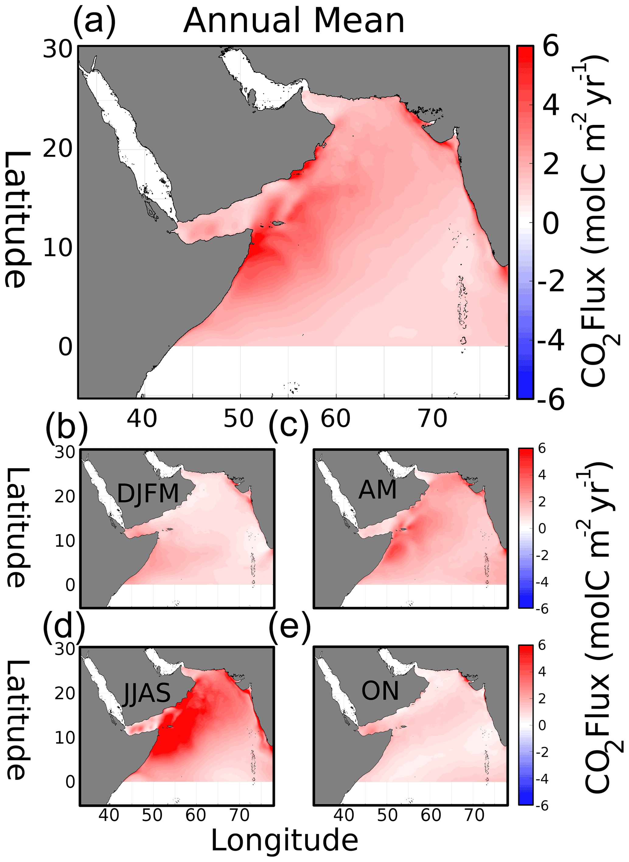
Figure 6(a) Modeled annual mean air–sea CO2 flux density (). (b–e) Seasonal flux density for winter (DJFM), spring (AM), summer (JJAS), and fall (ON), respectively. Positive is flux out of the ocean.
3.2 Air–sea CO2 flux, drivers of seasonal variability, and flux intercomparison
Modeled annual mean atmospheric flux of CO2 (Fig. 6a) shows outgassing (positive, red) throughout the entire domain, producing an average annual CO2 flux density rate of 1.9 and a total of 162.6 Tg C yr−1. Similar to pCO2, several hotspots appear in the geographic distribution. Near the coast of Oman, the average flux density is 2.7, with 3.2 in Somalia and 2.4 along the coast of India, producing a flux of 11.4, 32.9, and 4.9 Tg C yr−1, respectively. The other regions, the north AS and oligotrophic central AS, have average densities of 2.0 and 1.5 , with total fluxes of 10.5 and 28.6 Tg C yr−1. The seasonal air–sea flux (Fig. 6b–e) has minima during fall and winter, with an increase in spring and a strong maximum during the summer monsoon. Omani and Somalian flux densities during the summer monsoon are 5.8 and 5.9 , respectively. The distribution of enhanced summer air–sea CO2 flux coincides with the southwest monsoon winds (Fig. S10 in the Supplement), as well as the band of cooler temperatures impacting spatial pCO2 anomalies (see Sect. 3.3.1). The entire domain fluxes of 32.0, 26.6, 90.9, and 13.1 Tg C yr−1 for the winter, spring, summer, and fall periods, respectively, each contribute 19.7, 16.3, 55.9, and 8.1 % of the annual total.
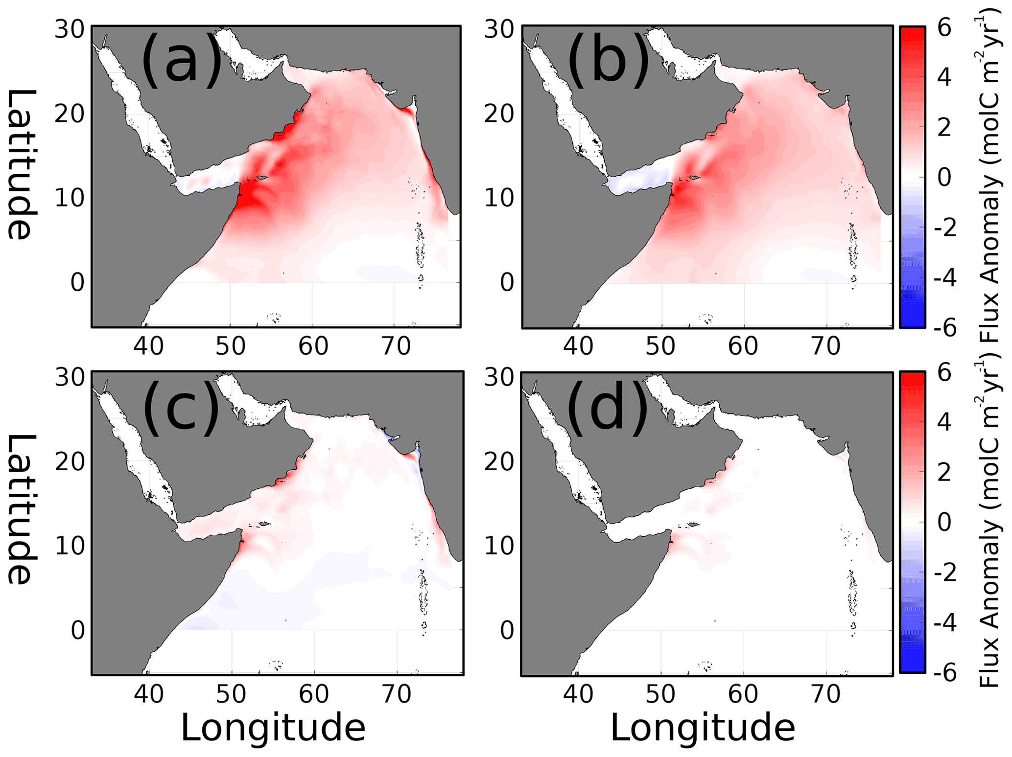
Figure 7(a) Anomaly of air–sea CO2 flux during the summer monsoon (JJAS; ). Summer flux anomaly contributions due to (b) wind, (c) pCO2, and (d) cross-terms in Eq. (2).
The variability in air–sea CO2 flux can be attributed to the contributions of winds, ΔpCO2, and interacting cross-terms, as described in Eq. (2). The temporal anomalies for the summer monsoon, the period with the strongest CO2 flux signal, are presented in Fig. 7. Most of the domain has positive but variable strength anomalies in air–sea flux (Fig. 7a), averaging 1.3 with a standard deviation of 1.35. The wind contribution to flux variability, κα (Fig. 7b), is also positive in most of the domain except the Gulf of Aden and the southeastern corner of the domain. The wind anomaly's magnitude and distribution closely match the total anomaly in Fig. 7a, with a mean flux anomaly of 1.18 and 0.96 standard deviation. The ΔpCO2 contribution to seasonal flux anomaly (Fig. 7c) has a lower-magnitude effect overall (mean flux anomaly 0.1, deviation 0.5, maximum 6.2 ), with positive values north of 10∘ N and slightly negative to the south. The maxima approaching 6.2 are in the upwelling centers of Oman, Somalia, and the Indian coast. Second-order cross-term values (Fig. 7d) are almost all positive, with maxima also occurring near upwelling centers similar to the ΔpCO2 term but weaker in magnitude with an average of 0.04 .
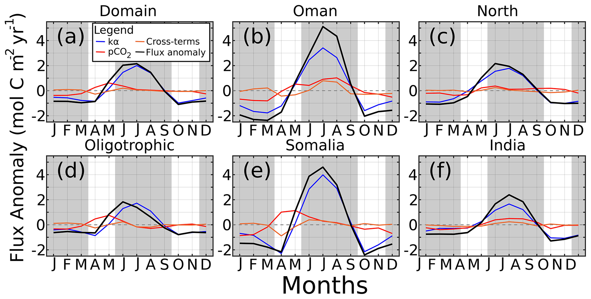
Figure 8Monthly CO2 air–sea flux anomaly () for (a) the domain, (b) Oman, (c) north AS, (d) oligotrophic central AS, (e) Somali coast, and (f) Indian coast. Contributors to the flux are solubility and winds (kα, blue), pCO2 (red), and cross-terms (orange). Gray regions indicate winter and summer monsoons.
The seasonal flux anomalies for all regions are displayed in Fig. 8. The summer monsoon flux is so strong that it makes the anomalies (black lines) for all the other seasons negative except for May in the spring. During the winter months (DJFM), both wind and pCO2 terms produce negative flux anomalies (ranging to −0.78 and −0.38 in the domain for wind and pCO2, respectively; Fig. 8a), indicating the relative lack of winds and minimum pCO2 values. In winter, while the negative wind term is universally strongest, within the upwelling regions the pCO2 term is 58 % (Fig. 8b) of the wind term's magnitude, and 49 % for the entire domain. The spring intermonsoon, where many regions such as Somalia and the central oligotrophic AS (Fig. 8d and e) experience their pCO2 maximum, shows a positive pCO2 effect on flux anomaly that is as large as or larger than the negative wind effect (Somalian May pCO2 anomaly of 1.1 , wind anomaly of 0.1). Summer monsoon winds represent the majority contribution to CO2 flux variability, with a minimum 64.7 % contribution relative to the total anomaly in India, a maximum of 112.8 % in the oligotrophic AS, and 90.8 % for the whole domain. By contrast, summer pCO2 and cross-terms contribute 6.0 % and 3.1 % to the domain's anomaly, respectively. Fall intermonsoon months resemble the winter monsoon, with negative wind anomalies contributing most with small or negative pCO2 contributions. In most scenarios, pCO2 contributes in the same direction as the winds or little at all, with the notable exceptions of Oman, oligotrophic AS, Somalia, and the domain during spring intermonsoon.
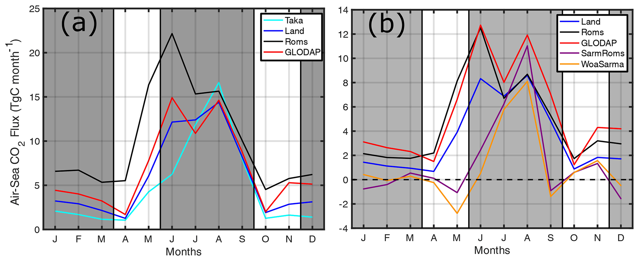
Figure 9(a) Monthly CO2 flux (Tg C month−1) from the AS as calculated using pCO2 from TK09 (cyan), L15 (blue), model (black), and GLODAP (red). (b) Monthly CO2 flux from 10∘ N and north using pCO2 from L15 (blue), model (black), GLODAP (red), Sarma using model output (purple), and Sarma using WOA data (orange). Dashed line in (b) is the zero flux axis, and gray regions denote winter and summer monsoons. Positive flux is out from the ocean surface.
While strong monsoon winds dominate the timing of air–sea CO2 flux, and the AS is always a source of CO2 due to positive ΔpCO2, differences in pCO2 between independent sources can still result in a wide range of overall magnitudes. In the AS, CO2 outgassing estimates vary from 7 Tg C yr−1 (Goyet et al., 1998b) to > 90 Tg C yr−1 (Sarma, 2003) and everything in between (Somasundar et al., 1990), with each study using their own pCO2 data and wind parameterizations. Considering the important seasonal role of winds, the best way to investigate the role of pCO2 variability is to keep winds (and their flux parameterization) constant. Towards this end, we use multiple pCO2 products to calculate CO2 flux with the same wind and parameterization as the model (Fig. 9). As summarized in Table 1, pCO2 from TK09, L15, GLODAP data, and Sarma (2003), interpolated to the WOA 1∘ × 1∘ grid, is used in these calculations (except for TK09 in which the coarse resolution reduced coverage). The original applicability of the Sarma (2003) model is north of 10∘ N, and so flux is calculated for this region, as well.
All calculations have their peak CO2 flux sometime in the summer, confirming the role of winds in CO2 flux timing. This study's model consistently produces one of the higher estimates with 120 Tg C yr−1 (reduced from 162.6 due to re-gridding) and 57 Tg C yr−1 north of 10∘ N. The only estimate higher than the model is GLODAP data in the region north of 10∘ N with 65 Tg C yr−1 possibly driven by summer monsoon sampling bias. The high model estimate is perhaps unsurprising, considering the pCO2 bias. The range in estimates of total CO2 flux is 57–120 Tg C yr−1, resulting in a ratio of 2.1× variability. In the reduced domain of the AS north of 10∘ N, estimates range from 12.3 to 65.6, resulting in 5.3× variability. The 5.3× ratio is quite high and is in part driven by the low estimates from the Sarma (2003) model, which are 12.3 and 17.6 using tracer data from WOA and ROMS, respectively. Indeed, the Sarma (2003) model estimates have negative CO2 flux for some months, which is not observed in the original publication, and the total fluxes are quite smaller than the 70 Tg C yr−1 reported. If the two lower estimates are removed, the range in air–sea CO2 flux in the domain north of 10∘ N is 41–65 Tg C yr−1, providing a ratio of 1.6 similar to 2.1 for the whole domain. Even considering the model's pCO2 bias, as previously mentioned the GLODAP estimate supersedes it in the region north of 10∘ N, as does the original Sarma (2003) estimate of 70 Tg C yr−1. Thus, while we may think the model overestimates flux, it is still within the range of previous studies in the AS.

Figure 10(a) Spatial anomaly of time-averaged surface pCO2 (µatm). Black boxes represent regions of analysis used in (b) to show averaged contributions of four parameters to pCO2 variability. The changes in pCO2 due to these variables are shown for (c) temperature, (d) DIC, (e) TA, and (f) SSS.
3.3 The pCO2 distribution, seasonal cycle, and underlying contributors
3.3.1 Spatial pCO2 distribution
Spatial pCO2 anomalies calculated from the annual mean highlight the geographic hotspots of pCO2 inside the domain (Fig. 10a). The pCO2 anomalies range from −89 to +415 µatm, indicative of a positive skew in the distribution. Within the regions of analysis prescribed in this study, it is clear that Oman, the Indian coast, and the north AS host enhanced pCO2, with average positive anomalies of 8.6, 21.5, and 49 µatm, respectively. In contrast, both the oligotrophic central AS and Somalian regions have negative pCO2 anomalies (−13.7 and −2.9 µatm, respectively). The contributing factors to these pCO2 anomalies, SST, DIC, TA, and SSS, display differing distributions. SST (Fig. 10c) contributes toward negative pCO2 anomalies in a southwest-to-northeast band along the coasts of east Africa and the Arabian peninsula, up to the coasts of Pakistan and the northern coast of India near Gujarat. The cold SST structure contributes a −20 µatm effect on pCO2 and largely overlaps the stronger summer monsoon winds (Fig. S10). The opposite trend is found in the central oligotrophic and Indian regions, where the average temperature contribution to pCO2 is 20 µatm despite upwelling along the southern Indian coast. The distribution of DIC-induced anomalies (Fig. 10d) shows a positive influence near coastal regions and the western AS off the coast of Somalia (+25 µatm), whereas a strong minimum is found in an oval region encompassing the central, open-ocean AS (−36.6 µatm). TA effects (Fig. 10e) show a north–south gradient similar to SSS, with positive contributions to pCO2 of +20 µatm occurring in the north and −20 µatm towards the south, resulting in magnitudes similar to SST contributions. SSS contributions (Fig. 10f) show a similar distribution as TA but are weaker in magnitude (± 10 µatm).
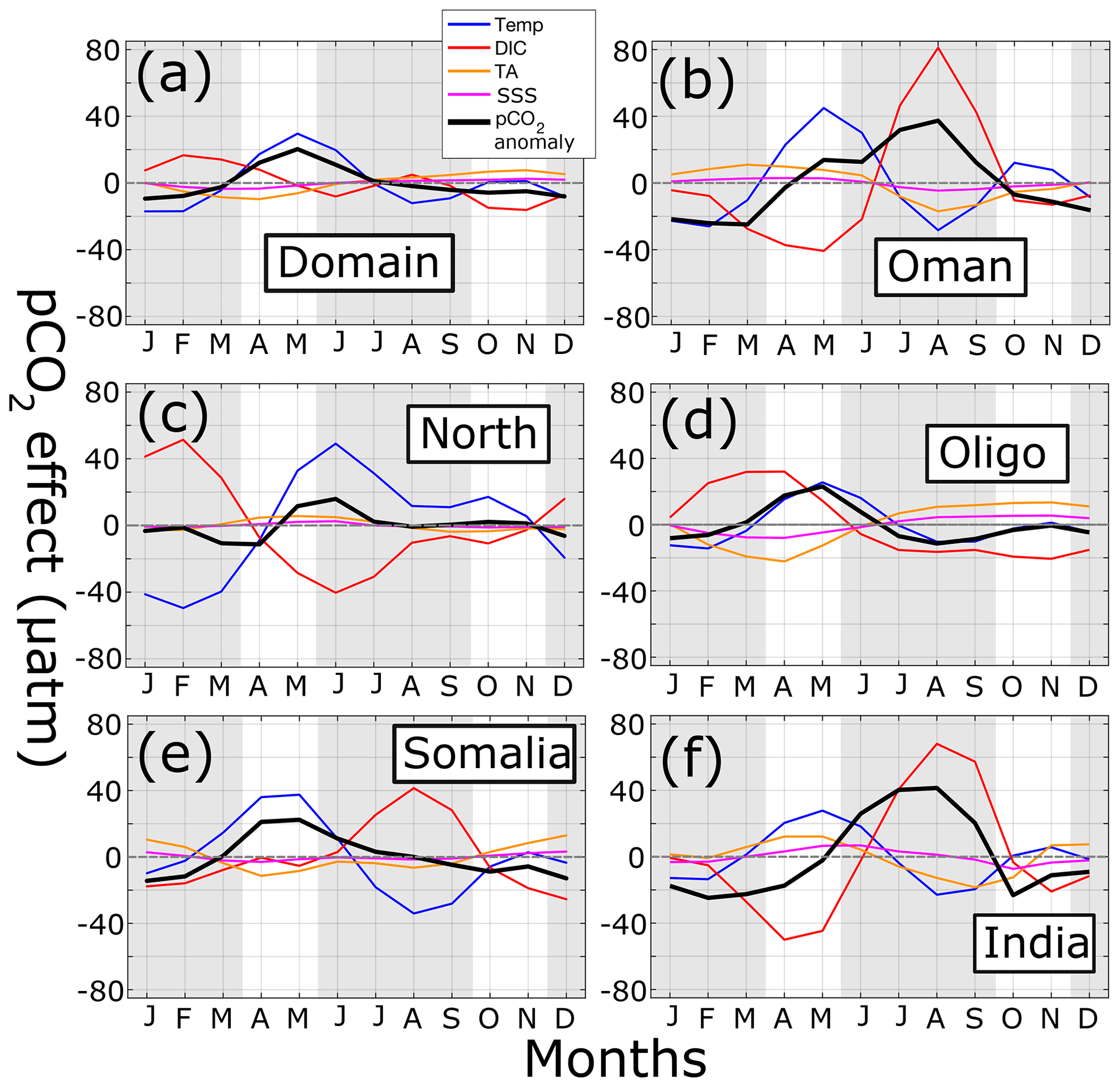
Figure 11Time series of pCO2 anomalies (µatm) (black lines) for (a) the entire domain, (b) Oman, (c) north AS, (d) oligotrophic central AS, (e) Somalia, and (f) India. Dashed gray lines indicate horizontal axis. Gray shading shows summer and winter monsoons. Additional lines show change in pCO2 due to temperature (blue), DIC (red), TA (orange), and SSS (magenta).
3.3.2 Seasonal pCO2 cycle
The previous section outlines the geographic regions within the AS that have overall high or low pCO2 values, but in order to investigate the strong seasonal monsoon cycle in the AS, the decomposition of variables affecting monthly pCO2 values is calculated at each model grid point and averaged into each analysis region (Fig. 11). Regarding the whole domain (Fig. 11a), pCO2 variability is similar to that seen in Fig. 5b, with a spring pCO2 anomaly peak (20 µatm) and minimum during fall and winter (−9.4 µatm). Temperature effects largely mirror the overall pCO2 cycle (May peak 30 µatm, January minimum −17 µatm). Change in pCO2 associated with DIC acts in opposition to temperature but with lower magnitude (16 µatm in February, −8 µatm in June). Both TA and SSS effects are negative for the first half of the year before becoming slightly positive in the second half, never reaching 10 µatm in magnitude.
Different pCO2 anomaly cycles can be found in the upwelling regions of Oman, Somalia, and India (Fig. 11b, e, and f). Here, a positive temperature peak appears in the spring (27–45 µatm), which is then supplanted by a positive DIC peak during the summer monsoon (41–81 µatm). In both Oman and India, the summertime DIC peak is strong enough to contribute to the annual pCO2 peak despite cooler temperatures. In Somalia, the summertime DIC peak is not sufficiently stronger than temperature (41 vs. −34 µatm) such that in sum with the other terms maximum pCO2 is found in the spring, not the summer, similar to the whole domain and oligotrophic regions. Both TA and SSS effects in these three regions are lower in magnitude (never exceeding 18.4 and 7.3 µatm for TA and SSS, respectively) and generally run counter to DIC.
A completely different regime occurs in the north AS (Fig. 11c). Here, while temperature effects (49 µatm in June) create a similar spring–summertime peak in pCO2 (15.9 µatm) somewhat counteracted by DIC (−40 µatm), during the winter monsoon temperature and DIC effects are both maximal and in opposing amplitudes (−49.5 and 51.4 µatm for SST and DIC, respectively). This occurs due to the convective mixing that occurs during winter in the north AS, where cooling temperatures lower pCO2, but subsurface water introduces more DIC, resulting in a near-balance.
The oligotrophic central region (Fig. 11d), the largest in area, has similar pCO2 and temperature impacts as the whole domain, with the two largely overlapping. DIC, TA, and SSS impacts also follow similar patterns but have slightly higher magnitudes in the central AS, with DIC reaching 32 µatm.
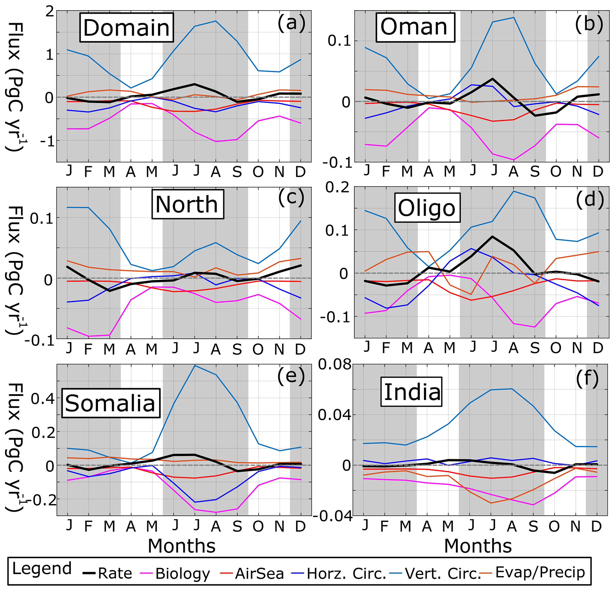
Figure 12Time series of DIC fluxes (Pg C yr−1) in the top 20 m for (a) the domain, (b) Oman, (c) north AS, (d) oligotrophic central AS, (e) Somalia, and (f) India. Dashed gray line shows x = 0 axis. Gray shading denotes summer and winter monsoons.
3.4 Near-surface DIC budgets and cycling
SST's effect on pCO2 reflects physical processes like surface heating and cooling, mixing, and advection. DIC, by contrast, reflects both physical and biological processes because in addition it is also impacted by photosynthesis, CaCO3 shell formation and dissolution, zooplankton respiration, detritus remineralization (bacterial respiration), and air–sea exchange. Budgets of DIC fluxes in the upper 20 m (Fig. 12; see Fig. S11 in the Supplement for a volume-specific DIC flux) show that two major processes dominate: vertical circulation (light blue lines) and net biological processes (magenta lines). In the entire domain and all subregions, and for all months, vertical circulation (advection and mixing) acts as a source of DIC, with the sum of all biological processes acting as a sink (NB the top 20 m does not constitute the entire euphotic zone, so respiration and remineralization at depth is not included). Maximum magnitudes of both vertical circulation and biological flux occur during the summer monsoon for all regions except for the north AS where they occur during the winter monsoon bloom (Fig. 12c). The maximum DIC flux in the domain due to vertical circulation is 1.76 Pg C yr−1, whereas biological flux peaks at −1.0 Pg C yr−1. Biological fluxes are nearly phase-matched with vertical circulation, though peaks in summer biological flux lag vertical circulation by a month (Fig. 12d, e, and f). Comparing the two flux terms, after normalizing biological flux by vertical circulation flux, the relative strength of biological processes vs. vertical sources of DIC becomes apparent. In the whole domain, biological flux ranges from −90 % to −34.5 % of vertical flux, similar to Rixen et al. (2005). As a result, biological fixation of carbon is generally weaker than physical vertical delivery of DIC.
Air–sea flux (red lines) is always negative due to the high pCO2 values, peaking during the summer monsoon. DIC flux due to atmospheric escape, while reaching its maximum magnitude of ∼ 0.32 Pg C yr−1 in June and July for the whole domain (Fig. 12a), only surpasses biological flux in May, when 0.23 Pg C yr−1 is released to the atmosphere compared to 0.15 Pg C yr−1 in biological processes. Evaporation and precipitation (brown lines) result in higher DIC for most of the year in the entire domain and upwelling regions (i.e., net evaporation, averaging 0.07 Pg C yr−1 in the domain) except India where it is negative (net precipitation, averaging −4.8 × 10⁻³ Pg C yr−1). The oligotrophic region's evaporation and precipitation flux (Fig. 12d) oscillates from being either positive or negative four times during the year, with magnitudes rivaling air–sea flux at times (5 × 10⁻² Pg C yr−1). Horizontal advection (dark blue lines) is negative on average for the whole domain (−0.2 Pg C yr−1), denoting net export (Fig. 12a). The same pattern occurs for all subregions except India with net horizontal import of surface DIC (Fig. 12f; 2.9 × 10⁻³ Pg C yr−1). The Omani upwelling region and the oligotrophic region experience positive peaks of horizontal import during the summer monsoon (27 and 56 Tg C yr−1 for Omani and oligotrophic regions, respectively), though for Somalia this period is the maximum DIC export, peaking at 220 Tg C yr−1 in July.
4.1 Model pCO2 vs. data
The pCO2 output from the model has a positive bias with respect to the in situ data, as is clear from Figs. 3 to 5. The question becomes whether the model bias precludes its use in acquiring a reasonable air–sea CO2 flux estimate. Regarding the direction of CO2 flux (positive outgassing or negative uptake), since most in situ ΔpCO2 data are already positive (Fig. 2), an additional positive bias will not impact flux direction, reaffirming the previous findings of Sarma et al. (1998) and subsequent work demonstrating that the AS is a source of CO2 to the atmosphere. A positive model bias in pCO2 has been noted in previous modeling studies. For instance, in the global data assimilation study of Valsala and Maksyutov (2010), they found an overall positive bias in the northern Indian Ocean, ∼ +5–15 µatm above TK09 (compared to our −3.1 to +48.4 µatm with respect to in situ data). Additionally, that study found a similar underestimate near the upwelling regions (summer negative bias in the model) of the AS and overestimate elsewhere (their Figs. 3 and 4). In Sreeush et al. (2019a), ROMS resulted in a systematic positive pCO2 bias, whereas the offline Ocean Transport Tracer Model (OTTM) produced negative bias in pCO2 in comparison to TK09.
The search for the model bias source is hindered by the lack of in situ data in the region. As already noted, GLODAP has 334 locations with DIC and TA in the top 50 m. The few available in situ data that do exist in the AS have a number of deficiencies for the purpose of validating model output. First, the data available are both old and concentrated around the years 1995 and 1997. While the JGOFS studies were quintessential in diagnosing the seasonal cycle of pCO2, they preclude being able to decipher the secular trend in surface pCO2 due to increasing atmospheric CO2 concentrations. In our analysis, we estimated a +2 µatm yr−1 trend, close to that of Tjiputra et al. (2014), though finding an interannual linear trend requires more data at regular intervals. Second, due to the nature of strong upwelling in the AS, previous cruise sampling also biases not only the summer months (≈70 % of data) but also places in the vicinity of the Omani coast (Fig. 3g). As a result, it is difficult to determine to what extent the data are representative of the entire AS. Consider that in the model, flux intensities are lower in the central, oligotrophic region (Fig. 6), but due to its surface area the total flux (28.6 Tg C yr−1) was close to that of Somalia (32.9 Tg C yr−1), an observation also made by Lendt et al. (2003). Determining to what extent the model over- or underestimates CO2 flux due to pCO2 bias would require more in situ sampling, which would need to be designed around solving the problems of areal coverage (outside of Oman and upwelling zones) and temporal coverage (off-summer months and recurrent over multiple years).
The distribution of model pCO2 is both similar to and different from previous data-based and modeling studies. Apart from the aforementioned bias leading to heightened absolute values (though Bates et al., 2006, have > 400 µatm for large parts of the AS), the relatively enhanced pCO2 values near Oman, along the west coast of India, and in the Gulf of Aden have already been observed (Sabine et al., 2000; Bates et al., 2006; Sarma et al., 2000; Körtzinger et al., 1997). These same studies, however, note a minimum of pCO2 outside of the summer monsoon near the southwest coast of India due to freshwater influx, which is not replicated well in the model. Additionally, elevated pCO2 near the Equator is not observed (Sabine et al., 2000; Bates et al., 2006), although it can appear in other models (Valsala and Murtugudde, 2015). The model's seasonal pCO2 minimum during the winter monsoon is also not reflective of results found elsewhere (Goyet et al., 1998a, b; Bates et al., 2006; though many studies highlight the north AS, where minimum model pCO2 occurs during the spring). Instead, these papers state pCO2 is minimal during the fall intermonsoon. Likewise, the large-scale spring maximum of pCO2 seen in the model is not found in these studies, except for in Louanchi et al. (1996), though this result is somewhat anomalous since that study showed a pCO2 minimum during the summer monsoon. Thus, while the model agrees with previous work insofar as the coastal regions impacted by upwelling show enhanced pCO2, mismatches do appear in the seasonal timing of maxima and minima, especially within certain subregions.
Despite the model's limitations, its advantages are also clear. Beyond the obvious increase in spatiotemporal coverage, capturing the monsoon's strong seasonal dynamics helps the model where other approaches fall short. This is especially illustrated in Fig. 5. Since upwelling regions are limited in geographic extent near the coast, capturing their high pCO2 values can be difficult for other approaches, such as TK09 with its coarse grid. Even the L15 product, with its finer grid, is unable to produce the higher pCO2 values seen during the summer. Judging from these comparisons, the trade-off appears to be that the model currently may produce less accurate pCO2 values outside of summer, but the explicit resolving of upwelling allows for enhanced pCO2 values during the summer monsoon, the peak of CO2 flux.
4.2 Spatial distribution of air–sea CO2 flux and pCO2
The model results both affirm the conclusions of previous studies in terms of CO2 flux direction and seasonality and yet find difference in magnitudes. As previously stated, the AS is an atmospheric CO2 source, with most flux occurring (56 %) during the summer monsoon (Fig. 6). In our results, however, there is no region during any of the seasons where CO2 uptake takes place. While somewhat expected, this is still in disagreement with some of the other pCO2 datasets previously considered, such as in Sarma (2003), in which negative ΔpCO2 values appear, such as during the winter monsoon near the south coast of India. The model's positive pCO2 bias may be to blame for this, making it so that no negative ΔpCO2 appears. Despite the positive pCO2 bias, a few other patterns are clear in comparison to other CO2 flux estimates. Sabine et al. (2000) and Sarma (2003) both find the maximum flux occurring during the summer monsoon centered around the upwelling regions, which is also quite visible in the model results (Fig. 6d). However, Bates et al. (2006) found that a secondary maximum of flux occurs during the winter monsoon, though due to the color scale in their Fig. 6 it is difficult to ascertain much beyond CO2 outgassing from the AS during all months of the year. Their secondary max in flux may be partly attributable to higher wintertime pCO2, as well.
The spatial decomposition of factors influencing pCO2 (Fig. 10) highlights how geographically DIC can be the strongest factor, with SST and TA taking secondary roles and SSS being a weak contributor. Since DIC and TA can co-vary with salinity, when they are not normalized, their distribution in the AS mirrors the north–south salinity gradient (see Figs. 2 and 3 in Bates et al., 2006). Once corrected for salinity, it is clear that the upwelling region of Oman still has elevated DIC, whereas the central, oligotrophic AS shows a DIC deficit. By contrast, the onshore–offshore gradient in TA is weaker. Differences between coastal and offshore normalized DIC and TA in the AS have been previously observed (Millero et al., 1998b; Lendt et al., 2003), but the stronger relative absence of DIC in the central AS and its role in affecting pCO2 has not been emphasized. A similar analysis in the California Current upwelling system (Turi et al., 2014) indicates near-compensation of DIC and temperature in opposing directions, nearly overlapping each other. In that scenario, DIC overpowers temperature at the coast, with TA and SSS being secondary. For the AS, while the upwelling regions of Oman and Somalia show temperature and DIC working against each other, they are not as well compensated for. Furthermore, the gradients of positive/negative pCO2 contributions from temperature and DIC do not overlap, leading to the curious scenario in which temperature and DIC both contribute positively to the pCO2 anomaly along the Indian coast. The positioning of these gradients and the surprising negative influence of DIC away from upwelling regions perhaps underscores how the AS is rather unique, where strong seasonal upwelling winds mingle with strong tropical heating and there is the influence of outflows from marginal seas (Prasad et al., 2001; l'Hégaret et al., 2015).
4.3 Seasonality of air–sea CO2 flux, pCO2, and DIC
4.3.1 Air–sea CO2 Flux
The fact that model CO2 flux for the entire domain peaks in summer despite a spring peak in pCO2 for the domain as a whole (along with the Somalian and oligotrophic regions) is the first sign that perhaps pCO2 is not the primary driver in determining flux timing. The Reynolds decomposition of CO2 flux terms (Fig. 8) clearly shows that a large proportion of the summer flux is due to the arrival of the strong southwest summer monsoon winds. The positive contributions due to pCO2 occur in the usual upwelling regions, though their contribution in magnitude is relatively muted and negative in the southern portion of the AS. Cross-terms, while non-zero, are inconsequential in determining the overall anomaly in summer flux intensity, as has been seen elsewhere (Doney et al., 2009b). Indeed, in a scenario in which the cross-term contribution is at its maximum amplitude, the Omani upwelling region during summer, the cross-term is not strong enough to sway the direction of the flux anomaly.
The summer flux signal is such that in nearly all the regions outside of summer, the anomaly is negative. Furthermore, the contribution of winds in particular is so strong that it is the largest factor all year except for the spring intermonsoon, when peak pCO2 is important relative to the effects of wind (or lack thereof) in the central oligotrophic AS, Somalia, and the averaged domain. This suggests that, on first order, winds are the most important factor in determining the seasonal air–sea flux cycle in the AS. We should keep in mind, however, that these results conflict with the analysis of Roobaert et al. (2019). In their global study of coastal waters, while seasonal CO2 flux variability in the AS is relatively high compared to other regions (their Fig. 6), the largest contributions come from ΔpCO2 and cross-terms (their Fig. 7), especially near the Horn of Africa. As a result, further work should be conducted to reduce uncertainty in sea surface pCO2 values to determine whether winds, ΔpCO2, or cross-terms are significant drivers of air–sea flux. Additionally, when considering the inconsistencies of models in estimating air–sea CO2 flux (Sarma et al., 2013), uncertainties from incomplete representation of winds and the various parameterizations of piston velocity must be considered in addition to pCO2, especially in light of recent work in the field (Ho et al., 2006; Wanninkhof, 2014; Roobaert et al., 2018).
Wind parameterizations notwithstanding, once winds are controlled in our metaanalysis (Fig. 9) it appears that on balance (1) gridded data-based pCO2 products will underestimate the upwelling zone maxima of pCO2 and CO2 flux during the summer, (2) the model overestimates pCO2 the rest of the year, eventually contributing to a possible overestimate of CO2 flux, and (3) this leaves reality somewhere in between. The only way to rectify these differences and arrive at a more accurate estimate will be to conduct sufficient in situ sampling of DIC, TA, and pCO2 in more regions than the upwelling zones, as well as preferably outside of the summer and over the course of multiple years. With the advent of ARGO floats with pH sensors, and the advancement of technology for other variables such as TA, the possibility emerges of using autonomous sampling platforms to expand beyond the limitations of shipboard measurements to fill the data gap in the AS carbon system.
4.3.2 The pCO2 seasonality
Decomposition of seasonal pCO2 anomalies within regions portrays a slightly different picture where temperature is the dominant force, with DIC countervailing in the upwelling regions. Not only is this seasonal cycle more akin to that seen in the California Current (Turi et al., 2014), the dueling role of these two forces is also reflected in a similar analysis by Sreeush et al. (2019a) for pH instead of pCO2 in the AS. Interestingly, in that study both ROMS and OTTM were compared side-by-side, and in OTTM, TA played a larger role than in ROMS. Similarly, in Valsala and Maksyutov (2013), TA played an important role in regulating interannual pCO2 variability in the AS. A preliminary TA budget of the model (Fig. S12 in the Supplement) shows that while vertical circulation and biological processes dominate the seasonal cycle of near-surface DIC, TA has multiple forces influencing its time evolution. However, the magnitude of the fluxes are ∼ those of DIC, indicating that TA is less seasonally variable than DIC (reflected also in Fig. 11). These results, from another model, as well as the low variability in this model's TA, raise the possibility that TA's importance is underestimated in the current study.
Zooming out from the upwelling regions and looking at the whole AS, the dominance of temperature on the seasonal pCO2 cycle is clear. In the domain average, temperature effects nearly overlap with the overall pCO2 anomaly. This result brings back into focus the seasonal timing of pCO2 minima and maxima in the model vis à vis previous work. In the earlier studies, which either use data directly or build statistical models from those data, there is no spring intermonsoon pCO2 maximum driven by heating. Indeed, Sabine et al. (2000) noted that pCO2 in the spring was much lower than would be expected given the SST but attributed this to drawdown due to biological production. The model, however, indicates that this is precisely the season when biological production is at its lowest. The presence of these springtime maxima can be seen in other models, as is visible in the results of Valsala and Maksyutov (2010) and a synthesis by Sarma et al. (2013). Since the model indicates temperature is producing the maxima, it reduces the concern that erroneous DIC or TA values in the model are driving this signal. The model SST matches well with the in situ data (Figs. S8 and S9), and the forcing datasets for SST and heat flux correspond to data that predate or include the pCO2 sampling period (i.e., before 2000), so a climate change bias is unlikely. What might be more likely, then, is a sampling bias towards summertime Oman, one of the few areas in the AS with a summertime instead of springtime pCO2 max. Such a bias could possibly obscure what is happening in the rest of the AS. Regardless, the discrepancy between models and observations during the spring period can be added as yet another reason to conduct more in situ sampling to either confirm or disavow whether the model results are spurious.
4.3.3 DIC seasonality
The potential for biological control in setting pCO2 has been found in Sri Lanka near the AS (Chakraborty et al., 2018). In this study, it was found that the source water in Sri Lanka was sufficiently low in DIC relative to inorganic nutrients that upwelling actually reduced surface pCO2. In a similar vein, Takahashi et al. (2002) found, using a metric comparing temperature and “biological” effects (i.e., everything else), that the AS's pCO2 is reduced more by biological production than temperature effects. Conducting this analysis on the model output (Fig. S13 in the Supplement), it appears that “biological” control appears dominant over the upwelling areas (Omani coast, coast of Somalia, India) and near the Equator east of 60∘ E, but for the majority of the AS temperature dominates. This cursory analysis aside, as is evident in the results of Chakraborty et al. (2018), the more useful comparison is in determining whether biological production is sufficient to outweigh DIC enhancement from subsurface water.
In summary, the results in Fig. 12 indicate that for the entire AS, DIC enhancement by vertical circulation (both advection and mixing) brings more DIC into the near-surface than is removed by net biological processes, and so no biologically induced decrease in pCO2 occurs in the final pCO2 signal. The timing of biological drawdown, occurring at the same time or lagging vertical circulation, is consistent with the general phenology of blooms and similar to previous findings (Louanchi et al., 1996; Rixen et al., 2006; Sharada et al., 2008). The result that biological cycling of carbon is much larger than the air–sea flux of CO2 also corroborates the results of Lendt et al. (2003), who found net community production to be ∼ 3.6 times larger than CO2 emission. The relatively low impact of horizontal advection is an interesting detail to consider; in other upwelling systems, significant proportions of water and biological production are advected offshore (Nagai et al., 2015). Lendt et al. (2003) suggest upwelled nitrate is assimilated and does not arrive in the central AS, while Resplandy et al. (2011) show that a large fraction of total nutrients in the central AS come from the upwelling zones. Thus, although water may be advected offshore, the relevant timescale for DIC cycling processes (i.e., air–sea emission, biological uptake) may be short enough so that horizontal export of enhanced DIC (keep in mind the onshore–offshore normalized DIC gradient) from the upwelling regions does not significantly contribute to the central AS or other regions.
In this study, we used a regional circulation model coupled with a biogeochemical model to investigate the annual magnitude, seasonal cycle, and drivers of air–sea CO2 flux in the AS, primarily winds and ΔpCO2. This effort was made to complement previous flux estimates, for which limited data or insufficient model resolutions have produced contrasting results. Consistent with previous work, we find that the AS is a source of CO2 to the atmosphere for the entire year, with the bulk occurring during the summer monsoon. Our estimate of flux, ∼ 160 Tg C yr−1, with concentrated flux densities up to 6 in the upwelling regions, is larger than most previous reports but not inconsistent with the range of other findings (Sarma, 2003; Naqvi et al., 2005; Sarma et al., 2013) . Since the AS lacks carbon data, here we subjected the model to validation with raw data instead of smoothed climatologies. The model is shown to have a positive bias in pCO2, attributed to TA and DIC, with TA bias being stronger. Despite this, pCO2 variability compares favorably to alternative products in the region. The bias results in strongly positive ΔpCO2 throughout the domain year-round. While positive ΔpCO2 values have been observed before in the AS, we likely overestimate CO2 flux outside of the summer monsoon.
The majority of flux occurs during the summer as opposed to a modeled spring pCO2 maximum due to the influence of winds. A Reynolds decomposition of both pCO2 and wind variability shows that the intense winds of the summer monsoon contribute 90 % of that season's flux anomaly. In fact, winds play a more important role than the increase in pCO2 in the upwelling regions. Even though winds represent such a major variable in determining AS CO2 flux timing, the variability in total flux due to different pCO2 products leads to a 2× range in magnitude. These results suggest that in addition to the expected increase in surface ocean pCO2 due to anthropogenic climate change, possible changes in the timing, location, and magnitude of monsoon winds (Lachkar et al., 2018; Praveen et al., 2020) will have downstream impacts on seasonal air–sea flux.
An important result of this modeling study is that temperature drives a springtime maximum of pCO2 in the AS. This maximum has been observed in lower-resolution models but is not found in the in situ data. Due to the fact that temperature is not sensitive to biological processes like DIC and TA, this discrepancy suggests that more sampling is necessary to determine whether it is an artifact of spotty sampling or an inherent problem in models unrelated to resolving coastal upwelling. Additionally, we find that spatial gradients of DIC and temperature do not overlap as they do elsewhere in the ocean. Instead, temperature follows a southwest–northeast monsoon wind pattern, whereas DIC is enhanced nearest to the coasts. The resulting apparent deficit of normalized DIC in the central, oligotrophic AS has not been emphasized previously. Finally, we find that despite the intense biological activity in the AS, primary production by phytoplankton is insufficient to counter the increased carbon supply provided by vertical circulation during bloom periods.
Models can be used to expand spatiotemporal coverage when data are scarce. However, models' limitations often manifest when there are no new data to test their fidelity. Limitations in the spatiotemporal coverage of existing datasets stem from biases in sampling during the summer monsoon, sampling close to the Omani upwelling region, and sampling limited in scope to the years of JGOFS expeditions of the 1990s. In order to fully characterize the pCO2 cycle outside of summer in the rest of the AS, as well as to determine the secular trend of surface pCO2 due to anthropogenic carbon additions to the atmosphere, more in situ data of the carbon system (e.g., DIC, TA, pCO2), from shipboard measurements or autonomous sampling platforms, are sorely needed. Finally since ΔpCO2 is generally positive in the AS, the direction of air–sea CO2 exchange examined here is robust to model error, whereas other important indicators such as pH and aragonite saturation, Ωa, which at important thresholds of low values have deleterious impacts for various biological taxa (Doney et al., 2009a; Bednaršek et al., 2019, 2021) will be less so. These data are thus critical for resolving the possible responses of the carbon system in the AS to ongoing climate change, whether from changes in timing or magnitude of monsoon wind forcing, the impact of increased surface heating on stratification and vertical circulation, or changing levels of primary and fisheries productivity with altered carbonate solubility. Without this baseline information, it will be difficult to predict what the future has in store for the AS carbon system.
ROMS-AGRIF is provided by https://www.croco-ocean.org (last access: 1 February 2022).
Model output used in this study can be accessed and cited from the following: https://doi.org/10.5281/zenodo.5937512 (de Verneil, 2022). The Surface Ocean CO2 Atlas (SOCAT; Bakker et al., 2016) can be downloaded from https://www.socat.info/index.php/version-2019/ (last access: 1 February 2022). The Lamont–Doherty Earth Observatory pCO2 database can be downloaded from https://www.ncei.noaa.gov/access/ocean-carbon-data-system/oceans/LDEO_Underway_Database/ (last access: 1 February 2022). The Simple Ocean Data Assimilation (SODA) reanalysis data can be downloaded from http://apdrc.soest.hawaii.edu/datadoc/soda_2.2.4.php (last access: 1 February 2022). The World Ocean Atlas 2009 can be downloaded from https://www.ncei.noaa.gov/data/oceans/woa/WOA09/DATA/ (last access: 1 February 2022). The Comprehensive Ocean-Atmosphere Data Set (COADS) can be downloaded from http://iridl.ldeo.columbia.edu/SOURCES/.DASILVA/.SMD94/.halfbyhalf/.climatology/ (last access: 1 February 2022). The Scatterometer Climatology of Ocean Winds (SCOW) can be downloaded from https://chapman.ceoas.oregonstate.edu/scow/index.html (last access: 1 February 2022). AVHRR SST data can be downloaded from https://www.ncei.noaa.gov/data/oceans/pathfinder/Version5.0_Climatologies/1982_2008/Monthly/ (last access: 1 February 2022). NPP data can be downloaded from https://sites.science.oregonstate.edu/ocean.productivity/custom.php (last access: 1 February 2022).
The supplement related to this article is available online at: https://doi.org/10.5194/bg-19-907-2022-supplement.
AdV, ZL, and ML conceived the study, AdV and ZL ran the model, AdV, ZL, SS, and ML conducted analysis, AdV generated figures and text, and ZL, SS, and ML revised figures and text.
The contact author has declared that neither they nor their co-authors have any competing interests.
Publisher's note: Copernicus Publications remains neutral with regard to jurisdictional claims in published maps and institutional affiliations.
Support for this research comes from the Center for Prototype Climate Modeling (CPCM), the New York University Abu Dhabi (NYUAD) Research Institute. Computations were conducted at the High Performance Cluster (HPC) at NYUAD, Dalma. We deeply thank both Benoit Merchand and Muataz Al Barwani for their technical support. We are also grateful for the work of two anonymous reviewers and associate editor Peter Landschützer, who greatly improved the manuscript.
This research has been supported by Tamkeen under the NYU Abu Dhabi Research Institute (grant nos. G110 and CG009).
This paper was edited by Peter Landschützer and reviewed by two anonymous referees.
Acharya, S. S. and Panigrahi, M. K.: Eastward shift and maintenance of Arabian Sea oxygen minimum zone: Understanding the paradox, Deep-Sea Res. Pt. I, 115, 240–252, 2016. a
Bakker, D. C. E., Pfeil, B., Landa, C. S., Metzl, N., O'Brien, K. M., Olsen, A., Smith, K., Cosca, C., Harasawa, S., Jones, S. D., Nakaoka, S., Nojiri, Y., Schuster, U., Steinhoff, T., Sweeney, C., Takahashi, T., Tilbrook, B., Wada, C., Wanninkhof, R., Alin, S. R., Balestrini, C. F., Barbero, L., Bates, N. R., Bianchi, A. A., Bonou, F., Boutin, J., Bozec, Y., Burger, E. F., Cai, W.-J., Castle, R. D., Chen, L., Chierici, M., Currie, K., Evans, W., Featherstone, C., Feely, R. A., Fransson, A., Goyet, C., Greenwood, N., Gregor, L., Hankin, S., Hardman-Mountford, N. J., Harlay, J., Hauck, J., Hoppema, M., Humphreys, M. P., Hunt, C. W., Huss, B., Ibánhez, J. S. P., Johannessen, T., Keeling, R., Kitidis, V., Körtzinger, A., Kozyr, A., Krasakopoulou, E., Kuwata, A., Landschützer, P., Lauvset, S. K., Lefèvre, N., Lo Monaco, C., Manke, A., Mathis, J. T., Merlivat, L., Millero, F. J., Monteiro, P. M. S., Munro, D. R., Murata, A., Newberger, T., Omar, A. M., Ono, T., Paterson, K., Pearce, D., Pierrot, D., Robbins, L. L., Saito, S., Salisbury, J., Schlitzer, R., Schneider, B., Schweitzer, R., Sieger, R., Skjelvan, I., Sullivan, K. F., Sutherland, S. C., Sutton, A. J., Tadokoro, K., Telszewski, M., Tuma, M., van Heuven, S. M. A. C., Vandemark, D., Ward, B., Watson, A. J., and Xu, S.: A multi-decade record of high-quality fCO2 data in version 3 of the Surface Ocean CO2 Atlas (SOCAT), Earth Syst. Sci. Data, 8, 383–413, https://doi.org/10.5194/essd-8-383-2016, 2016. a, b
Bates, N. R., Pequignet, A. C., and Sabine, C. L.: Ocean carbon cycling in the Indian Ocean: 1. Spatiotemporal variability of inorganic carbon and air–sea CO2 gas exchange, Global Biogeochem. Cy., 20, GB3020, https://doi.org/10.1029/2005GB002491, 2006. a, b, c, d, e, f, g
Bednaršek, N., Feely, R. A., Howes, E. L., Hunt, B. P. V., Kessouri, F., León, P., Lischka, S., Maas, A. E., McLaughlin, K., Nezlin, N. P., Sutula, M., and Weisberg, S. B.: Systematic Review and Meta-Analysis Toward Synthesis of Thresholds of Ocean Acidification Impacts on Calcifying Pteropods and Interactions With Warming, Frontiers in Marine Science, 6, 227, https://doi.org/10.3389/fmars.2019.00227, 2019. a
Bednaršek, N., Calosi, P., Feely, R. A., Ambrose, R., Byrne, M., Chan, K. Y. K., Dupont, S., Padilla-Gamiño, J. L., Spicer, J. I., Kessouri, F., Roethler, M., Sutula, M., and Weisberg, S. B.: Synthesis of Thresholds of Ocean Acidification Impacts on Echinoderms, Frontiers in Marine Science, 8, 261, https://doi.org/10.3389/fmars.2021.602601, 2021. a
Behrenfeld, M. J. and Falkowski, P. G.: Photosynthetic rates derived from satellite-based chlorophyll concentration, Limnol. Oceanogr., 42, 1–20, https://doi.org/10.4319/lo.1997.42.1.0001, 1997. a
Carton, J. A. and Giese, B. S.: A reanalysis of ocean climate using Simple Ocean Data Assimilation (SODA), Mon. Weather Rev., 136, 2999–3017, 2008. a
Casey, K. S. and Cornillon, P.: A comparison of satellite and in situ–based sea surface temperature climatologies, J. Climate, 12, 1848–1863, 1999. a
Chakraborty, K., Valsala, V., Gupta, G., and Sarma, V.: Dominant biological control over upwelling on pCO2 in sea east of Sri Lanka, J. Geophys. Res.-Biogeo., 123, 3250–3261, 2018. a, b, c
Ciais, P., Sabine, C., Bala, G., Bopp, L., Brovkin, V., Canadell, J., Chhabra, A., DeFries, R., Galloway, J., Heimann, M., Jones, C., Le Quéré, C., Myneni, R. B., Piao, S., and Thornton, P.: Carbon and Other Biogeochemical Cycles, in: Climate Change 2013: The Physical Science Basis. Contribution of Working Group I to the Fifth Assessment Report of the Intergovernmental Panel on Climate Change, edited by: Stocker, T. F., Qin, D., Plattner, G. K., Tignor, M., Allen, S.K., Boschung, J., Nauels, A., Xia, Y., Bex, V., Midgley, P. M., Cambridge University Press, Cambridge, United Kingdom and New York, NY, USA, 2013. a
Curry, W., Ostermann, D., Guptha, M., and Ittekkot, V.: Foraminiferal production and monsoonal upwelling in the Arabian Sea: evidence from sediment traps, Geological Society, London, Special Publications, 64, 93–106, 1992. a
da Silva, A. M., Young, C. C., and Levitus, S.: Atlas of surface marine data 1994, Vol. 4: Anomalies of fresh water fluxes, NOAA Atlas, NESDIS, U.S. Department of Commerce, NOAA, NESDIS, 9, 1994. a
de Verneil, A.: Evaluating the Arabian Sea as a regional source of atmospheric CO2: seasonal variability and drivers, Zenodo [Data set], https://doi.org/10.5281/zenodo.5937512, 2022. a
Dickson, A. and Millero, F. J.: A comparison of the equilibrium constants for the dissociation of carbonic acid in seawater media, Deep-Sea Res. Pt. I, 34, 1733–1743, 1987. a
Doney, S. C., Fabry, V. J., Feely, R. A., and Kleypas, J. A.: Ocean Acidification: The Other CO2 Problem, Annu. Rev. Mar. Sci., 1, 169–192, https://doi.org/10.1146/annurev.marine.010908.163834, pMID: 21141034, 2009a. a
Doney, S. C., Lima, I., Feely, R. A., Glover, D. M., Lindsay, K., Mahowald, N., Moore, J. K., and Wanninkhof, R.: Mechanisms governing interannual variability in upper-ocean inorganic carbon system and air–sea CO2 fluxes: Physical climate and atmospheric dust, Deep-Sea Res. Pt. II, 56, 640–655, 2009b. a, b
Friedlingstein, P., O'Sullivan, M., Jones, M. W., Andrew, R. M., Hauck, J., Olsen, A., Peters, G. P., Peters, W., Pongratz, J., Sitch, S., Le Quéré, C., Canadell, J. G., Ciais, P., Jackson, R. B., Alin, S., Aragão, L. E. O. C., Arneth, A., Arora, V., Bates, N. R., Becker, M., Benoit-Cattin, A., Bittig, H. C., Bopp, L., Bultan, S., Chandra, N., Chevallier, F., Chini, L. P., Evans, W., Florentie, L., Forster, P. M., Gasser, T., Gehlen, M., Gilfillan, D., Gkritzalis, T., Gregor, L., Gruber, N., Harris, I., Hartung, K., Haverd, V., Houghton, R. A., Ilyina, T., Jain, A. K., Joetzjer, E., Kadono, K., Kato, E., Kitidis, V., Korsbakken, J. I., Landschützer, P., Lefèvre, N., Lenton, A., Lienert, S., Liu, Z., Lombardozzi, D., Marland, G., Metzl, N., Munro, D. R., Nabel, J. E. M. S., Nakaoka, S.-I., Niwa, Y., O'Brien, K., Ono, T., Palmer, P. I., Pierrot, D., Poulter, B., Resplandy, L., Robertson, E., Rödenbeck, C., Schwinger, J., Séférian, R., Skjelvan, I., Smith, A. J. P., Sutton, A. J., Tanhua, T., Tans, P. P., Tian, H., Tilbrook, B., van der Werf, G., Vuichard, N., Walker, A. P., Wanninkhof, R., Watson, A. J., Willis, D., Wiltshire, A. J., Yuan, W., Yue, X., and Zaehle, S.: Global Carbon Budget 2020, Earth Syst. Sci. Data, 12, 3269–3340, https://doi.org/10.5194/essd-12-3269-2020, 2020. a
Goyet, C., Metzl, N., Millero, F., Eischeid, G., O'sullivan, D., and Poisson, A.: Temporal variation of the sea surface CO2/carbonate properties in the Arabian Sea, Mar. Chem., 63, 69–79, 1998a. a
Goyet, C., Millero, F. J., O'Sullivan, D., Eischeid, G., McCue, S., and Bellerby, R.: Temporal variations of pCO2 in surface seawater of the Arabian Sea in 1995, Deep-Sea Res. Pt. I, 45, 609–623, 1998b. a, b, c
Gruber, N., Frenzel, H., Doney, S. C., Marchesiello, P., McWilliams, J. C., Moisan, J. R., Oram, J. J., Plattner, G.-K., and Stolzenbach, K. D.: Eddy-resolving simulation of plankton ecosystem dynamics in the California Current System, Deep-Sea Res. Pt. I, 53, 1483–1516, 2006. a
Gruber, N., Lachkar, Z., Frenzel, H., Marchesiello, P., Münnich, M., McWilliams, J. C., Nagai, T., and Plattner, G.-K.: Eddy-induced reduction of biological production in eastern boundary upwelling systems, Nat. Geosci., 4, 787–792, 2011. a
Gruber, N., Hauri, C., Lachkar, Z., Loher, D., Frölicher, T. L., and Plattner, G.-K.: Rapid progression of ocean acidification in the California Current System, Science, 337, 220–223, 2012. a
Hauri, C., Gruber, N., Vogt, M., Doney, S. C., Feely, R. A., Lachkar, Z., Leinweber, A., McDonnell, A. M. P., Munnich, M., and Plattner, G.-K.: Spatiotemporal variability and long-term trends of ocean acidification in the California Current System, Biogeosciences, 10, 193–216, https://doi.org/10.5194/bg-10-193-2013, 2013. a
Ho, D. T., Law, C. S., Smith, M. J., Schlosser, P., Harvey, M., and Hill, P.: Measurements of air-sea gas exchange at high wind speeds in the Southern Ocean: Implications for global parameterizations, Geophys. Res. Lett., 33, L16611, https://doi.org/10.1029/2006GL026817, 2006. a
Hood, R. R., Urban, E. R., McPhaden, M. J., Su, D., and Raes, E.: The 2nd International Indian Ocean Expedition (IIOE-2): Motivating New Exploration in a Poorly Understood Basin, Limnology and Oceanography Bulletin, 25, 117–124, 2016. a
Keeling, C. D.: Carbon dioxide in surface ocean waters: 4. Global distribution, J. Geophys. Res., 73, 4543–4553, https://doi.org/10.1029/JB073i014p04543, 1968. a
Keeling, C. D., Brix, H., and Gruber, N.: Seasonal and long-term dynamics of the upper ocean carbon cycle at Station ALOHA near Hawaii, Global Biogeochem. Cy., 18, GB4006, https://doi.org/10.1029/2004GB002227, 2004. a
Khatiwala, S., Primeau, F., and Hall, T.: Reconstruction of the history of anthropogenic CO2 concentrations in the ocean, Nature, 462, 346–349, 2009. a
Körtzinger, A., Duinker, J. C., and Mintrop, L.: Strong CO2 emissions from the Arabian Sea during south-west monsoon, Geophys. Res. Lett., 24, 1763–1766, 1997. a
Kumar, S. P., Ramaiah, N., Gauns, M., Sarma, V., Muraleedharan, P., Raghukumar, S., Kumar, M. D., and Madhupratap, M.: Physical forcing of biological productivity in the Northern Arabian Sea during the Northeast Monsoon, Deep-Sea Res. Pt. II, 48, 1115–1126, 2001. a, b
Lachkar, Z. and Gruber, N.: Response of biological production and air–sea CO2 fluxes to upwelling intensification in the California and Canary Current Systems, J. Marine Syst., 109, 149–160, 2013. a
Lachkar, Z., Smith, S., Lévy, M., and Pauluis, O.: Eddies reduce denitrification and compress habitats in the Arabian Sea, Geophys. Res. Lett., 43, 9148–9156, 2016. a, b, c
Lachkar, Z., Lévy, M., and Smith, S.: Intensification and deepening of the Arabian Sea oxygen minimum zone in response to increase in Indian monsoon wind intensity, Biogeosciences, 15, 159–186, https://doi.org/10.5194/bg-15-159-2018, 2018. a
Landschützer, P., Gruber, N., Haumann, F. A., Rödenbeck, C., Bakker, D. C., Van Heuven, S., Hoppema, M., Metzl, N., Sweeney, C., Takahashi, T., Tilbrook, B., and Wanninkhof, R.: The reinvigoration of the Southern Ocean carbon sink, Science, 349, 1221–1224, 2015. a, b
Large, W. G., McWilliams, J. C., and Doney, S. C.: Oceanic vertical mixing: A review and a model with a nonlocal boundary layer parameterization, Rev. Geophys., 32, 363–403, 1994. a
Lee, K., Tong, L. T., Millero, F. J., Sabine, C. L., Dickson, A. G., Goyet, C., Park, G.-H., Wanninkhof, R., Feely, R. A., and Key, R. M.: Global relationships of total alkalinity with salinity and temperature in surface waters of the world's oceans, Geophys. Res. Lett., 33, L19605, https://doi.org/10.1029/2006GL027207, 2006. a
Lendt, R., Thomas, H., Hupe, A., and Ittekkot, V.: Response of the near-surface carbonate system of the northwestern Arabian Sea to the southwest monsoon and related biological forcing, J. Geophys. Res.-Oceans, 108, 3222, https://doi.org/10.1029/2000JC000771, 2003. a, b, c, d
Lévy, M., Shankar, D., André, J.-M., Shenoi, S., Durand, F., and de Boyer Montégut, C.: Basin-wide seasonal evolution of the Indian Ocean's phytoplankton blooms, J. Geophys. Res.-Oceans, 112, C12014, https://doi.org/10.1029/2007JC004090, 2007. a
L'Hégaret, P., Duarte, R., Carton, X., Vic, C., Ciani, D., Baraille, R., and Corréard, S.: Mesoscale variability in the Arabian Sea from HYCOM model results and observations: impact on the Persian Gulf Water path, Ocean Sci., 11, 667–693, https://doi.org/10.5194/os-11-667-2015, 2015. a
Louanchi, F., Metzl, N., and Poisson, A.: Modelling the monthly sea surface fCO2 fields in the Indian Ocean, Mar. Chem., 55, 265–279, 1996. a, b
Lovenduski, N. S., Gruber, N., Doney, S. C., and Lima, I. D.: Enhanced CO2 outgassing in the Southern Ocean from a positive phase of the Southern Annular Mode, Global Biogeochem. Cy., 21, GB2026, https://doi.org/10.1029/2006GB002900, 2007. a, b
Mahadevan, A., Lévy, M., and Mémery, L.: Mesoscale variability of sea surface pCO2: What does it respond to?, Global Biogeochem. Cy., 18, GB1017, https://doi.org/10.1029/2003GB002102, 2004. a
Mahadevan, A., Tagliabue, A., Bopp, L., Lenton, A., Mémery, L., and Lévy, M.: Impact of episodic vertical fluxes on sea surface pCO2, Philos. T. R. Soc. A, 369, 2009–2025, https://doi.org/10.1098/rsta.2010.0340, 2011. a
Marchesiello, P., Debreu, L., and Couvelard, X.: Spurious diapycnal mixing in terrain-following coordinate models: The problem and a solution, Ocean Model., 26, 156–169, 2009. a
Mehrbach, C., Culberson, C., Hawley, J., and Pytkowicx, R.: Measurement of the apparent dissociation constants of carbonic acid in seawater at atmospheric pressure 1, Limnol. Oceanogr., 18, 897–907, 1973. a
Millero, F. J.: Thermodynamics of the carbon dioxide system in the oceans, Geochim. Cosmochim. Acta, 59, 661–677, 1995. a
Millero, F. J., Degler, E. A., O'Sullivan, D. W., Goyet, C., and Eischeid, G.: The carbon dioxide system in the Arabian Sea, Deep-Sea Res. Pt. II, 45, 2225–2252, 1998a. a
Millero, F. J., Lee, K., and Roche, M.: Distribution of alkalinity in the surface waters of the major oceans, Mar. Chem., 60, 111–130, https://doi.org/10.1016/S0304-4203(97)00084-4, 1998b. a
Morrison, J. M., Codispoti, L., Smith, S. L., Wishner, K., Flagg, C., Gardner, W. D., Gaurin, S., Naqvi, S., Manghnani, V., Prosperie, L., Prosperie, L., and Gundersen, J. S.: The oxygen minimum zone in the Arabian Sea during 1995, Deep-Sea Res. Pt. II, 46, 1903–1931, 1999. a
Nagai, T., Gruber, N., Frenzel, H., Lachkar, Z., McWilliams, J. C., and Plattner, G.-K.: Dominant role of eddies and filaments in the offshore transport of carbon and nutrients in the California Current System, J. Geophys. Res.-Oceans, 120, 5318–5341, 2015. a
Naqvi, S. W. A., Gupta, R. S., and Kumar, M. D.: Carbon dioxide and nitrous oxide in the Arabian Sea, Geophysical Monograph Series, American Geophysical Union, Washington, DC, 75, 85–92, https://doi.org/10.1029/GM075p0085, 1993. a
Naqvi, S. W. A., Bange, H. W., Gibb, S. W., Goyet, C., Hatton, A. D., and Upstill-Goddard, R. C.: Biogeochemical ocean–atmosphere transfers in the Arabian Sea, Prog. Oceanogr., 65, 116–144, 2005. a, b, c
Olsen, A., Lange, N., Key, R. M., Tanhua, T., Álvarez, M., Becker, S., Bittig, H. C., Carter, B. R., Cotrim da Cunha, L., Feely, R. A., van Heuven, S., Hoppema, M., Ishii, M., Jeansson, E., Jones, S. D., Jutterström, S., Karlsen, M. K., Kozyr, A., Lauvset, S. K., Lo Monaco, C., Murata, A., Pérez, F. F., Pfeil, B., Schirnick, C., Steinfeldt, R., Suzuki, T., Telszewski, M., Tilbrook, B., Velo, A., and Wanninkhof, R.: GLODAPv2.2019 – an update of GLODAPv2, Earth Syst. Sci. Data, 11, 1437–1461, https://doi.org/10.5194/essd-11-1437-2019, 2019. a, b
Orr, J. C. and Epitalon, J.-M.: Improved routines to model the ocean carbonate system: mocsy 2.0, Geosci. Model Dev., 8, 485–499, https://doi.org/10.5194/gmd-8-485-2015, 2015. a
Orr, J. C., Epitalon, J.-M., Dickson, A. G., and Gattuso, J.-P.: Routine uncertainty propagation for the marine carbon dioxide system, Mar. Chem., 207, 84–107, 2018. a
Paulmier, A., Ruiz-Pino, D., and Garçon, V.: CO2 maximum in the oxygen minimum zone (OMZ), Biogeosciences, 8, 239–252, https://doi.org/10.5194/bg-8-239-2011, 2011. a
Pfeil, B., Olsen, A., Bakker, D. C. E., Hankin, S., Koyuk, H., Kozyr, A., Malczyk, J., Manke, A., Metzl, N., Sabine, C. L., Akl, J., Alin, S. R., Bates, N., Bellerby, R. G. J., Borges, A., Boutin, J., Brown, P. J., Cai, W.-J., Chavez, F. P., Chen, A., Cosca, C., Fassbender, A. J., Feely, R. A., González-Dávila, M., Goyet, C., Hales, B., Hardman-Mountford, N., Heinze, C., Hood, M., Hoppema, M., Hunt, C. W., Hydes, D., Ishii, M., Johannessen, T., Jones, S. D., Key, R. M., Körtzinger, A., Landschützer, P., Lauvset, S. K., Lefèvre, N., Lenton, A., Lourantou, A., Merlivat, L., Midorikawa, T., Mintrop, L., Miyazaki, C., Murata, A., Nakadate, A., Nakano, Y., Nakaoka, S., Nojiri, Y., Omar, A. M., Padin, X. A., Park, G.-H., Paterson, K., Perez, F. F., Pierrot, D., Poisson, A., Ríos, A. F., Santana-Casiano, J. M., Salisbury, J., Sarma, V. V. S. S., Schlitzer, R., Schneider, B., Schuster, U., Sieger, R., Skjelvan, I., Steinhoff, T., Suzuki, T., Takahashi, T., Tedesco, K., Telszewski, M., Thomas, H., Tilbrook, B., Tjiputra, J., Vandemark, D., Veness, T., Wanninkhof, R., Watson, A. J., Weiss, R., Wong, C. S., and Yoshikawa-Inoue, H.: A uniform, quality controlled Surface Ocean CO2 Atlas (SOCAT), Earth Syst. Sci. Data, 5, 125–143, https://doi.org/10.5194/essd-5-125-2013, 2013. a
Prasad, T., Ikeda, M., and Kumar, S. P.: Seasonal spreading of the Persian Gulf Water mass in the Arabian Sea, J. Geophys. Res.-Oceans, 106, 17059–17071, 2001. a
Praveen, V., Valsala, V., Ajayamohan, R., and Balasubramanian, S.: Oceanic Mixing over the Northern Arabian Sea in a Warming Scenario: Tug of War between Wind and Buoyancy Forces, J. Phys. Oceanogr., 50, 945–964, 2020. a
Resplandy, L., Lévy, M., Madec, G., Pous, S., Aumont, O., and Kumar, D.: Contribution of mesoscale processes to nutrient budgets in the Arabian Sea, J. Geophys. Res.-Oceans, 116, C11, https://doi.org/10.1029/2011JC007006, 2011. a
Resplandy, L., Lévy, M., and McGillicuddy Jr., D. J.: Effects of Eddy-Driven Subduction on Ocean Biological Carbon Pump, Global Biogeochem. Cy., 33, 1071–1084, https://doi.org/10.1029/2018GB006125, 2019. a
Risien, C. M. and Chelton, D. B.: A global climatology of surface wind and wind stress fields from eight years of QuikSCAT scatterometer data, J. Phys. Oceanogr., 38, 2379–2413, 2008. a
Rixen, T., Guptha, M., and Ittekkot, V.: Deep ocean fluxes and their link to surface ocean processes and the biological pump, Prog. Oceanogr., 65, 240–259, 2005. a
Rixen, T., Goyet, C., and Ittekkot, V.: Diatoms and their influence on the biologically mediated uptake of atmospheric CO2 in the Arabian Sea upwelling system, Biogeosciences, 3, 1–13, https://doi.org/10.5194/bg-3-1-2006, 2006. a
Roobaert, A., Laruelle, G. G., Landschützer, P., and Regnier, P.: Uncertainty in the global oceanic CO2 uptake induced by wind forcing: quantification and spatial analysis, Biogeosciences, 15, 1701–1720, https://doi.org/10.5194/bg-15-1701-2018, 2018. a
Roobaert, A., Laruelle, G. G., Landschützer, P., Gruber, N., Chou, L., and Regnier, P.: The spatiotemporal dynamics of the sources and sinks of CO2 in the global coastal ocean, Global Biogeochem. Cy., 33, 1693–1714, 2019. a
Sabine, C., Wanninkhof, R., Key, R., Goyet, C., and Millero, F. J.: Seasonal CO2 fluxes in the tropical and subtropical Indian Ocean, Mar. Chem., 72, 33–53, 2000. a, b, c, d, e
Sarma, V.: Monthly variability in surface pCO2 and net air–sea CO2 flux in the Arabian Sea, J. Geophys. Res.-Oceans, 108, 3255, https://doi.org/10.1029/2001JC001062, 2003. a, b, c, d, e, f, g, h, i, j, k, l, m, n
Sarma, V., Kumar, M. D., and George, M.: The central and eastern Arabian Sea as a perennial source of atmospheric carbon dioxide, Tellus B, 50, 179–184, 1998. a, b, c
Sarma, V., Swathi, P., Kumar, M. D., Prasannakumar, S., Bhattathiri, P., Madhupratap, M., Ramaswamy, V., Sarin, M., Gauns, M., Ramaiah, N., Sardessai, S., and de Sousa, S. N.: Carbon budget in the eastern and central Arabian Sea: An Indian JGOFS synthesis, Global Biogeochem. Cy., 17, 1102,https://doi.org/10.1029/2002GB001978, 2003. a
Sarma, V. V. S. S., Dileep, K. M., Gauns, M., and Madhupratap, M.: Seasonal controls on surface pCO2 in the central and eastern Arabian Sea, Academy Proceedings in Earth and Planetary Sciences, 109, 471–479, available at: http://proxy.library.nyu.edu/login?url=https://www.proquest.com/docview/214115753?accountid=12768 (last access: 1 February 2022), copyright – Indian Academy of Sciences 2000; Last updated: 11 August 2010; SubjectsTermNotLitGenreText – Arabian Sea, 2000. a
Sarma, V. V. S. S., Lenton, A., Law, R. M., Metzl, N., Patra, P. K., Doney, S., Lima, I. D., Dlugokencky, E., Ramonet, M., and Valsala, V.: Sea–air CO2 fluxes in the Indian Ocean between 1990 and 2009, Biogeosciences, 10, 7035–7052, https://doi.org/10.5194/bg-10-7035-2013, 2013. a, b, c, d, e, f
Schott, F. A. and McCreary Jr., J. P.: The monsoon circulation of the Indian Ocean, Prog. Oceanogr., 51, 1–123, 2001. a, b
Sharada, M., Swathi, P., Yajnik, K., and Devasena, C. K.: Role of biology in the air-sea carbon flux in the Bay of Bengal and Arabian Sea, J. Earth Syst. Sci., 117, 429–447, 2008. a
Shchepetkin, A. F. and McWilliams, J. C.: The regional oceanic modeling system (ROMS): a split-explicit, free-surface, topography-following-coordinate oceanic model, Ocean Model., 9, 347–404, 2005. a
Smith, S. L.: The Arabian Sea of the 1990s: New biogeochemical understanding, Prog. Oceanogr., 2, 113–115, 2005. a
Somasundar, K., Rajendran, A., Kumar, M. D., and Gupta, R. S.: Carbon and nitrogen budgets of the Arabian Sea, Mar. Chem., 30, 363–377, 1990. a
Sreeush, M. G., Rajendran, S., Valsala, V., Pentakota, S., Prasad, K., and Murtugudde, R.: Variability, trend and controlling factors of Ocean acidification over Western Arabian Sea upwelling region, Mar. Chem., 209, 14–24, 2019a. a, b, c
Sreeush, M. G., Valsala, V., Santanu, H., Pentakota, S., Prasad, K., Naidu, C., and Murtugudde, R.: Biological production in the Indian Ocean upwelling zones – Part 2: Data based estimates of variable compensation depth for ocean carbon models via cyclo-stationary Bayesian Inversion, Deep-Sea Res. Pt. II, 179, 104619, https://doi.org/10.1016/j.dsr2.2019.07.007, 2019b. a
Takahashi, T., Sutherland, S. C., Sweeney, C., Poisson, A., Metzl, N., Tilbrook, B., Bates, N., Wanninkhof, R., Feely, R. A., Sabine, C., Olafsson, J., and Nojiri, Y.: Global sea–air CO2 flux based on climatological surface ocean pCO2, and seasonal biological and temperature effects, Deep-Sea Res. Pt. II, 49, 1601–1622, 2002. a
Takahashi, T., Sutherland, S. C., Wanninkhof, R., Sweeney, C., Feely, R. A., Chipman, D. W., Hales, B., Friederich, G., Chavez, F., Sabine, C., Watson, A., Bakker, D.C.E., Schuster, U., Metzl, N., Yoshikawa-Inoue, H., Ishii, M., Midorikawa, T., Nojiri, Y., Körtzinger, A., Steinhoff, T., Hoppema, M., Olafsson, J., Arnarson, T. S., Tilbrook, B., Johannessen, T., Olsen, A., Bellerby, R., Wong, C. S., Delille, B., Bates, N. R., and de Baar, H. J. W.: Climatological mean and decadal change in surface ocean pCO2, and net sea–air CO2 flux over the global oceans, Deep-Sea Res. Pt. II, 56, 554–577, 2009. a, b
Takahashi, T., Sutherland, S. C., and Kozyr, A.: Global Ocean Surface Water Partial Pressure of CO2 Database: Measurements Performed During 1957–2018 (LDEO Database Version 2018) (NCEI Accession 0160492), NOAA National Centers for Environmental Information, 2019. a, b
Taylor, K. E.: Summarizing multiple aspects of model performance in a single diagram, J. Geophys. Res.-Atmos., 106, 7183–7192, 2001. a
Tjiputra, J. F., Olsen, A., Bopp, L., Lenton, A., Pfeil, B., Roy, T., Segschneider, J., Totterdell, I., and Heinze, C.: Long-term surface pCO2 trends from observations and models, Tellus B, 66, 23083, https://doi.org/10.3402/tellusb.v66.23083, 2014. a, b, c
Turi, G., Lachkar, Z., and Gruber, N.: Spatiotemporal variability and drivers of pCO2 and air–sea CO2 fluxes in the California Current System: an eddy-resolving modeling study, Biogeosciences, 11, 671–690, https://doi.org/10.5194/bg-11-671-2014, 2014. a, b, c, d
Valsala, V. and Maksyutov, S.: Simulation and assimilation of global ocean pCO2 and air–sea CO2 fluxes using ship observations of surface ocean pCO2 in a simplified biogeochemical offline model, Tellus B, 62, 821–840, 2010. a, b
Valsala, V. and Maksyutov, S.: Interannual variability of the air–sea CO2 flux in the north Indian Ocean, Ocean Dynam., 63, 165–178, 2013. a, b
Valsala, V. and Murtugudde, R.: Mesoscale and intraseasonal air–sea CO2 exchanges in the western Arabian Sea during boreal summer, Deep-Sea Res. Pt. I, 103, 101–113, 2015. a, b, c, d
Valsala, V., Sreeush, M. G., and Chakraborty, K.: The IOD Impacts on the Indian Ocean Carbon Cycle, J. Geophys. Res.-Oceans, 125, e2020JC016485, https://doi.org/10.1029/2020JC016485, 2020. a
Van Heuven, S., Pierrot, D., Rae, J., Lewis, E., and Wallace, D.: MATLAB program developed for CO2 system calculations, ORNL/CDIAC-105b, Carbon Dioxide Information Analysis Center, Oak Ridge National Laboratory, US Department of Energy, Oak Ridge, Tennessee, 530, 2011. a, b
Vic, C., Roullet, G., Carton, X., and Capet, X.: Mesoscale dynamics in the Arabian Sea and a focus on the Great Whirl life cycle: A numerical investigation using ROMS, J. Geophys. Res.-Oceans, 119, 6422–6443, https://doi.org/10.1002/2014JC009857, 2014. a
Wanninkhof, R.: Relationship between wind speed and gas exchange over the ocean, J. Geophys. Res.-Oceans, 97, 7373–7382, 1992. a, b
Wanninkhof, R.: Relationship between wind speed and gas exchange over the ocean revisited, Limnol. Oceanogr.-Meth., 12, 351–362, 2014. a, b
Weiss, R.: Carbon dioxide in water and seawater: the solubility of a non-ideal gas, Mar. Chem., 2, 203–215, 1974. a
Wolf-Gladrow, D. A., Zeebe, R. E., Klaas, C., Körtzinger, A., and Dickson, A. G.: Total alkalinity: The explicit conservative expression and its application to biogeochemical processes, Mar. Chem., 106, 287–300, 2007. a