the Creative Commons Attribution 4.0 License.
the Creative Commons Attribution 4.0 License.
 | 21 Jun 2023
The fossil bivalve Angulus benedeni benedeni: a potential seasonally resolved stable-isotope-based climate archive to investigate Pliocene temperatures in the southern North Sea basin
Nina M. A. Wichern
Niels J. de Winter
Andrew L. A. Johnson
Stijn Goolaerts
Frank Wesselingh
Maartje F. Hamers
Pim Kaskes
Philippe Claeys
Martin Ziegler
Bivalves record seasonal environmental changes in their shells, making them excellent climate archives. However, not every bivalve can be used for this end. The shells have to grow fast enough so that micrometre- to millimetre-sampling can resolve sub-annual changes. Here, we investigate whether the bivalve Angulus benedeni benedeni is suitable as a climate archive. For this, we use ca. 3-million-year-old specimens from the Piacenzian collected from a temporary outcrop in the Port of Antwerp area (Belgium). The subspecies is common in Pliocene North Sea basin deposits, but its lineage dates back to the late Oligocene and has therefore great potential as a high-resolution archive. A detailed assessment of the preservation of the shell material by micro-X-ray fluorescence, X-ray diffraction, and electron backscatter diffraction reveals that it is pristine and not affected by diagenetic processes. Oxygen isotope analysis and microscopy indicate that the species had a longevity of up to a decade or more and, importantly, that it grew fast and large enough so that seasonally resolved records across multiple years were obtainable from it. Clumped isotope analysis revealed a mean annual temperature of 13.5 ± 3.8 ∘C. The subspecies likely experienced slower growth during winter and thus may not have recorded temperatures year-round. This reconstructed mean annual temperature is 3.5 ∘C warmer than the pre-industrial North Sea and in line with proxy and modelling data for this stratigraphic interval, further solidifying A. benedeni benedeni's use as a climate recorder. Our exploratory study thus reveals that Angulus benedeni benedeni fossils are indeed excellent climate archives, holding the potential to provide insight into the seasonality of several major climate events of the past ∼ 25 million years in northwestern Europe.
- Article
(15487 KB) - Full-text XML
- BibTeX
- EndNote


Bivalves can be powerful climate archives. They add growth increments to their shells on timescales as short as sub-daily timescales (Schöne et al., 2002) and often live for many years – up to 500 years in certain species (Butler et al., 2013). Furthermore, most bivalve species precipitate their shells isotopically in near equilibrium with water, and their isotopic composition is little affected by so-called “vital effects” that skew temperature calibrations (Weiner and Dove, 2003; Huyghe et al., 2022). They therefore have the potential to record environmental changes at a seasonal resolution. This is a higher temporal resolution than can be obtained from, for example, deep-sea benthic oxygen isotope curves (Westerhold et al., 2020), and resolving seasonality changes of the past is vital to our understanding of modern climate change: climate models predict an enhanced seasonal contrast in both temperature and precipitation (Seneviratne et al., 2021). Short-term events such as heatwaves and extreme precipitation have already been observed to have increased in frequency and are predicted to become even more common in the future (Seneviratne et al., 2021).
The tellinid bivalve genus Angulus has not previously been studied for the purpose of climate reconstruction, but it holds the potential to be a valuable climate archive. Seasonality studies have previously been carried out successfully on other tellinids, such as Donax variabilis (Jones et al., 2005) and Donax obesulus (Warner et al., 2022). Here, we study a representative subspecies of this genus, Angulus benedeni benedeni (Nyst and Westendorp, 1839), in order to assess its suitability as a climate archive. This subspecies is the final taxon of an endemic North Sea basin lineage that occurred from the late Oligocene to the Late Pliocene (Marquet, 2004, 2005). The lineage therefore spans several major climatic events such as the Oligocene–Miocene transition, the Middle Miocene Climatic Optimum, and the mid-Piacenzian Warm Period (mPWP: Westerhold et al., 2020). The generic attribution of the lineage of A. benedeni benedeni is still the subject of research; it may be more appropriately referred to as Tellina. The investigated specimens either originate from the mPWP (3.264–3.025 Ma; Dowsett et al., 2010) of the southern North Sea basin, Belgium, or slightly post-date this period. During the mPWP, global average temperatures were 2–4 ∘C higher than today (Haywood and Valdes, 2004; Dowsett et al., 2012; Haywood et al., 2020), and atmospheric CO2 concentrations were 340–380 ppm (Pagani et al., 2010; de la Vega et al., 2020). While current atmospheric CO2 concentrations have already exceeded 400 ppm (Monastersky, 2013), mPWP temperatures are similar to what has been predicted for moderate IPCC pathways in 2100 (IPCC, 2021).
In order to extract seasonal temperature records from a bivalve shell, a high growth rate and a lifespan of several years are required. This facilitates sampling multiple data points per year over multiple seasons. Meeting this requirement in A. benedeni benedeni was achieved through oxygen isotope analysis of shells sampled at millimetre resolution. Subsequent temperature reconstruction was carried out through carbonate clumped isotope analysis in conjunction with oxygen isotope analysis. Clumped isotope analysis allows for temperature reconstructions without knowledge of the oxygen composition of the seawater (δ18Osw), which is required for the more traditional palaeothermometer based only on δ18O of carbonates (δ18Oc) (Ghosh et al., 2006; Schauble et al., 2006). This independence from δ18Osw is important in estimating temperature for the mPWP, as the size of the ice sheets – which store light 16O and thus drive up the δ18O of the oceans – is poorly constrained for this period (Dowsett et al., 2016). It is also relevant for the shallow–marine waters in which bivalves often live, as the δ18Osw can be influenced by changing influxes of isotopically light river water (Schöne et al., 2004; Chauvaud et al., 2005; Johnson et al., 2009). For both high-resolution sampling and stable isotope analysis, preservation is key. Stable-isotope-based temperature reconstructions necessitate the preservation of the original isotopic signal. Therefore, we applied a range of methods for analysing shell mineralogy, microstructure, and chemical composition to assess how best to screen for shell preservation in Angulus. In addition to screening for widespread diagenetic alteration using micro-X-ray fluorescence (XRF) and X-ray diffraction (XRD), a detailed study on potential diagenetic alteration of A. benedeni benedeni's shell was carried out using electron backscatter diffraction (EBSD). This method has as an additional advantage that it provides an overview of the shell's microstructures. Our results show that A. benedeni benedeni's shell records well-preserved multiannual records that can be sampled at a seasonal scale, making this subspecies a promising candidate for further palaeoclimatic study.
Three specimens of Angulus benedeni benedeni (SG-125, SG-126, and SG-127) were obtained from the Pliocene sequence of Belgium in the southern North Sea basin. During this period, the North Sea basin was only open to the Atlantic Ocean on the north side. Modern-day France and England were connected by the Weald–Artois land bridge to the south (Gibbard and Lewin, 2016). Proxy data indicate strong warming in the North Atlantic region during the mid-Piacenzian, with global mean sea-surface temperature (SST) anomalies of up to +4–7 ∘C instead of the global +2–4 ∘C (Dowsett et al., 2012, 2013). The specimens were collected in 2013 from a shell bed near the top of the Oorderen Member of the Pliocene Lillo Formation. The exact location was the temporary outcrop for the construction of the Deurganck Dock Lock (Deurganckdoksluis), now Kieldrecht Lock (Kieldrechtsluis; 51∘16′44′′ N, 4∘14′52′′ E), in the port of the Antwerp area (Fig. 1a, b). Photos of the collecting locality with an in situ specimen of A. benedeni benedeni can be found in Fig. 6 of Deckers et al. (2020). The marine Lillo Formation (De Meuter and Laga, 1976) was deposited during the late Zanclean to the Piacenzian (ca. 3.7–2.6 Ma) in the southern North Sea basin (Fig. 1c). The Oorderen Member is an unconsolidated, greyish fine-grained shell-rich unit containing numerous mollusc shells. Its burial depth likely did not exceed 100 m (Johnson et al., 2022). Angulus benedeni benedeni is common in upper bioturbated clayey interval. The Oorderen Member was deposited in a neritic environment (Louwye et al., 2004; De Schepper et al., 2009). Marquet (2004) estimated a water depth of 35–45 m based on bivalve depth ranges but did not differentiate between the lower sandy (Atrina and Cultellus) and the upper clayey (benedeni) levels, which all differ in their lithology and sedimentary structures. Gaemers (1975) estimated a minimum depth of 10–20 m for the Oorderen Member, based on molluscs, otoliths, and sedimentary structures. The upper clayey level must have had the shallowest palaeodepth at the time of deposition. The Oorderen Member has previously been interpreted as having been deposited during the mPWP (Louwye and De Schepper, 2010; Valentine et al., 2011), defined as the interval from 3.264 to 3.025 Ma by Dowsett et al. (2010). However, despite ongoing efforts it remains complex to date these proximal sandy deposits. There are few reliable biostratigraphic dates available. Based on these, the Oorderen is older than 2.72 Myr, but younger than 3.21 Myr (De Schepper et al., 2009; Vervoenen et al., 2014; Wesselingh et al., 2020). These sparse age constraints do not exclude a slightly younger age for the top of the Oorderen Member from which the shells were collected (Fig. 1c).
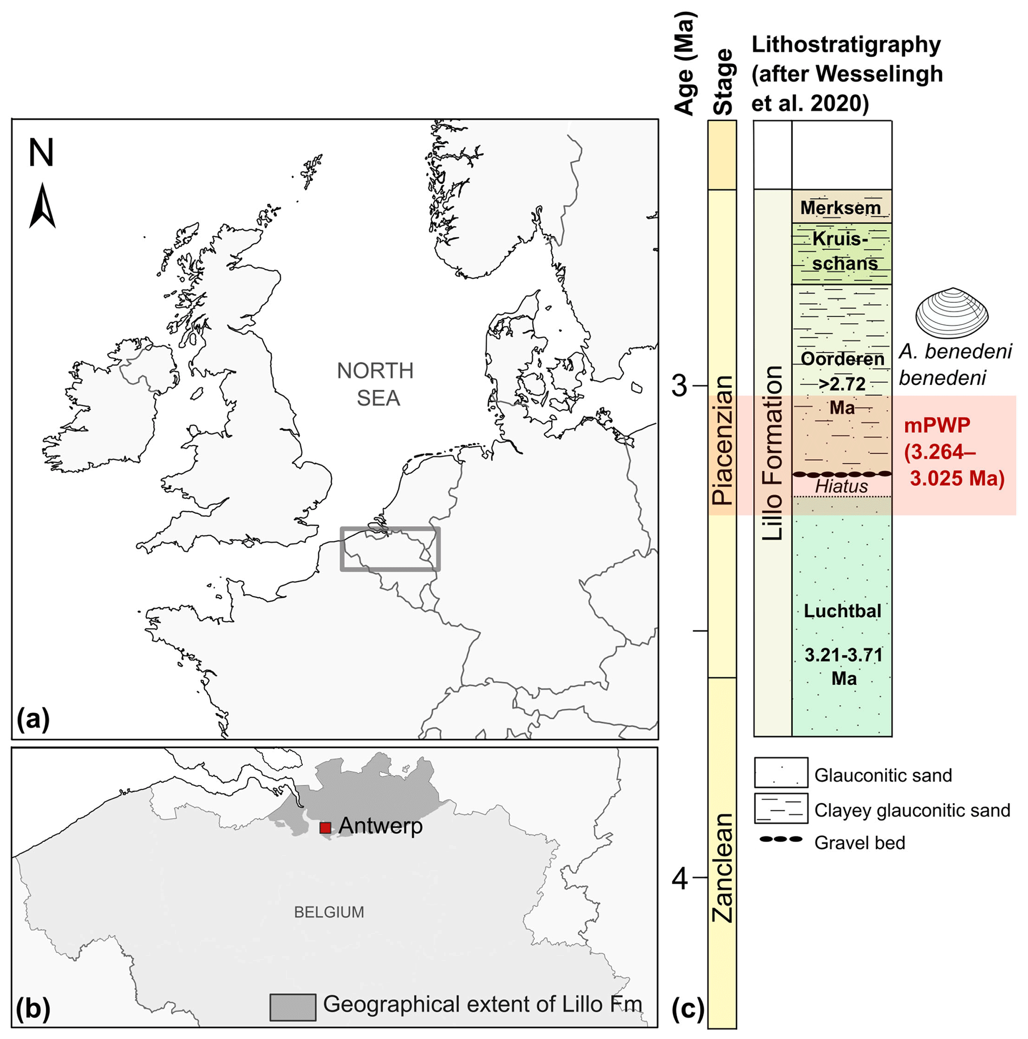
Figure 1Location of the modern North Sea basin and the stratigraphic level from which the A. benedeni benedeni specimens originated. (a) Overview map of the location of Belgium and the present-day extent of the North Sea within northwestern Europe. The dark rectangle indicates the location of map (b). Adapted after Louwye et al. (2020). (b) The geographical extent of the Lillo Formation in Belgium, after Louwye et al. (2020), and the location of the city of Antwerp. (c) Lithological column of the Lillo Formation and its members with their chronostratigraphic position, after Wesselingh et al. (2020). The Oorderen is drawn here in its longest possible range of deposition, bound by the age of the underlying Luchtbal Member (< 3.21 Ma) and biostratigraphic constraints within the Oorderen itself (> 2.72 Ma). Age boundaries for the mPWP are taken from Dowsett et al. (2010).
3.1 Light microscopy
Light microscopy was employed on all specimens to analyse the macrostructures of A. benedeni benedeni's shell and to count growth increments. Two specimens (SG-126, SG-127) were partially or fully embedded in Araldite 2020 epoxy, and high-polish thick (approximately 5 mm) sections were made, with a final polish using 0.3 µm aluminium oxide. These thick sections were viewed under a Keyence VHX-5000 digital microscope at ×250 and ×1000 magnification. Light microscopy composite images were made with the Fiji stitching ImageJ plugin (Preibisch et al., 2009). These composites were used to count the growth increments. The macrostructural layers were identified and named following Bieler et al. (2014), where M+ and M− denote layers external and internal relative to the pallial myostracum (M) (Fig. 2). The equivalent of these labels to another common naming scheme (Popov, 1986; Milano et al., 2017) is shown in Fig. 2d.
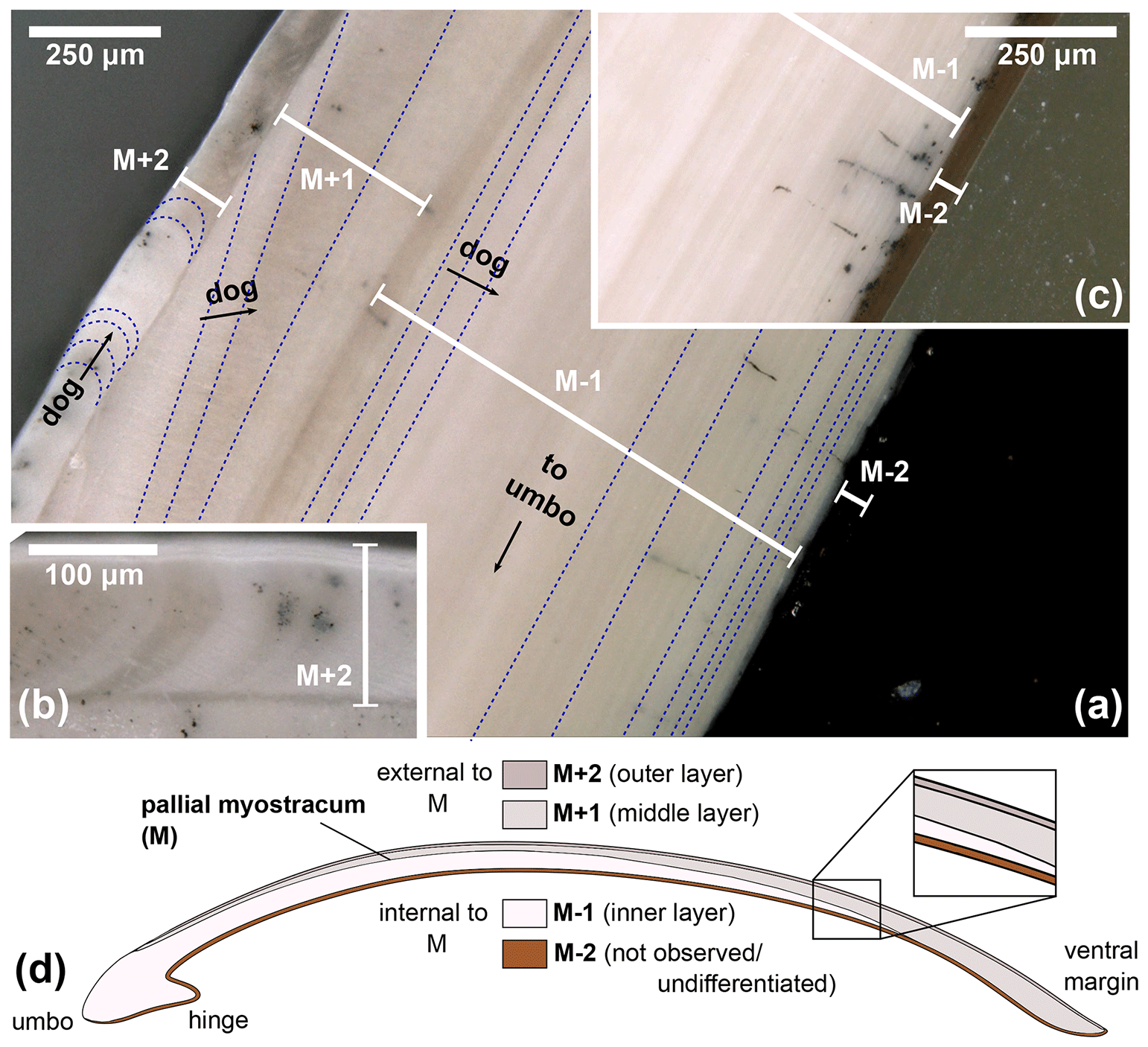
Figure 2Digital microscopy images of shell layers in the A. benedeni benedeni shells. Layers are marked M+2 to M−2; growth increments are indicated with dark blue dotted lines; dog – direction of growth. (a) Section of SG-127 indicating four layers, magnification of ×250. From outer to inner shell, these are layer M+2 with crescent-shaped growth increments; layer M+1 with low-angle growth increments and prism-like crystals parallel to the layer thickness; layer M−1 with horizontal, parallel growth increments; and layer M−2, dark brown with horizontal, parallel growth increments (difficult to see in image a due to a similar tone to the background). (b) Section of SG-126 showing a part of layer M+2 in more detail, magnification of ×500. (c) Section of SG-126 showing a part of layer M−2 at a better contrast, magnification of ×250. (d) Schematic overview of the four shell layers and their positions relative to each other and the pallial myostracum (M). In brackets is the equivalent of the layer name in the terminology of Popov (1986, 2014).
3.2 X-ray diffraction
To check for diagenetic remineralisation of original aragonite into secondary calcite, powder X-ray diffraction (XRD) analysis of a representative section of one A. benedeni benedeni specimen (SG-125) was carried out on a Bruker D8 Advance diffractometer at Utrecht University. The A. benedeni benedeni pattern was compared to XRD spectra of pure aragonite and calcite samples. The calcite spectrum was recovered from the RRUFF database (Lafuente et al., 2015; RRUFF ID: R040070). For the pure aragonite spectrum, 1.12 g of shell from a modern common cockle (Cerastoderma edule) collected at the North Sea coast near Hoek van Holland (51∘59′14′′ N, 4∘05′56′′ E) was prepared and measured under the same conditions as the fossil samples. Further measurement details are found in Appendix A1 in Table A1.
3.3 Micro-X-ray fluorescence
For additional screening of diagenetic alteration, concentrations of major and trace elements (including Fe, Mn and Sr) in the three specimens of A. benedeni benedeni (SG-125, SG-126, SG-127) were determined using non-destructive, energy-dispersive micro-X-ray fluorescence (μXRF) analysis. A benchtop Bruker M4 Tornado μXRF scanner was used for this, available at the Analytical, Environmental, and Geochemistry Research Group (AMGC) of the Vrije Universiteit Brussel (Brussels, Belgium). Online calibration (initial quantification) of the spectra was done with the matrix-matched standard BAS-CRM393 (Bureau of Analysed Samples, Middlesbrough, UK) in the M4 software (de Winter et al., 2017a). Following this, an offline calibration was carried out using a set of matrix-matched carbonate standards (Vellekoop et al., 2022). Further details are found in appendix A2. Several line scans were made per shell, after which elemental concentrations were calculated for the entire shell.
3.4 Electron backscatter diffraction
To map potential early diagenesis that was not detected in bulk XRD or μXRF analysis, as well as to determine which microstructures are present in A. benedeni benedeni, electron backscatter diffraction (EBSD) was carried out on thin sections (ca. 40 µm) of all three specimens. EBSD involves the diffraction of electrons, generated by a SEM-based electron beam, off the crystal planes of a sample, forming a diffraction pattern related to the crystal lattice parameters. This allows for the precise determination of crystal orientation, shape, and size (Cusack, 2016). EBSD analysis was carried out using an Oxford Instruments Symmetry EBSD detector attached to a Zeiss Gemini 450 SEM at Utrecht University. Thin sections of the samples were mechanically polished with 0.3 µm aluminium oxide suspension and finished with chemical Syton® polish. The thin sections were covered with a thin (several nm) carbon coating to keep charge build-up during the measurements at a minimum. Beam and map acquisition settings (voltage, beam current, dwell time, step size, high/low vacuum) were varied to obtain the optimal results for each map; the acquisition settings for the map shown here are indicated in Fig. 5. Data processing was done in the Oxford Instruments AZtecCrystal software. Data clean-up consisted of wild spike removal followed by filling in unclassified areas using an iterative nearest neighbour procedure from eight down to six nearest neighbours. The grain boundary threshold was set to 10∘. Contoured pole figures were plotted to visualise the main crystallite orientations (Fig. 5f). For these pole figures, multiple-of-uniform-density (MUD) values were calculated. The MUD value is an indication of the degree of clustering of the poles relative to a random distribution: the higher the MUD, the stronger the co-orientation (or preferred orientation) of the crystals.
3.5 Stable isotope analysis
3.5.1 Sample preparation
Samples of approximately 100–300 µg each were taken from the outer surface of two specimens (SG-126 and SG-127) by drilling into it from the exterior along commarginal paths. Specimen SG-125 was not sampled for isotope analysis as there was too little material left following XRD analysis. A Dremel hand-held drill was used, which was equipped with a tungsten carbide drill bit of 0.8 mm diameter (Fig. B1). During sampling, care was taken not to drill too deep, as this would lead to mixing of material from different shell layers that was precipitated at different points in time (Fig. B2, see also Sect. 4.1.1). The distance from the umbo to the sample track at the axis of maximum growth was measured in planar view with digital callipers (Fig. B1, Table B1). The entire shell height of specimen SG-126 was sampled (Fig. B1a). A total of 55 samples were taken from specimen SG-126, and a total of 30 samples were taken from specimen SG-127 (Fig. B1b). The sampling resolution was 0.10 to 1.07 mm (mean: 0.48 mm, 1σ: 0.24 mm; no significant difference between the two specimens, p>0.05). Samples were not homogenised prior to analysing.
For stable isotope analysis, multiple measurements were carried out on material from each drilled path. For clarity, the following terminology is used: one “sample” refers to the total powder amount that was drilled in one sample track, which runs parallel to the growth increments. One sample therefore represents a certain amount of time. One “aliquot” represents a small amount of powder taken from a “sample” which was then analysed for stable isotopes. One “measurement” refers to the measurement of one such aliquot. Multiple measurements were taken from a single sample. “Replicates” and “duplicates” refer to different aliquots taken from the same sample.
3.5.2 Oxygen isotope mass spectrometry
Drilled samples from specimen SG-126 were first analysed for carbonate oxygen isotopes (δ18Oc) on a Thermo Scientific GasBench II gas preparation system coupled to a Thermo Scientific Delta V isotope ratio mass spectrometer; 50–100 µg of powdered material was weighed for each sample and standard. Two in-house standards, Naxos marble and Kiel carbonate, were used. Their accepted values are given in Table B2. Each sample was flushed with helium for 5 min to remove atmospheric air. The samples were reacted with 103 % phosphoric acid at 70 ∘C. A Naxos standard was measured approximately every 10 samples during the run. From the bivalve samples, every 10th sample was weighed in duplicate. These duplicates were measured at the end of the run. The carbon isotope data (δ13Cc) are reported here only when it is relevant for the reproducibility of the analyses. Sample δ18Oc data were corrected for intensity-dependent fractionation using a linear regression between δ18ONAXOS and mass 44 intensity (Fig. B3). Standard deviations and uncertainties were calculated after this correction was carried out. No significant change in the Naxos standard values over time (also called “drift”) was observed during the measurement. The δ18Oc and δ13Cc data are reported relative to Vienna Pee Dee Belemnite (VPDB). The internal standard deviation of conventional stable isotope analyses was 0.04 ‰ (1σ) for δ13C and 0.06 ‰ (1σ) for δ18Oc (averaged over all measurements, n=64). External reproducibility was 0.05 ‰ for δ13C and 0.07 ‰ for δ18Oc based on repeated measurements of the Naxos standard (N=11). The Kiel carbonate standard showed external reproducibility of 0.09 ‰ for δ13C and 0.06 ‰ for δ18Oc (N=4).
3.5.3 Clumped isotope mass spectrometry
Clumped isotope analysis on carbonate involves analysing the abundance of 18O–13C bonds. The deviation of the occurrence of these heavy 18O–13C bonds from the expected stochastic distribution is thermodynamically determined and thus independent of the isotopic composition of oxygen of the seawater (δ18Osw) and carbon of the dissolved inorganic carbon (δ13C) (Ghosh et al., 2006; Schauble et al., 2006). This 18O–13C deviation is termed Δ47. Clumped isotope values (Δ47) were analysed using a Kiel IV carbonate device coupled to a Thermo Scientific MAT 253 Plus isotope ratio mass spectrometer (available at Utrecht University) with a long-integration dual-inlet (LIDI) workflow (Hu et al., 2014; Müller et al., 2017) and following the protocol described by Meckler et al. (2014). For specimen SG-126, analysis was focussed on samples with δ18Oc values in the ranges 2.0 ‰–3.3 ‰ (close to the maximum) and 0.4 ‰–1.2 ‰ (close to the minimum), based on the previously measured aliquots (Sect. 3.5.2). From specimen SG-127, all samples were analysed; 75–95 µg of powdered material was weighed out. Carbonate standards of similar weight were measured in an approximately 1:1 ratio to the standards in each run (22 samples, 24 standards; Kocken et al., 2019). ETH-3 was measured more often as it is closest in composition to the samples (Kocken et al., 2019). These standards were two control standards – Merck CaCO3 (synthetic; product code 1.02059.0050) and IAEA-C2 (Bavarian travertine) – as well as ETH-1, ETH-2, and ETH-3 (Bernasconi et al., 2018, 2021). Their composition is given in Table B2. The ETH standards, which have varying Δ47, δ18Oc, and δ13C compositions, were used to transfer the sample Δ47 values to the ICDES-90 reference frame (Bernasconi et al., 2021). Merck and IAEA-C2 were not involved in data processing (treated as samples) but used to assess long-term measuring uncertainty.
Carbonates were reacted with 105 % phosphoric acid at 70 ∘C. The produced CO2 gas was purified through two cryogenic traps (−170 ∘C) and a Porapak trap (−50 ∘C). It then entered the mass spectrometer, and masses 44–49 were measured against a reference gas (δ18O = −4.67 ‰, δ13C = −2.82 ‰). To correct for negative intensity baseline in the Faraday cups of the mass spectrometer, we performed scans of the shape of the mass spectrometry peaks using reference gas measurements before each run. The baseline on masses 47, 48, and 49 was identified and corrected by regressing the size of the negative intensity outside the peak against intensity of mass 44 (He et al., 2012). The calculated δ values were then corrected for 17O using the values presented in Brand et al. (2010). The Δ47 values were calculated and averaged over the 40 pulses as per the LIDI system. Correction of raw Δ47 values to I-CDES values (Bernasconi et al., 2021) was done in two steps. Initially all measurements are corrected using bracketing ETH-3 measurements in order to correct for variability during single runs (i.e. over the span of several hours). The offset of these bracketing ETH-3 raw Δ47 values from their I-CDES values is added to the samples. In a second step an empirical transfer function (ETF) was constructed by regressing the raw ETH-1, ETH-2, and ETH-3 values over their accepted Δ47 values and using the resulting linear regression line to transfer the sample Δ47 values to the I-CDES90 ∘C reference frame (Fig. B4). For the ETF, 403 ETH standards from multiple runs measured over the span of two months were used for linear regression (53 ETH-1, 64 ETH-2, 286 ETH-3; Fig. B5).
The δ18Oc and δ13C data of the same measurements were corrected through a 15-point running average based on the ETH standards, in order to eliminate long-term trends present within the δ18Oc and δ13C raw data. The δ18Oc and δ13C data from three runs were not used for the running average correction nor were they used in the δ18Oc records of A. benedeni benedeni. These runs show large deviations from expected values and exhibit a strong a correlation between δ18Oc and δ13C (runs 466, 468, 489; these runs are marked in Fig. B5). It seems that mass-dependent fractionation occurred during the gas preparation. The Δ47 results appear not to have been influenced by this fractionation as is evidenced by the measured standards, which show no systematic Δ47 offset (Fig. B5). Inclusion of Δ47 values from these runs did not significantly alter the temperature reconstructions beyond decreasing the confidence level on the results. Final δ18Oc and δ13C values were reported relative to VPDB. Samples that showed a strong drift during the 40 LIDI measurement pulses, had a low intensity, a high standard deviation, or showed signs of contamination, were deemed unreliable and were removed from the dataset. The intensity cut-off was < 9.0 V. The cut-off for standard deviations in Δ47 data within the 40 measurement pulses was > 0.10 ‰ for both standards and samples. Contamination evident from increased intensity on the mass 49 cup was quantified using the 49 parameter – the ratio between mass 49 and mass 44 intensities – and a cut-off of > 0.1 ‰ was used for standards and > 0.2 ‰ for samples. After removing erroneous samples, 103 sample measurements remained. The external reproducibility for the clumped isotope analyses was 38 ppm for IAEA-C2 (n=23) and 60 ppm for Merck (n=15). The external reproducibility of IAEA-C2 was used as the standard deviation on Δ47 for the samples, as it is closer in composition to the samples than Merck (Fig. B5). After corrections, most of the Δ47 data ranged between 0.55 ‰ and 0.70 ‰ for both specimens.
For oxygen isotopes, the external reproducibility of the standards does not reflect the reproducibility of the samples based on duplicate measurements. The samples from each sampling track were not homogeneous, as they likely contain multiple thin growth increments and were not homogenised after drilling. Therefore, different aliquots from the same sample sometimes resulted in considerable differences when measured, in both the GasBench and the MAT 253 PLUS analyses. Instead of using the external reproducibility on the Naxos standard, the uncertainty on the shell data was determined as follows: for each sample for which replicates were analysed, the standard deviation of these replicates results was taken, and all these standard deviations were averaged. To this goal, δ18Oc data from GasBench and MAT 253 PLUS analyses were combined. This resulted in an uncertainty of 0.15 ‰ for SG-126 (n=28 replicates). There were not enough duplicate δ18Oc measurements for SG-127, so the value of 0.15 ‰ was also applied to this specimen.
3.6 Palaeotemperature reconstruction
All Δ47 values were compiled and converted to a mean annual temperature (MAT) using the temperature transfer function of Meinicke et al. (2020, 2021):
This temperature transfer function is based on foraminifera and therefore more suited to the low temperature range in which bivalves live. Recently, it was shown that this clumped isotope thermometer yields the most accurate temperature reconstructions in aragonitic bivalves (de Winter et al., 2022). Since the temperature function for Δ47 is not linear, errors associated with the Δ47 data were propagated using a Monte Carlo simulation (n = 105) of uncertainty in slope and intercept of the temperature transfer function as well as measurement uncertainty on Δ47 values assuming a normal uncertainty distribution. The standard deviation, standard error, and 95 % confidence level were then calculated from this normally distributed simulated temperature dataset. Uncertainties on temperatures were calculated after temperature conversion. Since the temperature transfer function for clumped isotopes is not linear, this introduces a bias, specifically towards warmer temperatures. The temperature means were therefore calculated from averaging the Δ47 values instead, and the Monte Carlo-generated errors were transferred to these mean temperatures.
The δ18O of the seawater (δ18Osw) was calculated from Δ47-based MAT and δ18Oc data using the temperature transfer function for aragonite of Grossman and Ku (1986), modified by Dettman et al. (1999):
VSMOW stands for Vienna Standard Mean Ocean Water. This average δ18Osw, the Δ47-based MAT, and minimum and maximum δ18Oc values were then re-inserted into this equation to obtain δ18Oc-based summer and winter temperatures.
3.7 Growth models
To gain insights into the nature of the growth of A. benedeni benedeni, two types of growth models were fitted to the growth data of specimen SG-126: the Von Bertalanffy growth function (VBGF), a logarithmic model, and the Gompertz equation, a logistic model. Both are widely used for estimating and analysing growth in modern species (Lee et al., 2020). The built-in nls function in R (R Core Team, 2021) was used to fit the data to both growth functions (see code availability). The VBGF and the Gompertz equations are restrictive in terms of how much their shape can change, and more sophisticated approaches are available today (Lee et al., 2020). However, as this study has only one specimen available for growth model fitting, and since it concerns a fossil species, we believe that this simple approach is appropriate. The VBGF has the form of Eq. (3), where H is the body size of the specimen at time t (here: shell height measured as distance from umbo), Hasymp is the asymptotic height (i.e. the theoretical maximum shell height), k is the growth coefficient, t is the time (here: in years), and t0 is the theoretical time where H equals 0.
The Gompertz equation has the form of Eq. (4):
where H is again the shell height at time t, Hasymp is the theoretical maximum shell height, and b and c are coefficients. Each parameter, its associated standard error (SE), and p value were calculated.
4.1 Light microscopy
4.1.1 Structural analysis
Angulus benedeni benedeni shells consist of four layers, M+2 to M−2 (Fig. 2), labelled from the outer to the inner surface. M+2 and M+1 are located outside of the pallial myostracum and form the outer shell layers. M+2 is a thin (ca. 100 µm) white-to-grey coloured layer with crescent-shaped growth increments. M+1 is a ca. 200 µm thick layer (measured at the thickest point, halfway along the shell height) with low-angle growth increments and white–beige in colour. M−1 and M−2 are located inside of the pallial myostracum and form the inner shell layers. M−1 is a thick (ca. 1000 µm) layer with clear growth increments parallel to the layer boundaries and a white–beige colour. M−2 is a thin (ca. 50 µm) brown-coloured layer with horizontal, parallel growth increments similar to M−1.
4.1.2 Growth increments
In specimen SG-126, a maximum of 115 growth lines were counted in layer M−1 at the hinge (Fig. 3a, c). In specimen SG-127, a maximum of 130 growth lines were counted just ventral of the hinge (Fig. 3b, c), also in layer M−1. The growth lines were not all clearly visible, and in some areas in the shell, fewer growth lines could be discerned. As it was deemed easier to miss some growth lines due to the limited resolution than to overestimate the number, the microscope images with the maximum counted number of growth lines are shown here. Although still an underestimate, these are thought to be the best estimate of the actual number of growth lines.
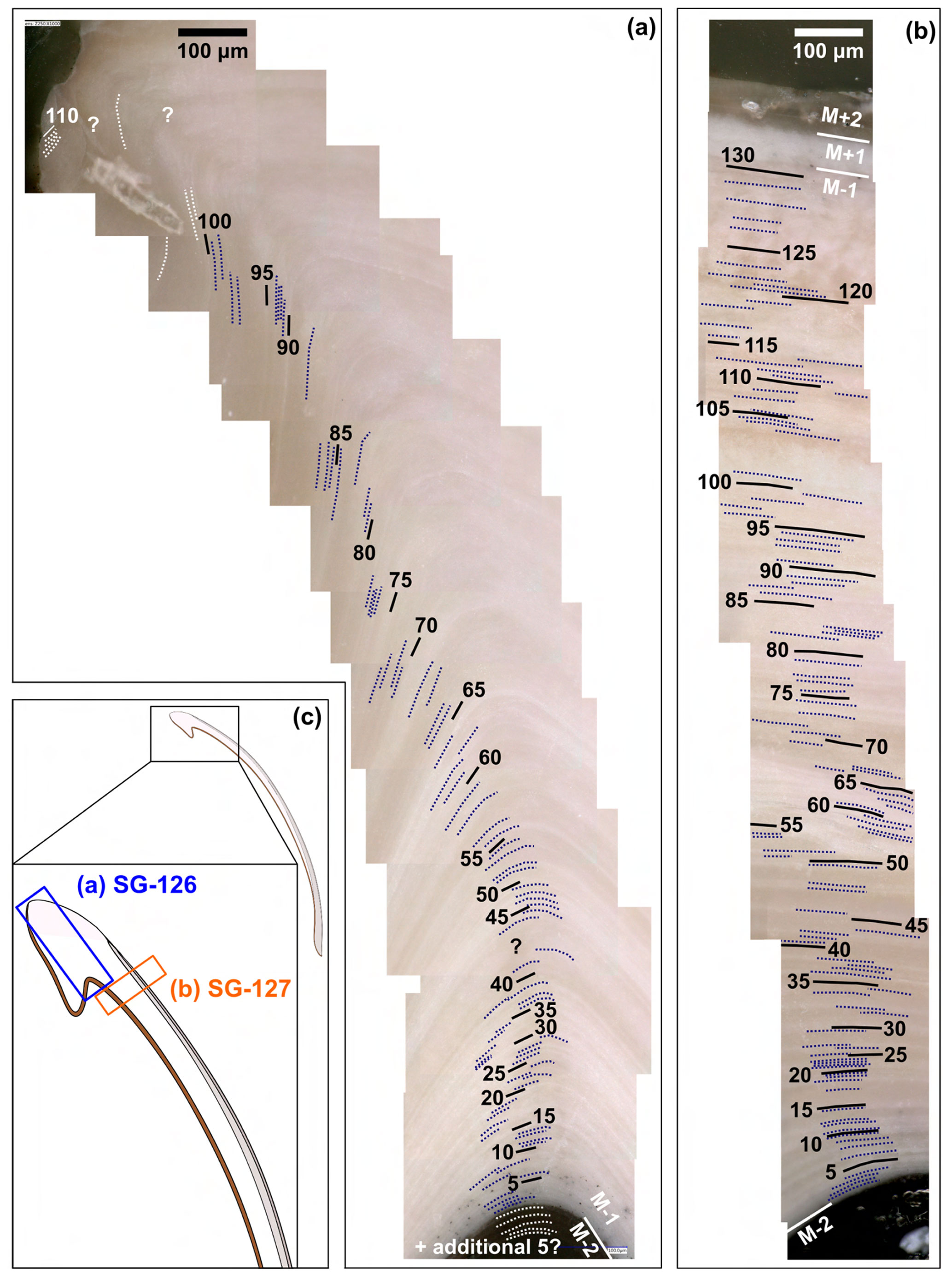
Figure 3Growth lines in the A. benedeni benedeni specimens. (a) Counted growth lines in specimen SG-126, 115 in total. Counted in shell layer M−1. (b) Counted growth lines in specimen SG-127, 130 in total. Counted in layer M−1. (c) Schematic figure of the shell indicating where the growth lines were counted.
4.2 X-ray based analyses
X-ray diffraction analysis (XRD) and micro-X-ray fluorescence (μXRF) point analysis indicate that the aragonite in the shells of A. benedeni benedeni was not diagenetically altered. XRD analysis revealed that the shell of A. benedeni benedeni consists of 100 % original aragonite, as its spectrum is identical to that of pure aragonite (Fig. 4a). Micro-X-ray fluorescence (μXRF) point analysis supports this interpretation, as the specimen is high in Sr while low in Fe and Mn (Fig. 4b). Higher concentrations of Fe and Mn and lower concentrations of Sr in fossil carbonates are generally associated with pore water interaction during diagenetic alteration (e.g. partial recrystallisation) of the carbonate (Brand and Veizer, 1980; Al-Aasm and Veizer, 1986; Hendry et al., 1995). The absence of high Fe and Mn concentrations and presence of high Sr suggest that this process did not take place in these specimens.
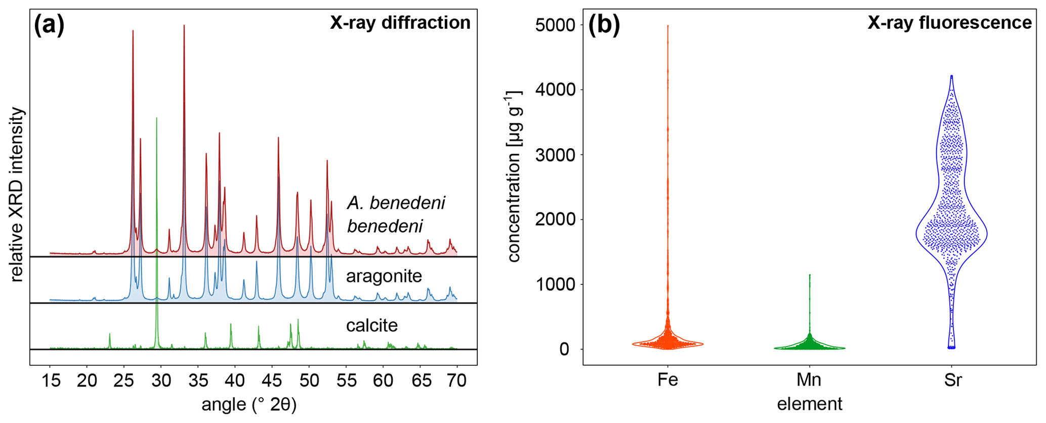
Figure 4X-ray-based analysis results to assess diagenetic alteration in the specimens. (a) X-ray diffraction analysis of A. benedeni benedeni compared with patterns of pure aragonite and calcite, indicating an aragonitic composition of the shell. (b) Violin plot showing the results of the X-ray fluorescence analysis of A. benedeni benedeni for the elements Fe, Mn, and Sr. The “violin” shape depicts the kernel density function for the elemental concentration, plotted vertically and mirrored. The specimen is high in Sr and shows a broad distribution within these higher values. While there are some data points with high Fe and Mn values, the distribution is strongly skewed towards low values, suggesting overall low Fe and Mn values.
4.3 Electron backscatter diffraction
4.3.1 Diagenesis assessment
Electron backscatter diffraction (EBSD) analysis shows no evidence of diagenetic alteration in the shells. In the EBSD maps, 0 % to 0.2 % of the area was initially classified as calcite. Upon inspection, these “calcite” grains are wild spikes that were subsequently removed in the data clean-up (Fig. C1). There was no local secondary mineral growth visible in any map (e.g. Fig. 5b–e), which would have presented itself as larger crystals (“blocky calcite”) that do not follow the surrounding structures (Cusack, 2016; Casella et al., 2017). The pole figures show a clear preferred orientation (Fig. 5f), which is indicative of original growth structures (Casella et al., 2017).
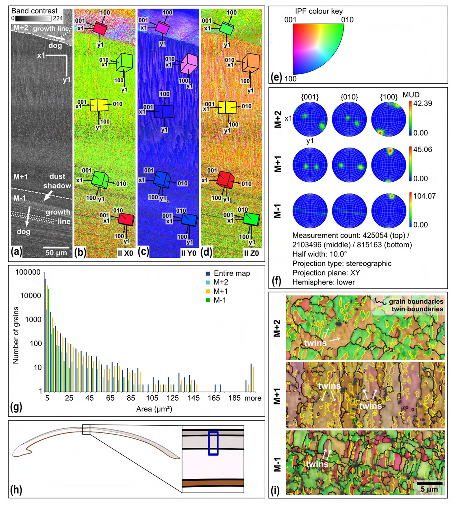
Figure 5EBSD map of specimen SG-127. Map acquisition specifics: 20 kV, high vacuum, 0.2 µm step size. (a) Band contrast map with scale, orientation, growth lines, direction of growth (dog), and shell layers M+2, M+1, and M−1, separated by dashed lines. (b) EBSD inverse pole figure (IPF) X map, showing grain orientations parallel to the X0 axis. Unit cells of aragonite with the most common orientations are shown, the colour of which corresponds to the colour coding of the map. (c) EBSD IPF Y map showing grain orientations parallel to the Y0 axis, with unit cells. (d) EBSD IPF Z map showing grain orientations parallel to the Z0 axis, with unit cells. (e) Inverse pole figure (IPF) colour key for the EBSD orientation maps. (f) Contoured pole figures for the three main crystallographic directions and the MUD, for the different shell layers. (g) Grain size distribution chart for the entire map and the different shell layers. Note the logarithmic y axis. (h) Schematic figure indicating the approximate location of the map on the shell. (i) Shell layers from map IPF Z zoomed in and with added grain (black) and twinning (yellow) boundaries.
4.3.2 Grain size and orientation
The aragonitic shell material is fine grained, and its crystals show a strong preferred orientation as well as twinning. Most grains have an area of a few µm2 or smaller (Fig. 5g). Layer M−1 has a narrower grain size distribution than M+1 and M+2, with no grains larger than 25 µm2 present in the analysed section. The multiples-of-uniform-density (MUD) values indicate a strong preferred orientation (Fig. 5f). Layer M−1 has an increased MUD of 104.07 compared to ca. 40 for the other two layers, indicating a stronger preferred orientation (Fig. 5f). This is due to the strong preferred orientation of the 100 axis, while the 001 and 010 axes show a weaker preferred orientation compared to the other layers. The pole plots show double maxima of the 001 and 010 axes, which rotate around the 100 axes (M+2 and M+1, Fig. 5f). This is observed in layers M+2 and M+1. In layer M−1, the 001 and 010 axes form a girdle around the 100 axis rather than two distinct maxima (M−1, Fig. 5f). The rotational 100 axis is generally oriented parallel to the growth direction. This is especially evident from the lamellae in layer M−1 of Fig. 5b–e.
The angle of ca. 64∘ between the 001 and 010 axes is characteristic of aragonite polysynthetic (110) twinning (Griesshaber et al., 2013). Calculated twinning boundaries indicate that the two dominant orientations, as indicated by the inverse pole figure (IPF) colour coding, in layers M+2 and M−1 represent twins (Fig. 5i). In layer M+1, the two dominant orientations that make up the lamellae are not a result of twinning. Instead, each of the two orientations (orange and purple) consists of their own set of twins (light and dark orange and purple, respectively; Fig. 5i).
4.3.3 Microstructures
Within the EBSD maps, several different structures are observed (Fig. 6). Layer M+2 consists of a compound composite prismatic structure, formed by bundles of crystals that diverge from the centre of the layer (Fig. 6a) (Popov, 2014). Layer M+1 consists of a crossed lamellar structure. This is indicated by two sets of crystal orientations that are oriented perpendicular to the growth lines and that alternate and interfinger, similar to a zebra pattern (Fig. 6b) (Popov, 2014; Crippa et al., 2020). Layer M−1 shows multiple structures. In the hinge region, a hatched pattern is visible (Fig. 6c), corresponding to a complex crossed lamellar structure (Popov, 2014). In other parts of M−1, elongated, columnar crystals with their long side oriented parallel to the growth direction are observed (Fig. 6d), indicative of a prismatic structure (Popov, 2014). Around this prismatic structure, there are small grains with no clear preferred shape orientation (Fig. 6d). This has been interpreted as a homogenous structure (Popov, 2014). However, it might also be a different structure that cannot be analysed at this resolution due to the fine-grained nature of the aragonite. Layer M−2 was not captured on any EBSD map.
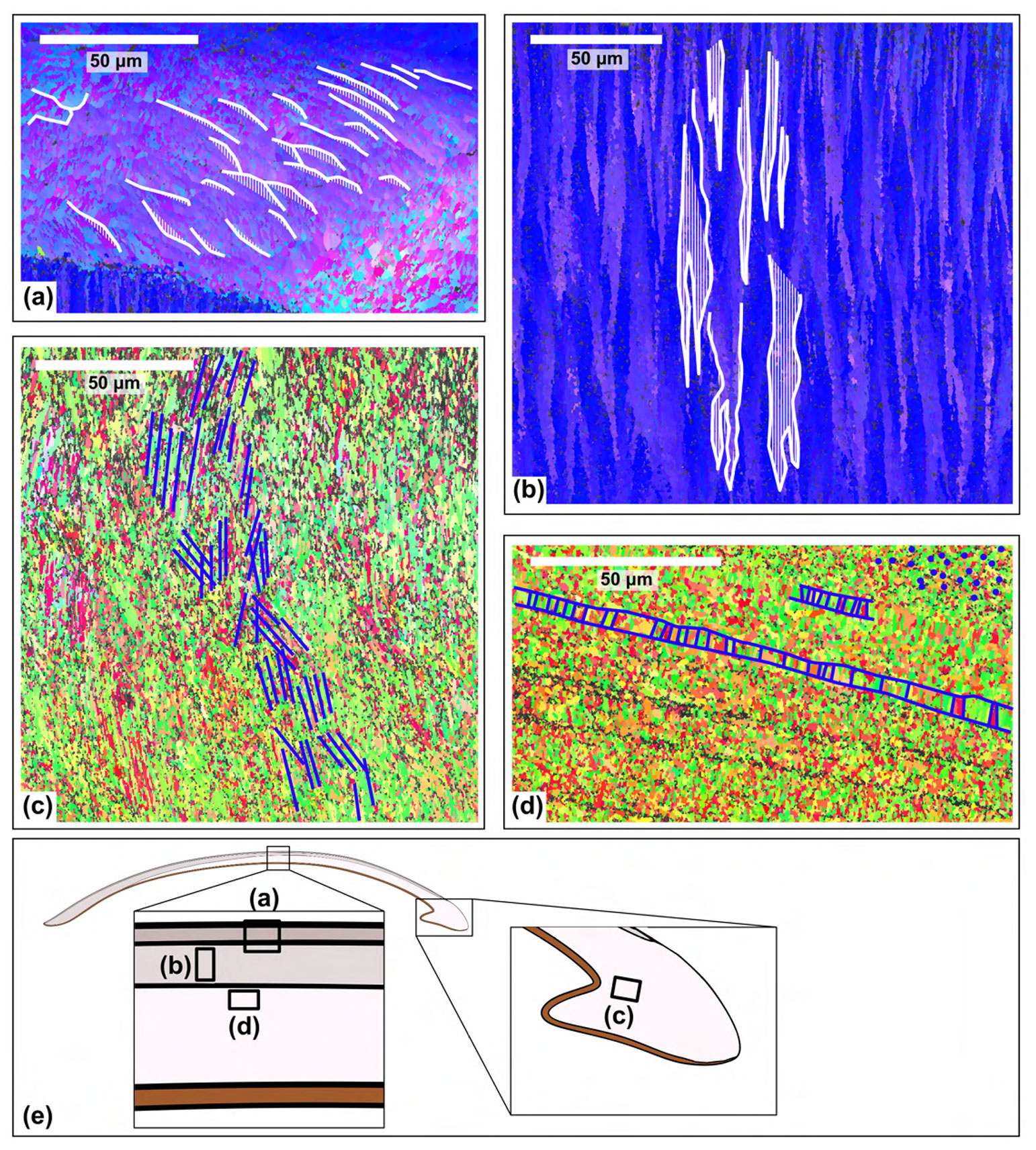
Figure 6Different shell structures identified in the EBSD maps of specimen SG-127. (a) Compound composite prismatic structure in layer M+2. (b) Crossed lamellar structure in layer M+1. (c) Complex crossed lamellar structure in layer M−1 at the hinge of the shell. (d) Prismatic structure in layer M−1. There are also areas in this layer (e.g. top right in panel d) without a clear grain shape structure, which are interpreted as a homogeneous structure. (e) Schematic figure of the shell indicating the approximate location of the maps.
4.4 Stable isotope analysis
4.4.1 Oxygen isotopes
The δ18Oc data of specimens reveal sinusoidal records that range between +0.3 ‰ and +3.3 ‰ (Fig. 7a, b) and suggest multi-annual growth, with δ18Oc peaks corresponding to winters and valleys corresponding to summers. Specimen SG-126 shows at least 8–9 years of growth (Fig. 7a). The first and last years of this specimen may not have been recovered during sampling, as the first and last few millimetres were not sampled. In addition, the sampling resolution was likely too coarse to capture all years in the ontogenetically oldest section of the shell, as growth increments generally become thinner with age. In SG-126, high δ18Oc values generally correspond to darker bands and vice versa, which suggests that the dark–light couplets represent the winter and summer seasons. The δ18Oc variability decreases near the ventral margin of the shell. The sampled section of SG-127 shows six cycles in δ18Oc values (Fig. 7b). In contrast to SG-126, the relationship between δ18Oc value and shell colour is not consistent. There are many thin light and dark bands on SG-127, and samples likely contain material from both light and dark bands (Fig. 7b; not all indicated on Fig. 7b as the exact location relative to the samples was not determined).
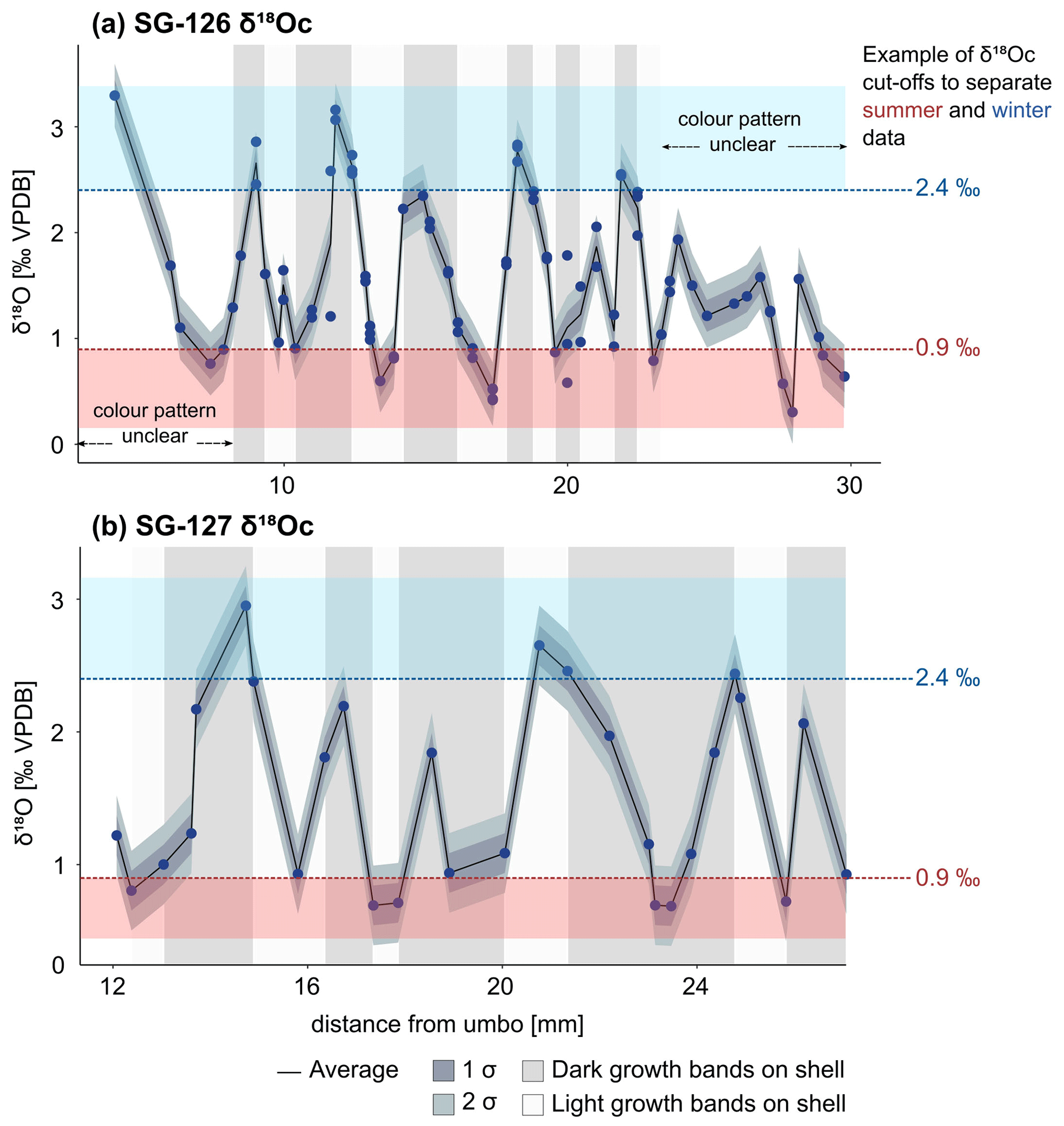
Figure 7δ18Oc records of the A. benedeni benedeni shells, plotted relative to the distance from the umbo. (a) Record of specimen SG-126, consisting of 55 samples each measured 1 to 3 times. (b) Record of specimen SG-127, consisting of 30 samples. The average was calculated from the different measurements of a single sample. If there was just one measurement, that value was taken; 1 and 2 standard deviations are plotted around the average. The standard deviation was calculated as described in Sect. 4.4.1 (0.15 ‰). In the background, the approximate colour of the growth band on the outer surface of the shell is indicated (see also Fig. B1). The warm and cold δ18Oc “bins” are marked in red and blue bands. These bins encompass all data points below 0.9 ‰ and above 2.4 ‰. See also Sect. 3.4.3 and Fig. 9. Raw data are plotted in Fig. B6.
4.4.2 Growth curves
A growth curve was reconstructed for the specimen SG-126 using the δ18Oc record (Fig. 8a–b). This was not done for specimen SG-127 as only a small section of the entire shell was sampled. As there appear to be several smaller fluctuations in the δ18Oc record, a “year” was defined as a fluctuation that consists of 2 or more data points. This leaves out a small peak at 9.97 mm from the umbo and a larger peak at 21.02 mm (Fig. 8). An alternative growth model that counts this larger peak as a year is shown in Fig. B7. Figure 8 shows the fitted Von Bertalanffy and Gompertz growth models. For the Von Bertalanffy model, the parameters Hasymp, k, and t0 were estimated to be 52.35 ± 7.64 SE (p<0.05), 0.09 ± 0.02 SE (p<0.05), and 0.03 ± 0.16 SE (p≫0.05) respectively. Hasymp is the estimated maximum shell height in millimetres that A. benedeni benedeni would have reached, ca. 52 mm. The interpretation of growth coefficient k is problematic, and besides having a large standard error and low confidence, t0 is merely a mathematical artefact that does not have any biological meaning (Lee et al., 2020). For the Gompertz model, parameters Hasymp, b, and c were estimated to be 34.11 ± 1.98 SE (p<0.05), 2.58 ± 0.14 SE (p<0.05), and 0.29 ± 0.03 SE (p<0.05), respectively. The Gompertz model thus suggests a shorter maximum shell height of 34.11 mm. The standard error on the residuals is 0.51 for the VBGF and 0.63 for the Gompertz equation. The R2 value for both fits is 0.99, but as both functions are non-linear, this is not a reliable indicator of goodness of fit (Spiess and Neumeyer, 2010). This rather preliminary growth model fitting suggests a maximum size of A. benedeni benedeni of 34–52 mm.
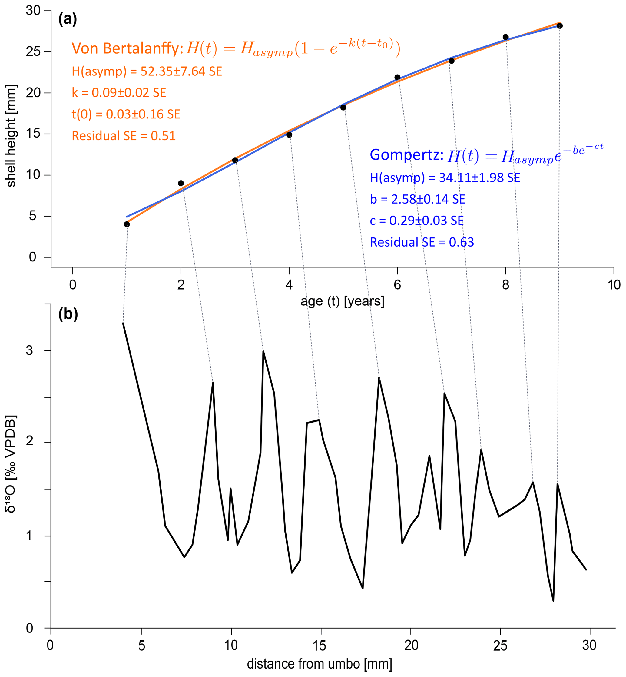
Figure 8Growth curves for specimen SG-126. (a) Growth curves constructed by inserting the counted years versus distance-from-umbo data points into two different fitting algorithms: the asymptotic Von Bertalanffy growth function and the logistic Gompertz function. (b) δ18Oc record with the inferred growth years marked by lines connecting to plot (a).
4.4.3 Δ47 and palaeotemperature
A mean annual temperature (MAT) of 13.5 ± 3.8 ∘C has been calculated through averaging all Δ47 values and converting this average to a single temperature, with the 95 % confidence level (CL) determined through Monte Carlo error propagation. Reliable Δ47-based summer and winter temperatures could not be determined due to a limited amount of data. This issue is illustrated in Fig. 9. To obtain summer and winter datasets, we selected samples with respectively low and high δ18Oc values from both specimens and subsequently averaged their associated Δ47 values (similar to the “optimisation” approach as discussed in de Winter et al., 2021a). This grouping by δ18Oc value is necessitated by the large uncertainty on individual Δ47 measurements, which means that Δ47 data points cannot be split into meaningful “warm” and “cold” groups directly. The choice of a cut-off value for warm and cold δ18Oc values is a trade-off between signal and noise: a cut-off close to the average δ18Oc value results in a higher sample size and a narrower confidence interval for the resulting temperature reconstruction. However, this also results in averaging samples from a large part of the year and thus a dampening of the seasonality signal. For a cut-off that only includes the lowest and highest δ18Oc values, the opposite is true. To determine whether there was an acceptable compromise between signal and noise, the average warm and cold Δ47 values and their associated 95 % confidence levels were plotted for a range of δ18Oc-based cut-offs (Fig. 9). Oxygen isotope data from both specimens were combined to improve the statistics. Combining δ18Oc and Δ47 data to reconstruct seasonality is the recommended strategy when a sampling resolution of 1 data point per month cannot be obtained, as was the case on the small shells of A. benedeni benedeni (Zhang and Petersen, 2023).
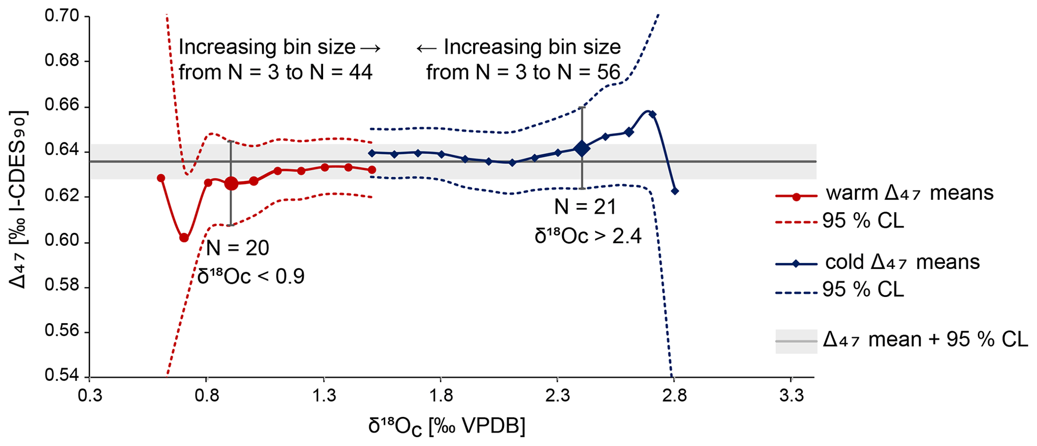
Figure 9Overview of averages (round and diamond symbols) and 95 % confidence intervals (dashed lines) for different-sized groups of summer and winter Δ47 aliquots. Sizes of groups increase towards the middle of the plot. The larger symbols with vertical error bars highlight the issue of having insufficient aliquot measurements. The bin sizes are small, and so they should come close to the true (non-averaged) seasonality. However, the number of aliquots is reduced to ca. 20 at this point. This translates to large errors, making these cold and warm averages statistically indistinguishable from each other.
Figure 9 shows that an acceptable compromise between signal and noise to resolve seasonality is not possible with the limited amount of data obtained here. The δ18Oc cut-offs for < 0.9 ‰ and > 2.4 ‰ are highlighted to illustrate this. At these cut-off points, which are arbitrarily chosen, the number of data points (n=20 and n=21, respectively) is large enough to reduce the 95 % CL range. Further improvement within this dataset is hardly possible as the error bars plateau shortly after, corresponding to ca. n=30. However, the two datasets are not statistically different (p>0.05, Student's t test) already in sample sizes starting from 20 aliquots, due to both the wide δ18Oc range included in these cut-offs and the large 95 % CL range. Increasing the number of clumped isotope measurements that correspond to the more extreme δ18Oc values would decrease the large errors and would allow for making the cut-offs narrower. This way, they better represent the seasonal extremes. That this approach works is exemplified by the MAT of 13.5 ± 3.8 ∘C. Due to the large number of measurements (N=103), the error on this temperature has been reduced to a few degrees Celsius. The same is possible for seasonal temperatures if the dataset is large enough. Besides the large analytical error associated with clumped isotopes, seasonal variability will also add to the standard deviation on the MAT. Even with more data, the degree to which this error can be reduced is therefore limited. Clumped-isotope-based summer and winter temperatures are not calculated here and will not be discussed further, as the data generated in this study are not sufficient to do so in a meaningful way. Instead, we discuss an alternative approach to obtain seasonal temperatures below.
4.4.4 δ18Osw, δ18Oc, and temperature
The average δ18Osw is 0.10 ± 0.88 ‰ VSMOW (95 % CL), based on the average Δ47-based temperature of 13.5 ± 3.8 ∘C and the average δ18Oc of both shells combined (1.53 ± 0.015 VSMOW, 95 % CL). The Grossman and Ku (1986) equation was applied to the highest and lowest δ18Oc values and the annual mean δ18Osw to obtain winter and summer temperatures (Fig. 10a). To obtain these highest and lowest δ18Oc values, the three lowest (0.30 ‰, 0.42 ‰, 0.43 ‰) and highest (3.07 ‰, 3.16 ‰, 3.29 ‰) data points were averaged. These three points were chosen to capture the largest seasonal range that was recorded while not relying on a single measurement. This resulted in summer and winter temperatures of 18.5 ± 3.9 and 6.4 ± 3.9 ∘C (95 % CL, Fig. 10b). Note that this approach does not take into account seasonal changes in δ18Osw.
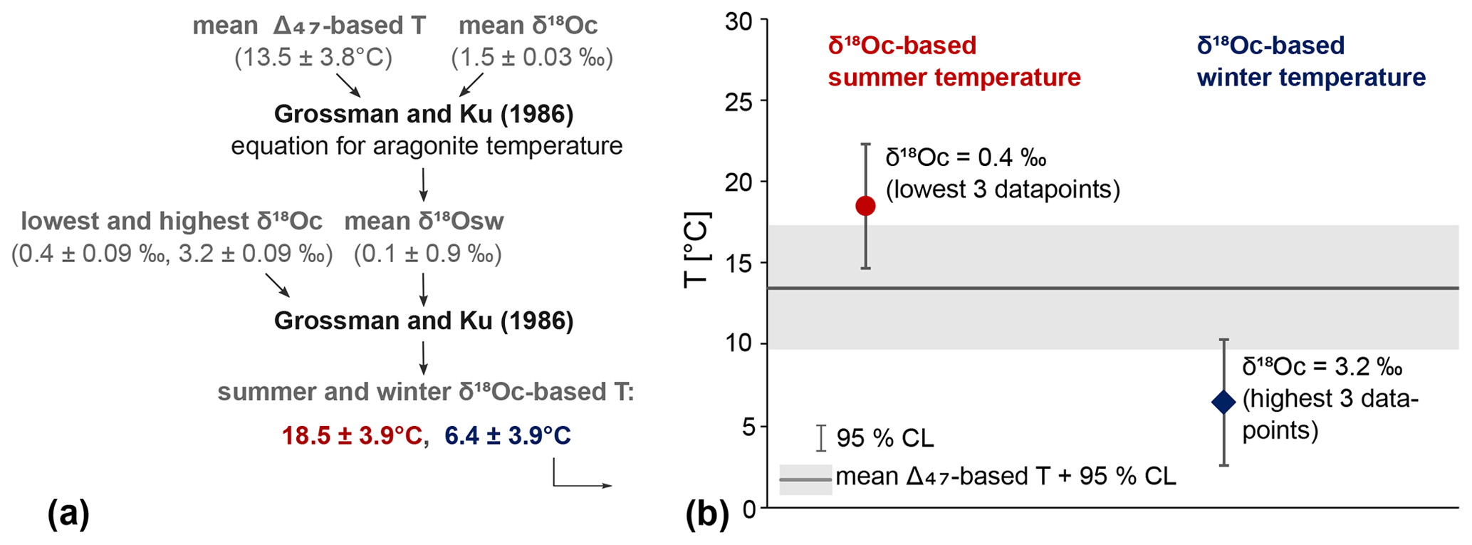
Figure 10δ18Oc-based summer and winter temperatures. (a) Schematic illustrating how the δ18Oc-based temperatures have been calculated and what values were used. All values after ± are 95 % CLs. (b) Mean δ18Oc-based summer (red circle) and winter (blue diamond) temperatures and their 95 % CL. In the background, the Δ47-based mean temperature and confidence interval is shown (grey band). The δ18Oc values used are the average of the lowest and highest three data points.
5.1 Diagenesis
No signs of diagenesis of the shells were found through micro-X-ray fluorescence (μXRF), X-ray diffraction (XRD), and electron backscatter diffraction (EBSD) analyses. The μXRF analyses indicated that the shell material was high in Sr and low in Fe and Mn; these latter two elements are regularly used to pinpoint diagenesis (Fig. 2b; de Winter and Claeys, 2017). The XRD pattern of specimen SG-125 consisted of 100 % aragonite. No blocky calcite was observed in the EBSD images of any of the three specimens (Cusack, 2016; Casella et al., 2017). This alone does not preclude diagenetic alteration, as calcite is not formed in the earliest stages of diagenesis (Cochran et al., 2010; Marcano et al., 2015; Ritter et al., 2017). Further analysis of the EBSD maps did not, however, produce any evidence for diagenetic alteration. Microstructures that are similar to those found in modern Tellinidae were observed in the EBSD maps (Popov, 2014). In altered aragonitic bivalves, the structures as observed from EBSD maps are more homogenous and have a lower MUD compared to pristine material (Casella et al., 2017; study of Arctica islandica). Even the homogeneous structure in A. benedeni benedeni (Fig. 6d) appears less chaotic than altered aragonite (Casella et al., 2017). Combined with the shallow burial depth (≤ 100 m; Johnson et al., 2022) and the unconsolidated and fine-grained nature of the surrounding sediment, this evidence suggests that no significant diagenetic alteration took place. The isotope values presented here therefore record the formation temperature of the biogenic aragonite, assuming equilibrium fractionation, and support the interpretation of the stable isotope data in this study.
Previous studies have indicated good preservation of bivalves from the Oorderen Member (Valentine et al., 2011; Johnson et al., 2022), from other members of the Lillo Formation (Johnson et al., 2022), and from the Early Pliocene Ramsholt Member of the Coralline Crag Formation (Johnson et al., 2009; Vignols et al., 2019). Pliocene shells from the North Sea basin are expected to yield reliable temperature results via geochemical analysis, as long as preservation is not obviously suspect (e.g. in the Sudbourne Member of the Coralline Crag Formation in southeastern England, whose aragonitic shells have nearly all been dissolved; Balson et al., 1993). However, it remains imperative to screen for early diagenesis when analysing shells from new localities and older stratigraphic intervals. This is especially relevant for seasonality studies. During early diagenesis, the intra-shell δ18Oc variations that reflect seasonal variability can be homogenised, dampening the original signal. Evidence that this has taken place is limited to subtle changes in scanning electron microscope images (Moon et al., 2021). To the authors' knowledge, whether these changes are detectable with EBSD has not been studied yet.
Based on the results in this study as well as practical considerations, we recommend a combination of light microscopy and trace element analysis (XRF) for diagenetic screening in general, while the addition of XRD analysis is advised only for aragonitic shells (such as A. benedeni benedeni). While EBSD is a powerful method for observing and classifying shell microstructures and assessing their preservation, its limited accessibility and comparatively time-consuming data processing renders this method somewhat unwieldy for routine preservation screening.
5.2 Angulus benedeni benedeni shell structure
The shell of A. benedeni benedeni consists of four macrolayers, of which the outer three show microstructures that were identified using EBSD. From outer (M+2) to inner (M−1), these are compound composite prismatic, crossed lamellar, complex crossed lamellar–prismatic–homogeneous (Popov, 2014). These structures have all been described previously in other tellinid genera such as Macoma, Peronidia, and the lucinid Megaxinus (Popov, 2014). Tellinidae generally have three layers, sometimes with sub-layers present. The M−1 layer in Tellinidae is usually homogeneous, as it appears to be in our specimens (Popov, 2014). Beyond this, there exists a wide range of variation in tellinid bivalve shell microstructures (Popov, 2014). Angulus benedeni benedeni is similar in structure to the closely related A. nysti (Popov, 2014). Layer M−2 was not studied with EBSD here, but light microscopy suggests that it might be structurally similar to the neighbouring M−1 layer (Fig. 2).
Aragonite polysynthetic (110) twinning – indicated by a 64∘ misorientation angle between the 001 and 010 axes – is frequently observed in bivalves (Kobayashi and Akai, 1994; Griesshaber et al., 2013; Crippa et al., 2020) and other molluscs (Schoeppler et al., 2019). It contributes to rapid shell growth as it is more efficient at filling up space than non-twinned growth (Schoeppler et al., 2019). This twinning is observed in all analysed layers of A. benedeni benedeni. As the double 001 and 010 maxima are stronger in the external layers M+2 and M+1 than in the internal layer M−1, twinning may be more significant in these two layers. This may, in turn, be linked to more rapid precipitation. This study supports previous investigations in highlighting the utility of EBSD for analysing shell structures in bivalves (Cusack, 2016; Checa et al., 2019; Crippa et al., 2020), which remains a rather new application of this technique.
5.3 Angulus benedeni benedeni growth history
Angulus benedeni benedeni experienced slower growth in winter, could live for up to a decade or longer (Figs. 7, 8), and likely reached lengths of 34–52 mm. The maximum (winter) δ18Oc values decrease, while the minimum (summer) values stay similar throughout the oxygen isotope record of specimen SG-126. This amplitude reduction may reflect growth breaks during the colder months. This is supported by the correlation of high δ18Oc values with dark growth bands on the shell's exterior (Fig. 7). Darker bands in bivalves often have high organic matter content related to decreased mineralisation rates (Lutz and Rhoads, 1980, cited in Carré et al., 2005). The pronounced ontogenetic growth rate decline that is often seen in bivalves (McConnaughey and Gillikin, 2008) is not apparent from the growth curve of specimen SG-126. The growth curve only becomes slightly less steep in the last few measured years, and there is no marked decrease in the wavelength of the δ18Oc record (Fig. 8).
Simple growth modelling has provided a preliminary range of maximum shell height for A. benedeni benedeni. The VBGF yields a higher maximum shell height estimate than the Gompertz equation (52 vs. 34 mm, respectively). Due to the nature of the respective models, the VBGF tends to overestimate the maximum shell height, while the Gompertz equation tends to underestimate it (Urban, 2002). These two estimates therefore yield a plausible range for the maximum shell height of A. benedeni benedeni. The heights of specimens SG-126 and SG-127 (30–36 mm) are close to the Hasymp of the Gompertz model, and the other specimens in the collection of the Royal Belgian Institute of Natural Sciences generally do not exceed 40 mm in height. The shape of the VBGF and Gompertz curves suggest that specimen SG-126 had not yet reached its maximum shell height. A. benedeni benedeni may have lived longer than 8–9 years.
Bivalves can form growth increments on a variety of timescales, and their growth rhythm can be influenced by solar and lunar cycles (Tran et al., 2011). The number of growth lines counted in A. benedeni benedeni was divided by the inferred age of the specimen to determine its growth rhythm. The sampled intervals span several years: around 9 years for SG-126, which represents most of the shell height, and around 6 years for SG-127, which represents only around one-third of the shell height. In both shells, 100+ growth lines were counted. In SG-126, the maximum number of years counted (9) and the maximum number of growth lines counted (115) correspond to ca. 13 growth lines per year. This is an interval of approximately 29 days, which matches the periodicity of the monthly synodic lunar–tidal cycle. However, both growth lines and years are likely to be underestimated. Their recordings are both limited by either the microscopy or the sampling resolution. Additionally, the shells likely experienced winter growth stops, so the growth increments do not record a full year. It is difficult to put constraints on these uncertainties due to limited data availability. These uncertainties work in different directions (underestimating the number of years results in more time represented within a growth increment; underestimating the number of growth increments and the amount of time missing due to winter stops results in less time within a growth increment). As two out of three factors push the duration of a growth increment towards lower values, each increment may represent less than 29 days. This fits with the nature of lunar–tidal forcing. There is little difference between the two spring–neap cycles within a monthly cycle (Kvale, 2006). If tides exerted influence, the fortnightly spring–neap cycle is expected to be present as well due to its larger amplitude. Monthly lunar cycles have been observed in bivalves (Pannella and MacClintock, 1968), but these are present as bundled spring–neap tide pairs with one being more dominant than the other, not as individual growth lines as observed here. Actual monthly forcing of environmental conditions linked to growth increments is therefore unlikely.
It is also possible that the formation of growth lines is driven by aperiodic or quasi-periodic processes such as storms – which would skew the correlation between growth years and growth lines – or is a result of an internally controlled rhythm rather than being externally forced. Internal forcing is a strong possibility. Finally, many bivalves form growth increments on smaller timescales as well (e.g. (semi-)diurnal or circatidal; Judd et al., 2018, and references therein). We cannot rule out the presence of such ultradian cyclicity in A. benedeni benedeni. It must be noted that the growth increment analysis here is very simple. The primary aim of analysing its growth history was inferring whether this subspecies grew at a sufficient rate to allow for sub-annual resolution sampling. Oxygen isotope analysis already confirmed this was the case. Therefore, more sophisticated techniques, such as using cathodoluminescence to identify increments or applying spectral analysis to determine their periodicity, were beyond the scope of this study. However, a more detailed sclerochronology study with more specimens would be a good avenue for further work.
5.4 Angulus benedeni benedeni as a climate archive
Angulus benedeni benedeni shows promise as an archive for climate reconstructions. It can live for up to a decade or longer and enables the reconstruction of multiannual climate records at a seasonal resolution. Both δ18Oc and Δ47 analyses can be successfully applied to this subspecies, and with a larger dataset it would be possible to obtain clumped-isotope-based summer and winter temperatures. We estimate that 3–5 specimens would be required to obtain confidence intervals on Δ47-based seasonal temperatures that are ≤ 3.0 ∘C. As confidence intervals scale with 1 N2, progressively more aliquots would be needed to bring down the error, and so reducing errors beyond this threshold would be challenging. The relatively thin shell in combination with the long lifespan makes it somewhat challenging to sample at the required high temporal resolution.
The subspecies is especially suited for reconstructions of climate in the Pliocene of the North Sea basin, where it is common (De Meuter and Laga, 1976). However, the genus Angulus dates back to the late Eocene (Marquet, 2004, 2005) and may be used to reconstruct older climates as well, given that these older specimens are well-preserved. Potential target intervals include the Eocene–Oligocene transition, the Oligocene–Miocene transition, the Middle Miocene Climatic Optimum, and the mid-Piacenzian Warm Period (Westerhold et al., 2020). This first palaeoclimatological study on Angulus highlights the opportunities for using this genus as a climate archive and confirms earlier findings that tellinid bivalves are good subjects for palaeoclimatic research (Jones et al., 2005; Warner et al., 2022). Avenues of research are not limited to stable isotope analysis but may extend to minor and trace elemental analyses by, for example, extended μXRF analyses and laser-ablation ICP-MS profiles (de Winter et al., 2017b, 2020).
5.5 Clumped- and oxygen-isotope-based palaeotemperatures
The reconstructed mean annual temperature (MAT) of 13.5 ± 3.8 ∘C based on clumped isotope thermometry is 3.5 ∘C higher than that of the pre-industrial North Sea (Mackenzie and Schiedek, 2007; Emeis et al., 2015). Our temperature reconstructions for the Piacenzian in the North Sea are similar to a previous estimate of ca. 13 ∘C for the North Sea from the somewhat older shallow marine Coralline Crag Formation in southeastern England (Dowsett et al., 2012). Although the complex stratigraphic context cannot exclude an age younger than the mid-Piacenzian Warm Period (mPWP), modelled anomalies for the mPWP North Sea area of around +3.5 ∘C are in close agreement with our finding (Haywood et al., 2020). Compared to global estimates for the mPWP, a 3.5 ∘C warming is on the higher end of the range given by proxy data (+2–4 ∘C, sea surface temperature, Dowsett et al., 2012) and model data (+1.7–5.2 ∘C, surface air temperature, Haywood et al., 2020). Overall, the reconstructed MAT agrees with both proxy and model data for this stratigraphic interval, supporting the validity of the clumped isotope data obtained from the shell of A. benedeni benedeni.
Seasonal temperature ranges based on δ18Oc corrected with mean annual δ18Osw from clumped isotope analysis show a range of 12.1 ∘C, from 6.4 ± 3.9 ∘C in winter to 18.5 ± 3.9 ∘C in summer (Fig. 10b). This is higher than the modern seasonal range of ca. 7–9 ∘C (7–8 ∘C in winter to 15–16 ∘C in summer; Kooij et al., 2016). The average δ18Osw of 0.10 ± 0.88 ‰ VSMOW is within the range of ca. −0.4 ‰ to +0.4 ‰ for the modern North Sea, although it is on the heavier side for coastal areas which are closer to −0.4 ‰ to −0.2 ‰ (Harwood et al., 2008). Regardless of the value of temperature reconstructions from this single locality for representing the mean North Sea condition, the calculated range is likely an underestimation. This is the result of inherent limitations of both the methodology and the bivalve-archive itself. Limits to the sampling resolution and growth breaks or stops during winter can result in some of the highest and lowest temperatures not being analysed. Furthermore, summer stratification of the water column would have dampened summer temperatures at the seafloor where A. benedeni benedeni lived. The upper Oorderen stratigraphic interval from which the specimens were collected is interpreted to have been shallow and strongly influenced by tidal currents, which is inconsistent with summer stratification. Still, as the water depth is not well constrained and the thermocline depth is unknown, summer stratification cannot be ruled out. Finally, the calculated seasonal temperatures assume a constant δ18Osw. A δ18Osw that varies throughout the year can either dampen or amplify the δ18Oc signal. A dampening corresponds to a positive correlation between δ18Osw and temperature, e.g. due to enhanced evaporation during summer and enhanced precipitation during winter–spring. During summer, high temperatures will drive δ18Oc to lower values. This is dampened by a high ambient δ18Osw due to evaporation, resulting in overall higher δ18Oc values in summer. The reverse is true in the winter. High summer evaporation and high winter–spring precipitation is expected in mid-latitude settings such as the North Sea, and a strong positive correlation between δ18Osw and temperature is observed in the eastern North Sea today (Ullmann et al., 2010). These four factors – limited sampling resolution, possible growth slow-down in winter, possible stratification in summer, and possible dampening due to δ18Osw fluctuations – all contribute to a potential underestimation of the actual seasonality. With the exception of seasonal δ18Osw variability, these limitations also apply to clumped isotope seasonality reconstructions. Clumped isotope palaeothermometry has the additional caveat that it will almost always be necessary to combine many summer and winter data points that may not all represent “peak” summer and winter. This too can lead to some degree of seasonal dampening. Any further study on bivalve-derived seasonality in the region should address these concerns. In this context, the seasonal range recorded by these A. benedeni benedeni specimens may have been larger than that of the North Sea today. This enhanced seasonality is in line with several bivalve-based studies of the Pliocene southern North Sea (Johnson et al., 2009; Valentine et al., 2011; Johnson et al., 2022) and supports a more extensive study of Pliocene seasonality on Angulus bivalves.
Bivalves are valuable climate archives as they have the potential to record environmental changes on a seasonal scale. Here, we show that the bivalve Angulus benedeni benedeni shows promise as a climate archive. Based on microscopy and oxygen isotope measurements, this subspecies lived for multiple years and grew fast enough to allow for sampling its shell at a seasonal resolution. It likely experienced slower growth in winter and may not have recorded the coldest months. The reliability of the stable isotope results is confirmed by a diagenetic assessment of the shells using XRD, XRF, and EBSD, all of which attest to the pristine nature of the shell material. Furthermore, it reveals that the shell of A. benedeni benedeni consists of the following microstructures: compound composite prismatic, crossed lamellar, complex crossed lamellar, prismatic, and homogeneous. This is comparable to what has been observed in other tellinid bivalves. The clumped isotope analysis revealed that the mean annual temperature in the mid-Piacenzian southern North Sea basin was 13.5 ± 3.8 ∘C, 3.5 ∘C warmer than the pre-industrial average for this region. This is in line with model and proxy estimates for the stratigraphic interval from which the specimens originated. Overall, the findings of this study open up new avenues of research into the seasonality of past climates using A. benedeni benedeni, as well as other Angulus bivalves.
A1 X-ray diffraction
A part of specimen SG-125 was analysed on a Bruker D8 Advance diffractometer at Utrecht University and was ground to < 10 µm in a Retsch McCrone mill with zirconium oxide grinding elements prior to front-loading it into a PMMA sample holder (diameter: 25 mm; depth: 1 mm). The instrument settings are given in Table A1. The instrument was calibrated with a corundum crystal.
A2 Micro-X-ray fluorescence
Major and trace elements were measured on specimens SG-125, SG-126, and SG-127 using μXRF line scanning. Analysis was carried out on a benchtop Bruker M4 Tornado μXRF scanner at the Analytical, Environmental, and Geochemistry Research Group (AMGC) of the Vrije Universiteit Brussel (Brussels, Belgium). The Bruker M4 Tornado is equipped with a 30 W rhodium anode metal-ceramic X-ray tube operated at 50 kV and 600 µA. A polycapillary lens focuses an X-ray beam on the polished sample surface on a spot with a diameter of 25 µm (calibrated for Mo kα radiation). Fluorescing X-ray radiation is detected using two 30 mm2 silicon drift detectors with a spectral resolution of 135 eV (calibrated for Mn-kα radiation). The system is operated under near-vacuum conditions (20 mbar) to allow lower-energy radiation of lighter elements (e.g. Mg) to be measured. More details on the μXRF measurement set-up and acquisition are provided in de Winter and Claeys (2017) and Kaskes et al. (2021).
X-ray spectra were produced using a spatial resolution of 25 µm and a dwell time of 60 s. This setting allows for enough time to reach the time of stable reproducibility and provides the optimal balance between longer measurement time (resulting in better defined XRF spectra) and higher sample sizes (see discussion in de Winter et al., 2017a). Spectra were quantified using online calibration with the matrix-matched standard BAS-CRM393 (Bureau of Analysed Samples, Middlesbrough, UK) in the M4 software (following de Winter et al., 2017a). After quantification, the trace element results were calibrated using an offline calibration constructed using a set of matrix-matched carbonate standards (CCH-1; Université de Liège, Belgium, COQ-1; US Geological Survey, Denver, CO, USA, CRM393, CRM512, CRM513, ECRM782; Bureau of Analysed Samples, Middlesbrough, UK; and SRM-1d; National Institute of Standards and Technology, Gaithersburg, MD, USA; see e.g. de Winter et al., 2021b).
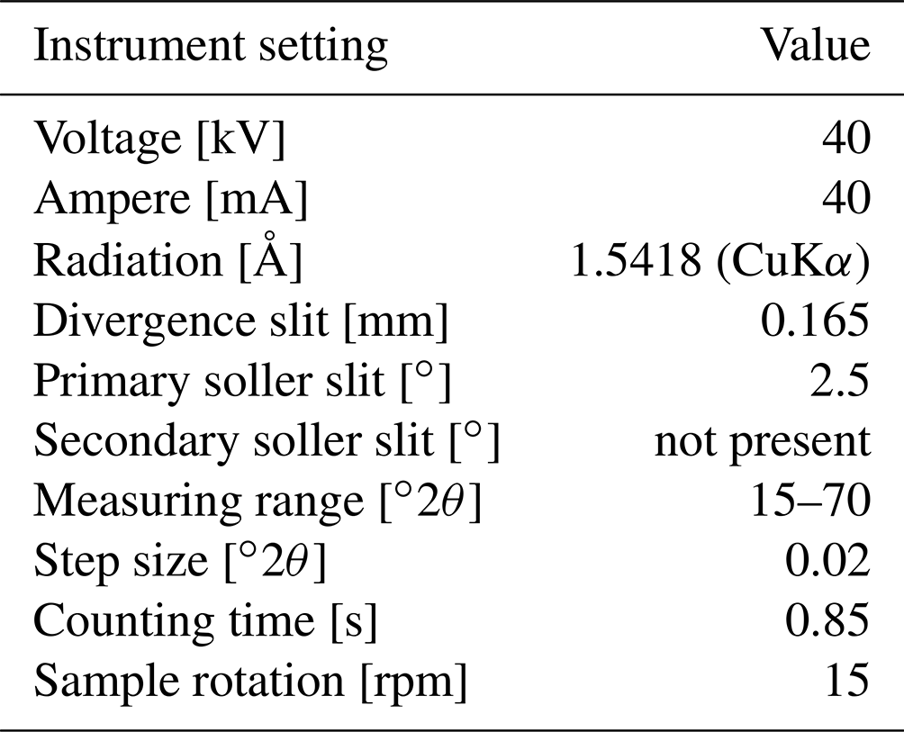
Table B1Position of each sample taken from specimens SG-126 and SG-127, measured from the umbo to the centre line of the shell (along the axis of maximum growth).
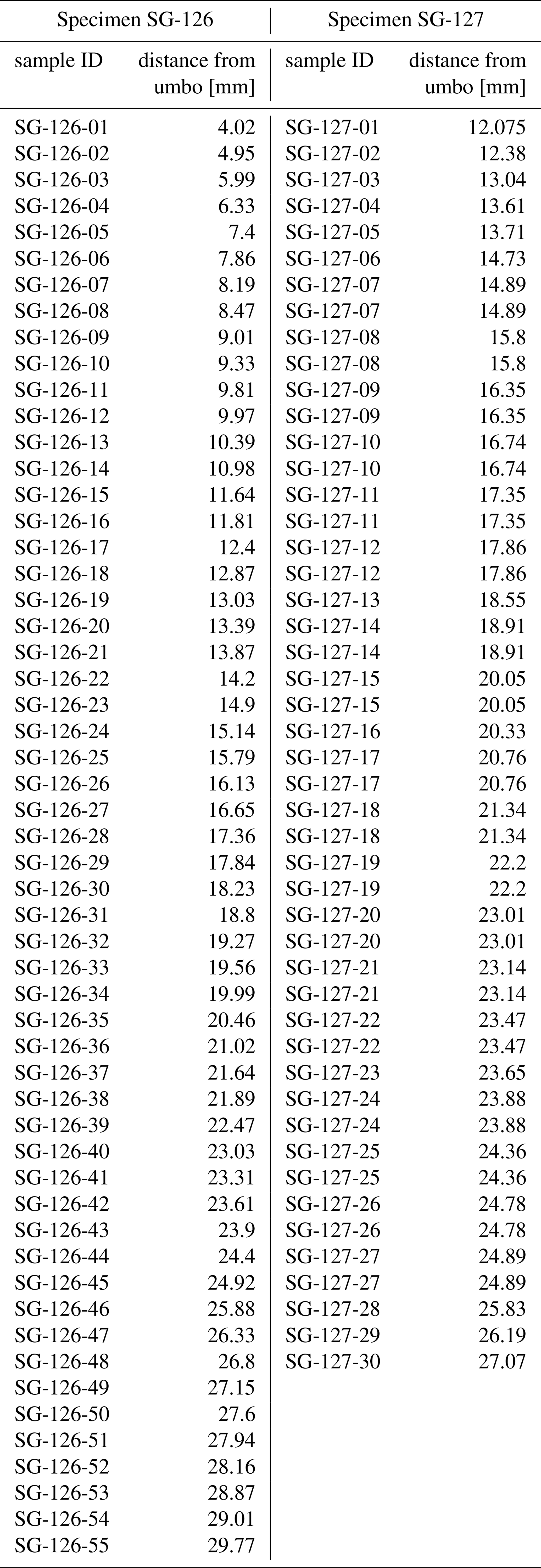
Table B2Accepted values for stable isotope standards, both oxygen and clumped.
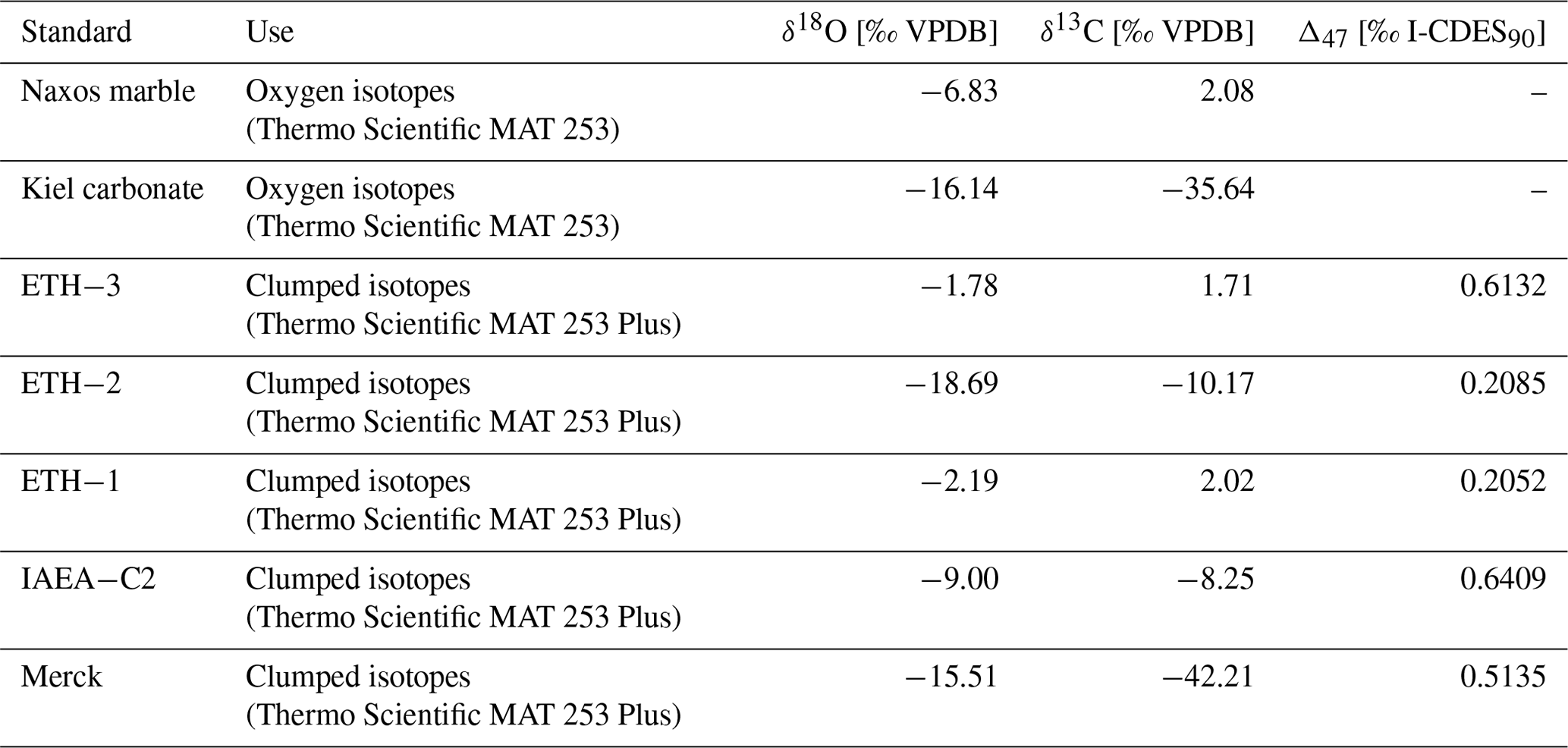
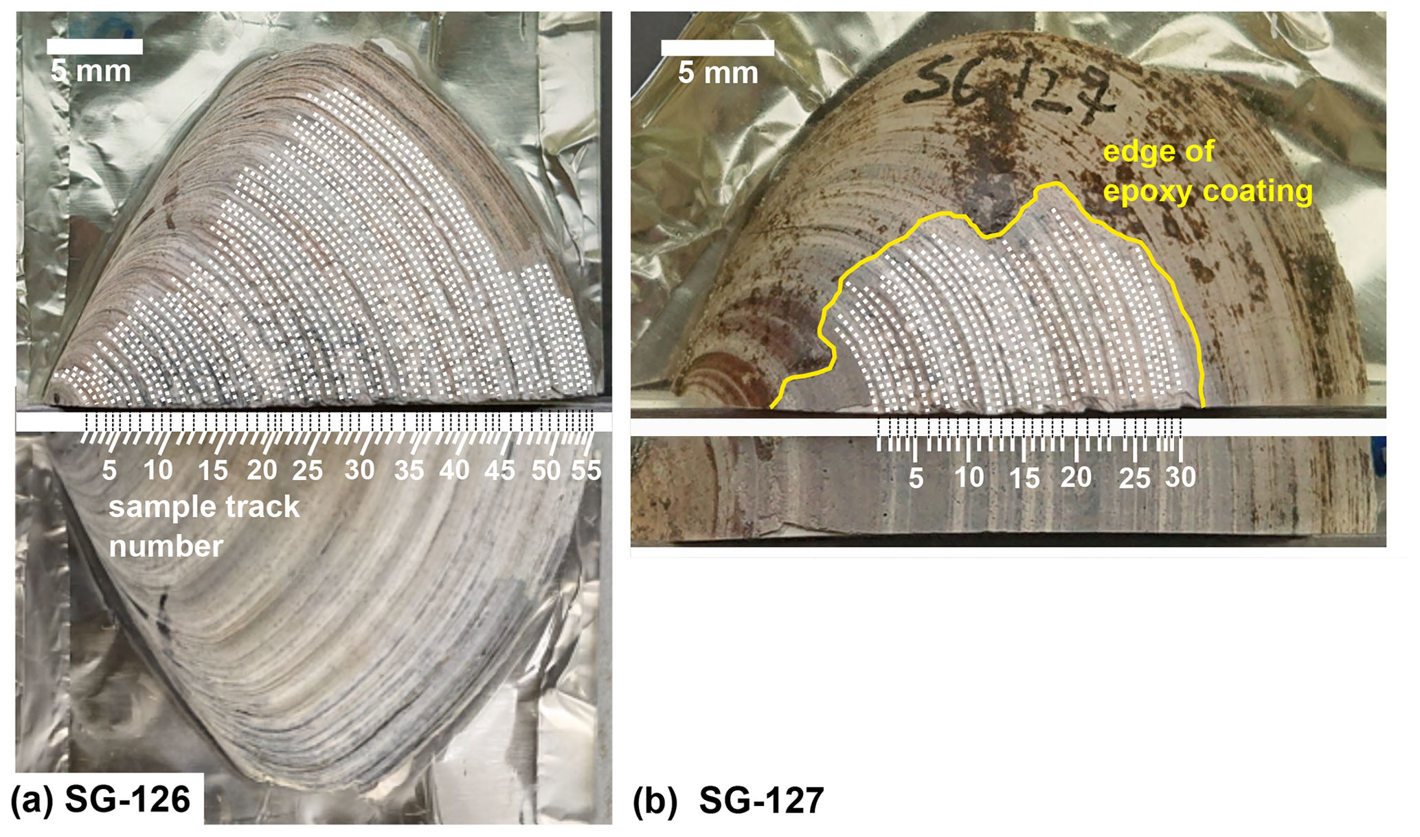
Figure B1Sampling procedure of the shells for stable isotope analysis. (a) Sample tracks on specimen SG-126, indicated by dotted lines; 55 in total, each fifth sample track has been labelled. The figure shows the sampled half (top) and that same half prior to sampling (bottom). (b) Sample tracks on specimen SG-127, indicated by dotted lines, 30 in total. This specimen was for the large part covered by epoxy, so only a small section at the upper surface could be sampled.
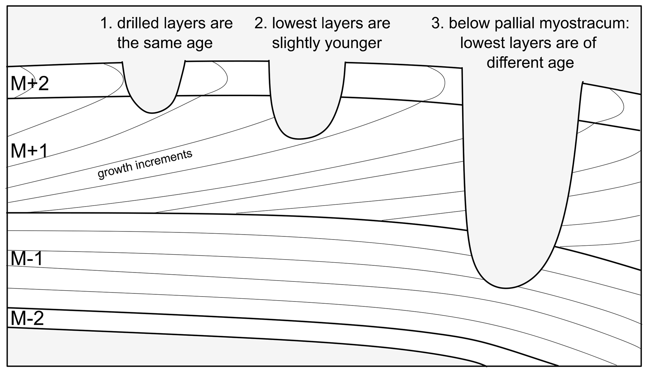
Figure B2Illustration of the importance of not drilling too deep. In scenario 1, the two outermost layers (M+2, M+1) are drilled, whose material was precipitated at the same time. In scenario 2, slightly younger material from M+1 is drilled as well. In scenario 3, material from below the pallial myostracum which separates M+1 and M−1 is drilled. As a result of the way bivalves grow, this results in mixing materials of very different precipitation ages. In addition, in this scenario materials are precipitated from different internal fluids (dorsal and ventral of the pallial line). In this study, scenario 1 was the goal. Some sampling according to scenario 2 may have been present, but scenario 3 was avoided.
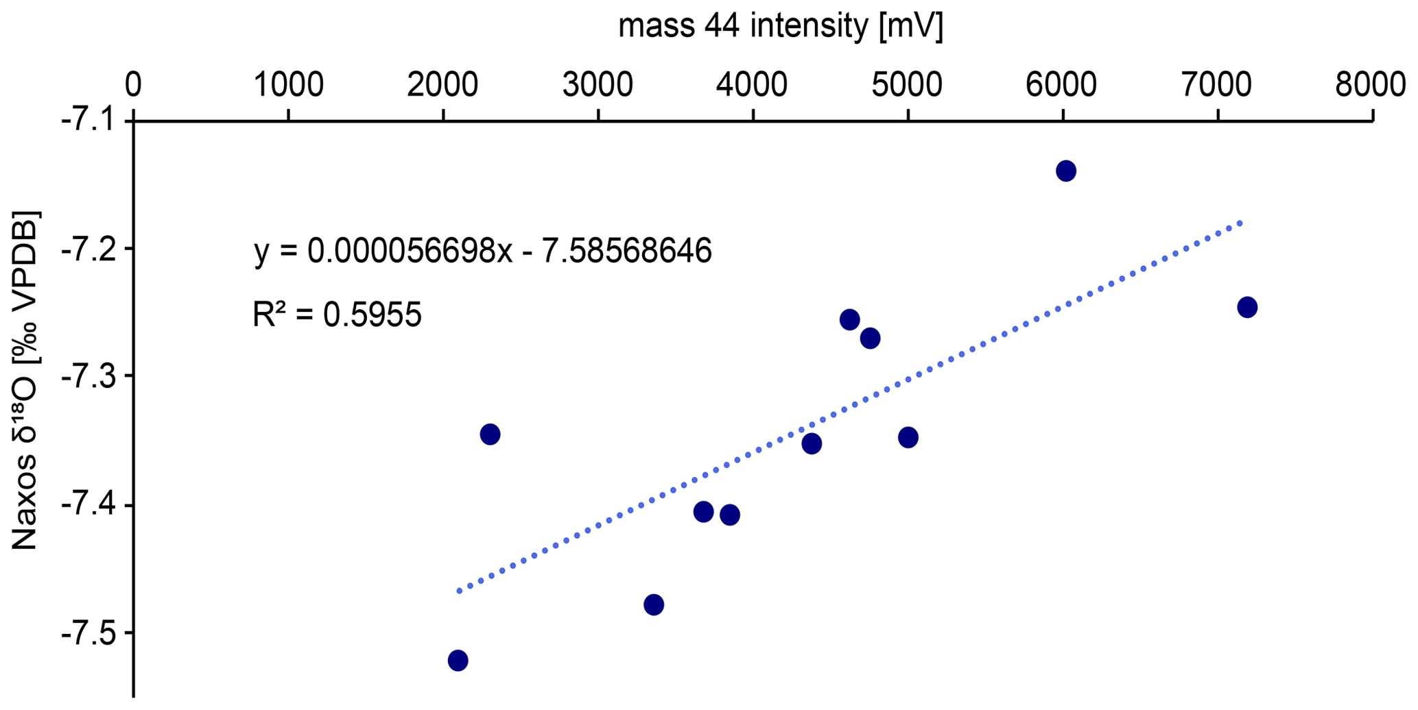
Figure B3Linear correlation between the Naxos δ18O data (11 standards measured) and the mass 44 intensity that was used to correct the δ18O data. The correction was required due to the recommended weight range for each aliquot as per the laboratory’s protocol it was quite large (50–100 µg). This results in a broad range of mass 44 values as well.
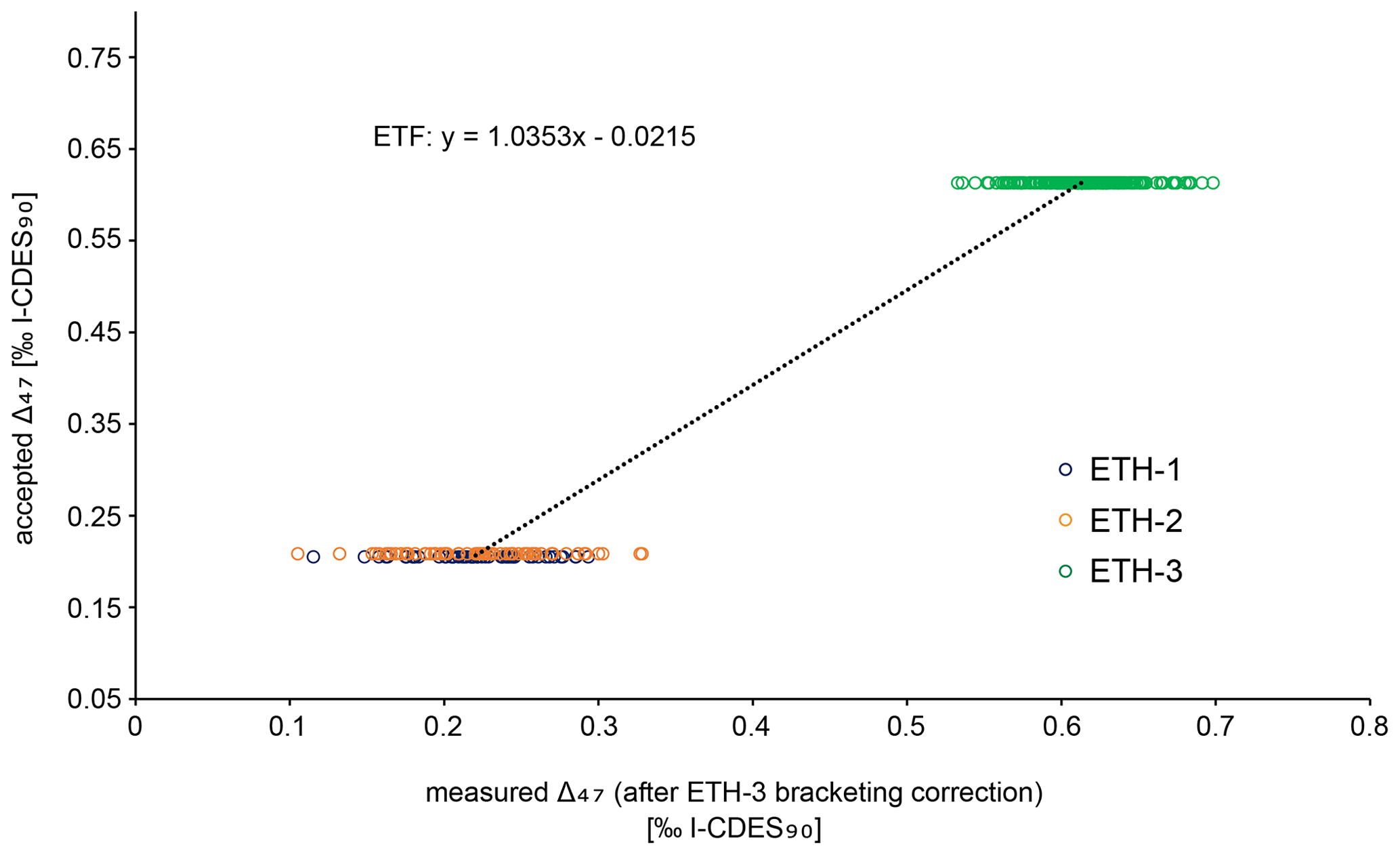
Figure B4Empirical transfer function (ETF) constructed from a linear regression between accepted and measured Δ47 values from standards ETH-1, ETH-2, and ETH-3. This function was used to correct all samples and standards and transfer them to the I-CDES90C reference frame. All standards plotted here have already been corrected for potential drift during the measurement by the ETH-3 bracketing correction. The standards were measured during 28 runs over a period of 2 months.
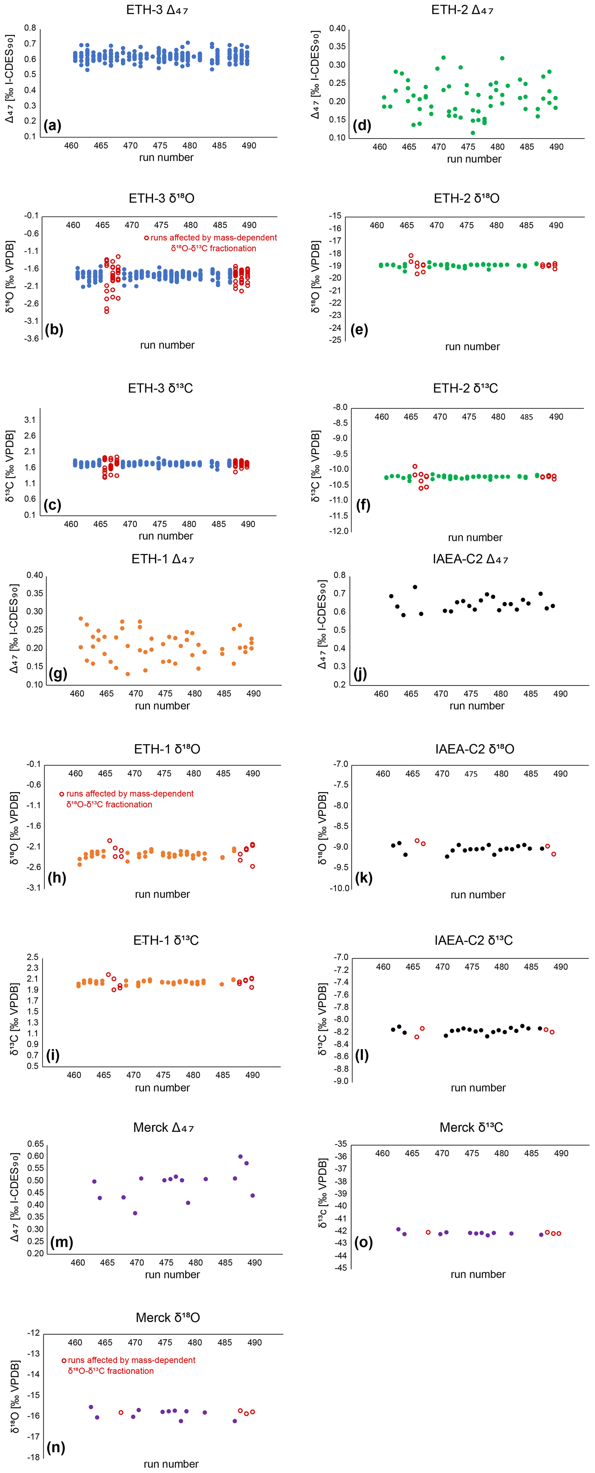
Figure B5Corrected Δ47 data for external (ETH-3, ETH-2, ETH-1) and internal (IAEA-C2, Merck) standards. (a)–(c): ETH-3 Δ47, 720 δ18O, and δ13O data. Each point represents the measurement of a single aliquot. (d)–(f): ETH-2 Δ47, δ18O, and δ13O data. (g)–(i): ETH-1 Δ47, δ18O, and δ13O data. (j)–(l): IAEA-C2 Δ47, δ18O, and δ13O data. (m)–(o): Merck Δ47, δ18O, and δ13O data. δ18O and δ13O measurements affected by mass-dependent fractionation are marked as red open circles (see Sect. 3.5.3).
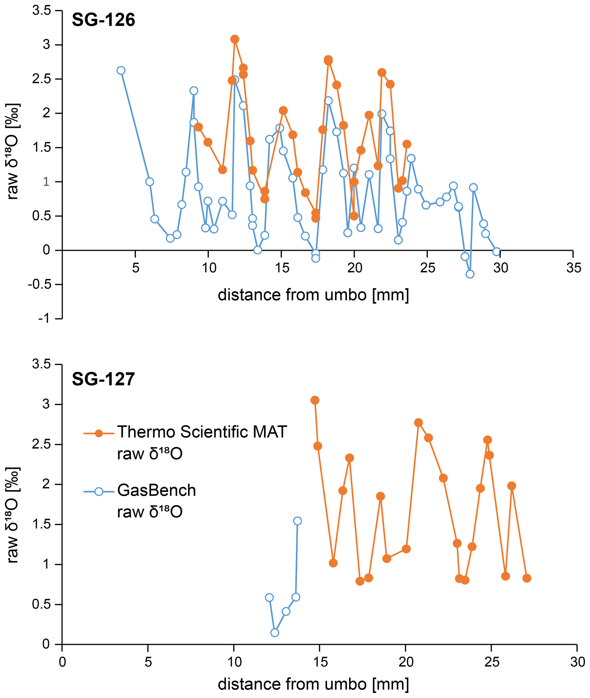
Figure B6Raw δ18Oc data for specimens SG-126 (top) and SG-127 (bottom), measured on the two different instruments as detailed in Sect. 3.5.2 and 3.5.3. The raw GasBench data shown here are not corrected for mass 44 variability yet (see Fig. B3), which explains the offset between the two records. All analyses described in the main text and subsequent plots concern the corrected GasBench data.
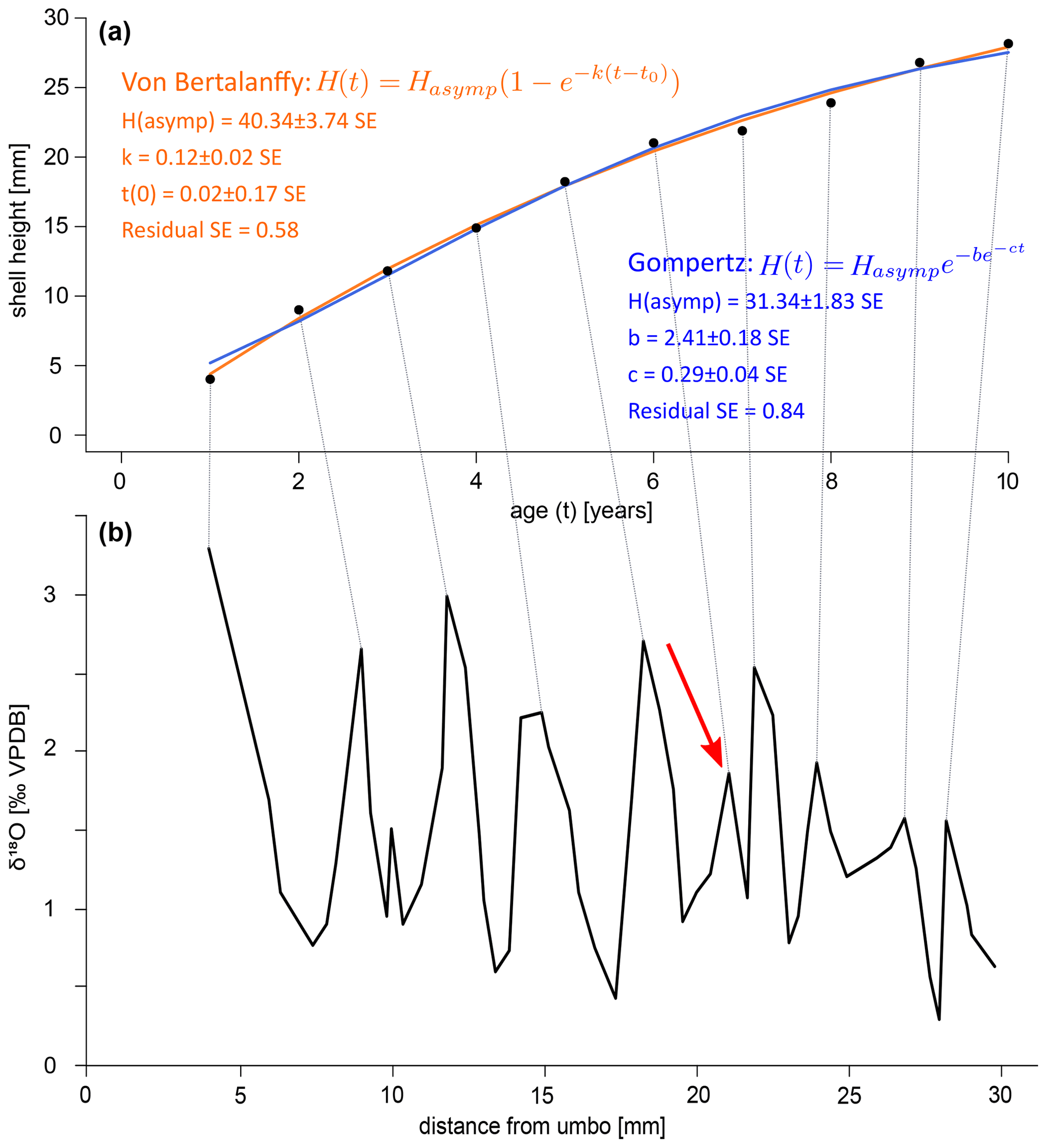
Figure B7Alternative growth curves for specimen SG-126, counting the peak at 21 mm as a year (marked with red arrow in panel b). (a) Growth curves constructed by inserting the counted years versus distance-from-umbo data points into two different fitting algorithms: the asymptotic Von Bertalanffy growth function and the logistic Gompertz function. Compared to the growth curves that do not include this peak at 21 mm, the residuals are slightly worse for both models (0.51 vs. 0.58 for the Von Bertalanffy model, 0.63 vs. 0.84 for the Gompertz model). The estimated maximum shell height is similar for the Gompertz model (34.11 vs. 31.34 mm), but significantly shorter for the Von Bertalanffy model (52.35 vs. 40.34 mm). (b) δ18Oc record with the inferred growth years marked by lines connecting to plot (a).
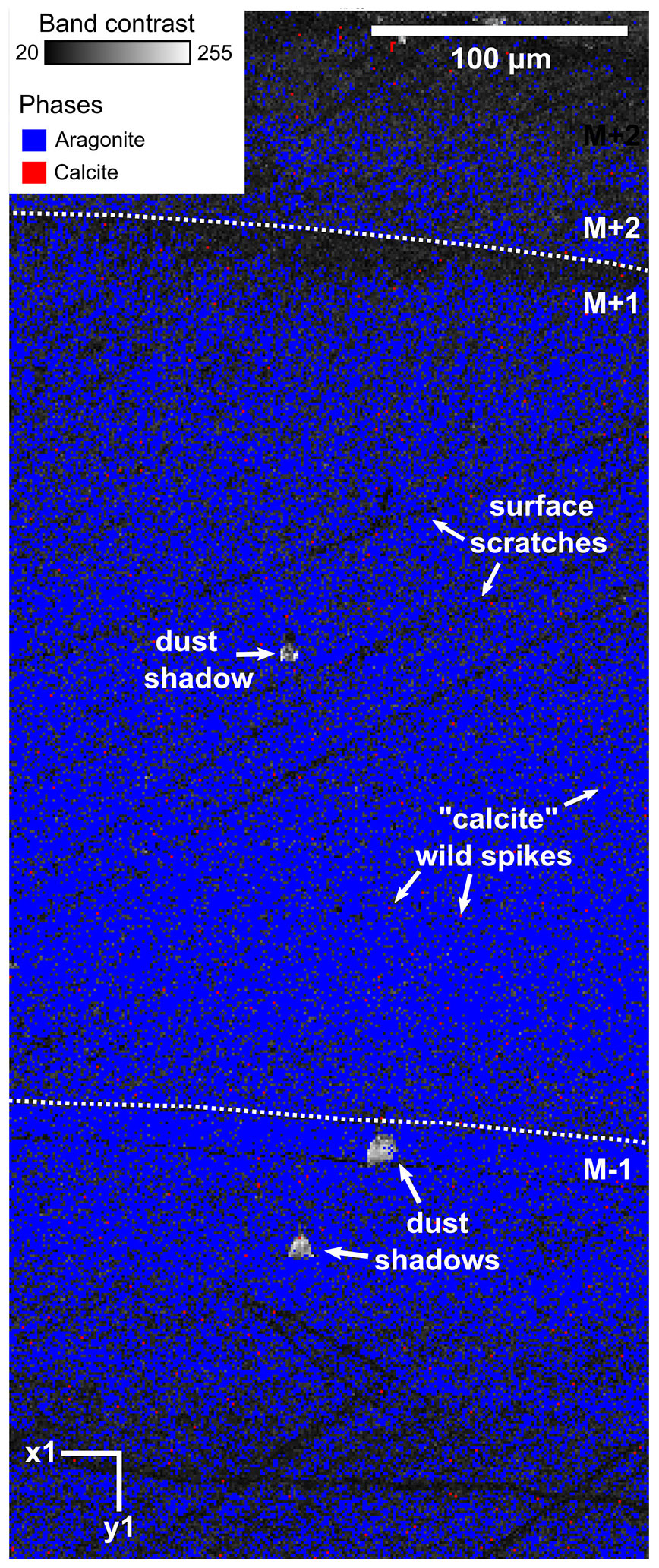
Figure C1EBSD map of specimen SG-125 indicating the absence secondary calcite crystals. Map acquisition specifics: 10 kV voltage, 1 µm step size. Measured at low vacuum due to excessive charging. Classification: 54.6 % aragonite, 45.2 % unclassified, 0.2 % calcite. The map consists of the band contrast overlain by the classified pixels, which are either aragonite (blue) or calcite (red). M+2, M+1, and M−1 correspond to the shell layers as described in Sect. 4.1.1. No clean-up was done on this map. The pixels identified as calcite do not show any of the characteristics of actual secondary calcite (large crystals compared to the fine-grained aragonite, breaking up the aragonitic structure), are always single pixels, and are removed through AZtecCrystal's wild spike removal algorithm. Several dust shadows are also seen in this image; these areas are unclassified. There are also several scratches present on the surface.
All code used was written in R. Codes for Monte Carlo error propagation (Benedeni_Monte_Carlo.R) and growth modelling (Benedeni_Growth_Model.R) are available on the GitHub repository at https://github.com/NMAWichern/Benedeni_benedeni (https://doi.org/10.5281/zenodo.8014460, Wichern, 2023).
Oxygen and carbon isotope, clumped isotope, X-ray fluorescence, X-ray diffraction, and electron backscatter diffraction data are available on the PANGAEA data repository at https://doi.org/10.1594/PANGAEA.951419 (Wichern et al., 2022).
NJdW designed the study, carried out X-ray fluorescence and X-ray diffraction measurements, and supervised in the clumped isotope lab and microscopy work. NMAW carried out stable isotope measurements, analysed all data, and wrote the original manuscript. ALAJ assisted with sclerochronology and ecological and environmental interpretations. SG provided the shell material and carried out the palaeoenvironmental interpretation of the Oorderen Formation. FW carried out the taxonomical analysis of the shells and assisted with ecological interpretation. PK and PC carried out micro-X-ray fluorescence measurements and analysis. MFH carried out electron backscatter diffraction analyses and assisted with their interpretation. MZ supervised the project and aided in data analysis. All authors contributed to interpreting the compiled data and editing the manuscript.
The contact author has declared that none of the authors has any competing interests.
Publisher’s note: Copernicus Publications remains neutral with regard to jurisdictional claims in published maps and institutional affiliations.
The authors gratefully acknowledge the following people for their help with this work: Leonard Bik (Utrecht University) made the polished thin sections for microscopy and EBSD work. Desmond Eefting and Arnold van Dijk (Utrecht University) provided technical assistance during isotope analyses. Lucas Lourens (Utrecht University) proofread the original version of this manuscript. Maarten Zeylmans (Utrecht University) helped produce high-resolution scans of cross sections of the specimens. Pim Kaskes is supported by a Research Foundation Flanders (FWO) PhD Fellowship (11E6621N). Stijn Goolaerts is grateful to Ir Murielle Reyns, Roger Sieckelink, and Nouredine Ouifak of “Mobiliteit en Openbare Werken (MOW)” for granting access to the Deurganckdoksluis construction site (2012–2014) allowing the collection of the study material. Andrew L. A. Johnson was funded by award RPG-2021-090 from the Leverhulme Trust. This work is part of the UNBIAS project funded by a Flemish Research Foundation (FWO; 12ZB220N) post-doctoral fellowship (Niels J. de Winter). The manuscript was greatly improved by the insightful comments of two anonymous reviewers, as well as Paul Butler.
This work is part of the UNBIAS project funded by a Flemish Research Foundation (FWO; grant no. 12ZB220N) post-doctoral fellowship (Niels J. de Winter). Pim Kaskes is supported by a Research Foundation Flanders (FWO) PhD Fellowship (grant no. 11E6621N). Philippe Claeys acknowledges the support of the FWO Hercules program for the purchase of the uXRF instrument and that of the VUB Strategic Research Program. Andrew L. A. Johnson was funded by award RPG-2021-090 from the Leverhulme Trust.
This paper was edited by Tina Treude and reviewed by Paul Butler and two anonymous referees.
Al-Aasm, I. S. and Veizer, J.: Diagenetic stabilization of aragonite and low-Mg calcite, I.: Trace elements in rudists, J. Sediment. Petrol., 56, 138–152, https://doi.org/10.1306/212F88A5-2B24-11D7-8648000102C1865D, 1986.
Balson, P. S., Mathers, S. J., and Zalasiewicz, J. A.: The lithostratigraphy of the Coralline Crag (Pliocene) of Suffolk, Proc. Geol. Assoc., 104, 59–70, https://doi.org/10.1016/S0016-7878(08)80155-1, 1993.
Bernasconi, S. M., Müller, I. A., Bergmann, K. D., Breitenbach, S. F. M., Fernandez, A., Hodell, D. A., Jaggi, M., Meckler, A. N., Millan, I., and Ziegler, M.: Reducing Uncertainties in Carbonate Clumped Isotope Analysis Through Consistent Carbonate-Based Standardization, Geochem. Geophy. Geosy., 19, 2895–2914, https://doi.org/10.1029/2017GC007385, 2018.
Bernasconi, S. M., Daëron, M., Bergmann, K. D., Bonifacie, M., Meckler, A. N., Affek, H. P., Anderson, N., Bajnai, D., Barkan, E., Beverly, E., Blamart, D., Burgener, L., Calmels, D., Chaduteau, C., Clog, M., Davidheiser-Kroll, B., Davies, A., Dux, F., Eiler, J., Elliott, B., Fetrow, A. C., Fiebig, J., Goldberg, S., Hermoso, M., Huntington, K. W., Hyland, E., Ingalls, M., Jaggi, M., John, C. M., Jost, A. B., Katz, S., Kelson, J., Kluge, T., Kocken, I. J., Laskar, A., Leutert, T. J., Liang, D., Lucarelli, J., Mackey, T. J., Mangenot, X., Meinicke, N., Modestou, S. E., Müller, I. A., Murray, S., Neary, A., Packard, N., Passey, B. H., Pelletier, E., Petersen, S., Piasecki, A., Schauer, A., Snell, K. E., Swart, P. K., Tripati, A., Upadhyay, D., Vennemann, T., Winkelstern, I., Yarian, D., Yoshida, N., Zhang, N., and Ziegler, M.: InterCarb: A Community Effort to Improve Interlaboratory Standardization of the Carbonate Clumped Isotope Thermometer Using Carbonate Standards, Geochem. Geophy. Geosy., 22, e2020GC009588, https://doi.org/10.1029/2020GC009588, 2021.
Bieler, R., Mikkelsen, P. M., Collins, T. M., Glover, E. A., González, V. L., Graf, D. L., Harper, E. M., Healy, J., Kawauchi, G. Y., Sharma, P. P., Staubach, S., Strong, E. E., Taylor, J. D., Tëmkin, I., Zardus, J. D., Clark, S., Guzmán, A., McIntyre, E., Sharp, P., and Giribet, G.: Investigating the Bivalve Tree of Life – an exemplar-based approach combining molecular and novel morphological characters, Invert. Systematics, 28, 32–115, https://doi.org/10.1071/IS13010, 2014.
Brand, U. and Veizer, J.: Chemical Diagenesis of a Multicomponent Carbonate System; 1: Trace Elements, J. Sediment. Res., 50, 1219–1236, https://doi.org/10.1306/212F7BB7-2B24-11D7-8648000102C1865D, 1980.
Brand, W. A., Assonov, S. S., and Coplen, T. B.: Correction for the 17O interference in δ(13C) measurements when analyzing CO2 with stable isotope mass spectrometry (IUPAC Technical Report), Pure Appl. Chem., 82, 1719–1733, https://doi.org/10.1351/PAC-REP-09-01-05, 2010.
Butler, P. G., Wanamaker Jr., A. D., Scourse, J. D., Richardson, C. A., and Reynolds, D. J.: Variability of marine climate on the North Icelandic Shelf in a 1357-year proxy archive based on growth increments in the bivalve Arctica islandica, Palaeogeogr. Palaeocl., 373, 141–151, https://doi.org/10.1016/j.palaeo.2012.01.016, 2013.
Carré, M., Bentaleb, I., Blamart, D., Ogle, N., Cardenas, F., Zevallos, S., Kalin, R. M., Ortlieb, L., and Fontugne, M.: Stable isotopes and sclerochronology of the bivalve Mesodesma donacium: potential application to Peruvian paleoceanographic reconstructions, Palaeogeogr. Palaeocl., 228, 4–25, https://doi.org/10.1016/j.palaeo.2005.03.045, 2005.
Casella, L. A., Griesshaber, E., Yin, X., Ziegler, A., Mavromatis, V., Müller, D., Ritter, A.-C., Hippler, D., Harper, E. M., Dietzel, M., Immenhauser, A., Schöne, B. R., Angiolini, L., and Schmahl, W. W.: Experimental diagenesis: insights into aragonite to calcite transformation of Arctica islandica shells by hydrothermal treatment, Biogeosciences, 14, 1461–1492, https://doi.org/10.5194/bg-14-1461-2017, 2017.
Chauvaud, L., Lorrain, A., Dunbar, R. B., Paulet, Y.-M., Thouzeau, G., Jean, F., Guarini, J.-M., and Mucciarone, D.: Shell of the Great Scallop Pecten maximus as a high-frequency archive of paleoenvironmental changes, Geochem. Geophy. Geosy., 6, Q08001, https://doi.org/10.1029/2004GC000890, 2005.
Checa, A. G., Harper, E. M., and González-Segura, A.: Structure and crystallography of foliated and chalk shell microstructures of the oyster Magallana: the same materials grown under different conditions, Sci. Rep., 8, 7507, https://doi.org/10.1038/s41598-018-25923-6, 2018.
Cochran, J. K., Kallenberg, K., Landman, N. H., Harries, P. J., Weinreb, D., Turekian, K. K., Beck, A. J., and Cobban, W. A.: Effect of diagenesis on the Sr, O, and C isotope composition of late Cretaceous mollusks from the Western Interior Seaway of North America, Am. J. Sci., 310, 69–88, https://doi.org/10.2475/02.2010.01, 2010.
Crippa, G., Griesshaber, E., Checa, A. G., Harper, E. M., Simonet Roda, M., and Schmahl, W. W.: Orientation patterns of aragonitic crossed-lamellar, fibrous prismatic and myostracal microstructures of modern Glycymeris shells, J. Struct. Biol., 212, 107653, https://doi.org/10.1016/j.jsb.2020.107653, 2020.
Cusack, M.: Biomineral electron backscatter diffraction for palaeontology, Palaeontology, 59, 171–179, https://doi.org/10.1111/pala.12222, 2016.
Deckers, J., Louwye, S., and Goolaerts, S.: The internal division of the Pliocene Lillo Formation: correlation between Cone Penetration Tests and lithostratigraphic type sections, Geol. Belgica, 23, 333–343, https://doi.org/10.20341/gb.2020.027, 2020.
De Meuter, F. J. and Laga, P. G.: Lithostratigraphy and biostratigraphy based on benthonic foraminifera of the Neogene deposits of northern Belgium, Bulletin van de Belgische Vereniging voor Geologie, 85, 133–152, 1976.
De Schepper, S., Head, M. J., and Louwye, S.: Pliocene dinoflagellate cyst stratigraphy, palaeoecology and sequence stratigraphy of the Tunnel-Canal Dock, Belgium, Geol. Mag., 146, 92–112, https://doi.org/10.1017/S0016756808005438, 2009.
Dettman, D. L., Reische, A. K., and Lohmann, K. C.: Controls on the stable isotope composition of seasonal growth bands in aragonitic fresh-water bivalves (unionidae), Geochim. Cosmochim. Ac., 63, 1049–1057, https://doi.org/10.1016/S0016-7037(99)00020-4, 1999.
de Winter, N. J. and Claeys, P.: Micro X-ray fluorescence (μXRF) line scanning on Cretaceous rudist bivalves: A new method for reproducible trace element profiles in bivalve calcite, Sedimentology, 64, 231–251, https://doi.org/10.1111/sed.12299, 2017.
de Winter, N. J., Sinnesael, M., Makarona, C., Vansteenberge, S., and Claeys, P.: Trace element analyses of carbonates using portable and micro-X-ray fluorescence: performance and optimization of measurement parameters and strategies, J. Anal. At. Spectrom., 32, 1211–1223, https://doi.org/10.1039/C6JA00361C, 2017a.
de Winter, N. J., Goderis, S., Dehairs, F., Jagt, J. W. M., Fraaije, R. H. B., van Malderen, S. J. M., Vanhaecke, F., and Claeys, P.: Tropical seasonality in the late Campanian (late Cretaceous): Comparison between multiproxy records from three bivalve taxa from Oman, Palaeogeogr. Palaeocl., 485, 740–760, https://doi.org/10.1016/j.palaeo.2017.07.031, 2017b.
de Winter, N. J., Vellekoop, J., Clark, A. J., Stassen, P., Speijer, R. P., and Claeys, P.: The Giant Marine Gastropod Campanile Giganteum (Lamarck, 1804) as a High-Resolution Archive of Seasonality in the Eocene Greenhouse World, Geochem. Geophy. Geosy., 21, e2019GC008794, https://doi.org/10.1029/2019GC008794, 2020.
de Winter, N. J., Agterhuis, T., and Ziegler, M.: Optimizing sampling strategies in high-resolution paleoclimate records, Clim. Past, 17, 1315–1340, https://doi.org/10.5194/cp-17-1315-2021, 2021a.
de Winter, N. J., Dämmer, L. K., Falkenroth, M., Reichart, G.-J., Moretti, S., Martínez-García, A., Höche, N., Schöne, B. R., Rodiouchkina, K., Goderis, S., Vanhaecke, F., van Leeuwen, S. M., and Ziegler, M.: Multi-isotopic and trace element evidence against different formation pathways for oyster microstructures, Geochim. Cosmochim. Ac., 308, 326–352, https://doi.org/10.1016/j.gca.2021.06.012, 2021b.
de Winter, N. J., Witbaard, R., Kocken, I. J., Müller, I. A., Guo, J., Goudsmit, B., and Ziegler, M.: Temperature Dependence of Clumped Isotopes (Δ47) in Aragonite, Geophys. Res. Lett., 49, e2022GL099479, https://doi.org/10.1029/2022GL099479, 2022.
Dowsett, H. J., Robinson, M., Haywood, A. M., Salzmann, U., Hill, D. J., Sohl, L., Chandler, M. A., Williams, M., Foley, K., and Stoll, D.: The PRISM3D paleoenvironmental reconstruction, Stratigraphy, 7, 123–139, 2010.
Dowsett, H. J., Robinson, M. M., Haywood, A. M., Hill, D. J., Dolan, A. M., Stoll, D. K., Chan, W.-L., Abe-Ouchi, A., Chandler, M. A., Rosenbloom, N. A., Otto-Bliesner, B. L., Bragg, F. J., Lunt, D. J., Foley, K. M., and Riesselman, C. R.: Assessing confidence in Pliocene sea surface temperatures to evaluate predictive models, Nat. Clim. Change, 2, 365–371, https://doi.org/10.1038/NCLIMATE1455, 2012.
Dowsett, H. J., Foley, K. M., Stoll, D. K., Chandler, M. A., Sohl, L. E., Bentsen, M., Otto-Bliesner, B. L., Bragg, F. J., Chan, W.-L., Contoux, C., Dolan, A. M., Haywood, A. M., Jonas, J. A., Jost, A., Kamae, Y., Lohmann, G., Lunt, D. J., Nisancioglu, K. H., Abe-Ouchi, A., Ramstein, G., Riesselman, C. R., Robinson, M. M., Rosenbloom, N. A., Salzmann, U., Stepanek, C., Strother, S. L., Ueda, H., Yan, Q., and Zhang, Z.: Sea surface temperature of the mid-Piacenzian ocean: a data-model comparison, Sci. Rep., 3, 2013, https://doi.org/10.1038/srep02013, 2013.
Dowsett, H. J., Dolan, A. M., Rowley, D., Moucha, R., Forte, A. M., Mitrovica, J. X., Pound, M., Salzmann, U., Robinson, M., Chandler, M. A., Foley, K., and Haywood, A. M.: The PRISM4 (mid-Piacenzian) paleoenvironmental reconstruction, Clim. Past, 12, 1519–1538, https://doi.org/10.5194/cp-12-1519-2016, 2016.
Emeis, K.-C., van Beusekom, J., Callies, U., Ebinghaus, R., Kannen, A., Kraus, G., Kröncke, I., Lenhart, H., Lorkowski, I., Matthias, V., Möllmann, C., Pätsch, J., Scharfe, M., Thomas, H., Weisse, R., and Zorita, E.: The North Sea – A shelf sea in the Anthropocene, J. Mar. Syst., 141, 18–33, https://doi.org/10.1016/j.jmarsys.2014.03.012, 2015.
Gaemers, P. A. M.: Enkele paleo-ecologische opmerkingen over de Pliocene afzettingen in de tunnelput nabij Kallo, België, provincie Oost Vlaanderen, deel 2, Mededelingen van de Werkgroep voor Tertiaire en Kwartaire Geologie, 12, 43–49, 1975.
Ghosh, P., Adkins, J., Affek, H. P., Balta, B., Guo, W., Schauble, E. A., Schrag, D. P., and Eiler, J. M.: 13C–18O bonds in carbonate minerals: A new kind of paleothermometer, Geochim. Cosmochim. Ac., 70, 1439–1456, https://doi.org/10.1016/j.gca.2005.11.014, 2006.
Gibbard, P. L. and Lewin, J.: Filling the North Sea Basin: Cenozoic sediment sources and river styles (André Dumont medallist lecture 2014), Geol. Belgica, 19, 201–217, https://doi.org/10.20341/gb.2015.017, 2016.
Griesshaber, E., Schmahl, W. W., Ubhi, H. S., Huber, J., Nindiyasari, F., Maier, B., and Ziegler, A.: Homoepitaxial meso- and microscale crystal co-orientation and organic matrix network structure in Mytilus edulis nacre and calcite, Acta Biomater., 9, 9492–9502, https://doi.org/10.1016/j.actbio.2013.07.020, 2013.
Grossman, E. L. and Ku, T.-L.: Oxygen and carbon isotope fractionation in biogenic aragonite: temperature effects, Chem. Geol., 59, 59–74, https://doi.org/10.1016/0168-9622(86)90057-6, 1986.
Harwood, A. J. P., Dennis, P. F., Marca, A. D., Pilling, G. M., and Millner, R. S.: The oxygen isotope composition of water masses within the North Sea, Estuar. Coast. Shelf Sci., 78, 353–359, https://doi.org/10.1016/j.ecss.2007.12.010, 2008.
Haywood, A. M. and Valdes, P. J.: Modelling Pliocene warmth: contribution of atmosphere, oceans and cryosphere, Earth Planet. Sc. Lett., 218, 363–377, https://doi.org/10.1016/S0012-821X(03)00685-X, 2004.
Haywood, A. M., Tindall, J. C., Dowsett, H. J., Dolan, A. M., Foley, K. M., Hunter, S. J., Hill, D. J., Chan, W.-L., Abe-Ouchi, A., Stepanek, C., Lohmann, G., Chandan, D., Peltier, W. R., Tan, N., Contoux, C., Ramstein, G., Li, X., Zhang, Z., Guo, C., Nisancioglu, K. H., Zhang, Q., Li, Q., Kamae, Y., Chandler, M. A., Sohl, L. E., Otto-Bliesner, B. L., Feng, R., Brady, E. C., von der Heydt, A. S., Baatsen, M. L. J., and Lunt, D. J.: The Pliocene Model Intercomparison Project Phase 2: large-scale climate features and climate sensitivity, Clim. Past, 16, 2095–2123, https://doi.org/10.5194/cp-16-2095-2020, 2020.
He, B., Olack, G. A., and Colman, A. S.: Pressure baseline correction and high-precision CO2 clumped-isotope (Δ47) measurements in bellows and micro-volume modes: PBL-corrected high-precision CO2 clumped-isotope (Δ47) measurements, Rapid Commun. Mass Sp., 26, 2837–2853, https://doi.org/10.1002/rcm.6436, 2012.
Hendry, J. P., Ditchfield, P. W., and Marshall, J. D.: Two-Stage Neomorphism of Jurassic Aragonitic Bivalves: Implications for Early Diagenesis, J. Sediment. Res., 65, 214–224, https://doi.org/10.1306/D4268077-2B26-11D7-8648000102C1865D, 1995.
Hu, B., Radke, J., Schlüter, H.-J., Torsten Heine, F., Zhou, L., and Bernasconi, S. M.: A modified procedure for gas-source isotope ratio mass spectrometry: The long-integration dual-inlet (LIDI) methodology and implications for clumped isotope measurements, Rapid Commun. Mass Sp., 28, 1413–1425, https://doi.org/10.1002/rcm.6909, 2014.
Huyghe, D., Daëron, M., de Rafelis, M., Blamart, D., Sébilo, M., Paulet, Y.-M., and Lartaud, F.: Clumped isotopes in modern marine bivalves, Geochim. Cosmochim. Ac., 316, 41–58, https://doi.org/10.1016/j.gca.2021.09.019, 2022.
IPCC: Summary for Policymakers, in: Climate Change 2021: The Physical Science Basis, Contribution of Working Group I to the Sixth Assessment Report of the Intergovernmental Panel on Climate Change, edited by: Masson-Delmotte, V., Zhai, P., Pirani, A., Connors, S. L., Péan, C., Berger, S., Caud, N., Chen, Y., Goldfarb, L., Gomis, M. I., Huang, M., Leitzell, K., Lonnoy, E., Matthews, J. B. R., Maycock, T. K., Waterfield, T., Yelekçi, O., Yu, R., and Zhou, B., Cambridge University Press, Cambridge, United Kingdom and New York, NY, USA, 3–32, https://doi.org/10.1017/9781009157896.001, 2021.
Johnson, A. L. A., Hickson, J. A., Bird, A., Schöne, B. R., Balson, P. S., Heaton, T. H. E., and Williams, M.: Comparative sclerochronology of modern and mid-Pliocene (c. 3.5 Ma) Aequipecten opercularis (Mollusca, Bivalvia): an insight into past and future climate change in the north-east Atlantic region, Palaeogeogr. Palaeocl., 284, 164–179, https://doi.org/10.1016/j.palaeo.2009.09.022, 2009.
Johnson, A. L. A., Valentine, A. M., Schöne, B. R., Leng, M. J., and Goolaerts, S.: Sclerochronological evidence of pronounced seasonality from the late Pliocene of the southern North Sea basin and its implications, Clim. Past, 18, 1203–1229, https://doi.org/10.5194/cp-18-1203-2022, 2022.
Jones, D. S., Quitmyer, I. R., and Andrus, C. F. T.: Oxygen isotopic evidence for greater seasonality in Holocene shells of Donax variabilis from Florida, Palaeogeogr. Palaeocl., 228, 96–108, https://doi.org/10.1016/j.palaeo.2005.03.046, 2005.
Judd, E. J., Wilkinson, B. H., and Ivany, L. C.: The life and time of clams: Derivation of intra-annual growth rates from high-resolution oxygen isotope profiles, Palaeogeogr. Palaeocl., 490, 70–83, https://doi.org/10.1016/j.palaeo.2017.09.034, 2018.
Kaskes, P., Déhais, T., de Graaff, S. J., Goderis, S., and Claeys, P.: Micro–X-ray fluorescence (μXRF) analysis of proximal impactites: High-resolution element mapping, digital image analysis, and quantifications, in: Large Meteorite Impacts and Planetary Evolution VI, edited by: Reimold, W. U. and Koeberl, C., Geological Society of America Special Paper 550, 171–206, https://doi.org/10.1130/2021.2550(07), 2021.
Kobayashi, I. and Akai, J.: Twinned aragonite crystals found in the bivalvian crossed lamellar shell structure, J. Geol. Soc. Jpn., 100, 177–180, https://doi.org/10.5575/geosoc.100.177, 1994.
Kocken, I. J., Müller, I. A., and Ziegler, M.: Optimizing the Use of Carbonate Standards to Minimize Uncertainties in Clumped Isotope Data, Geochem. Geophy. Geosy., 20, 5565–5577, https://doi.org/10.1029/2019GC008545, 2019.
Kooij, J., Engelhard, G. H., and Righton, D. A.: Climate change and squid range expansion in the North Sea, J. Biogeogr., 43, 2285–2298, https://doi.org/10.1111/jbi.12847, 2016.
Kvale, E. P.: The origin of neap–spring tidal cycles, Mar. Geol., 235, 5–18, https://doi.org/10.1016/j.margeo.2006.10.001, 2006.
Lafuente, B., Downs, R. T., Yang, H., and Stone, N.: The power of databases: The RRUFF project, in: Highlights in Mineralogical Crystallography, edited by: Armbruster, T. and Danisi, R. M., De Gruyter, Berlin, München, Boston, De Gruyter, 2016, 1–30, https://doi.org/10.1515/9783110417104-003, 2015.
Lee, L., Atkinson, D., Hirst, A. G., and Cornell, S. J.: A new framework for growth curve fitting based on the von Bertalanffy Growth Function, Sci. Rep., 10, 7953, https://doi.org/10.1038/s41598-020-64839-y, 2020.
Louwye, S. and De Schepper, S.: The Miocene–Pliocene hiatus in the southern North Sea Basin (northern Belgium) revealed by dinoflagellate cysts, Geol. Mag., 147, 760–776, https://doi.org/10.1017/S0016756810000191, 2010.
Louwye, S., Head, M. J., and De Schepper, S.: Dinoflagellate cyst stratigraphy and palaeoecology of the Pliocene in northern Belgium, southern North Sea Basin, Geol. Mag., 141, 353–378, https://doi.org/10.1017/S0016756804009136, 2004.
Lutz, R. A. and Rhoads, D. C.: Growth patterns within the molluscan shell. An overview, in: Skeletal Growth of Aquatic Organisms., Plenum Press, New York, 203–254, ISBN: 0-306-40259-9. 1980.
Mackenzie, B. R. and Schiedek, D.: Daily ocean monitoring since the 1860s shows record warming of northern European seas, Glob. Change Biol., 13, 1335–1347, https://doi.org/10.1111/j.1365-2486.2007.01360.x, 2007.
Marcano, M. C., Frank, T. D., Mukasa, S. B., Lohmann, K. C., and Taviani, M.: Diagenetic incorporation of Sr into aragonitic bivalve shells: Implications for chronostratigraphic and palaeoenvironmental interpretations, Depos. Record, 1, 38–52, https://doi.org/10.1002/dep2.3, 2015.
Marquet, R. T. C.: Ecology and evolution of Pliocene bivalves from the Antwerp Basin, Bulletin de l'Institut royal des Sciences naturelles de Belgique, Sciences de la terre, 74, 205–212, 2004.
Marquet, R. T. C.: The Neogene Bivalvia (Heterodonta and Anomalodesmata) and Scaphopoda from Kallo and Doel (Oost-Vlaanderen, Belgium), Palaeontos, 6, 1–142, 2005.
McConnaughey, T. A. and Gillikin, D. P.: Carbon isotopes in mollusk shell carbonates, Geo-Mar. Lett., 28, 287–299, https://doi.org/10.1007/s00367-008-0116-4, 2008.
Meckler, A. N., Ziegler, M., Millán, M. I., Breitenbach, S. F. M., and Bernasconi, S. M.: Long-term performance of the Kiel carbonate device with a new correction scheme for clumped isotope measurements: Performance and correction of Kiel clumped isotope measurements, Rapid Commun. Mass Sp., 28, 1705–1715, https://doi.org/10.1002/rcm.6949, 2014.
Meinicke, N., Ho, S. L., Hannisdal, B., Nürnberg, D., Tripati, A., Schiebel, R., and Meckler, A. N.: A robust calibration of the clumped isotopes to temperature relationship for foraminifers, Geochim. Cosmochim. Ac., 270, 160–183, https://doi.org/10.1016/j.gca.2019.11.022, 2020.
Meinicke, N., Reimi, M. A., Ravelo, A. C., and Meckler, A. N.: Coupled Mg Ca and Clumped Isotope Measurements Indicate Lack of Substantial Mixed Layer Cooling in the Western Pacific Warm Pool During the Last ∼ 5 Million Years, Paleoceanogr. Paleocl., 36, e2020PA004115, https://doi.org/10.1029/2020PA004115, 2021.
Milano, S., Schöne, B. R., and Witbaard, R.: Changes of shell microstructural characteristics of Cerastoderma edule (Bivalvia) – A novel proxy for water temperature, Palaeogeogr. Palaeocl., 465, 395–406, https://doi.org/10.1016/j.palaeo.2015.09.051, 2017.
Monastersky, R.: Global carbon dioxide levels near worrisome milestone, Nature, 497, 13–14, https://doi.org/10.1038/497013a, 2013.
Moon, L. R., Judd, E. J., Thomas, J., and Ivany, L. C.: Out of the oven and into the fire: Unexpected preservation of the seasonal δ18O cycle following heating experiments on shell carbonate, Palaeogeogr. Palaeocl., 562, 110115, https://doi.org/10.1016/j.palaeo.2020.110115, 2021.
Müller, I. A., Fernandez, A., Radke, J., van Dijk, J., Bowen, D., Schwieters, J., and Bernasconi, S. M.: Carbonate clumped isotope analyses with the long-integration dual-inlet (LIDI) workflow: scratching at the lower sample weight boundaries, Rapid Commun. Mass Sp., 31, 1057–1066, https://doi.org/10.1002/rcm.7878, 2017.
Nyst, P. H. and Westendorp, G. D.: Nouvelles recherches sur les coquilles fossiles de la province d'Anvers, Bulletins de l'Académie royale des Sciences et Belles-Lettres de Bruxelles, 6, 393–414, 1839.
Pagani, M., Liu, Z., LaRiviere, J., and Ravelo, A. C.: High Earth-system climate sensitivity determined from Pliocene carbon dioxide concentrations, Nat. Geosci., 3, 27–30, https://doi.org/10.1038/NGEO724, 2010.
Pannella, G. and MacClintock, C.: Biological and environmental rhythms reflected in molluscan shell growth, Memoir, 42, 64–80, https://doi.org/10.1017/S0022336000061655, 1968.
Popov, S. V.: Composite prismatic structure in bivalve shell, Acta Palaeontol. Pol., 31, 3–26, 1986.
Popov, S. V.: Formation of Bivalve Shells and Their Microstructure, Paleontol. J., 48, 1519–1531, https://doi.org/10.1134/S003103011414010X, 2014.
Preibisch, S., Saalfeld, S., and Tomancak, P.: Globally optimal stitching of tiled 3D microscopic image acquisitions, Bioinformatics, 25, 1463–1465, https://doi.org/10.1093/bioinformatics/btp184, 2009.
R Core Team: R: A language and environment for statistical computing, R Foundation for Statistical Computing, Vienna, Austria, https://www.R-project.org/ (last access: 20 June 2023), 2021.
Ritter, A.-C., Mavromatis, V., Dietzel, M., Kwiecien, O., Wiethoff, F., Griesshaber, E., Casella, L. A., Schmahl, W. W., Koelen, J., Neuser, R. D., Leis, A., Buhl, D., Niedermayr, A., Breitenbach, S. F. M., Bernasconi, S. M., and Immenhauser, A.: Exploring the impact of diagenesis on (isotope) geochemical and microstructural alteration features in biogenic aragonite, Sedimentology, 64, 1354–1380, https://doi.org/10.1111/sed.12356, 2017.
Schauble, E. A., Ghosh, P., and Eiler, J. M.: Preferential formation of 13C–18O bonds in carbonate minerals, estimated using first-principles lattice dynamics, Geochim. Cosmochim. Ac., 70, 2510–2529, https://doi.org/10.1016/j.gca.2006.02.011, 2006.
Schoeppler, V., Lemanis, R., Reich, E., Pusztai, T., Gránásy, L., and Zlotnikov, I.: Crystal growth kinetics as an architectural constraint on the evolution of molluscan shells, P. Natl. Acad. Sci. USA, 116, 20388–20397, https://doi.org/10.1073/pnas.1907229116, 2019.
Schöne, B. R., Goodwin, D. H., Flessa, K. W., Dettman, D. L., and Roopnarine, P. D.: Sclerochronology and Growth of the Bivalve Mollusks Chione (Chionista) fluctifraga and C(Chionista) cortezi, Veliger, 45, 45–54, 2002.
Schöne, B. R., Freyre Castro, A. D., Fiebig, J., Houk, S. D., Oschmann, W., and Kröncke, I.: Sea surface water temperatures over the period 1884–1983 reconstructed from oxygen isotope ratios of a bivalve mollusk shell (Arctica islandica, southern North Sea), Palaeogeogr. Palaeocl., 212, 215–232, https://doi.org/10.1016/j.palaeo.2004.05.024, 2004.
Seneviratne, S. I., Zhang, X., Adnan, M., Badi, W., Dereczynski, C., Di Luca, A., Ghosh, S., Iskandar, I., Kossin, J., Lewis, S., Otto, F., Satoh, M., Vincente-Serrano, S. M., Wehner, M., and Zhou, B.: Weather and Climate Extreme Events in a Changing Climate, in: Climate Change 2021: The Physical Science Basis, Contribution of Working Group I to the Sixth Assessment Report of the Intergovernmental Panel on Climate Change, edited by: Masson-Delmotte, V., Zhai, P., Pirani, A., Connors, S. L., Péan, C., Berger, S., Caud, N., Chen, Y., Goldfarb, L., Gomis, M. I., Huang, M., Leitzell, K., Lonnoy, E., Matthews, J. B. R., Maycock, T. K., Waterfield, T., Yelekçi, O., Yu, R., and Zhou, B., Cambridge University Press, Cambridge, United Kingdom and New York, NY, USA, 1513–1766, https://doi.org/10.1017/9781009157896.013, 2021.
Spiess, A.-N. and Neumeyer, N.: An evaluation of R2 as an inadequate measure for nonlinear models in pharmacological and biochemical research: a Monte Carlo approach, BMC Pharmacol., 10, 6, https://doi.org/10.1186/1471-2210-10-6, 2010.
Tran, D., Nadau, A., Durrieu, G., Ciret, P., Parisot, J.-P., and Massabuau, J.-C.: Field chronobiology of a molluscan bivalve: how the moon and sun cycles interact to drive oyster activity rhythms, Chronobiol. Int., 28, 307–317, https://doi.org/10.3109/07420528.2011.565897, 2011.
Ullmann, C. V., Wiechert, U., and Korte, C.: Oxygen isotope fluctuations in a modern North Sea oyster (Crassostrea gigas) compared with annual variations in seawater temperature: Implications for palaeoclimate studies, Chem. Geol., 277, 160–166, https://doi.org/10.1016/j.chemgeo.2010.07.019, 2010.
Urban, H. J.: Modeling growth of different developmental stages in bivalves, Mar. Ecol. Prog. Ser., 238, 109–114, https://doi.org/10.3354/meps238109, 2002.
Valentine, A., Johnson, A. L. A., Leng, M. J., Sloane, H. J., and Balson, P. S.: Isotopic evidence of cool winter conditions in the mid-Piacenzian (Pliocene) of the southern North Sea Basin, Palaeogeogr. Palaeocl., 309, 9–16, https://doi.org/10.1016/j.palaeo.2011.05.015, 2011.
de la Vega, E., Chalk, T. B., Wilson, P. A., Bysani, R. P., and Foster, G. L.: Atmospheric CO2 during the Mid-Piacenzian Warm Period and the M2 glaciation, Sci. Rep., 10, 11002, https://doi.org/10.1038/s41598-020-67154-8, 2020.
Vellekoop, J., Kaskes, P., Sinnesael, M., Huygh, J., Déhais, T., Jagt, J. W. M., Speijer, R. P., and Claeys, P.: A new age model and chemostratigraphic framework for the Maastrichtian type area (southeastern Netherlands, northeastern Belgium), Newsl. Stratigr., 55, 479–501, https://doi.org/10.1127/nos/2022/0703, 2022.
Vervoenen, M., Van Nieulande, F., Fraussen, K., Wesselingh, F. P., and Pouwer, R.: Pliocene to Quaternary sinistral Neptunea species (Mollusca, Gastropoda, Buccinidae) from the NE Atlantic, Cainozoic Research, 14, 17–34, 2014.
Vignols, R. M., Valentine, A. M., Finlayson, A. G., Harper, E. M., Schöne, B. R., Leng, M. J., Sloane, H. J., and Johnson, A. L. A.: Marine climate and hydrography of the Coralline Crag (early Pliocene, UK): isotopic evidence from 16 benthic invertebrate taxa, Chem. Geol., 526, 62–83, https://doi.org/10.1016/j.chemgeo.2018.05.034, 2019.
Warner, J. P., DeLong, K. L., Chicoine, D., Thirumalai, K., and Andrus, C. F. T.: Investigating the influence of temperature and seawater δ18O on Donax obesulus (Reeve, 1854) shell δ18O, Chem. Geol., 588, 120638, https://doi.org/10.1016/j.chemgeo.2021.120638, 2022.
Weiner, S. and Dove, P. M.: An Overview of Biomineralization Processes and the Problem of the Vital Effect, Rev. Mineral. Geochem., 54, 1–29, 2003.
Wesselingh, F. P., Busschers, F. S., and Goolaerts, S.: Observations on the Pliocene sediments exposed at Antwerp International Airport (northern Belgium) constrain the stratigraphic position of the Broechem fauna, Geol. Belgica, 23, 315–321, https://doi.org/10.20341/gb.2020.026, 2020.
Westerhold, T., Marwan, N., Drury, A. J., Liebrand, D., Agnini, C., Anagnostou, E., Barnet, J. S. K., Bohaty, S. M., De Vleeschouwer, D., Florindo, F., Frederichs, T., Hodell, D. A., Holbourn, A. E., Kroon, D., Lauretano, V., Littler, K., Lourens, L. J., Lyle, M., Pälike, H., Röhl, U., Tian, J., Wilkens, R. H., Wilson, P. A., and Zachos, J. C.: An astronomically dated record of Earth's climate and its predictability over the last 66 Million Years, Science, 369, 1383–1387, https://doi.org/10.1126/science.aba6853, 2020.
Wichern, N. M. A.: NMAWichern/Benedeni_benedeni: Benedeni_benedeni_supplementary_code (v1.0.0), Zenodo [code], https://doi.org/10.5281/zenodo.8014460, 2023.
Wichern, N. M. A., de Winter, N. J., Johnson, A., Goolaerts, S., Wesselingh, F. P., Hamers, M. F., Kaskes, P., Claeys, P., and Ziegler, M.: Multiproxy dataset measured on the shells of extinct bivalve Angulus benedeni benedeni (Pliocene Lillo Formation, North Sea basin of Belgium) used to assess its suitability as a climate archive, PANGAEA [data set], https://doi.org/10.1594/PANGAEA.951419, 2022.
Zhang, J. Z. and Petersen, S. V.: Clumped and oxygen isotope sclerochronology methods tested in the bivalve Lucina pensylvanica, Chem. Geol., 620, 121346, https://doi.org/10.1016/j.chemgeo.2023.121346, 2023.
- Abstract
- Introduction
- Geological setting
- Methods
- Results
- Discussion
- Conclusions
- Appendix A: X-ray analyses
- Appendix B: Stable isotopes
- Appendix C: Electron backscatter diffraction
- Code availability
- Data availability
- Author contributions
- Competing interests
- Disclaimer
- Acknowledgements
- Financial support
- Review statement
- References