The Southern Ocean as the climate's freight train – driving ongoing global warming under zero-emission scenarios with ACCESS-ESM1.5

Earth system model experiments presented here explore how the centennial response in the Southern Ocean can drive ongoing global warming even with zero CO₂ emissions and declining atmospheric CO₂ concentrations. These projections were simulated by the earth system model version of the Australian Community Climate and Earth System Simulator (ACCESS-ESM1.5) and motivated by the Zero Emissions Commitment Model Intercomparison Project (ZECMIP); ACCESS-ESM1.5 simulated ongoing warming in the ZECMIP experiment that switched or branched to zero emissions after 2000 PgC had been emitted. New experiments presented here each simulated 300 years and included intermediate branch points. In each experiment that branched after emitting more than 1000 PgC, the global climate continues to warm. For the experiment that branched after 2000 PgC, or after 3.5 °C of warming from a preindustrial climate, there is 0.37 ± 0.08 °C of extra warming after 50 years of zero emissions, which increases to 0.83 ± 0.08 °C after 200 years. All branches show ongoing Southern Ocean warming. The circulation of the Southern Ocean is modified early in the warming climate, which contributes to changes in the distribution of both physical and biogeochemical subsurface ocean tracers, such as ongoing warming at intermediate depths and a reduction in deep oxygen south of 60° S.

A simple slab model emulates the global temperatures of the ACCESS-ESM1.5 experiments demonstrating the response here is primarily due to the slow response of the ocean and the Southern Ocean in particular. Centennial global warming persists when the slab model is forced with CO₂ diagnosed from late-branching experiments with other ZECMIP models, confirming the dominant role of ocean physics at these timescales. However, decadal responses changed due to the larger drawdown of CO₂ from other models. Slow ongoing warming in the Southern Ocean can be found in ZEC scenarios of most models, though the amplitude and global influence varies.

1 Introduction

The zero-emission commitment (ZEC) of the global climate is defined as the warming that would occur after the cessation of anthropogenic CO₂ emissions (Matthews and Weaver, 2010). The ZEC is one of the critical terms in the calculation of the remaining carbon emission budget to stay within agreed thresholds of warming (Rogelj et al., 2019), other terms being the amount of historical warming, the transient climate response to ongoing emissions, warming due to non-CO₂ greenhouse gases and other forcing agents, and corrections for unaccounted climate feedbacks.

In recent assessments of the remaining carbon budgets for a warming of 1.5 to 2 °C, the value of ZEC has typically been assumed to be zero (e.g. Rogelj et al., 2018). The reasoning has been that after the cessation of carbon emissions, the existing carbon in the climate system will redistribute between the atmosphere, land and ocean, reducing the atmospheric CO₂ and having a cooling effect on the climate. On the other hand, a slowdown in planetary heat uptake, into the ocean in particular, will have a warming effect that has been assumed to cancel the cooling so that there is no net ZEC effect (Rogelj et al., 2019). This assumption had been based largely on results from a limited number of climate simulations. Some previous assessments of the climate under zero-emission scenarios include Gillett et al. (2011), who used the Canadian Earth System Model (CESM) to investigate the centennial responses in ZEC scenarios branching from a contemporary and a future warm climate state. Frölicher et al. (2014) contrasted different multi-centennial responses of two different earth system models (ESMs). Schwinger et al. (2022) explored the impact of changes in the Atlantic meridional overturning circulation (AMOC) in ZEC and overshoot scenarios with the Norwegian ESM.

In order to reduce the uncertainty associated with the ZEC, the ZEC Model Intercomparison Project (ZECMIP) was designed (Jones et al., 2019) with experiments to simulate climate responses under zero-emission scenarios, branching after varying total emission budgets of CO₂. Many of the ESMs that contributed to phase 6 of the Coupled Model Intercomparison Project (CMIP) (Eyring et al., 2016) also participated in ZECMIP, including the ESM version of the Australian Community Climate and Earth System Simulator (ACCESS-ESM1.5; Ziehn et al., 2020), as presented in MacDougall et al. (2020). Of the five full ESMs that submitted results for the ZECMIP type-A experiments that branched after emitting 2000 PgC, two ESMs simulated warmer global temperatures 50 years after the cessation of emissions – UKESM1-0-LL (Sellar et al., 2019) and ACCESS-ESM1.5 – and three ESMs simulated cooling – MIROC-ES2L (Hajima et al., 2020), GFDL-ESM2M (Dunne et al., 2013) and CanESM5 (Swart et al., 2019). The regional responses of ZECMIP models have been assessed by MacDougall et al. (2022) and Cassidy et al. (2023).

In this paper, we investigate the evolution of the climate state and ongoing warming within the ZEC experiments found with ACCESS-ESM1.5. In the initial results submitted to ZECMIP, ACCESS-ESM1.5 only continued to warm in the 2000 PgC branch. We use extra experiments branching at intermediate points between 1000 and 2000 PgC to evaluate the processes responsible for the ongoing global warming. Section 2 describes the model and summarises the experiments. Section 3 presents the results: time series of global metrics, trajectories of surface temperatures, changes in the ocean circulation and tracer distributions, and the trajectories of the various ZEC branches with respect to average CO₂ and temperature. Section 3 also presents a slab model that emulates the time series of ACCESS-ESM1.5 global average temperatures. The slab is used to simulate the ACCESS-ESM1.5 response if forced with CO₂ from other models and compare results with other ZECMIP ESMs. Section 4 summarises the work.

2 Method

2.1 Model description

ACCESS-ESM1.5 participated in CMIP6, a global effort to coordinate the design and comparison of climate models and their simulations, and submitted output to several endorsed model intercomparison projects (Mackallah et al., 2022). The model is described in detail by Ziehn et al. (2020). In brief, the atmospheric model is the UK Met Office Unified Model (UM, version 7.3; The HadGEM2 Development Team: et al., 2011) configured at N96 resolution (1.875° longitude and 1.25° latitude resolution) with 38 vertical levels, which is coupled to a nominally 1° resolution implementation of the Modular Ocean Model (MOM Version 5; Griffies, 2012) and CICE sea ice model (version 4.1; Hunke and Lipscomb, 2010).

Biogeochemical components of ACCESS-ESM1.5 are the Community Atmosphere Biosphere Land Exchange (CABLE; Kowalczyk et al., 2013) and the World Ocean Model of Biogeochemistry And Trophic-dynamics (WOMBAT; Oke et al., 2013; Law et al., 2017). CABLE in ACCESS-ESM1.5 is enabled with carbon–nitrogen–phosphorous cycles. The implementation of phosphorous is unique in ACCESS-ESM1.5 and is discussed in Ziehn et al. (2021). WOMBAT is a phosphorous-based nutrient–phytoplankton–zooplankton–detritus model. Both CABLE and WOMBAT include carbon cycles enabling an active carbon cycle in ACCESS-ESM1.5 and the capability to execute these simulations of zero-emission scenarios.

In the development of ACCESS-ESM1.5 from the previous version (ACCESS-ESM1.0; Law et al., 2017) the biases in the physical and biogeochemical states have been reduced and the model has been run and spun up for thousands of years with prescribed CO₂. In the control experiment forced with constant preindustrial conditions (piControl), trends and biases are small in the physical ocean ($-\mathrm{8.5}\times {\mathrm{10}}^{-\mathrm{5}}$ °C per century in average sea surface temperature) and biogeochemistry (land and ocean carbon fluxes were 0.02 and −0.08 PgC yr⁻¹ respectively), as reported in Ziehn et al. (2020).

ACCESS-ESM1.5 also executed a control experiment with the interactive carbon cycle enabled (esm-piControl) where the atmospheric CO₂ was free to evolve in the same way as in the zero-emission experiments presented here. This esm-piControl also benefitted from the long spinup; results available from the Earth System Grid Federation (ESGF; World Climate Research Program, 2023) show that atmospheric CO₂ is increasing at ∼ 1 ppm per 100 years. Over the first 300 years, the timescale of the experiments presented here, the magnitude of any trends in the global surface air temperatures or sea surface temperature is less than 0.01 °C per 100 years. This stability in the climate state means that model drift is negligible to the results presented.

2.2 ZECMIP and supplementary experiments

Experiments under ZECMIP explore idealised zero-emission climate trajectories and are described in detail by Jones et al. (2019). ACCESS-ESM1.5 submitted results for type-A ZECMIP experiments; these experiments branch from 1pctCO2, which is one of the core CMIP experiments where the climate state warms with a prescribed atmospheric CO₂ that increases by 1 % per year for 140 years. Three ZECMIP type-A experiments branch after the emission of 750, 1000 and 2000 PgC, diagnosed from land and ocean carbon fluxes. At these points, emissions are set to zero and the interactive carbon cycle is enabled allowing carbon to exchange freely between climate components, conserving the global carbon content and determining the atmospheric CO₂ concentration based on these exchanges. Note that the total cumulative historical CO₂ emissions for the period 1850 to 2022 are approaching the lowest branch at 695 ± 70 PgC (Friedlingstein et al., 2023), not accounting for other climate forcing agents. An emission budget of 1000 PgC might be achieved in a few decades if current global emission levels remain about constant. In ZECMIP experiments, only atmospheric CO₂ is modified and all other forcings (e.g. from aerosols and CH₄) remain at prescribed preindustrial levels. ZECMIP also included type-B experiments that were not simulated by ACCESS-ESM1.5, where models run entirely with interactive carbon cycles; starting from a preindustrial climate state, a prescribed budget of carbon is emitted over a bell-shaped, 100-year pathway before continuing with zero emissions. ZECMIP projections represent idealised zero-emission simulations that are insightful to climate responses for possible future scenarios.

The work presented here is based on new versions of experiments based on the original ZECMIP branches from the 1pctCO2, as well as three extra experiments from intermediate branch points (Table 1) that were designed to understand the transition in the climate response between “low” (∼ 1000 PgC) and “high” (∼ 2000 PgC) ZEC branches, branching after the emission of 1250, 1500 and 1750 PgC. All zero-emission experiments were integrated for ∼ 300 years from the branch point to investigate long-term changes within the climate system that can be obscured by internal variability in shorter integrations. These new experiments were executed with the same configuration as the original branches. Table 1 lists the branch points, the model year of the 1pctCO2 at branching and the average global temperature at the branch point, relative to preindustrial conditions.

Table 1 List of ZECMIP-style experiments with ACCESS-ESM1.5 presented here, including the model year each experiment branches from 1pctCO2; the anomaly of the 20-year-averaged 1pctCO2 global temperature centred at the branch point with respect to piControl; and the change in 20-year-averaged temperatures at 25, 50, 100 and 200 years in each ZEC experiment with respect to its branch point. Branches that repeat experiments submitted to ZECMIP are indicated (^*); values are from the new experiments presented here that were executed on an updated computer system so that results are equivalent but not identical to results originally submitted to ZECMIP. As a measure of the uncertainty in these values, the standard deviation in the 20-year-averaged temperatures from piControl is 0.06 °C; ZEC values are the differences between two 20-year averages and have an uncertainty of ∼ 0.08 °C.

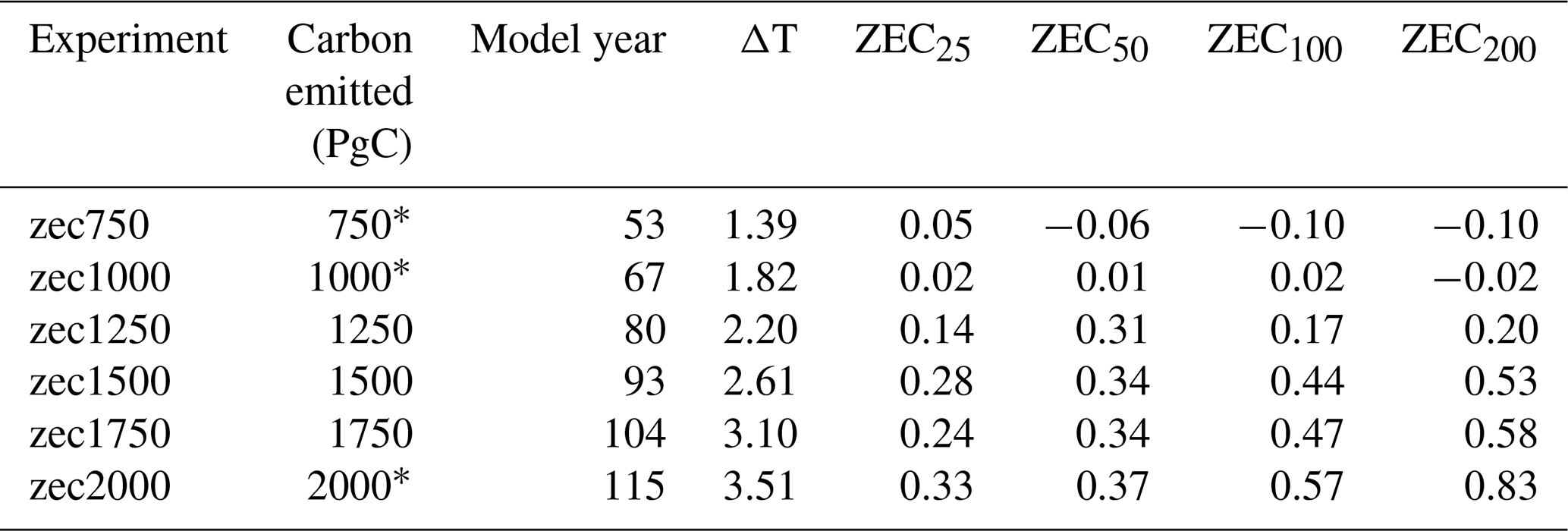
Throughout the paper, the names of ZECMIP and supplementary experiments include the amount of carbon emitted before branching, with text in lowercase (e.g. zec1000). Where particular ZEC results are shown, they are the difference between 20-year averages from the parent experiment centred on the branch point and the time from branching indicated by the subscripted value of the acronym (e.g. ZEC₅₀ will indicate the difference centred at 50 years), as defined in MacDougall et al. (2020).

In ZECMIP experiments, all atmospheric concentrations of non-CO₂ “greenhouse gases” and aerosols are held constant, and likewise the land use map is maintained with a preindustrial distribution. These idealised zero-emission experiments are different to plausible climate scenarios for the 21st century in which other gases and aerosols are also varying and influencing the climate, and, baring a global cataclysm, such an instantaneous transition to zero carbon emissions is perhaps unlikely. However, the results from ZECMIP experiments are expected to be the same as other plausible future climate stabilisation scenarios of corresponding branch point temperatures, such as those proposed by King et al. (2021). The usefulness of the ZECMIP-style experiments is their relatively straightforward configuration that can readily be adopted by any model with an active carbon cycle and even across different generations of CMIP.

3 Results and discussion

3.1 Global metrics

Figure 1 shows time series of several globally averaged climate metrics from 1pctCO2 and ZEC branches, along with the piControl. The time series of surface air temperatures from each ZEC branch are approximately linear (Fig. 1a). The overall rates of change are −0.035 °C per 100 years in zec750 and +0.315 °C per 100 years in zec2000, and the rates vary evenly across intermediate branches. As expected, atmospheric CO₂ concentrations drop in all ZEC branches but remain well above preindustrial values (Fig. 1b). Due to the slow response of the deep ocean and the persistent high atmospheric CO₂ values, ocean heat continues to increase in all ZEC branches (Fig. 1c). Most of the energy entering the climate system from the imbalance at the top of the atmosphere (TOA; Fig. 1d) is taken up by the ocean of each experiment. In the case of piControl, the non-zero TOA balance is consistent with the offset discussed in Ziehn et al. (2020); this offset was still present after a long spinup that stabilised the climate state, and the offset is not associated with any drift in the model. The responses of sea ice areas in the Arctic and Antarctic in the ZEC branches are distinct (Fig. 1e and f respectively). The Arctic sea ice area largely follows the changes in average global surface temperature (Fig. 1a). On the other hand, the Antarctic sea ice is largely unresponsive at the start of the 1pctCO2 and even the first 100 years of low ZEC branches. However, the longer integrations of the ZEC experiments presented here show reductions in Antarctic sea ice even in the zec750 branch, where after 200 years sea ice area is outside the range of variability from the piControl. The initial sea ice trajectory of zec2000 is close to that of 1pctCO2, indicating that the trajectory of the sea ice here at the zec2000 branch point is already “locked in” and independent of atmospheric forcing for several decades.

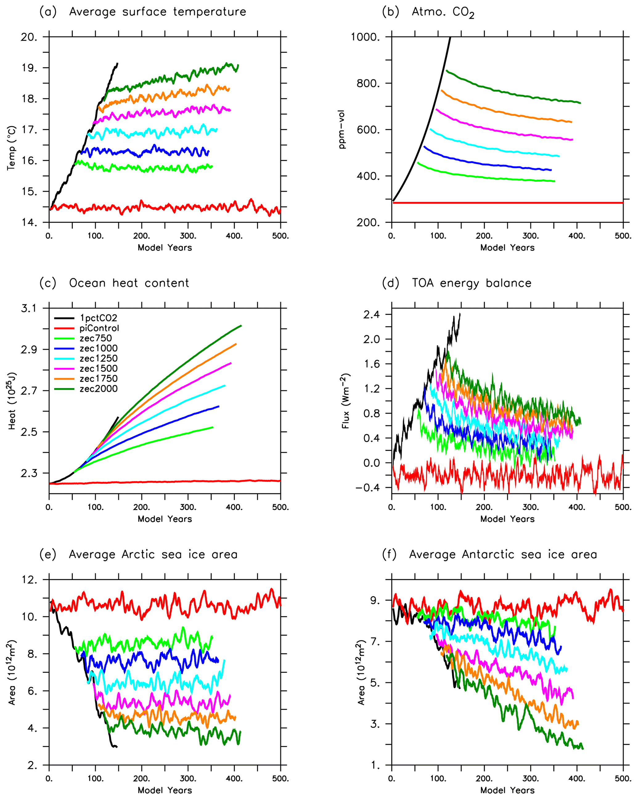
Figure 1 Global time series of (a) average near-surface temperature, (b) atmospheric CO₂, (c) ocean heat content, (d) top-of-atmosphere energy balance, and sea ice area of the (e) Arctic and (f) Antarctic from the 1pctCO2, ZEC branches and the piControl. Time series are smoothed with 5-year running averages.

3.2 Surface temperature changes

Figure 2 shows the evolution in zonally averaged near-surface temperatures in the 1pctCO2 and selected ZECMIP experiments. In 1pctCO2 there is a strong dominant warming in the Arctic responding to the increased climate forcing and global temperatures from higher atmospheric CO₂ (Fig. 2a). However, the Arctic and the Northern Hemisphere also cool as the atmospheric CO₂ decreases in low ZEC branches (Fig. 2b). The Arctic surface temperature changes appear to follow changes in the global temperature with local amplification from ice albedo feedback. In contrast, the Southern Ocean warms relatively slowly in 1pctCO2 and yet continues to warm in all ZEC branches, consistent with being the region with the greatest inertia in the climate system. For instance, while there is an overall global cooling in zec750, after 200 years from branching there is some warming in the same latitude band, 40–65° S, that stands out more clearly in zec1000 (Fig. 2b and c). At 65–70° S, the magnitude of warming in low ZEC branches is about the same as warming north of 60° S, whereas these poleward latitudes clearly dominate the warming in zec2000, corresponding to strong decreases in Antarctic sea ice and positive feedback on temperature, as seen in Fig. 1f. This slow response of the Southern Ocean has been identified in ocean observations and simulations of the current ocean state by Armour et al. (2016). Here we show the potential influence of this Southern Ocean response to the global climate in zero-emission scenarios.

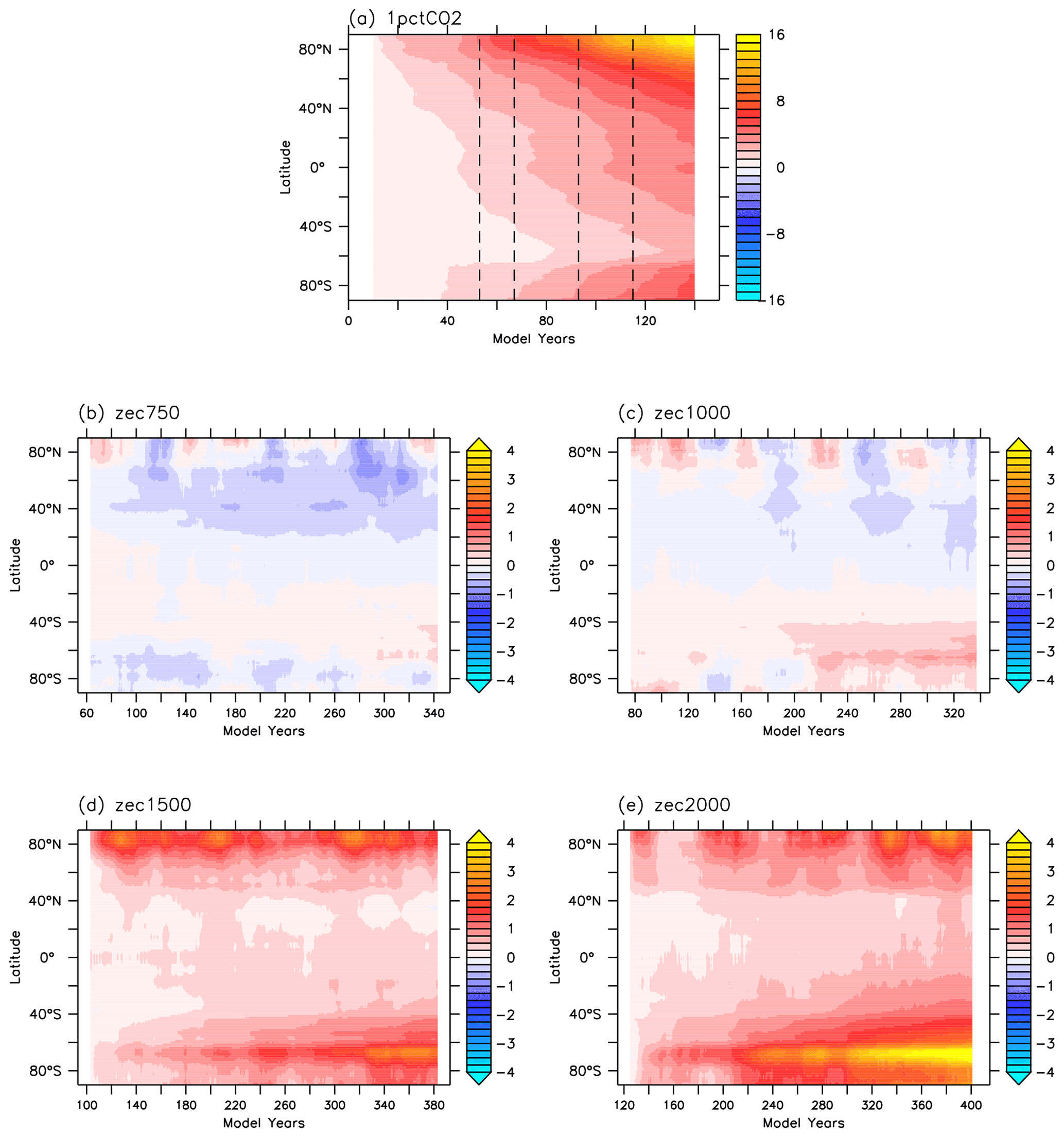
Figure 2 Changes in zonally averaged surface temperatures with time from 1pctCO2 and four of the ZEC branches investigated here. Differences from ZEC branches are with respect to the 20-year averages from 1pctCO2 centred on the branch point and smoothed with a 20-year filter. Dashed vertical lines in (a) indicate times that the ZEC scenarios show a branch from 1pctCO2.

Figure 3 shows the spatial distribution of the temperature changes in 1pctCO2 and ZEC branch experiments. In low ZEC branches (Fig. 3b and c) there is a broad Southern Ocean response that shows warming across the Atlantic and Indian sectors, extending north to ∼ 45° S, though not in the Pacific sector which is about neutral. High ZEC branches (Fig. 3d and e) show larger magnitudes of warming in the Southern Ocean that then drive global changes (note the expanding influences in the zonal time series; Fig. 2d and e). Warming is still evident across the broad regions of the Southern Ocean in high branches, but now the greatest temperature change is located in sea ice regions south of 60° S where changes now trigger positive ice feedbacks.

It is evident that neutral global responses of the lowest branches in Fig. 1 obscure significant regional changes. In particular, Figs. 2 and 3 demonstrate ongoing warming of the order of 1 °C after 300 years over the Southern Ocean that is largely compensated by cooling over large continental regions in low ZEC branches. In high ZEC branches, the change in temperature in these continental regions is small with respect to ocean and the Southern Ocean in particular. While there may still be some locations of cooling with decreasing atmospheric CO₂ in these high ZEC branches, the cooling is significantly less relative to the cooling in low branches. Also, cooling in these high branches is only found at locations within large continental areas. In contrast, Australia as a smaller continent tends to warm with the neighbouring oceans. Interestingly, one oceanic region shows less warming and even some cooling in zec1500 and zec2000 around the northern subtropical Pacific, which is relatively isolated to warming trends in the Arctic or Southern Ocean.

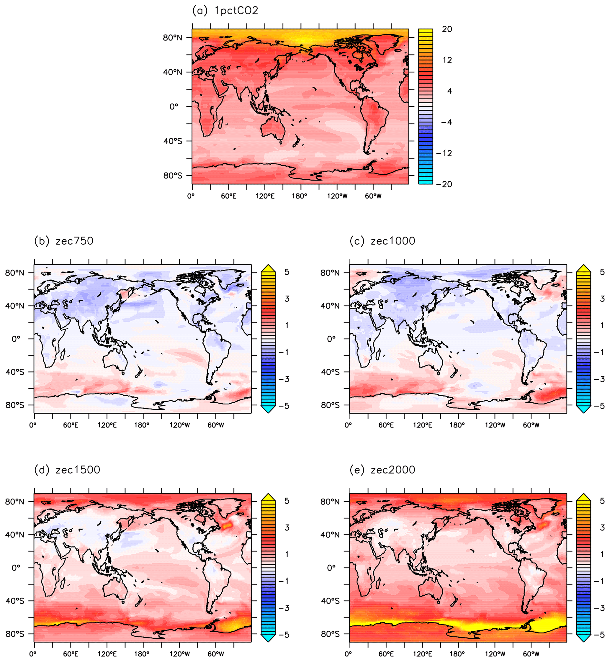
Figure 3 Change in surface temperatures. ZEC branch changes are averages of the last 20 years with respect to 1pctCO2 centred at the branch point (time difference, Δt=290 years), and 1pctCO2 changes are with respect to piControl (Δt=140 years).

Similar maps showing the change in surface temperatures over ZEC experiments from other ZECMIP models are presented by MacDougall et al. (2022). Maps of zec1000 50-year temperature change between the nine participating ESMs showed significant variability in the regional responses of ZEC simulations. Their Fig. 3 includes results from ACCESS-ESM1.5; however, unlike zec1000 in Fig. 3 here, there is no clear response from the Southern Ocean, whereas some other ZECMIP models indicate strong responses in the North Atlantic, probably associated with changes in the AMOC. As indicated in Fig. 2 here, the Southern Ocean response in zec1000 of ACCESS-ESM1.5 does not become apparent until about 200 years after branching and would not appear in the ZEC₅₀ results. Also, Gillett et al. (2011) explored zero-emission scenarios with the CanESM1 for centuries after branching from the year 2100 of the SRES A2 scenario (Meehl et al., 2007). While the global temperatures were about stable over these centuries, regional temperatures continued to evolve with as much as 3 °C of warming over the Southern Ocean, like those seen in high ZEC branches of ACCESS-ESM1.5 here. However, cooling over the Northern Hemisphere, particularly over high-latitude continental regions and the Barents Sea of the Arctic, balanced the southern warming in the global average of CanESM1.

ACCESS-ESM1.5, like many CMIP6 models, does not have an active ice sheet component, so these simulations will not include the effects of changes in meltwater from ice sheets. Purich and England (2023) show that the inclusion of meltwater around Antarctica in near-future scenarios has a relative cooling effect on surface temperatures across the Southern Ocean (or less warming) due to the reduction in the exchange of warmer, deep waters with the surface.

3.3 Subsurface changes

3.3.1 Overturning

Sections of global meridional overturning stream functions from different stages of 1pctCO2 are shown in Fig. 4. Overturning stream functions are shown with respect to both depth and density coordinates, and each indicates a decline in the strength of circulation of Antarctic Bottom Water. There is a greater influence on the deep bottom water circulation at 3000–4000 m in the second 50 years of 1pctCO2 than the first 50 (the change in Fig. 4c to e being greater than Fig. 4a to c). The density of the circulation close to the Antarctic coast, south of 60° S, decreases over the course of 1pctCO2 (Fig. 4b, d and f), breaking the coupling to the bottom circulation across the rest of the global ocean. In sections with both coordinates, the Deacon Cell in the Southern Ocean (55 to 40° S) is stronger and more extensive at the end of 1pctCO2.

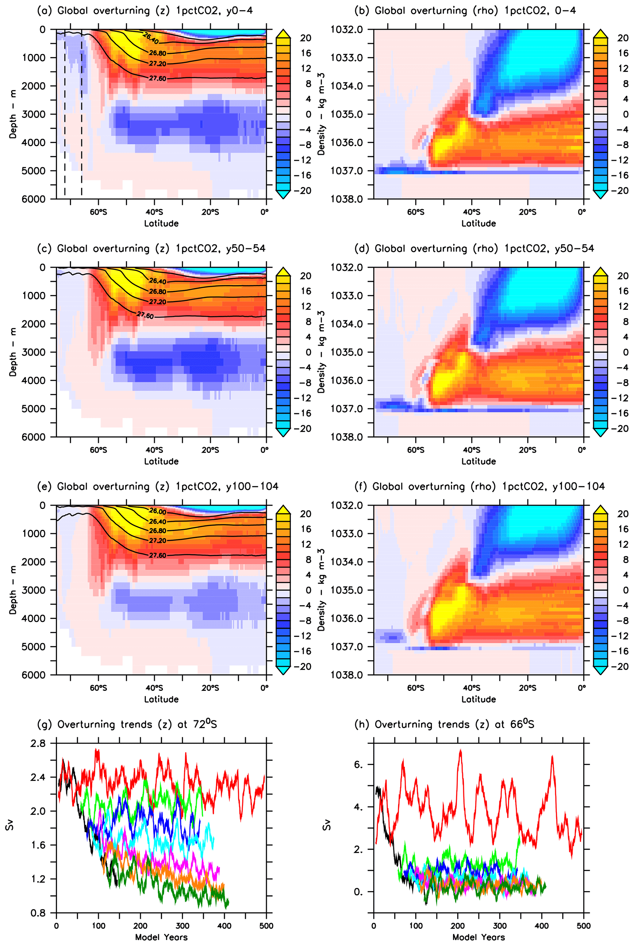
Figure 4 Global meridional overturning stream functions from 1pctCO2 calculated with respect to depth (left) and density (right, referenced to 2000 dbar, or a depth of ∼2000 m). The stream functions shown are 5-year averages: first 5 years of 1pctCO2 (top row), years 50–54 (second row) and years 100–104 (third row). The bottom row shows time series of overturning calculated with respect to depth at two positions near Antarctica (at 72 and 66° S, indicated by dashed lines in the top row) from 1pctCO2, piControl and ZEC branches smoothed with a 10-year filter (using the same colour scheme as Fig. 1).

The time series of the overturning shown in the bottom row of Fig. 4 are calculated as the magnitude of the minimum in the stream function in depth coordinates at two latitudes, 72 and 66° S. Variability is high in these overturning values, but with 10-year averaging persistent changes in all ZEC branches become evident, exceeding the significant decadal variability. Even low ZEC branches demonstrate that the small perturbations in average overturning relative to piControl do not recover in the 300-year integrations of the branches. Overturning time series in high ZEC branches at 72° S (Fig. 4g) continue to evolve after branching from 1pctCO2, indicating the slow response of deep overturning to changes in surface boundary conditions.

The circulation time series at 66° S appears to collapse as calculated in depth coordinates in Fig. 4h. Average overturning at this position in piControl is ∼ 4 Sv, albeit with significant decadal variability with a range that is also ∼ 4 Sv, and drops to ∼ 1 Sv in the low ZEC branches and even < 0.5 Sv in high branches, with no indication of any recovery in the 300-year integrations. However, overturning stream functions in density coordinates indicate circulation is ongoing at these latitudes. The timing of the branching of the lowest ZEC branches is about the time that the cell south of 60° S starts to shift to light densities, as seen in Fig. 4f.

Not having an active ice sheet component, ACCESS-ESM1.5 will not include the effects on circulation from changes in Antarctic meltwater. Li et al. (2023) and Purich and England (2023) show that the inclusion of Antarctic meltwater in near-future scenarios also acts to slow down overturning and the formation of Antarctic Bottom Water, indicating the meltwater impacts will enhance the changes in overturning and the ongoing changes in ocean tracers to what is presented here.

We focus here on the changes in the Southern Ocean. However, changes in the North Atlantic and AMOC have been identified as important features in other analyses of ZEC scenario experiments. MacDougall et al. (2022) assessed regional responses in zec1000 from ZECMIP models. One of the significant features at 50 years (ZEC₅₀) was in the North Atlantic, which was cooler in some of the models assessed. ACCESS-ESM1.5 was included in this assessment, and the Southern Ocean presented here was not prominent. The zec1000 experiment is a relatively low branch of the ZEC scenarios presented here, and 50 years is shorter than the timescale that the Southern Ocean response here becomes apparent.

Schwinger et al. (2022) also assessed the impact of AMOC changes, testing various ZEC scenarios with the NorESM2 (Seland et al., 2020) and assessing the response of multiple high-emission ZEC branches like done here with ACCESS-ESM1.5 and also overshoot scenarios where negative emissions are used to reduce the CO₂ and climate forcing. Schwinger et al. (2022) found significant AMOC responses: temperatures cooled as AMOC weakened and temperatures warmed as AMOC recovered and strengthened. Interestingly, the NorESM2 was included in the multi-model analysis in MacDougall et al. (2022), but the NorESM2 response was not so significant there, possibly because the response in Schwinger et al. (2022) is on centennial timescales and did not show a strong ZEC₅₀ response in zec1000.

3.3.2 Tracer distributions

The changes in the circulation and surface forcing from the increased climate forcing of 1pctCO2 initiate long-term changes in the distribution of subsurface ocean properties that continue even once the climate forcing decreases and stabilises in the ZECMIP experiments. Figures 5, 6 and 7 show changes in zonally averaged sections of temperature, salinity and oxygen in the 1pctCO2, zec750 and zec2000, as well as time series of tracers at selected positions from 1pctCO2, piControl and all ZEC branches. Figure 8 demonstrates the changes in the ocean depth of heat uptake in the different ZEC branches.

The time series (panels j, k and l of Figs. 5, 6 and 7) demonstrate that even small changes in circulation and surface forcing of low ZEC branches are sufficient to drive ongoing subsurface changes in heat, salt and oxygen, even if these changes are not expressed at the surface. There is a monotonic increase in the rate of change in the subsurface warming with ZEC branches, and the fastest warming is in the highest ZEC branches at all positions shown in Fig. 5. Similar responses are seen in oxygen time series (Fig. 7), where high branches generate greater decreases in oxygen. with exceptions that are discussed further below. For the time series of each tracer at 20° S (panel l of each figure), while there are consistent signals across the experiments presented, the magnitudes of low-frequency variability are similar to these signals, and a larger 30-year filter is applied to reduce this variability.

Changes in the temperature sections of 1pctCO2 (Fig. 5d and g) are predominately near the surface north of 40° S, with deeper warming near Antarctica down to 2000 m and in the Southern Ocean at 45–50° S down to 1000 m related to a poleward shift in water masses. In contrast, temperature changes in ZEC branches are predominantly at depth, ∼ 500–1500 m north of 60° S and deeper to the south, with less change at the surface.

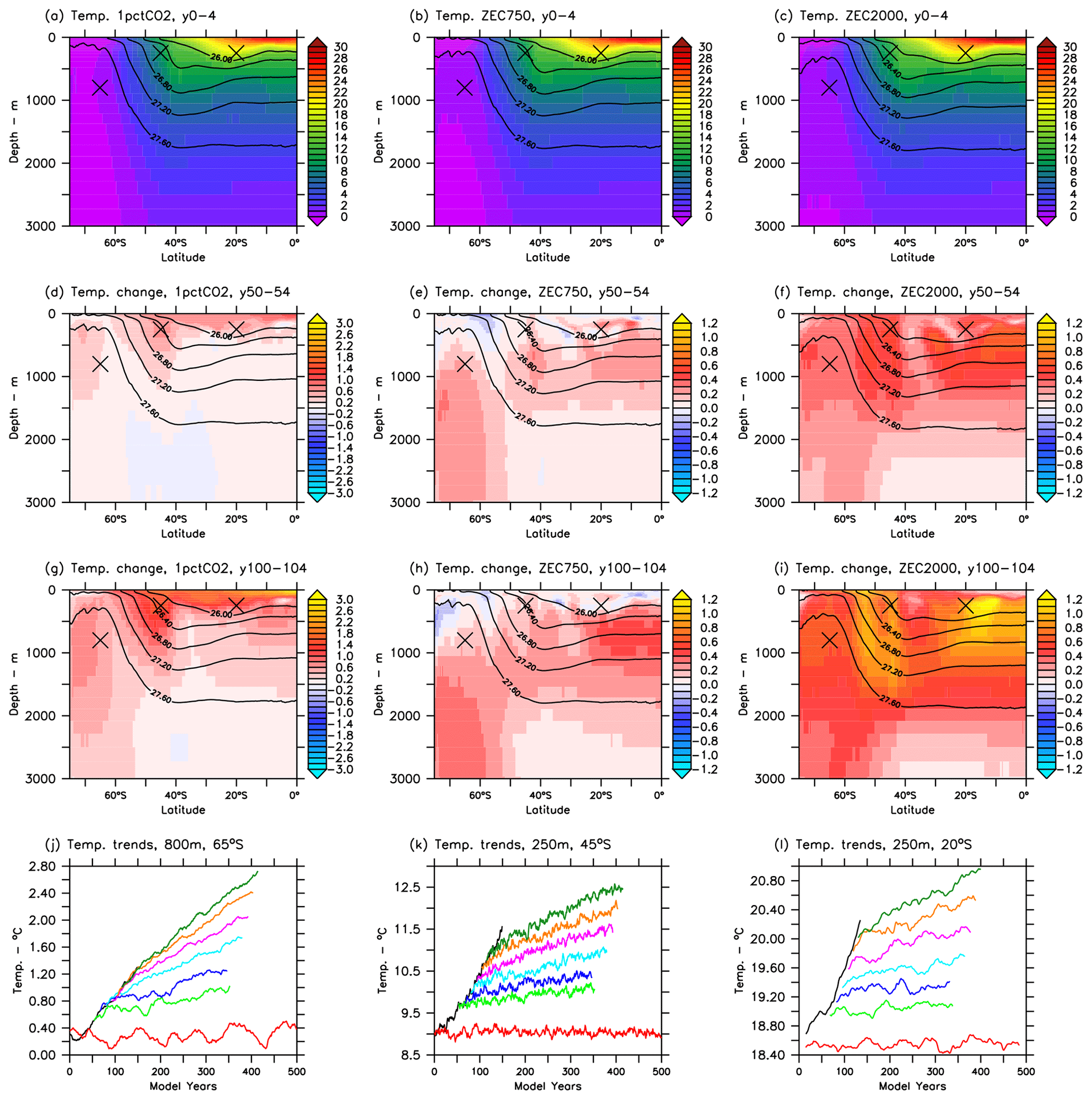
Figure 5 Changes and time series in average zonal sections of temperature. The top row shows zonally averaged sections for the first 5 years from 1pctCO2 (left) and ZECMIP branches after emitting 750 PgC (middle) and 2000 PgC (right). The second and third rows show changes in zonally averaged sections from the same experiments after 50 and 100 years respectively. Contours indicate zonally averaged potential densities. The bottom row shows time series of subsurface temperatures in the Southern Ocean (at 65, 45 and 20° S, at positions indicated) from 1pctCO2, piControl and ZEC branches (same colour scheme as Fig. 1). Time series at 65 and 45° S are filtered by 1 year, and series at 20° S are filtered by 30 years.

The uptake of heat in 1pctCO2 and selected ZEC branches is shown in Fig. 8 as changes in the globally averaged temperature with depth and time within each experiment. Consistent with the ocean heat content in Fig. 1c, temperature increases are much larger in high ZEC branches; also, the distribution of temperature increase is shallower in high branches. At the end of the 300 years with zero emissions, the peak temperature increase in zec2000 is at ∼ 800 m, whereas in zec750 it is at ∼ 1200 m. While temperature still increases below ∼ 200 m in zec750, there is some cooling in the upper 100 m in response to the decreasing atmospheric CO₂ and reduced climate forcing. In contrast, in zec2000, the highest temperature increase is closer to the surface and has a greater influence on the upper ocean and surface.

Figure 6 shows changes in zonal averages of salinity from 1pctCO2 and selected ZEC branches. The changes in zonal salinity in 1pctCO2 vary spatially and are distinct from temperature changes, with freshening in the upper ocean near Antarctica and increasing salinity below 800 m. In zec750, the main change in the salinity section is a freshening between 40 and 60° S in the upper 1000 m. In zec2000 the ongoing salinity changes are more uniform, with a general freshening of the upper ocean above a band of increasing salinity below 500 m near Antarctica and extending north of 50° S at depths between 1000 and 2000 m.

Changes in the distribution of salinity are somewhat slower to become evident in 1pctCO2. For instance, in the time series for the positions shown in panels j, k and l of Fig. 6, the salinity differences between zec750 and the control are minor even after 300 years. Trends in temperature at the same positions were more distinct from the control and showed growing differences after 300 years. The transient response of salinity at 25° S and 250 m in 1pctCO2 is an increase in salinity. However, in all ZEC branches salinity decreases, albeit with significant interannual variability, indicating a recovery in the atmospheric circulation and precipitation under zero-emission climates with decreasing atmospheric CO₂.

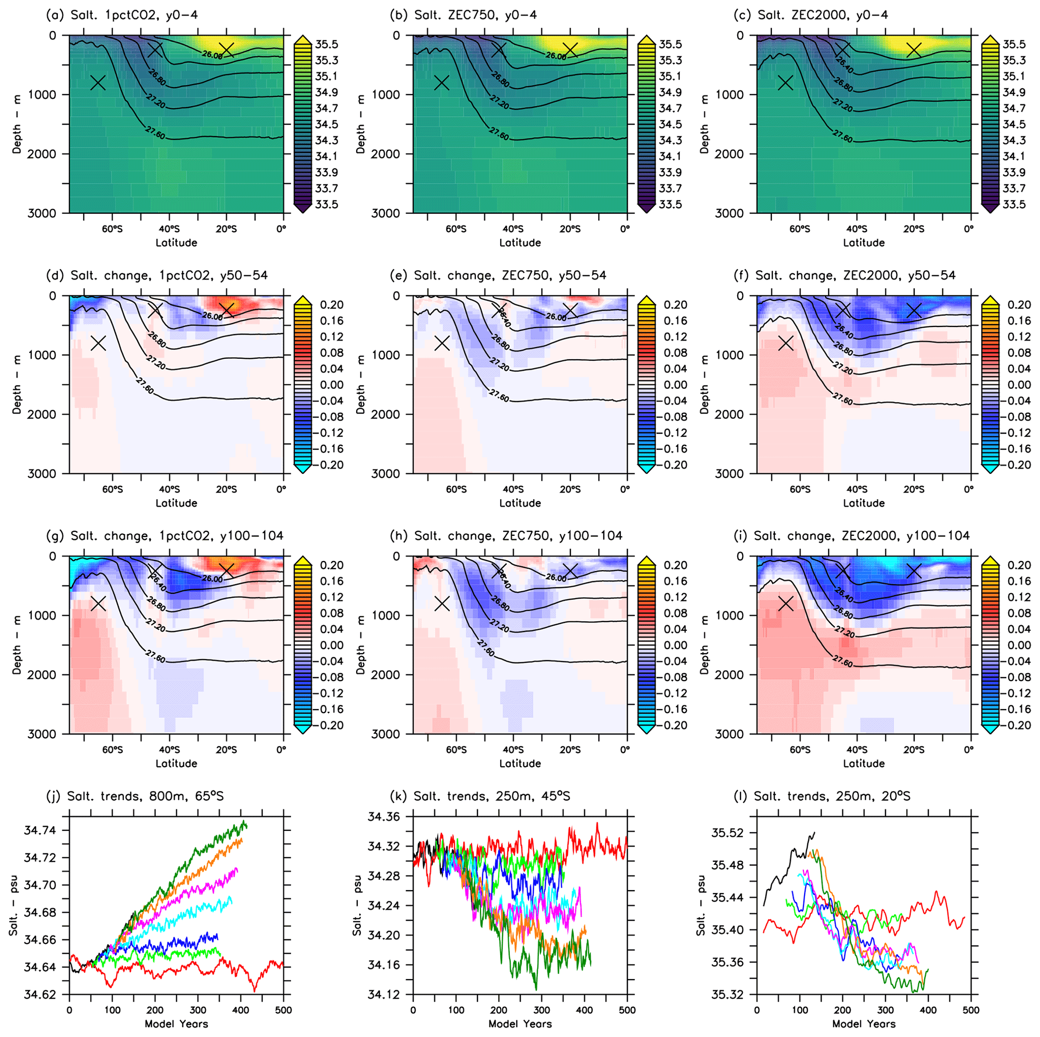
Figure 6 Changes and time series in average zonal sections of salinity, with the same layout as Fig. 5.

The distribution and responses of ocean biogeochemical tracers (for example oxygen; Fig. 7) are distinct from both heat and salinity due to the different distributions of tracer sources and sinks, both at the ocean surface and in the interior. Hence, the mean fields of biogeochemical tracers are distinct from physical tracers and are impacted in different ways by the changes in ocean state and circulation. As the strength of deep Antarctic overturning weakens, there is a decrease in the supply of oxygen from surface waters into all depths of the interior of the Southern Ocean. Local exceptions to the general decline in oxygen include water between 0 and 1000 m at 50–60° S in low ZEC branches where oxygen likely increases due to the greater influence from southern oxygen-rich surface water and less from oxygen-poor waters because of changes in circulation and global stratification (panels e and h of Fig. 7). There is also an increase in subsurface oxygen below equatorial regions, north of 10° and below 500 m, where productivity declines in warmer climates of both zec750 and zec2000. Reduced productivity and export of organic material reduce the consumption of subsurface oxygen in these regions, driving this oxygen increase.

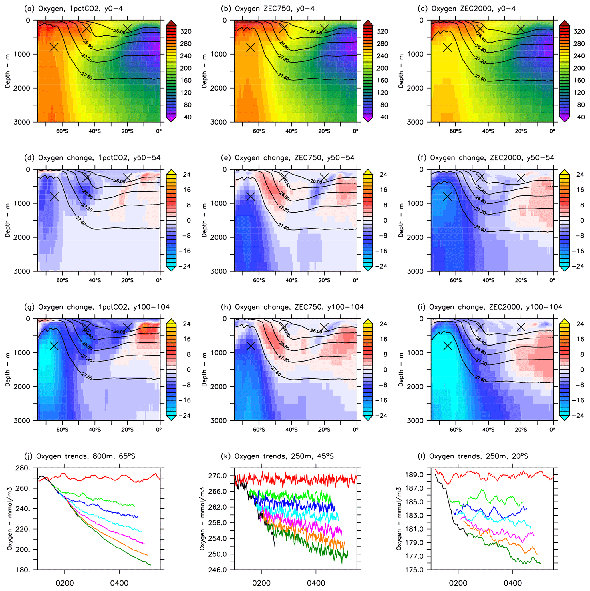
Figure 7 Changes and time series in average zonal sections of oxygen, with the same layout as Fig. 5.

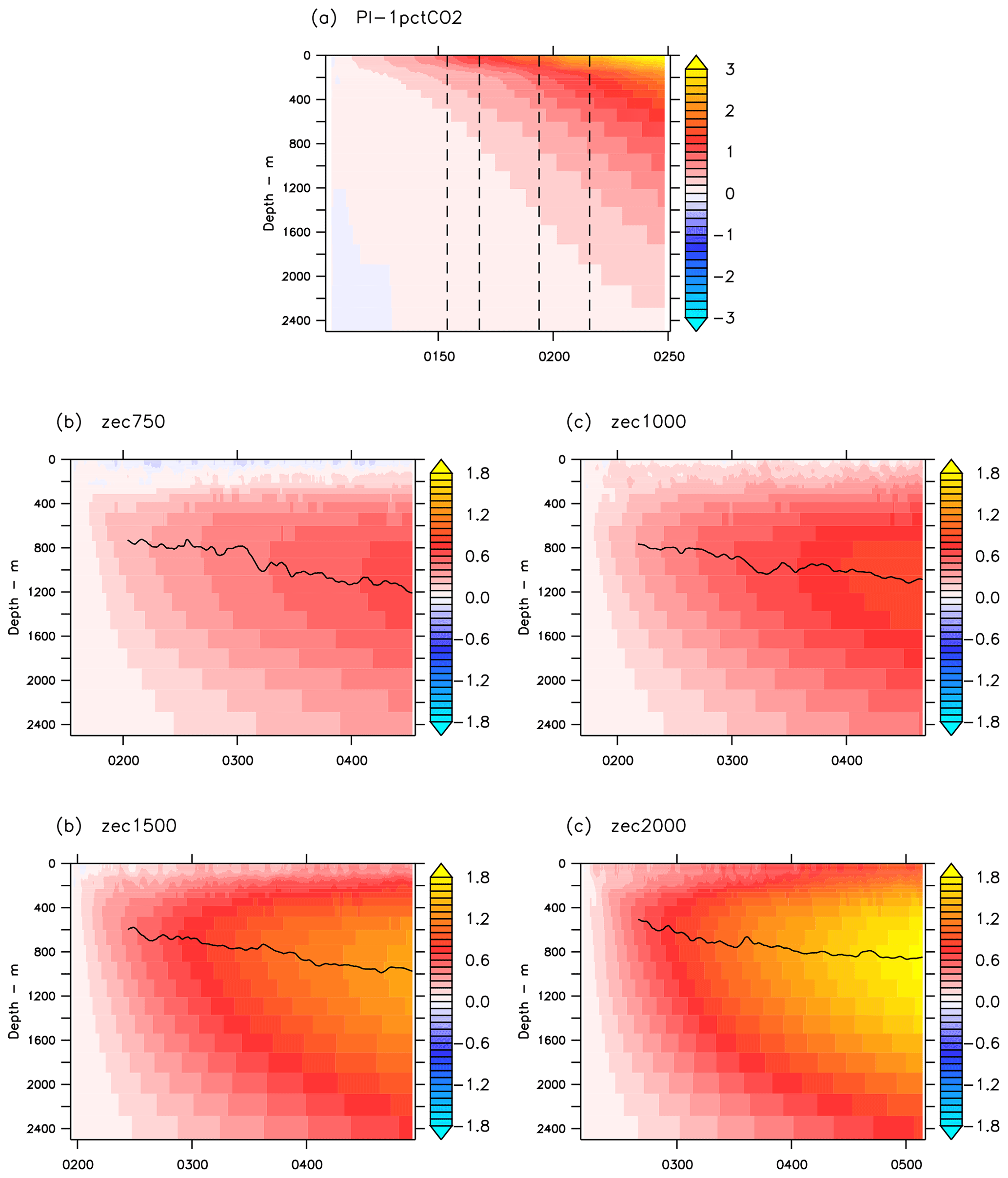
Figure 8 Heat uptake of the whole ocean as a function of depth and time, shown as changes in global averages of temperature within each experiment. Dashed vertical lines in panel (a) indicate the times that the ZEC experiments in (b)–(e) branch from the 1pctCO2. Solid lines overlain indicate the depth of maximum change in temperature in ZEC branches.

3.4 CO₂–temperature trajectories

Figure 9 shows the trajectories of 1pctCO2 and ZEC branches with respect to CO₂ and global average near-surface temperatures. The trajectories of these branches are consistent with climates approaching their equilibrium states after initial perturbations and warming in the 1pctCO2 experiment before branching. Overlying these experiments are temperatures corresponding to the transient climate response (TCR) and equilibrium climate sensitivity (ECS) of ACCESS-ESM1.5, calculated with the logarithmic relationship of CO₂ and radiative or “climate forcing” (Myhre et al., 1998) and assuming a constant climate feedback parameter (λ, Wm⁻² °C⁻¹). Both TCR and ECS are expressed as the global warming associated with a doubling of atmospheric CO₂, and TCR is typically substantially less than a model's ECS. The TCR and ECS for ACCESS-ESM1.5 are 1.95 and 3.87 °C respectively (Ziehn et al., 2020). The trajectory of 1pctCO2 in Fig. 9 starts from the lower left (285 ppm, 14.3 °C) and moves to the right, generally following the TCR (the TCR is defined by the response of 1pctCO2 at 70 years). As ZEC experiments branch their CO₂–temperature trajectories turn left with decreasing CO₂ and move towards the ECS over the 300 years of integration. Consistent with the time series of the surface temperatures in Fig. 1, the trajectories of the lowest ZEC branches have stabilised near their equilibrium climates by the end of the 300-year integration and are close to ECS values. Climate states of higher ZEC branches are still evolving and with further model integration are expected to also stabilise at an equilibrium climate temperature, though this may take several centuries or longer for the highest branches.

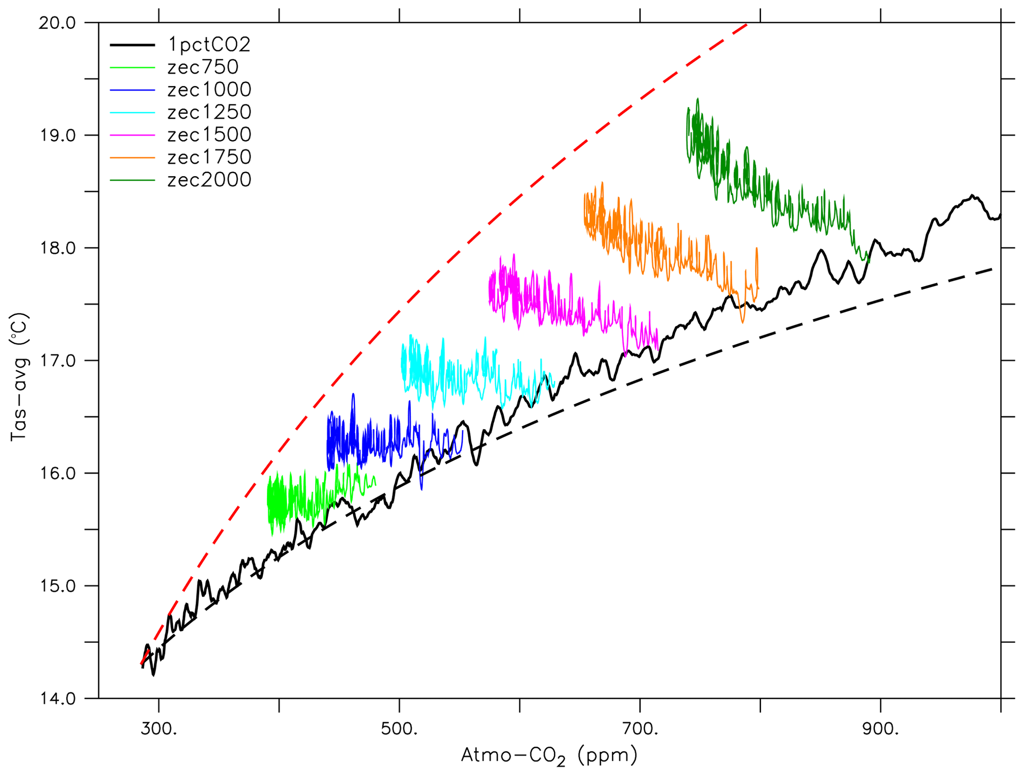
Figure 9 Time series of globally averaged surface temperatures with respect to atmospheric CO₂ for the 1pctCO2 and ZEC branches. Dashed lines indicate temperatures corresponding to the TCR (black) and ECS (red).

3.5 Slab model

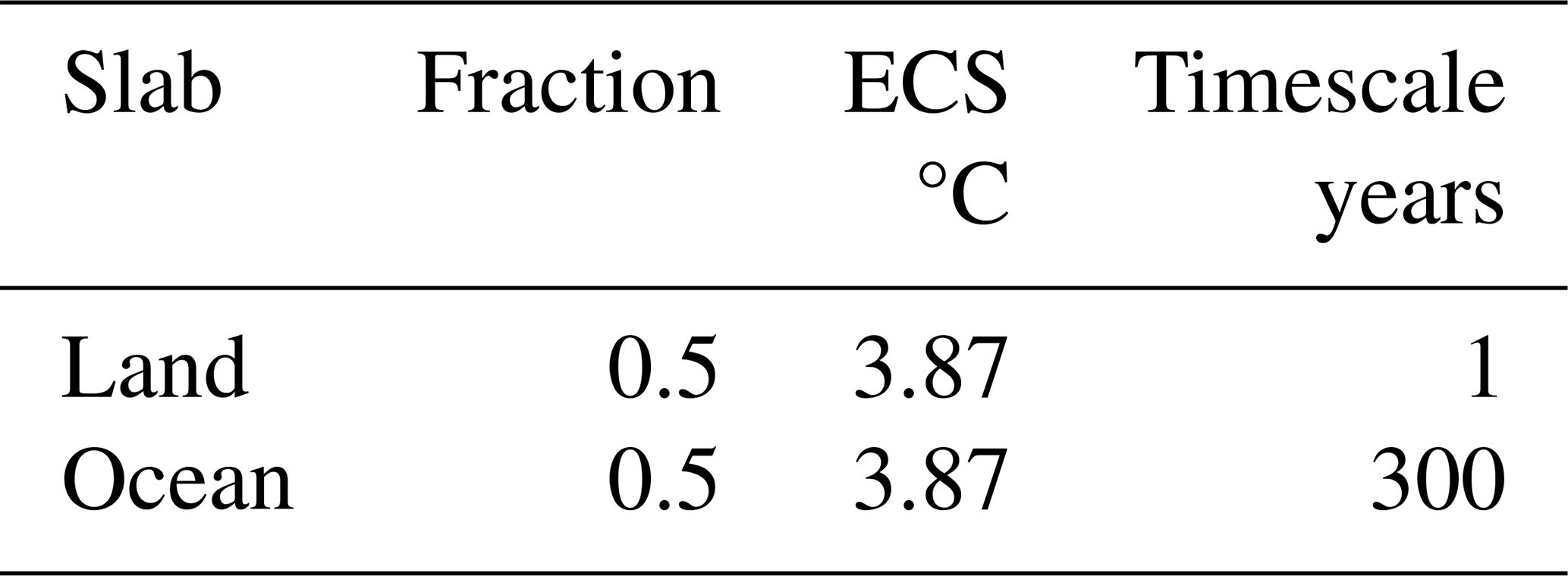
As a way to explain and understand the global temperature trajectories in 1pctCO2 and ZEC branches, a simple model of independent slabs with different inertias, conceptually representing responses from the land and ocean, is used to replicate these trajectories. There are other simplified models that have been constructed to emulate full ESMs, such as “energy balance models” (e.g. Geoffroy et al., 2013), though the slab model based on temporal responses is quite adequate to reproduce the average temperatures from ACCESS-ESM1.5 here. Global temperature is an average of just two slabs that both approach the same equilibrium temperature anomaly determined by time-evolving atmospheric CO₂, as diagnosed from ACCESS-ESM1.5 simulations. Various processes related to the heat uptake and response of surface temperature for both the land and the ocean are parameterised in the timescales and inertias assumed. These global temperature trajectories are shown in Fig. 10, where the timescale of the land slab is 1 year and effectively follows the equilibrium temperature, while the ocean timescale is 300 years. See Appendix A for more details and discussion on the model setup. These timescales for land and ocean were determined by fitting to global temperatures of 1pctCO2. Temperatures of slab models with ocean timescales of 100 and 500 years are also shown which over- and underestimate the 1pctCO2 temperature time series. The slab model captures both the 1pctCO2 and the key trends of the ZECMIP trajectories shown, namely the slight decrease in zec750, neutral zec1000 and increases in higher ZEC branches.

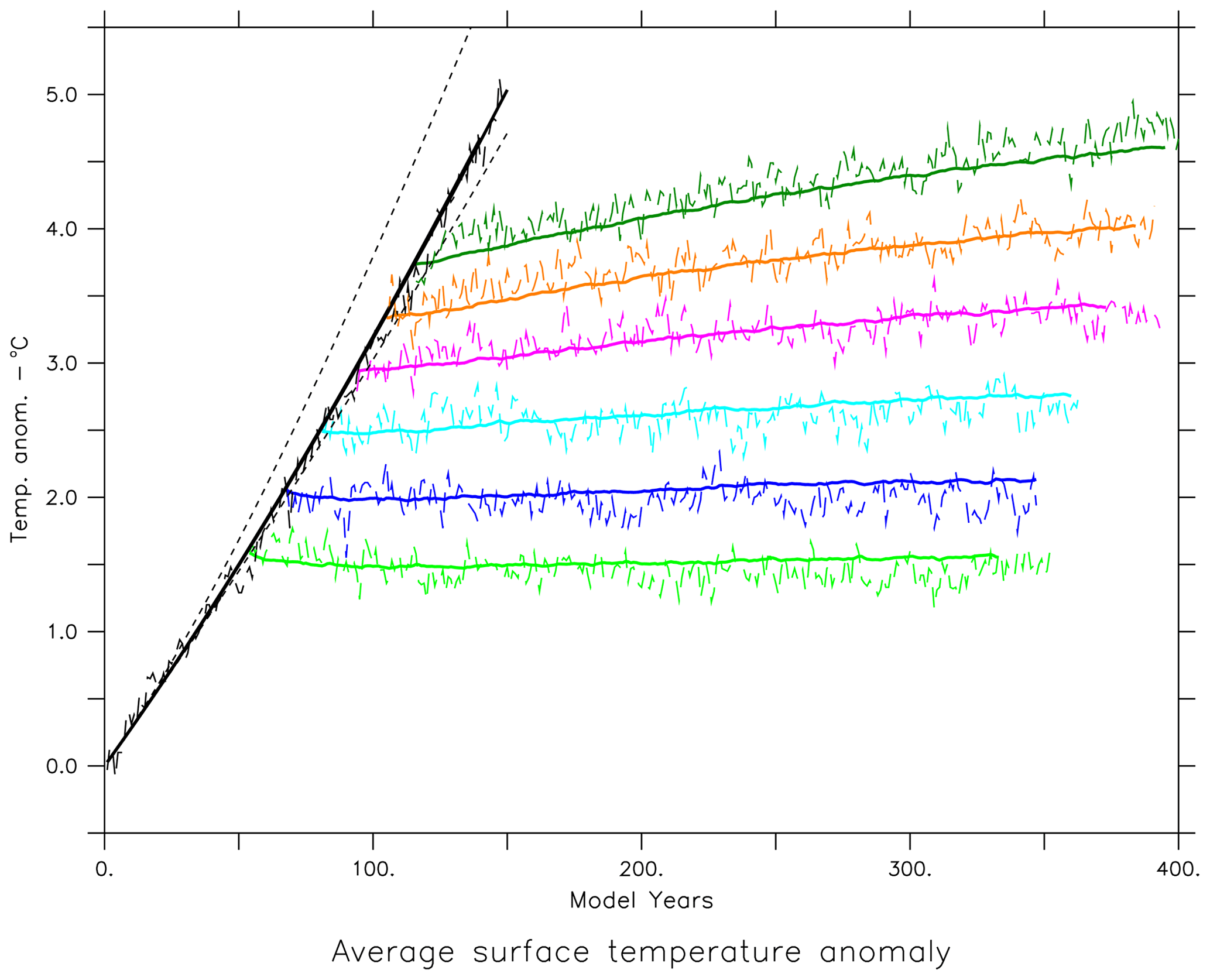
Figure 10 Global time series of average surface temperature for the 1pctCO2 and ZEC branches from ACCESS-ESM1.5 (dashed lines) and slab model (solid lines, same colour scheme as Fig. 9). Dotted black lines show slab-model temperatures for 1pctCO2 with ocean timescales of 100 and 500 years.

Being able to replicate the global temperatures with this slab model demonstrates that the ZEC trends found with ACCESS-ESM1.5 are due to the inertial response of the ocean within the climate system, which (from the zonal temperatures of Fig. 2) can be attributed to the Southern Ocean. In this way the Southern Ocean is like the “freight train” of the climate system; once the Southern Ocean has started warming noticeably in transient scenarios it will continue warming and even affect the global climate after switching to zero emissions (as shown in Fig. 2). At this point, the long-term global temperature trajectory will not be reversed by zero-emission scenarios but rather require ongoing negative emissions and extraction of CO₂ from the climate system.

Climate “tipping points” can be considered thresholds at which the climate changes to a new state and potentially continues to evolve without applying further increases in climate forcing; for example the loss of ice sheets or permafrost, forest dieback, or shutdown of overturning circulations. Some of this tipping point behaviour is present in results presented here, though there are no new processes and the fanning out of global temperature trends in Fig. 1 indicates this does not occur at a single point as such, but rather it is a transition, where the later the branching off from the 1pctCO2 experiment or more CO₂ emitted before switching to zero emissions, the stronger the ongoing warming. This general result does not preclude other local tipping points to be crossed in the process, notably changes to circulation and structure of the Southern Ocean during the warm epoch, for example, the point at which the average Antarctic sea ice area starts to decrease in Fig. 1f or changes in overturning stream function in Fig. 4h. While the Southern Ocean and its climate response may not fit an example of a tipping point, its potential to drive ongoing warming with global impacts, supported by results of the slab model and without additional climate forcing, suggests it should be considered in discussions of regions and processes of particular interest for climate change.

3.6 Multi-model comparison

3.6.1 Global surface temperatures

A curious observation from ZECMIP was the range of responses from the different models, such as in Fig. 6 of MacDougall et al. (2020). In particular, how some models (ACCESS-ESM1.5 and UKESM1-0-LL) showed positive ZEC values in zec2000, while other models (GFDL-ESM2M, MIROC-ES2L and CanESM5) were negative.

The slab model that is primarily tuned to ACCESS-ESM1.5 is now driven with CO₂ diagnosed from other ZECMIP ESMs that simulated all three ZECMIP type-A experiments to assess how the physical component of ACCESS-ESM1.5 would respond if it were coupled with different biogeochemistry and how much of the ZEC response is dependent on the physical versus the biogeochemical components. Atmospheric CO₂ data from each ZECMIP model, which are available at http://terra.seos.uvic.ca/ZEC, last access: 2 July 2023 (Eby, 2023), are used to force the slab model, and slab-model temperatures are compared to the temperatures from the original ZECMIP models. Figure 11 shows results of these comparisons for the three ESMs that submitted output for all three ZECMIP branches. The ECS of the slab model for these comparisons is made to match the ECS of each model as reported in MacDougall et al. (2020), with the one exception for the GFDL-ESM2M where a higher value of 2.9 °C is used to approximately match the original zec2000 temperatures instead of the reported 2.4 °C. This is consistent with Paynter et al. (2018), who found the GFDL-ESM2M had a higher ECS in multi-millennial simulations due to changes in the climate feedback parameter associated with ongoing evolution in sea surface temperature and atmospheric state. The slab ECS is adjusted primarily so results are on the same scale as the other models. Otherwise, the slab is tuned to the physical response of ACCESS-ESM1.5.

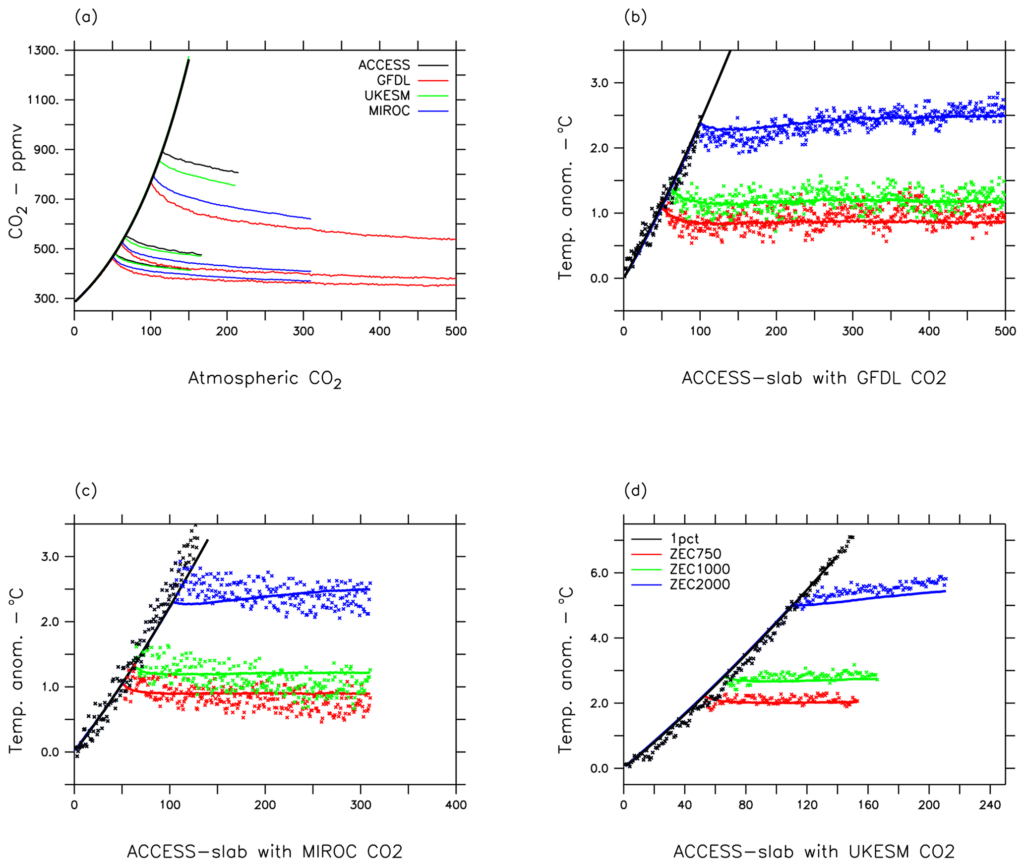
Figure 11 Global time series of (a) atmospheric CO₂ and average surface temperatures for the 1pctCO2 and ZEC branches from ESM models submitted to the ZECMIP: (b) GFDL-ESM2M, (c) MIROC-ES2L and (d) UKESM1-0-LL. Annual averages of original model temperatures are shown as individual points; slab-model temperatures are solid lines.

The first observation from Fig. 11 is the overall similarity of the response of the slab model with the temperatures found to original GFDL-ESM2M and UKESM1-0-LL results. In both of these models, the global temperatures in zec2000 continue to rise on a centennial timescale, like ACCESS-ESM1.5, despite the lower CO₂ values (Fig. 11a). While the centennial responses of the ZECMIP models are similar, their ZEC₅₀ values are quite different and even of opposite sign, as shown in Fig. 6 of the ZECMIP paper (MacDougall et al., 2020) and calculated again here (Table 2) and discussed below. These disparate results can be associated with the models having different responses at shorter, annual to decadal timescales.

The GFDL-ESM2M has the largest drawdown of CO₂ of the models shown (Fig. 11a), and there is cooling in both the original GFDL-ESM2M and slab models in the first decades of all ZEC branches (Fig. 11b). However, beyond 100 years, the centennial responses of the models dominate and temperatures rise in original GFDL-ESM2M results and the slab for zec2000. There is a similarity in the physical response of these two models in that there are similar relative trends in ZEC values for all branches in Table 2. The long-term ZEC of the GFDL-ESM2M is positive and increases like the original ACCESS-ESM1.5, despite different CO₂ responses. Note that both GFDL-ESM2M and ACCESS-ESM1.5 have MOM5 as their ocean component, albeit with different grids and parameterisations.

The UKESM1-0-LL has a relatively slow temperature response to the changing CO₂ even in the course of 1pctCO2 where the original UKESM1-0-LL temperature increases are apparently delayed with respect to the slab (Fig. 11d). This lagged response is also seen at the start of each ZEC branch, where temperatures continue increasing for the first decade, associated with the previous increasing CO₂ from before the branch points. Consequently, ZEC₅₀ calculated with UKESM1-0-LL is significantly positive, even for the lowest zec750 branch which otherwise shows a relatively neutral response on the centennial timescales in both the original UKESM1-0-LL and slab results. Slab ZEC temperatures with the UKESM1-0-LL CO₂ that do not have this lagged response are negative for zec750 and zec1000 and positive to zec2000, whereas UKESM1-0-LL ZEC values are all positive (Table 2).

The MIROC-ES2L results are distinct relative to the other models here. The global temperatures in original MIROC-ES2L results are decreasing on centennial timescales for all ZEC branches. The MIROC-ES2L temperature response closely follows changes in CO₂ and climate forcing. In contrast, the slab tuned to ACCESS-ESM1.5 has a slower response and shows rising temperatures in zec2000 with the same MIROC-ES2L CO₂. In Table 2, the ZEC₅₀ values of the ACCESS slab are similar to the original MIROC-ES2L values, within ∼ 0.1 °C, whereas MIROC-ES2L ZEC₂₀₀ values are 0.2 to 0.3 °C lower than the ACCESS slab values.

Table 2 ZEC values from ZECMIP model temperatures submitted to MacDougall et al. (2020), as well as ZEC values from the ACCESS-ESM1.5 slab with CO₂ diagnosed from ZECMIP models. Values are the differences between 20-year averages centred at the year of the ZEC branch (or 10-year average in the case of UKESM1-0-LL ZEC₁₀₀ values), relative to the 20-year average from the respective 1pctCO2 centred at the branch point. n/a: note that UKESM1-0-LL ZEC branches were only integrated for 100 years, so ZEC₂₀₀ values were not available.

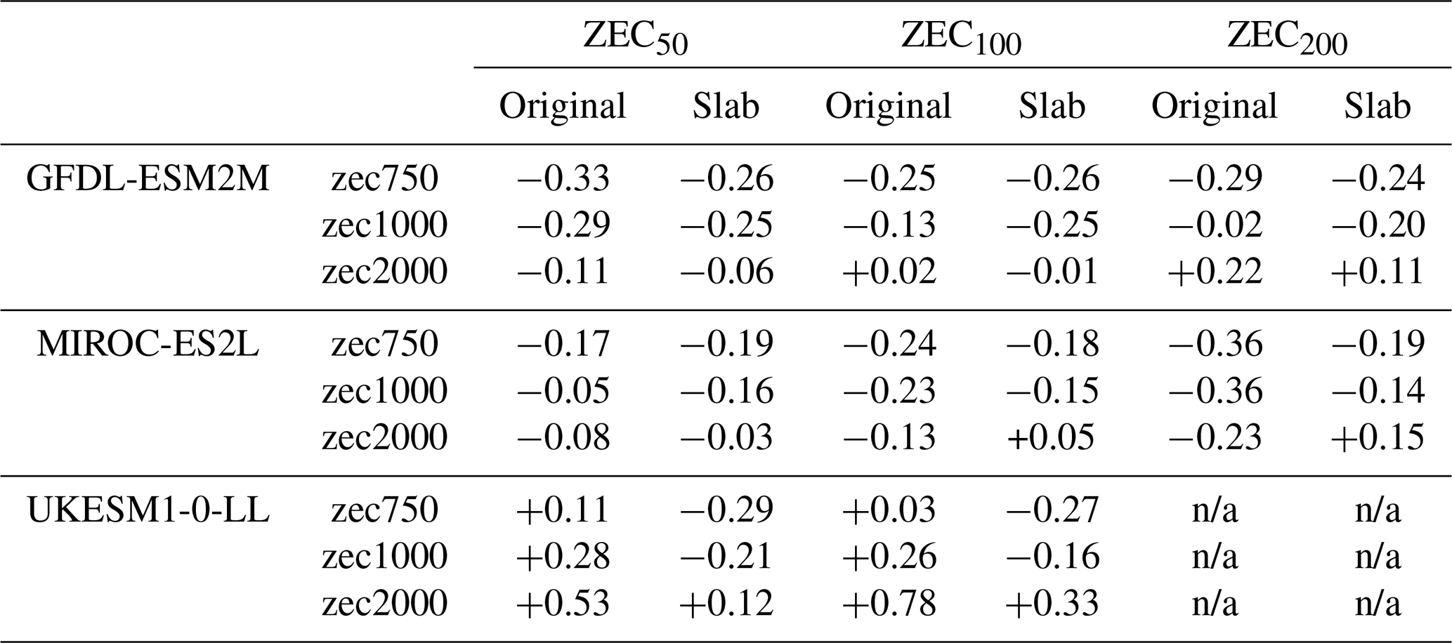
From these comparisons, the different long-term responses shown in ZECMIP models largely depend of properties of the physical climate models with some influence of the carbon cycle on the decadal responses and low ZEC branches, noting that while ZEC values from zec1000 with ACCESS-ESM1.5 are zero (within uncertainty; Table 1), values from the slab tuned to ACCESS-ESM1.5 but with CO₂ diagnosed from zec1000 experiments with other ZECMIP models are all negative (Table 2). Overall, ACCESS-ESM1.5, GFDL-ESM2M and UKESM1-0-LL are similar, showing significant responses at centennial timescales, in contrast to MIROC-ES2L where temperatures cool as atmospheric CO₂ decreases. Details in the physical response, such as the relative contributions at annual to decadal timescales, affect the values calculated for ZEC₅₀. The rapid CO₂ uptake of the GFDL-ESM2M leads to negative ZEC₅₀ values in each branch in both the original model and the slab, whereas the lagged, decadal response in the UKESM1-0-LL produced positive ZEC₅₀ values in the original model but not the ACCESS slab.

These observations indicate that while ZEC₅₀ values are relevant on policy timescales, where modifications to current rates of CO₂ emissions may modify the expected ZEC₅₀, this metric can be a poor representation of the complete response of ESMs, and later ZEC values are useful to consider for long-term implications for the climate state. Frölicher et al. (2014) also found variable responses over long integrations of ESMs under zero-emission scenarios, finding changes in the influence of the ocean on the global climate and even varying ECS values on multi-century timescales.

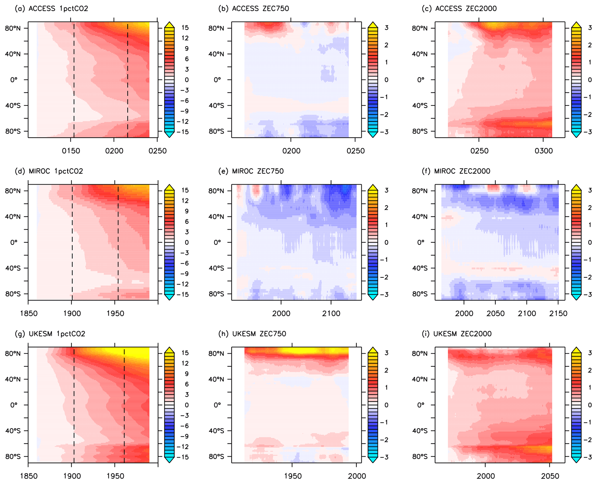
Figure 12 Changes in zonal average temperatures in 1pctCO2 (left), zec750 (middle) and zec2000 (right) from ZECMIP ESM models: ACCESS-ESM1.5 (top), MIROC-ES2L (centre) and UKESM1-0-LL (bottom). Temperatures are smoothed by averaging over 20 years and are differenced with respect to 20 years of 1pctCO2 centred at the branch point of each experiment, indicated by dashed lines of the 1pctCO2 panel for each model.

3.6.2 Zonal surface temperatures

In the case of ACCESS-ESM1.5, the temporal evolution of zonal average temperatures, as shown in Fig. 2, clearly indicates the latitudes of the Southern Ocean to be regions with a slow response in 1pctCO2 and also ongoing warming in all ZEC branches tested. Figure 12 is an equivalent plot of zonal average temperatures with available ZECMIP ESMs, namely MIROC-ES2L, the UKESM1-0-LL and ACCESS-ESM1.5. Note that these results are based on the experiments originally submitted to ZECMIP and available on the ESGF (World Climate Research Program, 2023). In the transient 1pctCO2 phase (left column), the broad patterns in the temperature changes are similar, each model shows the greatest warming in the Arctic and slowest warming around the Southern Ocean, though Arctic warming is greater in the UKESM1-0-LL by several degrees. There is an overall global neutral response in the 100 years of zec750 for ACCESS-ESM1.5 and UKESM1-0-LL and cooling in MIROC-ES2L (middle column), and temperature changes related to slow modes of climate variability are evident. ACCESS-ESM1.5 showed warming at Southern Ocean latitudes in zec750 before in Fig. 2, but this manifests on timescales longer than the 100 years shown here. In zec750, the Arctic region cools in MIROC-ES2L but continues to warm in UKESM1-0-LL. In zec2000 (right column), consistent with Fig. 11, there is broad warming in ACCESS-ESM1.5 and UKESM1-0-LL but cooling in MIROC-ES2L. The Southern Ocean features prominently as a region of ongoing warming in both ACCESS-ESM1.5 and UKESM1-0-LL, particularly at latitudes under the influence of sea ice south of 60° S. The Arctic in the UKESM1-0-LL shows less warming than ACCESS-ESM1.5 in zec2000, though the UKESM1-0-LL has warmed more here in the transient experiment before branching. Even in MIROC-ES2L, which shows overall cooling in zec2000, the Southern Ocean is a site of local warming, in this case at latitudes predominantly outside seasonal sea ice, 40–60° S, demonstrating that the response of the Southern Ocean to continue warming in high ZEC branches is common in all full ESMs.

4 Conclusions

The ACCESS-ESM1.5 submission to the recent ZECMIP (MacDougall et al., 2020) was one of two full ESMs to test the zero-emission scenario after emitting 2000 PgC (zec2000) and demonstrate a significant positive ZEC value and ongoing warming; another three ESMs simulated negative ZEC values and cooling. In contrast, ZEC has been assumed to be approximately zero for the present-day climate state; for reference, the estimated total emission of carbon between 1850 and 2022 is estimated to be 695 ± 70 PgC (Friedlingstein et al., 2023), not accounting for effects of other climate forcing agents. Extra experiments with ACCESS-ESM1.5 have been executed to better understand the processes behind this ongoing warming, with more branch points after the emission of intermediate carbon budgets and also longer climate integrations out to 300 years with zero emissions.

The rates of ongoing global temperature increases vary smoothly across the ZEC branches: the increase is greatest on branches after the emission of the most carbon, and global temperature decreases slightly for the lowest branch (zec750). Longer integrations demonstrate significant regional changes that were not apparent in the original ZECMIP integrations. For instance, even in zec750 there is a decline in Antarctic sea ice that is apparent after ∼ 200 years. Zonal time series of surface temperatures show that while the Southern Ocean is slow to warm in the transient 1pctCO2 experiment, this is the region that continues to warm in all ZEC scenarios, even in low ZEC branches and regardless of the global response.

Clear and persistent changes are evident in the subsurface ocean that start in 1pctCO2 and do not recover in any of the ZEC branches. The decrease in the Southern Ocean overturning circulation is associated with a decrease in density of the southernmost waters. These circulation changes then contribute to ongoing changes in the distribution of ocean tracers, both physical and biogeochemical. Heat increases at depth, even in low branches where there is cooling in surface waters. Biogeochemical responses are affected by changing circulation and changing source/sink terms. Oxygen decreases in the deep Southern Ocean in all branches with the decrease in overturning but also increases locally at positions where reduced ocean productivity reduces consumption of subsurface oxygen. We note that some other models and studies that have assessed the climate in ZEC scenarios have identified significant responses in the North Atlantic associated with AMOC changes; for example, Schwinger et al. (2022) examined various scenarios with the Norwegian ESM. Also, MacDougall et al. (2022) investigated regional responses and found the most significant changes were also in the North Atlantic in some ZECMIP models, though the AMOC response was relatively weak in ACCESS-ESM1.5. These ZECMIP AMOC responses are not inconsistent with the Southern Ocean response presented here that is generally not prominent in the first century of low-ZEC branches.

The evolution of ZEC branches with ACCESS-ESM1.5 with respect to atmospheric CO₂ and average surface temperature all traverse the space between the transient climate response (as followed by the 1pctCO2) and the equilibrium climate sensitivity. In this space, the ECS is significantly higher than the TCR, so it is not unreasonable for a climate to be warming even with decreasing CO₂, while the climate state traverses from a transient response towards its equilibrium state.

Global trajectories found with the full ACCESS-ESM1.5 are well reproduced with a simple composite slab model, where each slab approaches the same equilibrium temperature change prescribed by the climate forcing with a different timescale. The ongoing temperature increases are explained by the slow response of the ocean. The Southern Ocean in particular behaves as the “freight train” of the climate system; once the Southern Ocean starts warming significantly, it will take a large change in the climate forcing, such as a substantial reduction in CO₂ beyond the natural uptake of land and ocean, in order to reverse its temperature trajectory and its effect on the global climate.

This slab tuned to ACCESS-ESM1.5 is then forced with CO₂ diagnosed from other ZECMIP models to evaluate whether the positive ZEC from the original ACCESS-ESM1.5 zec2000 experiment is due to the physical or biogeochemical component of the model. The stronger CO₂ drawdowns from these other models, relative to ACCESS-ESM1.5, reduce the ZEC values calculated in Table 2. Most ZEC₅₀ values are now negative with the ACCESS-ESM1.5-tuned slab. However, the centennial response with these zec2000 CO₂ pathways are still similar with positive and increasing slab temperatures.

This slow, centennial response of the Southern Ocean in ZEC scenarios is a common feature of climate models, and it has been identified in the observations of the ocean over recent decades (Armour et al., 2016). It is present in the zonal surface temperature of other ZECMIP models shown here in Fig. 12; even MIROC-ES2L which is cooling globally is warming at Southern Ocean latitudes in zec2000 (Fig. 12f). Gillett et al. (2011) demonstrated the Southern Ocean continued to warm in their 1000-year simulations with the Canadian ESM. Supplementary figures of Schwinger et al. (2022), their Fig. S2a, also showed warming at Southern Ocean latitudes south of 40° S after 200 years in all the ZEC and overshoot scenarios tested. It appears that the centennial response of the Southern Ocean and ongoing warming under zero emissions is a common feature of climate models and would be expected in the real Earth climate system. The magnitude of this response does vary, and in some models, including ACCESS-ESM1.5, it is having a significant global impact.

Appendix A: Slab model

In Sect. 3.5, time series in global temperature are compared with a simple model (Fig. 10) composed of slabs with different “thermal inertias” or slabs that respond to changes in climate forcing on different timescales. This slab model is also driven with results from other ZECMIP models (Fig. 11). In this slab model, the temperature of each independent slab (T_i) tends towards the equilibrium temperature (T_eq), which is a function of atmospheric CO₂ with a prescribed timescale (τ_i):

$$\begin{array}{}\text{(A1)}& {\displaystyle \frac{\mathrm{d}{T}_{\mathrm{i}}}{\mathrm{d}t}}=\left(T_{\mathrm{eq}}\left({\mathrm{CO}}_{\mathrm{2}}\right)-T_{\mathrm{i}}\right)/{\mathit{\tau }}_{\mathrm{i}}.\end{array}$$

The global temperature is then a weighted average of the slabs $\left(T_{\mathrm{av}}=\left({\sum }_{\mathrm{i}}{w}_{\mathrm{i}}{T}_{\mathrm{t}}\right)/{\sum }_{\mathrm{i}}{w}_{\mathrm{i}}\right)$. These temperatures are anomalies with respect to preindustrial conditions.

The equilibrium temperature is determined by the equilibrium climate sensitivity (T_ECS, the change in equilibrium temperature with a doubling of atmospheric CO₂ from preindustrial conditions, ${{\mathrm{CO}}_{\mathrm{2}}}^{\mathrm{PI}}$, diagnosed with the method described in Gregory et al., 2004) and the atmospheric CO₂ diagnosed from ACCESS-ESM1.5 experiments or other ZECMIP ESMs. All other climate forcing terms (e.g. aerosols and non-CO₂ greenhouse gases) in these experiments are held constant at preindustrial values. Climate forcing, or radiative forcing perturbations in Wm⁻², is proportional to the logarithm of atmospheric CO₂ (Myhre et al., 1998), so the equilibrium temperature can be determined from

$$\begin{array}{}\text{(A2)}& T_{\mathrm{eq}}\left({\mathrm{CO}}_{\mathrm{2}}\right)=T_{\mathrm{ECS}}{\displaystyle \frac{\ln \left({\mathrm{CO}}_{\mathrm{2}}/{{\mathrm{CO}}_{\mathrm{2}}}^{\mathrm{PI}}\right)}{\ln \left(\mathrm{2}\right)}}.\end{array}$$

Table A1 describes the slabs used here to replicate the ACCESS-ESM1.5 global temperature time series in Fig. 10. The idealised “slab” model is intentionally kept simple while replicating the global trends from ACCESS-ESM1.5, and here two slabs meet this objective, conceptually corresponding to the response of the land and the ocean. The timescale of the “land”' response (τ=1) effectively means the land follows the equilibrium temperature here. Note that the land weighting of 0.5 is significantly higher than the areal fraction of land over the real Earth. However, there is no intent to interpret these slabs as representing actual land temperatures, rather their influence on the global temperature. Also, for the “ocean” slab only a single τ is applied when in reality different regions of the ocean will respond differently to changes in climate forcing (such as the well-mixed Southern Ocean relative to the stratified tropics), and the single value represents a blended response of these varying oceanic components balanced with the terrestrial response.

Table A1 Components of the slab model presented in Fig. 10.

Other processes could be considered in the construction of this slab model, such as heat exchange between the slabs and/or the addition of extra slabs (a slab with a decadal timescale for example). However, given that the two-slab model effectively reproduces the temperature time series in Fig. 10, these options are not necessary for the purposes used here.

To produce the trends of ZEC branches shown in Figs. 10 and 11, each T_i starts from a temperature anomaly of 0 °C, or the preindustrial state, and evolves along the trajectory defined by the CO₂ from the 1pctCO2 to the branch point, where it then tends towards the temperatures determined by the atmospheric CO₂ diagnosed from ACCESS-ESM1.5 or ZECMIP model experiments for each ZEC branch.