the Creative Commons Attribution 4.0 License.
the Creative Commons Attribution 4.0 License.
 | 19 Jan 2024
High-resolution spatial patterns and drivers of terrestrial ecosystem carbon dioxide, methane, and nitrous oxide fluxes in the tundra
Anna-Maria Virkkala
Pekka Niittynen
Julia Kemppinen
Maija E. Marushchak
Carolina Voigt
Geert Hensgens
Johanna Kerttula
Konsta Happonen
Vilna Tyystjärvi
Christina Biasi
Jenni Hultman
Janne Rinne
Miska Luoto
Arctic terrestrial greenhouse gas (GHG) fluxes of carbon dioxide (CO2), methane (CH4), and nitrous oxide (N2O) play an important role in the global GHG budget. However, these GHG fluxes are rarely studied simultaneously, and our understanding of the conditions controlling them across spatial gradients is limited. Here, we explore the magnitudes and drivers of GHG fluxes across fine-scale terrestrial gradients during the peak growing season (July) in sub-Arctic Finland. We measured chamber-derived GHG fluxes and soil temperature, soil moisture, soil organic carbon and nitrogen stocks, soil pH, soil carbon-to-nitrogen () ratio, soil dissolved organic carbon content, vascular plant biomass, and vegetation type from 101 plots scattered across a heterogeneous tundra landscape (5 km2). We used these field data together with high-resolution remote sensing data to develop machine learning models for predicting (i.e., upscaling) daytime GHG fluxes across the landscape at 2 m resolution. Our results show that this region was on average a daytime net GHG sink during the growing season. Although our results suggest that this sink was driven by CO2 uptake, it also revealed small but widespread CH4 uptake in upland vegetation types, almost surpassing the high wetland CH4 emissions at the landscape scale. Average N2O fluxes were negligible. CO2 fluxes were controlled primarily by annual average soil temperature and biomass (both increase net sink) and vegetation type, CH4 fluxes by soil moisture (increases net emissions) and vegetation type, and N2O fluxes by soil (lower increases net source). These results demonstrate the potential of high spatial resolution modeling of GHG fluxes in the Arctic. They also reveal the dominant role of CO2 fluxes across the tundra landscape but suggest that CH4 uptake in dry upland soils might play a significant role in the regional GHG budget.
- Article
(14138 KB) - Full-text XML
-
Supplement
(1828 KB) - BibTeX
- EndNote


Over the past millennia, Arctic soils in the treeless tundra biome have played an important role in the global climate system by accumulating large amounts of carbon (C) and nitrogen (N), thus cooling the climate (Hugelius et al., 2014, 2020; Strauss et al., 2017). However, the ongoing climate warming is changing the C and N cycles, leading to potentially increased net greenhouse gas (GHG) emissions from Arctic ecosystems to the atmosphere (Belshe et al., 2013; McGuire et al., 2012; Masyagina and Menyailo, 2020). Yet, even the current GHG balance of Arctic ecosystems is insufficiently understood due to severe gaps in flux measurement networks and poorly performing coarse-resolution models (Virkkala et al., 2021; Treat et al., 2018c). Thus, the contribution of Arctic regions to the global climate feedback remains uncertain.
One of the main uncertainties in understanding the Arctic GHG balance is related to the inadequately quantified magnitudes of all three main GHG fluxes – carbon dioxide (CO2), methane (CH4), and nitrous oxide (N2O) – which show pronounced spatial variability across the diverse terrestrial environmental gradients in tundra (Virkkala et al., 2018; Pallandt et al., 2021; Voigt et al., 2020). In most tundra ecosystems, CO2 fluxes are the largest flux driving the GHG balance due to the strong growing season photosynthetic activity and relatively high non-growing season respiratory CO2 losses (Natali et al., 2019; Euskirchen et al., 2012; Heiskanen et al., 2021). However, growing evidence points to the importance of CH4 and N2O fluxes, which are more potent GHGs than CO2 (Voigt et al., 2017b). All three gases have distinct spatiotemporal dynamics (Emmerton et al., 2014; Bruhwiler et al., 2021). However, only a few studies have simultaneously considered the contributions of all three main GHG fluxes to the tundra GHG balance (Voigt et al., 2017b; Kelsey et al., 2016; Brummell et al., 2012; Wagner et al., 2019).
The largest fine-scale differences in Arctic GHG fluxes occur in ecosystems with spatially varying soil moisture conditions (McGuire et al., 2012). Broadly speaking, the Arctic can be divided into wetlands and drier uplands (i.e., shrublands, grasslands, and barren lands; see, e.g., Treat et al., 2018a; Virkkala et al., 2021). Wetlands cover between 5 % and 25 % of the Arctic (Olefeldt et al., 2021; Kåresdotter et al., 2021; Raynolds et al., 2019). They are hotspots for soil C and N stocks and have the potential for high CH4 emissions (Euskirchen et al., 2014; Hugelius et al., 2020); therefore they have been intensively studied (Rinne et al., 2018; Peltola et al., 2019; Turetsky et al., 2014). However, uplands cover the largest part of the Arctic (75 % to 95 %) and can have significant variability in environmental conditions and GHG fluxes. These uplands have been relatively well studied for CO2 fluxes (Williams et al., 2006; Cahoon et al., 2012a). Upland CH4 and N2O fluxes, on the other hand, remain less well understood in terms of their magnitudes and drivers (Virkkala et al., 2018; Voigt et al., 2020). There are still likely some GHG flux hotspots to be discovered and coldspots to be verified, particularly in the upland tundra ecosystems.
The Arctic tundra is characterized by fine-scale environmental heterogeneity even within upland and wetland tundra environments. Thus, local-scale study settings that cover the main spatial environmental gradients are highly important (Treat et al., 2018c; Davidson et al., 2017). Such fine-scale variabilities are often measured with chambers, but most chamber-based study designs are limited to relatively small environmental gradients focusing on only a handful of different land cover types and environmental variables, leaving large gaps in our understanding of GHG flux hotspots (Virkkala et al., 2018). In this study, using an extensive spatial study design with chamber GHG flux measurements from 101 plots, we aim to understand the magnitudes and environmental drivers of Arctic terrestrial CO2, CH4, and N2O fluxes in a heterogeneous tundra landscape dominated by upland heaths. By combining in situ measurements and remote sensing data, we investigate the fine-scale (2 m) spatial heterogeneity of GHG fluxes across the landscape and estimate the contribution of the three gases to the total landscape-scale GHG flux.
2.1 Study area
The field measurements were collected during 2016–2018 in a sub-Arctic tundra environment in Kilpisjärvi (Gilbbesjávri in Northern Sámi language), northwestern Finland (69.06∘ N, 20.81∘ E). The study area is located on an elevational gradient between two fells, Saana (Sána; 1029 m a.s.l.) and Korkea-Jehkas (Jiehkkáš; 960 m a.s.l.), and the valley in between (∼ 600 m a.s.l.). The study area is above a mountain birch (Betula pubescens ssp. czerepanovii) forest and is dominated by dwarf-shrub evergreen and deciduous heaths. Dominant vascular plant species are, e.g., Empetrum nigrum ssp. hermaphroditum, Betula nana, Vaccinium myrtillus, Vaccinium vitis-idaea, and Phyllodoce caerulea. Vegetation in the wetlands is dominated by species common to fen wetlands, such as Eriophorum sp. or Carex sp. Mesic meadows are rich in forbs and grasses, whereas barren heaths accommodate mostly lichens (e.g., Cladonia spp.) and mat-forming cushion plants (e.g., Diapensia lapponica) with scattered patches of E. nigrum and B. nana. Soils in the area are shallow (mean organic layer depth 6.6 cm, mean mineral layer depth 13.0 cm), and permafrost is absent from soils but can be found in the bedrock above 800 m a.s.l. (King and Seppälä, 1987). The environment is relatively undisturbed but experiences reindeer (Rangifer tarandus tarandus) grazing. The mean annual temperature in Saana fell (1002 m a.s.l.) is −3.1 ∘C, and the annual precipitation in Kilpisjärvi village ca. 5 km from the study site (480 m a.s.l.) is 518 mm in 1991–2018 (Finnish Meteorological Institute, 2019a, b).
Our study design covered an area of ca. 3 × 1.5 km and consisted of 101 plots with GHG flux measurements and their supporting environmental data (Fig. 1). To produce continuous maps of soil temperature, moisture, vegetation type, biomass, soil , and soil organic carbon stock, we utilized an extended dataset where some of the variables were measured from 50 plots while others from more than 5000 plots (Table S1 in the Supplement). We selected the plots based on a combination of stratified sampling and systematic grid approaches, and the plots contain a variety of environmental gradients and habitats as well as the transition zones between them (Kemppinen et al., 2021). We recorded the locations of the plots using a hand-held Global Navigation Satellite System receiver with an accuracy of up to ≤6 cm under optimal conditions (GeoExplorer GeoXH 6000 Series; Trimble Inc., Sunnyvale, CA, USA).
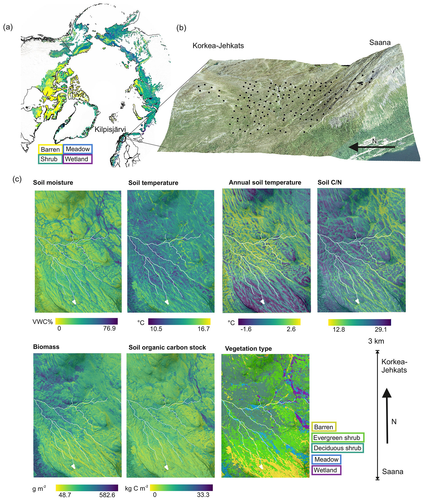
Figure 1The distribution of the main vegetation types across the Arctic tundra (Dinerstein et al., 2017; European Space Agency, 2017) and the location of our study area (a), the distribution of plots (b) and environmental conditions derived from statistical upscaling of in situ measurements (see Sect. 2.3.2) across the study area (c). Soil moisture and temperature represent mean daytime (08:00 to 20:00 EET) conditions from 1 July to 2 August, and annual soil temperature is an average within the entire year (July 2017–June 2018). Other variables represent growing season conditions and are considered static in this study. The aerial image is produced by the National Land Survey of Finland (2016).
2.2 Data
We measured GHG fluxes from 101 plots during the peak growing season (from now on, growing season). Environmental conditions explaining these GHG fluxes were measured at each plot. Most environmental variables had near-complete spatial coverage; missing data were filled using the environmental predictions (see Sect. 2.3.2, Table S1). We used additional in situ environmental data to upscale and visualize environmental conditions across the entire landscape (see Fig. 2): continuous soil moisture loggers (50 plots), continuous soil temperature loggers (139), soil samples for carbon and nitrogen stock and estimation (168), and vegetation classification data (5413). The full set of variables at a plot consisted of the plot for GHG flux measurements, and of a nearby complementing plot (max. 2 m distance) where we monitored soil moisture and temperature continuously and did a vegetation classification. The additional plot was separated from the GHG plot to avoid disturbance of the continuous recordings. The additional plot was carefully situated to similar vegetation and microtopographic conditions as the GHG plot. Soil samples were collected as close as possible to the GHG plot.
2.2.1 Chamber measurements
We measured GHG exchange using a static, non-steady-state non-flow-through system (Livingston and Hutchingson, 1995) composed of an acrylic chamber (20 cm diameter, 25 cm height). The chamber was placed on top of a collar and ventilated before each measurement. Prior to the measurements, we installed steel collars, which were 21 cm in diameter and 6–7 cm in height. Each collar was visited once during the growing season, and measurements were conducted between 10:00 and 17:00 EET. Although we did not have any temporal replicates, the spatial variation in our plots covered most of the temperature variation during the growing season. For more details, see Sect. S1.
For CO2 flux measurements, transparent and opaque chamber measurements were conducted during 1 and 27 July 2018. The chamber included a small fan, a CO2 probe GMP343, and an air humidity and temperature probe HMP75 (Vaisala, Finland). In the chamber, CO2 concentration, air temperature, and relative air humidity were recorded at 5 s intervals for 90 s. Photosynthetically active radiation was logged manually outside the chamber at 10 s intervals during the same period using a MQ-200 quantum sensor with a hand-held meter (Apogee Instruments, Inc, USA). MQ-200 measures photosynthetic photon flux density (PPFD) at a spectral range from 410 to 655 nm in µmol m−2 s−1. For more details of the equipment, see Happonen et al. (2022).
We progressively decreased the light intensity of net ecosystem exchange (NEE) measurements from ambient conditions to ca. 80 %, 50 % and 30 % PPFD by shading the chamber with layers of white mosquito net (replicate measurements per collar = 5–9). Ecosystem respiration (ER) was measured in dark conditions (0 PPFD), which were obtained by covering the chamber with a space blanket (replicates = 2–3). Before flux calculations, we discarded the first 0–5 s as well as the last 5 s of the measurements to remove potentially disturbed observations. Fluxes were calculated from the concentration change within the chamber headspace over time using linear regression (for performance statistics see Sect. S2).
We standardized NEE, gross primary productivity (GPP), and ER measurements conducted at different light and temperature conditions to allow across-plot comparison of the fluxes. We fitted light-response curves using a non-linear hierarchical Bayesian model with the plot as a random effect (Sect. S5). We used the Michaelis–Menten equation to model instantaneous NEE with plot-specific ER, maximum photosynthetic rate (GPPmax), and the half-saturation constant (K) as parameters using the same formula as in Williams et al. (2006) and Cahoon et al. (2012b). ER also had an exponential air temperature (T) response (for more details, see Happonen et al., 2022). We used this model to predict NEE at dark (0 PPFD, i.e., ER) and average light (600 PPFD) conditions and an air temperature of 20 ∘C at each plot; 20 ∘C was chosen as it represents a typical air temperature inside the chamber during flux measurements and 600 PPFD because it is widely used in tundra literature (Dagg and Lafleur, 2011; Shaver et al., 2007). We then subtracted ER from the NEE normalized to average light conditions to arrive at an estimate of normalized GPP. Negative values in NEE indicate a net sink of CO2 from the atmosphere to the ecosystems. GPP and ER are given as positive values.
We measured CH4 and N2O fluxes with an opaque chamber (0 PPFD). Measurements were conducted during 2 July and 2 August 2018. Five gas samples were taken within a 50 min enclosure time and transferred into 12 mL vials (Labco Exetainer, Labco Ltd.). The vials were pre-evacuated in the laboratory and filled with 25 mL of the sample in the field. Gas samples were analyzed at the University of Eastern Finland with a gas chromatograph (Agilent 7890B; Agilent Technologies, Santa Clara, CA, USA), equipped with an autosampler (Gilson Inc., Middleton, WI, USA), with thermal conductivity detector (TCD) for CO2, flame ionization detector (FID) for CH4, and an electron capture detector (ECD) for N2O. We calculated gas concentrations from sample peak areas relative to those derived from gas standards with known GHG concentrations (CO2: seven concentration levels ranging from 0–10 000 ppm; CH4: seven concentration levels ranging from 0–100 ppm; N2O: five concentration levels ranging from 0–5000 ppb). Fluxes were calculated from the concentration change within the chamber headspace over time using linear regression. Quality control was based on visual inspection and RMSE. We also verified that the RMSE was less than 3 ⋅ standard deviation of gas standards in a similar concentration range. Negative values in these fluxes represent net CH4 and N2O sinks from the atmosphere to the ecosystems.
2.2.2 Soil temperature and moisture data
Soil moisture and soil temperature were measured simultaneously during the flux measurements. We measured soil moisture with a time-domain reflectometry sensor (FieldScout TDR 300; Spectrum Technologies Inc., Plainfield, IL, USA; 0 to 7.5 cm depth). Soil temperature measurements conducted at the same time as CO2 flux measurements were taken with a thermometer (TD 11 thermometer; VWR International bvba; Leuven, Germany; 6.0 to 7.5 cm depth). Soil temperature measurements (TM-80N measure and ATT-50 sensor) conducted at the same time as CH4 and N2O flux measurements were taken with a thermometer in the uppermost 10 cm. We refer to these variables as soil moisture and soil temperature throughout the text.
Temperature loggers (Thermochron iButton DS1921G and DS1922L, San Jose, CA, USA, and TMS-4; TOMST s.r.o., Prague, Czech Republic) monitored temperatures at 7.5 and 6.5 cm (iButton and TMS-4, respectively) below ground at 0.25–4 h intervals (Sect. S3). We calculated a variable describing average soil temperature conditions during the previous 12 months by averaging the measurements from the study design (n=138) from July 2017 to June 2018. We refer to this variable as annual soil temperature. In addition to temperature, the TMS-4 loggers also monitored soil moisture (raw time-domain transmission data between 1 and 4095) to a depth of ca. 14 cm (Wild et al., 2019). The raw time-domain transmission data were transformed into volumetric water content (VWC%) (Tyystjärvi et al., 2022).
These continuous soil moisture and temperature data were used to upscale soil microclimatic conditions at 2 h time steps during daytime (08:00 to 20:00) and from 1 July to 2 August. This period was chosen because the GHG fluxes were measured during this period, and we did not want to extrapolate outside our main measurement campaign. Moreover, this period represents the peak growing season of this region.
2.2.3 Vegetation data
We took images from CH4 and N2O collars on the measurement day and used them to classify the dominant vegetation to five distinct classes, following the Circumpolar Arctic Vegetation Map physiognomic classification system (Walker et al., 2005) with minor modifications (Fig. 1). We used the following classes: barren (<10 % vegetation cover), evergreen shrub, deciduous shrub, meadow (graminoids and forbs), and wetlands. The sample sizes were not even between vegetation types; rather they roughly represent the spatial coverage of each vegetation type (8 observations of barren, 38 of evergreen shrub, 14 of deciduous shrub, 26 of meadow, and 15 of wetland). We utilized a larger dataset of 5413 vegetation descriptions in total estimated in the field and from aerial imagery from the study design to create the vegetation type map (for more details, see Sect. S4.1). We collected biomass samples from above-ground vascular plants using the clip-harvest method during late peak season, between 17 July and 10 August. Samples were collected within the chamber collars and were oven-dried at 70 ∘C for 48 h and weighed after drying. We refer to this variable as biomass (g dry weight m−2).
2.2.4 Soil sampling and analyses
We measured the thickness of the organic and mineral soil layers using a metal probe reaching up to 80 cm depth. We collected soil samples (ca. 1 dL) from the organic and mineral layers using metal soil core cylinders (4–6 cm Ø, 5–7 cm height) during August in 2016–2018. The organic samples were collected from the top soil and mineral samples directly below the organic layer, which was on average 6.6 cm deep. Large roots were excluded from the samples. The soil samples were freeze-dried and analyzed in the Laboratory of Geosciences and Geography and Laboratory of Forest Sciences (University of Helsinki). Bulk density (kg m−3) was estimated by dividing the dry weight by the sample volume. Soil organic layer pH was analyzed following ISO standard 10390. Total carbon and nitrogen content (C%, N%) analyses were done using Vario Elementar Micro cube and Vario Elementar Max analyzer (Elementar Analysensysteme GmbH, Germany). Prior to CN% analysis, mineral samples were sieved through a 2 mm plastic sieve. Organic samples were homogenized by hammering the material into smaller pieces.
Soils in this landscape are acidic and likely have a minimal amount of carbonates; consequently, we assumed C% to equal organic C%. Soil organic carbon and nitrogen stocks were calculated for the entire soil horizon up to 80 cm (in 95 % of plots soil depth was less than that). Some plots lacked CN% data (30 % of the plots), and therefore we used soil organic matter content estimated with the loss-on-ignition method according to SFS (1990) to derive C%. We utilized a similar stock calculation framework using the bulk density, layer depth, and C% and N% data as in Kemppinen et al. (2021) except we used average bulk density and mineral C% estimates in each vegetation type in case that information was missing in stock calculation.
Soil samples for dissolved organic carbon concentration analyses in dry soil were collected between the 5 and 14 July 2018. After the collection, samples were stored at 4 ∘C and then dried at 60 ∘C for at least 5 d. Extraction of dissolved organic carbon was done using pure water extractions with 0.5 to 3 g of dried soil added to 40 mL of water following the WEOC protocol from Hensgens et al. (2021). Extracts were immediately filtered (0.7 µm) using glass fiber filters, diluted, acidified to remove inorganic carbon, and measured on a Shimadzu TOC V-CPN analyzer set on the nonpurgeable organic carbon mode. We refer to this variable as dissolved organic carbon.
2.2.5 Remotely sensed data
Remotely sensed optical and light detection and ranging-based (lidar) data describing topographic, vegetation, snow, and surficial deposit conditions were used for upscaling the in situ measured environmental variables (Fig. 2, Sect. S4 and Fig. S1 in the Supplement).
2.3 Statistical analyses
We investigated the dependencies of GPP, ER, NEE, CH4 flux, and N2O flux on environmental variables using statistical analyses which included analysis of variance (ANOVA) and machine learning modeling and prediction. We developed machine learning models, in which we (1) upscaled environmental data (annual soil temperature, soil temperature, soil moisture, soil , soil organic carbon stock, vegetation type, biomass) using remotely sensed variables as predictors; (2) modeled GHG fluxes using the environmental data as predictors, and (3) upscaled GHG fluxes using the upscaled environmental data maps at a 2 m spatial resolution across the landscape (Fig. 2). This two-step upscaling approach enabled us to focus on the relationships between GHG fluxes with their physical and ecological, in situ measured environmental controls instead of the remotely sensed data that are proxies by nature. We ran all analyses in the R statistical programming environment (R Core Team, 2020; version 4.0.3). We used the ArcGIS Pro 3.0.3 software to visualize spatial data (ESRI, 2022).
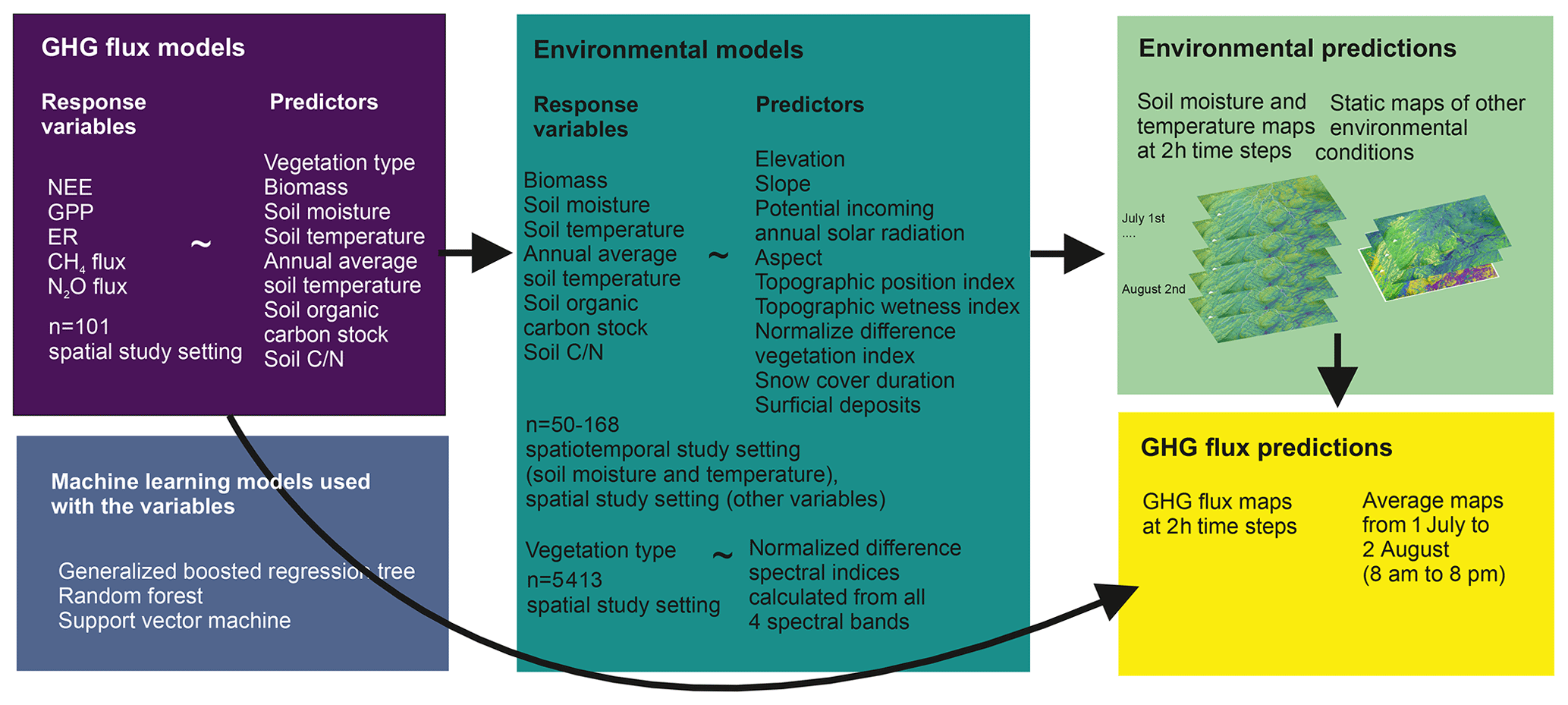
Figure 2The upscaling framework used in this study. We first linked GHG fluxes to the in situ environmental drivers using machine learning models. Then we trained three machine learning models to upscale environmental conditions across the landscape using remote sensing data. Then we used the GHG flux models and environmental predictions to upscale GHG fluxes across the landscape throughout the entire growing season.
2.3.1 Analysis of variance (ANOVA)
We used one-way ANOVAs to test for vegetation type differences in environmental conditions and GHG fluxes, and we tested significance using multiple comparisons with Tukey's honest significant difference test (p<0.05). CH4 flux, soil moisture, soil organic carbon and nitrogen stock, and biomass were not normally distributed. Thus we used Kruskal–Wallis test instead of ANOVA.
2.3.2 Machine learning models
We modeled our response variables using three machine-learning methods (generalized boosted regression models, GBM; random forest, RF; and support vector machine regression, SVM), all of which have been widely used in flux upscaling studies (see, e.g., Natali et al., 2019; Peltola et al., 2019; Tramontana et al., 2016). These three approaches are non-parametric and can handle linear and non-linear relationships and different data distributions. We chose RFs and GBMs because they utilize several decision trees in an ensemble model framework and thus avoid overfitting, have high accuracy, are highly adaptable, and are not significantly impacted by outliers. We chose SVMs because they are good at generalizing the relationships in the data. Based on these models, we visualized the partial dependence plots characterizing the relationships between the response and predictor variables while accounting for the average effect of the other predictors in the model using the pdp package (Greenwell, 2017). Further, we calculated variable importance using the vip package (Greenwell and Boehmke, 2020). Variable importance scores were estimated by randomly permuting the values of the predictor in the training data and exploring how this influenced model performance based on the adjusted R2 values, with the idea that random permutation would decrease model performance (Breiman, 2001). We used 100 simulations to calculate 100 importance scores which were averaged. A standard deviation across these scores was used as an uncertainty estimate, together with the differences in average importance across models. For more details, see Sect. S5.
We used 10 topography, snow, vegetation, and surficial deposits variables to construct landscape-wide predictors matching the in situ environmental conditions that we used to model the GHG flux values. These variables were the following: elevation, topographic wetness index, topographic position index at 5 and 30 m radii, aspect, slope, potential incoming solar radiation, normalized difference vegetation index, snow cover duration, and surface deposits. Soil organic carbon stocks, soil , biomass, and annual soil temperature models were calibrated only once, and a single prediction was made to the landscape. Soil temperatures and moisture vary throughout the growing season; thus, we calibrated each model at each time step and created 231 predictions over the study period (every 2 h between 08:00 and 20:00 from 1 July until 2 August). For each variable, an ensemble prediction was produced by calculating a median prediction over the three predictions from the different modeling methods.
We examined the relationship between the five primary response variables (GPP, ER, NEE, CH4 flux, N2O flux) and environmental predictors that describe (i) soil resources and conditions (soil moisture, soil , soil pH), which are relevant to, for example, the growth of organisms (Nobrega and Grogan, 2008; Happonen et al., 2022); (ii) soil C and N stocks and dissolved organic carbon, which are one of the main sources for the GHG emissions (Bradley-Cook and Virginia, 2018); (iii) soil temperatures, which regulate enzymatic processes (St Pierre et al., 2019; Mauritz et al., 2017); and (iv) biomass and vegetation type, which describe resource-use strategies, carbon inputs to soils and plant photosynthetic capacity and integrate multiple environmental properties into one variable (Magnani et al., 2022). We excluded soil pH and soil nitrogen stock from modeling analyses due to high correlations (Pearson's r>0.7) with soil moisture and soil organic carbon stock, respectively. Further, dissolved organic carbon was excluded due to its low importance in all the models. We did not use air temperature as a predictor as we already controlled for it in CO2 fluxes in the light-response model, and we assumed that soil microbes regulating CH4 and N2O cycling are most importantly driven by soil temperatures (Kuhn et al., 2021). The final predictors for our models were soil moisture, soil temperature, annual soil temperature, soil organic carbon stock, soil , biomass, and vegetation type. The machine learning parameters tuned for each model can be found from Sect. S5.
We used the machine learning models to predict GHG fluxes across the landscape for each 2 h time step from 1 July until 2 August. Similar to the environmental predictions, an ensemble prediction was produced by calculating a median prediction over the three predictions from the different modeling methods. As our focus was on understanding the spatial patterns in the mean growing season fluxes, we averaged GHG flux predictions over the study period. However, a visualization of the predicted mean daily patterns in soil moisture and temperatures and the consequent GHG fluxes is provided in the Supplement (Fig. S2).
To compare the magnitude of all three important GHGs, namely CO2, CH4, and N2O, we calculated the radiative forcing strength of the three GHGs over a 100-year period from our measurements and ensemble predictions. We used the global warming potential (GWP; 27 for CH4 and 273 for N2O, IPCC, 2021) and sustained GWP (45 for CH4 and 270 for N2O, Neubauer and Megonigal, 2015), which are, to our knowledge, the best and most widely used approaches that exist to compare flux magnitudes. We acknowledge that these approaches are designed to quantify an effect of a change in emission to the radiative forcing and are thus not fully suitable to be used to quantify the climatic effect of natural continuous fluxes in our study (Mathijssen et al., 2022; Frolking et al., 2006).
For all of our models, we used a leave-one-plot-out cross-validation scheme in which each plot was iteratively left out from the dataset, and the remaining data were used to predict fluxes for the excluded plot to assess the predictive performance of the models (Bodesheim et al., 2018). Estimates of bias were calculated as an average of the absolute error (MAE) between prediction and actual observation. Coefficient of determination (R2) was used to determine the strength of the linear relationship between the observed and predicted fluxes.
The root mean squared error (RMSE) was used to estimate the model error. The same evaluation metrics were also calculated based on the prediction to the full model training data to represent model fit (Virkkala et al., 2021); see Table S3, which presents these for the individual models. Uncertainty in GHG flux predictions was derived by bootstrapping (fractional resampling with replacement based on vegetation type classes). We subset the model training data into 30 different datasets, all of which had the same number of observations as the original data itself. These 30 datasets were then used to produce 30 individual predictions for a subset of the times with all three machine learning models and their ensemble for each response variable (Sect. S5). The uncertainty estimates represent how different distributions of the input data as well as model parameters influence the upscaled flux maps.
3.1 Environmental conditions and GHG fluxes across vegetation types
We observed large variability in GHG fluxes and environmental conditions within and across vegetation types (Fig. 3, Table S2). The variability within the vegetation types differed depending on the flux and environmental variable considered (e.g., meadow class had large variability in GPP and evergreen shrub class in soil ). Frequently, wetlands differed clearly from the other vegetation types. While wetlands had high CH4 emissions, all the other vegetation types with significantly lower soil moisture showed CH4 uptake. Meadows were a significantly larger net CO2 sink than evergreen shrub sites, while other vegetation types had intermediate NEE values. The N2O fluxes were low from all vegetation types and varied between small sinks and small sources.
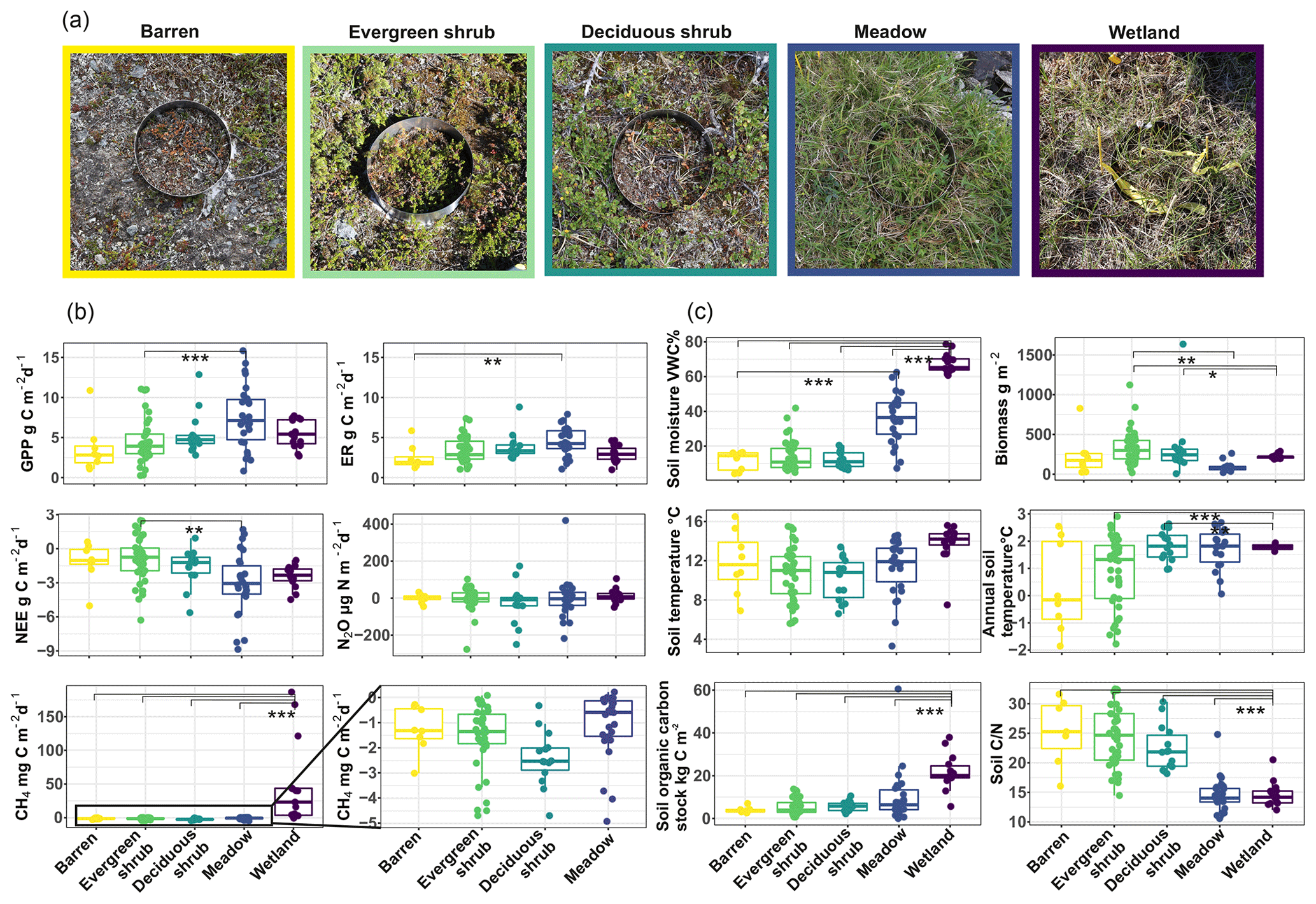
Figure 3The vegetation types considered in this study (a), the distribution of GHG fluxes (b), and environmental conditions (c) across the vegetation types. Lines represent Tukey's test results (* = p≤0.05, = p≤0.01, = p≤0.001). The box corresponds to the 25th and 75th percentiles, and the line within the box represents the median. The lines denote the 1.5 IQR of the lower and higher quartile, where IQR is the inter-quartile range, or distance between the first and third quartiles.
3.2 The performance of environmental and greenhouse gas flux models
The predictive performance of the ensemble environmental variable models was rather high but varied depending on the variable (R2: 0.09–0.71; Fig. S3). The predictive performance of the GHG models was for most variables lower (R2: 0.00–0.52), with N2O flux models being close to random and GPP models performing the best (Fig. 4). Model fit was significantly higher than predictive performance for all the fluxes (Table S3). The scatterplots of observed and cross-validation-based predicted GHG fluxes suggest that the highest flux estimates are often predicted most poorly, but the mean fluxes in each vegetation type were predicted accurately, as expected.
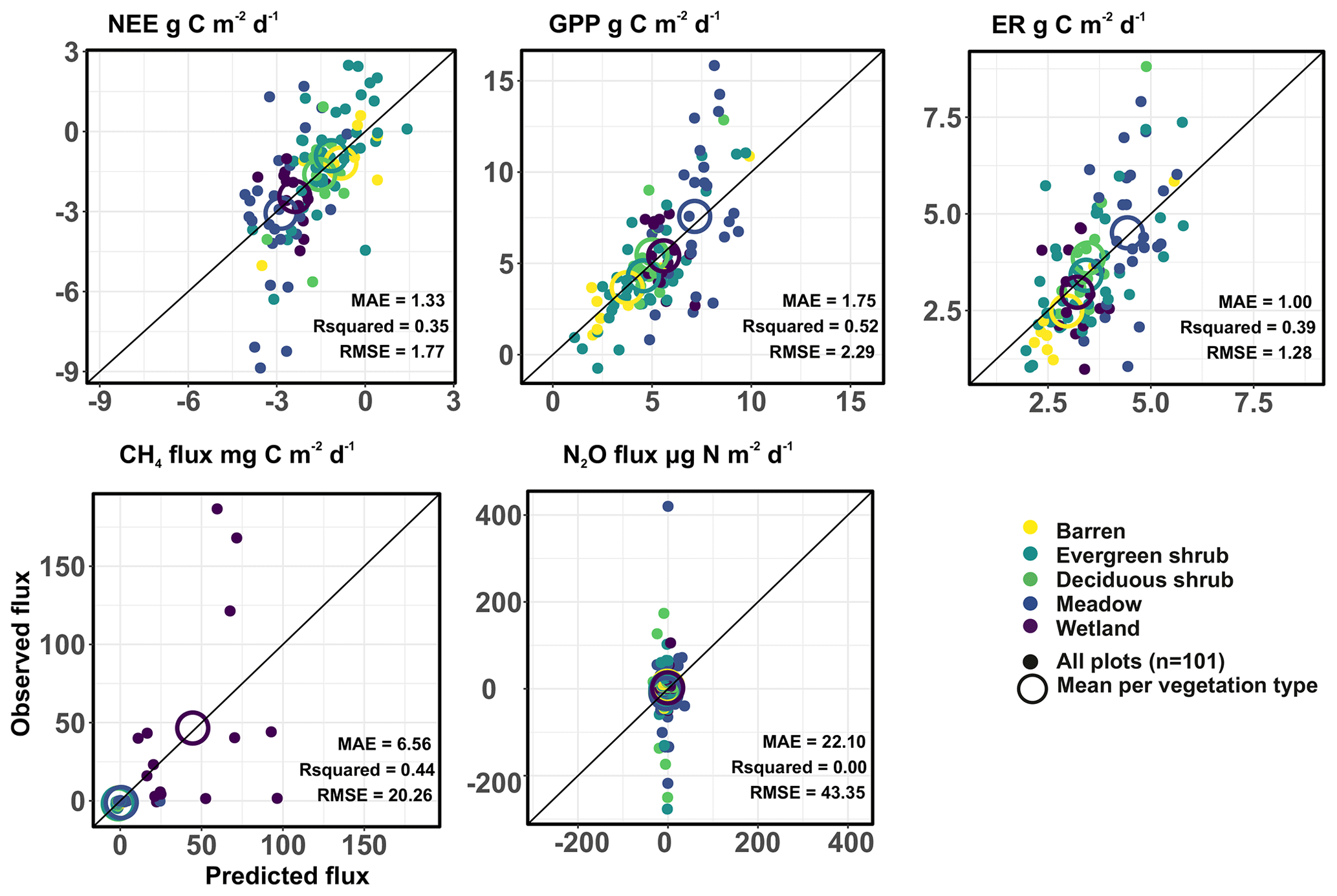
Figure 4The correlation between observed and predicted values based on the ensemble model predictions (i.e., median of the three machine learning model outputs). Model predictive performance is described with mean absolute error (MAE), R2 (R squared), and RMSE (root mean square error).
3.3 Drivers of greenhouse gas fluxes
The most important controlling variables and the response shapes differed depending on the GHG flux (Figs. 5, 6 and S4) and sometimes also depending on the machine learning model type applied. CO2 fluxes were driven by annual average soil temperature, biomass, and vegetation type. In addition, soil organic carbon stocks were an important predictor for ER. Soil moisture and vegetation type were the most important predictors for CH4 fluxes, and soil and soil moisture for N2O fluxes. In general, warmer and wetter conditions increased net emissions of CH4 and N2O and net uptake of CO2. Some fluxes were further positively correlated with soil organic carbon stocks (ER, CH4 flux) and negatively with soil (GPP, ER, N2O). The importance for variables explaining the N2O flux is low because the model predictive performance is close to random.
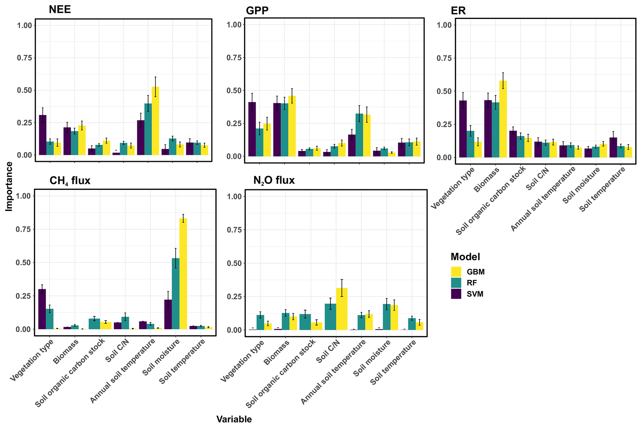
Figure 5The variable importance of the environmental variables used to predict GHG fluxes. The models were generalized boosted regression models (GBM), random forest (RF), and support vector machine regression (SVM).
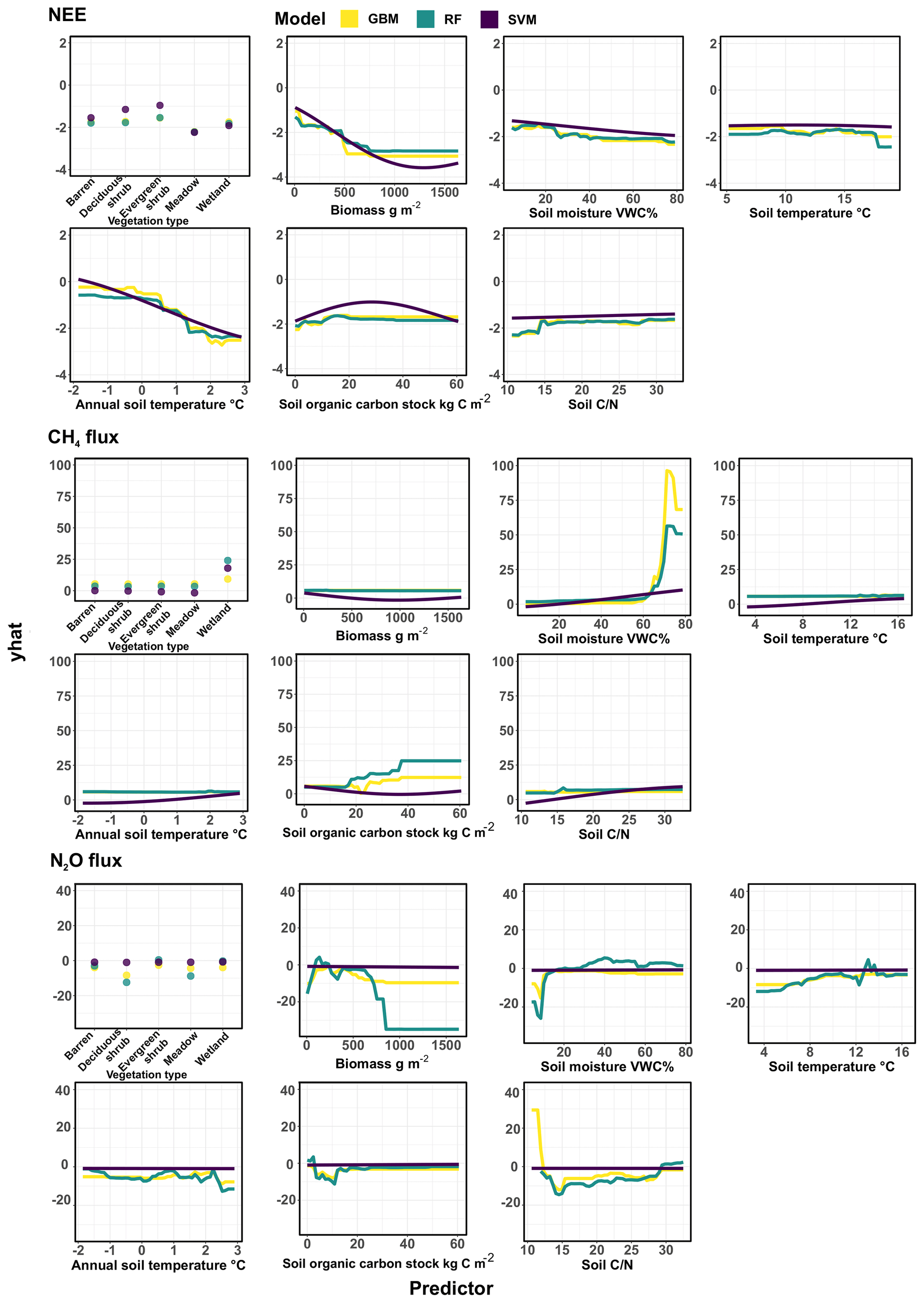
Figure 6Partial dependence plots showing the relationships between GHG fluxes and environmental conditions across the three models (generalized boosted regression models, GBM; random forest, RF; and support vector machine regression, SVM). The y axis of the plot (yhat) represents the marginal effect of the predictor on the response and should not be directly compared with observed or predicted values, rather the shape and direction of the response instead. RFs and GBMs are based on decision trees, where trees are split based on a certain threshold in the data, which can be seen as thresholds in the partial dependence plots as well. SVMs map the data into a high-dimensional space where a hyperplane is fit to separate them, creating smoother response shapes. Partial dependence plots for GPP and ER are found in Fig. S4.
3.4 Spatial patterns and contributions in greenhouse gas flux predictions
The model predictions show large spatial variability in GHG fluxes across the landscape (Figs. 7, S5). Net CO2 uptake as well as GPP and ER were highest in the warm and productive meadow locations of the valley, whereas CH4 and N2O fluxes were highest in the eastern parts of the landscape that is dominated by wetlands. The prediction suggests small but widespread net CH4 uptake across the entire upland region. CO2 was the most important flux contributing to the net GHG sink (Fig. 8). Mean fluxes calculated based on the upscaled flux maps differ from the in situ based ones, particularly for wetland CH4 emissions (Figs. 8, S6).
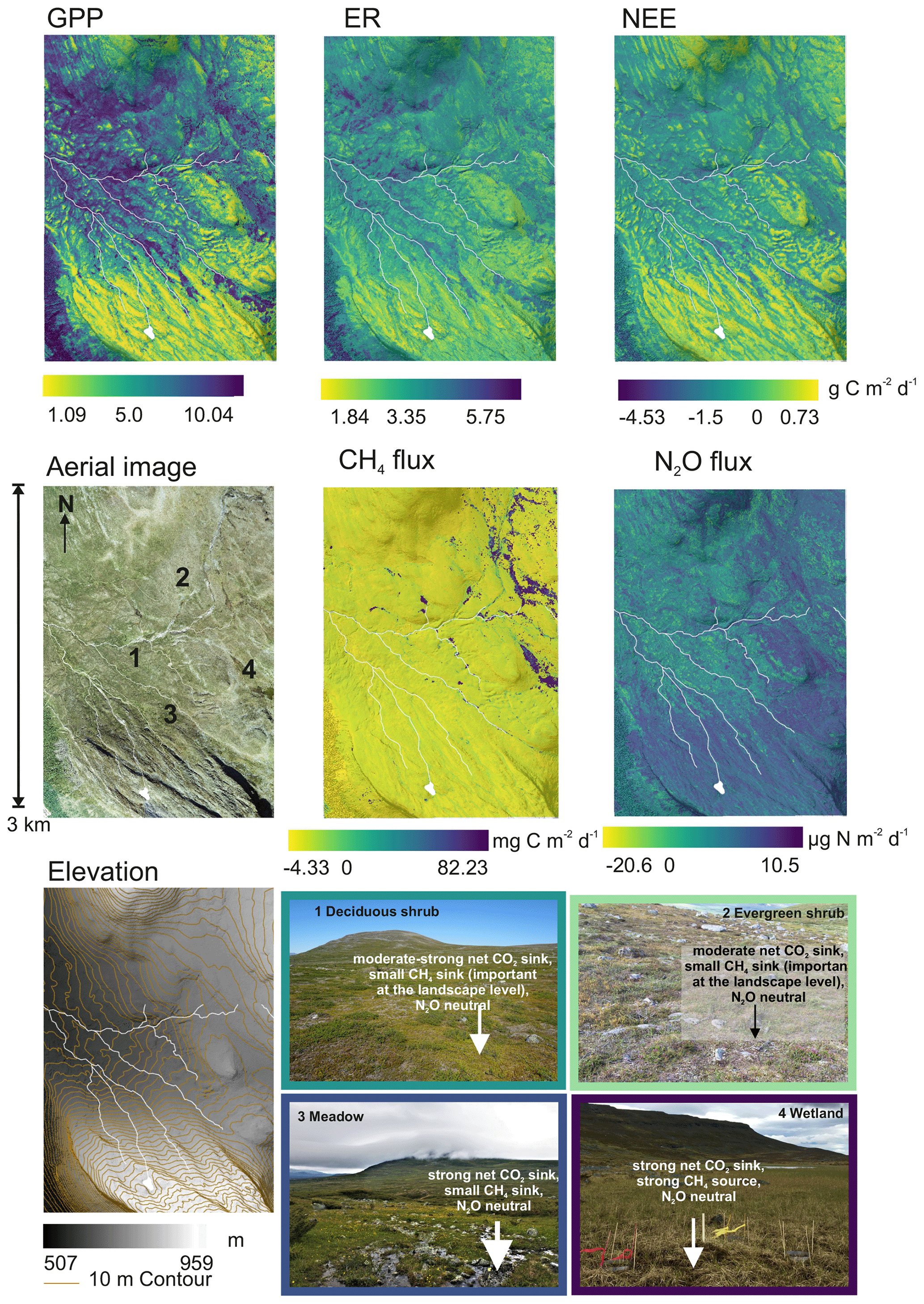
Figure 7Ensemble predictions of growing season GHG fluxes, averaged over 1 July to 2 August (only daytime variability between 08:00 and 20:00 considered) and photographs summarizing the main sink–source patterns in the landscape. Note that the southwestern corner of the study design has mountain birch forest for which we did not have any data; we did not have measurements from the northeastern corner either.
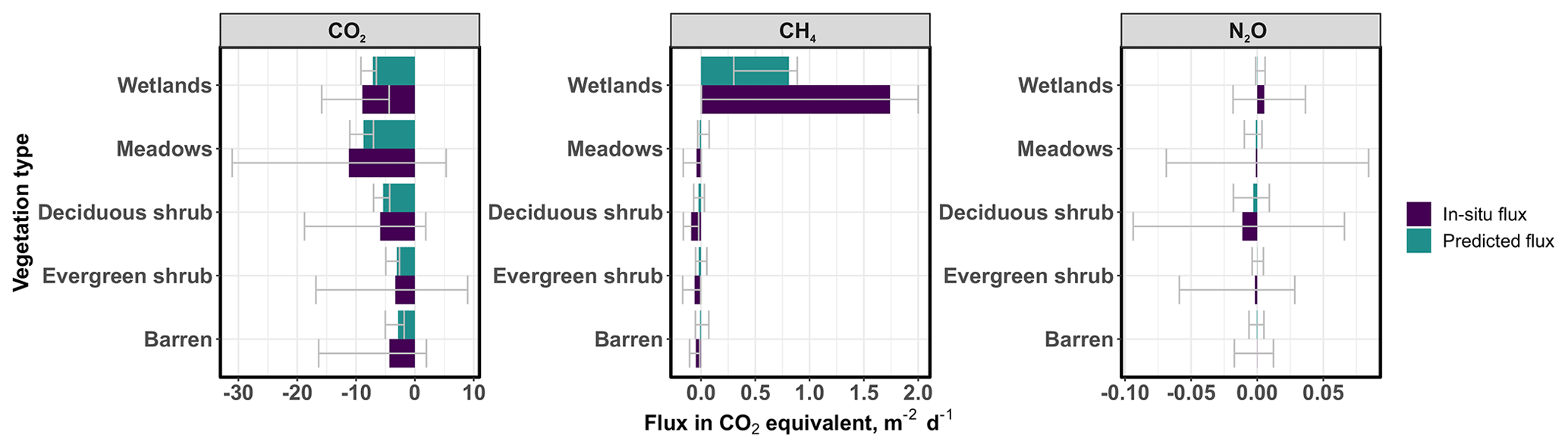
Figure 8Growing season mean and percentile (0.025 and 0.975) GHG fluxes in CO2 equivalents based on in situ data and upscaled flux predictions, averaged across the entire study period (only daytime variability between 08:00 and 20:00 considered) and across vegetation types. Note that the scale for the x axis is different for each gas species, and that the uncertainties in in situ versus predicted mean fluxes cannot be directly compared with each other. The uncertainty in in situ wetland CH4 continues up to 6.7 but was cropped for visualization purposes. The same graph using the sustained GWP approach can be found in the Supplement Fig. 6 and demonstrates the potentially larger role of CH4 fluxes over a 100-year horizon in this landscape.
4.1 CO2 fluxes driven by both biotic and abiotic variables
Our results show the importance of several environmental variables for CO2 fluxes, demonstrating the strong dependence of GPP and ER on a wide range of soil microclimatological, hydrological, soil biogeochemical, and ecological processes (Sørensen et al., 2019; Dagg and Lafleur, 2011; Nobrega and Grogan, 2008; Cahoon et al., 2016). Overall, the relationships with environmental conditions and GPP and ER were rather similar. Biomass was a more important predictor than vegetation type for all the CO2 fluxes, indicating that the quantity of plant material producing and emitting carbon was potentially more important than the different types of plants associated with CO2 cycling in this study setting (Happonen et al., 2022). The high importance of plant-related variables (e.g., leaf area index) as drivers of spatial variability in CO2 fluxes has been previously found in other tundra landscapes (Marushchak et al., 2013, and references therein).
Our models also show that annual soil temperatures have a different and stronger relationship with CO2 fluxes than instantaneous growing season soil temperatures, and these two soil temperature variables are indeed not strongly correlated with each other in this study design. This is because annual soil temperatures are driven by winter soil temperatures, which increase with thicker snow cover that is found particularly in the valley and in microtopographic depressions, which are colder in the summer. Moreover, annual soil temperatures integrate many other environmental conditions from the entire year: they reflect growing season length and temperature conditions, regulate C and N availability, and control vegetation and microbial community composition and functioning over long timescales. These conditions have been shown to be important drivers of CO2 fluxes across a range of Arctic sites (Zona et al., 2022; Lund et al., 2010). Similar to these previous studies, we observed that plots with warmer annual soil conditions have larger growing season GPP and ER fluxes and stronger net uptake. Our results also show other logical relationships between environmental conditions and CO2 fluxes. For example, GPP and ER increased with soil moisture (Nobrega and Grogan, 2008). However, at around 50 %–60 % VWC this relationship plateaued and turned negative. This was likely due to the lack of oxygen for plant roots restricting growth of non-aerenchymous plants. Furthermore, the lack of oxygen allows only anoxic metabolic pathways for microbes, such as CH4 production in methanogenesis, where CO2 production is low (Bridgham et al., 2013). Further, soil organic carbon stock was an important predictor for ER, but not so much for GPP. This was likely related to the higher soil carbon contents boosting decomposition (Schlesinger and Andrews, 2000).
4.2 Small but consistent net CH4 uptake mostly driven by soil moisture
Net CH4 flux was strongly controlled by soil moisture due to its effect on regulating the anoxic and oxic soil conditions, and therefore CH4 production (methanogenesis) and CH4 consumption (CH4 oxidation, or methanotrophy) (Kelsey et al., 2016; Christensen et al., 1996; Treat et al., 2018b). Our results demonstrate that the rate of CH4 emissions increases sharply in water-logged soil conditions, i.e., at soil moisture levels of >60 VWC% (Vainio et al., 2021). In drier conditions (VWC < 60 %), soils contain more oxygen, which prevents CH4 production and increases net CH4 uptake. This result supports findings from recent studies that show that drier upland tundra areas can be habitats for methane-oxidizing bacteria, which can use CH4 from the atmosphere as their main energy source, transforming these environments to net CH4 sinks (Christiansen et al., 2015; Juncher Jørgensen et al., 2015; Lau et al., 2015; Emmerton et al., 2014; Wagner et al., 2019; St Pierre et al., 2019; Voigt et al., 2023). Given the large area of the Arctic, even minor fluxes such as those observed here for CH4 uptake can be of global importance. This CH4 uptake can strengthen the GHG sink of the Arctic and prevent CH4 from entering the atmosphere.
Our results show that net CH4 uptake increases not only in drier conditions but also in soils with low and soil organic carbon stocks. This is likely due to microbes needing and getting C and energy from the atmosphere due to limited soil C supply (Lau et al., 2015; Juutinen et al., 2022), and the capability of methanotrophs to effectively compete against classical heterotrophs dependent on larger organic macromolecules in these environments. The models did not clearly identify a particular vegetation type controlling net CH4 uptake; however some individual models demonstrated deciduous shrubs and meadows to be more closely related to net CH4 uptake (Larmola et al., 2010). Overall, our results indicate that net CH4 uptake potential is present in any kind of upland tundra vegetation type (Fig. S7) as long as the abiotic conditions for microbes responsible for atmospheric CH4 consumption are favorable.
Methane fluxes had a rather uniform distribution across the mineral upland regions (i.e., small but consistent net uptake). High CH4 emissions were located in wetland regions dominated by high soil organic carbon stocks and moisture levels. Our observations demonstrated similar or even higher net CH4 uptake than previous studies. For example, dry tundra was CH4 neutral in a recent Arctic–boreal CH4 flux synthesis (mean = 3.83, median = −0.01 mg CH4 m−2 d−1), primarily based on growing season daytime fluxes (Kuhn et al., 2021), whereas our study showed higher uptake rates for the non-wetland plots (mean = −2.05, median = −1.81 mg CH4 m−2 d−1). However, studies focusing on individual sites have recorded similar CH4 flux magnitudes as observed here (Emmerton et al., 2014; Lau et al., 2015), but to the best of our knowledge, such extensive spatial patterns in CH4 flux uptake using fine spatial resolution models as presented here have not been published so far.
4.3 N2O fluxes remain neglectable and unpredictable
We observed moderate and to a large extent unpredictable variability in N2O fluxes in this landscape. The differences in average fluxes between the vegetation types were small. Based on our observations, most vegetation types were on average N2O sinks or neutral, but deciduous and evergreen shrubs and meadows had some variability from moderate N2O sinks (up to −200 µg N m−2 d−1) to moderate N2O sources (up to 400 µg N m−2 d−1). Overall, our average N2O fluxes were close to zero and thus low in the light of the recent review (Voigt et al., 2020), which demonstrated that vegetated soils in permafrost regions are often small but evident sources of N2O during the growing season (∼ 30 µg N m−2 d−1) and that barren or sparsely vegetated soils serve as substantial sources of N2O (∼ 455 µg N m−2 d−1). The relatively small N2O fluxes observed here can be explained by the nitrogen-limited nature of the studied soils and the strong competition between plants and microbes for nutrients: with shallow soils and low stocks of soil organic nitrogen, nitrogen release in labile forms by mineralization remains low (Voigt et al., 2020). Most of the data in the synthesis came from ecosystems that are not as much nitrogen-limited as our site (e.g., peatlands, grasslands).
We were unable to explain the patterns in N2O fluxes with the predictors used here. This was likely related to the relatively low variability in N2O fluxes in most of the plots in general and the complexity of the soil microbial N cycle, where N2O is produced (nitrification, denitrification, DNRA) and consumed (denitrification) by multiple co-occurring processes, differently regulated by environmental variables (Butterbach-Bahl et al., 2013). Nevertheless, the most important driver of N2O flux was soil , and the models suggested that lower ratios were linked to higher net N2O emissions. This is expected as the excess soil N in soils with low C : N ratio allows more rapid N mineralization, nitrification, and denitrification as compared to microbial immobilization, which accelerates N2O emissions (Klemedtsson et al., 2005; Liimatainen et al., 2018). Further, N2O emissions were highest in the wetlands, similar to Ma et al. (2007), who explained this by high ammonia or nitrate levels boosting N2O production. The uppermost soil layers were also likely not fully saturated by water at the time of the wetland measurements, which can induce higher N2O emissions in oxic but still moist conditions, which allow aerobic nitrification and anaerobic denitrification to co-occur (Voigt et al., 2020; Takakai et al., 2008). In contrast to C fluxes, vegetation type did not play an important role for N2O fluxes. This might be related to our study having no measurements in the previously observed, clear N2O flux hotspots located in barren permafrost peatlands, such as peat plateaus or palsas, with thick organic layers and high inorganic N content (Repo et al., 2009; Voigt et al., 2017a).
4.4 The sub-Arctic tundra landscape is a strong growing season GHG sink
Our results demonstrate a high level of spatial heterogeneity in the growing season GHG fluxes across the landscape, with areas acting as both net CO2, CH4, and N2O sinks and sources in some parts of it. Areas acting as GHG sinks covered most of the landscape (CO2: 91 %, CH4: 87 %, N2O: 73 %; 62 % of the area was a sink for all three GHGs). We observed clear differences in flux magnitudes driven by key environmental conditions. Moist and carbon- and nitrogen-rich meadows and deciduous shrub heaths were strong GHG sinks. Wet sedge-dominated fens were GHG sinks with CH4 emissions being compensated by net CO2 uptake. Barren lands and evergreen shrubs were more resource-limited and closer to GHG neutral. These results are interesting in the light of the shrubification patterns observed across the entire Arctic (Myers-Smith et al., 2011; Parker et al., 2015; Vowles and Björk, 2018) and indicate that deciduous or evergreen shrub expansion may increase or decrease the growing season GHG sink. If shrubs expand to meadows, the GHG sink may decrease, whereas if they invade barren areas, the GHG sink may increase. However, our results did not quantify this change over time or cover the entire year to confirm the net annual effect.
Our results indicate that this heterogeneous Arctic landscape was a cumulative net GHG sink during the measurement period during daytime (08:00 to 20:00) in July 2018. The July budget for CO2 was −4.7 g C m−2 per month, for CH4 0.73 mg C m−2 per month, and for N2O −10.0 µg N m−2 per month. The CO2 sink is relatively small, likely due to the high cover of patchy and sparsely vegetated areas that were often CO2 sources. This small sink value is an overestimation of the sink activity considering the whole course of the day as we did not have measurements from the nighttime and did thus not upscale fluxes in nighttime conditions when ecosystems are net CO2 sources due to the lack of light required for photosynthesis. It also overestimates the importance of CO2 as a radiative forcing agent, since ecosystem CO2 production during autumn and winter contributes substantially to the annual C balance (Celis et al., 2017; Commane et al., 2017), thereby reducing the CO2 sink strength on an annual basis. Further, CH4 uptake might continue even in rather cold conditions as long as soils remain dry and unfrozen (Emmerton et al., 2014). Nevertheless, our results demonstrate that net CO2 uptake plays the most important role for the net growing season GHG budget. CH4 emissions from wetlands are almost balanced by the net CH4 uptake of other ecosystems. The role of N2O fluxes for the net GHG budget across the entire landscape is negligible for the growing season.
4.5 Methodological considerations in GHG flux modeling
Our study creates new understanding about high-resolution upscaling of GHG fluxes by incorporating more chamber measurements, predictors, models, and environmental gradients compared to earlier efforts (Fox et al., 2008; Dinsmore et al., 2017; Räsänen et al., 2021; Juutinen et al., 2022; Vainio et al., 2021). For example, we included chamber measurements from 101 plots, whereas earlier local-scale upscaling studies have usually had circa 30 plots. Further, we included seven different environmental predictors, while other studies have often used only one or two, focusing on predictors describing vegetation type or soil moisture. Finally, we studied a tundra landscape that consists of almost all the main vegetation types of the entire Arctic, whereas earlier studies have investigated a narrower range of vegetation conditions, with a focus on wet ecosystems. However, at the same time, our models showed some signs of overfitting as demonstrated by the high model fit performance statistics and the mismatch between model fit and predictive performance statistics (Sect. S5.3 in the Supplement). This is a common issue in upscaling (Kemppinen et al., 2018) and could indicate that the models have potentially learned to fit some noise or specific patterns unique to the training set instead of broadly generalizable relationships. Nevertheless, the relationships we observed were logical and comparable to those observed in other studies – both based on spatial and time series study designs (e.g., positive soil moisture–CH4 flux or soil temperature–ER relationships; Euskirchen et al., 2014; Davidson et al., 2016; Zona et al., 2023). Moreover, our study is based on a dataset focusing on spatial variation in GHG fluxes and correlations between variables. Therefore, the dataset should not directly be used to infer causal relationships or estimates of flux change over time (Damgaard, 2019), and we advise caution when extrapolating these results to areas outside our study domain or different time periods.
Our study showed that using means of in situ GHG fluxes in each vegetation class to derive a landscape-level GHG budget might produce significantly different results compared to the upscaled budget. This was apparent particularly for CH4 fluxes, where the in situ based average wetland CH4 emission was more than 2 times larger CH4 compared to the upscaled one. This mismatch is likely explained by the heterogeneity of environmental conditions and CH4 fluxes within the wetland class that the chamber measurements alone could not cover (Fig. S7). A multivariate machine learning modeling approach with variables describing not only vegetation type but also soil moisture and other conditions was likely able to characterize the resulting CH4 flux variability in a more representative way. For example, our soil moisture maps showed high variation in soil moisture between ca. 50 VWC% and 70 VWC% within the wetland areas, and high CH4 emissions were observed only in areas with 60 VWC%. Overall, this result suggests that simple land cover-based upscaling efforts might lead to biased budget estimates, especially when spatial variability within land cover types is high, emphasizing the need for multivariate modeling in flux upscaling.
The performance of our models varied from good (GPP, CH4 flux), moderate (ER and NEE), to low (N2O). CH4 fluxes – both sources and sinks – were accurately modeled, providing important support for future studies predicting not only the large CH4 emissions but also the previously unquantified CH4 uptake in Arctic landscapes. The lower predictive performance of the models for other GHG fluxes might be explained by the dynamic nature of fluxes not being represented in our spatial study design with no temporal chamber replicates in the plots, our models lacking important predictors, or our model structure not being ideal. The performance of the models could potentially be improved by describing plant functional composition using plant traits (Happonen et al., 2022) and including more detailed information about soil nutrients (e.g., soil nitrate or ammonium concentrations as soil captures only very roughly how much N is available) or microbial communities (e.g., communities or genes associated with nitrification or methanogenesis or methanotrophy; Pessi et al., 2022).
Rainfall events are another source of uncertainty in our upscaling because they might increase soil moisture levels and activate processes related to methanogenesis, photosynthesis, and respiration as well as nitrogen cycling. While our soil moisture predictions should capture these variations in soil wetness, we only made measurements once per plot under clear conditions and do not have information about how GHG fluxes might respond to rainfall events. We might thus underestimate some of the instantaneous and longer-term changes in GHG fluxes during and after rain (see Sect. S1 and Fig. S10 for details).
We chose to use in situ environmental data as predictors of GHG fluxes in our upscaling framework instead of linking remotely sensed variables with GHG fluxes directly. This was done to increase understanding about the mechanistic and ecological relationships but required us to first produce spatially continuous maps of environmental conditions, which might have added an additional layer of uncertainty into our framework. However, the most important environmental variables (i.e., soil moisture, temperature, biomass) had a high predictive performance. Nevertheless, future studies could explore the performance and information derived by upscaling GHG fluxes using high-resolution satellite or drone-derived remotely sensed indices directly (Siewert and Olofsson, 2020; Vainio et al., 2021; Berner et al., 2018).
Overall, the performance of our machine learning models predicting spatial variability in GHG fluxes was weaker than in other studies focusing on temporal variability (e.g., López-Blanco et al., 2017; Celis et al., 2017), even though we had a comprehensive set of environmental measurements. Our results thus highlight the need for more focus on the spatial patterns in GHG fluxes. While the temporal variability is widely acknowledged as a source of uncertainty in GHG budget estimates (Baldocchi et al., 2018), the spatial variability may be just as important but remains insufficiently studied (Treat et al., 2018c). Study designs focusing on spatial variation in GHG fluxes using a combination of intensive measurement campaigns, remotely sensed datasets, and modeling approaches are informative, although they do not produce direct information on the trends and drivers of GHG flux change following climate change. They provide new knowledge about the heterogeneity in GHG fluxes and their environmental drivers, which is highly important for understanding flux magnitudes from local to global scales. Further, they can be used as a space-for-time substitution to understand ecosystem functions in locations that are assumed to be at different stages of development. Moreover, this knowledge is valuable for designing representative field studies in the future.
This study showed that predicting fluxes in heterogeneous tundra landscapes at high spatial resolutions is possible for CH4, GPP and to some extent also NEE and ER fluxes, but it remains a challenge for N2O fluxes. This is a promising result for future high spatial resolution modeling studies that aim to understand the fine-scale biogeochemistry of the rapidly changing Arctic environments. Our study further demonstrates high spatial variability of GHG fluxes, which is driven by a multitude of vegetation, soil microclimatological, hydrological, and biogeochemical conditions. The upscaling shows the importance of net CO2 uptake for the peak growing season net GHG budget and suggests that annual soil temperature and vegetation parameters are the most important drivers. Most importantly, it reveals small but widespread CH4 uptake across the entire upland tundra in our domain that almost surpasses the high wetland CH4 emissions. This provides more evidence to the relatively unquantified but important CH4 sink in the Arctic GHG budget.
The field data, analysis codes, and most of the results are available in a repository (https://doi.org/10.5281/zenodo.8369550, Virkkala et al., 2023). Upscaling results for each individual time step were not included in the repository due to their large size, but they can be acquired from the author upon request.
The supplement related to this article is available online at: https://doi.org/10.5194/bg-21-335-2024-supplement.
AMV and ML conceptualized the research with input from PN, JuK, MEM, and CV. AMV, PN, JuK, JoK, MEM, CV, GH, KH, VT, JH, and ML contributed to data collection. AMV analyzed the data and wrote the manuscript draft. All the coauthors reviewed and edited the manuscript.
The contact author has declared that none of the authors has any competing interests.
Views and opinions expressed herein are those of the author(s) only and do not necessarily reflect those of the European Union. Neither the European Union nor the granting authority can be held responsible for them.
Publisher’s note: Copernicus Publications remains neutral with regard to jurisdictional claims made in the text, published maps, institutional affiliations, or any other geographical representation in this paper. While Copernicus Publications makes every effort to include appropriate place names, the final responsibility lies with the authors.
The authors would like to acknowledge the support by the research assistants during the data collection as well as Kilpisjärvi Biological Station.
Anna-Maria Virkkala was supported by the Finnish Cultural Foundation, Alfred Kordelin Foundation, Väisälä Fund, the Jenny and Antti Wihuri Foundation, and the Gordon and Betty Moore Foundation (grant no. 8414). Anna-Maria Virkkala and Miska Luoto were supported by the Academy of Finland funding (grant no. 286950). Anna-Maria Virkkala and Geert Hensgens were supported by the Svenska Sällskapet för Antropologi och Geografi for funding. Carolina Voigt was supported by the Academy of Finland project MUFFIN (no. 332196). Miska Luoto was supported by Academy of Finland funding (grant no. 342890). Christina Biasi received funding from an Academy of Finland general research grant (project N-PERM, decision no. 341348). Christina Biasi, Carolina Voigt, and Maija E. Marushchak were supported by the Academy of Finland–Russian Foundation for Basic Research project NOCA (decision no. 314630). Pekka Niittynen was funded by the Academy of Finland (project no. 347558). Julia Kemppinen was funded by the Academy of Finland (project number 349606). Jenni Hultman was funded by the Academy of Finland (grant no. 308128). We also received funding for fieldwork and equipment by the Nordenskiöld samfundet, Tiina and Antti Herlin Foundation, and Maa- ja vesitekniikan tuki ry. Janne Rinne was supported by the Greenhouse Gas Fluxes and Earth System Feedbacks (GreenFeedBack) project from the European Union's Horizon Europe Framework Programme for Research and Innovation (project no. 101056921), funded by the European Union.
Publisher’s note: the article processing charges for this publication were not paid by a Russian or Belarusian institution.
Open-access funding was provided by the Helsinki University Library.
This paper was edited by Sara Vicca and reviewed by Ludda Ludwig and June Skeeter.
Baldocchi, D., Chu, H., and Reichstein, M.: Inter-annual variability of net and gross ecosystem carbon fluxes: A review, Agr. Forest Meteorol., 249, 520–533, https://doi.org/10.1016/j.agrformet.2017.05.015, 2018.
Belshe, E. F., Schuur, E. A. G., and Bolker, B. M.: Tundra ecosystems observed to be CO2 sources due to differential amplification of the carbon cycle, Ecol. Lett., 16, 1307–1315, https://doi.org/10.1111/ele.12164, 2013.
Berner, L. T., Jantz, P., Tape, K. D., and Goetz, S. J.: Tundra plant above-ground biomass and shrub dominance mapped across the North Slope of Alaska, Environ. Res. Lett., 13, 035002, https://doi.org/10.1088/1748-9326/aaaa9a, 2018.
Bodesheim, P., Jung, M., Gans, F., Mahecha, M. D., and Reichstein, M.: Upscaled diurnal cycles of land–atmosphere fluxes: a new global half-hourly data product, Earth Syst. Sci. Data, 10, 1327–1365, https://doi.org/10.5194/essd-10-1327-2018, 2018.
Bradley-Cook, J. I. and Virginia, R. A.: Landscape variation in soil carbon stocks and respiration in an Arctic tundra ecosystem, west Greenland, Arct. Antarct. Alp. Res., 50, S100024, https://doi.org/10.1080/15230430.2017.1420283, 2018.
Breiman, L.: Random Forests, Mach. Learn., 45, 5–32, https://doi.org/10.1023/A:1010933404324, 2001.
Bridgham, S. D., Cadillo-Quiroz, H., Keller, J. K., and Zhuang, Q.: Methane emissions from wetlands: biogeochemical, microbial, and modeling perspectives from local to global scales, Glob. Change Biol., 19, 1325–1346, https://doi.org/10.1111/gcb.12131, 2013.
Bruhwiler, L., Parmentier, F.-J. W., Crill, P., Leonard, M., and Palmer, P. I.: The Arctic Carbon Cycle and Its Response to Changing Climate, Current Climate Change Reports, 7, 14–34, https://doi.org/10.1007/s40641-020-00169-5, 2021.
Brummell, M. E., Farrell, R. E., and Siciliano, S. D.: Greenhouse gas soil production and surface fluxes at a high arctic polar oasis, Soil Biol. Biochem., 52, 1–12, https://doi.org/10.1016/j.soilbio.2012.03.019, 2012.
Butterbach-Bahl, K., Baggs, E. M., Dannenmann, M., Kiese, R., and Zechmeister-Boltenstern, S.: Nitrous oxide emissions from soils: how well do we understand the processes and their controls?, Philos. T. Roy. Soc. B, 368, 20130122, https://doi.org/10.1098/rstb.2013.0122, 2013.
Cahoon, S. M. P., Sullivan, P. F., Shaver, G. R., Welker, J. M., Post, E., and Holyoak, M.: Interactions among shrub cover and the soil microclimate may determine future Arctic carbon budgets, Ecol. Lett., 15, 1415–1422, https://doi.org/10.1111/j.1461-0248.2012.01865.x, 2012a.
Cahoon, S. M. P., Sullivan, P. F., Post, E., and Welker, J. M.: Large herbivores limit CO2 uptake and suppress carbon cycle responses to warming in West Greenland, Glob. Change Biol., 18, 469–479, https://doi.org/10.1111/j.1365-2486.2011.02528.x, 2012b.
Cahoon, S. M. P., Sullivan, P. F., and Post, E.: Greater Abundance of Betula nana and Early Onset of the Growing Season Increase Ecosystem CO2 Uptake in West Greenland, Ecosystems, 19, 1149–1163, https://doi.org/10.1007/s10021-016-9997-7, 2016.
Celis, G., Mauritz, M., Bracho, R., Salmon, V. G., Webb, E. E., Hutchings, J., Natali, S. M., Schädel, C., Crummer, K. G., and Schuur, E. A. G.: Tundra is a consistent source of CO2 at a site with progressive permafrost thaw during 6 years of chamber and eddy covariance measurements, J. Geophys. Res.-Biogeo., 122, 1471–1485, https://doi.org/10.1002/2016jg003671, 2017.
Christensen, T. R., Prentice, I. C., Kaplan, J., Haxeltine, A., and Sitch, S.: Methane flux from northern wetlands and tundra. An ecosystem source modelling approach, Tellus B, 48, 652–661, https://doi.org/10.1034/j.1600-0889.1996.t01-4-00004.x, 1996.
Christiansen, J. R., Romero, A. J. B., Jørgensen, N. O. G., Glaring, M. A., Jørgensen, C. J., Berg, L. K., and Elberling, B.: Methane fluxes and the functional groups of methanotrophs and methanogens in a young Arctic landscape on Disko Island, West Greenland, Biogeochemistry, 122, 15–33, https://doi.org/10.1007/s10533-014-0026-7, 2015.
Commane, R., Lindaas, J., Benmergui, J., Luus, K. A., Chang, R. Y.-W., Daube, B. C., Euskirchen, E. S., Henderson, J. M., Karion, A., Miller, J. B., Miller, S. M., Parazoo, N. C., Randerson, J. T., Sweeney, C., Tans, P., Thoning, K., Veraverbeke, S., Miller, C. E., and Wofsy, S. C.: Carbon dioxide sources from Alaska driven by increasing early winter respiration from Arctic tundra, P. Natl. Acad. Sci. USA, 114, 5361–5366, https://doi.org/10.1073/pnas.1618567114, 2017.
Dagg, J. and Lafleur, P.: Vegetation Community, Foliar Nitrogen, and Temperature Effects on Tundra CO2 Exchange across a Soil Moisture Gradient, Arct. Antarct. Alp. Res., 43, 189–197, https://doi.org/10.1657/1938-4246-43.2.189, 2011.
Damgaard, C.: A Critique of the Space-for-Time Substitution Practice in Community Ecology, Trends Ecol. Evol., 34, 416–421, https://doi.org/10.1016/j.tree.2019.01.013, 2019.
Davidson, S. J., Santos, M. J., Sloan, V. L., Reuss-Schmidt, K., Phoenix, G. K., Oechel, W. C., and Zona, D.: Upscaling CH4 Fluxes Using High-Resolution Imagery in Arctic Tundra Ecosystems, Remote Sensing, 9, 1227, https://doi.org/10.3390/rs9121227, 2017.
Dinerstein, E., Olson, D., Joshi, A., Vynne, C., Burgess, N. D., Wikramanayake, E., Hahn, N., Palminteri, S., Hedao, P., Noss, R., Hansen, M., Locke, H., Ellis, E. C., Jones, B., Barber, C. V., Hayes, R., Kormos, C., Martin, V., Crist, E., Sechrest, W., Price, L., Baillie, J. E. M., Weeden, D., Suckling, K., Davis, C., Sizer, N., Moore, R., Thau, D., Birch, T., Potapov, P., Turubanova, S., Tyukavina, A., de Souza, N., Pintea, L., Brito, J. C., Llewellyn, O. A., Miller, A. G., Patzelt, A., Ghazanfar, S. A., Timberlake, J., Klöser, H., Shennan-Farpón, Y., Kindt, R., Lillesø, J.-P. B., van Breugel, P., Graudal, L., Voge, M., Al-Shammari, K. F., and Saleem, M.: An Ecoregion-Based Approach to Protecting Half the Terrestrial Realm, Bioscience, 67, 534–545, https://doi.org/10.1093/biosci/bix014, 2017.
Dinsmore, K. J., Drewer, J., Levy, P. E., George, C., Lohila, A., Aurela, M., and Skiba, U. M.: Growing season CH4 and N2O fluxes from a subarctic landscape in northern Finland; from chamber to landscape scale, Biogeosciences, 14, 799–815, https://doi.org/10.5194/bg-14-799-2017, 2017.
Emmerton, C. A., St. Louis, V. L., Lehnherr, I., Humphreys, E. R., Rydz, E., and Kosolofski, H. R.: The net exchange of methane with high Arctic landscapes during the summer growing season, Biogeosciences, 11, 3095–3106, https://doi.org/10.5194/bg-11-3095-2014, 2014.
ESRI: ESRI ArcGIS Pro 3.0.3, Environmental Systems Research Institute, Redlands, CA, 2022.
European Space Agency (ESA): Land Cover CCI Product User Guide Version 2, Tech. Rep., http://maps.elie.ucl.ac.be/CCI/viewer/download/ESACCI-LC-Ph2-PUGv2_2.0.pdf (last access: 7 January 2024), 2017.
Euskirchen, E. S., Bret-Harte, M. S., Scott, G. J., Edgar, C., and Shaver, G. R.: Seasonal patterns of carbon dioxide and water fluxes in three representative tundra ecosystems in northern Alaska, Ecosphere, 3, 1–19, https://doi.org/10.1890/es11-00202.1, 2012.
Euskirchen, E. S., Edgar, C. W., Turetsky, M. R., Waldrop, M. P., and Harden, J. W.: Differential response of carbon fluxes to climate in three peatland ecosystems that vary in the presence and stability of permafrost, J. Geophys. Res.-Biogeo., 119, 1576–1595, https://doi.org/10.1002/2014jg002683, 2014.
Finnish Meteorological Institute: Daily values for weather observations: Enontekiö Kilpisjärvi Kyläkeskus, https://en.ilmatieteenlaitos.fi/download-observations (last access: 7 January 2024), 2019a.
Finnish Meteorological Institute: Daily values for weather observations: Enontekiö Kilpisjärvi Saana, https://en.ilmatieteenlaitos.fi/download-observations (last access: 7 January 2024), 2019b.
Fox, A. M., Huntley, B., Lloyd, C. R., Williams, M., and Baxter, R.: Net ecosystem exchange over heterogeneous Arctic tundra: Scaling between chamber and eddy covariance measurements, Global Biogeochem. Cy., 22, GB2027, https://doi.org/10.1029/2007GB003027, 2008.
Frolking, S., Roulet, N., and Fuglestvedt, J.: How northern peatlands influence the Earth's radiative budget: Sustained methane emission versus sustained carbon sequestration, J. Geophys. Res., 111, G01008, https://doi.org/10.1029/2005jg000091, 2006.
Greenwell, B. M.: pdp: An R Package for Constructing Partial Dependence Plots, R J., 9, 421–436, https://doi.org/10.32614/RJ-2017-016, 2017.
Greenwell, B. M. and Boehmke, B. C.: Variable Importance Plots – An Introduction to the vip Package, R J., 12, 343–366, https://doi.org/10.32614/rj-2020-013, 2020.
Happonen, K., Virkkala, A.-M., Kemppinen, J., Niittynen, P., and Luoto, M.: Relationships between above-ground plant traits and carbon cycling in tundra plant communities, J. Ecol., 110, 700–716, 2022.
Heiskanen, L., Tuovinen, J.-P., Räsänen, A., Virtanen, T., Juutinen, S., Lohila, A., Penttilä, T., Linkosalmi, M., Mikola, J., Laurila, T., and Aurela, M.: Carbon dioxide and methane exchange of a patterned subarctic fen during two contrasting growing seasons, Biogeosciences, 18, 873–896, https://doi.org/10.5194/bg-18-873-2021, 2021.
Hensgens, G., Laudon, H., Johnson, M. S., and Berggren, M.: The undetected loss of aged carbon from boreal mineral soils, Sci. Rep., 11, 6202, https://doi.org/10.1038/s41598-021-85506-w, 2021.
Hugelius, G., Strauss, J., Zubrzycki, S., Harden, J. W., Schuur, E. A. G., Ping, C.-L., Schirrmeister, L., Grosse, G., Michaelson, G. J., Koven, C. D., O'Donnell, J. A., Elberling, B., Mishra, U., Camill, P., Yu, Z., Palmtag, J., and Kuhry, P.: Estimated stocks of circumpolar permafrost carbon with quantified uncertainty ranges and identified data gaps, Biogeosciences, 11, 6573–6593, https://doi.org/10.5194/bg-11-6573-2014, 2014.
Hugelius, G., Loisel, J., Chadburn, S., Jackson, R. B., Jones, M., MacDonald, G., Marushchak, M., Olefeldt, D., Packalen, M., Siewert, M. B., Treat, C., Turetsky, M., Voigt, C., and Yu, Z.: Large stocks of peatland carbon and nitrogen are vulnerable to permafrost thaw, P. Natl. Acad. Sci. USA, 117, 20438–20446, https://doi.org/10.1073/pnas.1916387117, 2020.
IPCC: Climate Change 2021: The Physical Science Basis. Contribution of Working Group I to the Sixth Assessment Report of the Intergovernmental Panel on Climate Change, edited by: Masson-Delmotte, V., Zhai, P., Pirani, A., Connors, S. L., Péan, C., Berger, S., Caud, N., Chen, Y., Goldfarb, L., Gomis, M. I., Huang, M., Leitzell, K., Lonnoy, E., Matthews, J. B. R., Maycock, T. K., Waterfield, T., Yelekçi, O., Yu, R., and Zhou, B., Cambridge University Press, Cambridge, United Kingdom and New York, NY, USA, 2391 pp., https://doi.org/10.1017/9781009157896, 2021.
Juncher Jørgensen, C., Lund Johansen, K. M., Westergaard-Nielsen, A., and Elberling, B.: Net regional methane sink in High Arctic soils of northeast Greenland, Nat. Geosci., 8, 20–23, https://doi.org/10.1038/ngeo2305, 2015.
Juutinen, S., Aurela, M., Tuovinen, J.-P., Ivakhov, V., Linkosalmi, M., Räsänen, A., Virtanen, T., Mikola, J., Nyman, J., Vähä, E., Loskutova, M., Makshtas, A., and Laurila, T.: Variation in CO2 and CH4 fluxes among land cover types in heterogeneous Arctic tundra in northeastern Siberia, Biogeosciences, 19, 3151–3167, https://doi.org/10.5194/bg-19-3151-2022, 2022.
Kåresdotter, E., Destouni, G., Ghajarnia, N., Hugelius, G., and Kalantari, Z.: Mapping the vulnerability of arctic wetlands to global warming, Earths Future, 9, e2020EF001858, https://doi.org/10.1029/2020ef001858, 2021.
Kelsey, K. C., Leffler, A. J., Beard, K. H., Schmutz, J. A., Choi, R. T., and Welker, J. M.: Interactions among vegetation, climate, and herbivory control greenhouse gas fluxes in a subarctic coastal wetland, J. Geophys. Res.-Biogeo., 121, 2960–2975, 2016.
Kemppinen, J., Niittynen, P., Riihimäki, H., and Luoto, M.: Modelling soil moisture in a high-latitude landscape using LiDAR and soil data, Earth Surf. Proc. Land., 43, 1019–1031, https://doi.org/10.1002/esp.4301, 2018.
Kemppinen, J., Niittynen, P., Virkkala, A.-M., Happonen, K., Riihimäki, H., Aalto, J., and Luoto, M.: Dwarf Shrubs Impact Tundra Soils: Drier, Colder, and Less Organic Carbon, Ecosystems, https://doi.org/10.1007/s10021-020-00589-2, 2021.
King, L. and Seppälä, M.: Permafrost thickness and distribution in Finnish Lapland-Results of geoelectrical soundings, Polarforschung, 57, 127–147, 1987.
Klemedtsson, L., Von Arnold, K., Weslien, P., and Gundersen, P.: Soil CN ratio as a scalar parameter to predict nitrous oxide emissions, Glob. Change Biol., 11, 1142–1147, https://doi.org/10.1111/j.1365-2486.2005.00973.x, 2005.
Kuhn, M. A., Varner, R. K., Bastviken, D., Crill, P., MacIntyre, S., Turetsky, M., Walter Anthony, K., McGuire, A. D., and Olefeldt, D.: BAWLD-CH4: a comprehensive dataset of methane fluxes from boreal and arctic ecosystems, Earth Syst. Sci. Data, 13, 5151–5189, https://doi.org/10.5194/essd-13-5151-2021, 2021.
Larmola, T., Tuittila, E.-S., Tiirola, M., Nykänen, H., Martikainen, P. J., Yrjälä, K., Tuomivirta, T., and Fritze, H.: The role of Sphagnum mosses in the methane cycling of a boreal mire, Ecology, 91, 2356–2365, https://doi.org/10.1890/09-1343.1, 2010.
Lau, M. C. Y., Stackhouse, B. T., Layton, A. C., Chauhan, A., Vishnivetskaya, T. A., Chourey, K., Ronholm, J., Mykytczuk, N. C. S., Bennett, P. C., Lamarche-Gagnon, G., Burton, N., Pollard, W. H., Omelon, C. R., Medvigy, D. M., Hettich, R. L., Pfiffner, S. M., Whyte, L. G., and Onstott, T. C.: An active atmospheric methane sink in high Arctic mineral cryosols, ISME J., 9, 1880–1891, https://doi.org/10.1038/ismej.2015.13, 2015.
Liimatainen, M., Voigt, C., Martikainen, P. J., Hytönen, J., Regina, K., Óskarsson, H., and Maljanen, M.: Factors controlling nitrous oxide emissions from managed northern peat soils with low carbon to nitrogen ratio, Soil Biol. Biochem., 122, 186–195, https://doi.org/10.1016/j.soilbio.2018.04.006, 2018.
Livingston, G. P. and Hutchingson, G. L.: Enclosure-based measurement of trace gas exchange: applications and sources of error, in: Biogenic trace gases: Measuring emissions from soil and water, edited by: Matson, P. A. and Harriss, R. C., 14–51, Blackwell Science, 1995.
López-Blanco, E., Lund, M., Williams, M., Tamstorf, M. P., Westergaard-Nielsen, A., Exbrayat, J.-F., Hansen, B. U., and Christensen, T. R.: Exchange of CO2 in Arctic tundra: impacts of meteorological variations and biological disturbance, Biogeosciences, 14, 4467–4483, https://doi.org/10.5194/bg-14-4467-2017, 2017.
Lund, M., Lafleur, P. M., Roulet, N. T., Lindroth, A., Christensen, T. R., Aurela, M., Chojnicki, B. H., Flanagan, L. B., Humphreys, E. R., Laurila, T., Oechel, W. C., Olejnik, J., Rinne, J., Schubert, P., and Nilsson, M. B.: Variability in exchange of CO2 across 12 northern peatland and tundra sites, Glob. Change Biol., 16, 2436–2448, https://doi.org/10.1111/j.1365-2486.2009.02104.x, 2010.
Ma, W. K., Schautz, A., Fishback, L.-A. E., Bedard-Haughn, A., Farrell, R. E., and Siciliano, S. D.: Assessing the potential of ammonia oxidizing bacteria to produce nitrous oxide in soils of a high arctic lowland ecosystem on Devon Island, Canada, Soil Biol. Biochem., 39, 2001–2013, https://doi.org/10.1016/j.soilbio.2007.03.001, 2007.
Magnani, M., Baneschi, I., Giamberini, M., Raco, B., and Provenzale, A.: Microscale drivers of summer CO2 fluxes in the Svalbard High Arctic tundra, Sci. Rep., 12, 763, https://doi.org/10.1038/s41598-021-04728-0, 2022.
Marushchak, M. E., Kiepe, I., Biasi, C., Elsakov, V., Friborg, T., Johansson, T., Soegaard, H., Virtanen, T., and Martikainen, P. J.: Carbon dioxide balance of subarctic tundra from plot to regional scales, Biogeosciences, 10, 437–452, https://doi.org/10.5194/bg-10-437-2013, 2013.
Masyagina, O. V. and Menyailo, O. V.: The impact of permafrost on carbon dioxide and methane fluxes in Siberia: A meta-analysis, Environ. Res., 182, 109096, https://doi.org/10.1016/j.envres.2019.109096, 2020.
Mathijssen, P. J. H., Tuovinen, J.-P., Lohila, A., Väliranta, M., and Tuittila, E.-S.: Identifying main uncertainties in estimating past and present radiative forcing of peatlands, Glob. Change Biol., 28, 4069–4084, https://doi.org/10.1111/gcb.16189, 2022.
Mauritz, M., Bracho, R., Celis, G., Hutchings, J., Natali, S. M., Pegoraro, E., Salmon, V. G., Schädel, C., Webb, E. E., and Schuur, E. A. G.: Nonlinear CO2 flux response to 7 years of experimentally induced permafrost thaw, Glob. Change Biol., 23, 3646–3666, https://doi.org/10.1111/gcb.13661, 2017.
McGuire, A. D., Christensen, T. R., Hayes, D., Heroult, A., Euskirchen, E., Kimball, J. S., Koven, C., Lafleur, P., Miller, P. A., Oechel, W., Peylin, P., Williams, M., and Yi, Y.: An assessment of the carbon balance of Arctic tundra: comparisons among observations, process models, and atmospheric inversions, Biogeosciences, 9, 3185–3204, https://doi.org/10.5194/bg-9-3185-2012, 2012.
Myers-Smith, I. H., Forbes, B. C., Wilmking, M., Hallinger, M., Lantz, T., Blok, D., Tape, K. D., Macias-Fauria, M., Sass-Klaassen, U., Lévesque, E., Boudreau, S., Ropars, P., Hermanutz, L., Trant, A., Collier, L. S., Weijers, S., Rozema, J., Rayback, S. A., Schmidt, N. M., Schaepman-Strub, G., Wipf, S., Rixen, C., Ménard, C. B., Venn, S., Goetz, S., Andreu-Hayles, L., Elmendorf, S., Ravolainen, V., Welker, J., Grogan, P., Epstein, H. E., and Hik, D. S.: Shrub expansion in tundra ecosystems: dynamics, impacts and research priorities, Environ. Res. Lett., 6, 045509, https://doi.org/10.1088/1748-9326/6/4/045509, 2011.
Natali, S. M., Watts, J. D., Rogers, B. M., Potter, S., Ludwig, S. M., Selbmann, A.-K., Sullivan, P. F., Abbott, B. W., Arndt, K. A., Birch, L., Björkman, M. P., Bloom, A. A., Celis, G., Christensen, T. R., Christiansen, C. T., Commane, R., Cooper, E. J., Crill, P., Czimczik, C., Davydov, S., Du, J., Egan, J. E., Elberling, B., Euskirchen, E. S., Friborg, T., Genet, H., Göckede, M., Goodrich, J. P., Grogan, P., Helbig, M., Jafarov, E. E., Jastrow, J. D., Kalhori, A. A. M., Kim, Y., Kimball, J. S., Kutzbach, L., Lara, M. J., Larsen, K. S., Lee, B.-Y., Liu, Z., Loranty, M. M., Lund, M., Lupascu, M., Madani, N., Malhotra, A., Matamala, R., McFarland, J., McGuire, A. D., Michelsen, A., Minions, C., Oechel, W. C., Olefeldt, D., Parmentier, F.-J. W., Pirk, N., Poulter, B., Quinton, W., Rezanezhad, F., Risk, D., Sachs, T., Schaefer, K., Schmidt, N. M., Schuur, E. A. G., Semenchuk, P. R., Shaver, G., Sonnentag, O., Starr, G., Treat, C. C., Waldrop, M. P., Wang, Y., Welker, J., Wille, C., Xu, X., Zhang, Z., Zhuang, Q., and Zona, D.: Large loss of CO2 in winter observed across the northern permafrost region, Nat. Clim. Change, 9, 852–857, https://doi.org/10.1038/s41558-019-0592-8, 2019.
National Land Survey of Finland: Orthophotos, https://www.maanmittauslaitos.fi/en/maps-and-spatial-data/datasets-and-interfaces/product-descriptions/orthophotos, last access: December 2016.
Neubauer, S. C. and Megonigal, J. P.: Moving Beyond Global Warming Potentials to Quantify the Climatic Role of Ecosystems, Ecosystems, 18, 1000–1013, https://doi.org/10.1007/s10021-015-9879-4, 2015.
Nobrega, S. and Grogan, P.: Landscape and ecosystem-level controls on net carbon dioxide exchange along a natural moisture gradient in Canadian low arctic tundra, Ecosystems, 11, 377–396, https://doi.org/10.1007/s10021-008-9128-1, 2008.
Olefeldt, D., Hovemyr, M., Kuhn, M. A., Bastviken, D., Bohn, T. J., Connolly, J., Crill, P., Euskirchen, E. S., Finkelstein, S. A., Genet, H., Grosse, G., Harris, L. I., Heffernan, L., Helbig, M., Hugelius, G., Hutchins, R., Juutinen, S., Lara, M. J., Malhotra, A., Manies, K., McGuire, A. D., Natali, S. M., O'Donnell, J. A., Parmentier, F.-J. W., Räsänen, A., Schädel, C., Sonnentag, O., Strack, M., Tank, S. E., Treat, C., Varner, R. K., Virtanen, T., Warren, R. K., and Watts, J. D.: The Boreal–Arctic Wetland and Lake Dataset (BAWLD), Earth Syst. Sci. Data, 13, 5127–5149, https://doi.org/10.5194/essd-13-5127-2021, 2021.
Pallandt, M. M. T. A., Kumar, J., Mauritz, M., Schuur, E. A. G., Virkkala, A.-M., Celis, G., Hoffman, F. M., and Göckede, M.: Representativeness assessment of the pan-Arctic eddy covariance site network and optimized future enhancements, Biogeosciences, 19, 559–583, https://doi.org/10.5194/bg-19-559-2022, 2022.
Parker, T. C., Subke, J.-A., and Wookey, P. A.: Rapid carbon turnover beneath shrub and tree vegetation is associated with low soil carbon stocks at a subarctic treeline, Glob. Change Biol., 21, 2070–2081, https://doi.org/10.1111/gcb.12793, 2015.
Peltola, O., Vesala, T., Gao, Y., Räty, O., Alekseychik, P., Aurela, M., Chojnicki, B., Desai, A. R., Dolman, A. J., Euskirchen, E. S., Friborg, T., Göckede, M., Helbig, M., Humphreys, E., Jackson, R. B., Jocher, G., Joos, F., Klatt, J., Knox, S. H., Kowalska, N., Kutzbach, L., Lienert, S., Lohila, A., Mammarella, I., Nadeau, D. F., Nilsson, M. B., Oechel, W. C., Peichl, M., Pypker, T., Quinton, W., Rinne, J., Sachs, T., Samson, M., Schmid, H. P., Sonnentag, O., Wille, C., Zona, D., and Aalto, T.: Monthly gridded data product of northern wetland methane emissions based on upscaling eddy covariance observations, Earth Syst. Sci. Data, 11, 1263–1289, https://doi.org/10.5194/essd-11-1263-2019, 2019.
Pessi, I. S., Viitamäki, S., Virkkala, A.-M., Eronen-Rasimus, E., Delmont, T. O., Marushchak, M. E., Luoto, M., and Hultman, J.: In-depth characterization of denitrifier communities across different soil ecosystems in the tundra, Environ. Microbiome, 17, 30, https://doi.org/10.1186/s40793-022-00424-2, 2022.
Räsänen, A., Manninen, T., Korkiakoski, M., Lohila, A., and Virtanen, T.: Predicting catchment-scale methane fluxes with multi-source remote sensing, Landsc. Ecol., 36, 1177–1195, https://doi.org/10.1007/s10980-021-01194-x, 2021.
Raynolds, M. K., Walker, D. A., Balser, A., Bay, C., Campbell, M., Cherosov, M. M., Daniëls, F. J. A., Eidesen, P. B., Ermokhina, K. A., Frost, G. V., Jedrzejek, B., Jorgenson, M. T., Kennedy, B. E., Kholod, S. S., Lavrinenko, I. A., Lavrinenko, O. V., Magnússon, B., Matveyeva, N. V., Metúsalemsson, S., Nilsen, L., Olthof, I., Pospelov, I. N., Pospelova, E. B., Pouliot, D., Razzhivin, V., Schaepman-Strub, G., Šibík, J., Telyatnikov, M. Y., and Troeva, E.: A raster version of the Circumpolar Arctic Vegetation Map (CAVM), Remote Sens. Environ., 232, 111297, https://doi.org/10.1016/j.rse.2019.111297, 2019.
R Core Team: R: A language and environment for statistical computing, R Foundation for Statistical Computing, Vienna, Austria, https://www.R-project.org/ (last access: December 2020), 2020.
Repo, M. E., Susiluoto, S., Lind, S. E., Jokinen, S., Elsakov, V., Biasi, C., Virtanen, T., and Martikainen, P. J.: Large N2O emissions from cryoturbated peat soil in tundra, Nat. Geosci., 2, 189–192, https://doi.org/10.1038/ngeo434, 2009.
Rinne, J., Tuittila, E.-S., Peltola, O., Li, X., Raivonen, M., Alekseychik, P., Haapanala, S., Pihlatie, M., Aurela, M., Mammarella, I., and Vesala, T.: Temporal Variation of Ecosystem Scale Methane Emission From a Boreal Fen in Relation to Temperature, Water Table Position, and Carbon Dioxide Fluxes, Global Biogeochem. Cy., 32, 1087–1106, https://doi.org/10.1029/2017GB005747, 2018.
Schlesinger, W. H. and Andrews, J. A.: Soil respiration and the global carbon cycle, Biogeochemistry, 48, 7–20, https://doi.org/10.1023/A:1006247623877, 2000.
SFS: The determination of dry matter and loss of ignition from water and sediments, Finnish Standardization Office, 2 pp., 1990.
Shaver, G. R., Street, L. E., Rastetter, E. B., Van Wijk, M. T., and Williams, M.: Functional Convergence in Regulation of Net CO2 Flux in Heterogeneous Tundra Landscapes in Alaska and Sweden, J. Ecol., 95, 802–817, 2007.
Siewert, M. B. and Olofsson, J.: Scale-dependency of Arctic ecosystem properties revealed by UAV, Environ. Res. Lett., 15, 094030, https://doi.org/10.1088/1748-9326/aba20b, 2020.
Sørensen, M. V., Graae, B. J., Classen, A., Enquist, B. J., and Strimbeck, R.: Drivers of C cycling in three arctic-alpine plant communities, Arct. Antarct. Alp. Res., 51, 128–147, https://doi.org/10.1080/15230430.2019.1592649, 2019.
St Pierre, K. A., Danielsen, B. K., Hermesdorf, L., D'Imperio, L., Iversen, L. L., and Elberling, B.: Drivers of net methane uptake across Greenlandic dry heath tundra landscapes, Soil Biol. Biochem., 138, 107605, https://doi.org/10.1016/j.soilbio.2019.107605, 2019.
Strauss, J., Schirrmeister, L., Grosse, G., Fortier, D., Hugelius, G., Knoblauch, C., Romanovsky, V., Schädel, C., Schneider von Deimling, T., Schuur, E. A. G., Shmelev, D., Ulrich, M., and Veremeeva, A.: Deep Yedoma permafrost: A synthesis of depositional characteristics and carbon vulnerability, Earth-Sci. Rev., 172, 75–86, https://doi.org/10.1016/j.earscirev.2017.07.007, 2017.
Takakai, F., Desyatkin, A. R., Lopez, C. M. L., Fedorov, A. N., Desyatkin, R. V., and Hatano, R.: CH4 and N2O emissions from a forest-alas ecosystem in the permafrost taiga forest region, eastern Siberia, Russia, J. Geophys. Res., 113, G02002, https://doi.org/10.1029/2007jg000521, 2008.
Tramontana, G., Jung, M., Schwalm, C. R., Ichii, K., Camps-Valls, G., Ráduly, B., Reichstein, M., Arain, M. A., Cescatti, A., Kiely, G., Merbold, L., Serrano-Ortiz, P., Sickert, S., Wolf, S., and Papale, D.: Predicting carbon dioxide and energy fluxes across global FLUXNET sites with regression algorithms, Biogeosciences, 13, 4291–4313, https://doi.org/10.5194/bg-13-4291-2016, 2016.
Treat, C. C., Anthony Bloom, A., and Marushchak, M. E.: Nongrowing season methane emissions – a significant component of annual emissions across northern ecosystems, Glob. Change Biol., 24, 3331–3343, https://doi.org/10.1111/gcb.14137, 2018a.
Treat, C. C., Bloom, A. A., and Marushchak, M. E.: Nongrowing season methane emissions – a significant component of annual emissions across northern ecosystems, Glob. Change Biol., 24, 3331–3343, 2018b.
Treat, C. C., Marushchak, M. E., Voigt, C., Zhang, Y., Tan, Z., Zhuang, Q., Virtanen, T. A., Räsänen, A., Biasi, C., Hugelius, G., Kaverin, D., Miller, P. A., Stendel, M., Romanovsky, V., Rivkin, F., Martikainen, P. J., and Shurpali, N. J.: Tundra landscape heterogeneity, not interannual variability, controls the decadal regional carbon balance in the Western Russian Arctic, Glob. Change Biol., 24, 5188–5204, https://doi.org/10.1111/gcb.14421, 2018c.
Turetsky, M. R., Kotowska, A., Bubier, J., Dise, N. B., Crill, P., Hornibrook, E. R. C., Minkkinen, K., Moore, T. R., Myers-Smith, I. H., Nykänen, H., Olefeldt, D., Rinne, J., Saarnio, S., Shurpali, N., Tuittila, E.-S., Waddington, J. M., White, J. R., Wickland, K. P., and Wilmking, M.: A synthesis of methane emissions from 71 northern, temperate, and subtropical wetlands, Glob. Change Biol., 20, 2183–2197, https://doi.org/10.1111/gcb.12580, 2014.
Tyystjärvi, V., Kemppinen, J., Luoto, M., Aalto, T., Markkanen, T., Launiainen, S., Kieloaho, A.-J., and Aalto, J.: Modelling spatio-temporal soil moisture dynamics in mountain tundra, Hydrol. Process., 36, e14450, https://doi.org/10.1002/hyp.14450, 2022.
Vainio, E., Peltola, O., Kasurinen, V., Kieloaho, A.-J., Tuittila, E.-S., and Pihlatie, M.: Topography-based statistical modelling reveals high spatial variability and seasonal emission patches in forest floor methane flux, Biogeosciences, 18, 2003–2025, https://doi.org/10.5194/bg-18-2003-2021, 2021.
Virkkala, A.-M., Virtanen, T., Lehtonen, A., Rinne, J., and Luoto, M.: The current state of CO2 flux chamber studies in the Arctic tundra: A review, Prog. Phys. Geogr., 42, 162–184, https://doi.org/10.1177/0309133317745784, 2018.
Virkkala, A.-M., Aalto, J., Rogers, B. M., Tagesson, T., Treat, C. C., Natali, S. M., Watts, J. D., Potter, S., Lehtonen, A., Mauritz, M., Schuur, E. A. G., Kochendorfer, J., Zona, D., Oechel, W., Kobayashi, H., Humphreys, E., Goeckede, M., Iwata, H., Lafleur, P. M., Euskirchen, E. S., Bokhorst, S., Marushchak, M., Martikainen, P. J., Elberling, B., Voigt, C., Biasi, C., Sonnentag, O., Parmentier, F.-J. W., Ueyama, M., Celis, G., St Loius, V. L., Emmerton, C. A., Peichl, M., Chi, J., Järveoja, J., Nilsson, M. B., Oberbauer, S. F., Torn, M. S., Park, S.-J., Dolman, H., Mammarella, I., Chae, N., Poyatos, R., López-Blanco, E., Røjle Christensen, T., Jung Kwon, M., Sachs, T., Holl, D., and Luoto, M.: Statistical upscaling of ecosystem CO2 fluxes across the terrestrial tundra and boreal domain: regional patterns and uncertainties, Glob. Change Biol., 27, 4040–4059, https://doi.org/10.1111/gcb.15659, 2021.
Virkkala, A.-M., Niittynen, P., Kemppinen, J., Marushchak, M.E, Voigt, C., Hensgens, G., Kerttula, J., Happonen, K., Tyystjärvi, V., Biasi, C., Hultman, J., Rinne, J., and Luoto, M.: Data and code for “High-resolution spatial patterns and drivers of terrestrial ecosystem carbon dioxide, methane, and nitrous oxide fluxes in the tundra”, Zenodo [code, data set], https://doi.org/10.5281/zenodo.8369550, 2023.
Voigt, C., Marushchak, M. E., Lamprecht, R. E., Jackowicz-Korczyński, M., Lindgren, A., Mastepanov, M., Granlund, L., Christensen, T. R., Tahvanainen, T., Martikainen, P. J., and Biasi, C.: Increased nitrous oxide emissions from Arctic peatlands after permafrost thaw, P. Natl. Acad. Sci. USA, 114, 6238–6243, https://doi.org/10.1073/pnas.1702902114, 2017a.
Voigt, C., Lamprecht, R. E., Marushchak, M. E., Lind, S. E., Novakovskiy, A., Aurela, M., Martikainen, P. J., and Biasi, C.: Warming of subarctic tundra increases emissions of all three important greenhouse gases–carbon dioxide, methane, and nitrous oxide, Glob. Change Biol., 23, 3121–3138, 2017b.
Voigt, C., Marushchak, M. E., Abbott, B. W., Biasi, C., Elberling, B., Siciliano, S. D., Sonnentag, O., Stewart, K. J., Yang, Y., and Martikainen, P. J.: Nitrous oxide emissions from permafrost-affected soils, Nat. Rev. Earth Environ., 1, 420–434, https://doi.org/10.1038/s43017-020-0063-9, 2020.
Voigt, C., Virkkala, A.-M., Hould Gosselin, G., Bennett, K. A., Black, T. A., Detto, M., Chevrier-Dion, C., Guggenberger, G., Hashmi, W., Kohl, L., Kou, D., Marquis, C., Marsh, P., Marushchak, M. E., Nesic, Z., Nykänen, H., Saarela, T., Sauheitl, L., Walker, B., Weiss, N., and Sonnentag, O.: Arctic soil methane sink increases with drier conditions and higher ecosystem respiration, Nat. Clim. Change, 13, 1095–1104 https://doi.org/10.1038/s41558-023-01785-3, 2023.
Vowles, T. and Björk, R. G.: Implications of evergreen shrub expansion in the Arctic, J. Ecol., 107, 650–655, https://doi.org/10.1111/1365-2745.13081, 2018.
Wagner, I., Hung, J. K. Y., Neil, A., and Scott, N. A.: Net greenhouse gas fluxes from three High Arctic plant communities along a moisture gradient, Arct. Sci., 5, 185–201, https://doi.org/10.1139/as-2018-0018, 2019.
Walker, D. A., Raynolds, M. K., Daniëls, F. J. A., Einarsson, E., Elvebakk, A., Gould, W. A., Katenin, A. E., Kholod, S. S., Markon, C. J., Melnikov, E. S., Moskalenko, N. G., Talbot, S. S., Yurtsev, B. A., and The other members of the CAVM Team: The Circumpolar Arctic vegetation map, J. Veg. Sci., 16, 267–282, https://doi.org/10.1111/j.1654-1103.2005.tb02365.x, 2005.
Wild, J., Kopecký, M., Macek, M., Šanda, M., Jankovec, J., and Haase, T.: Climate at ecologically relevant scales: A new temperature and soil moisture logger for long-term microclimate measurement, Agr. Forest Meteorol., 268, 40–47, https://doi.org/10.1016/j.agrformet.2018.12.018, 2019.
Williams, M., Street, L. E., van Wijk, M. T., and Shaver, G. R.: Identifying Differences in Carbon Exchange among Arctic Ecosystem Types, Ecosystems, 9, 288–304, https://doi.org/10.1007/s10021-005-0146-y, 2006.
Zona, D., Lafleur, P. M., Hufkens, K., Bailey, B., Gioli, B., Burba, G., Goodrich, J. P., Liljedahl, A. K., Euskirchen, E. S., Watts, J. D., Farina, M., Kimball, J. S., Heimann, M., Göckede, M., Pallandt, M., Christensen, T. R., Mastepanov, M., López-Blanco, E., Jackowicz-Korczynski, M., Dolman, A. J., Marchesini, L. B., Commane, R., Wofsy, S. C., Miller, C. E., Lipson, D. A., Hashemi, J., Arndt, K. A., Kutzbach, L., Holl, D., Boike, J., Wille, C., Sachs, T., Kalhori, A., Song, X., Xu, X., Humphreys, E. R., Koven, C. D., Sonnentag, O., Meyer, G., Gosselin, G. H., Marsh, P., and Oechel, W. C.: Earlier snowmelt may lead to late season declines in plant productivity and carbon sequestration in Arctic tundra ecosystems, Sci. Rep., 12, 3986, https://doi.org/10.1038/s41598-022-07561-1, 2022.