Explainable machine learning for modeling of net ecosystem exchange in boreal forests

There is a growing interest in applying machine learning methods to predict net ecosystem exchange (NEE) based on site information and climatic variables. We apply four machine learning models (cubist, random forest, averaged neural networks, and linear regression) to predict the NEE of boreal forest ecosystems based on climatic and site variables. We use data sets from two stations in the Finnish boreal forest (southern site Hyytiälä and northern site Värriö) and model NEE during the peak growing season and the whole year. For Hyytiälä, all nonlinear models demonstrated similar results with R² = 0.88 for the peak growing season and R² = 0.90 for the whole year. For Värriö, nonlinear models gave R² = 0.73–0.76 for the peak growing season, whereas random forest and cubist with R² = 0.74 were somewhat better than averaged neural networks with R² = 0.70 for the whole year. Using explainable artificial intelligence methods, we show that the most important input variables during the peak season are photosynthetically active radiation, diffuse radiation, and vapor pressure deficit (or air temperature), whereas, on the whole-year scale, vapor pressure deficit (or air temperature) is replaced by soil temperature. When the data sets from both stations were mixed, soil water content, the only variable clearly different between Hyytiälä and Värriö data sets, emerged as one of the most important variables, but its importance diminished when input variables labeling sites were added. In addition, we analyze the dependencies of NEE on input variables against the existing theoretical understanding of NEE drivers. We show that even though the statistical scores of some models can be very good, the results should be treated with caution, especially when applied to upscaling. In the model setup with several interdependent variables ubiquitous in atmospheric measurements, some models display strong opposite dependencies on these variables. This behavior might have adverse consequences if models are applied to the data sets in future climate conditions. Our results highlight the importance of explainable artificial intelligence methods for interpreting outcomes from machine learning models, particularly when a set containing interdependent variables is used as a model input.

1 Introduction

Forests play an important role in the global carbon cycle because they remove carbon from the atmosphere through photosynthesis and store it in the wood biomass and forest soil. Recent studies suggest that in the past several decades, the net carbon uptake of the boreal forest has been increasing and that of the tropical forest has been decreasing, making the boreal forest the largest terrestrial carbon sink on the planet (Tagesson et al., 2020). The dynamics of the forest carbon cycle and its interaction with various climatic drivers are generally well understood; however, the complex responses of forests to climate change and their potential to mitigate its impacts keep boreal forests at the forefront of multidisciplinary research. This ongoing interest spans from observational studies to global modeling efforts (Artaxo et al., 2022; Petäjä et al., 2022; Kulmala et al., 2020, 2023; Tang et al., 2023). There is a growing need for more accurate models of carbon fluxes, providing reliable results in warming climate conditions (Kämäräinen et al., 2023). Hence, suitable models must correctly capture current carbon cycle dynamics using commonly measured ecosystem-level data and give reasonable predictions for, e.g., future higher temperatures. In other words, the models' performance should be adequate in the range of values currently underrepresented in the data sets.

In addition to traditional process-based models (Launiainen et al., 2022; Junttila et al., 2023), the use of machine learning (ML) models has become ubiquitous. ML models play an important role in providing an alternative for the hypothetic deductive modeling approach, i.e., an inductive approach. This means no prior assumptions are made about the data, which are modeled with a purely empirical model with a general function class. Currently, there are plenty of carbon flux data available from the FLUXNET database, as well as extensive meteorological reanalysis data sets or measurements of many different variables directly from research stations. Data availability has boosted the application of data-intensive ML methods to carbon flux modeling (Dou and Yang, 2018; Zeng et al., 2020).

Using ML, the functional relationship between carbon flux (net ecosystem exchange, NEE; gross primary production, GPP; or respiration) and the site and climatic variables, including radiation and meteorological and biospheric input parameters, can be obtained. There exists plenty of literature featuring the ML approach to quantify different components of the carbon cycle using site and climatic variables as input (Dou and Yang, 2018). In many studies (Cai et al., 2020; Wood, 2021; Zhu et al., 2023; Zeng et al., 2020), researchers identify “the best model”, which reproduces the carbon fluxes depending on the available set of input parameters better than other models. Statistical accuracy metrics are typically used as a criterion for model assessment. Many different ML models have been tested, but random forest has appeared particularly popular (Liu et al., 2021; Reitz et al., 2021).

However, these empirical machine learning models are often a “black box” in the sense that the parameters used by models to make the predictions can not be directly extracted from the model to provide a human-understandable way to interpret them easily. The results, therefore, should be treated cautiously. Recently, Shirley et al. (2023) demonstrated with an example from Alaska that the boosted regression tree ML model gave inaccurate results in current and future carbon balance estimates at high latitudes. Increasing the data set by adding more stations from the same area improved the result for the current carbon sink. Still, future estimates were unreliable, ascribed to the fact that the data sets representing future conditions could not be used for model training.

In response to this need, various methods that attempt to make ML models more open and interpretable have emerged. They are called explainable artificial intelligence (XAI) methods (Dwivedi et al., 2023). With XAI techniques, researchers can explore and analyze the factors that influence the model outcomes, making it easier to interpret the results and enhance the utility of ML approaches, e.g., in the context of carbon cycle research.

In the present study, we model boreal forest NEE with subhourly time resolution, using an extensive set of input variables from two research stations at different latitudes: Hyytiälä at 61°51^′ N and Värriö at 67°46^′ N. Using the same time resolution, we use different data sets considering separately the peak growing season (defined as the period of maximum photosynthetic activity of an ecosystem) and the whole year. The Hyytiälä data set is divided into pre- and post-thinning data periods because the thinning of a forest (i.e., cutting down the share of trees) significantly impacts not only the NEE but also many site variables.

We expect an ML model to learn differently depending on the seasonality of the time series used for model training. For example, diffuse radiation is an essential input variable for photosynthesis on a subhourly scale during the peak growing season because ecosystem photosynthesis is enhanced under higher-diffuse-radiation conditions due to better light use efficiency (Gu et al., 2002; Ezhova et al., 2018). In winter, this effect is missing, which might make diffuse radiation not as crucial a variable for the model trained on the whole-year data set. Instead, other input variables, such as air or soil temperature, can be relevant when focusing on the seasonal cycle of carbon fluxes (Kolari et al., 2009). Moreover, besides time-related factors, a spatial factor represented by latitude is also expected to affect the model buildup. The first aim of this study is to analyze how ML models treat input variables related to temporal (peak season vs. whole year) and spatial variability.

The second aim is to use different ML models to understand how the best model's outcome compares to what we know from process understanding of the carbon fluxes' dynamics. In addition to that, we compare different ML models and check if all of them reproduce CO₂ flux dynamics robustly, if they tend to choose the same important input variables, and if dependences on these variables are similar between the models.

Finally, we combine data sets from the two latitudes, include data from a post-thinning period in Hyytiälä, and use XAI to understand how the models perform on this mixed data set. We introduce additional variables (the site variables) distinguishing between the sites and model NEE with and without these variables.

In this study, we have several research goals:

1. compare the ML models' performance for two ecosystems from different latitudes but with the same main tree species using accuracy metrics and XAI (with a linear regression model as a baseline); assess the reliability of results based on the robustness of their reproduction by different models;

2. analyze the shift in the choice of model variables and their general performance depending on the seasonality (i.e., peak growing season or the whole year) and latitude;

3. study how combining the data sets from the two studied forest ecosystems at different latitudes and including post-thinning data affects model results.

2 Materials and methods

2.1 Stations and data sets

We used atmospheric observations from the SMEAR II station in Hyytiälä, Finland (Hari and Kulmala, 2005), and the SMEAR I station in Värriö, Finland (Hari et al., 1994). The stations are located in boreal forests in central Finland (Hyytiälä: 61°51^′ N, 24°17^′ E; 80 $\mathrm{m}\mathrm{a}.\mathrm{s}.\mathrm{l}.$) and in the Finnish subarctic region (Värriö: 67°46^′N, 29°36^′E; 180 $\mathrm{m}\mathrm{a}.\mathrm{s}.\mathrm{l}.$). The mean annual air temperature is 3.5 °C in Hyytiälä and −0.5 °C in Värriö (source: ICOS database). The mean annual precipitation in Hyytiälä is 710 mm, and in Värriö it is 601 mm. Forest stands at both sites are dominated by 60–65-year-old Scots pines (Pinus sylvestris L.). However, the average tree height differs, being ca. 19.9 m at SMEAR II and 10 m at SMEAR I, as measured in 2023. The forest canopy at SMEAR II is closed, and at SMEAR I it is open. Both sites are part of the Integrated Carbon Observation System (ICOS) and Integrated European Long-Term Ecosystem, critical zone, and socio-ecological Research (eLTER) networks, meaning continuous observations of carbon fluxes and other ecosystem parameters. Meteorological variables and radiation are also routinely measured at the stations. The data are publicly available to download from the SmartSMEAR database (https://smear.avaa.csc.fi/, last access: September 2022; latest updated data sets can be found at https://etsin.fairdata.fi/data sets/SmartSMEAR, last access: November 2023).

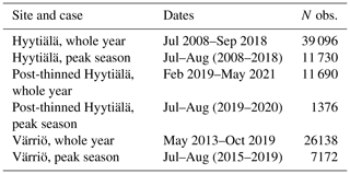
Data from Hyytiälä were divided into two separate data sets: pre-thinning, referred to just as Hyytiälä data (prior to 2019), and post-thinning (post 2019), referred to as post-thinning Hyytiälä data. The separation is due to the thinning of the forest at Hyytiälä station in 2019, which involved the removal of smaller trees from the forest understory, and additional thinning (from below) conducted from January to March 2020. In the thinning, 30 % of tree basal area was removed (Aalto et al., 2023), which significantly changed NEE due to the decrease in biomass. The data set thus had differences that were too large to be treated as a direct continuation of the pre-thinning data set. The amount of data points and the time intervals for each data set can be seen in Table 1.

Table 1 Summary of data sets: time periods and number of observations.

Table 2 List of input variables used for model training.

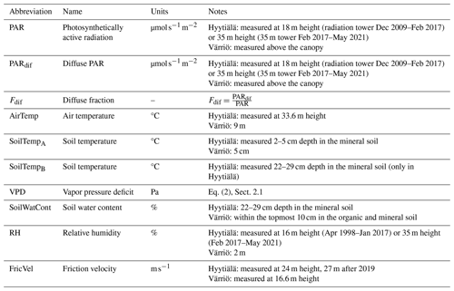
The data used in this study have a 30 min interval. The high frequency enables a more detailed study of the daily cycle of NEE. It allows for the analysis of the impact of such variables that affect the ecosystem processes on a short timescale, such as the impact of changes in radiation on photosynthesis. Raw measurements of the target variable (NEE) were collected using the eddy covariance technique (Aubinet et al., 2012) and then processed into NEE through the EddyUH software (Mammarella et al., 2016). Negative NEE corresponds to the ecosystem acting as a net carbon sink, while positive NEE corresponds to the ecosystem acting as a net carbon source. We model NEE using meteorological variables such as air temperature, soil temperature, solar radiation, relative humidity, and soil moisture content. The leaf area index (LAI) is not used here as its seasonal variability in the chosen period is relatively small (Hyytiälä about 30 %; Värriö 20 %), which translates to a below 10 % change in canopy light interception and roughly the same percentage in GPP. For some input variables, minor differences exist in how the data are measured at the two stations (e.g., soil moisture is from different depths). The data used were non-gap-filled to avoid the influence of models typically used for gap filling. At Hyytiälä, photosynthetically active radiation (PAR) was not measured before 2009, and we used global radiation multiplied by the PAR quantum efficiency of 2 $\mathrm{\mu }\mathrm{mol}{\mathrm{s}}^{-\mathrm{1}}{\mathrm{W}}^{-\mathrm{1}}$ (Ross and Sulev, 2000; Ezhova et al., 2018) to calculate missing values of PAR. All variables used are listed in Table 2.

In the pre-processing of the data, time points that contained missing values of any studied input variable were discarded. Also, all rows where the PAR value was less than 10 $\mathrm{\mu }\mathrm{mol}{\mathrm{s}}^{-\mathrm{1}}{\mathrm{m}}^{-\mathrm{2}}$ were filtered out due to the interest being solely on modeling daytime NEE. We calculated the diffuse fraction,

$$\begin{array}{}\text{(1)}& F_{\text{dif}}={\displaystyle \frac{{\text{PAR}}_{\text{dif}}}{\text{PAR}}},\end{array}$$

and vapor pressure deficit (Monteith and Unsworth, 2013),

$$\begin{array}{}\text{(2)}& \begin{array}{rl}\text{VPD}& =e_{\mathrm{s}}-e_{\mathrm{a}},\text{ where }\\ & e_{\mathrm{s}}=\mathrm{611}\exp \left({\displaystyle \frac{\mathrm{17.27}{T}_{\text{air}}}{\mathrm{237.7}+T_{\text{air}}}}\right),e_{\mathrm{a}}=e_{\mathrm{s}}{\displaystyle \frac{\text{RH}}{\mathrm{100}}}.\end{array}\end{array}$$

In Eq. (2), T_air is in degrees Celsius (°C) and e_s and e_a are in pascals (Pa).

Table 3 Overview of the training configurations for ML models across different data sets.

Table 4 List of the final model hyperparameters with their respective values for each modeling setup. Values of parameters are listed in the following order corresponding to different setups: Hyytiälä all, Hyytiälä peak, Värriö all, Värriö peak, mixed data sets with site label, and mixed data sets without site label.

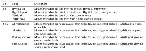
The machine learning models were trained in two sets of four setups (Table 3), and the results within a set were compared against each other. For both sets, four different machine learning models were trained for all of the four cases, meaning a total of 32 models trained. In the first set, models for data representing entire year and peak growth season (July and August) were trained using data from either pre-thinned Hyytiälä or Värriö. In the second set, models were trained by combining the data from two sites into a single mixed data set and then training them with and without variables that denote from which site the data originate from (“Värriö”, “Hyytiälä” for Hyytiälä pre-thinned, “HyytiäläT” for Hyytiälä post-thinned). Similarly to Set 1, setups included the entire year and peak growing season. A summary of the configurations for all experiments can be seen in Table 3.

In all cases, the data were split into training and test data, where training data were used to train the models, while test data were used to evaluate the models' performance. For modeling NEE for pre-thinned Hyytiälä and Värriö, 75 % of their respective data were used for training the model, while the rest were used as the test data to evaluate the model performance.In case of the mixed model, 80 % of the each respective data set was used to train the model. The processed data used for training the machine learning are publicly available at Laanti (2024).

2.2 Machine learning models

To ensure robustness and reduce potential biases, we validate our findings across four distinct ML models, aiming to identify consistent patterns or insights and provide an overall picture of how well the models can use these data to predict NEE. Applying several models to the same data set provides a context on what input variables are consistently considered important across different models. The four models used were cubist (Quinlan, 1992), random forest (Breiman, 2001), averaged neural network (Kuhn, 2008), and basic linear regression (Kutner et al., 2004). All were implemented in R (v. 4.3.0: https://www.r-project.org/, last access: November 2023) using R's “caret” library (v. 6.0.94: https://github.com/topepo/caret/, last access: November 2023). Linear regression served as the baseline model, while the other models were chosen due to their proven competence in solving various regression problems (Fernández-Delgado et al., 2019). The code used for training the machine learning models is publicly available at Laanti (2024).

Random forest (RF) is a popular model that has been used in previous research (Cai et al., 2020; Liu et al., 2021; Abbasian et al., 2022; Zhu et al., 2023) due to its ease of use, high accuracy, and robustness. It is an ensemble model that uses the averaged output of random regression trees (Fernández-Delgado et al., 2019) by training different regression trees on different subsets of the data. The final prediction is the average result of the different tree predictions. The algorithm is quite robust as the different trees are trained with the different subsets of the training data. The randomForest library (Liaw and Wiener, 2002) implements the regression algorithm of RF used in this study.

Cubist is one of the best-performing regression models (Fernández-Delgado et al., 2019) across multiple types of data sets (i.e., type and size of data). Like RF, it is created from multiple individual regression trees, where each terminal leaf contains a smoothed linear regression model for prediction (Zhou et al., 2019). It creates a series of if–then rules that can be considered the branches of a tree, while the leaves are an associated multivariate linear model. The corresponding model is used to calculate the final predicted value as long as the set of covariates satisfies the conditions of the corresponding rule. Cubist also uses boosting with its training committees, which creates a series of trees with different weights and nearest-neighbor search to adjust the predictions better.

Model-averaged neural networks (avNNet) are a single-hidden-layer feed-forward neural network characterized by its architecture and training approach. The network consists of interconnected neurons arranged in layers, with the final layer outputting the prediction (Ripley, 2007). During the training phase, initial weights, which influence predictions, are randomly assigned. These weights are then iteratively updated, enabling the network to capture nonlinear relationships. Given the randomness in predictions due to these initial weight assignments, avNNet constructs multiple neural network models and averages their results. This averaging process promotes a more robust and stable prediction by minimizing the impact of any single model's randomness.

The basic multivariate linear regression (LinRegr) is used as a baseline to understand how much impact and improved results more advanced models can provide. LinRegr finds a linear relationship between the independent and dependent variables determined by minimizing the sum of the squared differences between the predicted and the actual values (Hastie et al., 2009).

2.3 Cross-validation framework, hyperparameter tuning, and validation metrics

K-fold cross-validation is a resampling method for validating model efficiency, which generally results in less biased models (Jung, 2018). The K-fold cross-validation method shuffles the data set randomly and splits it into K groups or folds. First, each fold is taken as a holdout, while the model is fit on the rest of the folds, and then the model is evaluated on the holdout set. The score is retained, and the model is discarded. In repeated K-fold cross-validation, this process is done R times on different splits. K-fold cross-validation also effectively prevents model overfitting, where a machine learning model has learned to model the inherent noise of a data set, to a point where it fails to model for points not included in the training data set (Berrar, 2019).

During the model training, repeated K-fold cross-validation was used with caret libraries' (Kuhn, 2023) grid hyperparameter search. This method trains and evaluates a model using all possible combinations of specified hyperparameter values to identify the combination that yields the best model performance. It was used to tune the models' hyperparameters and configuration settings that are external to the model and can be adjusted to optimize performance. Values R=5 repeats and K=10 folds were used to fit each model. The tuned hyperparameters can be seen in Table 4. The train and test data as well as the folds of the K-fold cross-validation were split using a predetermined random split to ensure repeatability. However, due to technical limitations, in-depth hyperparameter tuning was not used on the models that contained data from all sites. Instead, hyperparameters based on the results from the single-site models were used.

In evaluating the performance of our machine learning models, we primarily relied on two key metrics to assess the models' goodness of fit: the coefficient of determination (R²) and the root mean squared error (RMSE). RMSE measures the differences between the values predicted by a model and the actual values and provides an understanding of the magnitude of error the model might make in its predictions. A lower RMSE indicates a better fit to the data, implying that the model's predictions are more precise. The models' hyperparameters were tuned specifically based on the RMSE score.

In addition, each model was trained on five different data splits to account for variability and reduce the influence of any single fortunate or unfortunate split on the results. The performance metrics, R² and RMSE, were averaged across these splits to ensure a robust and reliable assessment of model performance.

2.4 Explainable AI methods

As machine learning models have been used more in research and industry, the demand for more transparent and interpretable models has grown (Dwivedi et al., 2023). As model accuracy has risen, so has model complexity. The highly accurate and complex models have many hyperparameters that can not be made human-understandable. To be trustworthy, the ML model must produce interpretable or transparent results. Relying on unexplained or inaccurate predictions can lead to critical errors. Accuracy metrics do not always portray the true prediction capability of a model, so it is vital to critically evaluate the results against existing knowledge or theories. XAI methods aim to provide machine learning models and methods that enable users to better understand, analyze, and evaluate the models' decision-making.

In this study, we used two XAI methods: permutation feature importance and accumulated local effect (ALE) plots (Molnar, 2020). They provide insight into how the input variables affect a model's output. Both are model-agnostic global methods, meaning they can be used regardless of the selected model and provide interpretations on the data set as a whole rather than individual points (Molnar, 2020). Both of these methods were implemented using R's “iml” library (v.0.11.1: https://github.com/christophM/iml/, last access: November 2023, Molnar et al., 2018).

2.4.1 Permutation feature importance

Permutation feature importance is a method that aims to measure the increase in the prediction error of a model after the input variables (features) are permuted. In permutation feature importance, the relationship between a specific input variable and the variable the model tries to predict is deliberately disrupted to understand how the models' prediction accuracy is affected (Molnar, 2020). If an input variable is important, randomly rearranging its values increases the model error, as the model then relies on that specific input variable for an accurate prediction. The trained model is denoted as f, input variable matrix as X, target vector as y, and error measure as L(y,f(X)). The algorithm works as follows.

1. The original model error $e=L(\mathit{y},f(\mathbf{X}\left)\right)$ is estimated.

2. For each input variable with index $i\in \mathit{\{}\mathrm{1},\mathrm{\dots },p\mathit{\}}$, where p is the total number of input variables,

   • 2.1

     a permutated input variable matrix $\widehat{\mathbf{X}}$ is generated by permuting input variable i in the data X, which breaks the association between input variable i and the true outcome y;

   • 2.2

     the error caused by the permutation is estimated by predicting with it $\widehat{e}=L(\mathit{y},f(\widehat{\mathbf{X}}\left)\right)$; and

   • 2.3

     the permutation input variable importance is calculated as quotient ${\mathrm{Imp}}_i=\widehat{e}/e$.

3. Input variables are sorted by descending Imp.

Only test data are used to calculate the permutation feature importance. Assessing feature importance using the training data might result in scores that are too inflated due to a model overfitting on training data. That said, the features with very high scores might not be as important for making accurate predictions on new, unseen data. As with the metrics R² and RMSE, the permutation feature importance was calculated on multiple different data splits to ensure robustness of the results.

2.4.2 ALE plots

Accumulated local effect (ALE) plots describe how input variables influence the prediction of a machine learning model on average (Molnar, 2020). ALE reduces a complex machine learning function to a function that depends on only one, as in our case, or two input variables and visualizes the effects between a selected variable and the prediction of the target variable of a machine learning model. The idea is to remove the unwanted effects of other input variables, take partial derivatives (local effects) of the prediction function with respect to the feature of interest, and integrate (accumulate) them with respect to the same feature.

The value of ALE at a certain point can be thought of as the effect of the selected variable at a specific value compared to the average prediction made on the data. To calculate the ALE value for input variable s at point $x\in \left[\text{min}\right({\mathit{x}}_s),\text{max}({\mathit{x}}_s\left)\right]$, with x_s being the vector of this variable's values, the input variable values x_s are divided into K intervals, where the start of the first interval is the lowest value z₀=min(x_s), and the differences of predictions between the sequential intervals are calculated. While the exact ALE formula requires a model with a derivative, an approximate version is used here that is more widely adopted and works for models without a derivative. Initially, an uncentered effect is computed:

$$\begin{array}{rl}{\stackrel{\mathrm{‾}}{f}}_{s,\text{ALE}}\left(x\right)=& \sum _{k=\mathrm{1}}^{k_s\left(x\right)}{\displaystyle \frac{\mathrm{1}}{n_s\left(k\right)}}\sum _{i:x_s^{\left(i\right)}\in ]z_{k-\mathrm{1},s},z_{k,s}]}\left[f\right(z_{k,s},{\mathit{x}}_{-s}^{\left(i\right)})\\ & -f(z_{k-\mathrm{1},s},{\mathit{x}}_{-s}^{\left(i\right)})].\end{array}$$

The values x_s of input variable of interest s are replaced with grid values z_s, where the grid values represent the edges of the intervals. The interval index an input variable value x∈x_s falls in is denoted as k_s(x), while n_s(k) denotes the number of observations inside the kth interval of x_s. A single data point is denoted as ${\mathit{x}}^{\left(i\right)}=(x_s^{\left(i\right)},{\mathit{x}}_{-s}^{\left(i\right)}))$, where $x_s^{\left(i\right)}$ denotes the ith value for the selected input variable, and ${\mathit{x}}_{-s}^{\left(i\right)}$ is the vector of all the other features of a single data point that are kept constant. The ML predicting function is denoted as f.

The differences between the predictions $f(z_{k,s},{\mathit{x}}_{-s}^{\left(i\right)})-f(z_{k-\mathrm{1},s},{\mathit{x}}_{-s}^{\left(i\right)})$ are the effect that the input variable s has for an individual data point for predicting the dependent variable (NEE in our case) when using the upper and lower values of an certain interval. The sum ${\sum }_{i:x_s^{\left(i\right)}\in ]z_{k-\mathrm{1},s},z_{k,s}]}$ adds up the effects of all instances within an interval $x_s^{\left(i\right)}\in ]z_{k-\mathrm{1},s},z_{k,s}]$. This is then divided by the number of observations in this interval n_s(k) to obtain the average difference of the predictions of this interval. The sum ${\sum }_{k=\mathrm{1}}^{k_s\left(x\right)}$ accumulates the average effects across all intervals, meaning that the uncentered ALE of an input variable of interest is accumulated by all its previous intervals. After that, the effect is centered, making the mean effect zero:

$$f_{\mathrm{s},\text{ALE}}\left(x\right)={\stackrel{\mathrm{‾}}{f}}_{\mathrm{s},\text{ALE}}\left(x\right)-{\displaystyle \frac{\mathrm{1}}{n}}\sum _{i=\mathrm{1}}^n{\stackrel{\mathrm{‾}}{f}}_{\mathrm{s},\text{ALE}}\left(x_s^{\left(i\right)}\right).$$

The value of ALE can be thought of as the main effect of the input variable at a certain value compared to the average prediction of the data. The ALE plot has the advantage that it generates valid interpretations even if the variables are correlated – an issue that persists in other methods that reduce a prediction function f to a function that depends on a single input variable such as partial dependence plots or marginal plots (Molnar, 2020). As with permutation feature importance, only the test data set was used to reduce the chance of inflating scores due to a model overfitting on the training data set.

3 Results and discussion

3.1 NEE modeling for Hyytiälä and Värriö data sets

In this section, we report the results obtained with different models from Set 1 in Table 3 (pre-thinned Hyytiälä and Värriö, whole year and peak growing season). First, we assess models' performance with routinely used accuracy metrics (R² and RMSE), visualize diurnal and annual NEE cycles, and then use XAI methods. In each subsection, we start the discussion with the peak-growing-season results and continue with the whole-season results.

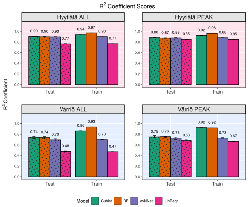
Figure 1 R² coefficients for all the models and different setups from Set 1 (Table 3). In each of the four panels, the results for the training data set are shown on the right (labeled “Train”), and the results for the test data set are shown on the left (dotted bars, labeled “Test”). Different colors are used to distinguish between the ML models; see legend. “ALL” denotes the scores for the models trained on the whole-year data sets; “PEAK” denotes the scores for the models trained on the peak-growing-season data sets. The black error bars show the min and max, and the bars show the mean of the scores trained on different splits of the data.

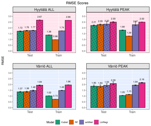
Figure 2 RMSE for all models and different setups from Set 1 (Table 3). In each of the four panels, the results for the training data set are shown on the right (labeled “Train”), and the results for the test data set are shown on the left (dotted bars, labeled “Test”). Different colors are used to distinguish between the ML models; see legend. “ALL” denotes the scores for the models trained on the whole-year data sets; “PEAK” denotes the scores for the models trained on the peak-growing-season data sets. The black error bars show the min and max, and the bars show the mean of the scores trained on different splits of the data.

3.1.1 Assessing model performance using accuracy metrics

Figures 1 and 2 show coefficients of determination and RMSE, respectively, for all the models, two stations, the peak growing season, and the whole year (Set 1 in Table 3). In general, the models perform better if trained on the Hyytiälä data set compared to the Värriö data set, as seen from higher R² coefficients. If the model is used on the training data set, the R² coefficients and RMSE are somewhat better than when used on the test data set, as expected. This effect is especially pronounced for RF and cubist models, which achieve high scores (R² > 0.85), largely because they are regression-tree-based models that tend to produce overly optimistic results on the data they were trained on. These high training scores do not reflect out-of-bag (OOB) performance, which typically provides a more accurate estimate of the model's true predictive ability on the data it was trained on (Kuhn and Johnson, 2013), due to OOB performance measuring not being available for all the models. The difference between the train and test scores is larger for Värriö than for Hyytiälä, as can be expected because the Värriö data set is smaller (Zhang et al., 2023). LinRegr and avNNet have almost identical scores on training and test data sets. The difference in scores between the training and test data sets is called a generalization error. In some cases, a large generalization error points to overfitting, i.e., the model learns the training data set too well and then performs poorly on the test data set. We applied K-fold cross-validation to avoid overfitting when choosing hyperparameters; see Sect. 2.3. Additionally, we tried different splits of the data into training and test data sets, which showed that the variation of the resulting R² coefficients and RMSE was small (Figs. 1 and 2). In addition, we obtained similar accuracy metrics on the test data sets using different nonlinear ML models, which also suggests that our results are robust. In what follows, the results are reported for the test data sets if not stated otherwise.

For the peak growing season, all four models perform well, including LinRegr, which is only slightly worse than the more complex models. For Hyytiälä, all nonlinear ML models give similarly high R² coefficients, close to 0.9, and RMSE values almost do not differ between these models. For Värriö, RF is slightly better than other ML models demonstrated by both a higher R² coefficient and a lower RMSE. Compared to Hyytiälä's R²=0.87, Värriö's R² coefficient is lower, R²≃ 0.70–0.74, which could be related to the higher share of outliers in the data or a smaller range of the predicted variable. The predictors vary within similar ranges in Hyytiälä and Värriö, whereas the predicted variable NEE has a larger value range in Hyytiälä compared to Värriö (corresponding to a weaker carbon sink in Värriö) because the Värriö ecosystem is less productive. It is also possible that the difference in R² coefficients could be because the available predictors have a more significant effect on the forest carbon balance in Hyytiälä than in Värriö. A decrease in R² coefficients for the cases when the predicted variable had a smaller value range was reported by other ML studies, e.g., Liu et al. (2021) and Abbasian et al. (2022). Also, for process-based models, reproducing carbon fluxes at less productive forests with low leaf area index is challenging (Mäkelä et al., 2019).

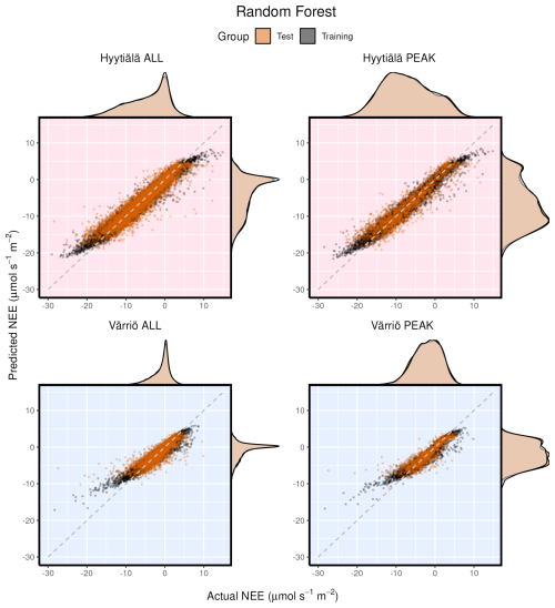
Figure 3 Modeled vs. measured NEE for Hyytiälä and Värriö on the example of the random forest model. Black points indicate training data sets; orange points indicate test data sets. “ALL” denotes the plots based on the whole-year data sets; “PEAK” denotes the plots based on the peak-growing-season data sets. The density distributions of the actual NEE and predicted NEE are shown on the top and right side of the plots, respectively, with colored being the test and translucent being the training data.

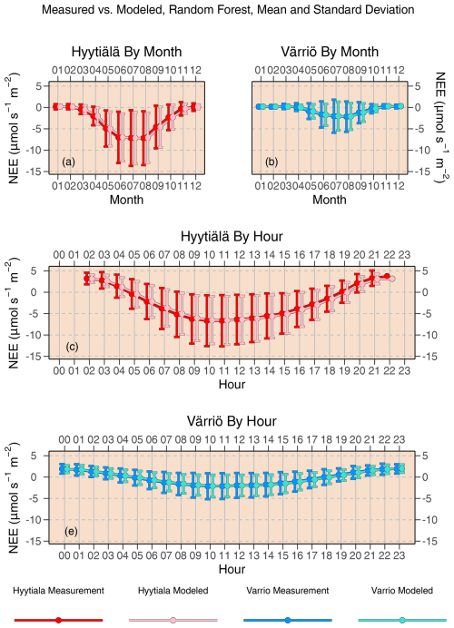
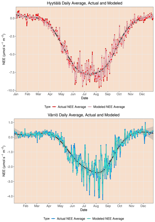
Figure 4 Mean diurnal and monthly cycles of daytime NEE as reproduced by random forest compared to actual NEE. Error bars denote standard deviation.

Scatter plots of measured vs. modeled data for training and test data sets are shown in Fig. 3 using one of the best-performing models, RF. The lowest modeled NEE values tend to be overestimated, and the highest modeled NEE values tend to be underestimated. This is seen best in the training data sets (because they are much larger) deviating from 1:1 lines at the extremes of the data. In Fig. 2, it is visible that RMSE values for Värriö are lower than those for Hyytiälä, which means that Värriö values in Fig. 3 are closer to the best-fit lines. Still, it does not mean that the model is better because the best-fit line of the measured vs. modeled data points is not 1:1. With high-accuracy scores, the mean diurnal cycle of NEE within the peak growing season is almost perfectly reproduced by the RF model (Fig. 4) with slightly smaller standard deviations in the modeled compared to the measured data.

Figure 5 Mean annual cycle of daily NEE as reproduced by random forest compared to actual NEE.

In the case of the whole-year data sets, the performance of LinRegr drastically decreases when compared to the peak-growing-season data sets (Figs. 1 and 2). This could be expected because, on the whole-year scale, NEE dependence on many variables becomes nonlinear. Especially for the Värriö data set, the LinRegr R² coefficient falls below 0.5, and RMSE increases by 40 % compared to the nonlinear ML models, meaning that more complex models are needed and justified. Figures 3–5 show scatter plots and annual daytime NEE cycle for Hyytiälä and Värriö. The same conclusions as for the peak-growing-season data sets apply here as the mean values were almost perfectly reproduced and extreme values were missing. The models captured the essential features of the annual NEE cycle, including ecosystem spring and autumn phenological transitions (Fig. 5).

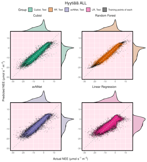
Figure 6 Modeled vs. measured NEE illustrating performance of all the models on the whole-year Hyytiälä data set. Black points indicate training data sets; orange points indicate test data sets. The density distributions of the actual NEE and predicted NEE are shown on the top and right side of the plots, respectively, with colored being the test, and translucent being the training data.

It is interesting to consider different models' performance for the same setup. Here we show an example for the Hyytiälä all setup (Fig. 6). The test cases for all nonlinear ML models look similar. Note orange points (test RF) covering black points (training RF) illustrating the smaller RMSE for the training data set in Fig. 6. The LinRegr plot is more scattered, and the points are not organized along one line (in agreement with reported low R² coefficients and high RMSE).

Compared to other studies, Dou and Yang (2018) demonstrated that in modeling whole-year NEE of forest ecosystems, the R² coefficients as high as 0.64–0.80 can be reached on the test data sets for separate evergreen needleleaf forest ecosystems. Our scores are within this interval for Värriö and significantly higher (0.90) for Hyytiälä. However, we used a different, more diverse set of input variables and modeled 30 min fluxes compared to daily fluxes in the study mentioned above. On a similar data set (deciduous forest in Germany, summer time, 30 min resolution), Moffat et al. (2010) got R²=0.93 and RMSE of 2.3 $\mathrm{\mu }\mathrm{mol}{\mathrm{s}}^{-\mathrm{1}}{\mathrm{m}}^{-\mathrm{2}}$ using an artificial neural network, which is close to Hyytiälä results.

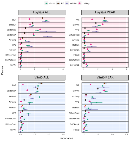
Figure 7 Feature importance for all the models and different setups from Set 1 (Table 3). The order of features is in accordance with the outcome of the random forest model. “ALL” denotes the plots based on the whole-year data sets; “PEAK” denotes the plots based on the peak-growing-season data sets. The points indicate the mean of the feature importance score across multiple data sets, while the bars show the min and max, respectively.

3.1.2 Which variables explain NEE: feature importance

We now consider feature importance, allowing us to analyze how the models rank input variables by their explanatory power. For the peak growing season, all nonlinear ML models agree for both stations (Fig. 7, Table A2) that the variables with the most explanatory power are PAR and diffuse PAR. Moreover, PAR typically comes first, except for cubist in the case of Värriö. Overall, during the peak growing season in boreal forests, a daytime CO₂ flux due to photosynthesis prevails over that due to respiration, at least in Hyytiälä (Kolari et al., 2009). Therefore, one can expect that parameters controlling photosynthesis also dominate the NEE response. PAR is theoretically the most important variable during the peak growing season to explain photosynthesis (Palmroth and Hari, 2001; Moffat et al., 2010), and the stimulating effect of diffuse radiation on the peak-season photosynthesis (diffuse radiation fertilization) is also well known (Gu et al., 2002). Accordingly, the models consider light-related variables to be the most important. Interestingly, LinRegr chooses diffuse PAR as the most important variable to explain NEE, likely because the dependence of photosynthesis on diffuse PAR can be considered closer to linear.

The third variable in importance after PAR and diffuse PAR, as seen by nonlinear models, is VPD (three cases), air temperature (two cases), or soil temperature A (one case). It is good to note that VPD is calculated based on air temperature (see Sect. 2.1), so these variables are not independent. PAR, diffuse PAR, and VPD are confirmed as essential drivers of carbon assimilation in numerous studies on photosynthesis in different ecosystems (Gu et al., 2002; Larcher, 2003; Grossiord et al., 2020). Particularly for Hyytiälä during the growing season, a statistical model showed that daily photosynthesis is most sensitive to light and VPD (Peltoniemi et al., 2015). However, as NEE is the net result of photosynthesis and respiration, and respiration is highly sensitive to temperature, it makes sense that the models pick either VPD or temperature as the third important variable. Ecosystem respiration is the sum of aboveground and belowground respiration, but soil temperature is sometimes considered a better parameter for modeling ecosystem respiration than air temperature (Kolari et al., 2009; Lasslop et al., 2012).

We note that nonlinear ML models typically place several variables close to the third position in the feature importance diagram. For Hyytiälä, RF places diffuse fraction close to VPD, followed by air temperature and RH; cubist and avNNet place intercorrelated soil temperature A and B (R=0.98, Fig. A1) high. For Värriö, cubist and avNNet place interdependent VPD, RH, and air temperature in the feature importance diagram within the error bar from each other. Relatively large error bars for these variables suggest that the models seem to have difficulties ranking them, as their order may likely change depending on the data split. At the same time, the error bars are smallest for RF, which seems more confident than other nonlinear models in its treatment of interdependent variables.

Suppose the model chooses one variable before another correlated one. In that case, the second one can be placed low in the feature importance diagram, as the model, in principle, does not need it anymore. This does not mean, however, that one of the correlated variables explains NEE clearly better than the other: for example, Moffat et al. (2010) showed, using an artificial neural network, that intercorrelated diffuse fraction and diffuse radiation (as well as intercorrelated VPD and RH) have the same explanatory power for the summertime forest NEE and can be used interchangeably. However, all our models place diffuse PAR higher than diffuse fraction, and they typically place VPD higher than RH.

Feature importance for the whole-year setups (Fig. 7) shows another set of most relevant variables lifting soil temperature at the expense of air temperature or VPD (nonlinear models; see Table A2). In many cases, soil temperature becomes the second important variable – sometimes even the first (avNNet, Hyytiälä). The increasing importance of the temperature-related variable is expected because, in the whole-year case, the model needs to capture the seasonality of carbon flux (Mäkelä et al., 2004, 2006), and soil temperature grows in summer and decreases in winter. However, the models' choice of soil temperature over air temperature requires additional explanation. Presumably, the soil temperature is positive during the warm season and nearly constant during winter in the presence of snow. This behavior is in line with NEE, which is also inhibited in winter. Air temperature, in contrast, may display significant variability also in winter. In addition, soil temperature limits plant water use and photosynthesis in spring and autumn (Wu et al., 2012; Lintunen et al., 2020). In the case of the LinRegr, PAR is no longer among the three most important variables, replaced by another soil temperature or diffuse fraction.

Figure 8 ALE plots for all the models (see legend); data sets correspond to the peak growing season in Hyytiälä (upper panels) and Värriö (lower panels).

3.1.3 How the models use input variables: ALE

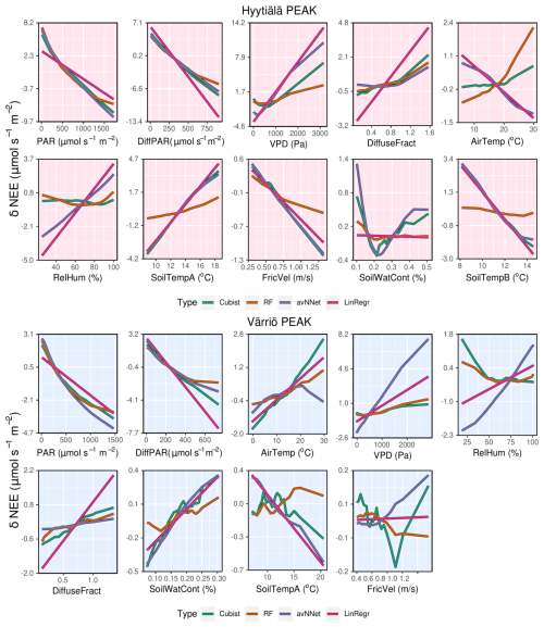
Proceeding with ALE, we discuss dependencies of NEE on input variables as seen by the models, focusing on the peak growing season so far. ALE demonstrates that NEE decreases with increasing PAR and diffuse PAR for all the models (Fig. 8). Nonlinear models show the nonlinear dependence of NEE on PAR, which is most pronounced for the RF model. This model shows that NEE saturates at higher PAR values, resembling the light response curve, and for the Värriö data set, NEE levels off at the largest diffuse PAR. This could be because high diffuse PAR is observed under a cloudy sky, and in Värriö, the corresponding PAR level can already be close to the light saturation point (Ezhova et al., 2018) inhibiting photosynthesis.

RF and cubist also capture a nonlinear dependence of NEE on VPD, which has an optimum value between the low and high values of VPD. At very high VPD, stomatal closure prevents plants from losing water (Running, 1976), also affecting photosynthesis. Besides, high VPD is often associated with high temperature, which increases NEE due to increased respiration. At low VPD, when water vapor pressure at the leaf level and in the atmosphere is about the same, there is no driving force to sustain transpiration. This inhibits water uptake by the roots and generally slows down plant metabolism, affecting photosynthesis. Moreover, low VPD is associated with lower PAR and higher diffuse fraction (Fig. A1), pointing at overcast cloudy conditions when photosynthesis is light-limited.

Note that dependencies of NEE on PAR, diffuse PAR, and VPD are qualitatively similar in all used nonlinear models, though quantitatively, sensitivity to the corresponding variables somewhat differs. However, the dependence of NEE on air temperature is not the same in all models. In Hyytiälä, RF and cubist feature an increase in NEE with air temperature, whereas LinRegr and avNNet demonstrate a decrease. In Värriö, all models except avNNet suggest a positive dependence of NEE on air temperature. The positive dependence is in line with the stomatal control at high temperatures (stomatal closure dampening photosynthesis) and higher soil respiration during the peak growing season.

It is interesting to analyze ALE from different models trained on the input data sets with several temperature variables. Both soil and air temperature are typically included in modeling studies of NEE based on machine learning (Dou and Yang, 2018; Liu et al., 2021; Abbasian et al., 2022). Cai et al. (2020) and Wood (2021) include average, minimum, and maximum air and soil temperature in their studies, adding more interdependent variables in the data sets. The Hyytiälä's data set includes air temperature and temperature from A and B soil horizons. In the peak season, all these temperature-related variables show quite similar dynamics. With soil depth, the mean temperature and amplitude of the diurnal temperature cycle decrease, and the time lag between the temperature signals increases. However, horizon B is not too deep, and the lag remains generally smaller than half a day. All the models, besides RF, treat soil temperatures A and B as important variables and demonstrate strong but opposite dependencies on these variables (Fig.8). As soil temperatures A and B are correlated (Appendix A, Fig. A1), opposite NEE dependencies must outweigh each other. Strong opposite dependencies on correlated variables should be treated cautiously as the models might use them to tune towards higher scores on given data sets. In the case of correlated soil temperatures, there is no guarantee that this compensation or tuning will work for even higher temperature, which is currently not represented in the data set. The same conclusion applies to using the model developed for a particular site on the data sets from other sites (Peltoniemi et al., 2015). In contrast, RF shows a strong association of NEE only with air temperature and a weak association with two soil temperature variables.

Now we briefly discuss other variables that have a more minor effect on NEE. Diffuse fraction demonstrates a consistent impact across all models, leading to some increase in NEE with its rise. This effect likely stems from the reduction of photosynthesis under an overcast sky with low radiation and high diffuse fraction. Note that diffuse fraction and diffuse PAR contain the same information provided PAR is included in the data set. Gross primary production in Hyytiälä has its minimum at the low diffuse PAR and a maximum at the high diffuse PAR compared to the weak parabolic dependence on diffuse fraction (Ezhova et al., 2018; Neimane-Šroma et al., 2024). That may be why the models choose diffuse PAR over diffuse fraction. Most models could then deem the diffuse fraction relatively unimportant as they already use diffuse PAR.

RH directly influences VPD through a linear relationship (Eq. 2, Fig. A1). The higher the RH, the closer ambient air is to saturation, and VPD, in this case, is small. Low RH, in contrast, favors higher VPD values. Having VPD as one of the powerful explaining variables should, in principle, diminish the role of RH, as is the case for RF and cubist. However, RH is placed relatively high in the feature importance for avNNet and LinRegr, which is also reflected in the significant range of NEE variability due to RH.

In Hyytiälä, all nonlinear models feature an increase in NEE with decreasing soil water content. In Värriö, all models feature an increase in NEE with increasing soil water content, and in Hyytiälä, cubist and avNNet demonstrate similar behavior. Note, however, that sensitivity to this variable is quite low for all models, indicating that soil moisture does not limit ecosystem functioning in current conditions. However, this could change in the future, which would perhaps not be captured by the models.

For friction velocity, all models indicate a consistent trend in Hyytiälä, where an increase in friction velocity leads to a decrease in NEE, suggesting that NEE flux is somewhat sensitive to changes in turbulence levels. On the one hand, this could indicate an eddy covariance problem (Moffat et al., 2010). On the other hand, this dependence might reflect physical processes: friction velocity has a weak increasing trend in Hyytiälä due to trees getting taller, which coincides with the weak, increasing trend in carbon uptake but not in respiration (Launiainen et al., 2022). In Värriö, there is no clear dependence between friction velocity and NEE. Generally, this variable holds limited importance in the overall model predictions, which is to be expected as filtering by friction velocity is applied to the data sets routinely during quality checks.

We proceed with the whole-year ALE plots: the dependencies of NEE on light variables (PAR, diffuse PAR) remain largely similar to those for the peak-growing-season setup (Fig. A3). Most nonlinear models (except avNNet on Hyytiälä data set) predict that the NEE dependence on air temperature has a minimum in the presence of negative temperatures in the data set, suggesting larger NEE during the cold season and the warmest summer periods. This might reflect the absence of photosynthesis in the cold season and the increased respiration accompanied by inhibited photosynthesis for the highest temperatures. In Hyytiälä, NEE dependence on soil temperature A also has a minimum. In Värriö, NEE decreases with increasing soil temperature until it plateaus at around 15 °C in the case of RF and avNNet. Note that for Hyytiälä, NEE dependencies on soil temperatures B and A are again of opposite sign for all models except RF. The LinRegr fails on the Hyytiälä data set, showing a weak association of NEE with air temperature but featuring lower NEE and stronger carbon sink at low, even negative, soil temperatures. The failure of LinRegr on the whole-year data could be due to its inability to capture the nonlinear dependence of NEE on temperature, which becomes significant on a whole-season scale.

Considering less critical variables, the dependencies remain mainly the same. In some cases, however, avNNet demonstrates dependencies inconsistent with expected behavior, e.g., featuring a stronger carbon sink under low-RH conditions. It is worth mentioning that the dependence on soil water content is quite complicated in Hyytiälä, with a minimum and a maximum. This could be related to data containing subsets with high water content at low temperatures when photosynthesis is inhibited, e.g., during snowmelt or late autumn. In any case, as for the peak-growing-season setup, the sensitivity of NEE to this variable is low.

Finally, if the most important input variables for the studied sites are the same and the dependencies of NEE on these variables are similar in the case of RF and, to a lesser extent, cubist, one could expect that it is possible to build a more generic model, which would be able to give reasonable results for many different boreal forest sites. We, therefore, built one model based on all the data in the following section.

3.2 NEE modeling: mixed data set

In this section, we report the results of NEE modeling using Set 2 (Table 3), which consists of mixed data from pre-thinning Hyytiälä (referred to just as Hyytiälä), Värriö, and post-thinning Hyytiälä. We aimed to understand how the models perform in the following cases: (1) mixed data set, containing data from both sites without any separation or benchmarking the data (peak without site and all without site setups, Table 3); (2) mixed data set, but we introduce three binary dummy variables that identify the site (peak with site and all with site setups, Table 3). Three binary variables were used instead of a single categorical one due to some models requiring real numbers as input (Hancock and Khoshgoftaar, 2020).

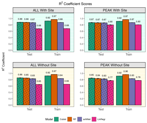
Figure 9 R² coefficients for all the models and different setups from Set 2 (Table 3). In each of the four panels, the results for the training data set are shown on the right (labeled “Train”), and the results for the test data set are shown on the left (dotted bars, labeled “Test”). “ALL” denotes the scores for the models using the whole-year data sets; “PEAK” denotes the scores for the models using the peak-growing-season data sets. “With Site” indicates the input variables contain information about the site; “Without Site” indicates the input variables contain no information about the site. The black error bars show the min and max, and the bars show the mean of the scores trained on different splits of the data.

3.2.1 Assessing model performance on a mixed data set using accuracy metrics

The determination coefficients for mixed data sets are shown in Fig.9, separately for the model runs with and without the variables for the site identity. Adding site variables to the data set slightly improves the correlation coefficient R² (within 3.5 %), which remains high for the best models, RF and cubist (0.84–0.87 for the peak season, 0.86–0.89 for the whole season). Comparing this result to the results for the separate stations (Fig. 1), we note that the scores are closer to those for Hyytiälä. This could be because Hyytiälä data prevail in the compiled data set. However, a trial run with equal inputs from different sets (Hyytiälä pre-thinned + Hyytiälä post-thinned + Värriö) shows that R² was only marginally lower, by 0.02 for the nonlinear ML models (Figs. A5 and A6). This finding suggests that factors other than the prevalence of the Hyytiälä data set may be important: for example, the value range of the data. The Hyytiälä data set has a larger NEE value range compared to Värriö, and that could be the reason for the better Hyytiälä R² coefficient, as mentioned in Sect. 3.1.1. Therefore, one could expect larger R² coefficients for any mixed sets containing a sufficient amount of Hyytiälä data when compared to the Värriö data set. Interestingly, LinRegr performs worse than other models on a compiled data set, even for the peak growing season. The LinRegr R² coefficient on the mixed data set is clearly lower than on the Hyytiälä data set (drop from 0.85 to 0.80 for the peak growing season and from 0.76 to 0.68 for the whole year).

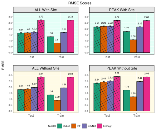
Figure 10 RMSE for all the models and different setups from Set 2 (Table 3). In each of the four panels, the results for the training data set are shown on the right (labeled “Train”), and the results for the test data set are shown on the left (dotted bars, labeled “Test”). “ALL” denotes the scores for the models using the whole-year data sets; “PEAK” denotes the scores for the models using the peak-growing-season data sets. “With Site” indicates the input variables contain information about the site; “Without Site” indicates the input variables contain no information about the site. The black error bars show the min and max, and the bars show the mean of the scores trained on different splits of the data.

As previously stated, site variables do not have a significant effect on R² coefficients, but the advantage is more evident for RMSE (Fig. 10). RMSE for the peak-growing-season data is generally larger than for the whole season, likely because the fluctuations and errors of NEE measurements outside the growing season are relatively small. In addition, the flux random error increases with the flux magnitude within the growing season. If we compare the models with and without site variables, we see that adding site variables reduces RMSE by 10 %–13 %: from about 2.4 to 2.15 $\mathrm{\mu }\mathrm{mol}{\mathrm{s}}^{-\mathrm{1}}{\mathrm{m}}^{-\mathrm{2}}$ for the peak growing season and from about 1.8 to 1.6 $\mathrm{\mu }\mathrm{mol}{\mathrm{s}}^{-\mathrm{1}}{\mathrm{m}}^{-\mathrm{2}}$ for the whole year. Considering models trained on data of separate sites, RMSE scores in the models with site variables are somewhat smaller compared to the models trained on the Hyytiälä data set, probably due to the presence of Värriö data with smaller RMSE than Hyytiälä data (Fig. 2) or due to the larger size of the mixed data set. Overall, introducing the site variables in the mixed data set barely improves the correlation between measured and modeled points but reduces the scatter in the plot presenting measured vs. modeled points.

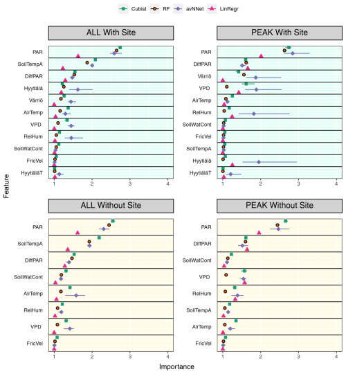
Figure 11 Feature importance for all the models trained on the mixed data sets containing (“With Site”) and not containing (“Without Site”) site variables. The order of features is in accordance with the outcome of the random forest model. “ALL” denotes the plots based on the whole-year data sets; “PEAK” denotes the plots based on the peak-growing-season data sets. The points indicate the mean of the feature importance score across multiple data sets, while the bars show the min and max, respectively.

3.2.2 Feature importance for the mixed data set

We assess the feature importance diagrams provided by the models on the mixed data sets, paying special attention to the ranking of the site variables (Fig. 11, Table A2). It follows quite clearly from Table A2 that the models' choice of the most important input parameters becomes more aligned when they are trained on the mixed data set. For example, all the models, without exception, choose PAR as the most important variable in both the peak-season and the whole-year setups. During the peak season, the second variable in the feature importance diagrams is diffuse PAR (six setups out of eight) or VPD (two out of eight). Continuing with the peak season, site parameter “Värriö” appears only as the third variable in the corresponding setups (replaced in some models with VPD or diffuse PAR). In the setup without site parameters, the third important variable is VPD or diffuse PAR or soil water content in case of RF. The latter observation is interesting as Värriö has different soil characteristics: soil moisture is lower there (Fig. A2), and RF might have used it as a replacement of the site variable.

For the whole-year setups, the second variable after PAR in the feature importance diagrams is almost always soil temperature A (seven out of eight cases) or diffuse PAR (one out of eight cases). (Recall that the Hyytiälä feature importance set contained soil temperature B and not A. Replacement of this variable by the temperature at A horizon is because soil temperature B is not in the data set anymore as it was not measured in Värriö.) The third variable is diffuse PAR (five out of eight cases) or VPD/soil temperature/air temperature (one case each). Note that site variables are not among the three most important in the whole-season setups. Instead, the models retain NEE dependence on soil temperature, which allows them to reproduce a seasonal cycle and choose over the site variables diffuse PAR, VPD, or air temperature. Nevertheless, site variables appear among the six highest input variables in the feature importance diagrams, and as follows from Fig.10, they help to reduce the RMSE.

Another observation is that among site variables, the models put “Värriö” highest in the peak-season setups but “Hyytiälä” in the whole-year setups. However, as mentioned before, it should be possible for the models to use them interchangeably.

Figure 12 ALE plots for all the models trained on the mixed data sets containing (“With Site”, lower panels) and not containing (“Without Site”, upper panels) site variables. The data sets are from the peak growing season.

3.2.3 ALE for the mixed data set

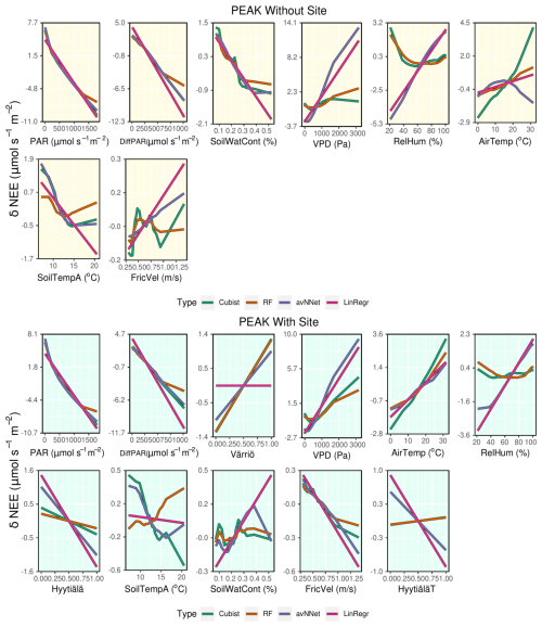
Judging by ALE (Figs. 12, A4), dependencies of NEE on light variables (PAR and diffuse PAR) for all setups in Set 2 are similar to those for separate stations (Figs. 8 and A3). In the peak season, the nonlinear models suggest that the third important variable is “Värriö” for the setups with site parameters. From Fig. 12, it can be seen that the modeled NEE increases if “Värriö” changes from zero to one. The models then use this site variable to make all NEE values at Värriö somewhat higher than the general mean value for all three sites, which is the case due to lower tree biomass. Similarly, models use the variable “Hyytiälä” when it is equal to one to decrease NEE, and this decrease is less pronounced for cubist and RF than for the other models. Finally, when the “HyytiäläT” variable is equal to one, RF and cubist slightly increase NEE, whereas the other models decrease NEE. Because the prevailing data set is still Hyytiälä pre-thinned, this data set likely dictates the base values chosen by the models. Therefore, a moderate increase in NEE for the Hyytiälä thinned data set and a stronger NEE increase for the Värriö station is reasonable. Interestingly, LinRegr does not use the site variable “Värriö” at all.

In the peak-season setup without site variables, soil water content is one of the relevant variables chosen by the models, especially RF. Judging by ALE (Fig. 12), the models prescribe higher values of NEE to the drier cases, which is in line with how the ecosystem functions under drier conditions (reduction of photosynthesis). Similarly, for the whole-season setup without site variables, we note that NEE decreases strongly with increasing soil water content (Fig. A4), in contrast to what was observed when we modeled separate sites. ALE plots for both the peak-season and whole-season setups (Figs. 12 an A4) demonstrate clearly how soil water content loses its strong position when site variables are introduced and how the NEE dependence on this variable again becomes complex, in line with what is observed for separate stations.

NEE dependencies on VPD are qualitatively similar for mixed data sets in those for separate sites. LinRegr and avNNet still have strong and opposite NEE dependencies on VPD and RH, similar to their performance on the Hyytiälä data set. These models might use variable RH to compensate for a modeled effect of VPD on NEE that is too strong.

Interestingly, all models display a positive dependence of NEE on air temperature for the peak growing season and setup with site variables, unlike avNNet and LinRegr on Hyytiälä data. Positive dependence is in line with theoretical expectations due to increasing respiration and reduced photosynthesis with increasing temperature within the peak season. At the same time, NEE somewhat decreases with increasing soil temperature A for all the models except RF; however, this effect of soil temperature on NEE, as captured by the models, is much weaker than that of air temperature.

On the whole-year scale, all nonlinear models demonstrate rather similar NEE dependencies on different variables (except strong NEE dependencies on VPD and RH partially outweighing each other as modeled by avNNet), which was also the case for the separate Värriö setup. This could be due to the data from Värriö that have a long dormant season: one of the main tasks of the models is to reproduce seasonal cycle, for which the nonlinear models use soil temperature in a similar manner.

Generally, RF performed more in line with theoretical expectations from ecophysiological research than other models when trained on the data set containing interdependent variables. LinRegr and the avNNet demonstrate strong dependencies of NEE on VPD, which they likely compensate for with relatively strong dependencies of NEE on air temperature and RH. Due to that, some ALE may appear counterintuitive (e.g., strengthening of carbon sink with increasing air temperature during the peak season), contradicting the expectations based on general knowledge of ecosystem functioning. In addition, all models except RF demonstrate strong opposite associations with soil temperature A and B when both variables are available (Fig. 8).

4 Conclusions

We modeled NEE at two sites in boreal forests: one in central Finland and one in the Finnish subarctic. We focused on the peak-growing-season and whole-year data sets. Peak-growing-season NEE for separate sites can be modeled reasonably well even with a simple linear regression model. However, linear regression performs significantly worse than nonlinear ML models in the case of the mixed data sets from both sites or whole-year data sets.

The most powerful explaining variables in the peak-growing-season setups are PAR, diffuse PAR, and vapor pressure deficit (or air temperature); in the case of the whole-year setups, such variables are PAR, soil temperature, and diffuse PAR. This is a robust result reproduced by most of the models used in this study. High vapor pressure deficit dampens photosynthesis and, hence, makes NEE increase. This effect is essential during the peak growing season. The models presumably used soil temperature to account for the change in NEE within a seasonal cycle.

To build a joint model for several sites, we added site variables. The model is more sensitive to these variables within the peak growing season, whereas soil temperature retains its importance for the whole-year data sets. In the absence of site-specific variables, random forest ranks soil water content, the variable that differs most between the sites, as the third most important in the feature importance diagram. NEE dependence on soil water content and the importance of this variable for NEE predictions change drastically for the models built on the data sets, including and excluding site variables.

Our ALE results suggest that cubist and especially random forest display more robust behavior modeling complex nonlinear dependence of net ecosystem exchange on the set of interconnected variables. They could qualitatively reproduce the theoretically expected dependencies of NEE on the major climatic drivers of ecosystem processes under different conditions and for several sites. This result aligns with many studies that used random forest based on its best performance compared with other models. Additionally, linear regression and model-averaged neural networks tend to overemphasize certain variables while compensating with other interdependent variables. In our modeling study, linear regression and model-averaged neural networks compensated using variables like air temperature and relative humidity, which are highly sensitive to changing climate conditions.

All in all, it should be noted that the models' performance changes depending on a given setup, so no single recommendation suggesting or prohibiting a specific model can be given. This is, instead, a case-by-case issue. Therefore, we call for broader usage of explainable artificial intelligence methods when applying ML methods, especially when choosing the most suitable model. Feature importance and ALE plots together allow for a direct comparison between ML model functioning and process-based models.

Finally, we showed that even a simple way to account for the difference between the sites decreases RMSE and improves the model. The next step is to introduce a more suitable variable, allowing us to distinguish the ecosystems from each other. As Hyytiälä data are split into pre-thinned and post-thinned, we need a variable that could account for this change in the vegetation. The best candidates for this could be the satellite-based normalized difference vegetation index (NDVI) and LAI (Launiainen et al., 2022; Zhu et al., 2023), which we plan to add to our data set instead of site variables.

Appendix A

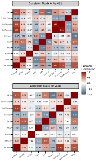
Figure A1 Heat maps illustrating linear correlation between input variables in Hyytiälä and Värriö. Statistically insignificant correlations are marked with an asterisk (*).

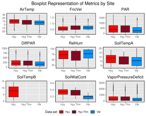
Figure A2 Box plots of input variables comparing Hyytiälä and Värriö data sets on the whole-year timescale. “Hyy” refers to the Hyytiälä pre-thinned data set, “Hyy Thin” refers to the Hyytiälä post-thinned data set, and “Vär” refers to the Värriö data set.

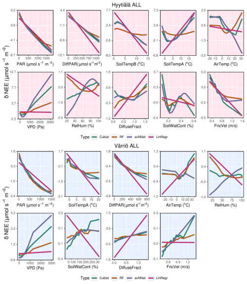
Figure A3 ALE plots for all the models trained on the whole-year data sets from Hyytiälä (upper panels) and Värriö (lower panels).

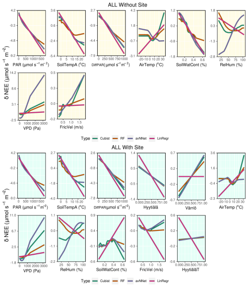
Figure A4 ALE plots for all the models trained on the mixed data sets containing (“With Site”) and not containing (“Without Site”) site variables. The data sets are from the whole year.

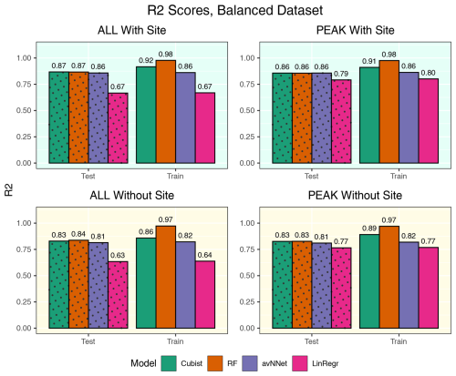
Figure A5 R² coefficients for all the models and different setups from Set 1 (Table 3). Here, the models were trained using equal amount of data points from Hyytiälä, Värriö, and post-thinning Hyytiälä (balanced data sets). In each of the four panels, the results for the training data set are shown on the right (labeled “Train”), and the results for the test data set are shown on the left (dotted bars, labeled “Test”). “ALL” denotes the scores for the models using the whole-year data sets; “PEAK” denotes the scores for the models using the peak-growing-season data sets. “With Site” indicates the input variables contain information about the site; “Without Site” indicates the input variables contain no information about the site.

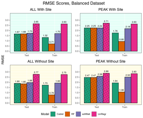
Figure A6 RMSE for all the models and different setups from Set 1 (Table 3). Here, the models were trained using equal amount of data points from Hyytiälä, Värriö, and post-thinning Hyytiälä (balanced data sets). In each of the four panels, the results for the training data set are shown on the right (labeled “Train”), and the results for the test data set are shown on the left (dotted bars, labeled “Test”). “ALL” denotes the scores for the models using the whole-year data sets; “PEAK” denotes the scores for the models using the peak-growing-season data sets. “With Site” indicates the input variables contain information about the site; “Without Site” indicates the input variables contain no information about the site.

Table A1 Three most important features for different models and Set 1 (Table 3).

Table A2 Three most important features for different models and Set 2 (Table 3).