Hot spots, hot moments, and spatiotemporal drivers of soil CO₂ flux in temperate peatlands using UAV remote sensing

CO₂ emissions from peatlands exhibit substantial spatiotemporal variability, presenting challenges for identifying the underlying drivers and for accurately quantifying and modeling CO₂ fluxes. Here, we integrated field measurements with Unmanned Aerial Vehicle (UAV)-based multi-sensor remote sensing to investigate soil respiration across a temperate peatland landscape. Our research addressed two key questions: (1) How do environmental factors control the spatiotemporal distribution of soil respiration across complex landscapes? (2) How do spatial and temporal peaks (i.e., hot spots and hot moments) of biogeochemical processes influence landscape-level CO₂ fluxes? We find that dynamic variables (i.e., soil temperature and moisture) play significant roles in shaping CO₂ flux variations, contributing 43 % to seasonal variability and 29 % to spatial variance, followed by semi-dynamic variables (i.e., Normalized Difference Vegetation Index (NDVI) and root biomass) (19 % and 24 %). Relatively static variables (i.e., soil organic carbon stock and carbon to nitrogen ratio) have a minimal influence on seasonal variation (2 %) but contribute more to spatial variance (10 %). Additionally, predicting time series of CO₂ fluxes is feasible by using key environmental variables (test set: coefficient of determination (R²) = 0.74, Root Mean Square Error (RMSE) = 0.57 $\mathrm{\mu }\mathrm{mol}{\mathrm{m}}^{-\mathrm{2}}{\mathrm{s}}^{-\mathrm{1}}$, Kling-Gupta Efficiency (KGE) = 0.77), while UAV remote sensing is an effective tool for mapping daily daytime soil respiration (test set: R²=0.75, RMSE = 0.56 $\mathrm{\mu }\mathrm{mol}{\mathrm{m}}^{-\mathrm{2}}{\mathrm{s}}^{-\mathrm{1}}$, KGE = 0.83). By the integration of in-situ high-resolution time-lapse monitoring and spatial mapping, we find that despite occurring in 10 % of the year, hot moments (i.e., periods of time which have a disproportional high (>90th percentile) CO₂ fluxes compared to the surrounding) contribute 28 %–31 % of the annual CO₂ fluxes. Meanwhile, hot spots (i.e., locations which CO₂ fluxes higher than 90th percentile) – representing 10 % of the area – account for about 20 % of CO₂ fluxes across the landscape. Our study demonstrates that integrating UAV-based remote sensing with field surveys improves the understanding of soil respiration mechanisms across timescales in complex landscapes. This will provide insights into carbon dynamics and supporting peatland conservation and climate change mitigation efforts.

1 Introduction

Peatlands are globally distributed ecosystems that cover an area of 6.75 million km² and store 942.09±312 Gt of carbon (Widyastuti et al., 2025). However, rising concerns exist over peatlands shifting from carbon sinks to carbon sources due to the impact of climate change (Dorrepaal et al., 2009; Huang et al., 2021; Hopple et al., 2020), land use/cover conversion (Leifeld et al., 2019; Deshmukh et al., 2021; Prananto et al., 2020), and other disturbances (Wilkinson et al., 2023; Turetsky et al., 2015). In Europe, it has been reported that nearly half of the peatlands are suffering degradation, primarily due to drainage for agricultural or forestry activities (Leifeld et al., 2019; UNEP, 2022). As a consequence, European peatlands currently emit up to 580 Mt CO_2 eq. per year across the continent (UNEP, 2022). Given the critical role of the peatland ecosystem in the terrestrial carbon cycle, it is therefore important to understand the mechanisms driving carbon fluxes and their responses to climate change and human disturbances.

Soil respiration, a key ecological process that releases CO₂ from peatlands into the atmosphere, is influenced by a combination of biotic and abiotic factors. Among abiotic controls, soil temperature and moisture play a crucial role in driving microbial activity and root respiration, influencing CO₂ fluxes across daily to annual scales(Evans et al., 2021; Fang and Moncrieff, 2001; Hoyt et al., 2019; Juszczak et al., 2013; Swails et al., 2022). Water table fluctuations alter oxygen availability and distribution within the soil profile, directly affecting microbial processes and carbon emissions (Evans et al., 2021; Hoyt et al., 2019). Atmospheric pressure affects the transport of gases between the soil surface and the atmosphere, thereby modulating the CO₂ fluxes (Lai et al., 2012; Ryan and Law, 2005). Vegetation, as a key biotic factor, influences the spatiotemporal variations of soil respiration through phenology, structure, and community (Acosta et al., 2017; Wang et al., 2021). In addition, soil organic matter provides essential substrates for microbial activity, with previous studies suggesting that the quality of organic material, rather than its quantity, primarily regulates CO₂ fluxes in peatlands (Hoyos-Santillan et al., 2016; Leifeld et al., 2012).

CO₂ emissions from peatlands are highly variable over space and time, presenting challenges to accurately quantify and model carbon fluxes. This may be partially because peatlands are characterized by a unique microtopography, including features such as hummocks and hollows (Moore et al., 2019). These small-scale variations create differences in hydrology, temperature, biogeochemistry, and vegetation (Harris and Baird, 2019), leading to substantial spatial differences in the factors that control CO₂ fluxes and the formation of “hot spots” with elevated CO₂ emissions (Kelly et al., 2021; Becker et al., 2008; McClain et al., 2003; Frei et al., 2012; Kim and Verma, 1992). In addition, peatlands exhibit a high sensitivity to meteorological variability, which can trigger periods of disproportionately high CO₂ fluxes – often referred to as “hot moments” – in response to transient environmental changes, such as sudden shifts in temperature, atmospheric pressure, rainfall events, or fluctuations in the water table (Anthony and Silver, 2023; Fernandez-Bou et al., 2020). High CO₂ emissions occur from discrete areas in space (hot spots) and over short periods (hot moments), and may disproportionately contribute to the overall fluxes (Anthony and Silver, 2023; Fernandez-Bou et al., 2020). Most studies have examined the mechanisms and contributions of hot spots and hot moments of other greenhouse gases (N₂O, CH₄) in agricultural and forestry ecosystems (Krichels and Yang, 2019; Anthony and Silver, 2021; Kannenberg et al., 2020; Leon et al., 2014; Fernandez-Bou et al., 2020). However, research on CO₂ emission hot spots and hot moments in peatlands remains limited (Anthony and Silver, 2023), even though both CO₂ and CH₄ originate from organic matter decomposition under different redox conditions.

Identifying and quantifying hot spots and hot moments in peatlands is challenging, requiring large-scale, continuous, long-term observations. Currently, most studies on peatland soil respiration rely on point measurements taken at intervals of half a month to one month, primarily during daytime (e.g., Wright et al., 2013; Bubier et al., 2003; Kim and Verma, 1992; Danevčič et al., 2010). This spatiotemporal limitation constrains the effective understanding of hot spots and hot moments. Some studies attempted to extrapolate point data using land-use maps (van Giersbergen et al., 2024; Webster et al., 2008; McNamara et al., 2008), but uncertainties in landscape-scale fluxes increase as the number of measurement locations decreases (Arias-Navarro et al., 2017; Wangari et al., 2022; Gachibu Wangari et al., 2023). While automated chamber systems improve temporal resolution and help capture hot moments (Hoyt et al., 2019; Anthony and Silver, 2023), they are typically limited to a few sampling points, and scaling up is constrained by significant resource demands. Eddy covariance towers can continuously measure net ecosystem exchange over large areas (Rey-Sanchez et al., 2022; Abdalla et al., 2014), but they are less effective in capturing the spatial heterogeneity of peatlands (Lees et al., 2018). These limitations highlight the need for spatially robust, high-resolution methods that can characterize CO₂ fluxes across heterogeneous landscapes.

Several studies have integrated satellite-based remote sensing datasets with on-site chamber measurements to model landscape-scale CO₂ fluxes (e.g., Junttila et al., 2021; Gachibu Wangari et al., 2023; Lees et al., 2018; Azevedo et al., 2021). Remote sensing datasets on topography and vegetation parameters serve as proxies for soil moisture, vegetation cover, and nutrient availability, enabling large-scale CO₂ emission estimates within peatlands (Lees et al., 2018). However, this approach is somewhat limited by coarse spatial (10 m to 1 km) and temporal (1 to 16 d) resolutions, which may overlook hot spots and hot moments, leading to potential over- or underestimations of CO₂ fluxes in heterogeneous (e.g., complexity in topography, diverse vegetation types, varying thermal-hydrological conditions) peatlands (Kelly et al., 2021; Simpson, 2023). This shortcoming might be overcome by using unmanned aerial vehicles (UAVs) equipped with different kinds of sensors such as Red-Green-Blue (RGB), multispectral, thermal infrared, and Light Detection and Ranging (LiDAR). UAVs offer flexible deployment and capture high-resolution spatiotemporal data (1 cm to 1 m, minutes to months) (Minasny et al., 2019) which makes them particularly suitable for monitoring complex peatland dynamics and detecting hot spots and hot moments. Thus far, UAVs have proven to be reliable tools for peatland applications, including vegetation mapping (Steenvoorden et al., 2023), topographic reconstruction (Harris and Baird, 2019), peat depth and carbon storage estimation (Li et al., 2024), ground-water and surface water interactions (Moore et al., 2024), and moisture monitoring (Henrion et al., 2025). In a recent study, Kelly et al. (2021) utilized UAV-derived land surface temperature to estimate ecosystem respiration of a hemi-boreal fen in southern Sweden, and some studies (e.g., Pajula and Purre, 2021; Walcker et al., 2025) employed UAV-based multispectral vegetation indices to map ecosystem CO₂ flux at high resolution. These recent studies demonstrated the great potential of UAVs for linking CO₂ fluxes with environmental factors at a very high resolution, although they mainly focused on data from a single sensor. Few studies have explored the fusion of UAV-derived data from multiple sensors for mapping soil respiration across peatland landscapes.

In this study, we integrate multi-sensor UAV-based remote sensing with traditional field surveys to investigate soil respiration across a temperate peatland bog landscape, located in the Belgian Hautes Fagnes, which represents an important ecosystem for studying peatland carbon fluxes due to its sensitivity to climate change and hydrological dynamics. Our research addresses two key questions:

1. What controls the nature and strength of the relationship between soil respiration and environmental factors – such as thermal-hydrological conditions, vegetation, carbon stock and quality – across complex peatland landscapes and across spatiotemporal scales? To address this, we first identify the factors driving seasonal and spatial variations in soil respiration and then assess the potential for linking environmental factors to CO₂ flux at high spatiotemporal resolutions.

2. How do spatial and temporal peaks (i.e., hot spots and hot moments) of biogeochemical processes influence landscape-level carbon fluxes? For this purpose, we analyze the locations and timing of hot spots and hot moments, and assess their contributions to overall CO₂ flux budgets.

2 Materials and methods

2.1 Study site

The Belgian Hautes Fagnes plateau, part of the Stavelot-Venn Massif, is located in eastern Belgium (Fig. 1a). This elevated landscape experiences a humid climate, with mean annual air temperature and precipitation being approximately 6.7 °C and 1439.4 mm (period: 1971–2000), respectively (Mormal and Tricot, 2004). The peatlands in this region cover an area of 37.50 km², which primarily consist of raised bogs formed since the Late Pleistocene and grown under both oceanic and continental influences (Frankard et al., 1998; Goemaere et al., 2016). Our study site (50.49° N, 6.05° E; ∼0.30 km²) is located in the upper valley of the Hoëgne River peatland bog region (Fig. 1a). This ombrotrophic bog is mainly fed by precipitation and covers an area of approximately 32 ha. The landscape exhibits complex structures, characterized by distinct SE-NW oriented topographic units (i.e., summit, topslope, shoulder, backslope, and footslope), along with diverse microtopographic features, spatiotemporal varying thermal-hydrological conditions, differences in peat thickness and carbon storage, and a range of vegetation types (Sougnez and Vanacker, 2011; Henrion et al., 2024; Li et al., 2024). More specifically, the summit is a low-relief, southeast-facing plateau at 675–680 m elevation, which transitions downslope into the topslope and concave shoulder slope positions (Fig. 1a). The northwest-facing backslope is relatively steeper (average slope grade: 4.98°; elevation range: 645–670 m) compared to these upper units, while the footslope lies in the northwestern hillslope adjacent to Hoëgne River. The peat thickness varies spatially from 0.20 to 2.10 m across the landscape, with deeper deposits in the footslope and shallower peat at the topslope (Henrion et al., 2024; Li et al., 2024). The estimated soil organic carbon (SOC) stocks (i.e., top 1 m layer) range from 176.13 to 856.57 t ha⁻¹, with significantly higher storage at the summit, shoulder, and footslope (Li et al., 2024). Due to the pronounced topographic gradients and microtopography, the landscape exhibits great spatiotemporal variability in rootzone soil volumetric water content (range: 0.1–1 cm³ cm⁻³) and water table dynamics (range: −80–5 cm) (Henrion et al., 2025). The study site was drained and planted with spruces in 1914 and 1918, while the plantations were progressively cleared between 2000 and 2016. Since 2017, the site has been under restoration and now primarily covered by Vaccinium myrtillus, Molinia caerulea, Juncus acutus, and native hardwood species (e.g., Betula pubescens and Quercus robur), as shown in Fig. 1b. An observation station of the Royal Meteorological Institute of Belgium (Mont Rigi, 50.51° N, 6.07° E) situated 3.07 km northeast of the study site, records rainfall and atmospheric pressure data every 10 min.

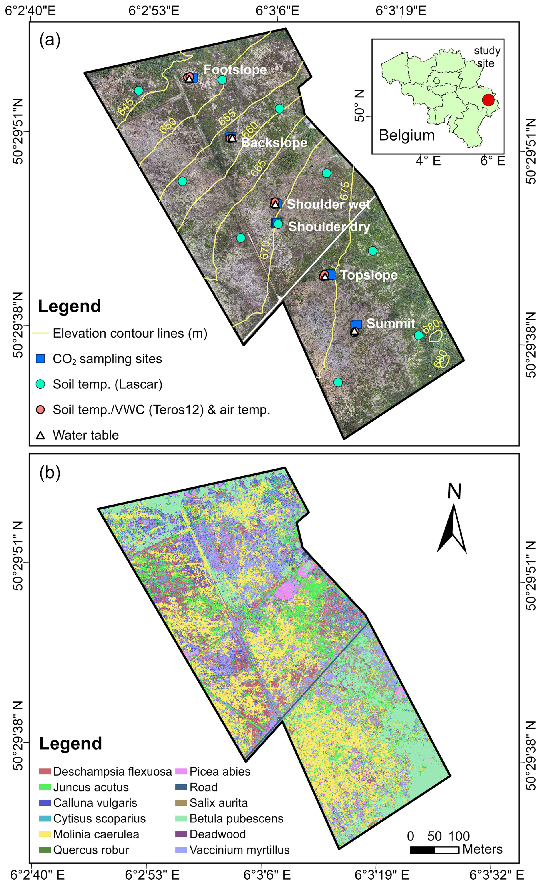
Figure 1 Maps showing the field-sampling locations (a) and land cover types (b) in the study area. Details on the land cover map are provided in our previous work (Li et al., 2024).

2.2 CO₂ flux measurement campaigns

Soil surface CO₂ flux measurements were conducted at five slope positions along the middle part of the site (Fig. 1a). A portable infrared gas analyzer with an automated closed dynamic chamber (LI-8100A system, LI-COR, United States; accuracy: ±1.5 %) was used to monitor CO₂ fluxes at 33 sites biweekly from December 2022 to March 2024 (Fig. S1). The dominant vegetation type of each slope position was recorded. Next, six collars (20 cm diameter) were installed randomly at each position, spaced 1–5 m apart, to capture small-scale spatial variability. Given the high variability in soil water content at the shoulder position (Henrion et al., 2025), six collars were installed in drier areas (i.e., Shoulder dry) and another three in wetter areas (i.e., Shoulder wet). All vegetation within the collars was removed. During each campaign, monitoring was conducted between 09:00 LT and 16:00. At each site, the CO₂ flux ($\mathrm{\mu }\mathrm{mol}{\mathrm{m}}^{-\mathrm{2}}{\mathrm{s}}^{-\mathrm{1}}$) in the chamber was measured for 2.5 min per observation. Simultaneously, soil surface temperature (0–10 cm) and volumetric water content (VWC) during each CO₂ measurement were recorded using a T-handled type-E thermocouple sensor (8100-201, LI-COR, United States; accuracy: ±0.5 %) and a portable five-rod, 0.06 m long frequency domain reflectometry (FDR) probe system (ML2x, Delta-T, United Kingdom; accuracy: ±1 %), respectively. However, CO₂ measurements were not always possible due to technical issues and bad weather conditions, resulting in a total of 666 valid measurements. In addition, a pair of soil CO₂ forced diffusion probes (eosFD, EOSense, United States; accuracy: ±40 ppm) were installed near LI-8100A collars from 24 April 2024 to 8 November 2024 (Fig. S1). These probes, consisting of a soil node and a reference node, are based on a membrane-based steady-state approach and can measure CO₂ flux every 5 min (Risk et al., 2011). During this period, the probes continuously monitored CO₂ flux at different slope positions (Fig. S1), resulting in a total of 39 476 valid flux measurements.

2.3 Temperature, soil moisture, and water table monitoring

The temporal evolution of soil temperature and moisture along the middle part was monitored using Teros12 sensors (Meter Group, München, Germany; accuracy: ±0.01–0.02 m³ m⁻³ for moisture and ±0.5 °C for temperature), with two replicates per slope position, spaced 5 m apart (Fig. 1a) (Henrion et al., 2025). These sensors recorded data at a depth of 10 cm from 14 October 2022 to 28 October 2024, every 10 min. Between the two replicates of each slope position, a station positioned ∼1.4 m above the ground recorded air temperature every 10 min. Additionally, ten soil temperature data loggers (EL-USB-1-PRO, Lascar, United Kingdom; accuracy: ±0.2 °C) were installed primarily along two evenly spaced transects parallel to the main slope, at a depth of 10 cm (Fig. 1a). These loggers recorded soil temperatures at the same frequency as Teros12 sensors from 21 March 2023 to 8 November 2024. Besides, five Levelogger 5 pressure sensors (Solinst, Georgetown, Canada; accuracy: ±0.1 %) were placed in PVC pipes to capture pressure at the same topographic positions as the Teros12 sensors (Fig. 1a), which was then used to interpret groundwater-level dynamics (Henrion et al., 2025). These probes also recorded at 10 min intervals, from June 2023 through October 2024.

2.4 Soil sampling and laboratory analysis

After completing all gas sampling campaigns, 33 disturbed soil samples (0–10 cm depth) were collected within LI8100A collars at the five slope positions between 30 July and 15 October 2024. An Emlid Reach RS 2 GPS device with centimeter-level precision was used to record the sampling site locations, using a PPK solution with the Belgian WALCORS network, resulting in a mean lateral positioning error of 1.84 cm across all sites. The samples were stored in a refrigerator until laboratory analysis. A subset of the samples was oven-dried at 80 °C for 24 h (Dettmann et al., 2021), then crushed and ground into a fine powder for soil organic carbon (SOC) and total nitrogen content (TN) analysis (928 Series, LEGO, United States). Roots and litter were removed using tweezers during the pre-processing procedure. We tested the presence of inorganic carbon of each sample by adding one drop of 10 % HCl but found that no inorganic carbon was present in the samples. A subset of fresh samples was used for root biomass analysis. The fresh soil samples were weighed and placed in a 1 mm sieve, then rinsed with water to collect the roots. The washed roots were dried in an oven at 80 °C for 48 h and then weighed to calculate their dry biomass.

2.5 UAV data acquisition

During the CO₂ flux monitoring period, we conducted regular UAV flights across the study area to collect high-resolution spatial data (Fig. S1). A DJI Matrice 300 RTK was equipped with four different sensors: (i) a Red-Green-Blue (RGB) camera (DJI Zenmuse P1 camera, 35 mm and 45 MP), (ii) a multispectral camera (MicaSense RedEdge-M camera with five discrete spectral bands: blue (475 nm), green (560 nm), red (668 nm), rededge (717 nm), and near-infrared (842 nm), along with a downwelling light sensor), (iii) a LiDAR scanner (DJI Zenmuse L1, integrated with a 20 MP camera with a 1 in CMOS sensor) and (iv) a thermal infrared camera (TeAX, featuring FLIR Tau2 cores and ThermalCapture hardware). All the UAV flight missions were carried out around noon (10:00–14:00) and the details of UAV campaigns were presented in Supplement (Sect. S1). Due to the variable weather conditions in the research field, UAV campaigns were not always feasible. In total, one RGB and one LiDAR dataset collected on 7 June 2023, were used in this study and ten multispectral and ten thermal infrared datasets collected between 13 April 2023 and 13 May 2024 (Fig. S1).

2.6 UAV imagery processing

The raw multispectral images were processed in the Pix4D mapper software (Pix4D S.A., Lausanne, Switzerland) to generate reflectance maps (resolution: 6 cm) of the five spectral bands of the study area. We calculated the Normalized Difference Vegetation Index (NDVI) across the 10 maps from the monitoring period (Table 1). The RGB photos were processed in DJI Terra V4.0.10 (SZ DJI Technology Co., Ltd., Shenzhen, China) to generate an orthomosaic image with a resolution of 1.26 cm. The raw LiDAR data was processed in DJI Terra to provide a Digital Terrain Model (DTM; .tif file) with a resolution of 15 cm. We then calculated the terrain wetness index (TWI) in SAGA GIS 9.2.0 using the formula presented in Table 1. The variables derived from the different types of images and their calculation formula were summarized in Table 1.

Table 1 Orthorectified image, topographical, vegetation index, and land surface temperature maps derived from RGB, LiDAR, multispectral and thermal images.

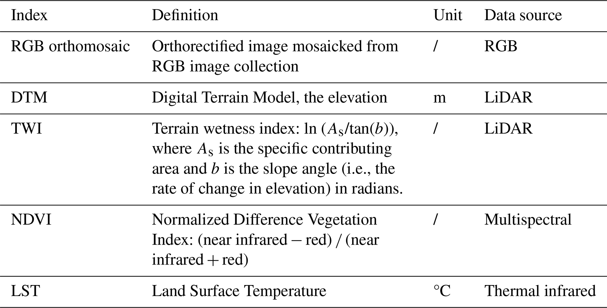
The raw thermal infrared video streams were converted into RJPG images using ThermoViewer version 3.0.26 (TeAX, Arnsberg, Germany). Subsequently, the thermal images were processed with the Pix4D mapper to generate land surface temperature (LST) maps (resolution: 12 cm). To calibrate the LST of each date (Fig. 2a), we first applied linear regressions of temperature obtained by camera and temperature of 2 targets on the ground (Sect. S1, Fig. S2a) to create a correction formula (Fig. S2b). Next, we mapped the spatial variations of surface emissivity using the classification-based approach (Snyder et al., 1998; Li et al., 2013), based on land cover data from our previous work (Fig. 1b; Li et al., 2024) and emissivity values of each class from literature (Snyder et al., 1998). Finally, we converted the LST to thermal radiance using Planck's law, applied an emissivity-based correction, and then converted the radiance back to obtain calibrated LST.

2.7 Daily soil temperature mapping

The linear mixed-effects model was utilized to predict the spatial distribution of daily mean soil temperature (10 cm depth) across the landscape from 1 May 2023 to 30 April 2024. This is because mixed models integrate both fixed and random effects, which provide a robust framework for analyzing data with non-independent structures (Pinheiro and Bates, 2000). Daily mean air temperature, Normalized Difference Vegetation Index (NDVI) and calibrated Land Surface Temperature (LST) were considered as fixed-effect predictors and monitoring sites were included as random effects. The model was performed in RStudio (v4.1.2) using the lmer function of the lme4 package (https://CRAN.R-project.org/package=lme4, last access: 2 September 2025) and was defined as:

$$\begin{array}{}\text{(1)}& y_{ij}={\mathit{\beta }}_{\mathrm{0}}+{\mathit{\beta }}_{\mathrm{1}}{x}_{ij}+\mathrm{\dots }+{\mathit{\beta }}_p{x}_{ij}+b_{\mathrm{0}j}+b_{\mathrm{1}j}{z}_{ij}+\mathrm{\dots }+{\mathit{ϵ}}_{ij}\end{array}$$

Where:

• y_ij is the dependent variable (i.e., soil temperature at 10 cm, unit: °C) for observations i in group j.

• β₀, β₁, …, β_p are fixed-effect coefficients.

• x_ij indicates fixed-effect predictors (independent variables).

• b_0j, b_1j, … are random-effect coefficients associated with group j, which account for variability across groups.

• z_ij indicates predictors associated with random effects.

• ϵ_ij is the residual error term.

Soil temperature data were collected from both Teros 12 sensors and data loggers, as described in Sect. 2.3. Air temperature measurements were obtained from five stations positioned at different slope locations. The NDVI and calibrated LST estimates were extracted from maps by retrieving values at the 20 soil temperature sensor sites (Fig. 1a). These sites were included as random effects in the model to account for repeated measurements at the same locations throughout the monitoring period. For mapping purposes, daily air temperature was statistically downscaled by incorporating the relationship between daily air temperature and elevation, followed by downscaling using a Digital Terrain Model (DTM) derived from LiDAR data (Fig. 2a). The daily NDVI and LST maps were generated by linearly interpolating the monthly/biweekly maps derived from UAVs. The workflow of soil temperature mapping is illustrated in Fig. 2a.

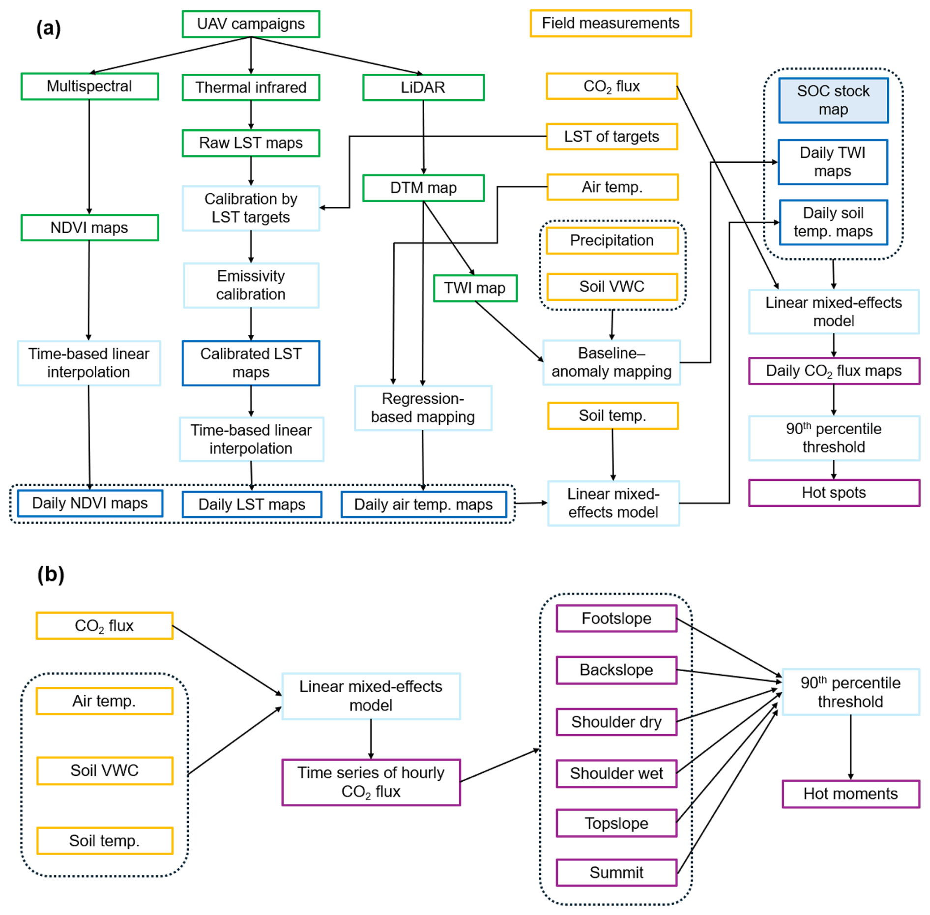
Figure 2 Workflow diagram of daily daytime CO₂ flux spatial mapping (a) and hourly CO₂ flux temporal modeling (b).

2.8 Generation of corrected daily TWI

We generated corrected daily TWI maps to approximate the spatial distribution of daily soil volumetric water content (VWC) by incorporating both long-term site characteristics and daily precipitation effects (Fig. 2a). First, we calculated the mean VWC for each site over the period from 1 May 2023 to 30 April 2024. Then, we extracted each site's TWI values from a TWI map generated using the formula in Table 1. Next, we performed a linear regression with mean VWC as the response and TWI as the predictor:

$$\begin{array}{}\text{(2)}& \text{Baseline}=\text{MeanVWC}=b+a\cdot \text{TWI}\end{array}$$

The “Baseline” represents the soil moisture level at long-term. A baseline map was then created using this regression model. Daily deviations (anomalies) from the baseline were defined as:

$$\begin{array}{}\text{(3)}& {\text{Anomaly}}_t={\text{VWC}}_t-\text{Baseline}\end{array}$$

Considering the memory and lag effects in soil moisture dynamics, we assumed that the anomaly on any day is influenced by the previous day's anomaly and precipitation:

$$\begin{array}{}\text{(4)}& {\text{Anomaly}}_t=c\cdot {\text{Anomaly}}_{t-\mathrm{1}}-d\cdot {\text{Precipitation}}_{t-\mathrm{1}}\end{array}$$

Finally, we generated a “corrected TWI” map for each day by adding the dynamically updated anomaly to the baseline map:

$$\begin{array}{}\text{(5)}& {\text{Corrected TWI}}_t\text{ map}=\text{Baseline map}+{\text{Anomaly}}_t\end{array}$$

This approach allows the daily corrected TWI maps to capture both the inherent spatial variability (as determined by TWI) and the dynamic influence of rainfall, thereby serving as a proxy for the spatial distribution of soil moisture.

2.9 Statistical analysis

All data analyses were conducted in RStudio (v4.1.2). All timestamps in this study were converted to Coordinated Universal Time (UTC) to ensure consistency across datasets. Group differences were assessed by the Kruskal-Wallis test, a non-parametric alternative to the one-way analysis of variance, and suitable for non-normally distributed data (Dunn, 1964). When the Kruskal-Wallis test detected a significant overall effect (p<0.05), Dunn's post-hoc test was performed to determine which groups differed significantly from each other. Pearson correlation analysis was performed using the corrplot package (Murdoch and Chow, 1996). The linear mixed-effects models used to identify factors controlling spatial- temporal variations of CO₂ flux, as well as time series simulation and mapping are introduced below.

2.9.1 Models to explain spatiotemporal variations in CO₂ flux

We also utilized linear mixed-effects modeling framework (i.e., as shown in Sect. 2.7) to assess the impacts of both static and dynamic environmental factors on the spatial and seasonal variability of CO₂ fluxes. Unlike the soil temperature model, the natural logarithm of CO₂ flux observations was utilized as a response. The CO₂ fluxes data are often characterized by extreme values and right-skewed distribution, and a lognormal assumption for CO₂ fluxes could better account for the influences of extreme values on the overall distribution (Wutzler et al., 2020). The fixed-effect predictors were categorized into three groups:

• Static variables: SOC stock, and the ratio of SOC content to nitrogen content ($\mathrm{C}/\mathrm{N}$ ratio).

• Semi-dynamic variables: root biomass and NDVI.

• Dynamic variables: soil temperature and soil moisture at 0–10 cm depth, as well as water table and atmospheric pressure (the latter two variables are shown in the Supplement).

Estimates for NDVI were extracted from the NDVI maps by retrieving the value of the 33 CO₂ flux observation sites and the SOC stock values were extracted from the a local high resolution (0.15 m) SOC stock map (Li et al., 2024). The sites were included as random effects in the seasonal pattern model to account for repeated measurements at the same locations during the monitoring period, whereas slope positions were treated as random effects in the spatial pattern model.

2.9.2 Modelling hourly CO₂ flux

The mixed-effects model was utilized to simulate the time series of CO₂ fluxes at different slope positions (Fig. 2b). Here, the slope position was included as random variable, and the natural logarithm of CO₂ flux (hourly) was set as a response. We utilized CO₂ fluxes data measured by both the LI8100A system and eosFD probes. Specifically, we randomly selected a number of 30 observations from the eosFD probes at each slope position to reduce data redundancy from high-frequency sampling. Afterwards, we applied weighting to adjust the remaining imbalance in data density between the high-frequency eosFD monitoring and low-frequency LI8100A measurements, ensuring both data sources contributed proportionally to the model. The independent variables included hourly soil temperature (10 cm depth), volumetric soil moisture (VWC, 10 cm depth), and air temperature (1.4 m height), considering their importance in explaining the seasonal and diurnal patterns of CO₂ flux. We made simulations of the time series of hourly CO₂ flux for different slope positions from 1 May 2023 to 30 April 2024. Furthermore, we identified CO₂ emission hot moments based on the description in Sect. 2.9.4.

2.9.3 Mapping daily daytime CO₂ flux

The linear mixed-effects model was utilized to map the spatial distribution of daily daytime CO₂ fluxes across the landscape, with daily soil temperature (10 cm depth), corrected daily TWI, and SOC stock being considered as fixed-effect variables and gas sampling sites being included as random variables (Fig. 2a). We predicted the daily daytime CO₂ flux of the landscape from 1 May 2023 to 30 April 2024. Additionally, we calculated the mean daily soil CO₂ flux maps for each season and the entire year. Based on these predictions, we identified hot spots for each day by the methods described below.

2.9.4 Quantifying hot moments and hot spots of CO₂ flux

In previous studies, percentiles have been used as thresholds for identifying heat waves (e.g., Meehl and Tebaldi, 2004: 97.5th percentile), soil heat extremes (e.g., García-García et al., 2023: 90th percentile), hot spots of N₂O emissions (e.g., Mason et al., 2017: median plus three times the interquartile range), and hot spots of CO₂ emissions (e.g., Gachibu Wangari et al., 2023: median plus the interquartile range). In this study, we tested different methods and selected the 90th percentile as the threshold of both hot moments and hot spots to balance capturing extreme CO₂ emissions while maintaining a sufficient sample size. To capture the hot moments, we calculated a threshold for each slope position separately using its own dataset (Fig. 2b). For hot spots, we determined a daily threshold based on each map (Fig. 2a).

2.10 Model performance evaluation

Independent variable coefficients, Intraclass Correlation Coefficient (ICC), coefficients of determination (marginal R² and conditional R²), Root Mean Square Error (RMSE), and Akaike Information Criterion (AIC) were extracted using the modelsummary package after running each model described in Sect. 2.7 and 2.9.1. The ICC quantifies the proportion of variance explained by a grouping (random) factor in multilevel data; values close to 1 indicate high similarity within groups, while values near 0 suggest that grouping conveys little to no information (Nakagawa et al., 2017; Shrout and Fleiss, 1979). The marginal R² represents the variance explained by fixed effects alone, and the conditional R² represents the variance explained by both fixed and random effects (Pinheiro and Bates, 2000). The Kling-Gupta Efficiency (KGE) between observations and predictions was also calculated, with values closer to 1 indicating good model performance (Gupta et al., 2009). The relative importance of each predictor was obtained using the glmm.hp package (Lai et al., 2023, 2022). To assess multicollinearity in regression analysis, the car package was used to calculate the variance inflation factor (VIF) (Fox and Monette, 1992).

For modelling daily soil temperature (i.e., Sect. 2.7) and daily/hourly CO₂ flux (i.e., Sect. 2.9.2 and 2.9.3), we divided the corresponding dataset into a training set (70 %) and a test set (30 %) using K-means clustering, following the methodology of our previous work (Li et al., 2024), to minimize biases that could arise from random sampling (Hair et al., 2010). The models were trained on the training set, and the simulation accuracy was validated using the test dataset. The coefficient of determination (R²), RMSE and KGE were used to assess the quality of all model fits. The daily soil temperature model yielded R², RMSE, and KGE values of 0.89, 1.33 °C, and 0.94, respectively (Fig. S2c, d). Detailed results on model coefficients and performance are summarised in Table S1.

3 Results

3.1 Peat soil surface and subsurface properties

Table 2 presents an overview of soil surface and subsurface properties at different slope positions. The air temperature above ground ∼1.4 m shows great temporal variability, ranging from −8.76 to 24.79 °C within one year. Soil temperatures have smaller temporal variations (0.75–17.48 °C), while the mean daily soil temperature (± one standard deviation (SD)) at the topslope (8.86±3.69 °C) is relatively lower than at other positions. Soil volumetric water content (VWC) across the landscape also exhibits significant spatial heterogeneity. The backslope has the highest mean daily VWC (0.94±0.04 cm³ cm⁻³), followed by the footslope (0.86±0.06 cm³ cm⁻³), shoulder wet (0.85±0.01 cm³ cm⁻³), and summit (0.82±0.04 cm³ cm⁻³). The water table at the topslope showed large fluctuations throughout the year (range: −77.41–0.38 cm; mean ± SD: $-\mathrm{21.76}\pm \mathrm{25.17}$ cm), as shown in Table 2. In contrast, the water table at the shoulder wet slope position remained close to the surface and relatively stable within one year (range: −20.21–4.17 cm; mean ± SD: $-\mathrm{2.17}\pm \mathrm{5.62}$ cm). No significant differences in dry root biomass were observed among the various slope positions, which may be attributed to substantial small-scale variations within each position, particularly at the shoulder, where the biomass ranged from 0.70 to 8.46 g per 100 g soil. The SOC content values for summit and shoulder wet areas are 47.38±2.06 g per 100 g and 47.00±1.41 g per 100 g, respectively. The SOC content in the shoulder and backslope positions is similar, approximately 42 g per 100 g, while the carbon content in the footslope and topslope positions is comparatively lower. In addition, the TN content at the topslope (1.61±0.48 g per 100 g) is significantly lower than at other positions (p<0.05). The $\mathrm{C}/\mathrm{N}$ ratio at the footslope (17.41±1.57) was significantly lower than at the summit, topslope, and backslope (p<0.05), while no significant differences in $\mathrm{C}/\mathrm{N}$ ratios were observed among the other places.

Table 2 Summary of the mean daily air temperature (Air temp.), soil temperature (Soil temp.), soil volumetric water content (VWC), and water table in one year at different slope positions. Soil subsurface properties at 10 cm depth, i.e, dry root biomass, soil organic carbon (SOC) content, total nitrogen (TN) content, and $\mathrm{C}/\mathrm{N}$ ratio, at different slope positions.

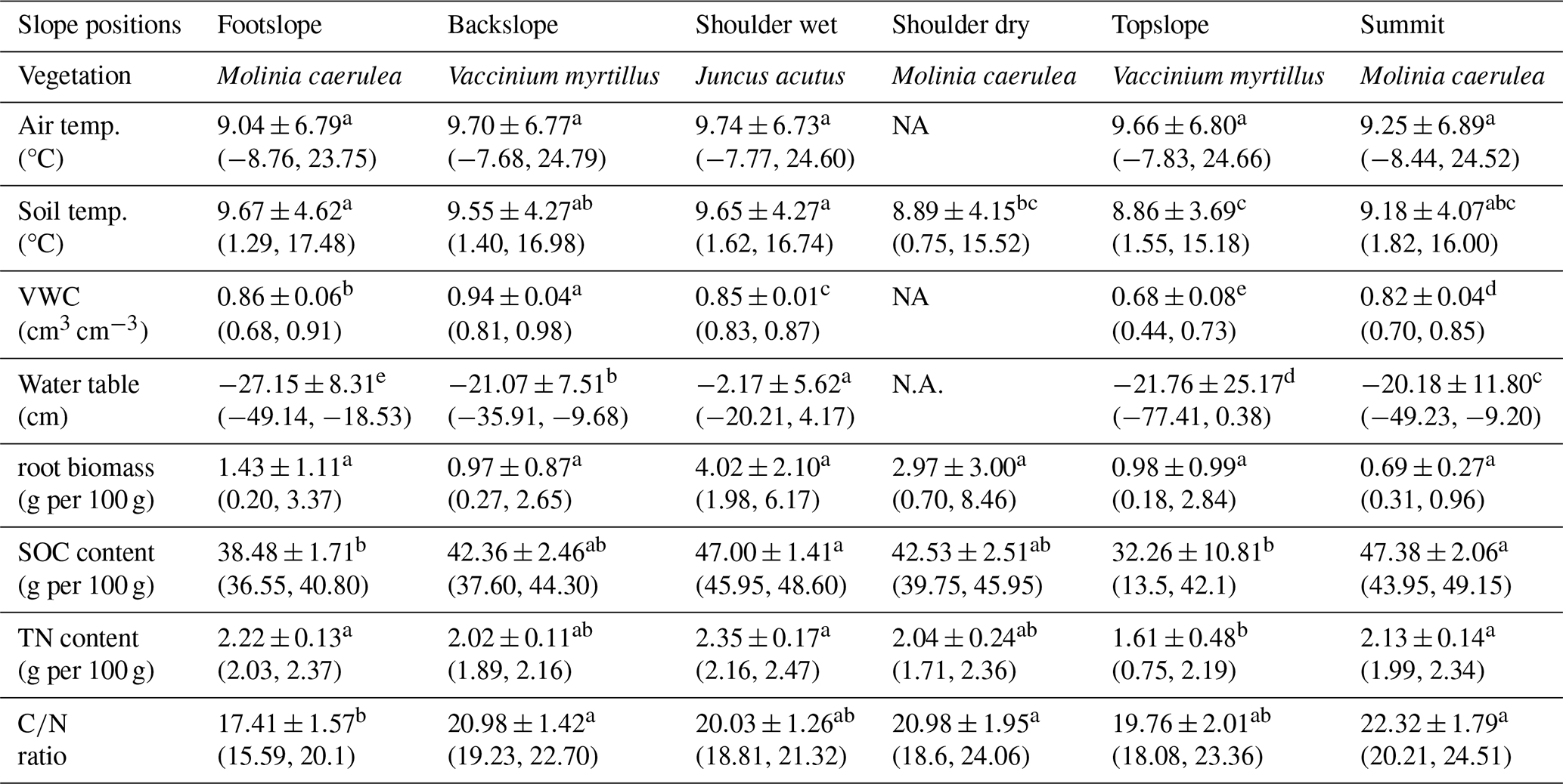
Note: The air temperature was monitored at a height of ∼1.4 m above the ground. The soil temperature and VWC were monitored at a depth of 10 cm by Teros12 sensors. The results are presented as the mean ± one standard deviation (SD) and values in brackets indicate the minimum and maximum values. The Kruskal-Wallis and Dunn's tests were conducted within each class with different superscript letters (a–e) indicating significant differences (p<0.05). NA: not available.

3.2 Spatiotemporal patterns of CO₂ flux

During the monitoring period, the CO₂ emissions show large spatial and seasonal variations across the landscape. The CO₂ fluxes at the footslope (1.25±1.00 $\mathrm{\mu }\mathrm{mol}{\mathrm{m}}^{-\mathrm{2}}{\mathrm{s}}^{-\mathrm{1}}$) and backslope (1.11±1.03 $\mathrm{\mu }\mathrm{mol}{\mathrm{m}}^{-\mathrm{2}}{\mathrm{s}}^{-\mathrm{1}}$) were significantly lower than that of other slope positions (p<0.05) (Fig. 3a). Furthermore, significant differences were observed when grouping the data into three vegetation covers: CO₂ emissions from Vaccinium myrtillus were lower than those from Juncus acutus, with mean ± SD values of 1.59±1.43 and 2.33±2.36 $\mathrm{\mu }\mathrm{mol}{\mathrm{m}}^{-\mathrm{2}}{\mathrm{s}}^{-\mathrm{1}}$, respectively (Fig. 3b) (p<0.05). However, the CO₂ fluxes under Molinia caerulea displayed large variations (0.02–20.1 $\mathrm{\mu }\mathrm{mol}{\mathrm{m}}^{-\mathrm{2}}{\mathrm{s}}^{-\mathrm{1}}$), and no significant differences were found compared to the other two vegetation types. The CO₂ flux data indicated large CO₂ emissions from June to September (3.65±2.68 $\mathrm{\mu }\mathrm{mol}{\mathrm{m}}^{-\mathrm{2}}{\mathrm{s}}^{-\mathrm{1}}$), which can be 8.11 times higher than that from winter and early spring (0.45±0.40 $\mathrm{\mu }\mathrm{mol}{\mathrm{m}}^{-\mathrm{2}}{\mathrm{s}}^{-\mathrm{1}}$) (Fig. 3c). CO₂ emissions in May and October were at a moderate level.

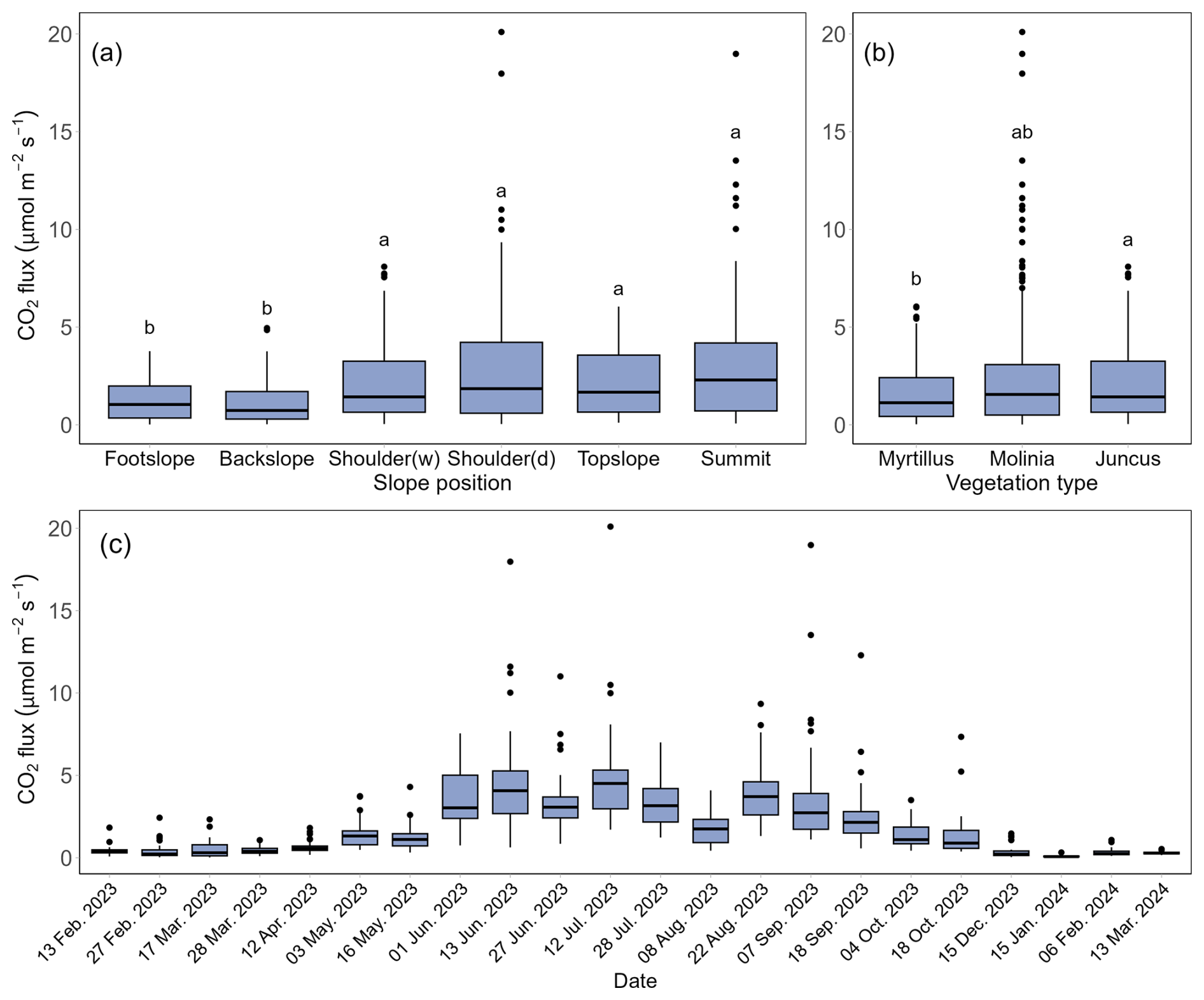
Figure 3 Boxplot of CO₂ flux ($\mathrm{\mu }\mathrm{mol}{\mathrm{m}}^{-\mathrm{2}}{\mathrm{s}}^{-\mathrm{1}}$) across different slope positions (a), vegetation types (b), and sampling dates (c), using data from the LI8100 A system recorded between 13 February 2023 and 13 March 2024. (a) CO₂ flux data of each box were from all dates, and Shoulder (w) and Shoulder (d) indicate shoulder wet and shoulder dry areas, respectively. (b) CO₂ flux data of each box were from all dates, and Myrtillus, Molinia and Juncus indicate Vaccinium myrtillus, Molinia caerulea and Juncus acutus, respectively. (c) CO₂ flux data of each box were from all slope positions. The edges of each box represent the first quartile (Q1) and third quartile (Q3), while the line inside the box indicates the median CO₂ flux. Whiskers extend from the box to the smallest and largest values within 1.5 times the interquartile range, and points outside the whiskers are considered extreme values. The Kruskal-Wallis and Dunn's tests were performed within slope positions and vegetation types, with different letters indicating significant differences among groups (p<0.05).

At the daily scale, the soil respiration displayed a clear diurnal trend from April to August (Fig. S3), particularly at the footslope (Fig. S3a), backslope (Fig. S3b), and shoulder (Fig. S3c, d) slope positions, with higher CO₂ emissions observed in the late afternoon (14:00–18:00) and lower emissions in the morning (04:00–08:00). In contrast, the diurnal trend of CO₂ flux at the topslope (Fig. S3e) and summit (Fig. S3f) in autumn was less pronounced. Figure 4a presents examples of time series data for CO₂ fluxes and environmental factors at the footslope, topslope, and summit from August to October 2024. In August, clear diurnal patterns with variation magnitudes of 2–3 $\mathrm{\mu }\mathrm{mol}{\mathrm{m}}^{-\mathrm{2}}{\mathrm{s}}^{-\mathrm{1}}$, and reduced CO₂ emissions following precipitation events on 13 August and 17 August were observed at the footslope (Fig. 4a, b). Since the middle of September, the diurnal variation was less than 1 $\mathrm{\mu }\mathrm{mol}{\mathrm{m}}^{-\mathrm{2}}{\mathrm{s}}^{-\mathrm{1}}$ and there was no obvious pattern in daily changes (Fig. 4a, c).

3.3 Factors contributing to spatiotemporal variability

Three types of environmental factors explain 64 % of the observed seasonal variance in CO₂ emissions, with contributions of 33 % from soil temperature, 10 % from VWC, 19 % from vegetation (i.e., NDVI, root biomass), 2 % from relatively static factors (i.e., SOC stock, $\mathrm{C}/\mathrm{N}$ ratio), and 6 % from random effects (i.e., 33 sampling sites) (Table 3). This suggests that long-term stable environmental factors have minimal direct influence on seasonal CO₂ flux patterns. Interestingly, the contribution of these relatively stable factors is nearly 6 times higher in explaining overall spatial variations, although soil temperature is still the dominant factor (Table 3). The low ICC values in both spatial and seasonal models highlight significant small-scale heterogeneity in soil respiration. Water table contributed 10 % of seasonal variation and atmospheric pressure was not important (1 %), as shown in Table S2 of the Supplement. The relationships between each environmental factor and CO₂ fluxes are shown in Fig. S4.

Table 3 Coefficients and relative contributions of three types of input variables (static, semi-dynamic, dynamic) of mixed linear regression models for modelling CO₂ flux. Random effects were evaluated by ICC and model performance was evaluated by Marginal R², Conditional R², AIC, RMSE, and KGE.

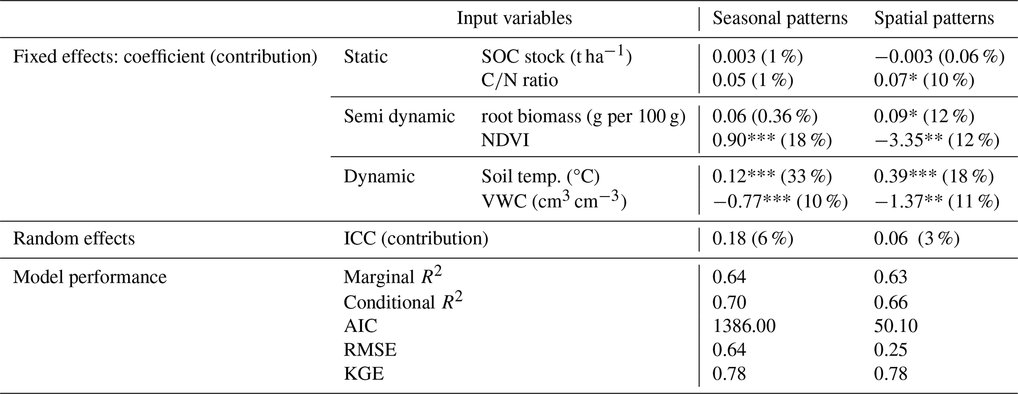
Note: Significance level: *** p<0.001, ** p<0.01, * p<0.05. All CO₂ fluxes (unit: $\mathrm{\mu }\mathrm{mol}{\mathrm{m}}^{-\mathrm{2}}{\mathrm{s}}^{-\mathrm{1}}$), soil temperature, and VWC data for spatial and seasonal patterns were from the LI8100 A system. To investigate the factors controlling spatial variations of CO₂ flux, we calculated the mean values of CO₂ flux, NDVI, soil temperature, and VWC of each site during the monitoring time.

3.4 Continuous hourly time series of CO₂ flux and hot moments

Three dynamic variables (i.e., soil temp., VWC, air temp.) were taken into account to predict the time series of hourly CO₂ flux at different slope positions. These input variables were selected due to their influential roles in explaining the diurnal (Figs. S3, 4) and seasonal (Table 3) fluctuations of CO₂ emissions. As shown in Table 4, the temporal model yielded a robust performance in both training and testing dataset, achieving R², RMSE, and KGE values of 0.86,0.39 $\mathrm{\mu }\mathrm{mol}{\mathrm{m}}^{-\mathrm{2}}{\mathrm{s}}^{-\mathrm{1}}$, 0.90, and 0.74, 0.57 $\mathrm{\mu }\mathrm{mol}{\mathrm{m}}^{-\mathrm{2}}{\mathrm{s}}^{-\mathrm{1}}$, 0.77, respectively.

Table 4 Model performance for simulating time series of hourly CO₂ flux ($\mathrm{\mu }\mathrm{mol}{\mathrm{m}}^{-\mathrm{2}}{\mathrm{s}}^{-\mathrm{1}}$) and mapping daily daytime CO₂ flux ($\mathrm{\mu }\mathrm{mol}{\mathrm{m}}^{-\mathrm{2}}{\mathrm{s}}^{-\mathrm{1}}$) across the landscape.

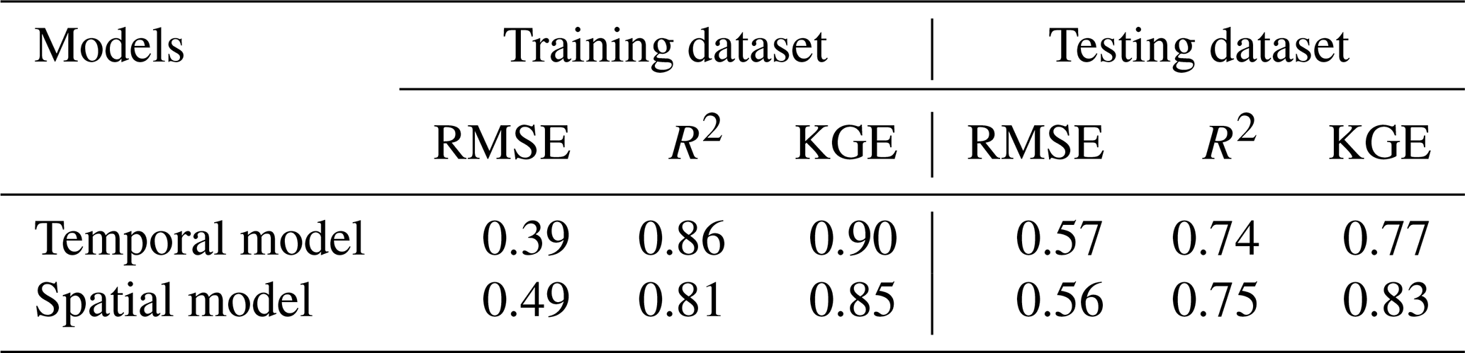
Note: Temporal model used the natural logarithm of CO₂ flux data from LI8100 A and eosFD probes, whereas spatial model used the natural logarithm of CO₂ flux data only from LI8100 A.

Table 5 Summary of modelled mean ± SD CO₂ fluxes, thresholds for identifying hot moments, total CO₂ flux, and the contribution of hot moments to total flux at different slope positions.

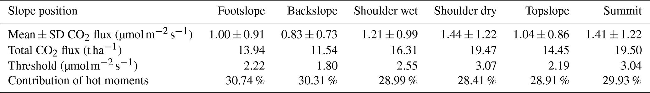
The modelled CO₂ emissions at all slope positions display a clear seasonal trend, with higher CO₂ fluxes from June to September and lower estimates in other months, in line with the observed fluxes shown in brown dots (Fig. 5d–i). The total CO₂ fluxes (Table 5) at the summit (19.50 t ha⁻¹) and the shoulder (dry: 19.47 t ha⁻¹, wet: 16.31 t ha⁻¹) slope positions were higher than that of topslope (14.45 t ha⁻¹), followed by footslope (13.94 t ha⁻¹) and backslope (11.54 t ha⁻¹), consistent with the spatial patterns of our observations (Fig. 3a). Most hot moments occurred from June to September 2023, whereas few hot moments were observed from late July to the early August (Fig. 5d–i). Although these hot moments of different slope positions only accounted for 10 % across the year, they could contribute 28 %–31 % to the annual total CO₂ emissions (Table 5).

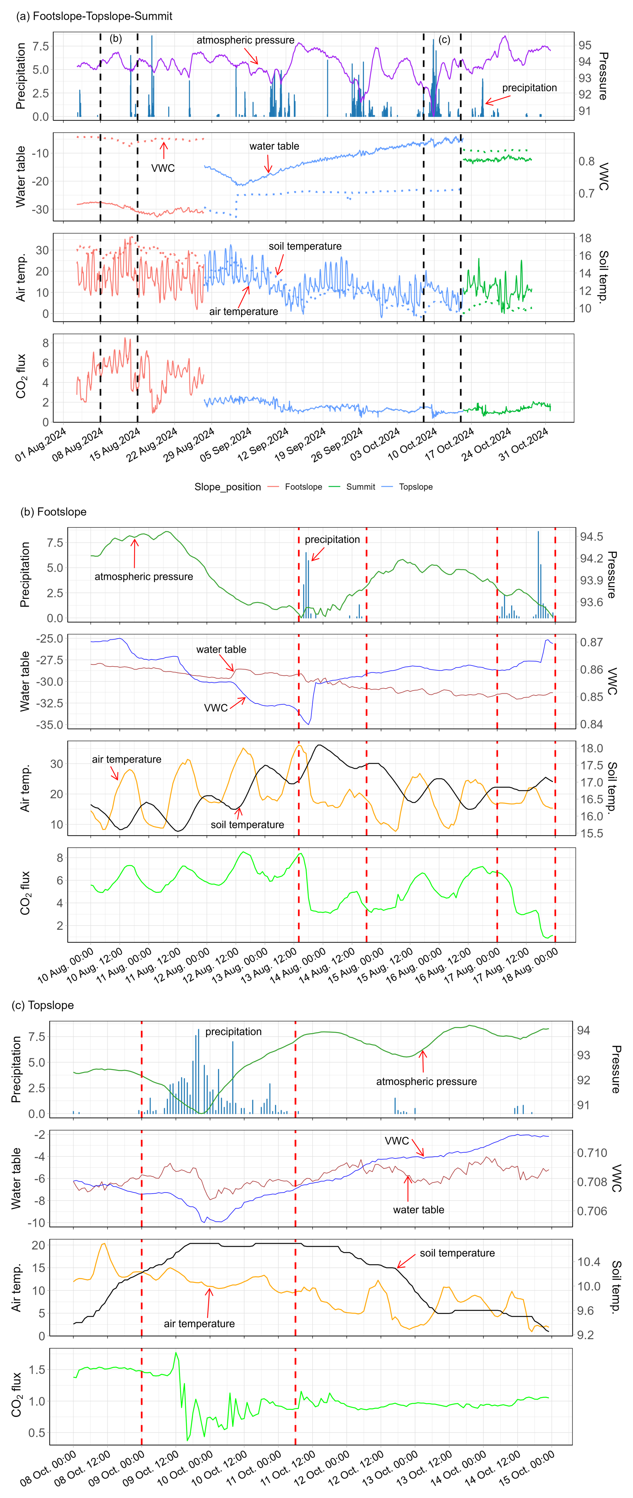
Figure 4 Examples showing time series data of air pressure (kPa), precipitation (mm), soil volumetric water content (VWC, cm³ cm⁻³), water table (cm), soil temperature (Soil temp., °C), air temperature (Air temp., °C), and CO₂ flux ($\mathrm{\mu }\mathrm{mol}{\mathrm{m}}^{-\mathrm{2}}{\mathrm{s}}^{-\mathrm{1}}$, measured by eosFD probes) from 1 August 2024 to 31 October 2024 (a), from 8 August 2024 to 15 August 2024 at the footslope (b), and from 8 October 2024 to 15 October 2024 at the topslope slope position (c). The black vertical dashed lines in panel (a) indicate the two periods shown in panels (b) and (c). The red vertical dashed lines in panels (b) and (c) indicate the precipitation events.

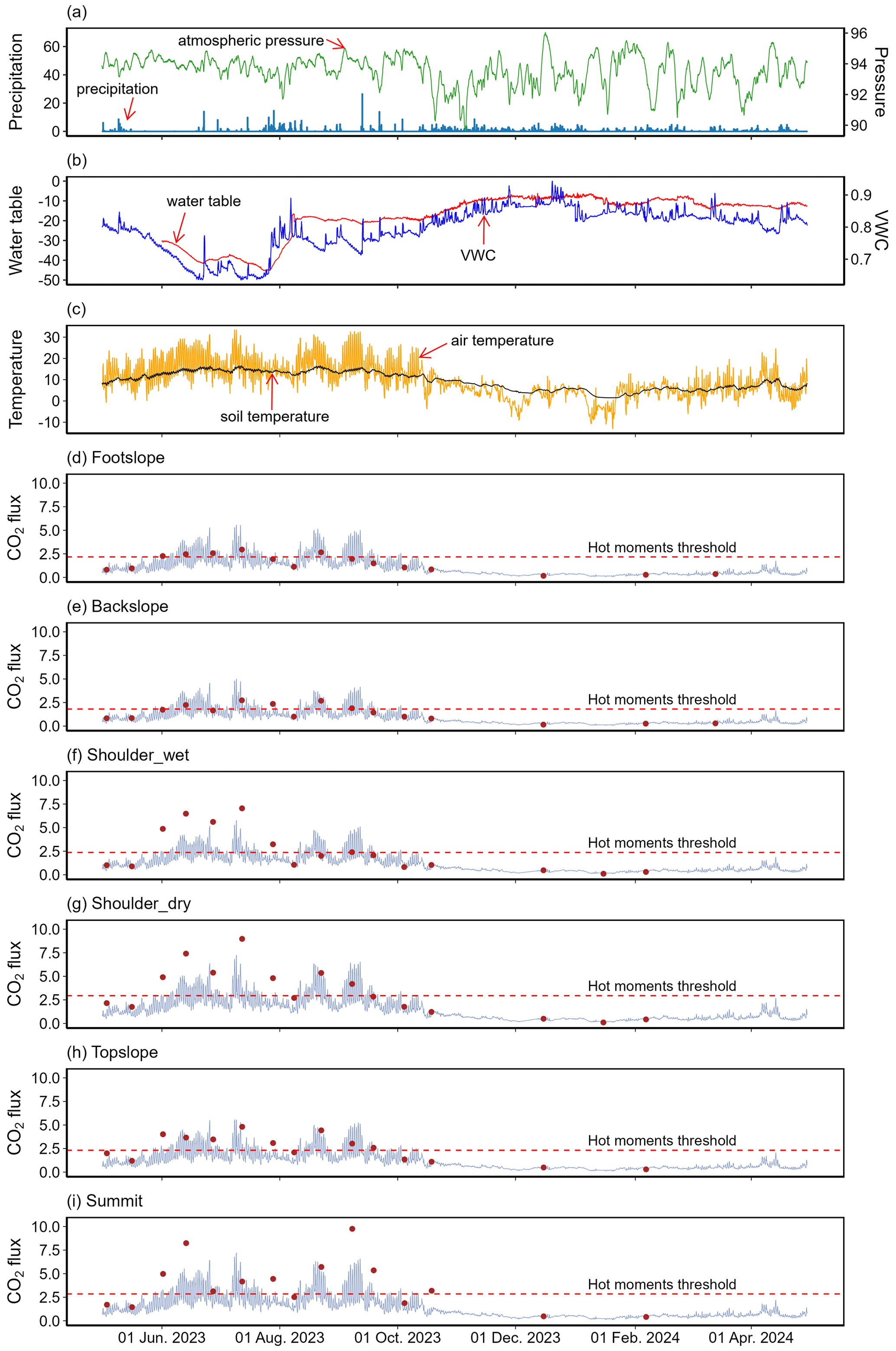
Figure 5 Time series of hourly precipitation (blue bar) and atmospheric pressure (light green line) (a), hourly mean VWC (blue line) and water table (red line) (b), hourly mean air temperature (orange line) and soil temperature (black line) (c), modelled hourly CO₂ flux (purple lines) and in-situ measurements (brown dots) at different slope positions (d–i). Precipitation (mm) and atmospheric pressure (kPa) data was from the nearby meteorological observation station (50.51° N, 6.07° E). The water table (cm) data were derived from the Solinist probes. The VWC (cm³ cm⁻³) and soil temperature (°C) were mean values from five slope positions monitored by Teros12 sensors at a depth of 10 cm. Air temperatures (°C) were mean values from 5 stations at 1.4 m height above ground. Measured CO₂ fluxes ($\mathrm{\mu }\mathrm{mol}{\mathrm{m}}^{-\mathrm{2}}{\mathrm{s}}^{-\mathrm{1}}$) were from the LI8100A system.

3.5 Daily daytime CO₂ flux maps and hot spots

A linear mixed-effects model was utilized to map daily daytime CO₂ flux from 1 May 2023 to 30 April 2024, incorporating soil temperature, corrected TWI, and SOC stock as predictors due to their significant role in explaining the spatial-seasonal variability of CO₂ flux and their availability as spatial data. The mapping model yielded robust performance metrics (Table 4), with R², RMSE, and KGE values of 0.81, 0.49 $\mathrm{\mu }\mathrm{mol}{\mathrm{m}}^{-\mathrm{2}}{\mathrm{s}}^{-\mathrm{1}}$, and 0.85 in the training dataset, and 0.75, 0.56 $\mathrm{\mu }\mathrm{mol}{\mathrm{m}}^{-\mathrm{2}}{\mathrm{s}}^{-\mathrm{1}}$, and 0.83 in the test dataset, respectively.

Consistent with our observations, the modelled soil respiration also displayed substantial spatiotemporal heterogeneity (Fig. 6a–d). More specifically, the mean CO₂ fluxes ranged from 0.09 to 8.23 $\mathrm{\mu }\mathrm{mol}{\mathrm{m}}^{-\mathrm{2}}{\mathrm{s}}^{-\mathrm{1}}$ in spring (Fig. 6a), 0.31 to 33.83 $\mathrm{\mu }\mathrm{mol}{\mathrm{m}}^{-\mathrm{2}}{\mathrm{s}}^{-\mathrm{1}}$ in summer (Fig. 6b), 0.15 to 16.88 $\mathrm{\mu }\mathrm{mol}{\mathrm{m}}^{-\mathrm{2}}{\mathrm{s}}^{-\mathrm{1}}$ in autumn (Fig. 6c), and 0.03 to 2.47 $\mathrm{\mu }\mathrm{mol}{\mathrm{m}}^{-\mathrm{2}}{\mathrm{s}}^{-\mathrm{1}}$ in winter (Fig. 6d). Many modelled mean CO₂ fluxes at the footslope and backslope (elevation <660 m) remained below 2 $\mathrm{\mu }\mathrm{mol}{\mathrm{m}}^{-\mathrm{2}}{\mathrm{s}}^{-\mathrm{1}}$ (Fig. 6e). In contrast, the modelled CO₂ emissions remained higher throughout the year at the shoulder (660 m ≤ elevation ≤ 670 m) and east of summit (elevation >675 m) with high vegetation cover (Fig. 1b). About 10 % of the area were identified as hot spots, with a high frequency of hot spots occurring in these regions, while the locations of sporadic hot spots varied over time (Fig. 6f). Overall, the landscape emitted approximately 12.41 t ha⁻¹ CO₂ to the atmosphere during the simulation period, with 20.41±0.61 % of the CO₂ fluxes coming from the hot spots.

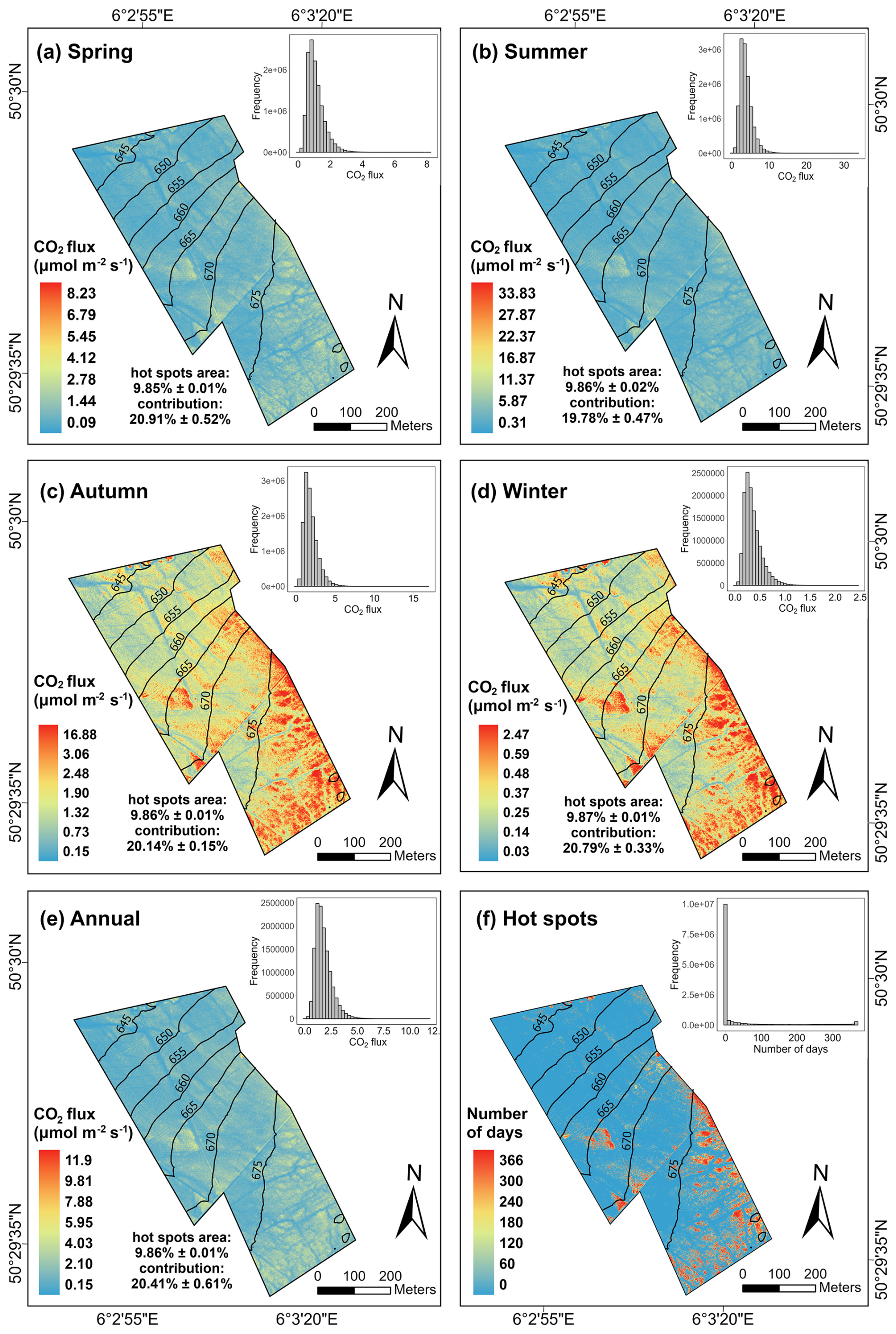
Figure 6 Maps of modelled mean daily daytime CO₂ flux ($\mathrm{\mu }\mathrm{mol}{\mathrm{m}}^{-\mathrm{2}}{\mathrm{s}}^{-\mathrm{1}}$) in four seasons (a, b, c, d), throughout the year (e), and hot spot frequency (f). To enhance contrast, all maps were visualized with a display stretch based on 2± standard deviations in ArcGIS Pro. The histograms of pixel values are presented on the top-right corner of each map. The hot spots area proportion and CO₂ flux contribution from the hot spots of each season and across the year are summarized in the corresponding maps.

4 Discussion

4.1 Drivers of spatiotemporal heterogeneity in CO₂ emission

Consistent with prior temperate peatland studies (Juszczak et al., 2013; Wilson et al., 2015; Danevčič et al., 2010; Swails et al., 2022), our results indicate that seasonal variations in soil CO₂ flux across the landscape are highly related to soil temperature, which could account for 33 % of the seasonal variability (Table 3). This relationship is likely due to the influence of temperature on microbial activity, as well as the distinct seasonal patterns in temperature observed in our study (Fig. 5c), which in turn drive corresponding fluctuations in soil respiration throughout the year (Fig. 3c). Moreover, spatial heterogeneity in soil temperature further shaped landscape-scale CO₂ emission patterns (Table 3). For instance, the south-facing summit slopes, which receive more solar radiation in the daytime, consistently show higher CO₂ fluxes (Fig. 3a). Conversely, the north-facing footslope and backslope, situated on the windward side, experience lower temperatures, resulting in generally lower soil respiration rates throughout the observation period (Fig. 3a). At the daily scale, clear soil temperature oscillations were observed in the surface peat, while these diurnal cycles were damped and delayed with depth, with temperature peaks typically occurring at night and valleys around midday (Figs. 4, S3). In contrast, the diurnal pattern of soil respiration during growing season (i.e., April to August; Figs. 4, S3) was more closely aligned with air temperature, highlighting the important role of air temperature in regulating short-term variations in soil respiration.

Soil water content influences oxygen availability and nutrients transport within the peat profile, thereby regulating microbial decomposition, plant root activity, and ultimately CO₂ production (Hatala et al., 2012; Knox et al., 2015; Zou et al., 2022; Huang et al., 2021; Deshmukh et al., 2021). Previous studies reported nonlinear relationships between soil moisture and soil respiration (Kechavarzi et al., 2010; Marwanto and Agus, 2014; Wood et al., 2013), as both excessively dry and overly saturated conditions can limit microbial decomposition. In our study case, we observed a negative correlation between soil volumetric water content (VWC) and CO₂ fluxes (Table 3, Fig. S4), with VWC explaining approximately 10 % of the spatial and seasonal variability in soil respiration (Table 3). This may partially explain the slightly higher CO₂ fluxes in drier shoulder positions compared to wetter areas (Fig. 3a). Numerous studies have demonstrated that water table levels play a crucial role on soil respiration (Berglund and Berglund, 2011; Evans et al., 2021; Hoyt et al., 2019; Knox et al., 2015). For example, Knox et al. (2015) demonstrated that a declining water table caused by drainage increases oxygen penetration into the peat, resulting in higher CO₂ flux compared to restored peatlands. Our study also observed negative correlations between the water table and CO₂ fluxes (Figs. 4a, S4), whereas the water table accounted for only 10 % of CO₂ flux seasonal variations (Table S2). This relatively modest contribution may be attributed to (i) the limited number of observation sites (i.e., 5 sites along the hillslope), (ii) short duration of water table monitoring that matched the CO₂ flux measurement periods, and (iii) the generally low water table throughout the year (Table 2), particularly at the footslope, backslope, and summit, where maximum water tables remained >9 cm below the ground. This maintained aerobic layers that support soil respiration, thereby reducing the influence of water table fluctuations on CO₂ fluxes. Increasing spatial coverage and temporal resolution of water table observations across the landscape would likely improve our ability to examine its influence on CO₂ emissions.

Atmospheric pressure can influence gas fluxes via pressure pumping (Ryan and Law, 2005), and thus we examined its influence on CO₂ emission. However, when atmospheric pressure was included as a predictor in our model, it only accounted for 1 % of seasonal variability in CO₂ fluxes (Table S2). Examination of high-frequency time series data (i.e., hourly CO₂ flux from the eosFD probes) showed that at the daily scale, the diurnal pattern of CO₂ fluxes did not follow atmospheric pressure fluctuation (Fig. 4). At longer time scales, the two variables displayed only weak correlations. Moreover, we observed that declines in atmospheric pressure were often followed by precipitation events, which in turn were associated with decreases in both air temperature and CO₂ flux, or slight CO₂ fluxes increases (Fig. 4). This suggests that atmospheric pressure may indirectly influence soil respiration by affecting precipitation patterns, rather than exerting a strong direct control. In saturated peatlands, falling atmospheric pressure has been shown to trigger methane (CH₄) ebullition by releasing trapped gas bubbles (Tokida et al., 2007, 2005; Baird et al., 2004), while in our study site, which is a hillslope where the surface peat remains aerobic most of the time (Table 2), such bubble formation and ebullition are likely minimal. Another contributing factor maybe the limitations of our observations that may have limited our ability to detect short-lived CO₂ flux responses to atmospheric pressure fluctuations.

Previous studies have shown that vegetation mediates soil respiration through root respiration, exudates, litter inputs, and rhizosphere priming effects (Acosta et al., 2017; Wang et al., 2015a; Walker et al., 2016; Jovani-Sancho et al., 2021; Bragazza et al., 2013). Root respiration, which is closely linked to plant photosynthetic activity, contributes directly to the overall soil CO₂ fluxes (Crow and Wieder, 2005). In our study, the contribution from root biomass becomes more substantial in the spatial model (i.e., 12 %) than in the seasonal model (<1 %, Table 3). This discrepancy is likely because root biomass was measured only once during the entire CO₂ monitoring period, thereby missing its seasonal dynamics. The monthly/biweekly NDVI is the second-most influential predictor for CO₂ seasonal fluctuations (Table 3), explaining 18 % of variability, as NDVI reveals vegetation phenology during the monitoring period. Accordingly, positive correlation was observed between CO₂ flux and NDVI at the seasonal scale (Table 3, Fig. S4). In the spatial-pattern model, however, the annual mean NDVI explained 12 % of the spatial variability in CO₂ fluxes (Table 3) and the relationship became negative ($r=-\mathrm{0.29}$, p=0.11). This shift in correlation may be due to differences in vegetation structure and composition across the landscape. Slope positions with higher mean NDVI values (i.e., topslope and backslope) are mainly covered by dwarf shrubs (i.e., Vaccinium myrtillus), which exhibit lower CO₂ fluxes compared to other vegetation types (Fig. 3b). The lower CO₂ fluxes in dwarf shrub areas are likely associated with their lower root biomass (Table 2). Furthermore, it has been shown that dwarf shrubs in northern peatlands produce high-phenolic litter with higher resistance to breakdown and introduce more water-soluble phenolics into the soil compared to Sphagnum moss/herbs (Bragazza et al., 2013; Wang et al., 2015a), which further constrains microbial activity and CO₂ production. In addition, vegetation cover may indirectly influence soil respiration by regulating surface microclimate conditions such as humidity and temperature (Nichols, 1998; Stoy et al., 2012).

As shown in Table 3, the SOC stock and $\mathrm{C}/\mathrm{N}$ ratio have limited explanatory power for the seasonal variability of CO₂ flux, in line with findings of Danevčič et al. (2010). However, when analyzing drivers of average soil CO₂ flux rate across the entire monitoring period, the importance of $\mathrm{C}/\mathrm{N}$ ratio increased nearly 11 times (Table 3). This likely reflects how long-term averaging integrates short-term dynamic variability, thereby amplifying the role of spatial heterogeneity mediated by the $\mathrm{C}/\mathrm{N}$ ratio. Prior studies suggesting that the quality of organic material, rather than its quantity, primarily regulates CO₂ fluxes in peatlands (Hoyos-Santillan et al., 2016; Leifeld et al., 2012). Specifically, the soil $\mathrm{C}/\mathrm{N}$ ratio is known to regulate microbial community functionality and respiration intensity (Leifeld et al., 2020; Briones et al., 2014; Ishikura et al., 2018; Wang et al., 2015b).

4.2 CO₂ emission hot moments and hot spots: identification, implications, and importance

4.2.1 Temporal analysis and hot moments

During past decades, efforts have been made to model CO₂ flux over time based on its relationship with environmental factors such as hydrology, temperature, substrate quality, microbial community, and vegetation (Hoyt et al., 2019; Junttila et al., 2021; Schubert et al., 2010; Rowson et al., 2012; Abdalla et al., 2014; Farmer et al., 2011; Anthony and Silver, 2021). In our study, diurnal cycles of CO₂ fluxes are closely related to air temperature (Figs. 4, S3), while soil temperature and moisture are important factors in explaining the seasonal patterns of CO₂ flux (Table 3). Hence, the three dynamic environment variables were incorporated into the model to simulate the hourly CO₂ flux across the entire monitoring period. Overall, the temporal model demonstrated robust performance in both the training and testing datasets (Table 4) and effectively captured seasonal and diurnal trends at most sites (Fig. 5d–i). However, the modelled peak values are lower than the observations at shoulder and summit slope positions (Fig. 5g, f, i), which may be partially due to the limited number of high-value observations in these areas. Consequently, the model is more influenced by the more frequent lower CO₂ fluxes, leading to an overall underestimation of the peak. In addition, two types of gas analyzers were employed to monitor CO₂ flux with different sampling frequency and time: the LI-8100A sensor was used biweekly or monthly to capture seasonal trends, while eosFD probes collected data every 5 min to track diurnal fluctuations. The integration of these datasets for modelling temporal dynamics improved estimation accuracy but might also introduce uncertainties into the model.

Anthony and Silver (2023) demonstrated that identifying hot moments of CO₂ flux in peatland requires intensive continuous measurements, while as an alternative, our robust simulation of hourly CO₂ flux enabled the identification of hot moments in a complex landscape. We found that most of these hot moments occurred during the summer and early autumn seasons (Fig. 5d–i), in agreement with our in-situ observations (Fig. 3c). The frequent high CO₂ emissions in June and July can be attributed to the low precipitation and water table level, decreased soil moisture, and high temperatures (Fig. 5a–c). In water-limited ecosystems or during the dry season of tropical peatlands, precipitation pulses can trigger hot moments of CO₂ gas emissions, as precipitation regulates soil moisture and infiltrating water physically displaces CO₂ from soil pores (Fernandez-Bou et al., 2020; Leon et al., 2014; Wright et al., 2013). This occurs when rainwater rapidly infiltrates dry soil, filling air-filled pores and forcing CO₂-rich air out due to hydraulic pressure. In this study, CO₂ fluxes showed both decreases and increases in response to precipitation events (Fig. 4). The observed decreases may be attributed to the high water content of the surface peat, and prolonged and intense rainfall led to lower temperatures, increased soil moisture, and higher water table (Figs. 4, 5b, c), thereby suppressing microbial and root respiration. Consequently, a few hot moments were captured during late July and early August during the heavy rainfall events (Fig. 5). Following this period, CO₂ emissions reached values that exceeded the “hot moments” threshold in mid-August, aligning with declining rainfall and rising temperatures (Fig. 5d–i). The hot moments observed in September are linked to seasonal fluctuations in atmospheric pressure, precipitation, water table, and temperature (Fig. 5a–c).

Similar to the findings of Anthony and Silver (2021) and Kannenberg et al. (2020), these hot moments accounted for approximately 10 % throughout the year, while they contributed significantly to the annual total CO₂ emissions (28 %–31 %; Table 3), highlighting the important role of short-term high-emission events in the overall carbon emission. Therefore, missing hot moments may lead to significant underestimates of total peat soil respiration budgets. Despite continuous automated chamber or eddy covariance measurements that are ideal for capturing hot moments of CO₂ emissions (Anthony and Silver, 2023; Hoyt et al., 2019; Anthony and Silver, 2021), long-term continuous monitoring is still labor-intensive and cost-prohibitive in many locations within the complex peatland ecosystems. Given that we observed a concentration of hot moments in the summer and autumn, we recommend increasing monitoring frequency during these seasons for temperate peatlands. This strategy would help capture carbon emission dynamics more effectively, reduce uncertainties in annual carbon flux estimates, and provide more representative peatland CO₂ flux data.

4.2.2 Spatial analysis of CO₂ fluxes and hot spots

Our mapping of daily daytime CO₂ flux across the landscape yielded a model performance of R²=0.75, KGE = 0.83, and RMSE = 0.56 $\mathrm{\mu }\mathrm{mol}{\mathrm{m}}^{-\mathrm{2}}{\mathrm{s}}^{-\mathrm{1}}$ for the test dataset (Table 4). This can be attributed to the incorporation of key environmental factors that drive the spatiotemporal heterogeneity of soil respiration into the model inputs. These factors – including soil temperature, corrected TWI, and SOC stock – can be estimated using high spatiotemporal resolution UAV data. Previous studies upscaled spatial carbon fluxes using area-weighted methods, extrapolating point data from CO₂ chamber flux measurements to adjacent or larger areas based on land cover maps (van Giersbergen et al., 2024; Webster et al., 2008; Leon et al., 2014). However, this approach can lead to over- or underestimation (Gachibu Wangari et al., 2023; Leifeld and Menichetti, 2018), because our findings reveal that even within the same vegetation cover, such as Molinia caerulea, CO₂ emissions exhibit significant spatiotemporal variability (Fig. 3b). In recent years, spatial upscaling of CO₂ fluxes has increasingly relied on satellite-based remote sensing data (e.g., Junttila et al., 2021; Gachibu Wangari et al., 2023; Zhang et al., 2020; Azevedo et al., 2021; Huang et al., 2015. While this method covers larger areas, it is often constrained by coarse temporal and spatial resolutions. The peatland ecosystem is characterized by great temporal and spatial heterogeneity at small scales, and ignoring these variations can introduce significant uncertainties in CO₂ emission estimates. Our study demonstrates that multi-sensor and multi-date UAV remote sensing has great potential in modeling CO₂ fluxes with high resolution (i.e., spatial: 15 cm; temporal: daily interval), thereby reducing uncertainties in spatiotemporal predictions of CO₂ fluxes.

However, the key environmental variables used for mapping soil respiration were estimated by UAV data, which inevitably introduce uncertainties into the prediction processes. For instance, because daily UAV imagery was unavailable, the predictors (i.e., air temperature, LST, and NDVI) for modelling the spatiotemporal dynamics of soil temperature were linearly interpolated between acquisition dates, potentially adding uncertainty to the model results. Moreover, flight conditions and preprocessing of the raw UAV data (e.g., georeferencing, resampling, the calibration of LST, downscaling air temperature) may have further introduced errors into the soil temperature estimates. The corrected daily TWI maps were also subject to uncertainty, as they relied on in-situ soil VWC observations, which were only available in the middle transect of the landscape. Similarly, uncertainties in SOC stock mapping arose from the peat thickness estimation and soil sampling strategy, as discussed in our previous work (Li et al., 2024). Nevertheless, these reliable high-resolution CO₂ flux maps allowed for the identification of hot spot areas across the landscape. We found that most of the hot spots occurred to the west of shoulder areas and to the east of the summit which is covered by dense vegetation (Figs. 1b, 6f). Some sporadic hot spots were found at the backslope and footslope positions. Spatial variability in the factors controlling biogeochemical processes, such as soil temperature, moisture, water table depth, vegetation type, and substrate quality, is likely driving these differences (Anthony and Silver, 2023; Kuzyakov and Blagodatskaya, 2015; McNamara et al., 2008). For instance, the persistent hot spots that occurred at the shoulder might be due to their relatively drier conditions and higher carbon stocks compared to other areas (Li et al., 2024). The tree-covered areas at the summit likely contribute substantial root respiration, which could sustain hot spot formation throughout the year. Besides, litterfall beneath trees insulates the peat soil and provides an abundant resource for microbial activity even during the non-growing season. While at other places, such as the footslope and backslope, which are mainly covered by dwarf shrubs and Molinia caerulea (Fig. 1b) with pronounced seasonal phenology, they potentially form sporadic soil respiration hot spots at specific times of the year. Furthermore, surface peat beneath relatively short vegetation can receive higher direct solar radiation in summer, leading to elevated soil temperatures and the emergence of carbon emission hot spots.

High-emission events from hot spots play a crucial role in overall CO₂ fluxes (Anthony and Silver, 2023), hence, neglecting these areas could lead to substantial underestimation of peatland carbon emissions. In our study, although less than 10 % of area was identified as hot spots, their CO₂ flux contribution accounted for nearly 20 % across the year (Fig. 6). However, research specifically focusing on peatland CO₂ emission hot spots remains limited (Anthony and Silver, 2023), despite increased exploration of greenhouse gas emission hot spots in other ecosystems (e.g., agricultural field (Krichels and Yang, 2019; Rey-Sanchez et al., 2022; Leifeld et al., 2020); wetland (Rey-Sanchez et al., 2022); water-limited Mediterranean ecosystem (Leon et al., 2014); forest (Gachibu Wangari et al., 2023)). Hence, to improve the accuracy of CO₂ spatial budgeting for peatlands, there is a need for enhanced high-resolution dynamic monitoring of hot spot areas (Becker et al., 2008). Our study demonstrates the great potential of UAV technology for peatland hot spot identification and quantification, offering new insights into studying soil respiration within heterogeneous ecosystems as well as optimizing peatland management and CO₂ emission reduction strategies.

5 Conclusion

In this study, we monitored the dynamics of peatland surface and subsurface environments using both field surveys and multi-sensor UAVs at high spatiotemporal resolution. We investigated the influence of dynamic and static environmental factors on soil respiration rates across different scales, thereby enhancing our understanding of peatland carbon cycling. Additionally, we simulated CO₂ flux with high spatiotemporal resolution by integrating field measurements and UAV data. These reliable modelling allow us to identify and quantify CO₂ emission hot spots and hot moments across the landscape. To summarize, the main findings of our study are as follows:

1. Soil respiration rates vary significantly across space and time, influenced by both dynamic and relatively static environmental factors at different scales. Temperature is the primary driver of CO₂ flux variations, explaining 33 % CO₂ seasonal variability and 18 % spatial variability. Soil moisture negatively affects both seasonal and spatial variations, accounting for 10 %–11 % of the variance. Water table dynamics also play a role (10 %), but more observations are needed to explore its influence. Atmospheric pressure may indirectly influence soil respiration by affecting precipitation patterns, rather than exerting a strong direct control. Semi-dynamic factors (i.e., NDVI and root biomass) contribute 19 % to seasonal variability and 24 % to spatial variability. While relative static factors (i.e., the $\mathrm{C}/\mathrm{N}$ and SOC stock) have little impact on the seasonal CO₂ flux variability, the contribution of the $\mathrm{C}/\mathrm{N}$ ratio increases nearly 11 times for spatial variability.

2. Predicting temporal series of hourly CO₂ flux can be effectively achieved (test set: R²=0.74, RMSE = 0.57 $\mathrm{\mu }\mathrm{mol}{\mathrm{m}}^{-\mathrm{2}}{\mathrm{s}}^{-\mathrm{1}}$, KGE = 0.77) by considering its relationship with key environmental variables such as air temperature, soil temperature and soil moisture, all of which are relatively straightforward to monitor. These reliable time series data provide a foundation for capturing respiration pulses occurring over short periods, with hot moments primarily occurring in summer and early autumn.

3. The UAV remote sensing offers great potential in monitoring and estimating key environmental variables that control soil respiration across heterogeneous landscapes. Our model using UAV-derived predictors yielded robust spatial mapping of soil respiration rates across heterogeneous landscapes, with RMSE, KGE, and R² values of 0.56 $\mathrm{\mu }\mathrm{mol}{\mathrm{m}}^{-\mathrm{2}}{\mathrm{s}}^{-\mathrm{1}}$, 0.83, and 0.75 in the test dataset, respectively. These high-resolution CO₂ flux maps enable us to locate hot spots as well as providing a valuable tool for assessing peatland management strategies, such as evaluating conditions before and after restoration.

4. Despite representing 10 % of time within one year, CO₂ fluxes from hot moments contribute 28 %–31 % to the overall CO₂ flux budgets. Approximately 10 % areas are identified as hot spots, while contributing 20.41±0.61 % of total CO₂ fluxes. The locations of high-frequency hot spots remain consistent, while the locations of sporadic hot spots vary over time.