Radiation and surface wetness drive carbon monoxide fluxes from an Arctic peatland

Carbon monoxide (CO) is an important trace gas in the atmosphere. However, its sinks and sources in terrestrial ecosystems remain poorly quantified. Understanding the terrestrial sink and source dynamics is crucial for better assessing the global CO budget. In this study, we investigated CO exchange in an Arctic peatland in northern Sweden to quantify the magnitude and key drivers of fluxes at the site. We measured CO fluxes using the eddy covariance method from August 2022 to September 2024. The study site was characterized by a heterogeneous surface structure with elevated dry palsas surrounded by wetter areas of bog. We found that the peatland was a net CO source during the measurement period, with fluxes ranging from −0.29 to 0.39 nmol m⁻² s⁻¹ (25th and 75th percentiles). The fluxes showed a systematic diurnal cycle, with daytime emission and nighttime uptake. Emissions were mainly driven by radiation, suggesting photo-driven production. Soil uptake was dependent on surface wetness, with higher consumption occurring in the dry parts of the peatland, suggesting that oxic conditions may favour CO uptake. We estimated through modelling that annual CO fluxes from the dry parts of the peatland were −32.6 and −17.1 mg CO m⁻² yr⁻¹ and from the wet parts 84.0 and 83.4 mg CO m⁻² yr⁻¹ in 2022–2023 and 2023–2024, respectively. Despite the relatively small amount of CO released from the peatland, our study suggests that current global models may underestimate the CO source from northern wetlands.

1 Introduction

Carbon monoxide (CO) is an indirect greenhouse gas that plays a significant role in atmospheric chemistry by influencing tropospheric oxidative capacity. In the troposphere, CO is oxidized by hydroxyl radicals (OH), which are a key oxidant for various chemical species, including methane and other hydrocarbons. The oxidation of CO by OH accounts for 40 % of OH removal, thereby reducing the oxidative capacity available for other trace gases and prolonging their atmospheric lifetime (Daniel and Solomon, 1998; Lelieveld et al., 2016). Most CO is emitted directly from anthropogenic sources or is formed by the atmospheric oxidation of methane and other volatile organic compounds (VOCs), but natural systems are also known to release and consume CO (Liu et al., 2018; Zheng et al., 2019). However, the magnitude of CO sinks and sources in terrestrial ecosystems is poorly quantified.

Terrestrial ecosystems can act as net sources or sinks of CO, depending on the relative contributions of emissions from vegetation and soil production and consumption. CO production from vegetation and soil is commonly considered to result from abiotic processes, in which organic matter, litter, or plant material is degraded by radiation or temperature (Tarr et al., 1995; Derendorp et al., 2011; Lee et al., 2012; Bruhn et al., 2013; Fraser et al., 2015; van Asperen et al., 2015). However, biological CO production from plants has also been reported (Wang and Liao, 2016). Soil consumption is a microbial process (Ragsdale, 2004; King and Weber, 2007), found to depend on soil carbon content (Inman et al., 1971; Moxley and Smith, 1998), soil water content (SWC) (King, 1999), and temperature (Whalen and Reeburgh, 2001). Soil consumption can occur under aerobic and anaerobic conditions but with lower rates under anaerobic conditions (Conrad and Seiler, 1980). The exact chemical pathways of both CO production and consumption remain relatively unknown.

Terrestrial CO exchange has been studied using chamber measurements (King, 2000; Kisselle et al., 2002; Varella et al., 2004; Bruhn et al., 2013; van Asperen et al., 2015; Sun et al., 2018; Muller et al., 2025) and the flux gradient method (Constant et al., 2008; van Asperen et al., 2024) across various ecosystems and climate regions. However, there is a lack of continuous and year-round measurements, which has recently been addressed by the eddy covariance (EC) technique (Pihlatie et al., 2016; Cowan et al., 2018; Murphy et al., 2023). The EC technique provides direct and continuous ecosystem-scale gas exchange measurements with high temporal resolution and minimal disturbance to the ecosystem (Aubinet et al., 2012), which allows for the quantification of temporal variability and flux drivers of CO exchange at the ecosystem level.

To our knowledge, no CO flux studies have been conducted on terrestrial ecosystems in the Arctic region. Global modelling studies suggest relatively low biogenic production (Potter et al., 1996; Guenther et al., 2012) and soil consumption (Liu et al., 2018) in this region due to the cold climate. However, biogenic CO sources may play a significant role in high-latitude atmospheric chemistry since anthropogenic sources are limited. Existing global chemistry and climate models have been found to underestimate the observed CO concentrations at northern high latitudes, indicating that CO sinks are overestimated or CO sources are underestimated in this region (Stein et al., 2014; Szopa et al., 2021). To improve our understanding of the CO budget, the contribution of terrestrial ecosystems must be more accurately quantified in the Arctic region.

The aim of this study was to assess the contribution of biogenic CO fluxes in an Arctic peatland. We present a 2-year time series of CO fluxes, covering both vegetative and snow-covered periods, measured by the EC technique. We examined the seasonal and diurnal variations in fluxes to quantify the magnitude of CO exchange and to identify the primary meteorological and environmental variables driving CO fluxes. In addition, we estimated the CO fluxes from two different surface types, dry and wet, to investigate the possible differences in CO fluxes due to the surface heterogeneity. The measurements were conducted at the Stordalen peatland in Abisko, northern Sweden, from August 2022 to September 2024.

2 Materials and methods

2.1 Study site

The study site, the Stordalen peatland (68°21^′20.8^′′ N, 19°02^′42.1^′′ E; 360 m a.s.l.), is located in the Arctic climate region in Abisko, northern Sweden. This region is characterized by long winters and relatively short summers. The mean annual temperature and the mean annual precipitation (1991–2020) for the area were 0.5  °C and 347 mm, respectively (SMHI, 2024). The site is classified as a palsa bog with mostly ombrotrophic conditions, which makes it a nutrient-poor peatland. The surface structure of the study site is influenced by microtopography and SWC. It is characterized by elevated dry palsas surrounded by wetter areas of bog. Permafrost is found within the palsas, and the degradation of permafrost has been observed in several parts of the peatland, leading to a slow transition of the palsas to wetter hollows (Malmer et al., 2005). The vegetation in the study area is classified into three main types based on the surface structure: shrub-dominated palsas (Empetrum hermaphroditum, Rubus chamaemorus, Eriophorum vaginatum, Dicranum elongatum, and Sphagnum fuscum), sphagnum- and cotton-grass-dominated hollows (Sphagnum balticum and Eriophorum angustifolium), and sedge- and cotton-grass-dominated hollows (Carex rotundata and Eriophorum vaginatum) (Malmer et al., 2005).

2.2 Eddy covariance fluxes

2.2.1 Flux measurements

EC measurements were conducted at a height of 2.2 m in the middle of the peatland from August 2022 to September 2024 (Fig. 1). The location of the EC tower was selected to encompass both wet and dry surface types: wetter conditions were found to the southeast (SE) of the tower, while drier conditions were observed to the northwest (NW) of the tower.

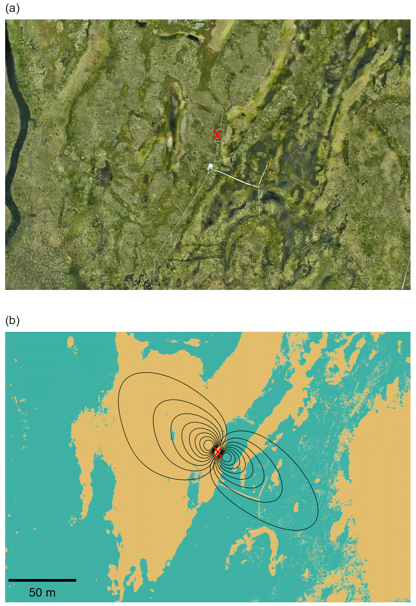
Figure 1 (a) Red–green–blue (RGB) orthomosaic of the Stordalen peatland from an unoccupied aerial vehicle (UAV) flight on 12 June 2024 and (b) the surface map derived from the digital elevation map (DEM) and flux footprints in the northwest (NW) and southeast (SE) directions. Black lines represent flux footprint contours from 10 % to 80 %, and the location of the EC tower is marked by a red cross. The yellow colour indicates the dry surface and the turquoise colour the wet surface. UAV data were provided by the Swedish Infrastructure for Ecosystem Science (SITES) under a CC BY 4.0 license; the red cross was added by the authors.

Horizontal and vertical wind components were measured with the Gill HS-50 (Gill Instrument Ltd., England, UK) ultrasonic anemometer at a frequency of 10 Hz. The sonic anemometer's north was aligned 10° east relative to geographic north. CO mixing ratios were measured using Aerodyne quantum cascade laser spectroscopy (QCLS; Aerodyne Research Inc., Billerica, MA, USA), which also simultaneously measured nitrous oxide (N₂O) and water vapour (H₂O) mixing ratios at a frequency of 10 Hz. The horizontal separation between the ultrasonic anemometer and gas inlet was 0.19 m. The EC inlet was connected to the gas analyser by a 30 m long tube with an inner diameter of 8.13 mm and an outer diameter of 12.0 mm. The gas analyser pressure was set to 4.67 kPa and regulated by an electronic valve. The gas flow rate was approximately 16.2 L min⁻¹.

2.2.2 Flux processing

The EC data processing was performed using EddyUH software (Mammarella et al., 2016), following the recommendations given in Kohonen et al. (2020) for carbonyl sulfide flux processing. Fluxes were calculated as half-hourly averages, and linear detrending was used to separate the time series into mean and fluctuating components. The coordinate system was set using a 2D-coordinate rotation according to Kaimal and Finnigan (1994). Spikes were defined using a limit of the difference between subsequent 10 Hz data points. If the difference between two data points exceeded 5 ppb for the CO mixing ratio and 5 m s⁻¹ for the vertical wind velocity component, the data point was considered to be a spike and replaced with the previous value. The time lag was determined by maximizing the cross-covariance between the CO mixing ratio and the vertical wind velocity component. Spectral corrections were applied to account for the low- and high-frequency attenuation of the covariance. High-frequency spectral corrections were made with an experimental approach (Aubinet et al., 1999). The low-frequency losses were corrected with a theoretical transfer function according to Rannik and Vesala (1999).

The measurements included a longer gap from February to April 2024 due to a broken scroll pump before its replacement. In addition, several shorter gaps occurred due to dirty inlet filters, power cuts, or other instrumentation problems, during which the flux measurements were not running. In total, the measurement period contained 24 212 calculated half-hourly fluxes, which were subsequently quality filtered. The calculated fluxes were accepted according to the following criteria: the second wind rotation angle was less than 10° in absolute value (removing 19 data points), the number of spikes in the 30 min wind vertical velocity was less than 100 (removing 1577 data points), kurtosis of the CO mixing ratio and vertical wind component was between 1 and 8 (removing 950 data points), skewness of the CO mixing ratio and vertical wind component was between −2 and 2 (removing 14 data points), and flux stationarity was less than 0.3 (removing 8981 data points). The low turbulent conditions were filtered out using a threshold value for friction velocity less than 0.1 m s⁻¹ (removing 936 data points). In addition to these criteria, a few remaining spikes were filtered based on the standard deviation of a vertical wind velocity component larger than 2 m s⁻¹ and a CO mixing ratio larger than 9 ppb (removing 100 data points). Overall, the data coverage for the measurement period was 31.7 %. The data coverage across the different seasons is summarized in Table S1 in the Supplement.

Finally, the relative contribution of the surface source area to the measured flux was calculated using the 2D Flux Footprint Prediction (FFP) model (Kljun et al., 2015). We assumed a constant boundary layer height of 1000 m because the model is insensitive to boundary layer height at low measurement heights, and we estimated the roughness length to be 0.03 m based on the logarithmic wind profile in neutral atmospheric conditions. The other model parameters, including the wind speed, wind direction, Monin–Obukhov length, standard deviation of the lateral wind velocity component, and friction velocity, were obtained as output from the EC flux post-processing. The flux footprint was presented as 90 % of the source area and was calculated for every half-hourly flux with a spatial resolution of 0.5×0.5 m.

2.3 Ancillary measurements

Ancillary data used in this study were obtained from Integrated Carbon Observation System (ICOS) measurements (Lundin et al., 2023). These data include relative humidity (RH), air pressure, air temperature (T_a), photosynthetically active radiation (PAR), water table depth (WTD), soil temperature (T_s), and SWC at 10 cm depth. T_s and WTD represent the average of four measurement plots, while SWC is based on the average of two measurement plots. A detailed description of the ICOS instrumentation at the Stordalen peatland site (SE-Sto), along with access to the ancillary dataset, is available through the ICOS Carbon Portal (https://data.icos-cp.eu/portal/, last access: 10 July 2025).

2.4 Surface map

The surface cover map was created using drone imagery and a digital elevation model (DEM) (Abisko Scientific Research Station, 2025a, b). Elevated palsas were distinguished from wetter vegetation using a DEM threshold value of 383.0 m. Pixels with a DEM value higher than the threshold were classified as dry palsas, while pixels with a DEM value lower than the threshold were classified as wet hollows. The surface cover map was saved with a resolution of 0.5×0.5 m and was used together with the footprint analysis to calculate the contribution of dry and wet surfaces to the measured half-hourly fluxes.

2.5 Definition of seasons

We defined the seasons based on the following calendar months: winter as December–February, spring as March–May, summer as June–August, and autumn as September–November. The beginning and end of the frozen period were determined according to Łakomiec et al. (2021), defined as days when the daily average peat temperature at 10 cm depth remained below/above 0 °C for 3 consecutive days. The frozen periods during the measurement period were from 21 November 2022 to 11 May 2023 and 1 November 2023 to 12 May 2024.

2.6 Statistical analysis

2.6.1 Flux driver analysis

The flux drivers were analysed using correlation analysis and a random forest (RF) model (sklearn.ensemble.RandomForestRegressor), both performed on half-hourly values. The correlation between CO flux and meteorological and environmental variables was quantified using Spearman’s rank correlation coefficients (scipy.stats.spearmanr). To assess the importance of variables in linear regression, the Akaike information criterion (AIC) was used. The AIC is a metric used to compare the fit of different regression models, designed to identify the model that best balances goodness of fit and model complexity (i.e., the number of model parameters) (Akaike, 1973). The preferred model is the one with the lowest AIC value. In our case, this criterion was used to assess whether the added complexity of including temperature as a driver of CO flux is justified in addition to PAR.

To further investigate the drivers and detect potential nonmonotonic relationships not captured by simple linear analysis and Spearman's correlations, we applied SHapley Additive exPlanation (SHAP) values derived from an RF model. This approach allows for the identification of complex, nonlinear interactions that may not be captured by traditional linear methods or by Spearman's correlation. SHAP values were calculated using the SHAP library (https://shap.readthedocs.io/, last access: 10 September 2025). The SHAP values provide a method to understand the factors driving the model's predictions by quantifying the marginal contribution of each feature to the output.

For the RF model, the data were split into a training (80 %) and a validation (20 %) set using a random split (random_split function). The hyperparameters – maximum depth (10, 12, 15, 20), number of estimators (50, 100, 150, 200), and minimum samples per leaf (2, 3, 4) – were optimized using a grid search function (sklearn.model_selection.GridSearchCV). The optimal model was selected by minimizing the mean squared error (MSE). After cross-validation, the optimal model was refit using all available data, and SHAP values were calculated. The statistical analysis in this section and the following sections was performed with Python 3.12.

2.6.2 Parametrization of carbon monoxide fluxes

Two statistical models were developed to simulate the half-hourly CO fluxes and to assess the flux contributions from wet and dry surfaces. The first model was a simple linear model assuming a homogeneous surface structure and was defined as

$$\begin{array}{}\text{(1)}& F_{\mathrm{co}}=\mathit{\alpha }\cdot \mathrm{PAR}+\mathit{\beta }\mathrm{1}\cdot T_{\mathrm{a}}+\mathit{\beta }\mathrm{2}\cdot T_{\mathrm{a}}^{\mathrm{2}}+\mathit{\gamma }\cdot \mathrm{PAR}\cdot T_{\mathrm{a}}+\mathit{\delta }.\end{array}$$

The second model was a surface-type-specific model for heterogeneous surfaces and was defined as

$$\begin{array}{}\text{(2)}& F_{\mathrm{co}}=F_{\mathrm{co},\mathrm{dry}}+F_{\mathrm{co},\mathrm{wet}},\end{array}$$

where F_co,dry and F_co,wet represent the contributions from dry and wet surface types, respectively. These components are defined as follows:

$$\begin{array}{}\text{(3)}& {\displaystyle }\begin{array}{rl}{F}_{\mathrm{co},\mathrm{dry}}& =f_{\mathrm{dry}}\cdot ({\mathit{\alpha }}_{\mathrm{dry}}\cdot \mathrm{PAR}+\mathit{\beta }{\mathrm{1}}_{\mathrm{dry}}\cdot T_{\mathrm{a}}+\mathit{\beta }{\mathrm{2}}_{\mathrm{dry}}\cdot T_{\mathrm{a}}^{\mathrm{2}}\\ & +{\mathit{\gamma }}_{\mathrm{dry}}\cdot \mathrm{PAR}\cdot T_{\mathrm{a}}+{\mathit{\delta }}_{\mathrm{dry}}),\end{array}\text{(4)}& {\displaystyle }\begin{array}{rl}{F}_{\mathrm{co},\mathrm{wet}}& =f_{\mathrm{wet}}\cdot ({\mathit{\alpha }}_{\mathrm{wet}}\cdot \mathrm{PAR}+\mathit{\beta }{\mathrm{1}}_{\mathrm{wet}}\cdot T_{\mathrm{a}}+\mathit{\beta }{\mathrm{2}}_{\mathrm{wet}}\cdot T_{\mathrm{a}}^{\mathrm{2}}\\ & +{\mathit{\gamma }}_{\mathrm{wet}}\cdot \mathrm{PAR}\cdot T_{\mathrm{a}}+{\mathit{\delta }}_{\mathrm{wet}}),\end{array}\end{array}$$

where f_dry and f_wet represent the footprint-weighted fraction of dry and wet areas, respectively, which were estimated from the surface map (Fig. 1); α represents the sensitivity of CO fluxes to PAR; β1 and β2 capture the linear and quadratic effects of T_a, respectively; γ represents the interaction between PAR and T_a; and δ is the intercept term.

The model parameters, α, β1, β2, γ, and δ, were estimated using a Bayesian inference approach. Prior selection followed the methodology proposed by Buzacott et al. (2024) with two model runs. We used the first model run to estimate the probable parameters for each land use separately using the homogeneous surface type model (Eq. 1) and the second model run to estimate the probable parameters for mixed contributions from both surface types using the heterogeneous surface type model (Eq. 2). For the first model run, all priors were assumed to follow uniform distributions (Table S3). Data were divided into wet and dry classes based on the threshold of 70 % of fluxes originating from wet or dry surfaces. In addition, the model parameters were estimated by assuming homogeneous surface structure, using all data for parameter estimation. The resulting posterior distributions were observed to follow approximately normal distributions (Supplement Fig. S8). For the second run, all available data with mixed surface contributions were used. The prior distributions were defined based on the posterior information obtained from the first model run. All prior distributions were defined as normal distributions, based on the 95 % confidence interval of the posteriors from the first model run, as suggested by Buzacott et al. (2024). The decision to use the 95 % confidence interval was made to ensure sufficient flexibility for the parameters under the mixed contribution. The priors for the second model run are presented in Table S3, and the posterior distributions from the second run are shown in Fig. S9.

The model parameters were optimized through numerical sampling using the Markov chain Monte Carlo (MCMC) method. The MCMC sampling was performed using the pm.sample function from Python’s PyMC library with 4 chains and 2000 samples in each chain, with a tuning period of 2000, totalling 8000 samples. The output product from the MCMC sampling consisted of posterior probability distributions for each optimized model parameter. The model performance for both models was evaluated by comparing the predicted fluxes to the observed fluxes, using the root mean square error (RMSE) and the coefficient of determination (R²) as performance metrics.

The models were initially fitted using data from March to November, excluding winter months. To investigate potential seasonal variability in the model parameters, separate analyses were subsequently conducted for each season (spring, summer, and autumn). An initial model using only PAR was tested, but T_a was added because it improved model performance (Table S2). The posterior parameter estimates from the final model were then used to simulate CO fluxes from both wet and dry surface types. Annual estimates were derived by applying these posterior parameters to observed PAR and T_a data from March to November, under the assumption that wintertime fluxes were negligible and therefore set to zero.

3 Results

3.1 Environmental conditions and flux footprint

The mean annual temperature for the first measurement year (from August 2022 to August 2023) was 1.1 °C, while the mean annual temperature for the second measurement year (from August 2023 to August 2024) was −0.1 °C. The first year was warmer than the long-term average annual temperature (1991–2020), while the second year was colder than the long-term average (SMHI, 2024). The air temperature during the measurement period ranged from −38.8 to 27.3 °C; the minimum value was observed on 4 January 2024 and the maximum value on 22 July 2024. The soil temperature at a depth of 10 cm ranged from −12.2 to 11.3 °C, with the minimum recorded on 4 January 2024 and the maximum value observed on 22 July 2024. The total accumulated precipitation was 325 mm in the first measurement year and 298 mm in the second year. In both years, annual precipitation was lower than the long-term average (1991–2020) for this region (SMHI, 2024). The daily mean PAR varied from 0.2 to 688.4 µmol m⁻² s⁻¹, with the minimum value observed on 31 December 2022 and the maximum value on 1 July 2024.

The main wind directions during the study period were from the southeast (SE) and the northwest (NW), with 45 % of the measured fluxes coming from the wind sector between 40 and 180° (SE) and 54 % from the wind sector between 200 and 350° (NW). The distribution of wind directions was consistent across different seasons and stability classes (Fig. S1), although slight day–night differences were observed during the non-frozen period, with SE winds more common at night and NW winds more frequent during the day (Fig. S2). The footprint-weighted average showed that fluxes from the NW wind direction were predominantly associated with the drier palsas, with 93 % of the fluxes originating from the palsas and 7 % of the fluxes originating from the wetter surface (Fig. 1). In contrast, fluxes from the SE direction were characterized by 23 % originating from the drier palsas and 77 % from the wetter surface.

3.2 Ecosystem-scale fluxes

3.2.1 Flux time series

The ecosystem-scale half-hourly CO fluxes ranged from −0.29 to 0.39 nmol m⁻² s⁻¹ (25th and 75th percentiles), showing both net uptake and emission. The fluxes had strong seasonal variability, with the site acting as a net CO source in spring and summer (average median fluxes of 0.19 and 0.29 nmol m⁻² s⁻¹, respectively) and a net sink in autumn (−0.34 nmol m⁻² s⁻¹) (Fig. 2). The wintertime flux was minor (−0.06 nmol m⁻² s⁻¹) compared to the fluxes of other seasons. This seasonal pattern was consistent across both years.

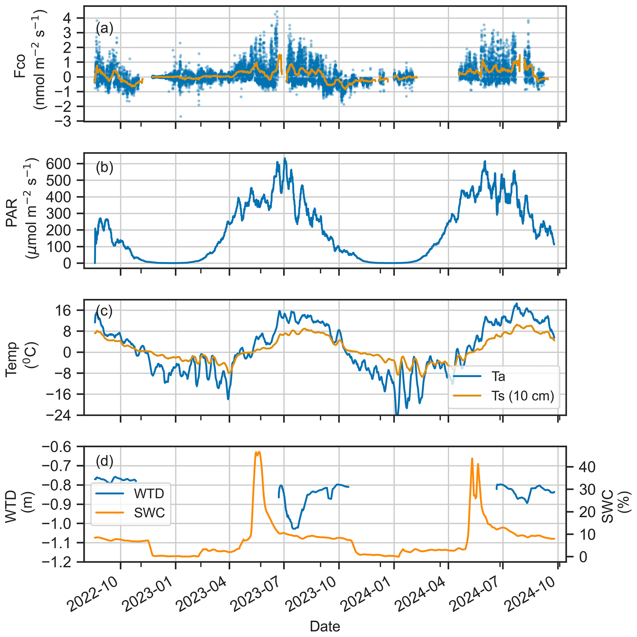
Figure 2 Time series of (a) CO flux, (b) photosynthetically active radiation (PAR), (c) air temperature (T_a) and soil temperature at 10 cm depth (T_s), and (d) water table depth (WTD) and soil water content (SWC) at 10 cm depth. The solid line represents the 7 d rolling average (a–d), and the dots indicate half-hourly flux (a).

The CO flux showed a systematic diurnal cycle during the vegetative period, with daytime emissions and nighttime uptake. Emissions peaked at noon, reaching 1.26 nmol m⁻² s⁻¹ in summer and 0.80 nmol m⁻² s⁻¹ in spring, while nighttime uptake was the strongest in autumn (−0.48 nmol m⁻² s⁻¹) (Fig. 3). In contrast, winter fluxes lacked a clear diurnal cycle. The diurnal pattern reflected seasonal differences, with net positive daily fluxes (emissions) in spring and summer and net negative fluxes (uptake) in autumn.

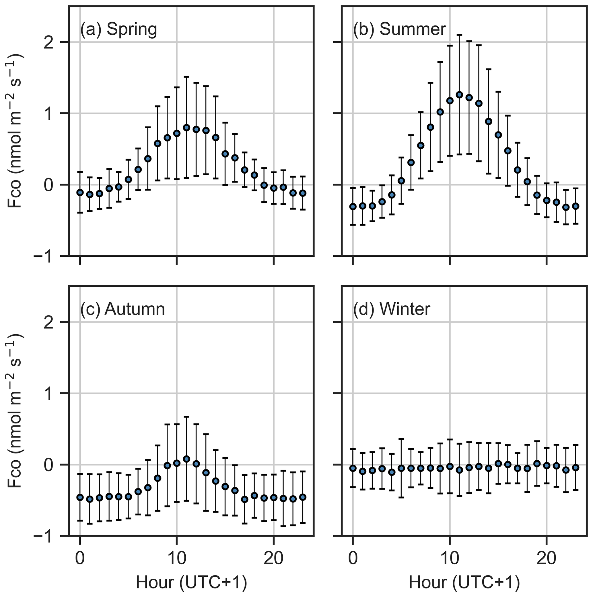
Figure 3 Diurnal cycle of CO flux (mean and standard deviation) in (a) spring, (b) summer, (c) autumn, and (d) winter.

3.2.2 Flux drivers

Seasonal and diurnal variations in CO fluxes were primarily driven by the seasonal and diurnal cycles of environmental conditions during the unfrozen period (Fig. 2). We found no significant correlation between wintertime fluxes and any environmental conditions (Fig. S3), and wintertime fluxes were thus excluded from further analysis, with a focus on other seasons. Spearman rank correlations showed that PAR and temperature were the key factors explaining flux dynamics (Fig. 4). We found a positive correlation between half-hourly CO flux and both PAR (0.75) and T_a (0.36), indicating that fluxes increase with higher radiation and warmer temperatures.

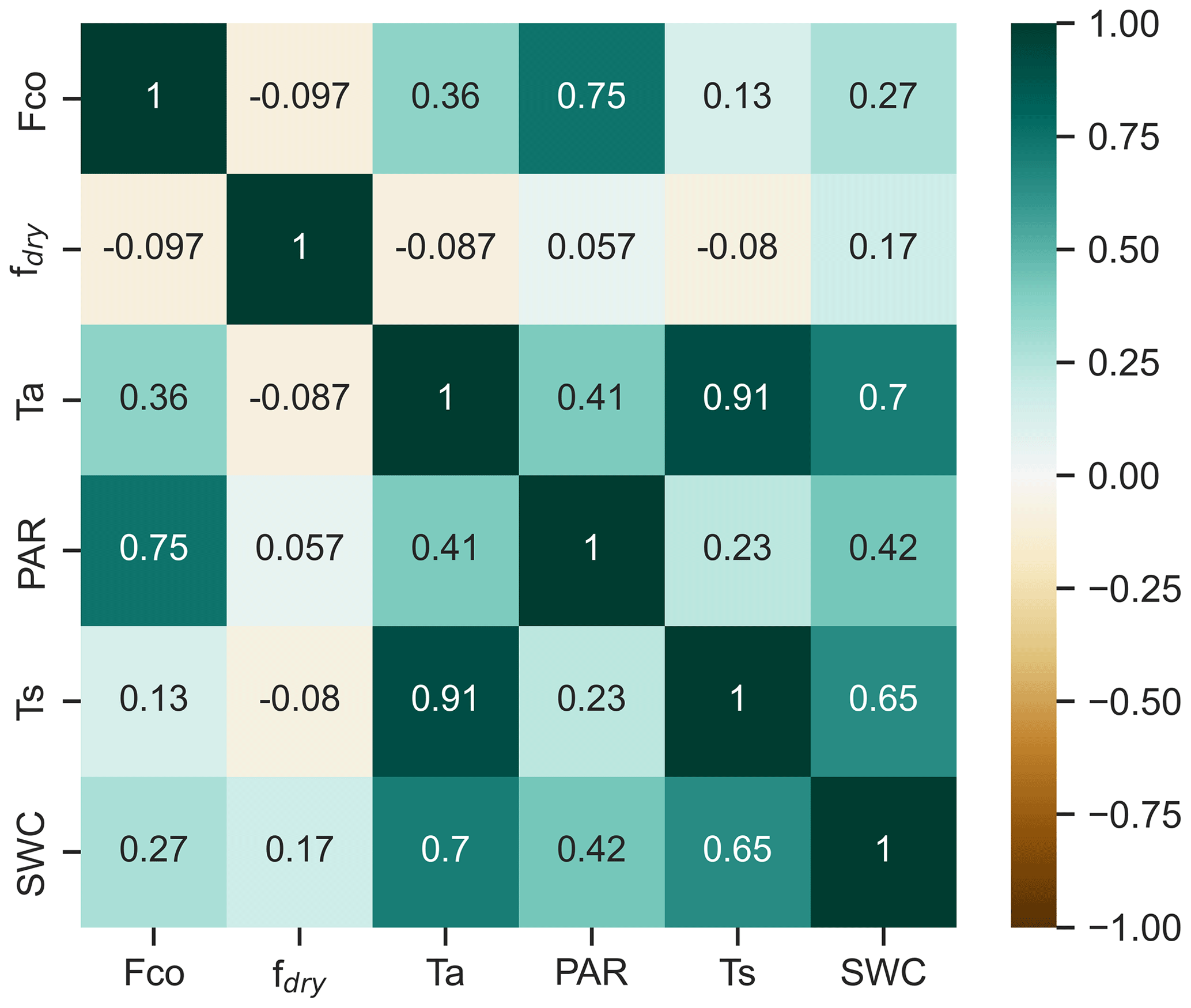
Figure 4 The correlation matrix of Spearman's rank correlation coefficients for CO flux (F_co) and flux drivers: soil temperature at a depth of 10 cm (T_s), photosynthetically active radiation (PAR), air temperature (T_a), and fraction of dry surface area (f_dry), calculated for half-hourly values during March–November.

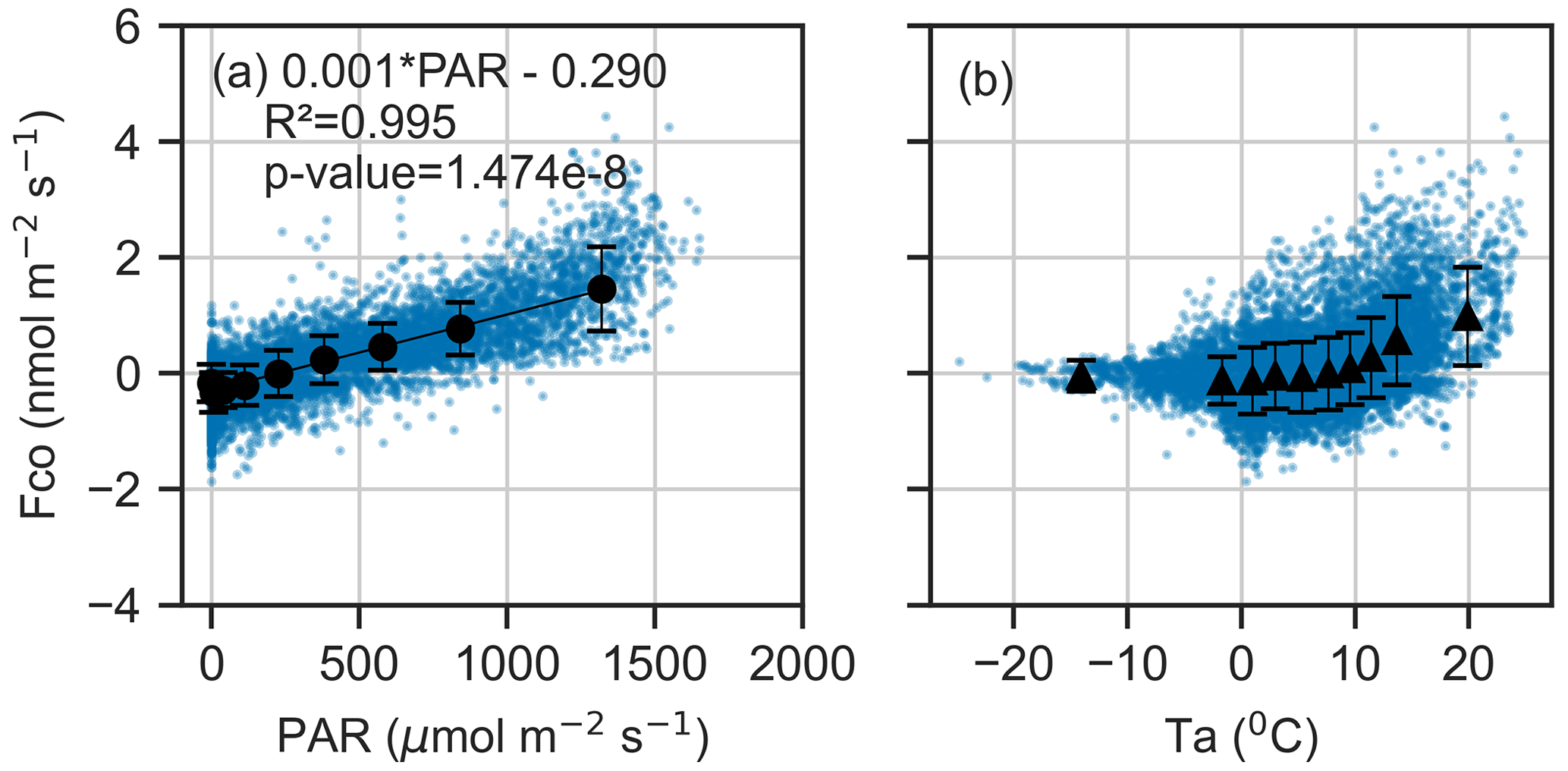
Figure 5 Binned mean and standard deviation between CO flux and (a) photosynthetically active radiation (PAR) and (b) air temperature (T_a) during March–November. The data are divided into 10 equally sized bins, and blue dots represent the 30 min fluxes. A linear regression line is fitted to PAR.

The analysis revealed a strong linear relationship between CO flux and PAR (R²=0.995, $p=\mathrm{1.47}\times {\mathrm{10}}^{-\mathrm{8}}$), with a regression slope of 0.0013 nmol m⁻² s⁻¹ and intercept of −0.30 nmol m⁻² s⁻¹ (Fig. 5). The CO flux approached zero at approximately 250 µmol m⁻² s⁻¹ PAR, a threshold that aligned with seasonal shifts in net CO flux observed in the time series (Fig. 2). A nonlinear relationship was found between the CO flux and T_a (Figs. 5, S4). Including T_a in the linear model reduced the AIC from 10 120 (PAR only) to 9787, suggesting that T_a is also a significant explanatory variable for CO exchange.

According to Spearman’s rank correlations, the correlation between CO flux and T_s (0.13) was smaller than between the CO flux and T_a (0.36) (Fig. 4). However, soil temperature played an important role, especially in spring and autumn flux dynamics, when the soil was frozen or unfrozen. The systematic soil consumption observed in the nighttime flux began in spring after the soil melted and ceased in autumn once the soil froze (Fig. 2). In the nighttime data, a higher negative correlation was found with T_s (−0.39) than with T_a (−0.29) (Fig. S5). The correlation analysis including the daytime and nighttime fluxes did not reveal any clear relationship between the CO flux and f_dry (Fig. 4). However, in the nighttime fluxes, a negative correlation between CO flux and f_dry (−0.30) was observed (Fig. S5).

The results from the SHAP values were consistent with the results of the Spearman correlations, with the highest positive fluxes associated with high PAR (Fig. 6). T_s and T_a were found to be the second- and third-most important drivers, with higher positive fluxes (emission) associated with low soil temperature and high air temperature. In the nighttime data, T_s was the most important driver, with the higher negative fluxes (uptake) associated with high soil temperature (Fig. S6), consistent with Fig. 6. Additionally, SHAP values from all data and nighttime data indicated that higher f_dry led to decreased fluxes, meaning that higher fluxes were observed in the wetter conditions (Figs. 6, S6). Figure S7 presents partial dependence plots of SHAP values for each feature.

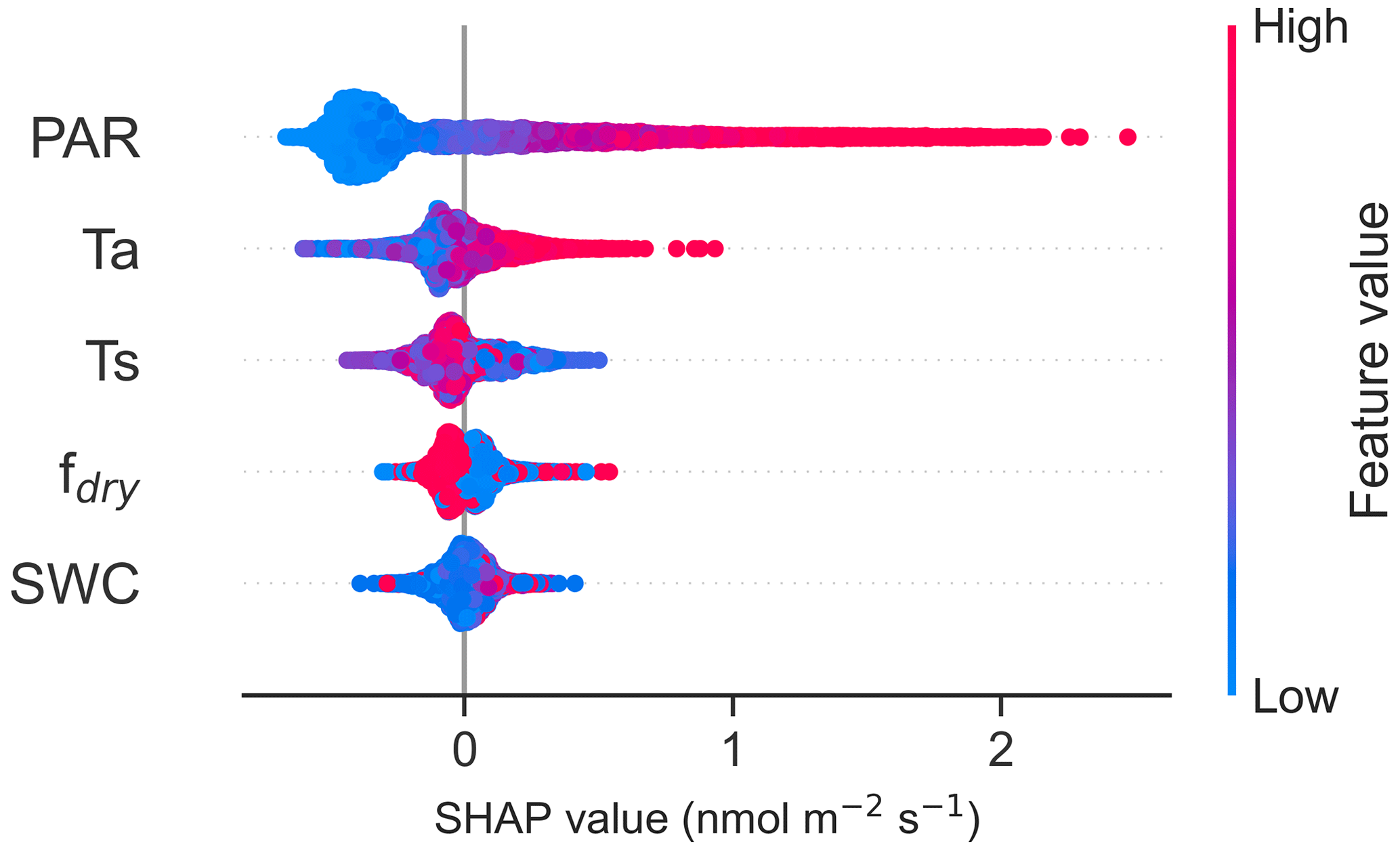
Figure 6 The SHapley Additive exPlanation (SHAP) values of the random forest (RF) model for CO flux drivers photosynthetically active radiation (PAR), air temperature (T_a), soil temperature at a depth of 10 cm (T_s), soil water content at a depth of 10 cm (SWC), and fraction of dry surface area (f_dry). The SHAP values indicate the impact each feature has on the model output, with a negative value indicating a reduced flux and a positive value an increased flux. The blue colour represents low feature values and the red colour high feature values. The zero line is the baseline (the average prediction). The SHAP values were calculated using the data collected from March to November.

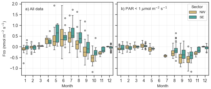
Figure 7 The boxplot of NW (yellow) and SE (turquoise) CO fluxes in different months (a) for all PAR levels and (b) in dark conditions for PAR < 1 µmol m⁻² s⁻¹. The box represents the interquartile range (IQR), with the lower limit at the 25th percentile and the upper limit at the 75th percentile, while the whiskers indicate the minimum and maximum values. Black dots represent outliers, defined as 1.5 × IQR.

We analysed the CO fluxes from the NW and SE footprints and found that fluxes from the NW footprint were consistently lower than those from the SE footprint throughout the study period (Fig. 7). On average, the net flux from the NW footprint was 0.04 nmol m⁻² s⁻¹, whereas the net flux from the SE footprint was 0.15 nmol m⁻² s⁻¹. The nighttime flux from the NW footprint was on average 2.1 times larger than in the SE footprint (−0.24 nmol m⁻² s⁻¹ in NW vs. −0.13 nmol m⁻² s⁻¹ in SE). For example, in July, the mean nighttime flux from the NW footprint was −0.28 nmol m⁻² s⁻¹ compared to −0.13 nmol m⁻² s⁻¹ from the SE footprint. This pattern was observed across all months, with the exception of April, when the SE footprint exhibited slightly lower fluxes (0.06 nmol m⁻² s⁻¹ in NW vs. 0.03 nmol m⁻² s⁻¹ in SE). The consistently lower nighttime fluxes from the NW footprint suggest greater CO uptake by the soil in this area compared to the SE footprint.

3.3 Estimate of fluxes from dry and wet surfaces using Bayesian inference

3.3.1 Parameter distributions and model performance

Seasonal and surface-type-dependent variability was evident in the estimated model parameters, highlighting the influence of both environmental conditions and surface heterogeneity on CO exchange dynamics (Fig. S9). The seasonal differences were less pronounced when T_a was included as an explanatory variable compared to the model using only PAR, suggesting that part of the observed seasonality was explained by temperature. The intercept parameter (δ) exhibited clear seasonal patterns: values were higher compared to other seasons in spring (${\mathit{\delta }}_{\mathrm{dry}}=-\mathrm{0.124}$ and ${\mathit{\delta }}_{\mathrm{wet}}=-\mathrm{0.127}$ nmol m⁻² s⁻¹), indicating reduced CO uptake when the soil remained frozen. In contrast, lower intercepts were observed in summer (${\mathit{\delta }}_{\mathrm{dry}}=-\mathrm{0.563}$ and ${\mathit{\delta }}_{\mathrm{wet}}=-\mathrm{0.206}$ nmol m⁻² s⁻¹) and autumn (${\mathit{\delta }}_{\mathrm{dry}}=-\mathrm{0.645}$ and ${\mathit{\delta }}_{\mathrm{wet}}=-\mathrm{0.233}$ nmol m⁻² s⁻¹), reflecting enhanced uptake during warmer conditions. The intercept was lower on dry surfaces than on wet surfaces during summer and autumn, whereas no such difference was observed in spring. Seasonal and surface-dependent variations were also apparent in other model parameters; however, the interpretation is complicated by the collinearity between PAR and T_a, which may confound individual parameter estimates and limit the ability to isolate their respective effects.

Model performance was calculated using the posterior parameter sets from the second run and is presented in Table S4. The RMSE between different models ranged from 0.34 nmol m⁻² s⁻¹ to 0.39 nmol m⁻² s⁻¹, and R² values ranged from 0.28 to 0.79. Overall, the model performance was the best in summer and the poorest in autumn. The mean of the predicted values follows the 1:1 line, with no obvious bias towards high or low values (Fig. S10). The model performance was slightly better in the heterogeneous surface models compared to the homogeneous surface models, with an average RMSE improvement of approximately 0.015 nmol m⁻² s⁻¹ and R² increases of 0.036.

3.3.2 Annual cumulative flux

We estimated the annual cumulative fluxes applying the posterior parameters from our seasonal model to the PAR and T_a data from March to November (Fig. S9). The difference in annual fluxes between the seasonally parameterized and non-seasonally parameterized models was small (Fig. S11). However, as we observed seasonal variation in model parameters, we chose to use the seasonal model for calculating annual fluxes to better represent temporal dynamics. The annual cumulative flux for dry surfaces was −32.6 mg CO m⁻² yr⁻¹ in 2022–2023 and −17.1 mg CO mg CO m⁻² yr⁻¹ in 2023–2024, while for wet surfaces, it was 84.0 mg CO m⁻² yr⁻¹ in 2022–2023 and 83.4 mg CO m⁻² yr⁻¹ in 2023–2024. There was a significant difference between wet and dry surfaces, with dry surfaces acting as CO sinks and wet surfaces as CO sources. Interannual variability in annual cumulative fluxes was minor. The cumulative annual flux in the homogeneous model was 10.0 mg CO m⁻² yr⁻¹ in 2022–2023 and 22.5 mg CO m⁻² yr⁻¹ in 2023–2024. The confidence intervals and standard deviations of annual estimates are presented in Table S5.

4 Discussion

4.1 Flux magnitude and temporal variations

Our results show that CO flux dynamics are influenced by environmental conditions, particularly radiation and temperature, and vary according to the surface cover type. We found that the wet surfaces of the peatland emit CO, while the drier areas of the peatland act as CO sinks. This study provides new insights into the magnitude and drivers of biogenic CO fluxes in Arctic peatlands, contributing to a better understanding of the role of terrestrial ecosystems in the CO budget.

The CO fluxes reported in this study are similar in magnitude to the fluxes reported in previous EC flux studies in a boreal cropland and two temperate grasslands, with mean fluxes ranging from −1 to 2 nmol m⁻² s⁻¹ (Pihlatie et al., 2016; Cowan et al., 2018; Murphy et al., 2023). The modelled annual fluxes in this study ranged from −33 to −84 mg CO m⁻² yr⁻¹. When compared with annual fluxes reported in other EC studies, particularly from temperate regions where values range from 360 to 880 mg CO m⁻² yr⁻¹ (Cowan et al., 2018; Murphy et al., 2023), our results indicate a lower contribution of biogenic CO emissions from Arctic peatlands relative to temperate grasslands.

Consistent with earlier studies, our results show clear seasonal variations in CO fluxes (Pihlatie et al., 2016; Cowan et al., 2018). The site acted as a net source of biogenic CO during the spring and summer and a net sink during the autumn. The highest net emissions were observed in summer, although the difference between summer and spring was smaller than would be expected if fluxes were determined solely by radiation from living plants. Spring emissions began even before snowmelt and the onset of the growing season, suggesting that CO degradation from senescent plants and litter from the previous year may contribute to the emissions. This is also supported by other studies reporting that senescent plants and litter emit higher amounts of CO than living plants (Tarr et al., 1995; Derendorp et al., 2011; Lee et al., 2012). Early spring CO emissions were reported by Pihlatie et al. (2016) from reed canary grass, where high emissions were observed after snowmelt before the start of crop growth. Another factor probably contributing to the relatively high net emissions in the spring was frozen soil, which results in significantly lower nighttime CO consumption compared to the summer and autumn periods.

The largest net CO consumption was observed during late summer and early autumn in the nighttime data. Nighttime was defined as periods when PAR was less than 1 µmol m⁻² s⁻¹. In high latitudes, dark conditions during mid-summer are limited, and therefore we have only limited nighttime data available for the summer months. The summer diurnal plot (Fig. 3) includes the effects of radiation on fluxes during nighttime hours (19:00 to 04:00 LT), when net uptake was observed, making it difficult to fully understand the development of soil uptake throughout the growing season. However, we observed that the highest net uptake occurred in late summer and autumn. We speculate that microbial communities responsible for CO consumption require time to develop (King and Weber, 2007; Cordero et al., 2019), which could explain the higher consumption in late summer and autumn rather than in early or mid-summer. In autumn, when CO production ceases due to PAR limitation, consumption became more visible and was also observed in daytime fluxes. In August, both soil and air temperature were higher than in September and October, suggesting that thermal production, in the absence of radiation, may influence the net flux and reduce CO consumption.

The importance of soil temperature as a driver of CO fluxes increased in autumn, when the site was mainly a net sink of CO. The transition from a net source to a net sink of CO occurred when the PAR level dropped below 250 µmol m⁻² s⁻¹. This shift from a net source to a net sink in autumn is a result of a decreased photoproduction of CO due to limited daytime radiation in high latitudes and may also indicate increased CO consumption in the soil. A similar shift has also been observed in a boreal cropland (Pihlatie et al., 2016) but not in temperate ecosystems (Cowan et al., 2018; Murphy et al., 2023). The soil consumption in autumn continued until the soil froze.

The contribution of wintertime fluxes to the total CO flux was relatively small compared to fluxes observed in other seasons, likely due to both limited production and consumption. The lack of correlation between wintertime fluxes and environmental variables suggests minimal CO activity during winter or at least no significant process that would result in a net flux different from zero. The limited daylight and snow cover may prevent CO emissions, while CO consumption likely ceased due to frozen soil. Due to the small flux during the winter, this study focused primarily on spring, the growing season, and autumn fluxes.

4.2 Processes and flux drivers

We observed a systematic diurnal cycle, with daytime emissions peaking at noon and nighttime uptake, a pattern consistent with other studies (Pihlatie et al., 2016; Cowan et al., 2018). Daytime emissions followed the pattern of PAR, suggesting that CO production is driven by radiation, likely due to photodegradation of organic matter, litter, or living plants (Tarr et al., 1995; Derendorp et al., 2011; King et al., 2012; Bruhn et al., 2013; Muller et al., 2025). Our flux driver analysis indicated that PAR is the primary factor driving ecosystem-scale CO fluxes. The linear relationship between PAR and CO, also reported in Bruhn et al. (2013), suggests an underlying abiotic process, with no obvious limiting biotic factors controlling the emissions. However, thermal production (Lee et al., 2012; van Asperen et al., 2015) and biotic production of living plants (Wang and Liao, 2016) have also been reported as potential sources of CO at the ecosystem scale. For example, a recent study found that heat-controlled biogenic CO production from plants is linked to biotic processes rather than photoproduction (Muller et al., 2025). Unfortunately, using the EC technique, we cannot determine the exact source process of these emissions.

Our analysis indicates that air temperature is an important factor influencing CO exchange. Both AIC and SHAP values indicate that air temperature is a statistically significant driver, together with PAR, with higher emission observed at warmer temperatures. This was also supported by our residual analysis, which revealed a nonlinear relationship in the flux residuals derived from the linear model of PAR (Fig. S4). Due to the correlation between temperature and radiation, it is challenging to fully disentangle their independent effects on CO fluxes. We propose that photodegradation and thermal degradation may occur simultaneously. However, as the net nighttime CO fluxes were mostly negative, if thermal degradation does occur, it is likely much smaller than the observed nighttime CO consumption. The measured nighttime CO consumption is hence a net sum of microbial CO consumption and abiotic CO production via thermal degradation, both of which are likely driven by temperature. However, we cannot exclude the possibility of heat-controlled biotic sources contributing to CO fluxes (Muller et al., 2025).

According to our driver analysis, we were not able to identify relationships between environmental drivers and CO uptake as clearly as we did for CO emissions. We found that soil temperature was an important driver, and CO uptake was observed only during the unfrozen periods. However, we did not find any clear relationship between soil temperature and CO flux during the unfrozen period. Several factors may explain this: during the daytime, net fluxes were primarily driven by radiation, and at nighttime, when CO uptake was observed, the data were limited due to low turbulent conditions and the lack of dark conditions in summer. As mentioned earlier, thermal production, which is the one potential source of CO, and soil consumption are both likely driven by temperature, which may lead to similar responses for each process, thereby minimizing the changes observed in net flux (King, 2000).

In addition to temperature, SWC has been proposed as a potential driver of CO uptake. Low SWC can limit microbial processes, while high SWC may prevent gas diffusion in the soil (Moxley and Smith, 1998). However, we could not identify a clear relationship between CO flux and SWC, but we observed systematically lower fluxes from the drier footprint compared to the wetter footprint. This was seen in both daytime and nighttime data, as well as in SHAP values. The higher consumption observed in drier conditions suggests that CO uptake is larger under oxic conditions than under anoxic conditions. This is consistent with other studies, which have found that most CO consumption occurs under oxic conditions (Funk et al., 1994; Rich and King, 1999). This is expected, as CO is reactive and can be oxidized to CO₂ (Bartholomew and Alexander, 1979; King and Weber, 2007). It is also possible that in wet conditions, CO diffusion was prevented in the soil, as proposed in Moxley and Smith (1998).

4.3 Flux modelling

We used the regression model to estimate CO fluxes from the dry and wet surfaces and to calculate the annual fluxes from these two surfaces. The modelling approach has its own limitations in terms of data coverage and the modelling approach used. Our data coverage for the full measurement period was 31.7 %, which is relatively low but within the expected range for EC measurements for gases with a low signal-to-noise ratio. In the data filtering, we followed standard quality control procedures (Mauder and Foken, 2006), with the most common reason for data exclusion being failure to meet the stationarity criterion. The limited data coverage causes uncertainty in the annual fluxes, especially during nighttime and spring and autumn seasons when fewer data points are available.

We observed seasonal variability in the model parameters (Fig. S9), and thus to reduce the potential seasonal bias caused by uneven data distribution, we applied seasonal parameterization in the model. However, the comparison between the seasonal and non-seasonal models showed no significant difference in annual flux estimates (Fig. S11), suggesting that the seasonal biases do not lead to major errors in the overall annual budgets.

It is important to note that the annual fluxes reported in this study are based on modelled estimates. The model performed well for the existing dataset and was used as a tool to estimate fluxes for both wet and dry surfaces. However, we did not test the model’s predictive power on unseen data. In particular, the second-degree polynomial function used to represent the temperature response may not generalize well to other years or conditions. Furthermore, the use of this function during winter may lead to overestimation of fluxes at low temperatures, as the polynomial structure predicts emissions in cold conditions.

The heterogeneous surface structure models are found to perform better than homogeneous models in heterogeneous EC footprints (Ludwig et al., 2024; Tikkasalo et al., 2025). In our analysis, the heterogeneous model performed better than the homogeneous model, reducing RMSE by 2.0 %–7.5 %. The parameter distributions of the homogeneous model typically settled between the wet and dry parameter distributions, most often closer to the dry distributions. The reason that the homogenous parameters were closer to the dry surface type is likely related to wind directions, which show a slight bias toward the NW (Fig. S1). If the wind direction distributions were more strongly biased toward a single wind direction, a larger difference in model performance between the heterogeneous and homogeneous models could be expected. We also found that the SE footprint contained a higher proportion of nighttime data compared to the NW footprint, which may introduce a potential bias in the model, as fluxes in the SE region could be underestimated due to the lower turbulent conditions (Fig. S2). However, we consider the impact on our modelling approach and results to be minimal.

4.4 Future research

The Stordalen peatland has slowly transitioned from dry, permafrost-dominated palsa areas to wetter, sedge-dominated fens due to global warming (Varner et al., 2022). The land cover changes have been observed on decadal timescales (Varner et al., 2022). This is also important in terms of CO exchange because in the future, we can expect increased surface wetness (more sedge- and open-water-dominated vegetation), which may also lead to higher CO emissions. To better understand the annual variability and future changes in CO fluxes, longer-term measurements are needed.

In our 2-year study period, we did not expect significant changes in the wet and dry surface classes at either seasonal or annual scale. This assumption is important, as to accurately characterize heterogenous EC fluxes, we need an accurate surface cover classification. The seasonality of surface wetness in the Stordalen peatland was studied by Łakomiec et al. (2021), and they did not observe any significant seasonal changes in wet and dry classes. However, in the model, we assumed that the flux from each wet and dry pixel had uniform responses within each area. In practice, this assumption may not be valid, as the vegetation within each surface class may not be completely homogeneous. In the wet class in particular, the surface structure is a mixture of open-water areas, sedges, and mosses, which likely contribute differently to the flux. We can expect seasonal and annual variations in open-water areas and sedge cover on the peatland, even though it does not directly affect our wet and dry classification. To better understand the contribution of different surface structures within the wet and dry classes, other methods, such as chamber measurements, are needed.

Although the annual CO flux from the Stordalen peatland is relatively low, our findings suggest that current process-based models may inaccurately represent wetlands as CO sinks rather than sources (Guenther et al., 2012; Liu et al., 2018). When compared to the process-based CO model by Liu et al. (2018), our CO fluxes show a clear divergence. In that model, non-forested boreal wetlands are classified as a small CO sink, with an average annual flux of −217 mg CO m⁻² yr⁻¹. In contrast, our results indicate that these ecosystems may act as net CO sources, emphasizing the need for further research to better understand the environmental drivers and variability of CO fluxes at the ecosystem scale in high-latitude wetlands.

5 Conclusions

To interpret the role of wetlands in the global CO budget, we studied ecosystem-scale CO fluxes in Arctic peatlands. Our results revealed previously unknown biogenic sources of CO from northern peatlands to the atmosphere. The reason that these sources were unknown is partly due to the lack of long-term measurements at the ecosystem level but also an incomplete understanding of CO processes. We also report that CO flux magnitude depends on surface wetness with uptake from dry areas and emission from wet areas. This study provides a new dataset that is valuable for modelling and a new parameterization of current process-based CO models. Our study suggests that current global models may underestimate the CO source from northern wetlands.