Technical note: Comparison of simultaneously applied chamber-based gas flux measurements from arable soils using gas chromatography (static chamber) and mid-infrared laser absorption spectroscopy (dynamic chamber)

For the study of soil-atmosphere exchange of greenhouse gases, a commonly adopted method is to monitor the change of gas concentrations in closed chambers. Accurate determination of CO₂, CH₄, and N₂O concentrations is therefore essential for reliable flux estimations. This study compares two techniques to determine these gas concentrations: Gas Chromatography (GC) and mid-infrared laser absorption spectroscopy (LAS). We compared both techniques by carrying out simultaneous chamber measurements under field conditions on two separate days covering a range of fluxes. The GC method involved syringe sampling into gas-tight vials and subsequent laboratory analysis. In contrast to that, a LAS analyzer was directly connected to the chambers (tubing system) and thus enabled real-time, high-temporal resolution data. We calculated gas fluxes based on GC- and LAS-derived concentration measurements, using seven distinct flux calculation setups, including systematic variations in chamber enclosure times (30, 20 and 10 min) for LAS data. Across both measurement days, the comparison resulted in a high level of agreement for determined CO₂ fluxes with a normalized Root Mean Square Error (nRMSE): 5.79 %–16.70 %. A high level of agreement between the methods was also observed for N₂O fluxes (nRMSE: 14.63 %–24.64 %). In contrast, there was a comparatively low agreement between methods for CH₄ fluxes (nRMSE: 88.42 %–94.54 %). N₂O and CH₄ fluxes highlighted the superior precision of LAS, as it detected significant fluxes (> minimum detectable flux) that were not significant with GC. For CH₄ this explains the low agreement between methods regarding arable soils that are dominated by (low) CH₄-consumption fluxes.

1 Introduction

Various methods are available to determine greenhouse gas (GHG) fluxes at the atmosphere-soil interface. A common and versatile approach to determine GHG fluxes like carbon dioxide (CO₂), nitrous oxide (N₂O), and methane (CH₄) in field experiments is the closed chamber method, where the soil surface is temporarily covered by a chamber attached to a collar that is permanently anchored in the soil to ensure an air-tight seal when the chamber is placed on top of it (Livingston and Hutchinson, 1995). The gas flux rate is then calculated based on the measured change in gas concentration within the chamber headspace over time, using either a linear or non-linear model (Lundegardh, 1927; Hutchinson and Mosier, 1981; Yu and Yao, 2017; Maier et al., 2022). Ultimately, numerous analytical techniques are available for measuring these GHG concentrations, with decisions influenced by specific research questions and logistical feasibility. Gas concentrations required for flux calculations can be determined through real-time monitoring using online analyzers, or by collecting discrete gas samples for subsequent analysis via gas chromatography (GC), followed by peak integration to estimate gas concentrations. In both cases, flux calculation procedures demand variables according to the ideal gas law such as chamber volume, temperature and local atmospheric air pressure and the resulting flux rates are subsequently referenced to the covered soil surface (Livingston and Hutchinson, 1995).

Besides the chamber design, the choice of the gas analytical technique can be an influential factor estimating GHG fluxes in the ecosystems under investigation. For example, a comparison between cavity ring-down spectroscopy (CRDS) and GC (Christiansen et al., 2015a) showed that CRDS resulted in higher calculated CO₂ fluxes, provided comparable results for N₂O, and was significantly more sensitive for CH₄ fluxes compared to GC. The authors concluded, that both CRDS and GC were equally effective in capturing treatment effects for CO₂ and N₂O in laboratory and field settings, whereas this was not the case for CH₄. Zheng et al. (2008) pointed out, that measuring N₂O concentrations using GC with an Electron Capture Detector (ECD), the common practice using nitrogen (N₂) as a carrier gas can lead to overestimated N₂O emissions, especially in the presence of CO₂ or from weak sources (<200 µg N m⁻² h⁻¹), even if CO₂ is separated before the ECD via column separation. To address this issue, they suggest using alternative methods, for instance chemical removal of CO₂. Although the GC has commonly been used in the past, new modern online analyzers based e.g. on mid-infrared laser absorption spectroscopy (LAS) allow real-time concentration measurements within the chamber where analytical values are immediately displayed, as opposed to the GC analysis which does not allow this in most cases due to the time gap between taking samples and subsequently analyzing them; exceptions being a GC mounted in a van or container in the field to a multiplexer plus automated chamber system (e.g. Flessa et al., 2002; Yao et al., 2009). An immediate display of the measured concentration, e.g. with an LAS analyzer, provides the advantage of immediate detection of methodological set-up issues, such as leaks in chambers or tubing, enabling corrections or repetitions as necessary. Furthermore, LAS typically offer higher analytical precision, thus enabling the detection of smaller flux rates and more precise measurements within the low concentration range, which means that the minimum detectable flux (MDF) is reduced notably (Christiansen et al., 2015a; Nickerson, 2016).

Several components of the closed chamber method significantly affect MDF, including effective chamber height (ratio of volume to emitting surface), closure duration, sampling frequency during closure (i.e., periodicity), and the analytical precision of gas analysis technique as reported by Christiansen et al. (2015a) and Nickerson (2016). Substantial advancements in analytical precision and temporal resolution have led to markedly improved accuracy of GHG flux measurements, enabling shorter chamber closure times (Brümmer et al., 2017; Johannesson et al., 2024) and thereby minimizing disturbance and flux gradient alteration (Livingston and Hutchinson, 1995; Maier et al., 2022). This study aims to serve as a pilot study on the comparability of the world-wide very common GC method and fast developing LAS analyzers. A challenge of adoption of new technology is also that it changes the inherent measurement uncertainties, thus, knowledge about the impact of the gas analytical method on the gas fluxes are required (Cowan et al., 2025; Kong et al., 2025). Thus, the objective is to assess how closely the GHG flux values from both methods align and to evaluate the limitations of each method in terms of measurement accuracy. For this purpose, we conducted closed chamber measurements using simultaneously static (GC) and dynamic (LAS) approaches under field conditions and calculated the corresponding MDF.

2 Material and methods

2.1 Site description

The measurements were carried out in a long-term field experiment (LTE), initiated in 2010, which is well described in Bilibio et al. (2025). The LTE is located near Neu-Eichenberg, Hesse, Germany (223 m a.s.l., 51°22^′ N 9°54^′ E), within an organic research station operated by the University of Kassel which is further described in Leisch et al. (2025). The geological formation (Keuper) is covered by a loess layer up to a thickness of 1.8 m. The soil, characterized as a silty loam, is classified as a Luvisol (Obalum et al., 2019). It consists of 13 % clay, 84 % silt, and 3 % sand, with an organic matter content of 2 % (Schmidt et al., 2017). Over a 30-year period (1991 to 2020), the average annual temperature recorded was 9.3 °C, accompanied by an average annual precipitation of 663 mm. The climate is categorized as warm-temperate and fully humid with warm summers (Kottek et al., 2006) i.e. Cfb according to the Köppen-Geiger climate classification.

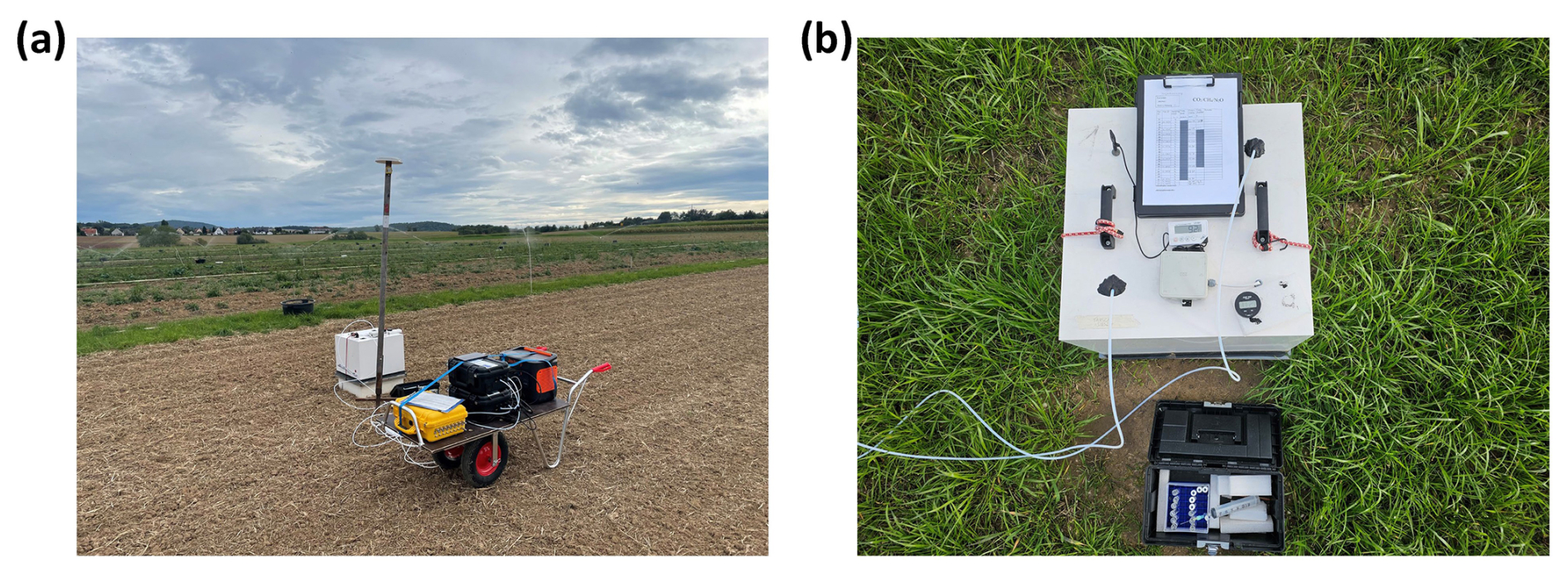
Figure 1 Field sampling after winter wheat and tillage on 21 September 2023 (a) and in a clover grass mixture on 24 March 2024 (b).

2.2 Experimental design and flux estimation

For the method comparison between GC and LAS, fluxes were determined on two dates (21 September 2023, after winter wheat harvest and tillage, and 24 March 2024, in the subsequent clover-grass mixture) in four replicated plots (Fig. 1) containing two treatments differing in organic fertilization. This resulted in 16 sets of comparative data. No fertilization was applied to the winter wheat itself. The last fertilization before the experiment was carried out at the end of the winter cover crop season 2021/22 (19 April 2022). All plots received 100 kg N ha⁻¹ as hair meal pellets, while one treatment additionally received green waste compost (5 t ha⁻¹ a⁻¹ dry matter) applied on the same day. Prior to the first flux measurement in September 2023, a series of soil tillage operations was conducted. These interventions included straw chopping and harrowing on 13 August 2023; rotary tillage to a depth of ∼4 cm on 12 September 2023; and, on 17 September 2023, loosening with a subsoiler to a depth of ∼25 cm, tilling with a chisel plough, and harrowing to a depth of ∼10 cm; followed by sowing clover-grass on 18 September 2023.

The chambers used for gas flux measurements were made from non-transparent PVC and fitted with a fan, thermometer, vent (Hutchinson and Livingston, 2001), and a closable opening. The closable opening prevents pressure pumping during chamber placement, as the downward movement of the chamber can lead to capturing extra air inside the chamber. This results in an artificial overpressure inside the chamber which can either flush stored gases out of the soil pore system or act as a diffusive barrier at the soil surface. The closable opening prevents this chamber placement artefact. Additional captured air will escape through this hole as it offers the path of least resistance for excess air. On average, the soil collars (50×50 cm) were installed up to a soil depth of 12 cm, the chamber itself had a dimension of 50 cm ×50 cm ×50 cm and an effective chamber height of 0.68 m. The total volume of the setup, including measurement cells, filters, tubes and chambers depends on the depth of the soil collars, which was determined for each collar individually and was on average 0.1576 m³ (157.6 L). Tubes were made of Polytetrafluorethylen (PTFE). The enclosure time of the chambers was 30 min and for each chamber measurement, the initial and final temperature (Probe thermometer, LT-101, TFA Dostmann GmbH & Co. KG, DE) values were averaged for the flux calculation. Local air pressure data was obtained from a nearby (∼200 m distance) weather station (ATMOS 41, METER Group, Munich, DE). We analyzed the gases CO₂, N₂O and CH₄ simultaneously using two approaches: (i) in real time on the field using LAS and (ii) by collecting discrete gas samples which were subsequently analyzed by GC.

The LAS analyzers were a MIRA Ultra N₂O/CO₂ and a MIRA Ultra Mobile LDS: CH₄/C₂H₆ using LAS (Direct Absorption) (AERIS Technologies, Inc., USA) connected with a multiplexer PRI-8600D (Pri-eco Technology Co. LTD, CHN). Each analyzer contained a temperature- and pressure-stabilized multipass measurement cell (volume 60 cm³) with an internal tubing volume of 6 cm³. Gas was circulated between the chambers and the analyzers via two tubes (inlet and outlet), each 20 m in length and 4 mm in inner diameter. The measurement cells were heated to 42 °C and operated under vacuum (<240 mbar). The analyzers applied mid-infrared solid-state lasers to detect gas-specific absorption lines, achieving an effective optical path length of 13 m. During operation, the pump voltage was set to 5 V for the CH₄ analyzer and 4 V for the N₂O/CO₂ analyzer, resulting in a combined flow rate of approximately 0.4–0.5 L min⁻¹.

For GC analysis the discrete gas samples were taken at six different timepoints and transferred to pre-evacuated 12 mL glass vials (Exetainers) with grey chlorobutyl rubber septa (Labco Limited, UK) using syringes. The time interval between the first and second samples was 215 s and from the second sample onward, samples were taken at regular intervals of 390 s up to the sixth sample for all chamber measurements. The GC used was a Bruker Model 450 (Bruker Corp., USA) connected to an autosampler and equipped with three separate detectors: a thermal conductivity detector (TCD, 200 °C) for CO₂, a flame ionization detector (FID, 300 °C) for CH₄, and an electron capture detector (ECD, 300 °C) for N₂O. The column oven was maintained at 50 °C. In the first channel, which carried both the TCD and FID, the gas first passed through a 1.0 m $\times \mathrm{1}/{\mathrm{8}}^{\prime \prime }$ Hayesep Q (80/100) guard column, followed by a 1.5 m $\times \mathrm{1}/{\mathrm{8}}^{\prime \prime }$ Molsieve 13X (80/100) column for separation of CO₂ and CH₄. The second channel dedicated to the ECD, was equipped with a 0.5 m $\times \mathrm{1}/{\mathrm{8}}^{\prime \prime }$ Hayesep N 80/100 guard column and a 2.0 m $\times \mathrm{1}/{\mathrm{8}}^{\prime \prime }$ Hayesep D 80/100 column for N₂O separation. No water flushing or additional pre-columns were used, and Ar/CH₄ (10 mL min⁻¹) was applied as make-up gas for the ECD. Since neither the GC nor the autosampler has its own pump to draw the sample into the system, overpressure is used in the sample vials (∼20 mL gas sample was transferred into a 12 mL vial). This ensures that the sample is pushed into the sample loop and also pushes any residues from the previous sample out of the sample loop to prevent the samples from mixing. Another important reason for overpressure is the protection of the gas sample during storage: if the septum becomes leaky, the gas will escape outward first, preventing contamination from ambient air. Before each run, four standard gases (SG) (DEUSTE Gas Solutions GmbH, DE) were used, in ascending concentration order, for calibration (see Table A1). In addition, a vial of standard gas three (SG 3) was measured every 43 samples as a control.

Prior to flux calculation, we removed the first and last 30 s from the LAS datasets to minimize potential disturbances caused by chamber closure and opening, resulting in a total of 1740 s (i.e. ∼1740 data points) for the flux calculation. From here on, however, this approach is referred to as a 30 min chamber closure time. In a first step, fluxes were calculated based on the full 30 min chamber closure period using two different R packages: gasfluxes (version 0.4-4) (Fuss and Hüppi, 2024), which is commonly applied to GC data but not typically used with high-frequency LAS measurements, and goFlux (version 0.2.0) (Rheault et al., 2024), which is specifically designed for high-frequency data and incorporates corrections for water vapor dilution (Hupp and McDermitt, 2012). GC data were processed using gasfluxes, while LAS data were analyzed with both gasfluxes and goFlux. To reduce the influence of model selection on the results, we applied robust linear regression (provided in the goFlux script and accounts for the weighting of outlier data points in flux calculation) to the GC data and standard linear regression to the LAS data. For the GC data, please note that for each of the three gases studied, the robust linear algorithm of the gasfluxes script applied robust weighting in only 8 out of 16 flux calculations. The remaining flux calculations did not differ from those obtained using ordinary linear regression. In a second step, we calculated the LAS-based fluxes using the R package goFlux (Rheault et al., 2024). To evaluate whether shorter measurement intervals with the LAS-derived fluxes could still yield results comparable to those from GC measurements, we shortened the LAS dataset to the initial 20 and 10 min to simulate shorter chamber enclosure times and recalculated fluxes using the goFlux script. This approach to use goFlux for LAS data, is supposed to reflect common practice, where shorter chamber measurement durations are often used. These were then compared to GC fluxes based on the full 30 min measurement period. Subsequently, we implemented a flux selection procedure to ensure that the best-fitting model was applied for each flux calculation. Specifically, we employed the MDF approach described by Nickerson (2016) (Eq. 3) to determine the kappa max threshold following Hüppi et al. (2018) (Eq. 5). Based on whether the calculated kappa value exceeded or fell below this threshold, either a linear or a non-linear model (Hutchinson and Mosier Regression model, HMR) (Hutchinson and Mosier, 1981) was selected accordingly. As a result, these flux calculation setups facilitated the comparison of seven distinct approaches: (1) GC data, calculated with the gasfluxes package and robust linear regression (GC_ gasf_rl), (2) GC data, calculated with the gasfluxes package and model selection (GC_gasf), (3) LAS data, calculated with the gasfluxes package and linear regression (LAS_gasf_30_l), (4) LAS data, calculated with the goFlux package and linear regression (LAS_gof_30_l), (5) LAS data, 30 min dataset, calculated with the goFlux package and model selection (LAS_gof_30), (6) LAS data, 20 min dataset, calculated with the goFlux package and model selection (LAS_gof_20), (7) LAS data, 10 min dataset, calculated with the goFlux package and model selection (LAS_ gof_10).

All flux estimates were multiplied with a flux term:

$$\begin{array}{}\text{(1)}& {\mathrm{fluxterm}}_{\mathrm{gasfluxes}}={\displaystyle \frac{VMP}{SRT}}\end{array}$$

where V is the total chamber volume (m³), M is the molar mass of the measured gas (mol), P is the local atmospheric air pressure (Pa), S is the soil surface covered by the chamber (m²), R is the universal gas constant (8.314 J m³ Pa mol⁻¹ K⁻¹) and T is the temperature inside the chamber (K).

Additionally, the goFlux package corrects for the dilution effect caused by the increase of water vapor inside the chamber during the measurement (Hupp and McDermitt, 2012), expressed as follows:

$$\begin{array}{}\text{(2)}& {\mathrm{fluxterm}}_{\mathrm{goflux}}={\displaystyle \frac{(\mathrm{1}-{\mathrm{H}}_{\mathrm{2}}\mathrm{O})VP}{SRT}}\end{array}$$

Please note, that in the goFlux script, V is given in liters (L) and therefore R in L kPa K⁻¹ mol⁻¹. The term for M is omitted, as fluxes in the script are calculated in mol and H₂O is the water vapor (mol mol⁻¹). Subsequently, the values were converted to the same units as in the gasfluxes script (CO₂ (g m⁻² h⁻¹), N₂O and CH₄ (mg⁻² h⁻¹)), using the respective values for M.

The methodical detection limit for the measured fluxes was determined based on MDF following the approach of Nickerson (2016). The MDF (CO₂ (g m⁻² h⁻¹), N₂O and CH₄ (mg⁻² h⁻¹)), was calculated as follows:

$$\begin{array}{}\text{(3)}& \mathrm{MDF}={\displaystyle \frac{A_{\mathrm{A}}}{t_{\mathrm{c}}\sqrt{\frac{t_{\mathrm{c}}}{p_{\mathrm{s}}}}}}\left({\displaystyle \frac{VP}{SRT}}\right)\end{array}$$

where A_A is the analytical precision of the instrument (ppm), t_C is the closure time of the chamber (h), and p_S is the sampling periodicity (h), whereby V and R again given in in the same units as in Eq. (1). The variables V, P, and T were averaged over the measurement period covering eight plots (chamber measurements) for each of the two measurement days. The analytical precisions (A_A) according to the manufacturer of the LAS analyzer were 200 ppb for CO₂, 1 ppb for CH₄, and 0.2 ppb for N₂O. The sampling frequency was 1 Hz and the analytical accuracy A_A for the two GC runs was calculated following Christiansen et al. (2015b):

$$\begin{array}{}\text{(4)}& A_{\mathrm{A}}=\mathrm{3}\cdot t_{\mathrm{99}\mathit{\%}}\cdot \mathrm{SD}\end{array}$$

where t_99 % is the t value at the 99 % confidence interval at df=4 (4.604) and SD is the standard deviation of five samples standard gas 3 (SG 3, see Table A1) within one run. The average A_A of the two GC runs was 90.6 ppm for CO₂, 0.4 ppb for CH₄, and 0.1 ppb for N₂O.

In methodological reference to Hüppi et al. (2018) the kappa max threshold (κ_max (h⁻¹)) was calculated as follows:

$$\begin{array}{}\text{(5)}& {\mathit{\kappa }}_{\max }={\displaystyle \frac{\text{linear\hspace{0.17em} flux}}{\mathrm{MDF}{t}_{\mathrm{C}}}}\end{array}$$

On the first day of measurements (21 September 2023), the data set showed gaps for LAS data after 20 min in two out of eight plots. For all scatterplots analyses only complete datasets were used. To avoid introducing inconsistencies in the method comparisons based on boxplot representations, the flux values for these plots were calculated based on the available 20 min data and copied to in the 30 min dataset. This decision was further supported by the observation that the differences between the 20 and 30 min measurements were minimal.

2.3 Statistical analysis

To evaluate the linear relationship between the analytical approaches, we first calculated Pearson's correlation coefficient. The deviation of absolute fluxes was quantified using the Root Mean Square Error (RMSE), which measures the average magnitude of differences between paired observations. To facilitate interpretation and enable comparison across different flux magnitudes, we additionally calculated the normalized RMSE (nRMSE) by dividing RMSE by the means across the compared observations for each compared data set (five comparisons: see Tables 2, 3 and 4). This approach does not assume one method as a “true” reference but rather assesses relative agreement between the two methods. The resulting nRMSE was expressed as a percentage, allowing for a standardized evaluation of method agreement independent of the absolute flux magnitude. Additionally, flux values from the seven different approaches were compared using a Kruskal-Wallis to test for significant differences, since the data was not normally distributed.

3 Results

The comparison of calculated MDF for CO₂, N₂O, and CH₄ showed that the LAS method yields much lower MDF than the GC method for all gases and chamber enclosure durations (Table 1). In the case of LAS, however, flux magnitude sensitivity decreases with shorter enclosure times, as indicated by increasing MDF values. Overall, CO₂ fluxes obtained from the GC and LAS methods generally agree well (Fig. 2, Table 2). Figure 2a shows GC-derived fluxes (gasfluxes script, robust linear regression) plotted against LAS-derived fluxes for a 30 min chamber closure time, using the two calculation scripts gasfluxes (linear regression) and goFlux (linear regression). Most data points align closely with the line of equality, indicating a strong agreement between GC and LAS, as well as between both LAS-based calculation approaches. Figure 2b presents fluxes based on flux-model selection derived from GC fluxes (gasfluxes script), compared to LAS fluxes with different enclosure durations (30, 20 and 10 min) calculated using the goFlux script that were also selected using the same flux-model selection approach. For all CO₂-LAS fluxes calculated using the goFlux script, the flux selection algorithm applied in a second step resulted in HMR model fits for all fluxes. In contrast, model selection for GC fluxes using the gasfluxes script was only possible for 31 % of the fluxes due to missing HMR and kappa values caused by the script's internal HMR diagnostics. However, for those 31 % of fluxes, the flux selection algorithm consistently resulted in the selection of the HMR model. The data points cluster closely around the line of equality across all closure durations, with high correlation coefficients (r ≈ 1), resulting in nRMSE values below 17 % (Table 2). The greatest scatter is observed for the 10 min duration, indicating lower agreement. All fluxes exceeded the MDF and the median of the flux magnitudes of the investigated methodological approaches was relatively similar whereas the median of the GC fluxes was in tendency higher (Fig. 2c).

Table 1 Minimum detectable fluxes (MDF) for CO₂, CH₄, and N₂O, based on the approach by Nickerson (2016), using Gas Chromatography (GC) and mid-infrared laser absorption spectroscopy (LAS). Calculations were performed for a 30 min chamber closure duration (GC_30 and LAS_30), as well as for shorter durations of 20 and 10 min using the LAS (LAS_20 and LAS_10). Data represents averages from two measurement days.

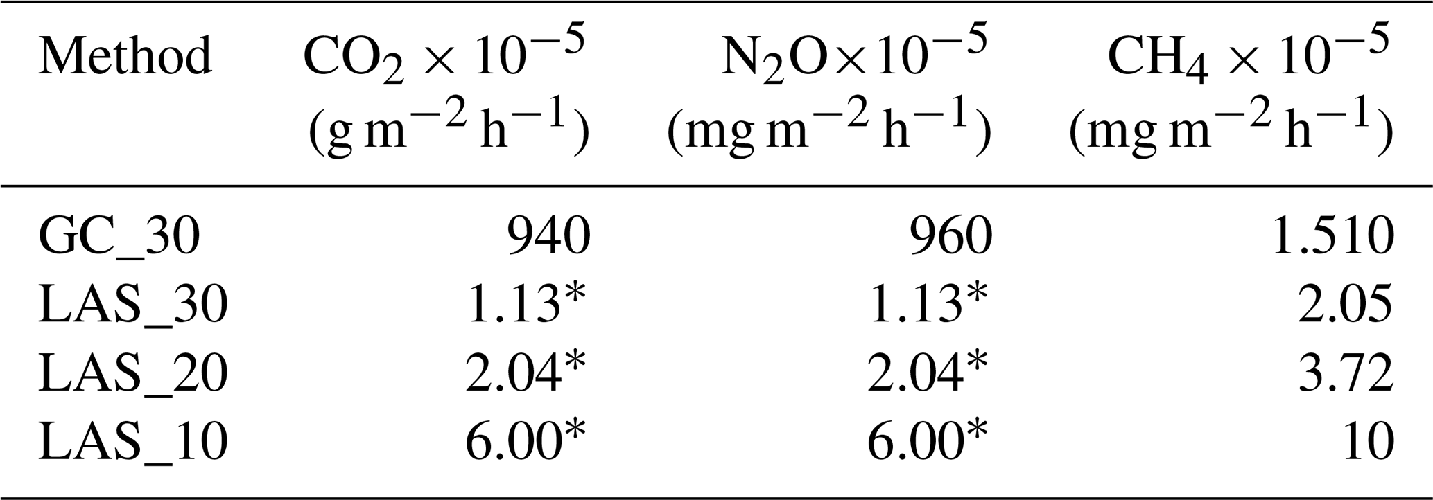
^* Identical values for CO₂ and N₂O result from the analytical precision of the instruments (200 ppb for CO₂, 0.2 ppb for N₂O) and the very similar molar masses of both gases. Therefore, the differences are only reflected in the units, not in the actual values.

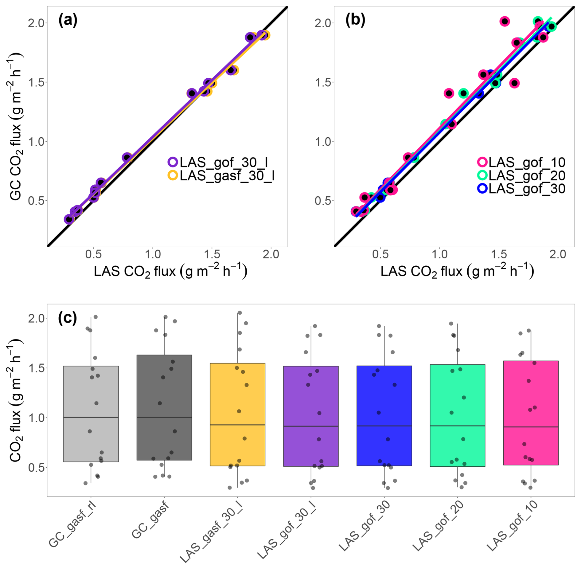
Figure 2 Comparison of CO₂ fluxes derived from gas chromatography (GC) and mid-infrared laser absorption spectroscopy (LAS) measurements using different chamber closure durations and calculation approaches. (a) GC derived fluxes for a 30 min chamber closure duration, calculated using the gasfluxes script with robust linear regression (GC_gasf_rl), are plotted against LAS derived fluxes also for a 30 min closure duration. The LAS fluxes were calculated using either the gasfluxes script (LAS_gasf_30_l) or the goFlux script (LAS_gof_30_l), both with linear regression. (b) Model-selected GC fluxes for a 30 min closure duration using the gasfluxes script (GC_gasf_30) are compared to model-selected LAS fluxes using the goFlux script for 30, 20, and 10 min enclosure durations (LAS_gof_30, LAS_gof_20, LAS_gof_10). In both panels (a) and (b), the black line represents the line of equality, while coloured lines indicate regression lines for the respective approaches. For CO₂, all flux values exceeded the minimum detectable flux (MDF). (c) Boxplots of all calculated CO₂ fluxes across methods and durations (n=16). For the summary of the mathematical analysis underlying the scatter plot comparisons, see Table 2.

Table 2 Regression results comparing CO₂ fluxes derived from Gas Chromatography (GC) and mid-infrared laser absorption spectroscopy (LAS) with varying chamber closure times and calculation scripts. Displayed are the correlation coefficient (r), regression equation, root mean square error (RMSE), and normalized RMSE (nRMSE).

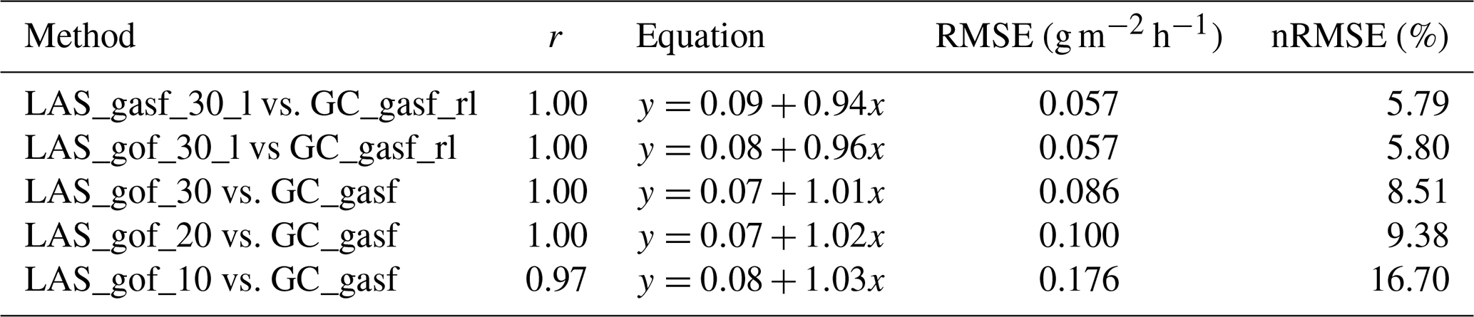
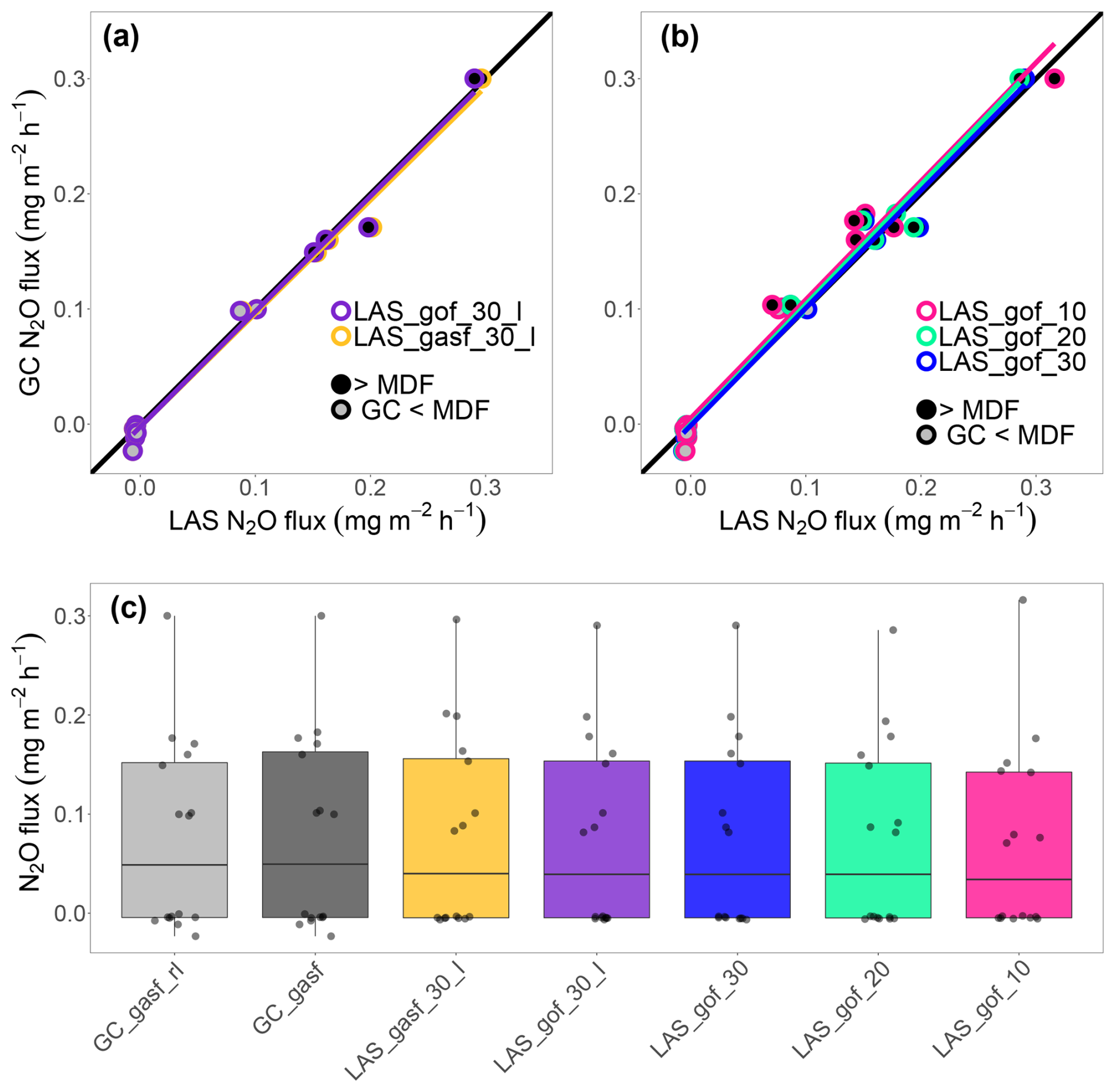
Figure 3 Comparison of N₂O fluxes derived from gas chromatography (GC) mid-infrared laser absorption spectroscopy (LAS) measurements using different chamber closure durations and calculation approaches. (a) GC derived fluxes for a 30 min chamber closure duration, calculated using the gasfluxes script with robust linear regression (GC_gasf_rl), are plotted against LAS derived fluxes also for a 30 min closure duration. The LAS fluxes were calculated using either the gasfluxes script (LAS_gasf_30_l) or the goFlux script (LAS_gof_30_l), both with linear regression. (b) Model-selected GC fluxes for a 30 min closure duration using the gasfluxes script (GC_gasf_30) are compared to model-selected LAS fluxes using the goFlux script for 30, 20, and 10 min enclosure durations (LAS_gof_30, LAS_gof_20, LAS_gof_10). In both panels (a) and (b), the black line represents the line of equality, while coloured lines indicate regression lines for the respective approaches. For N₂O, only higher fluxes exceeded the minimum detectable flux (MDF) (points filled in black), whereas all LAS flux values exceeded the MDF (points filled in grey). (c) Boxplots of all calculated N₂O fluxes across methods and durations (n=16). For the summary of the mathematical analysis underlying the scatter plot comparisons, see Table 3.

For N₂O, a generally good agreement was also observed between the flux values derived from GC and LAS flux estimation (Fig. 3, Table 3). This was observed both, without (Fig. 3a) and with the flux selection procedure (Fig. 3b). For N₂O, flux selection for LAS fluxes calculated with the goFlux script always resulted in HMR models. In contrast, model selection for GC fluxes using the gasfluxes script was only possible for 25 % of the fluxes due to the absence of HMR and kappa values, as a result of the script's internal HMR diagnostics. The flux selection algorithm resulted in HMR model fits for 19 % of these fluxes. Notably, obtaining HMR models with GC fluxes was only possible on the first measurement day, when an N₂O emission pulse occurred. The values cover a range of flux magnitudes, including very low and higher values. The data points align closely along the line of equality, and only a few GC measurements fell below the MDF (low flux range), whereas all LAS fluxes (even small negative fluxes) were above the MDF. The median flux magnitudes were relatively similar overall, with the GC fluxes tending to be higher, as was also observed for CO₂. The nRMSE varied between 14.63 % and 24.64 %, with the highest values corresponding to the shortest LAS closure time (10 min), as also observed for CO₂.

Table 3 Regression results comparing N₂O fluxes derived from Gas Chromatography (GC) and mid-infrared laser absorption spectroscopy (LAS) with varying chamber closure times and calculation scripts. Displayed are the correlation coefficient (r), regression equation, root mean square error (RMSE), and normalized RMSE (nRMSE).

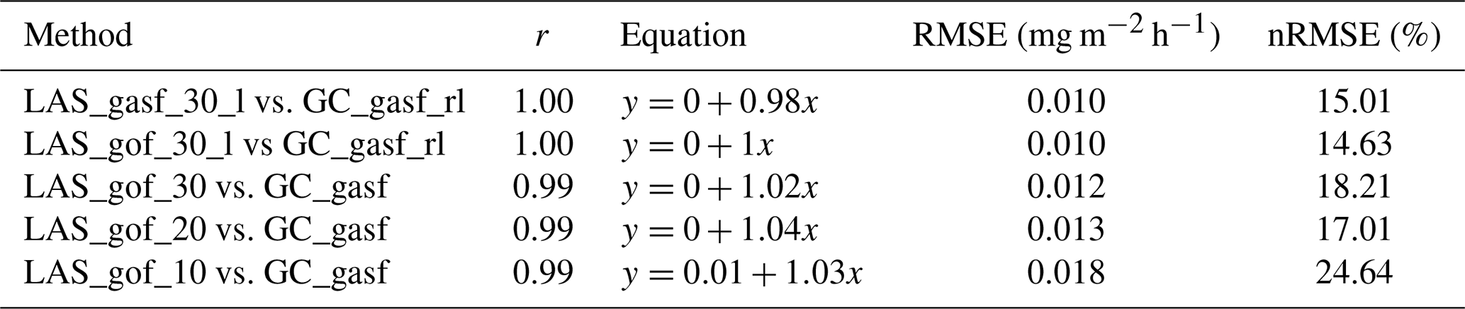
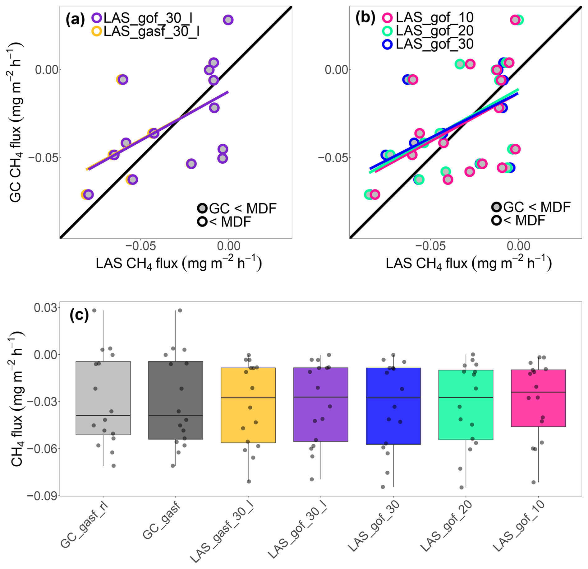
Figure 4 Comparison of CH₄ fluxes derived from gas chromatography (GC) and mid-infrared laser absorption spectroscopy (LAS) measurements using different chamber closure durations and calculation approaches. (a) GC derived fluxes for a 30 min chamber closure duration, calculated using the gasfluxes script with robust linear regression (GC_gasf_rl), are plotted against LAS derived fluxes also for a 30 min closure duration. The LAS fluxes were calculated using either the gasfluxes script (LAS_gasf_30_l) or the goFlux script (LAS_gof_30_l), both with linear regression. (b) Model-selected GC fluxes for a 30 min closure duration using the gasfluxes script (GC_gasf_30) are compared to model-selected LAS fluxes using the goFlux script for 30, 20, and 10 min enclosure durations (LAS_gof_30, LAS_gof_20, LAS_gof_10). In both panels (a) and (b), the black line represents the line of equality, while coloured lines indicate regression lines for the respective approaches. For CH₄, no GC flux values exceeded the minimum detectable flux (MDF), while almost all LAS flux values did (points filled in grey). Only one LAS flux fell below the MDF (indicated by an empty fill, located in the top right corner). (c) Boxplots of all calculated CH₄ fluxes across methods and durations (n=16). For the summary of the mathematical analysis underlying the scatter plot comparisons, see Table 4.

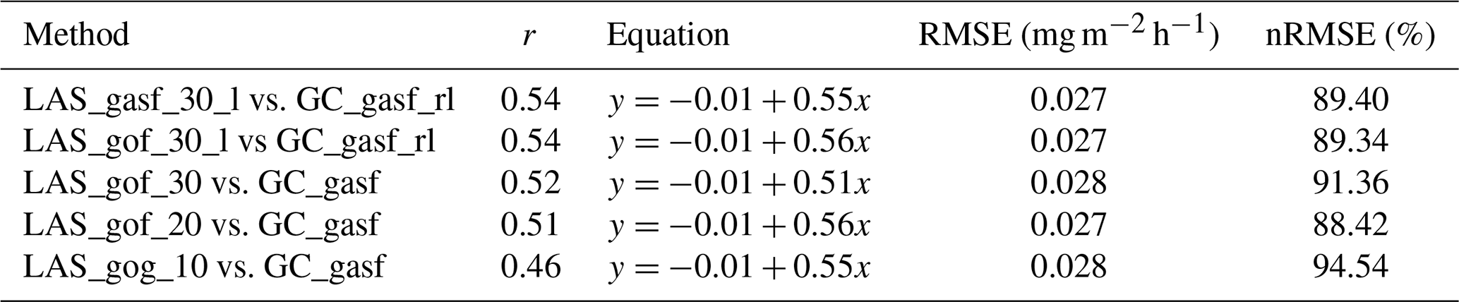
Figure 4 illustrates the comparison of CH₄ fluxes between GC and LAS methods without (Fig. 4a) and with model selection (Fig. 4b). In contrast to CO₂ and N₂O, the data points displayed substantial scatter, and the agreement with the line of equality was visible weaker (compare to Figs. 2 and 3) and the nRMSE values remarkable higher (compared to Tables 2 and 3). For CH₄, flux selection for LAS fluxes calculated with the goFlux script always resulted in HMR models. In contrast, model selection for GC fluxes using the gasfluxes script was only possible for 50 % of the fluxes due to the absence of HMR and kappa values, as a result of the script's internal HMR diagnostics. The flux selection algorithm resulted in HMR model fits for 13 % of these fluxes. Despite some spread, the flux value distributions across GC and LAS measurements appear broadly similar (Fig. 4c), without significant differences between the approaches, although the median of the GC data tended to be higher (more negative). All GC fluxes were below the MDF, whereas nearly all LAS fluxes except for one value with 10 min enclosure time were above it. The regression analysis confirmed the visual impression of lower consistency. The correlation coefficients (r) remained ≤0.54 in all cases and the nRMSE values ranged between 88.42 % and 94.54 %, indicating relatively large relative deviations (Table 4).

Table 4 Regression results comparing CH₄ fluxes derived from GC and LAS methods with varying chamber closure times and calculation scripts. Displayed are the correlation coefficient (r), regression equation, root mean square error (RMSE), and normalized RMSE (nRMSE).

4 Discussion

Overall, the measurement setup proved suitable for a method comparison, enabling the detection of both high and low flux magnitudes for CO₂ and N₂O. The CH₄ oxidation rates covered the common range for arable soils (Le Mer and Roger, 2001), further supporting the suitability of the dataset for the method comparison across all three gases. While treatment effects (two treatments) were tested, none were statistically significant and therefore not investigated in further detail. The calculation of the MDF according to Nickerson (2016) revealed marked differences between the GC and LAS methods, which can be attributed to substantial disparities in analytical precision. As a result, the LAS method was able to detect significantly lower fluxes than the GC method, representing a clear analytical advantage. The LAS-method's high sensitivity allowed for the detection of fluxes that would have remained below the detection threshold of the GC and would therefore have been classified as not significantly different from zero. Consequently, the enclosure time could be reduced substantially (e.g., to 10 min), as also recommended in other studies (Brümmer et al., 2017), without leading to a strong increase in the MDF, offering additional methodological flexibility and potential reduction of measurement duration-induced disturbances.

For CO₂, a high level of agreement was observed between the GC and LAS data pairs across all chamber durations and both scripts (gasfluxes and goFlux). The MDF was exceeded in all cases for both LAS and GC, facilitating comparability. Absolute flux values did not differ significantly between approaches, and the nRMSE remained low across all comparisons (max. 17 %, see Table 2). The regression slopes were close to 1, and intercepts near zero, indicating that both systems reliably captured actual CO₂ fluxes under field conditions. In line with Cowan et al. (2025), this shows that the common and still widely employed closed static chamber method is not necessarily inferior to closed dynamic chamber approaches in situations where the measured fluxes are considerably larger than the analytical uncertainty. For N₂O, the comparison revealed clear differences between the two measurement days. On the first day, flux magnitudes were relatively high, and MDF were exceeded by both methods. On the second day, however, flux magnitudes were low and, in some cases, negative. The fertilization in the crop rotation had taken place 17 months before the first measurement day and 23 months before the second measurement. We therefore consider it unlikely that the observed N₂O peak in our study was strongly influenced by earlier nitrogen inputs. Instead, it is more plausibly explained by mineralization pulses triggered by the series of soil tillage interventions carried out shortly before the first measurement day (see Sect. 2.2), of course in combination with long-term effects of earlier nitrogen inputs. The capture of this N₂O pulse, along with the very low to negative fluxes, demonstrated a strong agreement between methods, with only minimal error for the 30 min enclosure time (nRMSE: 15 %) and a tolerable deviation for 10 min enclosure time (25 %) (see Table 3). Negative fluxes were consistently detected and quantified by the LAS method, whereas the GC measurements for these fluxes fell below the MDF, resulting in no significant difference from zero flux. This demonstrates the superior ability of LAS to measure very low N₂O fluxes and even small net uptake events. Such negative fluxes are commonly attributed to the final step of denitrification, where N₂O is reduced to N₂ (Cavigelli and Robertson, 2001; Glatzel and Stahr, 2001; Butterbach-Bahl et al., 2002). Although these processes are well documented, they are frequently underestimated or omitted in flux datasets, as negative net fluxes often fall below detection thresholds. Chapuis-Lardy et al. (2007) highlight that this omission may lead to critical misinterpretations of the global N₂O budget. The high analytical sensitivity of the LAS method could help to better integrate N₂O sinks, but also very low N₂O emissions into future flux assessments (Cowan et al., 2025; Triches et al., 2025).

The results for CH₄ showed considerable divergence. All measured LAS-derived CH₄ fluxes were negative, as were almost all GC-derived CH₄ fluxes, as expected for well-aerated arable soils where CH₄ oxidation by methanotrophic bacteria predominates (Hütsch, 1998; Powlson et al., 2014). While the LAS measurements consistently exceeded the MDF, the GC fluxes did not, likely resulting in a higher degree of uncertainty in the GC dataset and thus a lower ability to detect potential treatment effects in CH₄ consumption rates. This discrepancy may have led to inflated variability in the GC results, particularly at low flux values (near zero). Even under conditions with only low changes in CH₄ concentrations, the LAS provided significant results (flux > MDF) for nearly all fluxes (with only one exception, with a 10 min chamber enclosure time), highlighting its advantage in terms of flux sensitivity. Despite these differences and the low agreement of measured fluxes, the mean CH₄ fluxes did not differ significantly between methods (see Fig. 4c), suggesting that any potential effects induced by treatment factors might be captured in a similar manner. For verification of the assumption, both with GC and LAS, measuring a time series with different treatments and calculating cumulative fluxes is advisable. However, the low correlation (r≈0.5) and high nRMSE up to 95 % indicate that more extensive datasets with more values exceeding MDF for GC fluxes are needed to validate this assumption. Even so, according to Le Mer and Roger (2001), CH₄ oxidation rates in aerobic upland soils rarely exceed 0.1 mg m⁻² h⁻¹. In our case, we observed rates up to 0.08 mg m⁻² h⁻¹. This leads us to assume that a more extensive dataset of simultaneous chamber measurements would probably not have provided further clarity, as our values were already close to this typical upper limit. For further investigations, reducing effective chamber height may represent the most effective measure to minimize MDF. However, in field campaigns, this approach is often not feasible, as it is often of interest to include plants within the chamber (e.g. Flessa et al., 2002; Zhang et al., 2013) and also to level out spatial variability over capturing larger soil surface area (e.g. heterogeneous distribution of solid manure and composts, Krauss et al., 2017). In our study, we used our standard chamber configuration, which is relatively high and generally applied in the LTE at the study site, where tall crops are frequently grown. While our relatively large effective chamber height (0.68 m) increased the MDF, our results show that CH₄ fluxes above the MDF could still be detected with the LAS system, whereas this was not possible with the GC-based approach. This means that, because CH₄ consumption rates in arable soils are generally very low, measurements made with large effective chamber height often yield fluxes below the MDF with GC method.

For chamber-based flux measurements, three types of water vapor corrections need to be considered: (i) absorption band broadening, (ii) instrument cross-sensitivity, and (iii) dilution of the air sample by water vapor. The dry trace gas values reported by the LAS are automatically corrected for the first two effects, which are instrument-specific and implemented in the LAS software. However, the third effect, the dilution of the chamber air due to changes in water vapor concentration, is not corrected internally and must be applied by the user. This additional correction is included in the goFlux script, which is why it was applied in our data processing workflow. We calculated LAS fluxes both with and without water correction and compared them among each other as well as to the non-water-corrected GC fluxes. The application of the goFlux script, including correction for water vapor inside the chamber during the measurement (dilution effect) (Hupp and McDermitt, 2012), had only marginal effects on the absolute flux magnitudes and on the agreement between methods. This suggests that, in the present dataset, absolute humidity had little impact on flux calculations, despite noticeable differences between measurement days (average absolute humidity during each measurement day: 12.01 g m⁻³ on 21 September 2023 and 5.62 g m⁻³ on 25 March 2024). This is in contrast to Kong et al. (2025), who compared GC with a LI-COR LI-7820 N₂O/H₂O trace gas analyzer (LI-COR Biosciences, USA) based on optical feedback cavity-enhanced absorption spectroscopy (OF-CEAS) employing a near-infrared (NIR) tunable diode laser source: The authors applied water vapor corrections for dynamic chamber approach resulting in a significant effect on N₂O fluxes, especially below 50 µg N₂O-N m⁻² h⁻¹ (0.079 mg N₂O m⁻² h⁻¹, own conversion). This contributed to discrepancies in cumulated N₂O emission estimates in a similar chamber-based method comparison campaign on Danish arable soils. They explained this discrepancy mainly by the different enclosure times. In contrast to our experimental design, enclosure times were not the same for the two different measurement modes. The dynamic chambers, used with the OF-CEAS, had much shorter enclosure times (2 to 16 min), which minimized the effect of water vapor changes, whereas static chambers used for GC sampling remained closed for 45 to 110 min and concentrations measurements were typically not corrected for water vapor at all. Additionally, there might have been a seasonal effect. The experiment of Kong et al. (2025) which was most similar in design to our experiment was conducted during the summer (June until September). The largest water vapor dilution effects occur on wet soils and/or soils with strongly transpiring plants at low CO₂ fluxes under dry and sunny conditions. The latter can lead to strong increases in chamber air temperature and subsequently in chamber humidity when a moisture source is available (Welles et al., 2001).

The flux selection approach was applied according to Hüppi et al. (2018) for both LAS and GC fluxes. While HMR models were selected in all cases for the LAS fluxes, the gasfluxes script limited HMR calculations for GC fluxes to a subset (CO₂: 31 %, N₂O: 25 % and CH₄: 50 %), as most fluxes did not meet the criteria defined by the internal HMR diagnostics of the script. Based on this subset, the flux selection algorithm selected HMR models for an even smaller fraction of the GC fluxes (CO₂: 31 %, N₂O: 19 %, CH₄: 13 %). On the first measurement day, when a high N₂O emission peak occurred, 3 out of 8 N₂O fluxes could be calculated using the HMR model, while on the second measurement day, however, none could be fitted with HMR. This illustrates that applying HMR calculations to GC-based measurements is often problematic, particularly at very low flux magnitudes near the MDF. It remains unclear whether this is primarily due to the limited number of measurement time points (only six per chamber) or the lower analytical precision of the method, or a combination of both. Although the gasfluxes script's internal HMR diagnostics allowed significantly more HMR model calculations for LAS compared to GC fluxes, it somewhat surprisingly still did not provide HMR models for all LAS fluxes, unlike the goFlux script. Nevertheless, when comparing the two methods (GC and LAS) with and without flux selection, it became apparent that there was only a small influence of the model selection procedure on our results and it did not significantly affect the relationship between the two methods over the 30 min closure periods. In contrast, the shorter chamber closure durations had a more pronounced effect on the flux estimates. The relative error for CO₂ and N₂O was highest with the LAS when using a 10 min closure time, compared to the GC fluxes, which were always based on a 30 min enclosure. However, even in this case, the error remained within a moderate range for these two gases. Also, for CH₄, reducing the enclosure time to 20 and 10 min had only a minimal effect on the calculated LAS-derived fluxes. In addition to the only slightly reduced MDF resulting from the shortened chamber enclosure durations (see Table 1), this further highlights the LAS method's suitability in terms of operational practicability and the reduction of measurement duration-induced disturbance of the gas concentration gradient and hence gas flux dynamics between soil and chamber atmospheres. Given the amount and quality of data that LAS analyzers can provide, a suitable alternative approach might be the use of a generalized additive model for calculating fluxes from individual chamber measurements (Themistokleous et al., 2024), which is recommended for future assessments of LAS data. Taken together, although no treatment effects were explicitly tested in this study, both GC and LAS approaches resulted in comparable flux magnitudes for CO₂ and N₂O, suggesting that both methods would very likely provide consistent results when assessing potential treatment effects. For CH₄, flux magnitudes also did not differ significantly between methods; however, this apparent agreement is subject to considerably greater uncertainty, as indicated by the scatterplot analysis and the fact that GC fluxes were generally below the MDF and thus not significantly different from zero flux. However, for all three gases, a pattern of slightly higher fluxes, measured by GC, was observed. This slight pattern should not be overinterpreted. For CO₂, the confidence is by far the highest, as all GC values are above the MDF, even though the median differences compared to LAS values are only slight (Fig. 2c). For N₂O, the differences in medians (Fig. 3c) are even smaller, and the confidence is lower because the small estimated GC fluxes for N₂O are less reliable (< MDF). For CH₄, the median deviation between GC and LAS values is largest (Fig. 4c), but almost all GC CH₄ values (except one) fall below the MDF. Regarding CO₂, Christiansen et al. (2015a) reported that at very high CO₂ concentrations (>2000 ppm), GC measurements tended to overestimate gas concentrations compared to cavity ring-down spectroscopy (CRDS), which they attributed to the non-linear response of the detector (TCD). In our dataset, however, the highest measured CO₂ concentration is only 1337 ppm, well below the levels at which (Christiansen et al., 2015a) clearly observed this effect. Therefore, the exact cause of the slight overestimation in our CO₂ flux data remains unclear. Nevertheless, it is conceivable that the detector-related non-linearity reported by Christiansen et al. (2015a) could play a role, implying that GC-based CO₂ flux measurements may slightly overestimate fluxes under certain conditions.

The LAS offers several technical and analytical advantages: its low MDF allows for the detection of very small but significant CH₄ and N₂O fluxes; it permits shorter enclosure times without substantial increases in uncertainty; and it offers real-time measurements with minimal infrastructure requirements. These features enable faster, more flexible sampling and improve the resolution of short-term flux dynamics, such as during N₂O pulse-emission events. While analyzers are already used at long-term monitoring sites (e.g. ICOS Ecosystem Stations) (Pavelka et al., 2018) and have also been applied in field experiments using manual (e.g. Dix et al., 2024) or rarely automated chambers (Brümmer et al., 2017; Bond-Lamberty et al., 2020), their limited mobility makes such measurements logistically demanding and constrains spatial coverage and therefore limits the ability to capture spatial variability. Recent advances in LAS techniques have led to the development of smaller and more portable analyzers, which now make high-frequency flux measurements less challenging and more feasible over a broader spatial scale with manual chamber applications, including at plot or ecosystem scale. Our results demonstrate that these portable LAS systems can detect very small CH₄ and N₂O fluxes that are often below the detection limit of conventional GC-based approaches. Consequently, portable LAS analyzers represent an important methodological advancement and can substantially improve the accuracy of annual and long-term GHG budget calculations, especially with respect to CH₄ and N₂O.

Beside the methodological advantages there are practical limitations of the LAS like increased vulnerability to environmental influences (e.g. dust, moisture, high temperature), and maintenance demands, which may affect measurement logistics under field conditions. From an economic perspective, the purchase of LAS systems is generally reasonable, particularly when considering the operating costs of GC systems. Although GC systems offer clear advantages, such as the ability to easily conduct multiple measurement campaigns in parallel, the choice between GC and LAS ultimately depends on budgetary constraints and the specific requirements and aims of the study.

5 Conclusions

Biotic greenhouse gas (GHG) fluxes are often measured using the closed chamber method, but the choice of analytical instrumentation influences flux estimations and reliability of the results. In this study, we compared gas chromatography (GC) with mid-infrared laser absorption spectroscopy (LAS) based on simultaneous static (GC) and dynamic (LAS) chamber measurements and derived the following conclusions:

• The measurement days proved to be suitable for the comparison, as they covered a range of fluxes across the investigated gases (CO₂, CH₄, and N₂O) regarding arable soils.

• For CO₂ fluxes, a very high level of agreement between the methods was observed. All fluxes were well above the minimum detectable flux (MDF), and deviations were low (nRMSE ≤17 %), confirming the reliability of both methods for measuring CO₂.

• For N₂O, the methods showed strong agreement across both measurement days, with high correlation coefficients (r≈1) and low deviations (nRMSE ≤25 %). For low fluxes GC-derived fluxes fell below the MDF and could not be distinguished from zero flux.

• In the case of CH₄, the agreement between methods was poor (nRMSE up to 95 %). Covering the common range for CH₄ oxidation rates, none of the GC measurements exceeded the MDF. In contrast, almost all values measured by LAS exceeded the MDF, which likely contributed to the weak correlation between the two methods CH₄ fluxes.

• A central advantage of the LAS method lies in its considerably lower MDF due to the higher measurement frequency (∼1 Hz) and analytical precision, which enables the detection of statistically significant fluxes (flux > MDF) even at a very low flux range. This is especially relevant for CH₄ and N₂O, where small flux rates occur and uptake of either gases into the soil-plant system might remain undetected.

• Due to the considerably lower MDF of the LAS method, shorter chamber enclosure times are potentially possible, even at small flux rates. Our results confirmed this advantage, which showed that it is possible to reduce the chamber enclosure time to 10 min while obtaining similar results.

• The ability to visualize and validate measurements in real time adds to the practical benefits of LAS, offering increased flexibility in field campaigns. However, GC systems offer advantages, such as the ability to conduct multiple measurement campaigns in parallel.

Overall, this pilot study provides a comprehensive comparison of two widely used analytical techniques for chamber-based GHG flux measurements. Given the high agreement observed between methods for CO₂ and N₂O, we conclude that LAS is a valid and reliable alternative to the established GC approach for these gases. For quantifying CH₄ uptake rates in arable soils, there is considerable uncertainty regarding the consistency between the two methods; however, this is very likely due to the high MDF of the GC method. In conclusion, the LAS's analytical sensitivity and operational flexibility clearly supports its broader application in trace gas research, especially for gaining new insights into the natural variability of low soil GHG fluxes which are masked by instrumental noise of world-wide very common GC technique.

Appendix A: Details of standard gases for gas chromatography measurements

Table A1 List of (non-isotope) standards used for testing and calibration^*.

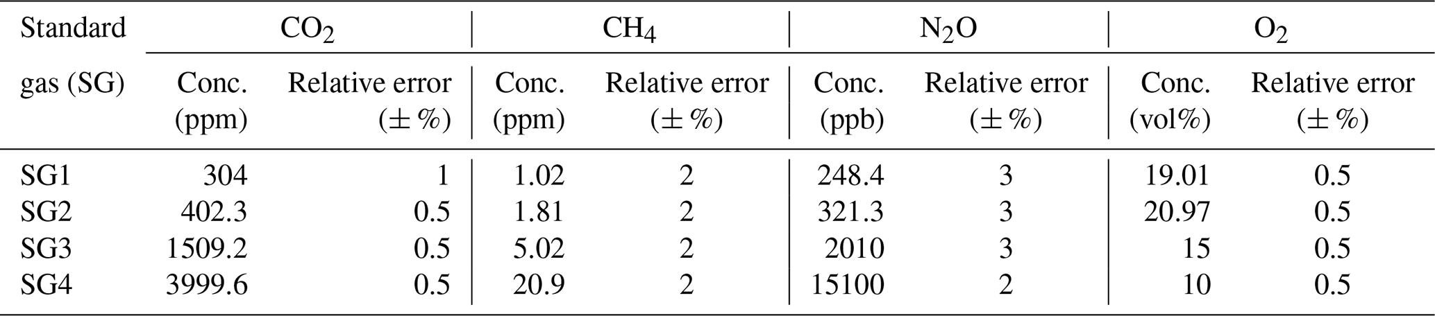
^* According to analysis certificate of the manufacturer (DEUSTE Steininger GmbH, DE).