Spatial and temporal variability of CO₂, N₂O and CH₄ fluxes from an urban park in Denmark

With the rapid worldwide increase in urbanization, urban green spaces are becoming increasingly important in regulating biogeochemical cycles and associated greenhouse gas (GHG) fluxes on regional and global scales. However, the existing data and research on the potential roles of urban green spaces remain limited. In this study, we conducted in situ measurements of nitrous oxide (N₂O) and methane (CH₄) fluxes, as well as ecosystem carbon dioxide (CO₂) respiration, at 56 sites in a temperate urban park with a hilly landscape during the vegetation-growing and frost-free period as well as the freeze–thaw period. Based on the arithmetic mean of all the measurements, the soil acted as a source of N₂O (23.8 ± 1.7 µg N m⁻² h⁻¹) and a weak sink of CH₄ (−0.26 ± 2.14 µg C m⁻² h⁻¹). Over the entire observation period, the mean ecosystem CO₂ respiration was calculated to be 228 ± 18.5 mg C m⁻² h⁻¹. High spatial and temporal variability was observed for all three GHG fluxes, with the coefficient of variation ranging from 45.6 %–259 % for N₂O, 3154 %–4962 % for CH₄ and 40.3 %–49.3 % for CO₂, respectively. This variability was primarily associated with changes in soil and environmental factors, including vegetation structure, soil hydrothermal conditions, pH, and the availability of soil carbon and nitrogen. Moreover, random forest models combining the in situ measured data and landscape parameters demonstrated a high probability of identifying spatial patterns and hot or cold spots of GHG fluxes across this heterogeneous landscape. However, the models' performance was limited by the lack of high-resolution soil and vegetation data. Overall, our study provides valuable insights into scaling GHG fluxes in urban green spaces more effectively, enabling a more accurate assessment of how urbanization changes landscape fluxes.

1 Introduction

Atmospheric carbon dioxide (CO₂), methane (CH₄) and nitrous oxide (N₂O) are the three important greenhouse gases (GHGs), that significantly impact global warming and atmospheric chemistry (Ravishankara et al., 2009; IPCC, 2013, 2021). Microbial processes in soil are major natural sources and sinks of these GHGs (Conrad, 1996; Smith et al., 2018). The strength of these biogenic sources and sinks varies greatly over space and time, and they are expected to respond to environmental and land use changes (van Delden et al., 2016; Feng et al., 2022). Due to rapid worldwide urbanization, soils of urban green spaces, such as urban parks, residential gardens, street trees and small wooded patches,are becoming increasingly significant as sources or sinks of these GHGs (van Delden et al., 2018; Zhan et al., 2023). However, in order to determine the realistic global warming potential of soils of urban green spaces, the fluxes of all three GHGs must be accurately quantified and scaled up. Moreover, identifying the drivers of variability in the source/sink strength of these GHGs is also critical for predicting how soils of urban green spaces will respond to climate change in the future.

Compared with natural forests, grasslands, and managed agricultural systems, urban ecosystems may exhibit distinct biogeochemical C and N cycles due to the complex interactions between society and the environment (Kaye et al., 2006). These interactions may result in unique characteristics of CO₂, CH₄ and N₂O fluxes from urban green spaces. However, most previous studies on soil GHG fluxes have mainly focused on forests, grasslands, and agricultural ecosystems (Gao et al., 2022; Wangari et al., 2022; Liu et al., 2025; Walkiewicz et al., 2025). Existing studies on GHG fluxes in urban ecosystems have primarily examined CO₂ exchange; while urban soil N₂O and CH₄ fluxes remain poorly characterized (Jeong et al., 2024; Karvinen et al., 2024; Pan et al., 2024). Braun and Bremer (2018) reported that annual N₂O emissions from various fertilized urban green spaces were between 1.0 and 7.6 kg N ha⁻¹ yr⁻¹, comparable to emissions from intensive agriculture. Despite covering only 6.4 % of the investigated land area, Kaye et al. (2004) suggested that urban lawns contribute up to 30 % to regional N₂O budgets. A literature review by Zhan et al. (2023) revealed that soils of urban green spaces generally act as a sink for atmospheric CH₄, with an average annual uptake of 2.0 kg C ha⁻¹ yr⁻¹. However, this magnitude is relatively low compared to the annual CH₄ uptake by other non-urban soils and would decrease further with increased urbanization (Zhang et al., 2021). Although urban green spaces are often overlooked, existing studies indicate that they can influence regional and global climate change by increasing N₂O emissions and reducing soil CH₄ uptake.

Urbanization involves a transition from natural and managed ecosystems to urban green spaces, which alters environmental and soil conditions, such as soil texture, pH, nutrient availability and hydrothermal dynamics (Kaye et al., 2006; Edmondson et al., 2016; Zhan et al., 2023). These factors, acting alone or in combination, lead to high spatial and temporal variability in soil GHG fluxes. This variability limits the ability of researchers to constrain regional and global emission inventories. Currently, the uncertainty associated with most estimates of GHG fluxes from urban soils is often substantial, as the spatial and temporal variations of urban soil fluxes are not well understood. Furthermore, such high uncertainty hinders the identification of the primary drivers of spatiotemporal variability. Nonetheless, machine learning approaches such as random forest models can be used to effectively identify the key environmental factors driving the spatiotemporal variability of soil GHG fluxes. Many studies have used random forest models incorporating soil, climate and management factors to predict GHG flux dynamics in various ecosystems, such as grasslands (Barczyk et al., 2024), wetlands (Ying et al., 2025), and agricultural fields (Saha et al., 2021).

Denmark, which consistently ranks among the top three happiest nations in international well-being surveys, has a higher per capita provision of urban green spaces (61.7 m² per capita) than the global average (Statistics Denmark, 2025). This provides a valuable opportunity to examine the biogeochemical significance of urban green spaces for humans and the environment. Numerous studies have emphasized the various ecosystem services provided by urban green spaces, such as environmental services (e.g., mitigating elevated urban heat and pollution), ecological services (e.g., sustaining urban wildlife habitats and biodiversity conservation), and social and human health benefits (Cardinali et al., 2024; Poulsen et al., 2024). However, no studies have yet reported measurements of in situ soil GHG fluxes from urban green spaces in Denmark. Therefore, the aim of this study was to quantify and characterize the spatial and temporal variability of soil N₂O, CH₄ and CO₂ fluxes, using a large number of sampling sites (n=56) spread across an urban park in Aarhus, Denmark. Furthermore, we assessed the role of environmental and soil variables (e.g., topography, soil temperature, moisture, soil organic C, total N and pH) as the main drivers of these spatiotemporal patterns. We also used a machine learning-based upscaling framework to predict the potential GHG hot spots and cold spots.

2 Materials and methods

2.1 Study area

The study area is located within the 8.2 ha Aarhus University Park (AU Park) in the center of Aarhus, Denmark (56.168° N, 10.203° E) (Fig. 1). The region has a temperate oceanic climate (Cfb, Köppen classification), which is characterized by warm and humid summers and cold and damp winters. The area's long-term average annual precipitation is 1046.3 mm, and its mean annual temperature is 8.8 °C (Danish Meteorological Institute, http://www.dmi.dk, last access: 5 March 2025). Mean daily temperatures range from a minimum of −14.6 °C to a maximum of 26.4 °C, with frequent frost occurring in the winter months. AU Park is situated in a hilly landscape that is part of an old moraine valley extending from Katrinebjerg in Vejlby in the north to the Bay of Aarhus in the east. The park area is dominated by grass-clover lawns that are occasionally mowed and interspersed with old oak trees (Quercus robur) that are over 80 years old. Two artificial ponds have been created in the lower part of the park and are fed by a small stream that comes from a spring inside the park.

To better understand the spatial and temporal variability of CO₂, CH₄ and N₂O fluxes, 56 sampling sites were selected across the AU Park using a stratified random sampling design. The sites were stratified based on their landscape position and proximity to ponds to effectively capture spatial heterogeneity in vegetation types, microtopography and soil moisture conditions. For example, more sampling sites were established in areas with apparent topographic changes, while fewer sampling sites were set up in areas with flat and homogeneous vegetation.

The soils in the study area are typically Luvisols (Adhikhari et al., 2014), with a sandy loam to loamy texture in the topsoil that developed on moraine sand (Pedersen et al., 1989). However, since AU Park is surrounded by university buildings established in the 1930s and a full soil survey was beyond the scope of this study, we assume that the park's soils have been affected by the incorporation of building materials and landscaping. This has resulted in altered soil profiles and soil properties compared to “natural” soils (Vasenev and Kuzyakov, 2018). No fertilizer was applied during the measurement periods.

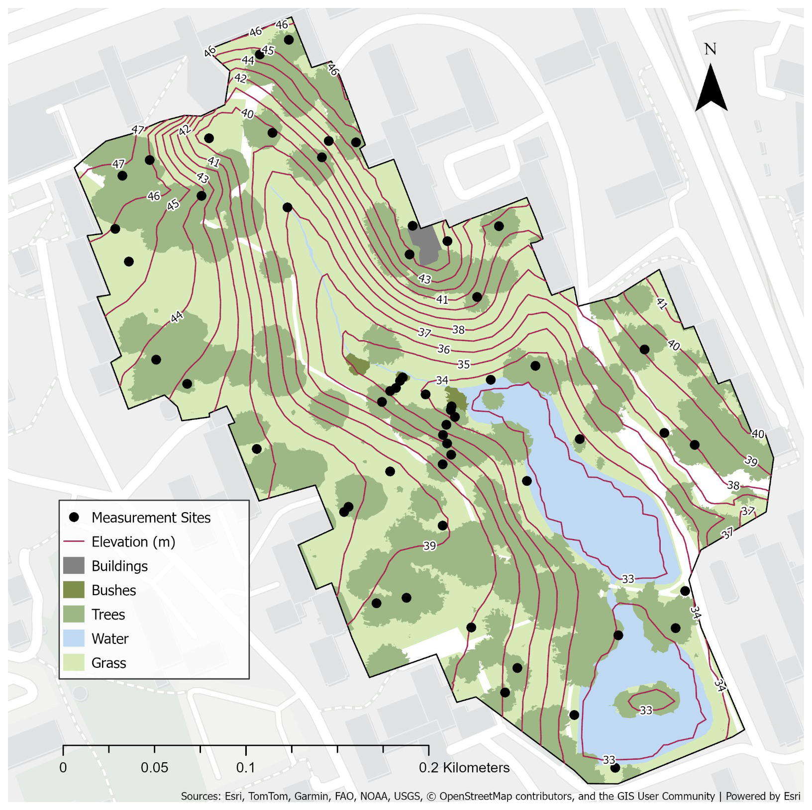
Figure 1 The map showing the land cover types and the locations of the sampling sites across a city park at Aarhus University.

2.2 Measurements of CO₂, CH₄ and N₂O fluxes

Fluxes of CO₂, CH₄ and N₂O were measured using the fast-closed chamber technique, as described by Hensen et al. (2013) and Daelman et al. (2025). The opaque chamber was 20 cm high and 37.5 cm in diameter. It contained a small fan inside to mix the air in the chamber and a 1 m long, 3.2 mm wide ventilation tube at the top of the chamber for pressure equalization. Instead of using pre-installed ground frames, we carefully pushed the chamber, with its sharpened and polished bottom edge, about 1–2 cm directly into the ground for flux measurements. To ensure that each flux measurement was always taken from the same plot at the sampling site, we inserted a small metal plate (approximately 1 × 1 cm) into the soil and used a metal detector to locate the plate and identify the site.

During the vegetation-growing and frost-free period (20 July to 9 November 2023) and the freeze-thaw period (22 November to 7 December 2023), flux measurements were performed across all 56 sampling sites, using two portable infrared gas analyzers: one measuring N₂O concentrations (LI-7820, LI-COR Biosciences, Lincoln, NE, USA) and the other measuring CH₄ and CO₂ concentrations (LI-7810, LI-COR Biosciences, Lincoln, NE, USA) (Fig. S1). Here, the start and end dates of the vegetation-growing and frost-free period were determined based on daily mean air temperatures that consistently remained above 0 °C (Fig. 2). The freeze–thaw period was defined by the onset of repeated temperature fluctuations around 0 °C, resulting in alternating freezing and thawing conditions. Moreover, snow events occurred during the freeze-thaw period, with the cover depth ranging from approximately 0.1 to 13.1 cm. On each sampling day (08:00–16:00 CET), we used a chamber closure time of 5–7 min, and we monitored the change in headspace GHG concentrations by circulating headspace air between the chamber and the analyzers at a rate of approximately 200 mL min⁻¹. To minimize the potential impact of sampling, the sampling sites were monitored in a random order on each sampling date. Fluxes with units mass N m⁻² h⁻¹ for N₂O and mass C m⁻² h⁻¹ for CH₄ and CO₂ were then calculated based on the decrease or increase of headspace GHG concentrations over time using Eq. (1), which combines the ideal gas law and scaling variables:

$$\begin{array}{}\text{(1)}& F={\displaystyle \frac{\mathrm{d}q}{\mathrm{d}t}}\cdot {\displaystyle \frac{P\cdot V\cdot M}{R\cdot T\cdot A}}\end{array}$$

Where $\mathrm{d}q/\mathrm{d}t$ represents the rate of change of gas mixing ratios with time (h⁻¹), P is the atmospheric pressure (atm), V is the volume of sampling chamber (m³), M is the molar mass of the gas (mass mol⁻¹), R is the universal gas constant (m³ atm K⁻¹ mol⁻¹), T is the air temperature (K), and A is the area of sampling chamber (m²). The minimum detection limits of gas fluxes are 1.1 µg N m⁻² h⁻¹ for N₂O, 0.71 µg C m⁻² h⁻¹ for CH₄ and 4.1 mg C m⁻² h⁻¹ for CO₂, respectively. Note that the CO₂ emissions represent ecosystem respiration (ER-CO₂) because all above-ground biomass was trapped in the opaque chambers during the measurements, so the measured changes in chamber headspace CO₂ concentration were due to both soil and plant respiration.

During the entire observation period, we conducted gas sampling at least once per week, unless interrupted by logistical (holidays) and operational (e.g., instrument breakdown) constraints. Specifically, from 7 July to 1 September 2023, we measured fluxes one to three times per week. For the rest of the observation periods, the sampling frequency was reduced to once per week. In addition to measuring gas fluxes, a combined temperature and moisture HOBO sensor (MX2307, Onset, Bourne, MA, USA) was used to simultaneously record soil temperature and volumetric water content at a depth of 5 cm in the direct vicinity of each sampling chamber site.

2.3 Soil sampling and properties

At the end of the experimental period, topsoil samples (0–10 cm) were collected from the center of each sampling site using a soil auger. Part of the soil samples were used to measure soil ammonium (NH${}_{\mathrm{4}}^{+}$) and nitrate (NO${}_{\mathrm{3}}^{-}$) concentrations. After extraction of fresh soil samples with 1 M potassium chloride (KCl) solution in a soil:solution ratio of 1:2, soil NH${}_{\mathrm{4}}^{+}$ and NO${}_{\mathrm{3}}^{-}$ concentrations were analyzed using an AA500 AutoAnalyzer (Seal Analytical) (Best, 1976; Crooke and Simpson, 1971). Part of the soil samples were dried (60°, 48 h) and sieved (<2 mm) for later analyses of soil total nitrogen (TN), soil organic carbon (SOC) and soil texture. TN was analyzed by dry combustion using a Vario MAX cube (Elementar Analysensysteme AG, Langenselbold, Germany) (Nyang'au et al., 2023). Soil pH was measured in a soil solution with deionized water (soil:solution = 1:2) using a pH meter (3110 SET SM Pro, Xylem Analytics Germany GmbH) (Schofield and Taylor, 1955). The clay fraction (<2 µm) and silt fraction (2-20 µm) were quantified using the hydrometer method. Sand particles larger than 63 µm were separated through wet sieving and SOC was measured using high-temperature dry combustion (Schjønning et al., 2023). Besides, soil bulk density (BD) was measured using soil cores and weight measurements of oven-dried soil (105°, 24 h) (Alletto and Coquet, 2009).

2.4 Identification of hot and cold spots of GHG fluxes

In this study, the different subsections of the park were classified into three categories (hot spot, cold spot and normal spot) based on the relative magnitude of observed GHG fluxes.

The hot and cold spot thresholds were determined using a formula proposed by Gachibu Wangari et al. (2023). This formula provides a context-sensitive approach to categorising GHG fluxes by adapting to local conditions rather than relying on fixed absolute thresholds. The classification method was based on the median and interquartile range of the data by Eqs. (2) and (3):

$$\begin{array}{}\text{(2)}& {\displaystyle }\text{Hot spot threshold}=M+\left(\mathrm{Q}\mathrm{3}-\mathrm{Q}\mathrm{1}\right)\text{(3)}& {\displaystyle }\text{Cold spot threshold}=M-\left(\mathrm{Q}\mathrm{3}-\mathrm{Q}\mathrm{1}\right)\end{array}$$

where M is the median and Q3–Q1 is the interquartile range of the measured daily GHG fluxes from individual sampling sites during the vegetation-growing and frost-free period. Due to the skewed distributions of ER-CO₂ and N₂O fluxes, the thresholds were such that there were no cold spots. Here, CH₄ fluxes can be positive or negative values, representing a source of atmospheric CH₄ or a sink of atmospheric CH₄, respectively. Hence, hot spots were areas of high CH₄ emissions, and cold spots were areas of high CH₄ uptake. Neither hot spots nor cold spots were classified as normal spots for GHG fluxes.

2.5 Hot and cold spot upscaling

The hot and cold spots of GHG fluxes observed in the AU Park were upscaled using a random forest (RF) model through a two-step approach (Fig. S2).

First, the counts of hot, cold, and normal spots varied substantially across the three gases, with the normal spots category being predominant. This imbalance could potentially introduce biased sample numbers of training data under different categories, thus causing the RF model favoring the majority class and failing to accurately identify the minority classes. To address this issue, the minority categories were oversampled during training. We used an ad hoc, iterative approach to identify the most effective inflation factor of oversampling for each GHG (Tables S1–S3). Second, we used RF for classification with potential predictors of GHG fluxes, including soil physio-chemical properties, vegetation and topography (Table S4). The dataset was randomly divided into a training and internal cross-validation (80 %) and external test (20 %) sets using a stratified random sampling method. The models were trained and internally validated via 10-fold cross-validation (k=10) performed on the training dataset. We hyper-tuned the models for each GHG using a grid search (Tables S5) according to the log loss. Log loss was selected as a measure of how well the predicted probabilities matched the actual class labels, considering both prediction accuracy and confidence.

After hyper-tuning the model, the best performing model was used to rank the different predictors according to their importance (Tables S6–S8). This model was then used for feature selection, during which the least essential variables were removed stepwise according to their rank importance.

Lastly, the hot and cold spots were spatially upscaled for each GHG, using the final hyper-tuned model (after feature selection) at a monthly time step with a spatial resolution of 0.4 m. To do so, we aggregated the average monthly observations, while also interpolating soil physio-chemical and vegetation predictors using either ordinary kriging or inverse distance weighting for dynamic and temporally static predictors (Table S4). We aggregated all gridded predictors and used the hyper-tuned model to predict the total average classification probability. This created an average probability map showing the likelihood that a location would be classified as a hot spot or cold spot.

2.6 Statistical analysis

The daily fluxes of CH₄, N₂O and ER-CO₂ (ER: Ecosystem Respiration) for each sampling date were calculated as the mean of all observed fluxes from the 56 sampling sites. The total cumulative fluxes of CH₄, N₂O and ER-CO₂ for each sampling site over a given period (e.g., vegetation-growing and frost-free period) were determined using linear interpolation between measurement dates. The coefficient of variation (CV) was calculated as the ratio of the standard deviation (SD) to the mean (μ) of the flux measurements, expressed as a percentage (CV = SD$/$μ × 100). For spatial variability, the CVs were calculated using the cumulative GHG fluxes for individual sampling sites across the vegetation-growing and frost-free period. With regard to temporal variability, the CVs were calculated using daily mean GHG fluxes. The global warming potential (GWP) in the 100-year time horizon of soil N₂O and CH₄ fluxes was calculated in CO₂-equivalent units using Eq. (4) (IPCC, 2021):

$$\begin{array}{}\text{(4)}& \mathrm{GWP}=\mathrm{273}\times {\mathrm{N}}_{\mathrm{2}}\mathrm{O}+\mathrm{27}\times {\mathrm{CH}}_{\mathrm{4}}\end{array}$$

To assess the key environmental and soil factors that control the spatial and temporal variation of GHG fluxes, we identified significant (p-value < 0.05) relationships between the GHG fluxes and different variables, specifically site properties, such as soil temperature and moisture, pH, BD, soil texture, TN, and SOC. We tested linear, non-linear and multiple regression models based on the stepwise selection of the drivers. For soil pH, we used binned/grouped linear regression. This approach involves dividing the independent variable into discrete bins, calculating the mean of both the independent and dependent variables within each bin and then performing a linear regression on the averaged data (McArdle, 1988). All statistical analyses were performed using R software (version 4.3.2).

3 Results

3.1 Environmental conditions

The length of the observation period was 141 d. Out of those days, 89 had precipitation >0.2 mm d⁻¹, totaling 452.6 mm. Over the entire observation period, the mean soil moisture (measured as volumetric water content [VWC]) varied between 21 % and 40 % (Fig. 2); while across the 56 sampling sites, the mean VWC ranged from 20 % to 51 %. The mean air temperature ranged from −9.3 to 20.4 °C, with temperatures <5 °C starting in November. Soil temperature showed a comparable seasonality to air temperature, with values ranging from −0.15 to 25.5 °C (Fig. 2). Soil properties across the 56 sampling sites exhibited spatial differences (Table S9). For example, SOC ranged from 17–93 g C kg⁻¹ soil dry weight [SDW], TN ranged from 1–6 g N kg⁻¹ SDW, the C:N ratio ranged from 10–19, BD ranged from 0.6–1.5 g cm⁻³ and pH ranged from 5–8.

3.2 Temporal variability of N₂O, CH₄, and CO₂ fluxes

Figure 3a, b, and c illustrate the daily fluxes of N₂O, CH₄, and ER-CO₂ from the 56 sampling sites over the vegetation-growing and frost-free period, as well as the freeze-thaw period.

N₂O fluxes during the entire observation period ranged from 6.3 to 47.0 µg N m⁻² h⁻¹, with a mean, calculated with all the measurements, of 23.8 ± 1.7 µg N m⁻² h⁻¹, and a median of 23.6 µg N m⁻² h⁻¹ (Figs. 3a and S3a). Higher N₂O emissions, or N₂O hot spots (≥19.3 µg N m⁻² h⁻¹), were recorded during both the vegetation-growing and frost-free period and the freeze-thaw period. The temporal CV for N₂O fluxes was 45.6 % during the measurement period.

CH₄ fluxes ranged from −18.7 to +37.8 µg C m⁻² h⁻¹ during the entire observation period, with a mean of −0.26 ± 2.14 µg C m⁻² h⁻¹, and a median of −1.95 µg C m⁻² h⁻¹ (Figs. 3b and S3b). Higher CH₄ emissions, or CH₄ hot spots (≥7.4 µg C m⁻² h⁻¹) were observed during both measurement periods. CH₄ cold spots ($\le -\mathrm{20.1}$ µg C m⁻² h⁻¹) or higher CH₄ uptake occurred during the vegetation-growing and frost-free period. Overall, the CV for temporal variability of CH₄ fluxes during the entire observation period was 4962 %.

ER-CO₂ emissions during the measurement period ranged from 23.0 to 387.7 mg C m⁻² h⁻¹, with a mean of 228.0 ± 18.5 mg C m⁻² h⁻¹, and a median of 226.0 mg C m⁻² h⁻¹ (Figs. 3c and S3c). Unlike N₂O and CH₄ fluxes, CO₂ hot spots (≥392.2 mg C m⁻² h⁻¹) were only recorded during the vegetation-growing and frost-free period. The CV for temporal variability of ER-CO₂ emissions was 49.3 % during the entire observation period.

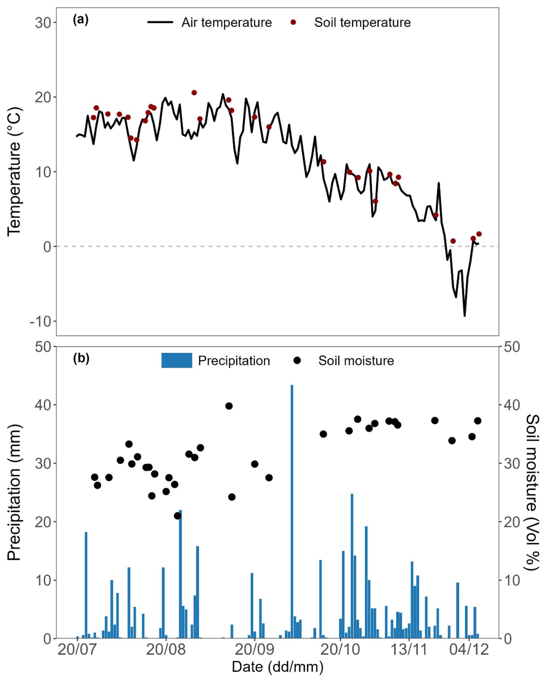
Figure 2 Seasonal variations in daily mean air (source Danish Meteorological Institute, 2025) and soil (5 cm) temperature (a) and daily precipitation (source Danish Meteorological Institute, 2025) and mean volumetric soil (0–5 cm) water content (b) over the entire observation period from July to December 2023.

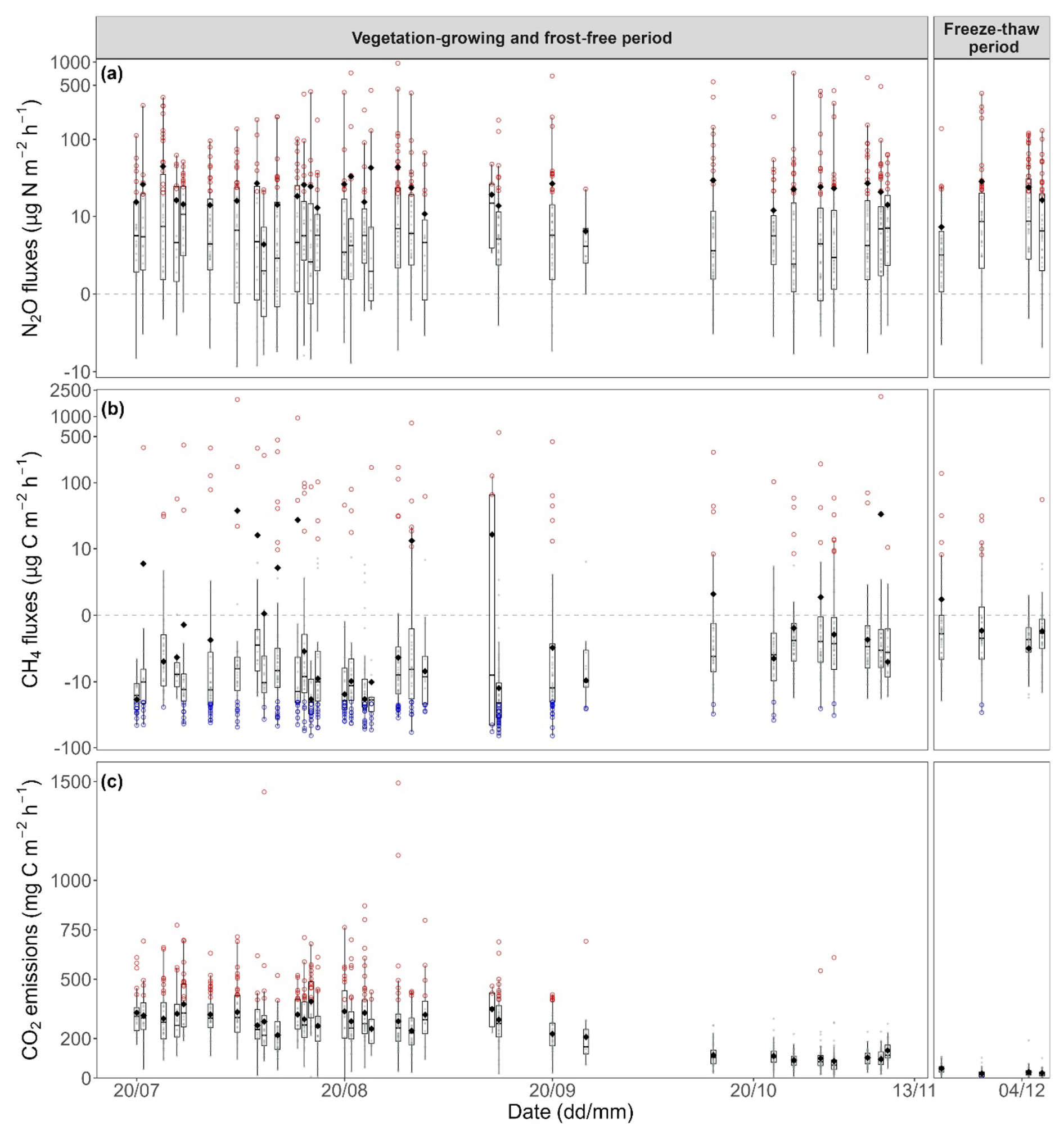
Figure 3 Fluxes of soil nitrous oxide (N₂O) (a), methane (CH₄) (b) and ecosystem (i.e. soil and plant) respiration (CO₂) (c) over the entire observation period from July to December 2023. The vegetation-growing and frost-free period spans from 20 July to 21 November 2023, while the freeze-thaw period spans from 22 November to 31 December 2023. In panels a-c, the black solid diamonds and lines inside the box represent the mean and median value, respectively. The box borders represent the 75th and 25th percentiles, and the whisker caps represent the 95th and 5th percentiles. The red and blue circle points represent hot spots and cold spots, respectively, and grey circle points represent neither hot spots nor cold spots of observation data. The definition of hot and cold spots can be found in the Materials and Methods section. To improve visualization across the wide range of flux values, the y-axes are displayed using a pseudo-logarithmic scale; this transformation was applied only to the y-axes for visual clarity and does not affect the original data values or statistical interpretation.

3.3 Spatial variability of N₂O, CH₄, and CO₂ fluxes

The cumulative N₂O fluxes over the vegetation-growing and frost-free period ranged from −0.01 to 9.96 kg N ha⁻¹ for all 56 sampling sites (Table S9). During the freeze-thaw period, the fluxes ranged from −0.01 to 0.74 kg N ha⁻¹. On average, the soils at our sampling sites acted as a significant net source of atmospheric N₂O, with a mean of 0.57 ± 0.20 kg N ha⁻¹. The CV between the different sampling sites was 259 %. The RF analysis showed that spatial variability in N₂O fluxes could be modeled with an overall performance of 87 % using the variables SOC, silt content, distance to the nearest tree, soil temperature and grass height (Table S10 and Fig. S4). The model displayed no probability of cold spots in the study areas and 54 % probability of hot spots (Table S10). Spatial variations in N₂O fluxes, as obtained through observations and predictions, showed a higher probability of hot spots close to the artificial ponds and a lower probability in the northeast section of the park (Figs. 4a and S5a).

Cumulative CH₄ fluxes over the vegetation-growing and frost-free period showed contrasted differences among the sampling sites (Table S9). That is, a sink of atmospheric CH₄ was observed at 45 out of 56 sampling sites, with cumulative CH₄ uptake ranging in magnitude from 0.04 to 0.83 kg C ha⁻¹. The remaining 11 sampling sites were net sources of atmospheric CH₄, with cumulative CH₄ emissions ranging from 0.01 to 5.44 kg C ha⁻¹. The CV between the different uptake sites was 60.5 % and the CV between the different source sites was 140.3 %, both were lower than the CV of 3154 % between all the sampling sites. By aggregating cumulative CH₄ and N₂O fluxes, the non-CO₂ GWP for all sampling sites ranged from −25.3 to 4272.8 kg CO₂eq ha⁻¹ (Table S9), with the spatial CV value 261 %. Based on the variables soil moisture, SOC, soil temperature, TN and distance to the nearest body of water, the RF model showed good predictive power for spatial variability of CH₄ fluxes, with the overall performance of 91 % (Fig. S4b and Table S10). Moreover, the model was more accurate in predicting cold spots of CH₄ uptake (78 %) than hot spots of CH₄ emissions (54 %) (Table S10). The spatial observations and predictions for our study areas showed a higher probability of hot spots closer to the artificial ponds and streams, particularly at two specific sites (Figs. 4b and S5b). However, the areas immediately adjacent to the water's edge were not necessarily identified as either hot spots or cold spots. Areas draining toward the artificial ponds showed the highest overall probability of becoming cold spots of CH₄ uptake over time, particularly in the northeastern and southern sections (Figs. 4c and S5c).

During the vegetation-growing and frost-free period, the cumulative ER-CO₂ emissions for the 56 sampling sites ranged from 0.7–10.2 Mg C ha⁻¹, with a mean of 5.48 ± 0.30 Mg C ha⁻¹. The CV between the different sampling sites was 40.3 %. Using the variables soil temperature, distance to the nearest body of water, soil moisture and clay content, the RF model achieved a 67 % performance for hot spot detection, but it did not show any cold spot probability (Fig. S4c and Table S10). Similar to the spatial variability of CH₄ emission hot spots, the frequency of observed high emissions and RF model showed a higher probability of ER-CO₂ emission hot spots closer to the artificial ponds and streams (Figs. 4d and S5d).

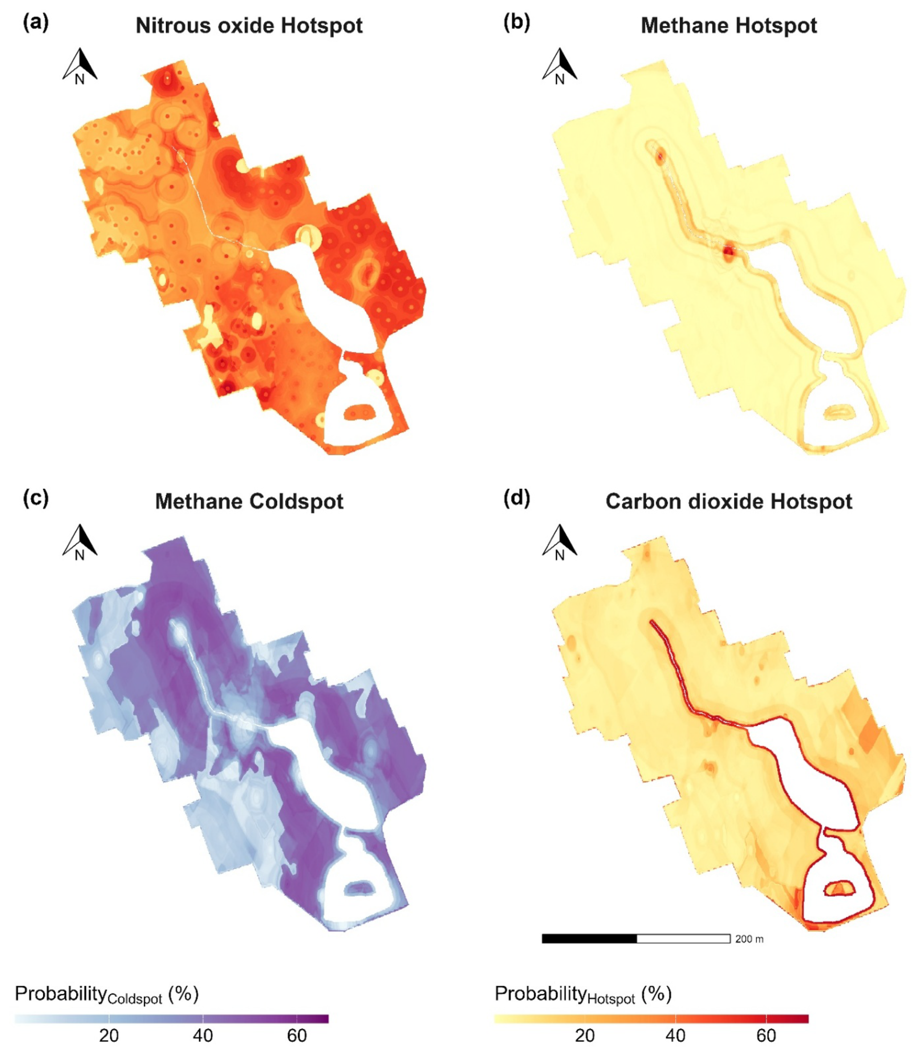
Figure 4 This map shows the area with the highest overall mean probability of being classified as nitrous oxide (N₂O) emission hot spots (a), methane (CH₄) emission hot spots (b), CH₄ uptake cold spots (c) and carbon dioxide (CO₂) emission hot spots (d). The definition of hot and cold spots can be found in the Materials and Methods section. In panel (a), the overlaid dots indicate the exact locations of the tree trunks.

3.4 Key factors driving the spatiotemporal variability

Although the simple regression analysis did not show a significant relationship between N₂O fluxes and environmental and soil variables, the RF model, which considers the interactions between the variables, could explain 80 % of the variance in N₂O fluxes (Fig. S4 and Table S10). Across the 56 sampling sites, the cumulative N₂O fluxes were also negatively correlated with soil pH (Fig. 5a).

To clearly show the key factors controlling the magnitude of CH₄ fluxes, we separated the observed data into CH₄ uptake rates and CH₄ emissions (both are expressed as positive values). Across the different uptake sites, the cumulative CH₄ uptake rates were negatively correlated with soil moisture, while positively correlated with the $\mathrm{C}/\mathrm{N}$ ratio (Fig. 5c and d). During the measurement period, the daily CH₄ uptake rates also showed a negative relationship with soil moisture (Fig. 6a). Across the different source sites, the cumulative CH₄ emissions were positively correlated with soil moisture (Fig. 5e), SOC (Fig. 5g) and TN (Fig. 5h), while negatively correlated with soil BD (Fig. 5f). A multiple regression analysis of all the CH₄ data showed that cumulative CH₄ fluxes were significantly controlled by the combined effect of soil moisture (SM), soil temperature (ST) and SOC (i.e., cumulative CH₄ fluxes = −5.77 + 0.10 SM + 0.17 ST + 0.01 SOC; r²=0.54, p<0.001).

Soil temperature showed significantly positive effects on both spatial and temporal variations of ER-CO₂ emissions (Figs. 5b and 6c). In addition, the daily ER-CO₂ emissions during the observation period were negatively correlated with soil moisture (Fig. 6b) and positively correlated with grass height (Fig. 6d).

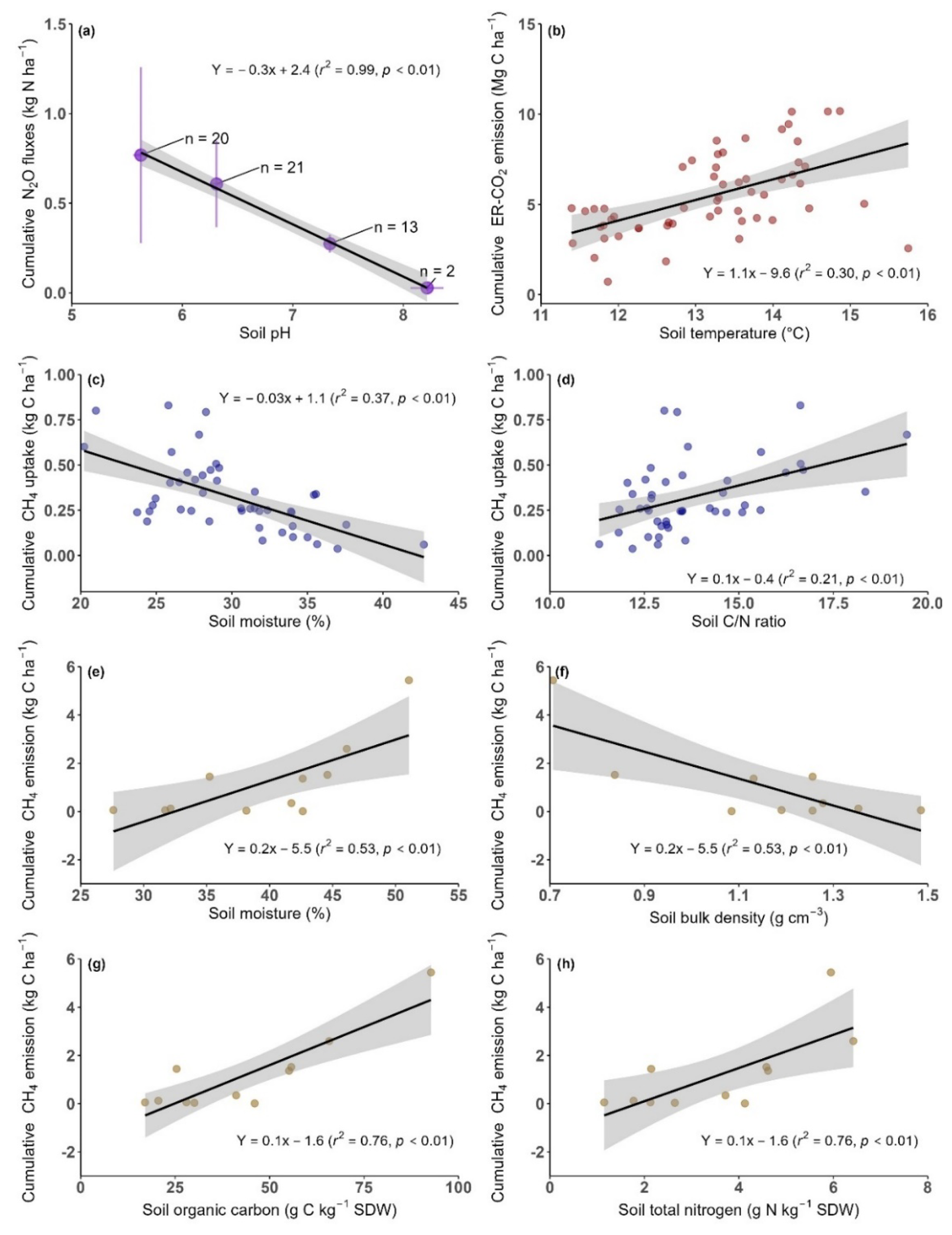
Figure 5 The relationships between cumulative nitrous oxide (N₂O) fluxes and soil pH (a), between cumulative ecosystem respiration (ER-CO₂) emissions and soil temperature (b), between cumulative methane (CH₄) uptake rates and soil moisture (c) and soil $\mathrm{C}/\mathrm{N}$ ratio (d), between cumulative CH₄ emissions and soil moisture (e), soil bulk density (f), soil organic carbon (g), and soil total nitrogen (h) across all the sampling sites. In panel a, soil pH was binned at a step width of 1 (i.e. 5.0–6.0, 6.0–7.0, 7.0–8.0 and >8.0), and points are given as mean values ± standard error, with numbers referring to the number of observations. SDW: soil dry weight. The shaded area of each panel represents the 95 % confidence band.

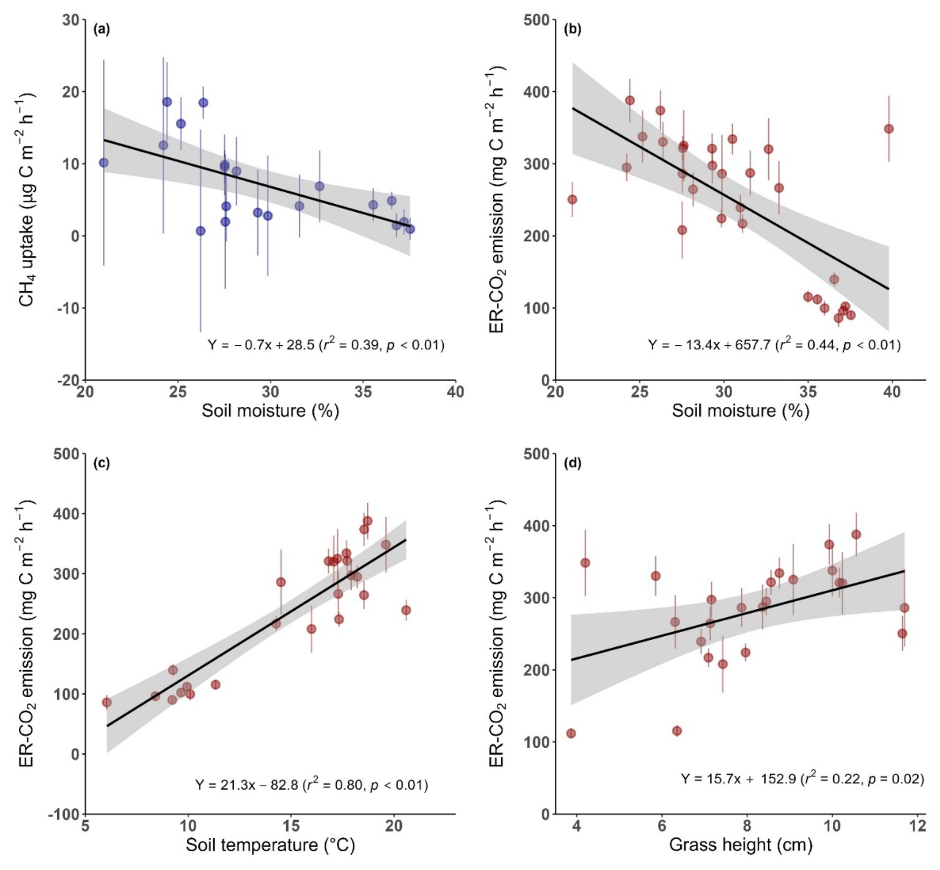
Figure 6 The relationships between methane (CH₄) uptake rates and soil moisture (a), between ecosystem respiration (ER-CO₂) emissions and soil moisture (b), soil temperature (c) and grass height (d) across the vegetation-growing and frost-free period. Points are given as mean values ± standard error across all the sampling sites at the same measurement time. The shaded area of each panel represents the 95 % confidence band.

4 Discussion

Urban green spaces play an important role in improving the quality of life and developing a sustainable urban environment (Giannico et al., 2021; Semeraro et al., 2021; Jabbar et al., 2022). However, many urban green spaces in both developed and developing countries are under-represented in global C and N cycling studies. As global urbanization continues to expand, this lack of representation contributes to high uncertainties in regional and national GHG budgets (Gao and O'Neill, 2020). In our study, we assessed soil GHG fluxes from an urban park in the Danish city of Aarhus during the vegetation-growing and frost-free period, as well as the freeze-thaw period. Our goal was to improve our understanding of the spatial and temporal patterns of these fluxes and to identify their key drivers. In addition, we aimed to demonstrate the necessity of addressing spatial variability in studies of GHG fluxes from urban green areas.

4.1 Temporal and spatial controls on soil N₂O fluxes in urban park environments

Over the entire observation period, the mean of all measurements resulted in an average daily N₂O emission of 23.8 µg N m⁻² h⁻¹ for the urban park. This value falls within the range (−1.1 to 84.5 µg N m⁻² h⁻¹) reported for urban green spaces in China, Singapore, Australia, Europe and North America (Maggiotto et al., 2000; Livesley et al., 2010; Davis et al., 2015; LeMonte et al., 2016; Braun and Bremer, 2018; Riches et al., 2020; Stefaner et al., 2021; Künnemann et al., 2023). However, our mean N₂O emissions in urban park environments are relatively higher than the reported ranges (0.5–23.4 µg N m⁻² h⁻¹) for natural grasslands and forests (Groffman et al., 2006, 2009; Groffman and Pouyat, 2009; Chen et al., 2014; Zhang et al., 2014; Ni and Groffman, 2018; Guo et al., 2022; Chen et al., 2023; Wang et al., 2025). These results corroborate previous findings that urbanization generally increases soil N₂O emissions compared to natural terrestrial ecosystems (Zhan et al., 2023). In this study, our observed N₂O emissions exhibit significant temporal and spatial variability, with CV values ranging from 45.6 % to 259 %. This high variability is consistent with patterns reported in other studies of forests, grasslands and agricultural systems (Kiese et al., 2003; Yao et al., 2009; van Delden et al., 2018; Wangari et al., 2022; Daelman et al., 2025). The highly dynamic nature of N₂O fluxes is primarily because soil N₂O fluxes are regulated by numerous abiotic and biotic factors that either fuel or restrain microbial processes (nitrification and denitrification) at various spatial and temporal scales (Butterbach-Bahl et al., 2013). For example, our regression analysis revealed a significant negative relationship between cumulative N₂O emissions and soil pH (Fig. 5a). The optimal pH range for denitrifiers is often reported to be 6.5–8.0 (Knowles, 1982; Šimek and Cooper, 2002). Thus, any increase above the mean soil pH observed in our study (pH 6.37) should theoretically increase N₂O production. However, at low soil pH levels, the reduction of N₂O to N₂ by N₂O reductase (nosZ) is substantially reduced, either due to the direct effect of pH on the assembly of N₂O reductase or due to shifts in the soil denitrification community toward denitrifiers lacking the nosZ gene (Čuhel et al., 2010; Xu et al., 2020). In other words, the partitioning of N₂O and N₂ during denitrification is affected by soil pH, with a higher proportion of N₂O present in acidic conditions. On the contrary, microbial activity may increase at higher pH values, leading to higher N₂O emissions. However, this may not be the case, as the N₂O yield during denitrification decreases with increasing pH (Čuhel et al., 2010).

For the sites we investigated, the high spatiotemporal variability in soil N₂O fluxes cannot be solely explained based on soil moisture status and/or temperature changes. Nevertheless, distinct “hot moments” of soil N₂O emissions were observed during the freeze-thaw period. These observations suggest that soil N₂O fluxes are sensitive to short-term changes in environmental factors, such as soil temperature changes, during the freeze-thaw period. Other studies have reported similar pulses of N₂O fluxes during freeze-thaw periods in boreal and temperate ecosystems, including forests, grasslands and agricultural fields (Butterbach-Bahl et al., 2002; Luo et al., 2013; Wagner-Riddle et al., 2017). However, our observation of this phenomenon in urban green spaces is novel. Pulses of N₂O emissions during freeze-thaw periods are generally attributed to the close coupling of microbial mineralization, nitrification, and denitrification, occurring under conditions in which the surface soil is close to moisture saturation, and increased availability of easily degradable C and N substrates. This can be due to the death of soil microbes from frost, as suggested by De Bruijn et al. (2009).

Although our linear regression analysis did not reveal a significant relationship between soil temperature and N₂O fluxes, the RF model identified soil temperature as one of the most influential predictors (Fig. S4). Nevertheless, the RF model showed that total N content is not one of the key predictors of N₂O fluxes, while SOC is a significant predictor. SOC has been considered as a major constituent of soil organic matter (SOM). Higher SOM levels provide more essential macro- and micro-nutrients, improving microbial activities and associated N₂O production (Butterbach-Bahl et al., 2013). Despite the limited ability of the RF model to accurately classify N₂O emission hot spots (Fig. 4a), the spatial probability maps indicate that large portions of the park show a moderate likelihood (39 ± 13 %) of becoming hot spots under specific conditions. This implies that hot spots are not confined to fixed locations but instead emerge dynamically in response to transient environmental triggers, such as freeze-thaw events or soil saturation. To improve hot spot prediction, we emphasize the need for higher-frequency flux measurements, particularly during periods of rapid environmental change and finer resolution of soil data (Helfenstein et al., 2024).

4.2 Spatiotemporal patterns and environmental controls of CH₄ fluxes from urban park soils

During the observation period, the soils in the urban park were predominantly a weak sink for atmospheric CH₄ (−0.26 µg C m⁻² h⁻¹ on average over all measurements), though they sporadically changed from a sink to a source after rainfall events. This sink-to-source dynamic, driven by soil water status, is consistent with observations from an urban lawn in Australia (van Delden et al., 2018). Moreover, the magnitude of the mean CH₄ fluxes observed in our study was at the lower end of the reported uptake rates from urban green spaces in other European countries and the USA (Groffman and Pouyat, 2009; Bezyk et al., 2022; Trémeau et al., 2024). In contrast, previous studies have reported that soil CH₄ fluxes in natural forests and grasslands ranged from −3.9 to −168.7 µg C m⁻² h⁻¹ (Goldman et al., 1995; Groffman et al., 2009; Groffman and Pouyat, 2009; Czóbel et al., 2010; Chen et al., 2014; Zhang et al., 2014; Ni and Groffman, 2018; Chen et al., 2023; Wang et al., 2025). These findings suggest that urbanization generally reduces soil CH₄ uptake compared to natural terrestrial ecosystems (Zhan et al., 2023).

Regression analysis revealed a strong negative correlation between CH₄ uptake rates and soil moisture. However, no significant relationship was observed between CH₄ uptake rates and soil temperature. These results suggest that soil moisture is the dominant environmental driver of the temporal variability of CH₄ fluxes compared to temperature in this urban park. Similar results have been observed in many studies of urban green spaces or natural forests and grasslands (van Delden et al., 2018; Liu et al., 2019). Generally, soil moisture affects both soil gas diffusion and the microbial populations that regulate the CH₄ dynamics (Potter et al., 1996; Smith et al., 2018; Bezyk et al., 2023). At high soil moisture contents, CH₄ uptake is usually limited by reduced diffusivity into the soil. Accordingly, these results suggest that future studies require high-temporal-resolution soil hydrological observations to better trace the dynamics of CH₄ fluxes.

In this study, cumulative CH₄ fluxes for all 56 sampling sites were used to analyze the spatial variability (Table S9). The results showed pronounced differences in cumulative CH₄ fluxes among the sampling sites, i.e., CH₄ emissions occurred in 11 of the 56 sites. These significant CH₄ emissions are likely due to the predominance of soil water saturation and the accumulation of C substrates in topsoils, as sites functioning as net sources of CH₄ to the atmosphere were positioned closer to artificial ponds and streams within the urban park. Our regression analysis revealed that soil moisture was positively correlated with cumulative CH₄ emissions, while negatively correlated with cumulative CH₄ uptake (Fig. 5c and e). The opposite response of cumulative CH₄ fluxes to soil moisture status between source and sink sites is likely due to the fact that higher soil moisture contents suppress gas diffusion and increase the volume of anaerobic soil. This dual effect suppresses methanotrophy and stimulates methanogenesis, thereby reducing CH₄ oxidation and promoting CH₄ production (McLain and Ahmann, 2008; Praeg et al., 2014). Moreover, the cumulative CH₄ emissions increased with increasing SOC and TN. This corroborates previous findings that SOC and TN are important factors in controlling ecosystem CH₄ emissions because they can provide C and N substrates to methanogens, and thus, enhancing their activities and associated CH₄ production (Ma et al., 2020; Zhao and Zhuang, 2024). We further observed that the studied sites with higher SOC values typically exhibited relatively low BD values. This inverse relationship could explain why cumulative CH₄ emissions decreased as BD increased in our study (Fig. 5f). Additionally, the cumulative CH₄ uptake was strongly and positively correlated with soil $\mathrm{C}/\mathrm{N}$ ratios. Lower $\mathrm{C}/\mathrm{N}$ ratios in urban soils likely support higher rates of N transformation, particularly mineralization and nitrification. However, increased soil N availability can inhibit methanotrophic activities and associated CH₄ oxidation (Steinkamp et al., 2001; Zhan et al., 2023). Considering all 56 sampling sites together, the spatial variability of CH₄ fluxes was significantly regulated by the combined effects of soil moisture, temperature and SOC. Furthermore, these three variables were also included in the RF model to predict CH₄ hot and cold spots. Previous studies have similarly reported that soil moisture, temperature and C availability are the main drivers shaping the spatial patterns of CH₄ fluxes across heterogeneous landscapes (West et al., 1999; Olefeldt et al., 2013; Kaiser et al., 2018; Yu et al., 2019).

4.3 Controls of ecosystem respiration (CO₂) emissions in urban park environments

In this study, the average ER-CO₂ emissions were 228 mg C m⁻² h⁻¹ when using the arithmetic mean of all measurements. Our observed ER-CO₂ emissions are consistent with the reported range (142–298 mg C m⁻² h⁻¹) for open lawns, treed lawns, and urban woodlands in France (Künnemann et al., 2023), but higher than the emissions recorded in urban woodlands (54–100 mg C m⁻² h⁻¹) by Groffman et al. (2009) and Chen et al. (2013) and natural grasslands (65–82 mg C m⁻² h⁻¹) by Wang et al. (2025). Over the entire observation period, the variability in ER-CO₂ emission was negatively correlated with soil moisture and positively correlated with soil temperature and grass height (Fig. 6b–d). Ecosystem respiration depends heavily on plant respiration and microbial decomposition. Grass height is a proxy for aboveground biomass and, consequently, exerts a positive effect on ER-CO₂ emissions. This positive correlation with aboveground biomass has been well documented in previous studies (Ding et al., 2007; Yao et al., 2013). High levels of soil moisture can restrict the availability of O₂ within the soil matrix, thereby creating conditions conducive to anoxic processes, and resulting in reduced CO₂ emissions (Hao et al., 2025). Moreover, the SOC decomposition process is constrained by anoxia, which restricts the release of nutrients necessary for CO₂ formation (Keiluweit et al., 2017). This interpretation was indirectly supported by our observations that cumulative CH₄ fluxes were positively correlated with soil water-filled pore space (WFPS) across all sampling sites (Fig. S6). This positive relationship indicates that the anoxia under high soil moisture conditions stimulates CH₄ emissions, while inhibiting aerobic CH₄ uptake and CO₂ emissions. Nevertheless, increases in soil temperature can alleviate limitations on plant function and the microbial decomposition of SOC. This promotes plant biomass accumulation, autotrophic and heterotrophic respiration and, thus, ecosystem respiration (i.e., ER-CO₂ emissions).

Across all the 56 sampling sites, our results showed that soil temperature was the dominant factor influencing the spatial variability in cumulative ER-CO₂ emissions, with a particularly strong effect in sites around artificial ponds. Furthermore, the RF model confirmed this pattern of CO₂ emissions across the landscape. That is, ER-CO₂ hot spots were concentrated around artificial ponds where grass heights were higher. As previously mentioned, elevated soil temperatures stimulate greater ER-CO₂ emissions by promoting vegetation growth under unlimited soil water conditions. These results suggest that future work should focus on integrating biomass estimates from remote sensing (Hoyos-Santillan et al., 2025). This could serve as an alternative to grass-height measurements, which are currently limited to sampling sites. In other words, integrating remote sensing of vegetation dynamics with gas flux monitoring could provide a scalable method of linking plant phenology with ER-CO₂ emission variability in urban green spaces.

4.4 Implications for future studies in urban green spaces

In this study, we view the RF model as a complement, rather than a replacement for empirical methods. For example, in this study, the RF model helped identify the combined effects of multiple factors, such as SOC for N₂O, soil temperature for CH₄ and clay content for CO₂, which were not always significant in empirical regressions. Combining these two approaches is especially valuable in the context of urban GHG flux budgets, where spatial heterogeneity and temporal variability complicate the process of upscaling and extrapolating from limited site measurements. This integration allows for more precise evaluations of the contribution of urban green spaces to city-scale GHG fluxes.

Practically speaking, city managers and policymakers could use these predictive frameworks to identify “hotspot-prone” zones in urban parks. They could then direct targeted interventions to these zones rather than treating green spaces as homogeneous units. This approach may increase the efficiency of climate mitigation actions by allocating management resources to areas where emissions are likely to be most intense. Beyond Aarhus, this framework could be adopted by other cities with similar green space structures, making it a relevant tool for integrating soil GHG fluxes into urban carbon accounting.

5 Conclusions

Despite the rapid urban sprawl occurring around the world, urban green spaces and their biogeochemical carbon and nitrogen cycles are still generally understudied. The limited urban soil GHG flux data available does not accurately reflect spatial and temporal variations in fluxes, resulting in GHG budgets with large uncertainties. This study provides insights into the spatiotemporal variability of soil CH₄ and N₂O fluxes and ecosystem CO₂ emissions in an urban park located in a hilly landscape, based on measurements of the vegetation-growing and frost-free period as well as the freeze-thaw period across the 56 sites that vary in vegetation type and landscape position. On average, our results show that the soils in urban green spaces primarily function as a source of N₂O and a weak sink of CH₄. Moreover, our observations confirm significant temporal and spatial variations in soil CH₄ and N₂O fluxes and ecosystem CO₂ emissions. This high variability is strongly related to changes in environmental and landscape parameters such as vegetation structure, soil hydrothermal conditions, pH and the availability of carbon and nitrogen. These findings underscore the necessity of additional measurement campaigns in urban green spaces. These campaigns should have an experimental design that allows for large spatial coverage and a high temporal sampling frequency when determining soil fluxes. Based on our comprehensive observed datasets, however, we developed RF models to predict the probability of GHG hot spots and/or cold spots. While model performance varied depending on trace gas and driver complexity, the RF approach effectively captured the spatial heterogeneity and provided a scalable framework for mapping GHG fluxes across urban green spaces. Overall, our findings may allow for better scaling of GHG fluxes in urban green spaces and enable a more accurate assessment of how urbanization changes landscape fluxes.