Sphagnum and herbaceous net ecosystem exchanges in a Pyrenean peatland: a long-term study using the ISBA model

Peatlands play a crucial role in the global carbon cycle, acting as long-term carbon sinks. However, their stability is increasingly threatened by climate change, particularly through rising temperatures and the intensification of droughts. This study focuses on the Bernadouze peatland in the Pyrenees Mountains and aims to validate a newly implemented Sphagnum Plant Functional Type (PFT) in the ISBA land surface model, assess the temporal evolution of carbon fluxes over the past 64 years, and investigate the factors influencing carbon accumulation, with a particular emphasis on drought events.

The model was validated using in situ data, demonstrating reasonable carbon flux estimations. Using this validated model, we reconstructed the net ecosystem exchange (NEE) dynamics of the Bernadouze peatland from 1959 to 2022. The results reveal significant interannual variability in NEE, largely driven by air temperature and water table depth. While the peatland has remained a carbon sink, extreme droughts such as those in 1989, 1994, 2003, and most recently 2022 have led to substantial CO₂ emissions.

Our findings suggest that although increasing temperatures have extended the growing season and enhanced gross primary productivity (GPP), the rising frequency and intensity of droughts pose a long-term risk to peatland carbon storage. The dryness index developed in this study appears to be a strong predictor of summer and annual NEE, offering a potential tool for estimating carbon fluxes in peatlands lacking direct measurements.

1 Introduction

Peatlands are vital to the global carbon cycle, serving as significant carbon reservoirs and actively exchanging CO₂ and methane with the atmosphere (Gorham et al., 2012). However, the stability of these carbon stocks is increasingly threatened by global warming (Page and Baird, 2016; Carter et al., 2012; Loisel et al., 2021), highlighting the need for precise models to predict their carbon balance. This concern is particularly relevant in mountainous regions, where climate change is expected to be more pronounced (Rogora et al., 2018), potentially affecting the functioning of mountain peatland ecosystems.

Models have been developed to represent the biophysical and biogeochemical processes that occur in peatlands. Sphagnum mosses are considered the dominant vegetation in Northern peatlands (Turetsky, 2003) and function differently from vascular plants, lacking stomata to regulate their water content (Clymo and Hayward, 1982). They acquire water either by absorbing atmospheric precipitation or through capillary action directly from the soil surface. Their presence is also crucial for the accumulation of organic carbon in peatlands, as they have a lower litter decomposition rate compared to vascular plants (Scheffer et al., 2001; Lang et al., 2009). As a result, various classes of models have been developed to account for the role of Sphagnum mosses, reflecting diverse approaches. Dynamic vegetation and ecosystem models, developed as offline tools without atmospheric, climate, or carbon feedbacks, have since incorporated these processes into their frameworks (Wania et al., 2009; Frolking et al., 2010; Walker et al., 2017; Gong et al., 2020; Metzger et al., 2016). Furthermore, specific Continental Surface Models (CSMs) have been developed for the representation of peatlands (St-Hilaire et al., 2010; Wu and Blodau, 2013; Wu et al., 2016; Wania et al., 2013; Park et al., 2018). There have also been ongoing efforts to improve the representation of Sphagnum mosses in Global Land Surface models, with varying degrees of complexity and scope (Chadburn et al., 2015; Porada et al., 2016; Druel et al., 2017; Qiu et al., 2019; Shi et al., 2015; Grant et al., 2012; Shi et al., 2021).

Efforts to study peatland responses to drought episodes increasingly rely on field measurements and mesocosm experiments (Sterk et al., 2023; Robroek et al., 2024), though research in this area remains limited. A significant limitation of these methods is the scarcity of continuous field measurements capturing medium-term carbon fluxes over decades or longer. Such data would offer critical insights into the frequency and long-term effects of episodic drought events on carbon accumulation. Current carbon flux measurements are generally restricted to contemporary dynamics, which exhibit notable interannual variability, complicating efforts to extrapolate trends over medium or long-term timescales (Young et al., 2021). To explore long-term carbon accumulation dynamics, peat coring analyses provide a reliable means of determining the average LOng-term apparent Rates of C Accumulation (LORCA), offering insights into millennia of accumulation (Turunen, 2003). Additionally, based on the same methodology, the Actual Rate of Carbon Accumulation (ARCA) can be determined, theoretically enabling the observation of carbon accumulation over decades or centuries (Chaudhary et al., 2017). Interest in ARCA has grown recently, particularly as a means of assessing the effects of climate and environmental changes on carbon accumulation. However, its reliability has been questioned (Young et al., 2021; Frolking et al., 2014), as ARCA does not accurately reflect the net balance of organic carbon in peatlands. An alternative approach involves modeling exercises that combine peat core age data with empirical models of organic matter decomposition. This allows reconstruction of historical carbon fluxes, linking absorbed and released carbon to initial peatland carbon stock (Yu, 2011; Packalen and Finkelstein, 2014; Frolking et al., 2010; Bunsen and Loisel, 2020; Loisel and Yu, 2013). In this study, we propose another complementary approach, leveraging a CSM that use atmospheric forcing data as input. Observationally-based atmospheric forcings, available with hourly resolution for some regions since the 1960s, provide a robust basis for modeling peatland evolution over the past several decades. Against the backdrop of Europe's severe drought in 2022 (Faranda et al., 2023), recent research on the Bernadouze peatland in the Pyrenees mountains identified a significant carbon release to the atmosphere during this event, supported by six years of field data (Garisoain et al., 2024). This drought presents a compelling case within a 64 year record, raising questions about its severity as an isolated event versus its representation of a broader trend. Additionally, it prompts examination of whether the peatland's functioning during 2022 aligns with long-term behavior.

To address these questions, this study pursues three key objectives: (1) Implementation and first-site evaluation of a new Sphagnum Plant Functional Type (PFT) within the ISBA land surface model; (2) Assessment of the temporal evolution of carbon fluxes from the Bernadouze peatland over the past 64 years; (3) Investigation of the factors influencing carbon accumulation, with a particular focus on drought episodes.

2 Materials and methods

2.1 Study site

The Bernadouze peatland, located at an altitude of 1343 m in the eastern French Pyrenees (42.80273° N; 1.42361° E), covers roughly 4.7 ha and is part of a national biological reserve. Designated as a regional biological reserve since 1983 and a Natura 2000 site since 2007, it is one of the four sites of the French National Peatland Observatory Service SNO-Tourbieres. Characteristic of alpine and southwestern European mountainous peatlands, it is classified as a soligenous fen, continuously receiving water from precipitation and surface runoff. It has formed over the past 5000 years within a 1.4 km watershed with steep slopes averaging 50 %. A beech forest surrounds the fen, extending up to 1800 m. The peatland has an average peat depth of 2 m, reaching up to 6 m in some areas. The vegetation comprises species typical of both ombrotrophic areas, such as Sphagnum palustre and Sphagnum capillifolium, and minerotrophic areas, including Carex demissa and Equisetum fluviatile (Henry et al., 2014). This distribution is illustrated in Fig. 1 of Garisoain et al. (2023), which shows the spatial arrangement of vegetation types across the study site.

2.2 Environmental monitoring

Piezometer wells are 50 mm diameter PVC tubes, distributed across the peatland to cover the full spatial extent of the site (Fig. 1 from Garisoain et al., 2024), and their placement corresponds to the locations where chamber measurements were conducted. Water table depth (WTD) data were recorded at 1 h intervals, and the mean value from the nine piezometers is used throughout the study. As in precedent studies of the same peatland (Garisoain et al., 2023, 2024) we used the S2M reanalysis, which combines the French weather service SAFRAN meteorological reanalysis (8 km resolution) with the SURFEX/ISBA-Crocus snow cover model (Vernay et al., 2022). The S2M chain was applied in a local mode at the scale of the “Couserans” massif (a mountainous region in the central Pyrenees, southwestern France), assuming homogeneous weather conditions across the massif for equivalent altitudes but accounting for local topographic features in the calculation of shortwave radiation. The S2M model has a vertical resolution of 300 m and provides hourly outputs. The topographical features of the peatland, including altitude, slope, and aspect, were carefully accounted for to ensure that the atmospheric variables extracted for the site accurately represent local conditions.

2.3 Carbon fluxes

Hourly validated time series of CO₂ fluxes (GPP, ER, and NEE) spanning 2017 to 2022 are available, as detailed by Garisoain et al. (2024). These time series were derived from statistical models based on monthly CO₂ flux measurements using the static chamber technique. The use of the statistical model allows reconstruction of daily fluxes, enabling direct comparison with the ISBA model outputs at the same temporal resolution. The reconstructed fluxes are considered spatially representative of the peatland due to the coverage and replication of the chamber measurements. In the following sections, these reconstructed datasets are used as a reference for model validation, and readers should note that the validation is performed against the derived statistical model rather than the raw measurements.

2.4 Model development

In the present study, we utilize the ISBA model, which is part of the SURFEX land surface modeling platform (Version 9) and serves as the land surface component of the global Earth System Model CNRM-ESM (Delire et al., 2020). ISBA is widely employed to simulate surface processes, but it does not currently represent mosses or Sphagnum, which are essential components of ecosystems such as peatlands. To address this limitation, we introduce a new plant functional type (PFT) designed specifically for modeling mosses and Sphagnum within the ISBA framework. This work details the implementation of this novel PFT and the associated modifications to the model to better represent the dynamics of peatland ecosystems. The other PFTs, representing vegetation types such as herbaceous plants and trees, have been thoroughly described in the existing literature (Gibelin et al., 2008).

2.4.1 Photosynthesis of Sphagnum

Plant photosynthesis is modeled according to the description by Goudriaan (1986) and Jacobs (1994), focusing on the equations involving the dependence on mesophyll conductance or CO₂ (Eq. 1) and light dependency (Eq. 2).

$$\begin{array}{}\text{(1)}& \text{Am}={\text{Am}}_{\max }\times (\mathrm{1}-e^{\frac{-{\text{gm}}^{*}(C_i-\mathrm{\Gamma })}{{\text{Am}}_{\max }}})\end{array}$$

Am is the assimilation rate under light-saturated conditions ($\mathrm{kg}{\mathrm{m}}^{-\mathrm{2}}{\mathrm{s}}^{-\mathrm{1}}$), Am_max is the maximum assimilation rate ($\mathrm{kg}{\mathrm{m}}^{-\mathrm{2}}{\mathrm{s}}^{-\mathrm{1}}$), gm^* is the mesophyll conductance without water stress (m s⁻¹), C_i (kg m⁻³) is the internal mesophyll CO₂ concentration (see Eq. 4) and Γ (kg m⁻³) is the CO₂ compensation point, meaning the CO₂ concentration below which the plant no longer fixes CO₂.

$$\begin{array}{}\text{(2)}& A_{\mathrm{n}}=(\text{Am}+R_{\mathrm{d}})\times (\mathrm{1}-e^{\frac{-\mathit{ϵ}{I}_{\mathrm{a}}}{\text{Am}+R_{\mathrm{d}}}})-R_{\mathrm{d}}\end{array}$$

A_n is the net assimilation rate $\mathrm{kg}{\mathrm{m}}^{-\mathrm{2}}{\mathrm{s}}^{-\mathrm{1}}$, R_d is the “dark respiration” $\mathrm{kg}{\mathrm{m}}^{-\mathrm{2}}{\mathrm{s}}^{-\mathrm{1}}$, ϵ the light use efficiency kg J⁻¹ and I_a is the photosynthetically active radiation W m⁻².

$$\begin{array}{}\text{(3)}& R_{\mathrm{d}}={\displaystyle \frac{\text{Am}}{\mathrm{9}}}\end{array}$$

R_d is the mitochondrial respiration, empirically fixed.

In ISBA, gm^* and Am_max depend on the PFT parameters and the leaf surface temperature following a Q₁₀ function, modified by Collatz et al. (1992) to account for inhibitions (Jacobs et al., 1996). Then, gm^* is replaced by gm, which allows accounting for plant water stress conditions (see Table A1). Thus, the effect of stomatal closure on photosynthesis in ISBA is controlled by gm, not by gs (the stomatal conductance), which is calculated as a function of A_n and used solely to determine transpiration fluxes (see Eq. B5, Appendix B).

To model the photosynthesis of Sphagnum mosses, only mesophyll conductance has been considered to contribute to photosynthesis, even though the transfer of CO₂ within the hyaline cells is still poorly understood (Weston et al., 2015). Since Sphagnum mosses lack stomata, stomatal conductance is no longer defined for the Sphagnum PFT. Therefore, the relationship between Sphagnum moss photosynthesis and Sphagnum moss water content is accounted for through gm. Shi et al. (2021) and Walker et al. (2017) described Sphagnum moss photosynthesis using the concept of total Sphagnum moss CO₂ conductance, derived from measurements by Williams and Flanagan (1998) relating Sphagnum moss water content to Sphagnum moss CO₂ conductance. In our case, we relate Sphagnum moss mesophyll conductance and total Sphagnum moss CO₂ conductance. Although they are not the same physical quantity. In Jacobs (1994) description, gm is the closest approximation to total CO₂ conductance. Hence, the normalized total Sphagnum moss CO₂ conductance (g_tot) was first defined following Gong et al. (2020) (Eq. 4 and Fig. A1). This variable was then used to parameterize the relationship between gm and g_tot proposed by Williams and Flanagan (1998) (Eq. 5).

$$\begin{array}{}\text{(4)}& {\displaystyle }{g}_{\mathrm{tot}}=\left\{\begin{array}{cl}(\mathit{\beta }+\mathit{\gamma }\times w_{\mathrm{Sp}}+\mathit{\eta }\times w_{\mathrm{Sp}}^{\mathrm{2}})& \text{ if }{w}_{\mathrm{opt}}\ge w_{\mathrm{Sp}}\ge w_{\min }\\ (\mathrm{1}-\mathrm{0.8}\times \frac{w_{\mathrm{Sp}}-w_{\mathrm{opt}}}{w_{\max }-w_{\mathrm{opt}}})& \text{ if }{w}_{\mathrm{Sp}}\ge w_{\mathrm{opt}}\\ \mathrm{0}& \text{ if }{w}_{\mathrm{Sp}}\le w_{\min }\end{array}\right.\text{(5)}& {\displaystyle }\text{gm}=\mathit{\alpha }\times g_{\mathrm{tot}}\text{(6)}& {\displaystyle }\mathit{\eta }={\displaystyle \frac{\mathit{\beta }-\mathrm{1}}{w_{\mathrm{opt}}^{\mathrm{2}}}}\text{(7)}& {\displaystyle }\mathit{\gamma }=-\mathrm{2}\times w_{\mathrm{opt}}\times \mathit{\eta }\end{array}$$

Where w_Sp is the water content of Sphagnum mosses (g g⁻¹), g_tot is the normalized total conductance, β, γ, η are coefficients given in Table A2, w_min and w_max respectively the maximum and minimum water content of Sphagnum mosses (g g⁻¹), w_opt (g g⁻¹) is the water content of Sphagnum that maximizes g_tot and α (m s⁻¹) is a parametrized coefficient given in Table A2.

2.4.2 Leaf area index – Canopy scaling

The evolution of Sphagnum moss biomass results from the balance between carbon assimilation through photosynthesis and Sphagnum moss mortality, calculated according to Eq. (8):

$$\begin{array}{}\text{(8)}& {\displaystyle \frac{\mathrm{\Delta }B}{\mathrm{\Delta }t}}=A_{\mathrm{c}}-R_{\mathrm{c}}-{\displaystyle \frac{B}{\mathrm{\Delta }t}}\exp \left({\displaystyle \frac{-t}{\mathit{\tau }}}\right)\end{array}$$

where B is the active biomass of Sphagnum mosses in kg m⁻², $\frac{B}{\mathrm{\Delta }t}\exp \left(\frac{-t}{\mathit{\tau }}\right)$ is the mortality of the Sphagnum moss biomass, τ is the characteristic mortality time, Δt is a timestep of 1 d, A_c is the net assimilation of the Sphagnum mosses canopy and R_c is the respiration of Sphagnum mosses canopy ($A_{\mathrm{c}}=\text{LAI}\times A_{\mathrm{n}}$, $R_{\mathrm{c}}=\text{LAI}\times R_{\mathrm{d}}$).

The LAI is directly calculated from the leaf biomass reservoir B according to:

$$\begin{array}{}\text{(9)}& \text{LAI}=B\times \text{SLA}\end{array}$$

where SLA (specific leaf area) is a foliar vegetation index representing the leaf area per unit of assimilated carbon (${\mathrm{m}}^{\mathrm{2}}{\mathrm{m}}^{-\mathrm{2}}{\mathrm{kg}}^{-\mathrm{1}}$).

$$\begin{array}{}\text{(10)}& \text{SLA}=e\times N_{\mathrm{m}}+f\end{array}$$

Here, N_m is the mass-based nitrogen concentration in the leaf (Calvet and Soussana, 2001). The SLA is defined for each vegetation type.

Once net assimilation is calculated, multiplying by the LAI allows for scaling from the individual Sphagnum strand to the Sphagnum canopy. The ISBA model follows the assumption of maintaining constant temperature, humidity, and CO₂ concentration throughout the canopy. Additionally, a radiative transfer model for photosynthetically active radiation was developed by Carrer et al. (2013), allowing for the representation of light diffusion within a canopy based on its LAI. This module accounts for the decrease in light radiation along the vertical profile of the canopy (with more light at the top of the canopy) as well as the diffusion of light towards the lower parts of the canopy. The attenuation of light within the canopy thus leads to a decreasing vertical profile of photosynthesis within the canopy. Leaf respiration, on the other hand, is assumed to be constant along the vertical profile of the canopy. Canopy respiration corresponds to the respiration calculated at the leaf level multiplied by the LAI.

2.4.3 Biomass pools

In the original ISBA model, vegetation is represented by up to six biomass reservoirs: leaves, stem, wood, fine and coarse roots, and a small storage pool corresponding to nonstructural carbohydrates (Gibelin et al., 2008; Delire et al., 2020). For grass/herbaceous PFTs', wood and coarse roots are excluded. Leaf biomass evolves based on photosynthetic carbon assimilation and is reduced by turnover, respiration, and allocation to other pools. Leaf area index (LAI) is derived from leaf biomass and specific leaf area, which depends on both PFT and nitrogen content. Mortality and turnover are PFT-dependent and climate-sensitive, especially for leaves. Photosynthesis and respiration are computed at sub-daily time steps, while the biomass pools evolve on a daily basis.

For Sphagnum, the structure was simplified to reflect its particular growth strategy and morphology. Only two biomass reservoirs are considered: B, representing the photosynthetically active green biomass, and B_brown, the dead biomass. The latter is fed by senescence from the green biomass and follows a similar formulation to the original model's decay processes, with an adjusted decay rate specific to Sphagnum. This minimalist representation captures the essential dynamics of Sphagnum growth and decomposition, consistent with its role in peat accumulation and its lack of differentiated organs like leaves or roots.

The brown Sphagnum mosses (B_brown) are uniformly distributed over 10 cm of the soil profile, and this vertical distribution is maintained throughout the simulation.

2.4.4 Sphagnum water content

To model the evolution of the water content in Sphagnum mosses, we followed the work of St-Hilaire et al. (2010), considering a linear relationship between the soil water content at 10 cm and the water content of Sphagnum mosses.

$$\begin{array}{}\text{(11)}& w_{\mathrm{Sp}}=b\times w_{\mathrm{soil},\mathrm{10}\mathrm{cm}}+c\end{array}$$

where w_Sp is the water content of Sphagnum mosses in g g⁻¹ and w_soil,10 cm is the soil water content at 10 cm in m³ m⁻³. The empirical coefficients b and c are given in Table A2.

The precipitation interception reservoir is considered negligible. Consequently, Sphagnum mosses receive water primarily through capillary action from the soil within 10 cm of the surface. Although direct interception of rainfall also contributes in reality, this process is not explicitly modeled here. Instead, we account only for the effect of capillarity by relating the water content of Sphagnum to that of the upper 10 cm of soil. Precipitation that would otherwise be intercepted bypasses the moss canopy and infiltrates directly into the soil, thereby influencing both soil and Sphagnum water content.

2.4.5 Sphagnum evaporation

Given that Sphagnum mosses do not possess stomata, we consider that the latent heat flux from the vegetation is solely due to the evaporation of water from the their epidermal cells. The plant transpiration phenomenon controlled by stomata is therefore eliminated here. Thus, we have:

$$\begin{array}{}\text{(12)}& \begin{array}{rl}& E_{\mathrm{veg}}={\displaystyle \frac{F_{\mathrm{veg}}}{R_{\mathrm{a}}+R_{\mathrm{sp}}}}\times \left(q_{\mathrm{sat}}\right(T_{\mathrm{s}})-q_{\mathrm{a}})\times {\mathit{\rho }}_{\mathrm{a}}\\ & \text{with }{R}_{\mathrm{a}}={\displaystyle \frac{\mathrm{1}}{C_H{V}_{\mathrm{a}}}}\end{array}\end{array}$$

E_veg is the latent heat flux from the vegetation (see Eq. B5, Appendix B) in $\mathrm{kg}{\mathrm{m}}^{-\mathrm{2}}{\mathrm{s}}^{-\mathrm{1}}$. R_a and R_sp represent the air and Sphagnum canopy resistances, respectively. F_veg is the fraction of vegetation, q_sat(T_s) is the specific humidity at saturation at temperature T_s, T_s is the surface temperature and q_a is the specific humidity of the air at reference altitude z_a. ρ_a is the air density at altitude z_a, C_H is the drag coefficient, and V_a is the wind speed at z_a.

R_sp has been modeled following the work of Bond-Lamberty et al. (2011) and Gong et al. (2020), who experimentally established a relationship between the resistance of the Sphagnum canopy and the water content of the Sphagnum mosses. The Sphagnum moss resistance to water decreases towards low values when the water content of the Sphagnum mosses is high, leading to strong evaporation. Below a threshold value, as the Sphagnum mosses dry out, the resistance of the Sphagnum mosses increases linearly, allowing to retain a minimal threshold of water in the Sphagnum mosses. As such, we define:

$$\begin{array}{}\text{(13)}& R_{\mathrm{sp}}=max\left({\displaystyle \frac{\mathrm{1}}{{\text{SWI}}_{\mathrm{sp}}/d}},R_{\mathrm{sp},\min }\right)\end{array}$$

with d in s m⁻¹, d and R_sp,min given in Table A2.

By choosing this approach, we diverge significantly from Bond-Lamberty et al. (2011) and Gong et al. (2020), who link bulk resistivity to the water content of Sphagnum mosses. Here, we disregard the water content of Sphagnum mosses and instead directly use the soil water content at 10 cm depth through the Sphagnum Soil Wetness Index (SWI_sp). However, this new formulation remains consistent with previous ones when representing the Sphagnum canopy resistance (R_s) as a function of the water content of Sphagnum mosses (Fig. A2).

Following Decharme et al. (2016) to account for soil water stress by using the Soil Wetness Index we define the Sphagnum Soil Wetness Index:

$$\begin{array}{}\text{(14)}& {\mathrm{\text{SWI}}}_{\mathrm{sp}}=\sum _j{\text{sphafrac}}_{j}max\left({\mathrm{10}}^{-\mathrm{4}},min\left({\displaystyle \frac{w_{\mathrm{soil},j}-w_{\mathrm{wilt},j}}{w_{\mathrm{fc},j}-w_{\mathrm{wilt},j}}},\mathrm{1}\right)\right)\end{array}$$

Here, sphafracj is the proportion of brown Sphagnum in layer j, w_soil,j is the soil water content of layer j, w_fc,j is the soil water content at field capacity of layer j, and w_wilt,j is the soil water content at wilting point of layer j, all in m³ m⁻³.

SWI_sp varies between 10⁻⁴ when the soil water content of the Sphagnum zone is less than or equal to the wilting point, and 1 when water is not a limiting factor. Beyond 10 cm depth where we assume there are no living Sphagnum anymore, SWI_sp=0.

The resistance of Sphagnum mosses to water is inversely proportional to the availability of water in the surface layers of the soil. The more water there is in the surface layers, the lower the resistance, with a minimum value of R_s=1. The resistance then increases according to the inverse function as the water content of the soil decreases. The water evaporated by the Sphagnum mosses is then removed from the top 10 cm of soil, proportional to the layer depth from each layer concerned.

2.4.6 Soil physics

The ISBA model resolves soil heat and water exchanges using a 14-layer scheme over 12 m depth, minimizing numerical errors in diffusion equations. Thermal depth remains constant at 12 m, while hydrological depth varies with vegetation. The surface energy balance combines properties of snowpack and soil/vegetation. A 12-layer snow model by Boone and Etchevers (2001) and improved by Decharme et al. (2016) simulates snow properties like energy absorption, density, and melt processes, considering surface albedo and radiation absorption. Heat transfer in soil follows Fourier's law, accounting for soil water content, porosity, and conductivity. Water mass fluxes are described using the Richards equation, incorporating precipitation, snowmelt, freezing/thawing, and vapor transport. Soil hydraulic properties relate to water content and soil texture, with adjustments for ice presence.

2.4.7 Carbon pools in soil

The ISBA model balances plant debris decomposition and microbial activity to represent soil carbon stocks, based on the CENTURY model (Parton et al., 1993). Plant debris, including leaves, stems, and roots, is divided into structural and metabolic litter reservoirs, above and belowground. These decompose into three types of soil carbon reservoirs: fast (less than a year), slow (about a decade), and passive (hundreds to thousands of years). This decomposition process drives soil heterotrophic respiration, releasing CO₂ (Gibelin et al., 2008).

2.4.8 Thermal and hydraulic properties of peat soils

ISBA calculates thermal and hydraulic properties of soil by combining mineral soil attributes with those of soil organic carbon (SOC), adjusted for the organic matter proportion in each layer. We keep the same method for peat soils. Peat organic matter density is defined using porosity and the density of pure organic matter (1300 kg m⁻³). In our simulations, the SOC fraction in each layer is fixed at 1, reflecting the assumption of a completely organic soil. Peat porosity ranges from 0.930 in surface fibric soil to 0.845 in deeper sapric soil, significantly affecting both the thermal conductivity and water retention capabilities of the soil. These variations influence organic matter density and overall soil properties, particularly in peat soils, ensuring accurate modeling of soil thermal and hydraulic dynamics (Decharme et al., 2016).

2.4.9 Biogeochemical processes in peat

The research conducted by Morel et al. (2019) has led to the development of a biogeochemical module capturing various physical and chemical processes occurring within peatlands. This module discretizes the soil into 14 layers, with soil physics resolved for each. It calculates the concentrations of O₂, CO₂, and CH₄ in each layer, enabling representation of biogeochemical processes across the entire vertical profile. Hence, processes such as methanogenesis in anaerobic conditions, methanotrophy (methane oxidation to CO₂ in the presence of O₂), and heterotrophic respiration (production of CO₂), are described within ISBA. Soil water level and thus O₂ concentration in peat regulate these chemical processes. Various equations account for the three different gas transport mechanisms in peat, including transport by plants, ebullition, and diffusion.

The carbon accumulation in the soil and its transfer between layers are represented by an advection term considered constant at 2 mm yr⁻¹ (Guenet et al., 2013). The phenomenon of cryoturbation, i.e., the mixing of surface peat layers due to freezing and thawing, is modeled using a diffusion equation following Koven et al. (2009).

2.4.10 Ecosystem respiration

Ecosystem respiration is defined here as the combination of heterotrophic respiration across the peat profile and autotrophic respiration from surface vegetation.

Heterotrophic respiration is calculated for each of the 14 soil layers, based on the CO₂ concentration in each layer. Two sources of CO₂ are modeled for each layer: the production of CO₂ from organic matter decomposition (CO_2,oxic) and the production of CO₂ resulting from methane oxidation (CO_2,methane), indirectly linked to methane concentration in each layer and thus to methanogenesis.

$$\begin{array}{}\text{(15)}& \begin{array}{rl}{{\mathrm{CO}}_{\mathrm{2},\mathrm{oxic}}}^i\left(z\right)& =\mathit{\theta }\left(z\right)k_i(z,\text{Tg})C_i\left(z\right)\\ & \times min\left(\mathrm{1},{\displaystyle \frac{C_{\max }\left(z\right)}{\mathrm{\Delta }t}}{\displaystyle \frac{\mathrm{1}}{{\sum }_j\mathit{\theta }\left(z\right)k_j(z,\text{Tg})C_j\left(z\right)}}\right)\end{array}\end{array}$$

Here, i and j represent the types of carbon reservoirs (metabolic and structural litter, active C, slow C, passive C). CO_2,oxic production is determined by the organic matter decomposition rate (θ(z)k_i(z,Tg), which initially depends on soil temperature and moisture content (Morel et al., 2019). The function θ(z), varying between 0.05 (dry soil) and 1 (above field capacity), accounts for soil moisture impact on microbial activity. In this study, soil moisture did not appear to strongly constrain organic matter decomposition in near surface moss dominated layers as indicated by the closer agreement between ISBA and observed (statisticaly modelled) soil respiration when θ(z) was excluded (Fig. A4b and e). We nevertheless aimed to preserve contrasting drought responses across vegetation types. Therefore, θ(z) was removed for Sphagnum, while it was retained for herbaceous to maintain drought sensitivity where moisture deficits are expected to constrain belowground carbon turnover. The decomposition rate (k_i(Tg)) follows an Arrhenius-like equation (Q₁₀), accounting for increased decomposition with temperature rise. The last part of the equation considers oxygen availability with C_max(z) representing the maximum carbon mass producible from available oxygen.

Methane oxidation ${\mathrm{CH}}_{\mathrm{4}}+\mathrm{2}{\mathrm{O}}_{\mathrm{2}}\to {\mathrm{CO}}_{\mathrm{2}}+\mathrm{2}{\mathrm{H}}_{\mathrm{2}}\mathrm{O}$ contributes to CO₂ production, especially in deeper layers. For litter above ground, CO₂ is directly released to the atmosphere. In deeper layers, diffusion, plant-mediated transport (PMT), and evapotranspiration facilitate CO₂ escape. Gas diffusion in soil layers leads to vertical gas movements based on concentration gradients. PMT depends on leaf area index (LAI), while evapotranspiration is influenced by PFT.

2.5 Water table depth diagnosis and dryness index development

First, based on the ISBA outputs, we derived Eq. (16), which relates, for each soil layer, the change in volumetric water content to the change in water equivalent height, assuming the layer is saturated.

$$\begin{array}{}\text{(16)}& w_{j,\mathrm{sat}}\left(t\right){\displaystyle \frac{\partial h_j\left(t\right)}{\partial t}}=d_j{\displaystyle \frac{\partial w_{j,\mathrm{soil}}\left(t\right)}{\partial t}}\end{array}$$

with w_j,sat the volumetric water content of soil layer j at saturation, h_j the height of water in the layer j, d_j the vertical width of the layer j, w_j,soil the volumetric water content of soil layer j.

Then, we derived the ISBA-diagnosed WTD by summing over the soil layers down to 2 m depth, i.e. those where variations in water content are significant. This calculation assumes that the variation of w_sat with depth z is negligible, allowing it to be factored out of the summation (see Fig. A3a):

$$\begin{array}{}\text{(17)}& {\mathrm{WTD}}_{\mathrm{ISBA}}=\sum _j\mathrm{\Delta }{h}_j=\sum _j{\displaystyle \frac{\mathrm{\Delta }{w}_{j,\mathrm{soil}}\times d_j}{w_{j,\mathrm{sat}}}}\end{array}$$

where Δh_j, and Δw_j,soil represent the changes in water equivalent height and soil volumetric water content, respectively, calculated explicitly through the temporal discretization of Eq. (16).

The dryness index is based on the work of Garisoain et al. (2024) (see Fig. A3b). We first define the daily soil water deficit dif(t):

$$\begin{array}{}\text{(18)}& \text{dif}\left(t\right)=T_{ai{r}_{\mathrm{normalized}}}\left(t\right)-{\text{WTD}}_{\mathrm{normalized}}\left(t\right)\end{array}$$

We use the daily mean of T_air(t) and WTD(t) to calculate dif(t). Normalization of each variable (X) was done following $X_{\mathrm{normalized}}=\frac{X\mathrm{-}{X}_{\min }}{X_{\max }\mathrm{-}{X}_{\min }}$. A minimum WTD value of 1m was imposed to elevate the normalized WTD values, since the diagnosed WTD tends to produce water tables that do not drop sufficiently during droughts. This adjustment allows the normalized WTD to better discriminate drought periods, which would otherwise be overly smoothed by the index (see Fig. A3b).

To consider only periods of positive water deficit, we define the function f(t) as:

$$\begin{array}{}\text{(19)}& f\left(t\right)=\left\{\begin{array}{ll}\mathrm{dif}\left(t\right),& \text{if }\mathrm{dif}\left(t\right)>\mathrm{0}\\ \mathrm{0},& \text{otherwise}\end{array}\right.\end{array}$$

The Dryness Index (DI) is then calculated by integrating f(t) over the summer period:

$$\begin{array}{}\text{(20)}& \text{DI}=\underset{\mathrm{july}}{\overset{\mathrm{august}}{\int }}f\left(t\right)\mathrm{d}t\end{array}$$

This formulation ensures that only days with a positive soil water deficit contribute to the DI, providing a simple and physically meaningful measure of summer dryness.

2.6 Statistical analyses

To compute Pearson correlation coefficients (r²), root mean square errors (RMSE) trends and associated p values, we used the statsmodels Python library. In particular, the Ordinary Least Squares (OLS) (https://www.statsmodels.org/dev/generated/statsmodels.regression.linear_model.OLS.html, last access: 11 May 2026) regression function was employed to fit a linear model and perform an F-test to assess the statistical significance of the relationship.

To assess the relative contribution of each season to interannual variability in net ecosystem exchange (NEE) (Fig. 6), we applied SHAP (SHapley Additive exPlanations), a game-theoretic approach widely used for interpreting machine learning models. Specifically, we trained an Ordinary least squares Linear Regression model from sklearn python library (https://scikit-learn.org/stable/modules/generated/sklearn.linear_model.LinearRegression.html, last access: 11 May 2026) to predict annual NEE from seasonal values (summer, autumn, spring, and winter). We then used SHAP values to estimate how much each seasonal predictor contributed to the model output. Rather than relying on model coefficients or explained variance, we computed the mean absolute SHAP values across all observations to quantify each season's average influence. These contributions were normalized to express their relative importance as percentages. This approach provides a robust and interpretable measure of feature relevance, even for collinear predictors. The SHAP methodology is described in detail at: https://shap.readthedocs.io/en/latest/index.html (last access: 11 May 2026).

A simple linear model using R² or an F-test tends to attribute explanatory power to the first variables entered into the model. When predictors are correlated as is the case here with seasonal NEE components (e.g., summer NEE , autumn NEE) this can lead to shared variance being unfairly credited to one variable over another. In contrast, SHAP values, based on Shapley values from cooperative game theory, average the contribution of each variable across all possible combinations of input features. This results in a fair and consistent allocation of importance, even when variables are highly interdependent or collinear.

2.7 Experimental protocol

At the Bernadouze site, we obtained a 64-year meteorological data series (1959–2022) from the S2M reanalysis, which was used as input for the ISBA land surface model. To establish a contemporary carbon balance for the various carbon compartments, we simulated a 7000-year spin-up to account for the peatland's age, repeating the 64 year atmospheric forcing. This approach ensured a realistic accumulation of carbon in the soil reservoirs. The model was run in a one-dimensional configuration, at a single grid point corresponding to the location of the Bernadouze peatland.

For model validation (Sect. 3), we constrast simulations with 100 % Sphagnum cover and 100 % herbaceous cover. Herbaceous cover was simulated with the use of the ISBA PFT boreal grassland (BOGD). For the remainder of the study (Sect. 4), the vegetation distribution is assumed to consist of 70 % herbaceous plants and 30 % Sphagnum mosses, based on the cartography provided by Henry et al. (2014). Accordingly, the GPP, ER, and NEE values presented correspond to this vegetation mix. A subsection is dedicated to analyzing the sensitivity of carbon fluxes to vegetation composition.

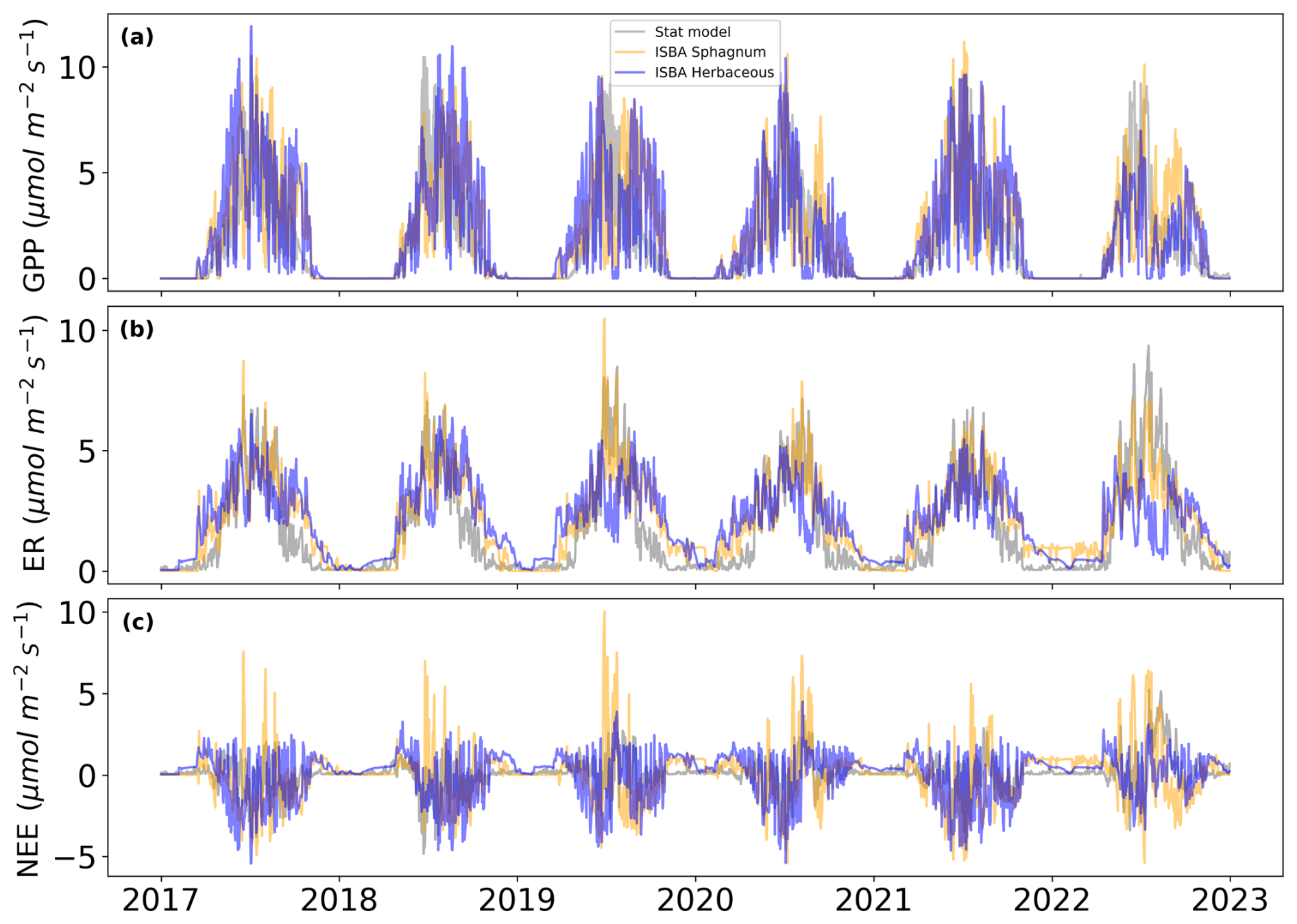
Figure 1 Daily (a) gross primary productivity and (b) ecosystem respiration fluxes compared between statistical models (grey) (Garisoain et al., 2024) and ISBA over the 2017–2022 period for herbaceous (blue) and Sphagnum mosses (orange).

3 Model validation over the 2017–2023 period

Carbon fluxes

Figure 1 compares three time series from 2017 to 2023, illustrating Gross Primary Productivity (GPP), Ecosystem Respiration (ER) and Net Ecosystem Exchange (NEE) modeled by a statistical model (grey) and the ISBA model for Sphagnum (orange) and Herbaceous (blue). The top plot (a) shows GPP with r² values of 0.6 and 0.62 (RMSE of 1.9 and 1.6 $\mathrm{\mu }{\mathrm{mol}}^{-\mathrm{2}}{\mathrm{s}}^{-\mathrm{1}}$, see Fig. A4a, b), indicating moderate agreement between the models. The middle plot (b) shows ER with r² values of 0.82 and 0.44 (RMSE of 0.9 and 1.6 $\mathrm{\mu }{\mathrm{mol}}^{-\mathrm{2}}{\mathrm{s}}^{-\mathrm{1}}$, Fig. A4d, e), revealing stronger agreement for ER, particularly for Sphagnum respiration. The bottom plot, Fig. A4c, f, shows NEE with r² values of 0.1 and 0.2 (RMSE of 1.6 and 1.3 $\mathrm{\mu }\mathrm{mol}{.}^{-\mathrm{2}}{\mathrm{s}}^{-\mathrm{1}}$). Additional scatter plots for the mixed vegetation configuration (Fig. A4g–i) highlight contrasted performances across fluxes. For GPP, the mixed simulation shows a level of agreement comparable to that of herbaceous vegetation alone (r²=0.62, RMSE = 1.58 $\mathrm{\mu }{\mathrm{mol}}^{-\mathrm{2}}{\mathrm{s}}^{-\mathrm{1}}$). For ER, the mixed configuration exhibits an intermediate performance, but with a substantial improvement compared to herbaceous vegetation alone (r²=0.60, RMSE = 1.32 $\mathrm{\mu }{\mathrm{mol}}^{-\mathrm{2}}{\mathrm{s}}^{-\mathrm{1}}$). For NEE, the mixed simulation yields higher skill scores (r²=0.24, RMSE = 1.17 $\mathrm{\mu }{\mathrm{mol}}^{-\mathrm{2}}{\mathrm{s}}^{-\mathrm{1}}$) than either vegetation type considered separately, although overall correlations remain low.

The ISBA model captures the interannual variability of GPP, ER and NEE effectively (Fig. A5), Consistently showing slightly higher values at the beginning of the growing season, much higher values at the end of the growing season, and stronger winter ecosystem respiration (ER) compared to the statistical model. Herbaceous vegetation is more sensitive to summer droughts than Sphagnum, leading to reduced GPP and ER in summer, especially during the 2022 drought, which caused a sharp decline in herbaceous GPP and ER.

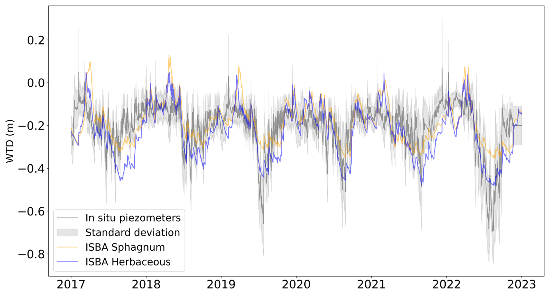
Figure 2 Hourly in situ mean water table depth is shown in grey, with its standard deviation in shaded areas, compared to the hourly diagnosed water table depth of ISBA over the 2017–2022 period for two different types of vegetation herbaceous (blue) and Sphagnum mosses (orange).

3.0.1 Water table depth

Figure 2 compares the mean water table depth (WTD) from in situ measurements (grey with shaded standard deviation) to the ISBA diagnosted WTD (orange for Sphagnum mosses and blue for herbaceous) over the period 2017–2022. The ISBA model generally follows the observed data, capturing the overall trends and seasonal variations (Fig. A5) in WTD although there are occasional deviations, particularly at the end of the growing season and during drought events where the observed data shows higher variability. Overall, the ISBA model demonstrates rather satisfactory performance in simulating WTD (r²=0.47, RMSE=0.09 m for herbaceous, r²=0.33, RMSE=0.1 m for Sphagnum and r²=0.45, RMSE=0.09 m for the mixed vegetation, Fig. A6). The simulated WTD with herbaceous plants is consistently lower than with Sphagnum mosses.

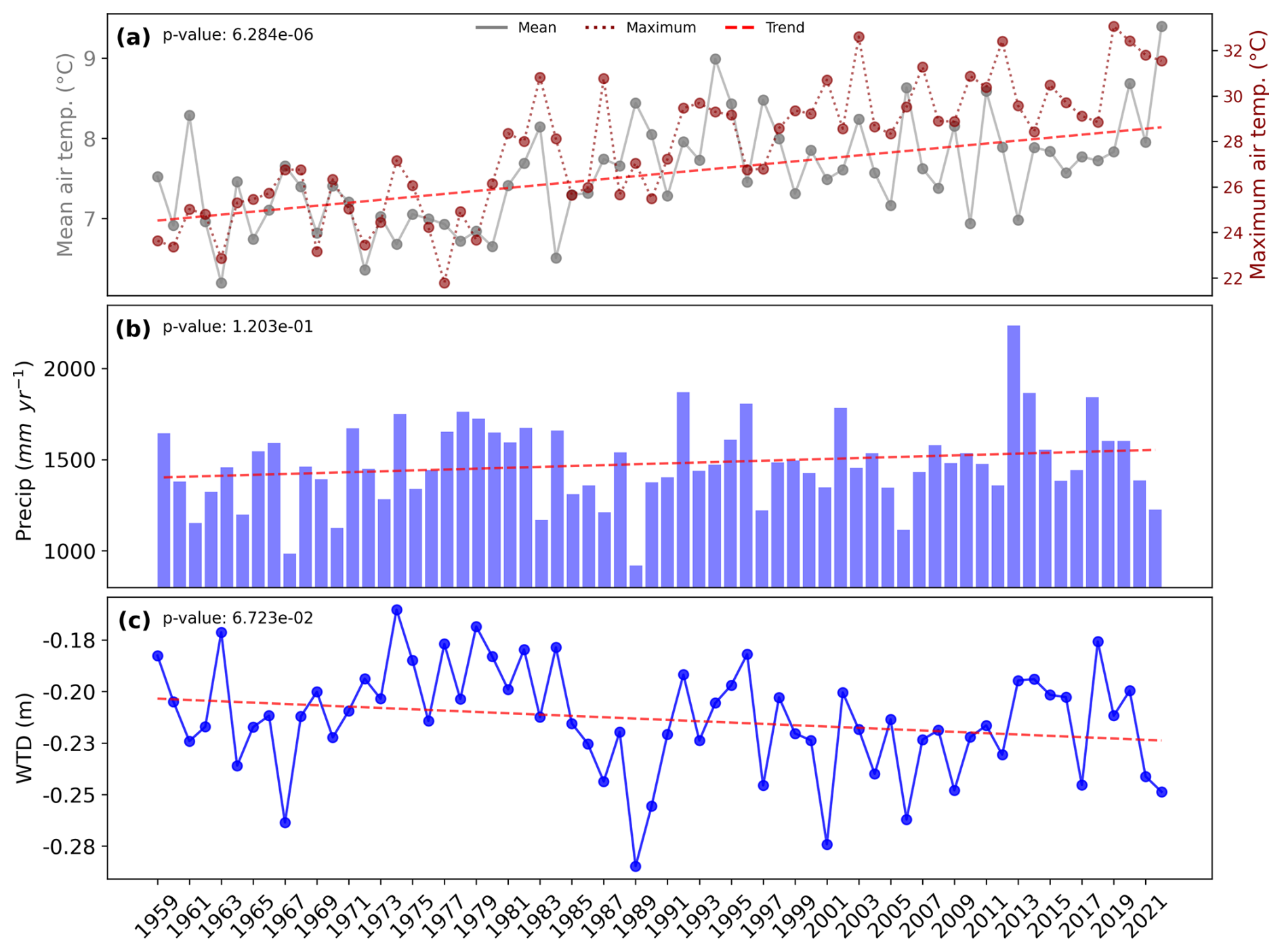
Figure 3 (a) Mean and maximum annual air temperature (°C) and (b) annual cumulate precipitation mm yr⁻¹ both from the S2M reanalysis and (c) mean water table depth (m) diagnosed from ISBA outputs, along with their trends as red dashed lines and corresponding p values.

4 Results: Water and carbon balance of the peatland over the last 60 years

4.1 Environmental variables

Figure 3 consists of three panels, labeled (a), (b), and (c), illustrating the evolution of mean and maximum annual temperature, annual cumulative precipitation, and annual mean water table depth (diagnosed from ISBA) from 1959 to 2022, along with their respective trends and p values. Annual mean temperature (a) shows a significant (p value <0.05) increasing trend over the years. The annual mean temperature increases from approximately 7 °C in the early years to about 9 °C by 2022. Annual maximum temperature shows a similar evolution with an increase up to 8 °C from 1959 to 2022.

Annual cumulative precipitation (b) ranges from approximately 1000 to 2250 mm, while the Water Table Depth (WTD) (c) varies between −0.16 and −0.29 m over the whole period. A steady increase in the level of the water table is observed from 1967 to 1983, followed by a sharp decline, reaching its minimum in 1989. After this, the WTD rises again and stabilizes, although notable interannual fluctuations persist until the end of the period. Interestingly, the fluctuations in annual precipitation closely mirror those of the mean annual WTD, suggesting a strong correlation between these two variables. The trends of annual cumulative precipitation and annual mean WTD move in opposite directions, with precipitation increasing and the level of the water table decreasing. However, both trends are not significant (p values >0.05).

4.2 Net ecosystem exchanges

This section analyzes long term NEE dynamics and their drivers using ISBA simulations forced by the S2M reanalysis. Unless stated otherwise, all simulations and analyses presented in this section use the site vegetation distribution derived from Henry et al. (2014), i.e., 70 % herbaceous plants and 30 % Sphagnum mosses.

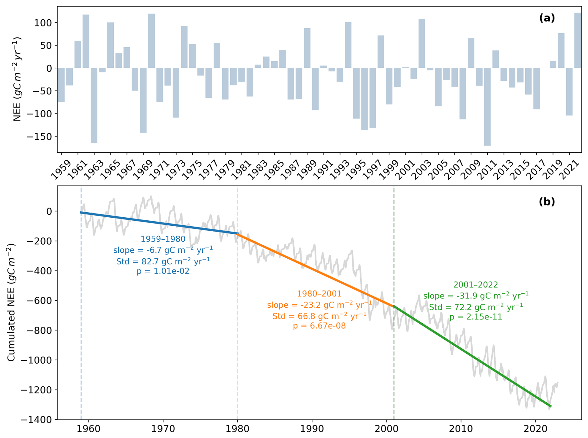
Figure 4 (a) Annual net ecosystem exchange ($\mathrm{g}\mathrm{C}{\mathrm{m}}^{-\mathrm{2}}\mathrm{yr}-\mathrm{1}$) from 1959 to 2022, as simulated by ISBA. (b) Hourly cumulated net ecosystem exchange (g C m⁻²) from 1959 to 2022, also from ISBA. The pannel additionally reports the linear trend (slope), its p value, and the standard deviation of annual NEE for three distinct periods: 1959–1980, 1980–2001, and 2001–2022.

4.2.1 An overall carbon sink despite strong inter-annual variability

Figure 4 illustrates (a) the annual Net Ecosystem Exchange (NEE) and (b) the cumulative NEE from 1959 to 2022. The lowest annual NEE is modelled in 2011 (−171 $\mathrm{g}\mathrm{C}{\mathrm{m}}^{-\mathrm{2}}{\mathrm{yr}}^{-\mathrm{1}}$), while the highest value occurs in 2022 (122 $\mathrm{g}\mathrm{C}{\mathrm{m}}^{-\mathrm{2}}{\mathrm{yr}}^{-\mathrm{1}}$). Panel (b) shows a long-term decrease in cumulative NEE, indicating that the ecosystem acts as a net carbon sink over the entire study period. Piecewise linear trends computed for three successive 22 year periods (1959–1980, 1980–2001, and 2001–2022) reveal a progressive intensification of carbon uptake, as evidenced by increasingly negative slopes of cumulative NEE. The comparison of slopes between periods indicates that this intensification is not linear through time. The strongest increase in carbon sequestration occurs between the first and second periods, while the rate of intensification decreases after the early 2000s, suggesting a slowdown in the acceleration of the carbon sink despite continued strengthening.

Interannual variability, quantified by the standard deviation of annual NEE and reported as text annotations for each period, shows a marked temporal evolution. Variability is highest during the early period (1959–1980), decreases substantially during the phase of strongest sink intensification (1980–2001), and slightly increases again during the most recent period (2001–2022). This pattern suggests that the period of rapid carbon sink strengthening coincides with a more stable interannual behaviour, whereas recent decades combine sustained carbon uptake with a renewed increase in year-to-year variability.

Overall, despite substantial annual fluctuations, the long term signal remains robust and highlights a persistent accumulation of carbon by vegetation over the past six decades.

4.2.2 Seasonality of GPP, ER and NEE over the 1959–2022 period

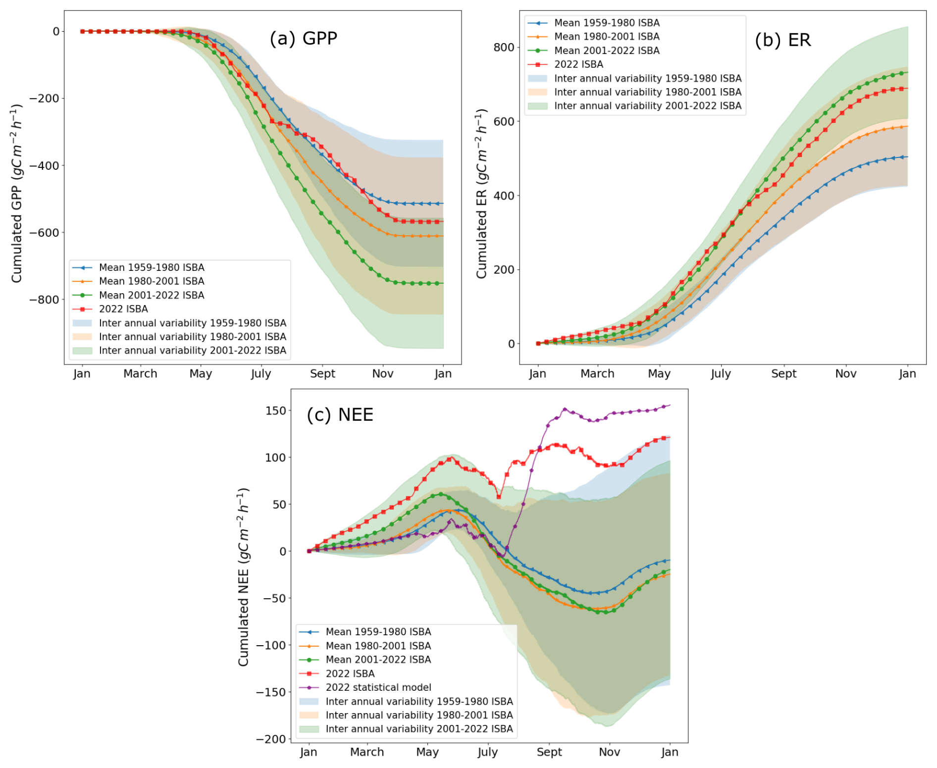
Figure 5 Seasonal evolution of cumulated (a) gross primary productivity (shown with negative sign by convention), (b) ecosystem respiration, (c) net ecosystem exchanges from ISBA over several time periods: 1959–1980 in blue, 1980–2001 in orange, 2001–2022 in green with interannual variability represented as a 90 % confidence interval. Superimposed, the 2022 NEE seasonality simulated by ISBA (red curve) and the statistical model (purple curve).

Figure 5 depicts the seasonal mean and interannual variability in gross primary production (a), ecosystem respiration (b), and net ecosystem exchange (c) over several time periods, specifically 1959–1980 (blue), 1980–2001 (orange), and 2001–2022 (green), with a focus on the year 2022 both from ISBA (red line) and the statistical model (purple line). Periods of approximately 22 years were chosen to ensure statistically robust trend estimates, following common climatological practice for analysing multi-decadal variability. Given the 64 year length of the record, three successive periods were defined with a slight overlap, allowing each period to be long enough for robust linear trends while maintaining three comparable intervals (World Meteorological Organization, 2017). Each subplot shows cumulative values with their respective mean and interannual variability at 90 % confidence interval. In panel (a), GPP values are negative, indicating carbon uptake by vegetation, with more pronounced uptake during the growing season (April to September). Panel (b) shows ER values, which are positive, representing carbon release. Respiration increases during warmer months, with higher rates, suggesting intensified ecosystem respiration. Panel (c) combines GPP and ER to show NEE. The GPP intensifies over time and becomes increasingly pronounced across the three periods. The same trend is observed for respiration. As a combination of these two variables, NEE exhibits greater seasonal variability, which is not necessarily easy to grasp from this graph but is more apparent in Fig. 6. The mean NEE values for the periods 1980–2001 and 2001–2022 show a similar trend, except during winter, when the NEE of the 2001–2022 period shifts towards positive values. Nonetheless, over the annual cycle, both of these periods display more negative NEE values compared to the 1959–1980 period.

The seasonality of GPP (a) and ER (b) has gradually intensified over time, as observed in the three periods. For NEE (c), the trend is less straightforward, but its seasonality has become increasingly pronounced. Additionally, the duration of the growing season has extended, as reflected by the earlier spring and later summer inflection points of cumulative NEE (solid blue, orange and green curves (panel c)).

Focusing on 2022, the NEE curve (red) deviates entirely from the interannual variability of the three periods combined, starting in July and continuing through November. Comparing this with the statistical model for 2022 (purple curve), we observe that despite differences in seasonality between ISBA and the statistical model, both agree in highlighting 2022 as a year significantly outside the confidence intervals. While GPP and ER for 2022 remain within the 2001–2022 interannual variability, the GPP is notably close to the lower limit (− GPP to the upper limit), underscoring the exceptional nature of this year in terms of carbon flux dynamics.

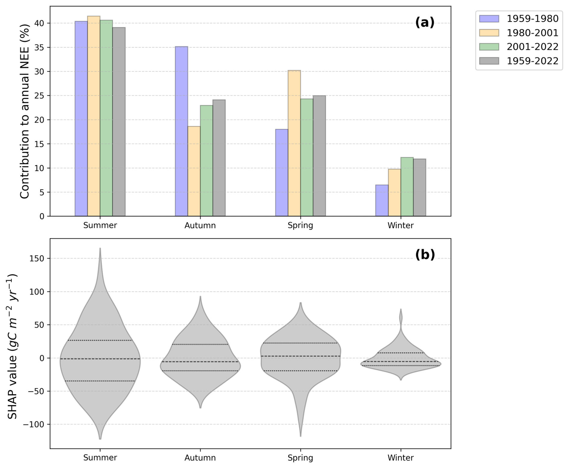
Figure 6 (a) Seasonal contributions to annual NEE across four time periods: 1959–1980 in blue, 1980–2001 in orange, 2001–2022 in green, 1959–2022 in grey. Each bar represents the relative importance of a season in explaining the total NEE, as determined by Shapley regression coefficients. Seasons are defined as winter (December–February), spring (March–June), summer (July–August), and autumn (September–November). (b) Distribution of SHAP values by season for 1959–2022. Positive or negative SHAP values indicate the direction of each season's contribution to annual NEE, showing whether a season increases or decreases the yearly flux.

Figure 6a shows that across all time periods, summer is the season contributing the most to annual NEE variability, accounting for approximately 39 % of the total contribution over the 1959–2022 period. Autumn and spring follow, alternating in second place depending on the period, with comparable contributions of around 23 %–25 %. Winter consistently exhibits the lowest contribution, around 11 % of the annual NEE variability. The distribution of signed SHAP values for the full period (Fig. 6b) further highlights the seasonal dynamics. Summer displays a wide variability, with the median and central 50 % of values slightly below zero, but with long positive tails reflecting years with strong CO₂ release to the atmosphere. Autumn is generally shifted toward positive values, with extreme positive contributions in some years. Spring is centered slightly below zero, with extremes toward negative values. Winter shows relatively low variability, with a skewed distribution including many negative contributions but a long positive tail, indicating occasional meaningful contributions despite its overall smaller role. Overall, these results confirm that summer dominates the interannual variability of annual NEE, but also reveal that other seasons particularly autumn and spring can contribute substantially in certain years. This supports the focus on summer NEE drivers while recognizing the importance of seasonal context.

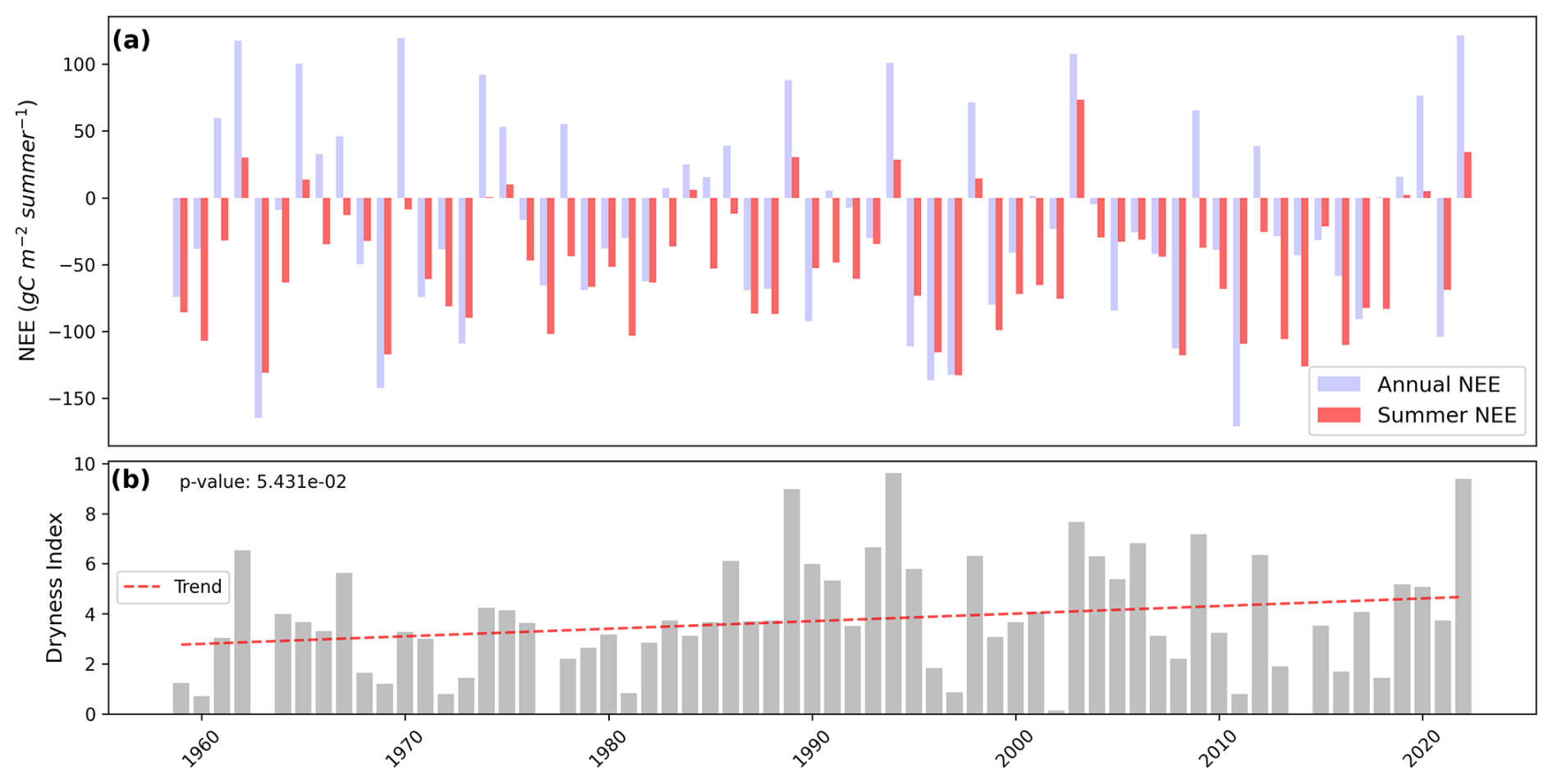
Figure 7 (a) Summer net ecosystem exchanges (in red) compared to annual (in blue) from 1959 to 2022, as simulated by ISBA. (b) Dryness index, derived from water table depth combining ISBA outputs and S2M reanalysis data, from 1959 to 2022 with its trend as red dashed line and associated p value.

4.3 Joint Influence of Air Temperature and Water Table Depth on Summer NEE Variability

Panel (a) of Fig. 7 shows the evolution of cumulative summer NEE (red) compared to cumulative annual NEE (blue) from 1959 to 2022. The cumulative summer NEE tends to “drive” the cumulative annual NEE almost always sharing the same sign, except in years near equilibrium (cumulative annual NEE = 0). This relationship is supported by a strong correlation between summer and annual cumulative NEE (r²=0.71, Fig. A7) and by the fact that summer NEE contributes approximately 40 % of the interannual variability of cumulative NEE (Fig. 6).

Panel (b) illustrates the evolution of the dryness index from 1959 to 2022. The trend shows an increasing pattern, with p=0.054, which is slightly above the conventional significance threshold of 0.05. As the dryness index increases, the cumulative summer NEE also increases, showing a good correlation (r²=0.6, Fig. A8). The dryness index exceeded 6 in only one year from 1959 to 1980, in five years from 1980 to 2001, and in six years from 2001 to 2022. This suggests an increase in the frequency of high dryness index episodes, indicating a rising frequency of summer droughts. Four years also stand out with particularly high dryness index values: 1989, 1994, 2003, and 2022, all of which occurred after the 1980s.

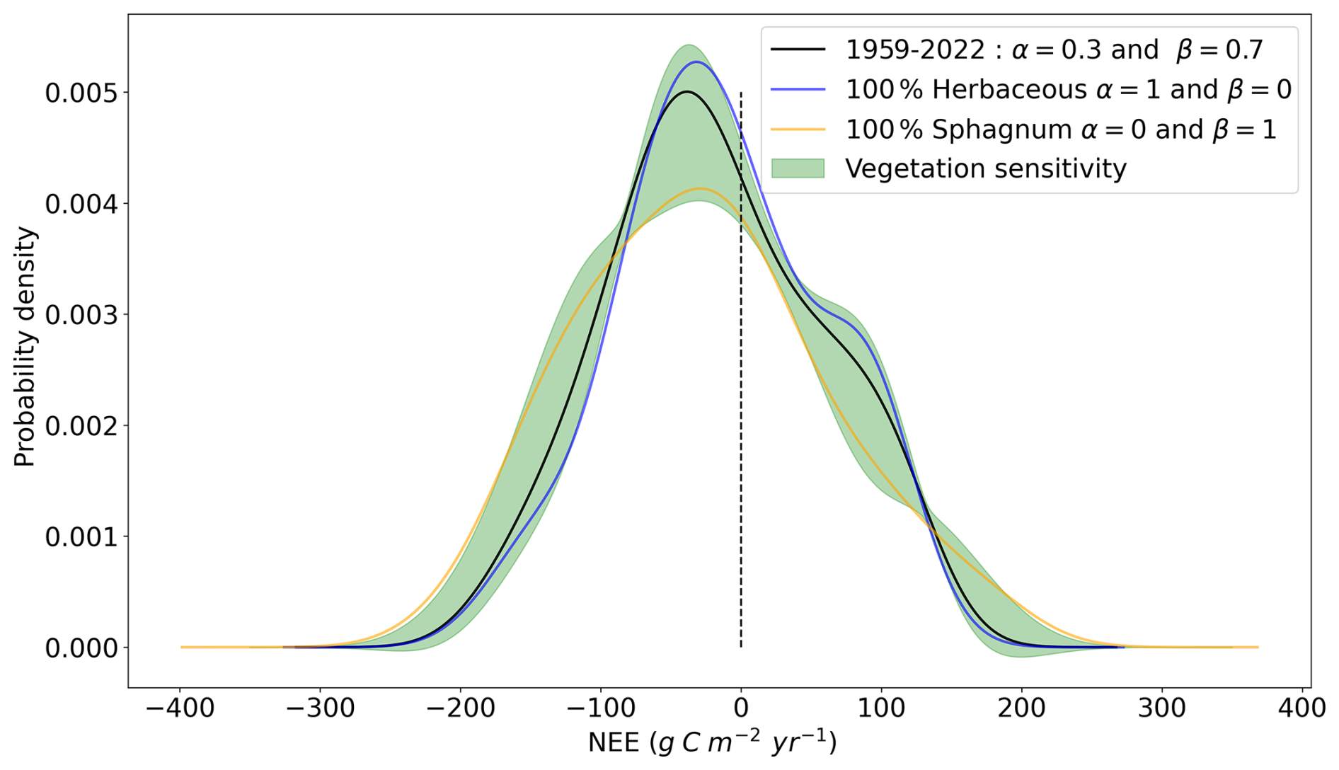
Figure 8 Probability density function of annual cumulated net ecosystem exchange over 1959–2022. In black, the vegetation mix corresponds to 70 % herbaceous and 30 % Sphagnum. In orange a 100 % Sphagnum mix and in blue a 100 % herbaceous mix. In shaded areas, the 95 % confidence intervals corresponding to the variation of the vegetation mix in the form $\mathit{\alpha }\times {\text{NEE}}_{\mathrm{Sphagnum}}+\mathit{\beta }\times {\text{NEE}}_{\mathrm{herbaceous}}$ with $\mathit{\beta }=\mathrm{1}-\mathit{\alpha }$ and α varying from 0 to 1 in steps of 0.01.

4.4 Vegetation sensitivity

Figure 8 highlights the changes in the distribution of the annual cumulated Net Ecosystem Exchange (NEE) over 1959–2022. The black curve represents the probability density of NEE for a vegetation mix of 70 % herbaceous and 30 % Sphagnum, with shaded regions representing the 95 % confidence intervals accounting for variations in vegetation composition.

We observe that while the overall shape of the annual cumulative NEE probability density remains largely unchanged, significant differences arise depending on the vegetation type, particularly around the peak of the distributions. Sphagnum mosses amplify NEE extremes, either enhancing CO₂ absorption by vegetation or increasing CO₂ release to the atmosphere, resulting in a flatter distribution compared to herbaceous vegetation. In contrast, herbaceous plants have a buffering effect, with a distribution more concentrated around the main peak and a secondary, smaller peak slightly below +100 $\mathrm{g}\mathrm{C}{\mathrm{m}}^{-\mathrm{2}}{\mathrm{yr}}^{-\mathrm{1}}$, resulting in a bimodal pattern. These findings highlight the importance of considering different vegetation types, as they respond differently to changing environmental conditions. For completeness, the corresponding figures for GPP and ER are provided in the Appendix (Fig. A10).

5 Discussions

5.1 Model validation and vegetation sensitivity

The primary objective of this study was to evaluate the newly implemented Sphagnum PFT in the ISBA land surface model. Sphagnum photosynthetic activity is linked to water content in the top 10 cm of soil. While the model reproduces site scale carbon fluxes reasonably well given observational constraints, a more detailed validation of the water cycle would require eddy covariance data and multi site evaluations to assess parameter transferability. The aim was not to optimize parameters, but to test whether realistic behavior could be reproduced at a well instrumented site using literature derived values.

The mixed representation, combining Sphagnum and herbaceous PFTs, accounts for contrasting responses to soil moisture. We removed the influence of soil moisture on respiration (θ(z)) for Sphagnum, allowing the moss layer to maintain microbial activity under dry conditions, while it was retained for herbaceous layers to preserve the soil moisture sensitivity of heterotrophic respiration. Although respiration from the herbaceous component alone is not improved, retaining θ(z) is consistent with previous validations of the ISBA model for herbaceous vegetation, ensuring the parameterization remains grounded in established formulations (Gibelin et al., 2008). Importantly, the combination of PFTs captures contrasting responses to soil moisture, introducing functional diversity that likely increases the robustness of ecosystem carbon fluxes. This mechanism is reflected in the observed modest improvement of NEE on the mixed vegetation dataset, even if GPP and respiration alone do not always show large gains. These results also highlight the broader uncertainty in representing heterotrophic respiration as a function of soil moisture: classical formulations derived from mineral soils may not adequately capture responses in organic soils, as noted in other peatland modeling studies (Qiu et al., 2019; Guenet et al., 2024), emphasizing the need for further research on moisture/respiration parameterizations.

By combining PFTs with contrasting functional responses, the model captures compensatory dynamics across vegetation types: herbaceous layers respond strongly to moisture deficits, while Sphagnum maintains near surface moisture and microbial activity. This functional diversity improves site scale carbon flux estimates and suggests increased model robustness under variable hydrological conditions, which could be further enhanced by including interactive dynamics between Sphagnum mosses and herbaceous following the work of Kim and Verma (1996) but also competition and coupled carbon/water processes (Lippmann et al., 2023; Heijmans et al., 2008; Wu and Blodau, 2013a; Gong et al., 2020).

5.2 The key predictors of annual net ecosystem exchange (NEE)

The methodology developed in this study aimed to investigate the variability and evolution of carbon fluxes in the Bernadouze peatland from 1959 to 2022 using a CSM validated for the present period (2017–2022). This approach provides insight into the long-term functioning of the peatland on a century-scale timescale, which has been scarcely explored in the literature due to the lack of suitable tools. This novel methodology provides access to an unprecedented temporal scale, enabling current observations to be interpreted within a broader historical perspective.

Over the past 64 years, the Bernadouze peatland has shown marked variability in net ecosystem exchange (NEE), while overall maintaining its role as a carbon sink. This variability is strongly influenced by climatic and hydrological conditions, particularly precipitation, water table dynamics, and air temperature, as highlighted in previous research (Yurova et al., 2007; Laine et al., 2019). The reconstruction of water table height, together with the development of a dryness index that integrates both air temperature and water table depth, offers a robust explanation for the observed fluctuations in carbon fluxes, as also supported by other studies (Helbig et al., 2022). Vapor Pressure Deficit (VPD) is generally an important factor to consider, particularly for vegetation development, as it influences both GPP and plant transpiration (Fu et al., 2022). However, at the Bernadouze site, VPD is low and exhibits little variation (Figure A9 (a)), suggesting it has a limited effect on NEE. Furthermore, VPD is strongly correlated with temperature, which captures much of its potential influence. A recent study in Northern Hemisphere peatlands (Chen et al., 2023) also indicates that VPD has a neutral effect on vegetation and does not necessarily induce stomatal closure in vascular plants. The humid conditions at the site, along with the presence of bryophytes, help satisfy atmospheric water demand. Overall, air temperature and water table depth remain the primary drivers explaining NEE variability.

It is also observed that, in Bernadouze, summer NEE is the dominant contributor to the annual carbon balance, though the relative influence of other seasons varies across time periods. In recent decades, transitional seasons such as spring and autumn have become increasingly significant compared to earlier years. Understanding how climate change influences NEE seasonality offers key insight into the complex dynamics of carbon fluxes and the shifting balance between source and sink processes throughout the year, as also emphasized by Helbig et al. (2022). The dryness index developed in this study also appears to be a good proxy for summer NEE and, consequently, for annual NEE (Figs. A8 and A7). On other peatland sites where carbon flux measurements are not available, this index could potentially serve as a preliminary source of information to estimate the carbon balance of peatlands.

5.3 Climate change and droughts episode

Over the past 64 years, the Bernadouze peatland has experienced an increasing frequency of severe droughts, as indicated by the calculated dryness index (Figs. 7b and A3b). These events have contributed to the destabilization of the NEE balance, particularly in 2022. Despite some differences in seasonal representation, both ISBA and the statistical model by Garisoain et al. (2024) agree that from July to November 2022, conditions fell completely outside the range of interannual variability. Similar dry summers have occurred in the past, notably in 1989, 1994, and 2003, and have consistently led to significant CO₂ emissions into the atmosphere. The years 1989 and 2003 are recognized as having experienced different types of drought conditions in France, ranging from multi-year precipitation deficits (1989–1990) to short, hot, and dry periods (2003) (Vidal et al., 2010). Similarly, 1994 is also identified as a year with a hot summer, preceded by a winter precipitation deficit in Southern Europe (Vautard et al., 2007). The dryness index effectively captures these hot and dry summers, which impact vegetation, its development, and consequently, the NEE flux.

As the growing season lengthens and GPP increases due to rising air temperatures, a compensatory effect appears to be at play. The peatland's greening and higher summer GPP fluxes currently help mitigate the impact of droughts, allowing it to remain a carbon sink. Over the 2001–2022 period, spring and autumn have played a growing role in shaping annual NEE, suggesting that these transitional seasons, along with winter, may become increasingly influential in the future, potentially counterbalancing summer carbon losses. However, the longevity of this balance remains uncertain. Some years, in our data, show a partial imbalance, indicating that the compensatory effect may not always fully buffer extreme conditions. Similar patterns have been observed in European forest ecosystems (van der Woude et al., 2023), where compensatory mechanisms were insufficient to maintain carbon balance; this provides a useful analogy for interpreting the partial signals we observe in our peatland data. While greening and seasonal compensation currently mitigate summer carbon losses, prolonged or intensified droughts in the future could challenge this balance and affect the peatland’s long term carbon sink function.

The significant increase in annual maximum temperatures about 8 °C over 64 years raises concerns about the vegetation's ability to withstand such extreme warming. Studies on potential shifts in plant composition under climate change could provide valuable insights into the future of these ecosystems (Antala et al., 2022; Dieleman et al., 2015). This further emphasizes the need to integrate a broader range of plant communities and their interactions into land surface models, to more accurately represent ecosystem dynamics and their role in the carbon cycle.

6 Conclusion

This study highlights the importance of accurately representing Sphagnum mosses in land surface models to simulate peatland carbon dynamics under changing climatic conditions. Validation of the new Sphagnum PFT within the ISBA model showed its ability to reproduce observed carbon fluxes with reasonable agreement. Analysis of the Bernadouze peatland over the past 64 years revealed that while it has remained a net carbon sink, increasing drought frequency and severity, particularly exemplified by the 2022 event, are destabilizing its carbon balance. The findings emphasize the critical role of vegetation composition, hydrological conditions, and seasonal climate dynamics in modulating peatland carbon fluxes. They also suggest that although compensatory mechanisms currently maintain peatland sink function, future intensification of droughts driven by climate change could potentially shift these ecosystems from carbon sinks to carbon sources. This underscores the urgent need to integrate interactive vegetation dynamics and drought responses into land surface models to better project peatland contributions to the global carbon cycle under future climate scenarios.

Appendix A: Figures and tables

Figure A1 Normalised total Sphagnum conductance as a function of Sphagnum water content.

Figure A2 Sphagnum canopy water resistance as a function of Sphagnum water content.

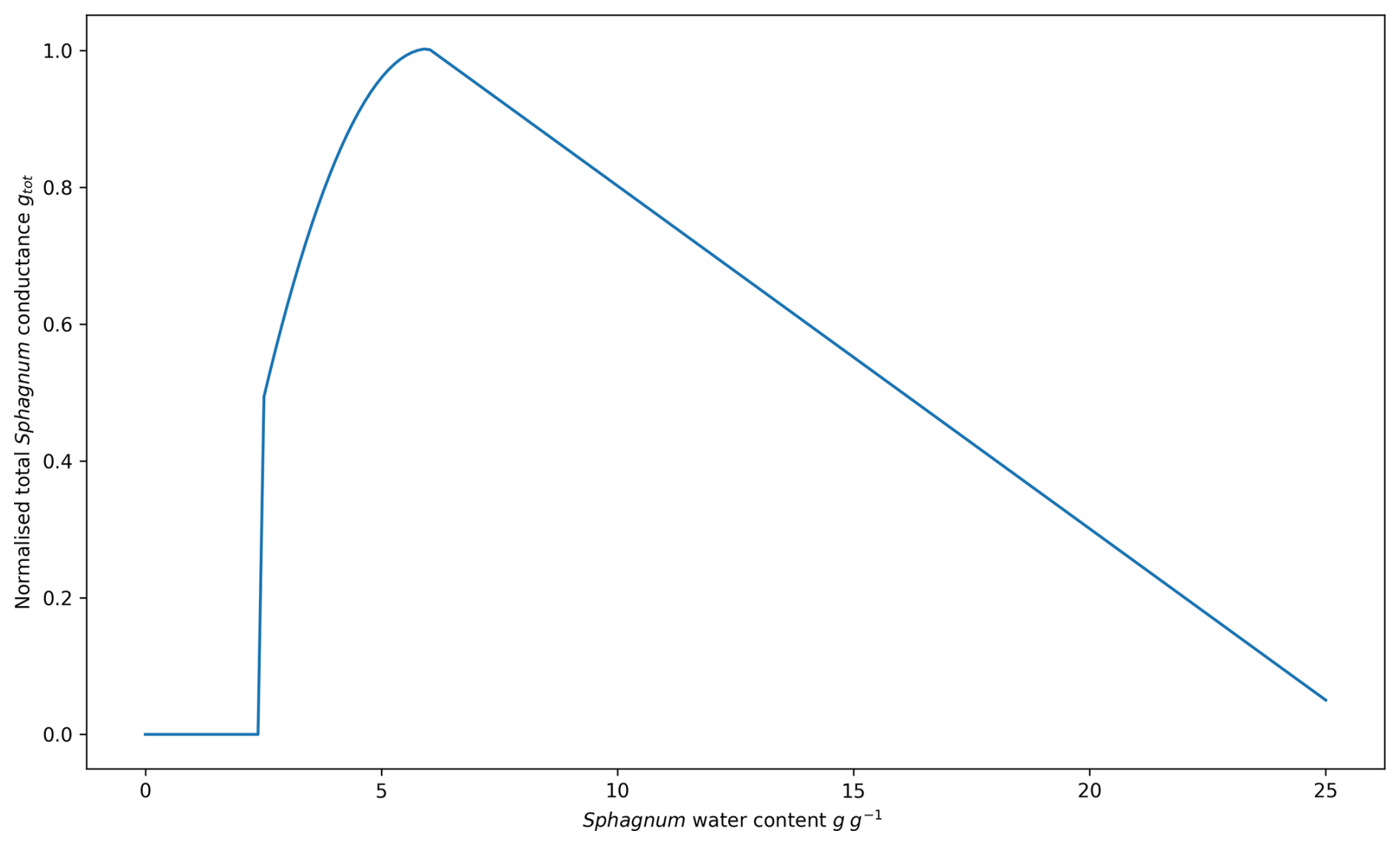
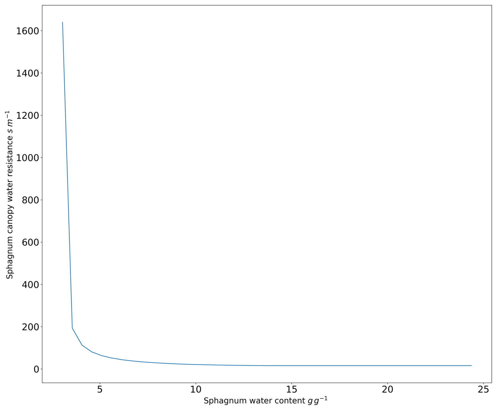
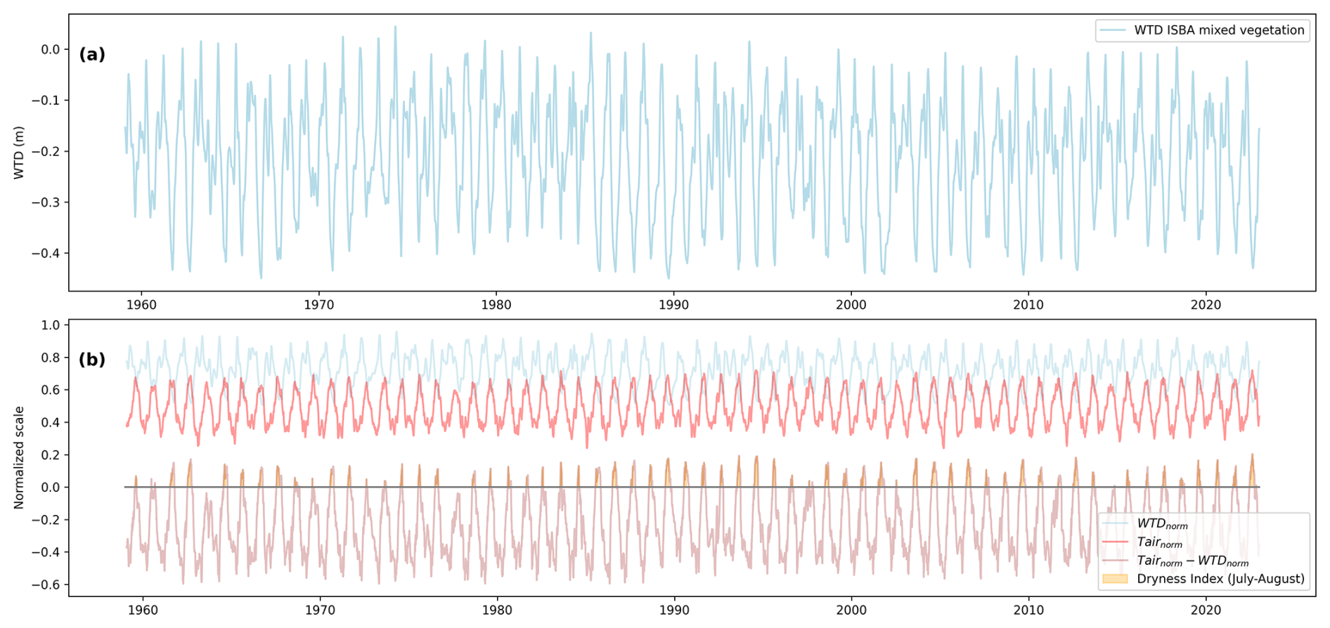
Figure A3 (a) Diagnosed water table depth (WTD) from 1959 to 2022 for the Sphagnum-herbaceous vegetation mix. (b) Light blue: normalized WTD, red: normalized air temperature (Tair), pink: normalized Tair minus normalized WTD, dark blue area under the curve represents the dryness index (DI). Normalization of each variable (X) was done following $X_{\mathrm{normalized}}=\frac{X\mathrm{-}{X}_{\min }}{X_{\max }\mathrm{-}{X}_{\min }}$. WTD_min=1 m is taken from observations and not the diagnosed one from ISBA.

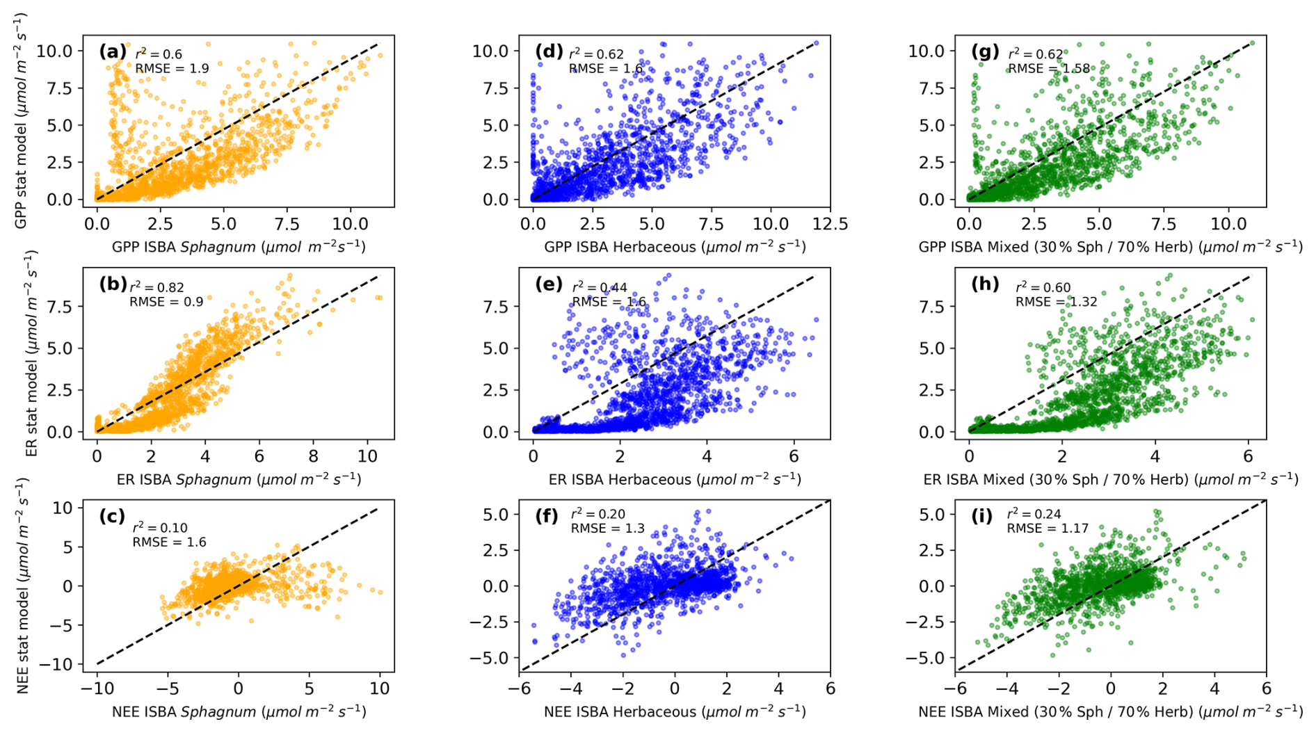
Figure A4 Comparison of daily ecosystem photosynthesis, respiration and net ecosystem exhange from the statistical model with: (a) the new Sphagnum photosynthesis, (b) the new Sphagnum ecosystem respiration, (c) the new Sphagnum net ecosystem exchange, (d) the previous herbaceous photosynthesis, (e) the previous herbaceous ecosystem respiration, (f) the previous herbaceous net ecosystem exchange, (g) the mixed vegetation photosynthesis, (h) the mixed vegetation ecosystem respiration, (i) the mixed vegetation net ecosystem exchange.

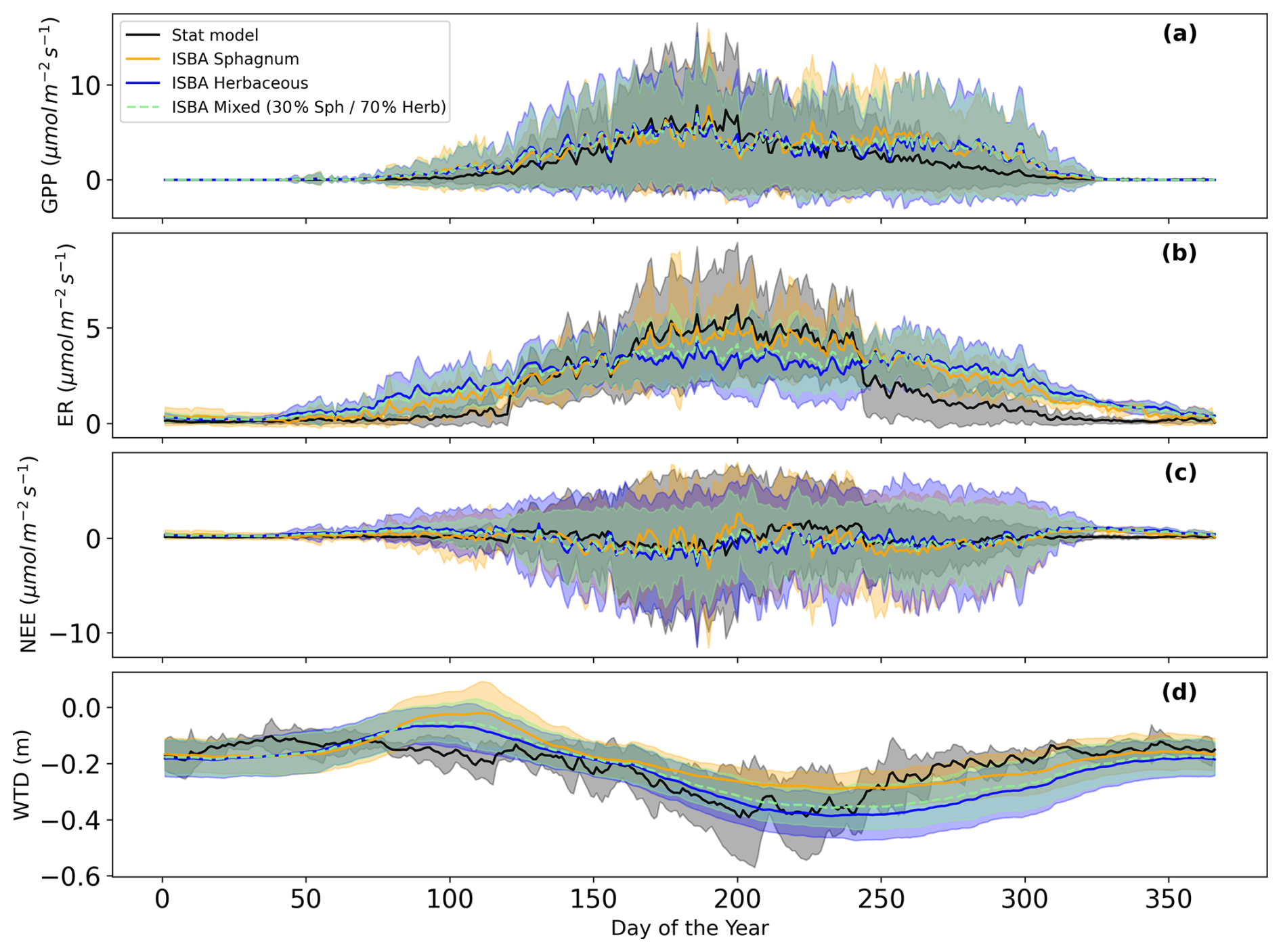
Figure A5 Daily annual cycle (2017–2022) of (a) Gross Primary Productivity, (b) Ecosystem Respiration, (c) Net Ecosystem Exchange, (d) Water Table Depth from the statistical model in black, the ISBA Sphagnum model in orange, the ISBA herbaceous model in blue, and the ISBA mixed vegetation in green.

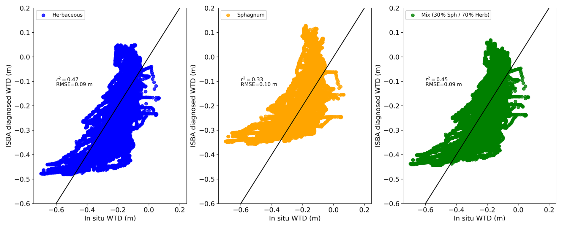
Figure A6 Hourly ISBA-diagnosed water table depth (WTD) with herbaceous vegetation as the dominant cover is compared to hourly in situ WTD in the left panel, while the right panel presents ISBA-diagnosed WTD with Sphagnum as the dominant vegetation versus in situ WTD.

Figure A7 Annual NEE versus Summer NEE for each year from 1959 to 2022.

Figure A8 Summer NEE versus Dryness Index for each year from 1959 to 2022.

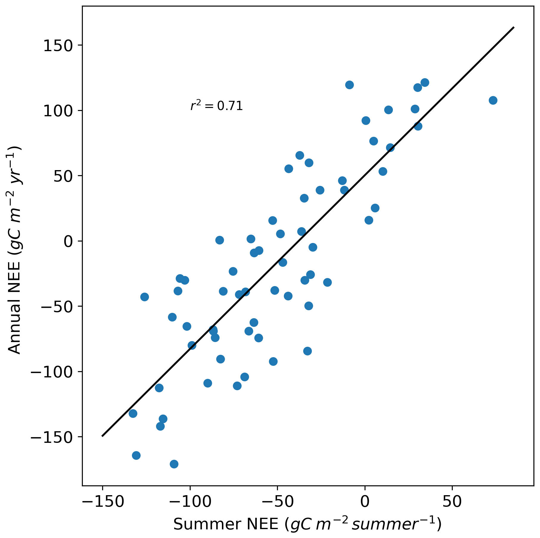
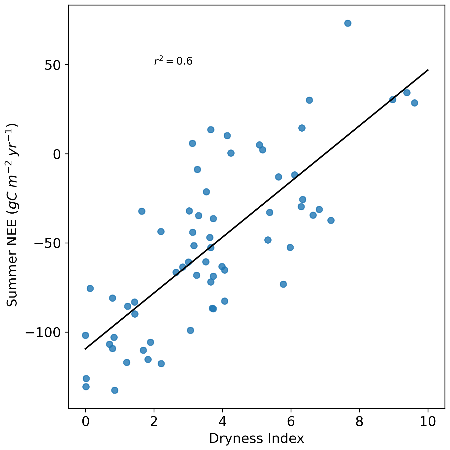
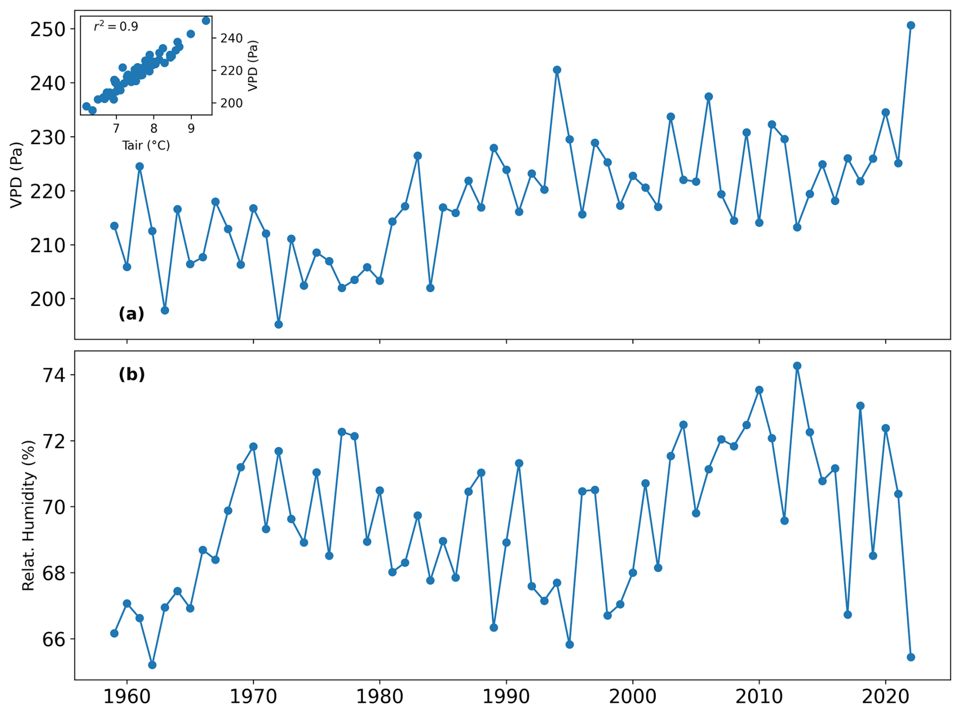
Figure A9 (a) Annual mean of vapor pressure deficit (VPD) (Pa) and scatter plot between VPD and air temperature; (b) Annual mean of relative humidity (%) from 1959 to 2022 derived from the S2M reanalysis.

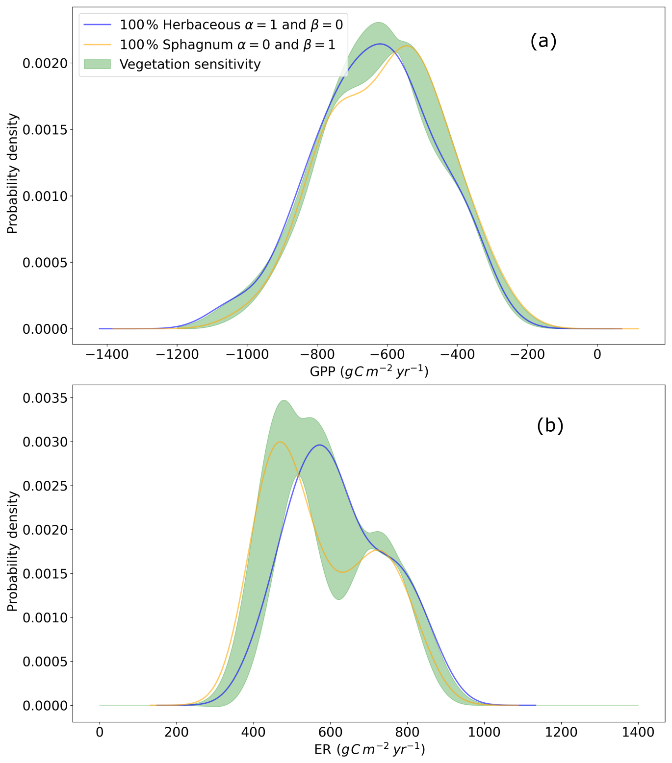
Figure A10 Probability density function of annual cumulated (a) GPP and (b) ER over 1959–2022. In black, the vegetation mix corre- sponds to 70 % herbaceous and 30 % Sphagnum. In orange a 100 % Sphagnum mix and in blue a 100 % herbaceous mix. In shaded areas, the 95 % confidence intervals corresponding to the variation of the vegetation mix in the form $\mathit{\alpha }\times Y_{\mathrm{Sphagnum}}+\mathit{\beta }\times Y_{\mathrm{herbaceous}}$ with β=1−α, α varying from 0 to 1 in steps of 0.01 and Y being GPP or ER.

Table A1 Changes between Sphagnum and C₃ herbaceous plant functional type in ISBA.

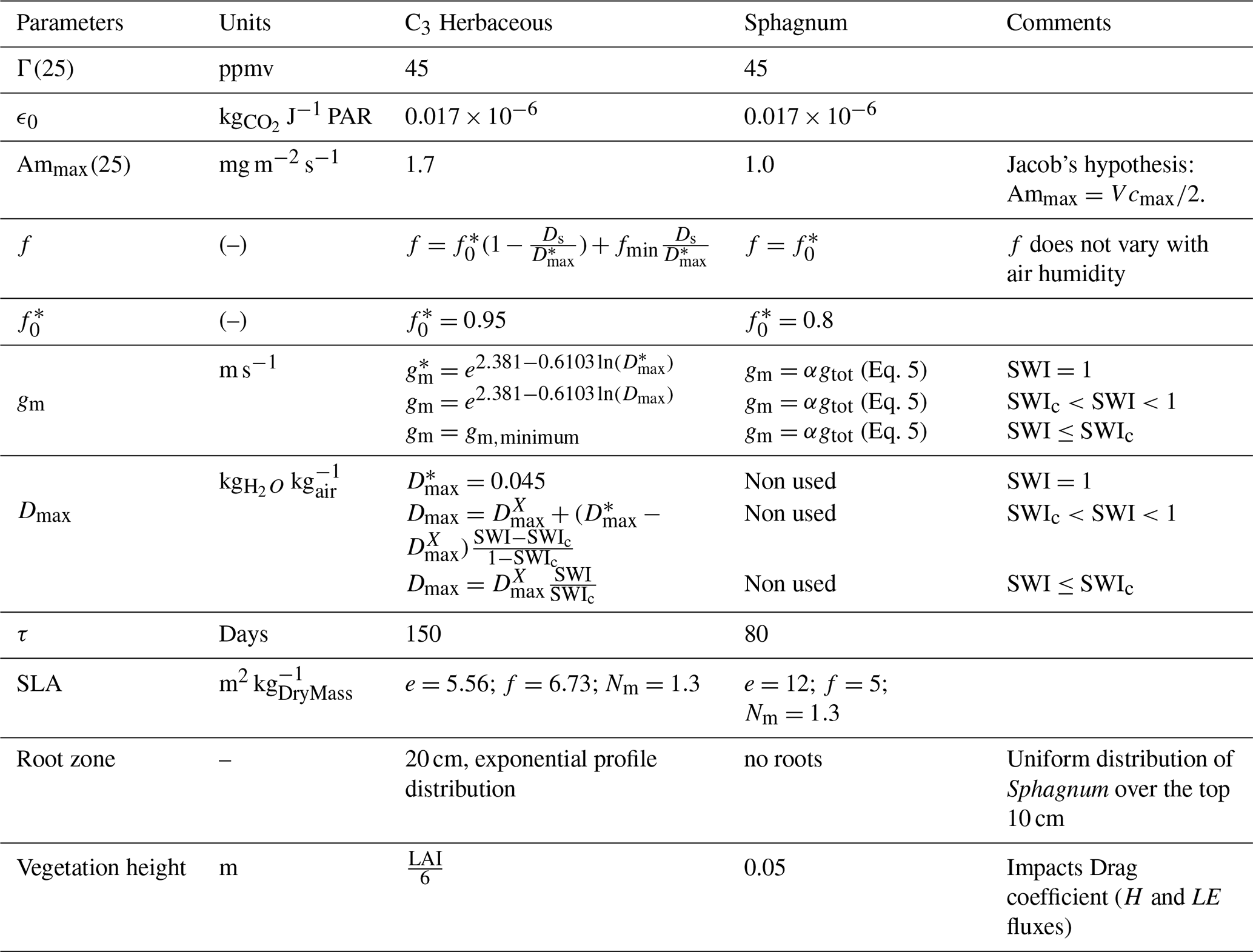
Note 1: $g_{\mathrm{m}}^{*},D_{\max }^{*}$ are the same quantities as g_m,D_max but without hydric stress. Note 2: $D_{\max }^X=\mathrm{0.4}$: this is the maximum value of D_max.

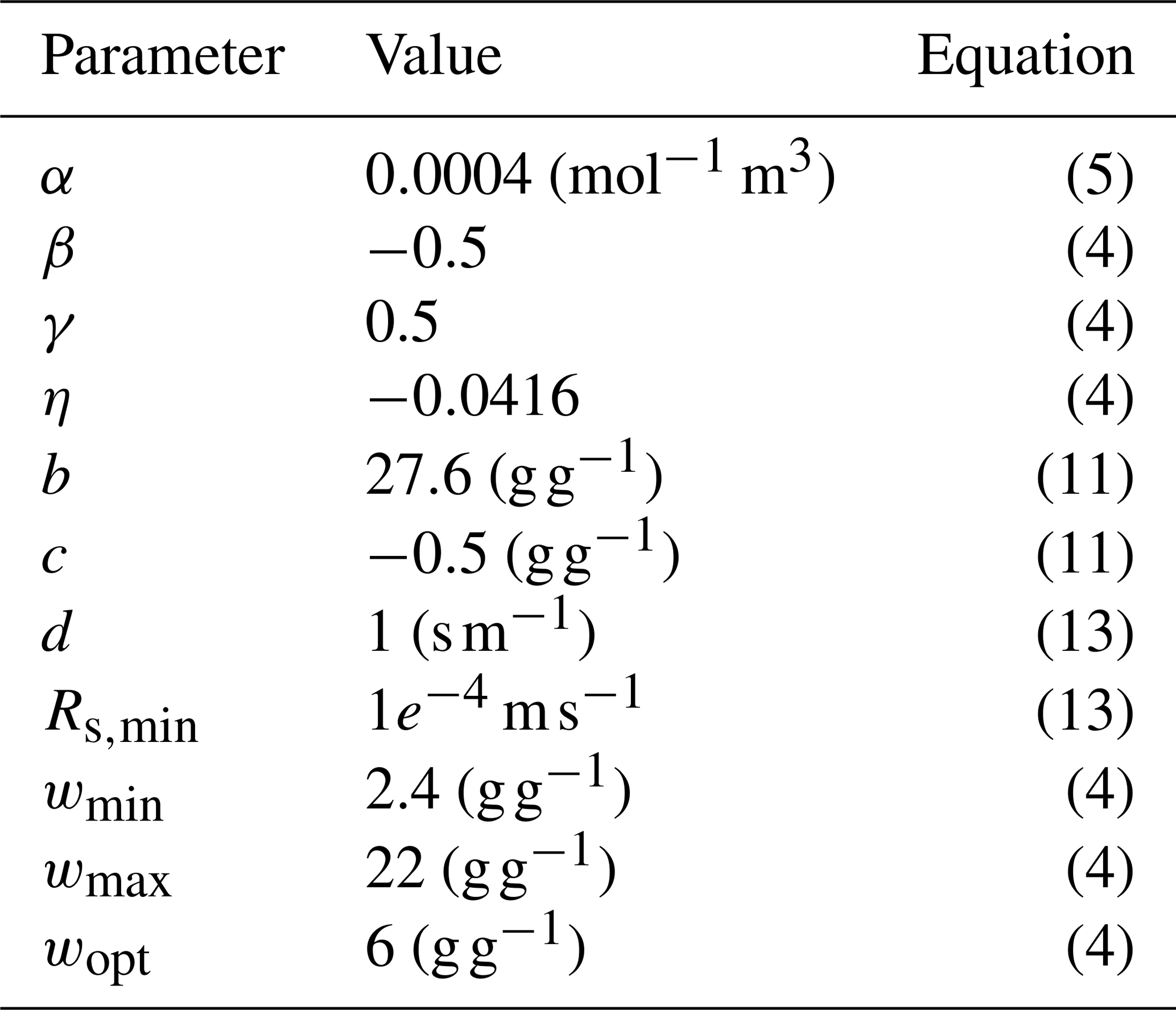
Table A2 Parameters used for the Sphagnum PFT and their associated equations.

Appendix B: ISBA equations

$$\begin{array}{}\text{(B1)}& {\text{Am}}_{\max }\left(T_{\mathrm{s}}\right)={\displaystyle \frac{{\text{Am}}_{\max }\left(\mathrm{25}\right)\times Q_{\mathrm{10}}^{(T_{\mathrm{s}}-\mathrm{25})/\mathrm{10}}}{[\mathrm{1}+\exp [\mathrm{0.3}(T\mathrm{1}-T_{\mathrm{s}})\left]\right[\mathrm{1}+\exp \left[\mathrm{0.3}\right(T_{\mathrm{s}}-T\mathrm{2}\left)\right]}}\end{array}$$

where Am_max(25) is Am_max at 25 °C, Q₁₀ is fixed at 2.0, T_s is the skin temperature in °C and T1 and T2 are reference temperature values. gm in unstressed soil moisture conditions, gm^*, depends on temperature via the same Q₁₀ function as Am_max.

$$\begin{array}{}\text{(B2)}& \mathrm{\Gamma }\left(T_{\mathrm{s}}\right)=\mathrm{\Gamma }\left(\mathrm{25}\right)\times Q_{\mathrm{10}}^{(T_{\mathrm{s}}-\mathrm{25})/\mathrm{10}}\end{array}$$

Γ(25) is Γ at 25 °C. Here Q₁₀ is fixed at 1.5.

$$\begin{array}{}\text{(B3)}& \mathit{ϵ}={\mathit{ϵ}}_{\mathrm{0}}\left({\displaystyle \frac{C_i-\mathrm{\Gamma }}{C_{\mathrm{i}}-\mathrm{2}\mathrm{\Gamma }}}\right)\end{array}$$

ϵ is the initial quantum use efficiency, where ϵ₀ is the maximum quantum use efficiency.

$$\begin{array}{}\text{(B4)}& C_{\mathrm{i}}=f{C}_{\mathrm{a}}+\mathrm{\Gamma }(\mathrm{1}-f)\end{array}$$

The internal CO₂ concentration C_i, is directly derived from the CO₂ concentration in the air C_a and from f which is detailed in Table A1.

$$\begin{array}{}\text{(B5)}& \begin{array}{rl}& E_{\mathrm{g}}=(\mathrm{1}-F_{\mathrm{veg}}){\mathit{\rho }}_{\mathrm{a}}{C}_H{V}_{\mathrm{a}}\left(\mathit{\alpha }{q}_{\mathrm{sat}}\right(T_{\mathrm{s}})-q_{\mathrm{a}})\\ & E_{\mathrm{v}}=F_{\mathrm{veg}}{\mathit{\rho }}_{\mathrm{a}}\left({\displaystyle \frac{\mathit{\delta }}{R_{\mathrm{a}}}}\right)\left(q_{\mathrm{sat}}\right(T_{\mathrm{s}})-q_{\mathrm{a}})\\ & E_{\mathrm{tr}}=F_{\mathrm{veg}}{\mathit{\rho }}_{\mathrm{a}}\left({\displaystyle \frac{\mathrm{1}-\mathit{\delta }}{R_{\mathrm{a}}+R_{\mathrm{s}}}}\right)\left(q_{\mathrm{sat}}\right(T_{\mathrm{s}})-q_{\mathrm{a}})\end{array}\end{array}$$

The evaporation of the vegetated surface is the sum of the evaporation of the soil (E_g) and the evaporation of the vegetation (E_veg): $E=E_{\mathrm{g}}+E_{\mathrm{veg}}$. The evaporation of the vegetation is itself distributed between the direct evaporation (E_v) due to the fraction of folliage covered by water intercepted and the transpiration (E_tr): $E_{\mathrm{veg}}=E_{\mathrm{v}}+E_{\mathrm{tr}}$.

F_veg is the fraction of vegetation, δ the fraction of folliage covered by intercepted water and R_s is the canopy resistance taking into account the upscalling of the cuticular and stomatal resistance.

For the modelling of Sphagnum, δ is set to 0, and R_s is changed in R_sp (in this context, historical transpiration effectively corresponds to the evaporation from Sphagnum).