Glass plate sampling efficiency for trace gases in the sea surface microlayer

Many climate-active trace gases in the atmosphere are closely linked to production and consumption in the ocean, which are, in turn, influenced by the sea surface microlayer (SML). The SML is the upper most layer of the ocean with up to 1 mm thickness, often enriched in organics. Studies of trace gases in the SML aim to identify and quantify potential processes unique to the SML and to understand the SML's influence on the transfer between air and sea. Established sampling techniques of the SML (e.g., glass plate, mesh screen) are associated with high losses for the volatile trace gases. Despite the high losses, in this study we find that meaningful analysis of glass plate samples for the studied trace gases is possible. We experimentally determined the sampling efficiency for the short-lived trace gases dimethyl sulfide (DMS), isoprene, and carbon disulfide (CS₂). Water temperature and trace gas concentration were the main drivers for sampling efficiency variability, while salinity and the number of dips of the glass plate were not significant. The (physicochemical) effect of surface-active substances (surfactants), modelled by the artificial surfactant Triton X-100, could not finally be untangled. Although our results are consistent within our experiments, we do not quantify a sampling efficiency to correct individual measurements, as our experiments did not encompass the full suite of environmental parameters normally encountered in the field, particularly limited to cases of oversaturation. Instead, we discuss using the identified sampling efficiencies of 0.13 ± 0.01 (±standard error) for DMS and isoprene, and 0.12 ± 0.01 for CS₂ as thresholds to identify cases of enrichment in the SML. Future studies should extend to long-lived species (e.g., nitrous oxide, methane), encompass the full range of trace gas saturation, investigate a range of single surfactants as well as mixtures, include the effect of wind, and be repeated for the mesh screen. We hypothesize that a correction of individual measurements requires determining sampling efficiency as a function of environmental parameters, which were limited in the present study.

1 Introduction

Short- and long-lived trace gases impact Earth's climate via processes like hydroxyl radical chemistry, aerosol formation, cloud condensation nuclei formation, or the greenhouse effect. The oceans serve as important sinks and sources for many of these gases. Understanding trace gas cycling in the ocean mixed layer and exchange with the atmosphere across the air-sea interface is, therefore, crucial for climate and air quality predictions. (Liss et al., 2014)

Trace gas data from the upper meter is scarce and the lack of information is even more pronounced for the surface microlayer (SML). The SML is the uppermost layer of the water column with a thickness of less than 1 mm. It often shows organic enrichment, for instance with surface-active substances (surfactants), especially during calm conditions (Wurl et al., 2011). Enrichment is often indicated as enrichment factor (EF), defined as the ratio between the quantity's concentration in the SML and in the underlying water (ULW). Surfactants alter the physicochemical properties of the SML, like reducing the surface tension, and are addressed in most SML studies. When surfactant concentrations are high, so-called slicks form that are often visible as flat surfaces, as they dampen the waves. The SML has been studied for a wide range of physical, chemical and biological parameters, which resulted in the hypothesis of the SML being a biogeochemical reactor (Bibi et al., 2025). However, established sampling techniques are not well suited for volatile gases, causing a severe lack of information on trace gas concentrations directly at the air-sea interface. For ease and convenience, many air-sea gas exchange estimates are thus based on ULW concentrations sampled from the mixed layer (usually around 5 m depth). Studies have shown evidence that this neglect of processes occurring shallower than 5 m and in the SML may be the reason for discrepancies between computed fluxes and predicted or measured fluxes (Booge et al., 2016; Kock et al., 2012; Lennartz et al., 2017; Marandino et al., 2005, 2008). Enrichment of the SML is ubiquitous in the ocean, therefore inaccuracies in air-sea gas exchange estimates may be frequent, leading to subsequent inaccuracies of our understanding of atmospheric chemistry and in climate computations, potentially on a global scale (Sabbaghzadeh et al., 2017; Wurl et al., 2011). To unravel the relevance of the SML on air-sea gas exchange and its potential as a source or sink for trace gases, it is necessary to sample the SML efficiently and accurately.

In order to measure SML concentrations and gradients at sea, samples are often taken by hand with specialized equipment from a small rubber boat, which is less convenient and more difficult than the common underway pumping system or discrete water samples from a CTD rosette used on board during many oceanographic campaigns. A widely used sampling device is the glass plate, which was first described by Harvey and Burzell (1972) for collection of microorganisms and organic content, but other techniques exist as well, such as the mesh screen (Garrett, 1965), rotating drum (Harvey, 1966), membrane sampler (Crow et al., 1975), cryogenic sampler (Turner and Liss, 1985) and more recently a gas-permeable floating tube specially designed for trace gases (Saint-Macary et al., 2023). Several studies discuss the limitations and difficulties to compare results from the different methods for non-volatile compounds (e.g., Cunliffe and Wurl, 2014), while highlighting the need for a new technique to sample volatile compounds, like trace gases (e.g., Engel et al., 2017). There are only a few studies that sampled the SML for trace gases and even fewer that used the glass plate, although it is the most common device used for other parameters measured in the SML. To the best of our knowledge, there are no studies with SML samples for the short-lived trace gas isoprene, and only one on carbon disulfide (CS₂) (Turner and Liss, 1985), but dimethyl sulfide (DMS) measured from SML samples has been used more widely to determine EF (see Saint-Macary et al., 2023; Turner and Liss, 1985; Walker et al., 2016; Yang, 1999; Yang et al., 2001). In those and similar studies, glass plate and mesh screen sampling are usually described as being prone to sampling losses due to volatilization, but to the best of our knowledge the magnitude of the losses has not been tested and no corrections attempted. One study accompanied their field measurements of DMS EF with laboratory work to investigate the dependence of the EF on factors like temperature, salinity, and DMS concentration (Yang et al., 2001). They address potential losses, but their experimental design does not allow estimates of sampling efficiency to be reliably inferred. Neglecting losses might lead to the wrong interpretation of calculated enrichment factors, especially when losses are high.

Trace gas losses in SML sampling are consistently addressed in relevant publications using the glass plate or mesh screen, because the sampled water is spread in a very thin film over a large surface exposed to air before it is transferred to a sample bottle. Diffusive losses driven by the concentration gradient between air and sample water are larger with stronger gradients. Additionally, the exposure to light might drive photochemical processes on the glass plate or mesh screen. Furthermore, the sample bottle is open for the duration of sampling, as usually one dip of the glass plate or mesh screen does not provide enough sample volume for analysis. Finally, the sample is wiped from the glass plate and drips into the sample bottle for both the glass plate and mesh screen, introducing additional turbulence that increases the losses further. Apart from losing gas to the surrounding air, there is also a potential loss source from adsorption to the glass plate and mesh screen surface, the wiper, and the funnel.

Studies using a gas-permeable floating tube (e.g., Saint-Macary et al., 2023) attempt to overcome those issues, but their results are difficult to integrate with quantities obtained from the glass plate or the mesh screen. Results from different SML sampling techniques are in general complex to compare for three reasons: (1) sampling thickness differs significantly between techniques (2) sampling losses vary (e.g., volatilization, adsorption) (3) introduction of error (e.g., stressing phytoplankton by sample handling). Even for non-volatile compounds, like surfactants, sampling losses might not necessarily be negligible (Garrett, 1974), though in general they are considered to be. For these reasons, trace gas concentrations and resulting EF vary significantly between SML techniques (e.g., Turner and Liss, 1985; Walker et al., 2016; Yang et al., 2001), which commonly is attributed to differences in sampling thickness.

This study has been conducted in the context of the joint, interdisciplinary campaigns within the project Biogeochemical processes and Air-sea exchange in the Sea-Surface microlayer (BASS), where the glass plate technique was used. To enable the best possible comparability, we aim, in this study, to identify sampling efficiency of the glass plate technique for volatile trace gases like DMS, isoprene and CS₂. Due to the volatile nature of these gases, sampling losses are expected to be high for glass plate sampling, yet existing studies have shown that glass plate samples are still above the limit of detection. We therefore hypothesize that meaningful analysis of glass plate samples is possible. Physicochemical properties of the sample, like temperature, salinity, and trace gas concentration in ULW, as well as the individual steps performed in glass plate sampling are expected to affect the sampling loss. As those differ between samples, we expect to see variations of the sampling losses correlated with those parameters. Therefore, in this study we make the first attempt to derive a correction method for the classic glass plate technique. To do so we investigated a range of isotopically labelled atmospherically short-lived trace gases (DMS-d3, isoprene-d5, ¹³CS₂), addressing the following questions: (1) Are SML samples from the glass plate meaningful for trace gases? (2) If so, what drives the associated losses of those volatile compounds? (3) Can we derive a method to assess the SML enrichment accurately in experiments and in the field?

2 Methods

To quantify the sampling efficiency of the glass plate, one would have to compare in situ concentrations in the SML to the measured concentration from the glass plate sample. However, there is no established sampling technique or in situ sensor for trace gases in the SML. Therefore, we performed controlled experiments in a tank where the water was mixed immediately before sampling. This ensured that the SML had the same concentration of trace gases as the ULW, which can be sampled without losses. The deviation of the concentration measured in the SML sample from the ULW samples reflects the sampling efficiency of the glass plate method. Additionally, the mixing ensures that the SML sample is not diluted by ULW (as C_SML=C_ULW) and we, therefore, capture the pure sampling error. Note, that here the term SML refers to the upper 1 mm of the water body, but there is no enrichment of organics present.

2.1 Experimental setup

In 2023, we conducted a series of lab experiments to assess the trace gas loss during glass plate sampling: (A) preliminary test (B) glass plate sampling without surfactants (C) glass plate sampling with and without an artificial surfactant. SML samples in experiment A were taken with the mesh screen (Garrett, 1965). All other SML samples were taken with the glass plate technique (Harvey and Burzell, 1972). The preliminary test from experiment A is described in Sect. S1 of the Supplement, while we exclusively address experiments B and C further on. To exclude biological and chemical consumption or production of gases as potential sources or sinks affecting the measured concentrations, we used isotopically labelled gases in fresh water (FW) and artificial seawater (AS): deuterated DMS (DMS-d3), deuterated isoprene (isoprene-d5) and ¹³CS₂ as representatives for DMS, isoprene and CS₂, respectively. Trace gas concentration, water temperature, salinity, and surfactants were varied in the ULW to assess their effect on sampling efficiency, whereas surfactants in the SML, sampling duration for SML, sample volume of SML samples, number of glass plate dips, pH in ULW, air temperature and person who sampled SML were recorded to accompany our measurements. To exclude sampling bias with glass plate sampling, only one person was sampling SML samples (with exceptions in experiment B). The experiments were performed with different media to address two research objectives:

1. Pure sampling efficiency was determined using ultrapure water (as FW) and AS with varying temperatures, salinities and trace gas concentration, as those parameters affect the solubility and diffusivity of gases.

2. An artificial surfactant was mixed into the AS in three different amounts to investigate how the ensuing changes to the water matrix would affect the physicochemical processes governing sampling efficiency.

Ultrapure water (18.2 MΩcm) was provided from lab water purification systems (Arium^® Pro, Sartorius, Göttingen, Germany). Depending on the availability, AS was either prepared with Tropic Marin^® Pro-Reef Sea Salt (Tropic Marin AG, Hünenberg, Switzerland, https://www.tropic-marin-smartinfo.com/pro-reef?lang=en, last access: 1 October 2025) or with ordinary aquarium salt in ultrapure water aiming for a practical salinity (S_P) above 30.0. Every day we spiked the water with isotopically labelled trace gases. The concentrations of isotopes varied between the experiments, as two different mixtures of standards were used, but in all cases the trace gases in the water were oversaturated, causing a steep gradient towards the near-zero atmosphere. The wet (soluble) surfactant Triton X-100 (TX-100) was used as an artificial surfactant to approximate the effect surfactants have on the water matrix, e.g., lowering of surface tension, physicochemical interactions of molecules. In order to keep the experiment as controlled as possible we chose a single, artificial surfactant, previously used as model surfactant in other SML studies because it is soluble. In addition, it is the substance used to calibrate voltammetry measurements. Consensus of how to best model the complexity of natural surfactant pools in lab experiments is still lacking and determination of this was beyond the scope of this study.

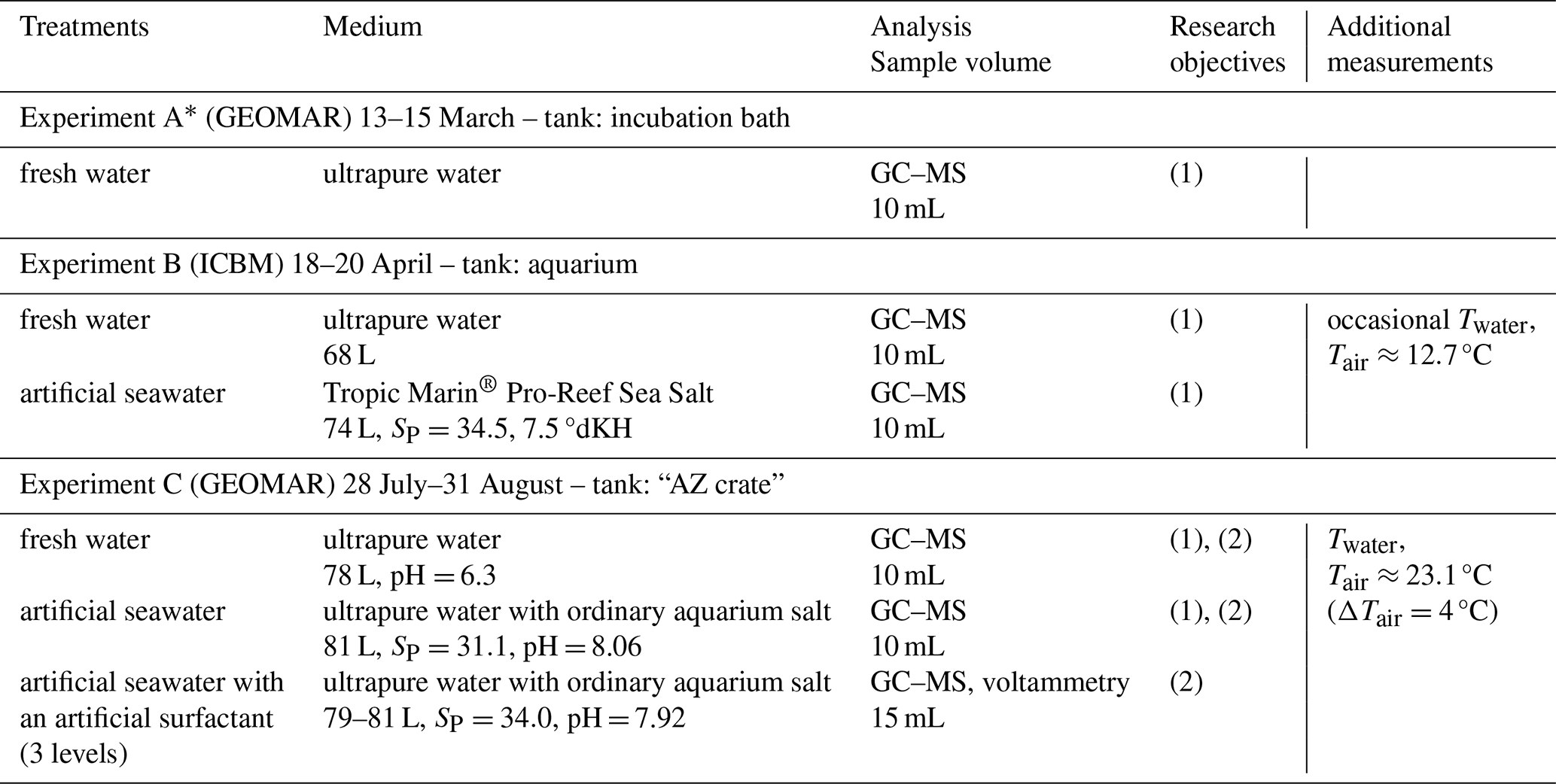
Table 1 summarizes the experiments, which took place in two different locations in Germany: (1) under the roof of the SURF facility at ICBM, Wilhelmshaven and (2) in the laboratories at GEOMAR Helmholtz Centre for Ocean Research Kiel. Two different tanks were used: (1) aquarium made of glass (2) ”AZ crate” (Polypropylene, Schoeller Allibert, Schwerin, Germany).

Table 1 Overview of experiments performed in this study. Sample volumes are the targeted volumes. Gas chromatography–mass spectrometry is abbreviated as GC–MS. The treatments with artificial seawater were prepared with either of two salts, depending on their availability. Details about composition are only available for the medium with Tropic Marin^® Pro-Reef Sea Salt. Research objectives: (1) pure sampling efficiency (2) effect of surfactants on sampling efficiency. ^* Not addressed further in main text, instead see Sect. S1.

2.2 Sampling

Before each sampling, we mixed the water body carefully for 1 min to homogenize any gradients that had formed towards the air side due to the oversaturation and waited for 2 min for the turbulent motion to subside. We sampled the SML, ULW (10–13 cm) and surface (1–6.5 cm). All samples were collected in amber borosilicate glass bottles (20 mL). SML samples were taken with the glass plate technique (Harvey and Burzell, 1972). Following the recommendation by Cunliffe and Wurl (2014) and examples from recent studies (e.g., Adenaya et al., 2021), we reduced the speed of extracting the glass plate to 5 cm s⁻¹. The glass plate (borosilicate glass, 30 cm × 25 cm × 0.5 cm in experiment B, 40 cm × 30 cm × 0.5 cm in experiment C) was immersed to a depth of about 20 or 25 cm. Both sides of the glass plate were wiped with a regular silicone or rubber wiper and the run-off was collected into a sample bottle with a plastic funnel. A single dip provided between 1.8–4.0 mL of medium when no surfactants were present, and 3.4–6.3 mL when an artificial surfactant was added. To collect sufficient sample volume for analysis, two to five dips were required for analysis with gas chromatography–mass spectrometer (GC–MS) and voltammetry samples. The thickness of the sampled layer is determined by Eq. (1) (Cunliffe and Wurl, 2014).

$$\begin{array}{}\text{(1)}& h_{\mathrm{SML}}\approx h_{\mathrm{sampled}}={\displaystyle \frac{V_{\mathrm{sample}}}{n_{\mathrm{dips}}A}}\end{array}$$

where h_SML is the true thickness of the SML, h_sampled is the thickness that was actually sampled in cm, V_sample is the total volume of the glass plate sample in mL, A is the wetted surface area of the glass plate in cm² and n_dips is the number of dips that were needed to collect V_sample.

Each SML sample is always associated with a reference ULW sample and sometimes with additional ULW or surface samples. All samples taken together after the same mixing event are referred to as a sample set. The reference ULW sample was taken immediately after the first dip of the SML sample was collected, interrupting the SML sampling for less than a minute (overall SML sampling took 90–235 s). All additional ULW or surface samples were taken after the SML sample had been finished (exception from this order is 19 April in experiment B). ULW samples were taken with a pipette (5 and 10 mL, Eppendorf SE, Hamburg, Germany) set to the required sample volume by inserting the tip of the pipette vertically and carefully into the water. For sample volumes of 15 mL, a pipette was immersed twice in the same location. ULW samples were taken from a water depth below surface of ∼10 cm in experiment B and ∼13 cm in experiment C. Surface samples were sampled the same way as ULW samples, with the only difference that we were aiming for a depth below surface of less than 1 cm in experiment B and ∼4.5 cm in experiment C (with exception of 31 August: ∼6.5 cm). Additional ULW and surface samples were collected once or twice daily to confirm that the tank was well mixed. These tests were necessary, as the concentration difference between the oversaturated water and the near-zero air is large and might re-establish gradients in the SML quickly. Before each sample set was obtained, all of the equipment was rinsed with ultrapure water.

Samples were taken for trace gas analysis and voltammetry (surfactants). Trace gases were analysed during all of the experiments, whereas voltammetry was only performed in selected cases (Table 1). The targeted sample volume for trace gas analysis was 10 mL. SML samples were filled to at least the targeted sample volume and later on weighed to calculate the sample volume based on the density of the medium. In the treatment with surfactants, a larger sample volume was required for voltammetry measurements to permit a subsequent 10 mL subsample. Given the limited SML volume in the tank and the presence of surfactants, collecting two true replicate SML samples was not feasible. Consequently, the target sample volume was increased to 15 mL for GC–MS analysis, and the purged sample from GC–MS analysis was subsequently reused for surfactant analysis. No effect on final concentrations from the GC–MS measurements was found between 10 and 15 mL samples, as gases are stripped completely out of the medium within the purge time. Sample bottles used for the voltammetry measurements were additionally acid-rinsed (10 % HCl) and pre-combusted at 500 °C before sampling.

2.3 Sample analysis trace gases

The system used to measure the trace gases DMS-d3, isoprene-d5, and ¹³CS₂ is a purge and trap GC–MS (Zavarsky et al., 2018). It consists of a self-constructed purge and trap system, a type 7890A GC, and a 5975C MS (Agilent, Waldbronn, Germany). The GC uses a capillary column (Supel-Q-PLOT, 30 m × 0.32 mm, Merck KGaA, Darmstadt, Germany). The MS is equipped with electrical ionisation, a quadrupole mass filter and a triple-axis electron multiplier detector. All three compounds are measured from the same sample. As samples cannot be preserved, no replicates could be taken for GC–MS analysis. Samples were stored at room temperature in the dark and measured within less than one hour after sampling. Samples (both 10 and 15 mL) are purged with helium (99.999 %, Air Liquide, Düsseldorf, Germany) at a flow rate of 80 mL min⁻¹ for 10 min. The sample gas stream is dried with a Nafion^® membrane dryer (Perma Pure, Lakewood, United States) and trapped with liquid nitrogen in a Sulfinert^® stainless steel tube (Restek GmbH, Bad Homburg, Germany). Injection into the GC is semi-automated with a 6-port valve that channels the carrier gas flow through the trap while it is heated with hot water (70–100 °C) to release the sample. The MS is operated in single-ion mode. The raw peak areas (PA_raw) in the spectra were integrated manually with MSD Productivity ChemStation (version E.02.02.1431, Agilent, Waldbronn, Germany). The unit of PA_raw is arbitrary and, therefore, is not used throughout the manuscript. Qualification and quantification of DMS-d3, isoprene-d5, and ¹³CS₂ was done using $m/z$ ratios of 64 and 65, 72 and 73, and 77 and 79, respectively. The limit of detection (LOD, i.e., minimum PA_raw detectable) was defined as 7 times the root mean square error of the baseline noise and was determined for each compound individually from one representative chromatogram for each experiment. This yielded LODs for DMS-d3 of 209 and 90, for isoprene-d5 of 300 and 309, and for ¹³CS₂ of 258 and 181 respectively for experiment B and C. To extract only isotope signals, all PA_raw were corrected for spectral fragmentation, which causes overlap in the mass spectra of natural and isotopically labelled compounds. A calibration was deemed not necessary, as we are only interested in ratios of SML trace gas content over ULW trace gas content, each sampled directly one after another. The calibration usually used with this setup translates PA_raw linearly into concentrations, which means that the ratio of two PA_raw equals the ratio of concentrations, thus the ratio of two PA_raw is sufficient. It takes less than 1 h to measure all samples from one set, therefore also the drift of the GC–MS is negligible for one sample set. By skipping the calibration, the number of measured SML–ULW pairs for each day was increased. Example calibration curves are shown in Sect. S2. Each PA_raw was normalized by the sample volume to allow for comparability, further referred to as PA. Associated uncertainty of GC–MS measurements is 10 %. An additional step in quality control (QC) was added to identify measurements with poor quality. Peaks of mass 91 at retention time ∼8.10 min were integrated for all SML, ULW and surface samples and normalized by sample volume (PA₉₁). Mass 91 is associated with toluene. There is a stable toluene contamination in the purge system, therefore, the variability in PA₉₁ is indicative of poor-quality measurements (see Sect. S3).

2.4 Sample analysis surface activity

Surface activity (SA) of surfactants was measured only for samples when Triton X-100 (TX-100, with molecular weight 625 g mol⁻¹, Merck, Darmstadt, Germany) was added to the tank (experiment C, see Table 1). Of those samples, only a subset was measured, which was a representative ULW triplicate at the beginning and end of the day, as well as each SML (singlets) sample. SA was quantified using phase-sensitive alternating current voltammetry with a hanging mercury drop electrode 797 VA (Computrace, Metrohm, Switzerland), following the method established by Ćosović and Vojvodić (1982, 1998). This electrochemical technique exploits the adsorption behaviour of surfactants at the interface between the mercury electrode and electrolyte, altering the capacitive current (Scholz, 2015). Samples were stored at −20 °C until analysis. Prior to measurement, all samples were brought to room temperature and adjusted to a uniform ionic strength corresponding to a S_P of 35.0 (0.55 mol L⁻¹ NaCl) to ensure comparability across measurements. Depending on the TX-100 concentration added to the tank, measurements were performed with a deposition time ranging between 10–60 s and a voltage sweep between −0.6 and −1.0 V. Additionally, high TX-100 concentration samples required dilution before measuring (dilutions from 0.7–0.97). For evaluation, the initial current response at −0.6 V was used, and the difference in capacity current between sample and blank was calculated with $\mathrm{\Delta }I=I_{\mathrm{blank}}-I_{\mathrm{sample}}$. Three scans were recorded per replicate and the mean of the three scans was used for final analysis. Calibration was performed using TX-100 across a concentration range of 0.01–1.3 mg L⁻¹. Only the linear portion of the response curve was used for quantification. Analytical precision was assessed using daily standards and blanks, yielding an average precision of 6 %, with all values remaining below 10 %.

For each triplicate of ULW surfactants samples the standard error (SE) of mean was calculated with Eq. (2). Only a few representative ULW samples were taken per day and then were averaged over the day. Errors were propagated with Eq. (3) to show the precision of the daily mean accounting for replicate uncertainty.

$$\begin{array}{}\text{(2)}& {\displaystyle }\mathrm{SE}={\displaystyle \frac{\mathrm{SD}}{\sqrt{n}}}\text{(3)}& {\displaystyle }{\mathrm{SE}}_{\mathrm{day}}={\displaystyle \frac{\mathrm{1}}{m}}\sqrt{{\sum }_{i=\mathrm{1}}^m{\mathrm{SE}}_i^{\mathrm{2}}}\end{array}$$

where SE and SE_i are the standard error of the triplicate, SD is standard deviation of the triplicate, n the number of samples per triplicate, SE_day is standard error of the mean of triplicates per day and m is number of triplicates per day.

Spread of triplicate means is calculated as SD of the mean values with Eq. (4).

$$\begin{array}{}\text{(4)}& {\mathrm{SD}}_{\mathrm{day}}=\sqrt{{\displaystyle \frac{\mathrm{1}}{m-\mathrm{1}}}\sum _{i=\mathrm{1}}^m{\left({\stackrel{\mathrm{‾}}{x}}_i-{\stackrel{\mathrm{‾}}{x}}_{\mathrm{day}}\right)}^{\mathrm{2}}}\end{array}$$

where SD_day is standard deviation for the daily mean, m the number of triplicates, ${\stackrel{\mathrm{‾}}{x}}_i$ the mean of the triplicate and ${\stackrel{\mathrm{‾}}{x}}_{\mathrm{day}}$ the daily mean.

2.5 Sampling efficiency

Sampling efficiency is calculated as ratio of trace gas content per volume in the SML over content per volume in ULW (Eq. 5). Units should be a concentration (e.g., mol L⁻¹) or linearly proportional to the resulting concentration (e.g., PA, which is given per millilitre of sample). Sampling efficiency E is given as a dimensionless fraction. The complement of this fraction represents the sampling losses (Eq. 6). Note, that this resembles the EF commonly computed to determine enrichment in the SML in field samples, e.g., EF = $x_{\mathrm{SML}}/x_{\mathrm{ULW}}$, where x is a measured property.

$$\begin{array}{}\text{(5)}& {\displaystyle }E={\displaystyle \frac{{\mathrm{PA}}_{\mathrm{SML}}}{{\mathrm{PA}}_{\mathrm{ULW}}}}\propto {\displaystyle \frac{C_{\mathrm{SML}}}{C_{\mathrm{ULW}}}}\text{(6)}& {\displaystyle }L=\mathrm{1}-E\text{(7)}& {\displaystyle }{C}_{\mathrm{SML},\mathrm{true}}={\displaystyle \frac{C_{\mathrm{SML}}}{E}}\end{array}$$

where E is sampling efficiency (unitless), PA is the peak area per millilitre of sample, C is a concentration in, e.g., mol L⁻¹, taken from the SML or ULW, as indicated by the subscripts and L is the sampling loss.

Sampling efficiency corresponds to the integrated error introduced by sampling with the glass plate, used in Eq. (7) for correction. This is based on a multiplicative error model, where the error (i.e., sampling efficiency) scales linearly with the quantity needing correction (i.e., measured concentration in glass plate samples), without an offset.

2.6 Additional measurements and recorded parameters

In experiment B, air and water temperature were measured occasionally with common thermometers. In experiment C, additional parameters were measured for each sample set. Practical salinity and temperature of the water were measured with a Cond 330i with a TetraCon 325 (WTW, Weilheim, Germany) at a depth of about 2 cm below surface. The pH of water was measured at about 1.5 cm below surface with a digital pH meter PH-100 ATC (Voltcraft, Hirschau, Germany), calibrated every morning with buffer solutions with pH of 7.0 and 4.0 (Scharlab, Barcelona, Spain). Air temperature was measured with a common digital thermometer (about 46 cm above water surface) and a liquid expansion thermometer (about 15 cm above water surface, low precision of ΔT= 0.5 °C). The number of dips, sample volume in mL (or sample weight in gram) and the person who was sampling were recorded in both experiments. In experiment C, the duration of glass plate sampling in seconds was recorded as well.

2.7 Statistical analysis

Data processing, visualization and statistical analysis was performed in Python version 3.11.11 (Python Software Foundation, 2025). The libraries used for data processing and visualization were pandas version 2.3.2 (McKinney, 2010; The pandas development team, 2025), NumPy version 2.3.3 (Harris et al., 2020), seaborn version 0.13.2 (Waskom, 2021) and matplotlib version 3.10.0 (Hunter, 2007; The Matplotlib Development Team, 2024). For statistical analysis, SciPy version 1.16.2 (Virtanen et al., 2020) and statsmodels version 0.14.5 (Seabold and Perktold, 2010) were used. The main function for each statistical calculation is given below. Parameters of the function call are only mentioned if they were changed from default. Observations with missing values were only excluded if the variable concerned was used in the respective statistical analysis. Outliers were included in descriptive statistics and statistical tests, as large variation was expected and removing outliers would potentially remove true values. In boxplots, however, outliers are shown with the common 1.5 times interquartile range (IQR) in order to present all of the data and to highlight the skewedness. Pair-wise differences between means of treatments and experiments for each trace gas were assessed with Welch's t-test (SciPy, ttest_ind(…,equal_var=False)), as for a few cases the heteroscedasticity could not be safely assumed (minimum and maximum variances were off by a factor of more than 3). No multiple testing correction was applied. One-way ANOVA was used to determine if purging of surfactants samples had an effect on the measurements and to identify (categorical) factors (without order) driving well-mixed ratios in Fig. 3 (SciPy, f_oneway()). The null hypothesis was rejected at p<0.05, and statistical significance assumed accordingly. Where applicable, p-value levels of <0.05, <0.01 and <0.001 are indicated by ^*, ${}^{**}$ and ${}^{***}$ respectively. Levene's test was used to assess similarity of variances for treatments and experiments, since sample sizes per group were small (n≤11) and, consequently, non-normality had to be assumed. Linear regression was calculated with ordinary least-squares (SciPy, linregress()) using Eq. (8). Coefficient of determination R² was calculated as squared Pearson correlation coefficient. Exponential fit was fitted using Eq. (9) (SciPy, curve_fit(…,p0=(max(y),0.1,min(y))). Multiple linear regression (MLR, statsmodels, smf.ols(…).fit(cov_type='HC3')) was used to asses which independent variables drive sampling efficiency. Data was standardized using z-scores before applying MLR with ordinary least-squares (Eq. 10).

$$\begin{array}{}\text{(8)}& {\displaystyle }y=mx+y_{\mathrm{0}}\text{(9)}& {\displaystyle }y=a{e}^{bx}+c\end{array}$$

where y is the dependent quantity, x is the independent quantity, m is the slope and y₀ is the intercept at x= 0 of the linear function, a is the amplitude, b is the exponential rate constant, and c is the asymptote of the exponential function.

$$\begin{array}{}\text{(10)}& Y={\mathit{\beta }}_{\mathrm{0}}+{\mathit{\beta }}_{\mathrm{1}}{X}_{\mathrm{1}}+{\mathit{\beta }}_{\mathrm{2}}{X}_{\mathrm{2}}+\mathrm{\dots }+{\mathit{\beta }}_n{X}_n+\mathit{\epsilon }\end{array}$$

where Y is the response variable, β₀ is the intercept, β_i (i≥1) are the coefficients determined by the MLR, X_i are the independent variables and ε is the error term. Reported are R² and adjusted R², which accounts for the number of predictors vs samples size, and p-value for F-statistics. Heteroscedasticity was not assumed.

3 Results

A total of 155 samples were taken (53 SML–ULW pairs), of which 149 samples (51 SML–ULW pairs) satisfied formal QC. An additional 13 samples (5 SML–ULW pairs) were removed, as our experimental assumptions were not satisfied, leaving a total of 46 SML–ULW pairs for sampling efficiency calculations.

The results presented here are based exclusively on experiment B and C, as experiment A were preliminary tests. Furthermore, our assumption that the tank was well-mixed is tested. PA of the trace gases for SML and ULW and their correlation are presented to support the choice of a multiplicative error model (Eq. 7). Final sampling efficiency is shown for water without additives first, and then including an artificial surfactant.

3.1 Experimental conditions and parameters

3.1.1 Water temperature and salinity

The overall water temperature range across all experiments and treatments was 17.2–23.1 °C. Water temperature was similar in both treatments in experiment B. The temperature in the FW treatment was only measured once at the end of the day (16:30 UTC, 19 April), yielding 20.9 °C. Having been filled the previous day and stored under the SURF roof overnight, the water likely warmed over the course of the day, reaching 20.9 °C at the time of measurement. The AS treatment on the next day started off warmer and cooled down over the course of the day, averaging to 21.5 °C (ΔT= 4.6 °C). In experiment C (located in lab), a larger range of water temperatures was targeted by using refrigerated water that would heat up in the course of the day to room temperature. This was only partially successful, as the targeted water temperature of < 10 °C to start with was not achieved. The FW treatment averaged at 17.6 °C, AS at 19.5 °C and the treatment with artificial surfactants at 20.6 °C (with ΔT of 1.2, 3.0 and 1.5 °C respectively). Water temperature of FW treatment overlaps partially with the AS treatment, and the AS treatment partially with the treatment including surfactants, allowing for continuity across treatments.

Salinity was set to either zero or to oceanic levels. S_P was between 28.9 and 34.6 in all treatments with salt amendments. Salinity was kept constant for each treatment level (FW, AS, and each of the SA levels), with exception of the AS treatment without surfactants, which combines two lab days. On 8 August the targeted practical salinity of 34.5 was not reached, but 29.0±0.07. This was corrected to 34.6 on 10 August 2023.

3.1.2 Surface activity and enrichment of surfactants

An artificial surfactant was added in experiment C to AS only. Since GC–MS samples were reused for voltammetry analysis, it was tested, if the delayed freezing and the purging had an effect on measured SA. Comparison was performed on a specially collected sample set (n= 6) and across all ULW samples with voltammetry measurements (n= 36). Neither purging (one-way ANOVA failed to reject null hypothesis, p_all= 0.8864 with n= 36, p_subset= 0.5138 with n= 6) nor the delayed freezing (one-way ANOVA failed to reject null hypothesis, p_all= 0.3788 with n= 30) had a significant effect. SA of purged and non-purged samples is thus treated the same (data points shown in Fig. S5).

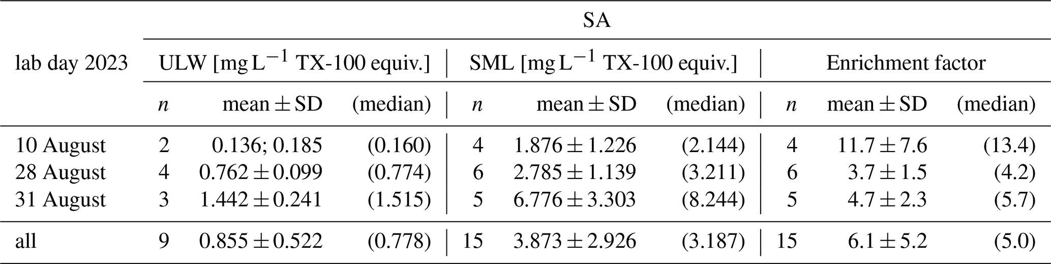
The goal was for the surfactants to reach EF = 1 after wet surfactant TX-100 was added to AS. We targeted a range of SA, so on each day a different amount was added to the tank, increasing over time (Table 2). Mean SA_ULW ranged from 0.160 to 1.515 mg L⁻¹ TX-100 equiv., while mean SA_SML was much higher between 2.144 to 8.244 mg L⁻¹ TX-100 equiv., consequently the SML was always enriched with three exceptions where EF < 1.0, once for each level of TX-100 added. Exceptions could neither be explained with sample sequence (i.e., first sample of day or after a long break), how often the tank had been mixed before already, (absolute) SA, amount of TX-100 added, age of the water (i.e., time since filling), contamination from sampling equipment, water temperature, salinity, nor by reported deviations from standard procedure in sampling protocols (e.g., person sampling, mixing times, unexpected events), in GC-MS measurement protocols (because each SML sample was first measured for trace gas content), or in voltammetry measurement protocols (e.g., handling errors, failures). Exceptions were, therefore, not excluded, yielding an average EF from 3.7–11.7. SA_ULW was usually pretty consistent for one added amount of TX-100 (standard deviation < 0.241 mg L⁻¹ TX-100 equiv.), whereas SA_SML varied much more with standard deviations from 1.226 to 3.303 mg L⁻¹ TX-100 equiv., which in turn resulted in high standard deviation in the EF as well.

Table 2 Surface activity (SA) measurements and corresponding enrichment factors (EF) in experiment C per day in the laboratory in treatment artificial seawater (AS) with surfactants. Each day a different amount of TX-100 was added, increasing over time. For n= 2 minimum and maximum values are depicted instead of mean and standard deviation.

3.1.3 Sampling duration, sample volume and number of dips

The duration of sampling was recorded for SML samples from right before the first dip until the vial was closed with the rubber stopper as a potential driver for sampling efficiency variability. Sampling duration ranged from 54–235 s over all experiments. Only a few durations were recorded in experiment B in the AS treatment, amounting to 135 s on average. In experiment C, the shortest sampling duration was recorded for the AS treatment with a mean of 112 s. FW sampling took longer with 145 s on average. While the SA was increased each day, the sampling duration decreased from 183 s initially (10 August), to 139 s on the second day (28 August) and 129 s on the last day (31 August). Sampling duration greatly depends on the number of dips, which in turn depends on the targeted sample volume. Sampling the treatment with surfactants overall took longer to sample than the AS treatment, because 15 mL were targeted instead of 10 mL.

ULW samples were taken with a pipette, resulting in exact sample volumes of 10 and 15 mL respectively. SML samples, on the other hand, showed variation depending on how much water would stick to the glass plate per dip. FW and AS samples were mostly slightly larger than the targeted 10 mL (10.8 ± 1.0, n= 30). The samples with the lowest TX-100 added were mostly slightly less than the targeted 15 mL (14.3 ± 0.7, n= 4). For the next increase of TX-100, sample volumes were mostly slightly more than the targeted 15 mL (15.9 ± 1.0, n= 6). For the highest concentration of TX-100, all samples were below the targeted 15 mL (12.5 ± 1.3, n= 6). This is linked to how much sample volume can be gathered per dip (Figs. 1, 2). In the treatment with the highest TX-100 concentration, another (full) dip would have resulted in too much volume for GC–MS analysis (i.e., not enough headspace). Note, that on 28 August (medium concentration of TX-100) also half dips were captured (n= 2), i.e., only the wipe of the first side of the glass plate was filled into the vial. The second side was discarded.

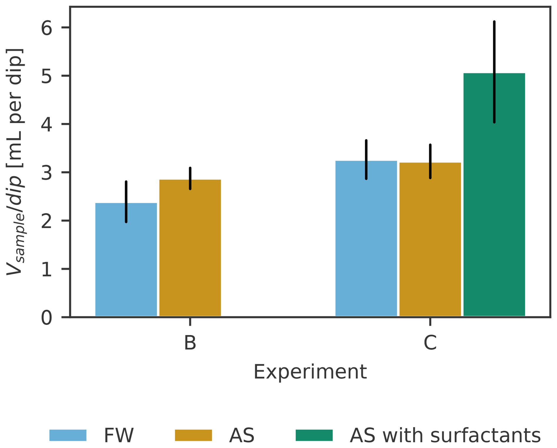
Figure 1 Collected sample volume V_sample for SML samples per dip of the glass plate in the three treatments. Black lines indicate standard deviation.

Figure 2 Sample volume collected per dip against SA in experiment C.

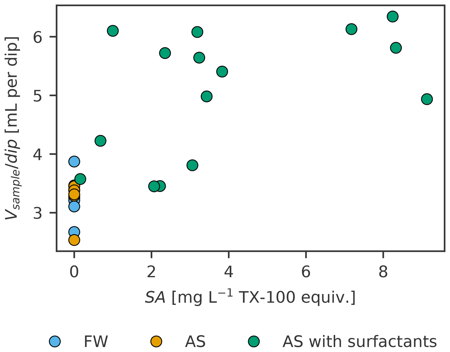
The number of dips was recorded to calculate the operational SML thickness (Eq. 1) and as a potential, additional source of sampling efficiency variability besides sampling duration. To fill about 10 mL of sample without artificial surfactants, three to five dips were required, whereas two to four dips were required to fill about 15 mL with artificial surfactants added (Fig. 1). FW and AS are similar, also across experiments (FW and AS in experiment B 2.4 and 2.9 mL per dip, in experiment C 3.3 and 3.2 mL per dip respectively). In the treatment with an artificial surfactant, significantly more volume (5.1 mL per dip) was collected per dip, on average, while the volume collected per dip increases with the amount of TX-100 present in the SML (measured as SA), as shown in Fig. 2.

An increased sample volume per dip indicates that a thicker layer was sampled (Eq. 1). Layer thickness ranged from 25–63 µm. In experiment B, FW and AS differ at 40 ± 7 and 48 ± 4 µm, while the sampled layer was thinner and more similar in FW and AS in experiment C, with 33 ± 4 and 32 ± 3 µm respectively. In the treatment with an artificial surfactant, the thickness increased to an average of 51 ± 10 µm.

3.2 Mixing in the tank

Our experiments are based on the premise that SML and ULW have the same trace gas concentration, achieved by mixing the tank before each sampling. In order to test our assumption, a reference ULW sample (PA_ref) was taken and compared to samples from other depths and locations in the tank (Fig. 3). PA was either taken at reference depth, but at a different location, or at the surface. Almost all ratios (PA $/$ PA_ref) lie within the range of uncertainty of the measurements (grey shaded area) for all three trace gases. Four sample sets outside that range (i.e., not well mixed, indicated as grey points) were removed manually from further calculations (i.e., sampling efficiency), as the additional QC did not indicate poor quality, nor were there deviations from the general sampling procedure noted in the protocols. Four points for isoprene-d5 and three for ¹³CS₂ from 20 April and 8 August were outside the uncertainty range, but were not removed from the data set. Mean values of the ratios (excluding grey points) are 1.00 ± 0.05, 1.01 ± 0.10, and 1.01 ± 0.08 for DMS-d3, isoprene-d5, and ¹³CS₂ respectively. Standard deviations vary between trace gases, with the largest variation for isoprene-d5. Ratios are independent of sampling location, depths, day or experiment (one-way ANOVA failed to reject null hypothesis in all cases).

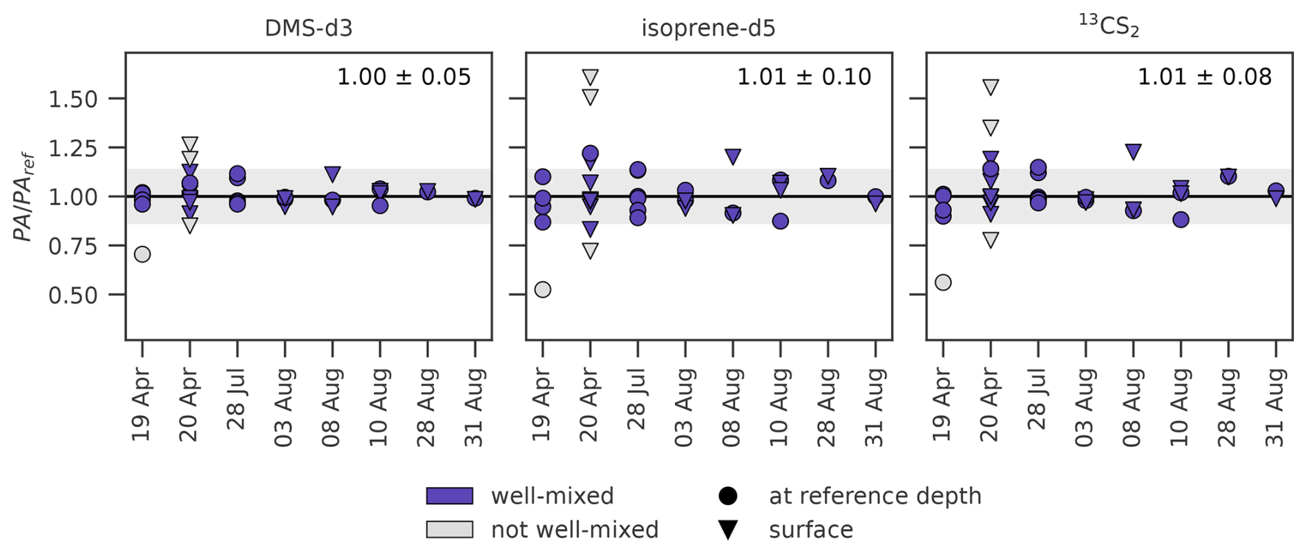
Figure 3 Test for uniform trace gas concentration in the tanks (well-mixed). The ratios PA $/$ PA_ref (n= 37) are shown against date for DMS-d3 (left), isoprene-d5 (middle) and ¹³CS₂ (right). Black horizontal line depicts PA = PA_ref (i.e., well-mixed). Grey shaded area indicates ± 14.1 % uncertainty, calculated by error propagation. Grey points (n= 4) were identified as not well-mixed. Mean and standard deviation for PA $/$ PA_ref is indicated in upper right of each subplot (excluding grey points). April samplings belong to experiment B, all other samplings are experiment C. All three treatments (FW, AS, AS with surfactants) are included.

3.3 Trace gas abundances

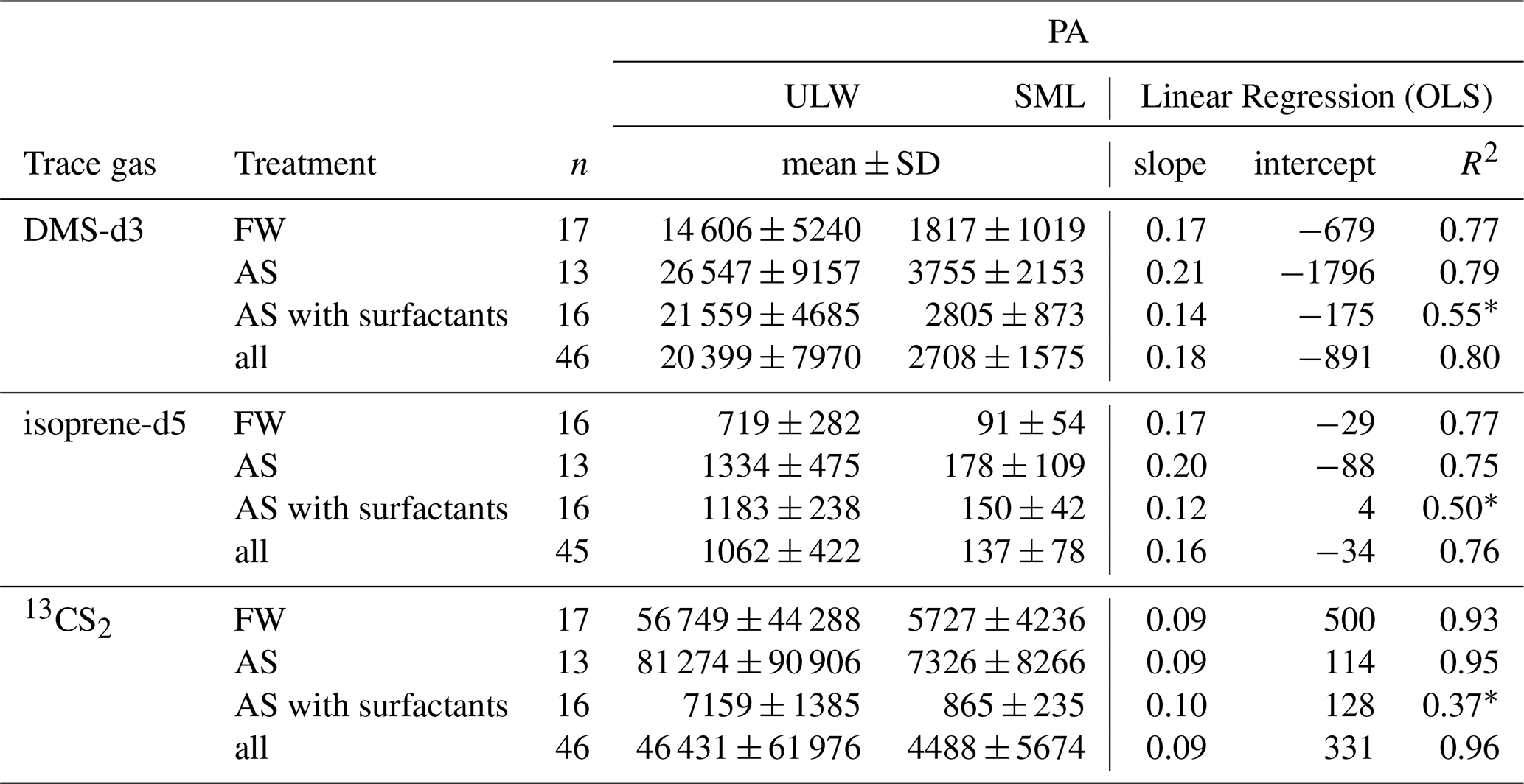
Figure 4 shows measured PA from treatments FW, AS and AS with surfactants, plotted as SML against ULW, for DMS-d3, isoprene-d5, and ¹³CS₂. The SML value is always much lower than the ULW value. The order of magnitude for PA varies between trace gases due to different amounts of trace gas in the spike and different trapping and ionisation efficiencies. Therefore, while comparisons of PA within the same trace gas are valid, direct intercomparisons across trace gases are not possible due to the skipped calibration. DMS-d3 is in the order of 10⁴, isoprene-d5 at 10³, and ¹³CS₂ up to 10⁵. ¹³CS₂ shows two distinct clusters of points, as the two spikes used were significantly different in the amount of ¹³CS₂, whereas the amounts for DMS-d3 and isoprene-d5 were similar. For all three gases, a clear linear, positive correlation is visible between SML and ULW. R² of the linear fit (SciPy, linregress()) for DMS-d3 and isoprene-d5 are both 0.77 for FW, 0.79 and 0.75 for AS, and much lower at 0.55 and 0.50 for AS with surfactants respectively. R² for ¹³CS₂ is 0.93 for FW and 0.95 for AS, and much lower than for the other trace gases for AS with surfactants at 0.37. Note, that the latter data points all fall exclusively into one cluster only, indicating a bad fit without the influence of the large spread present for FW and AS. These values, together with slope and intercept as well as mean PA with standard deviation are reported in Table 3. Mean values and standard deviation visualize the order of magnitude, as within each treatment the amount of spike added differed slightly, causing high standard deviation. This is especially visible for ¹³CS₂, where standard deviation is close to the mean value for FW and AS (includes both clusters), but standard deviation is much lower than the mean for AS with surfactants (only lower value cluster). Slopes differ slightly between gases and treatments. Slopes for DMS-d3 are 0.17 (FW), 0.21 (AS) and 0.14 (AS with surfactants). Slopes for isoprene-d5 are similar, with 0.17 (FW), 0.20 (AS) and 0.12 (AS with surfactants). Slopes for ¹³CS₂ are lower, with 0.09 (FW and AS) and 0.10 (AS with surfactants). Intercepts are not zero, but all are much smaller than the respective mean PA_ULW and therefore considered negligible. Correlation of all data points without distinguishing treatments yields R² of 0.80 (DMS-d3), 0.76 (isoprene-d5) and 0.96 (¹³CS₂).

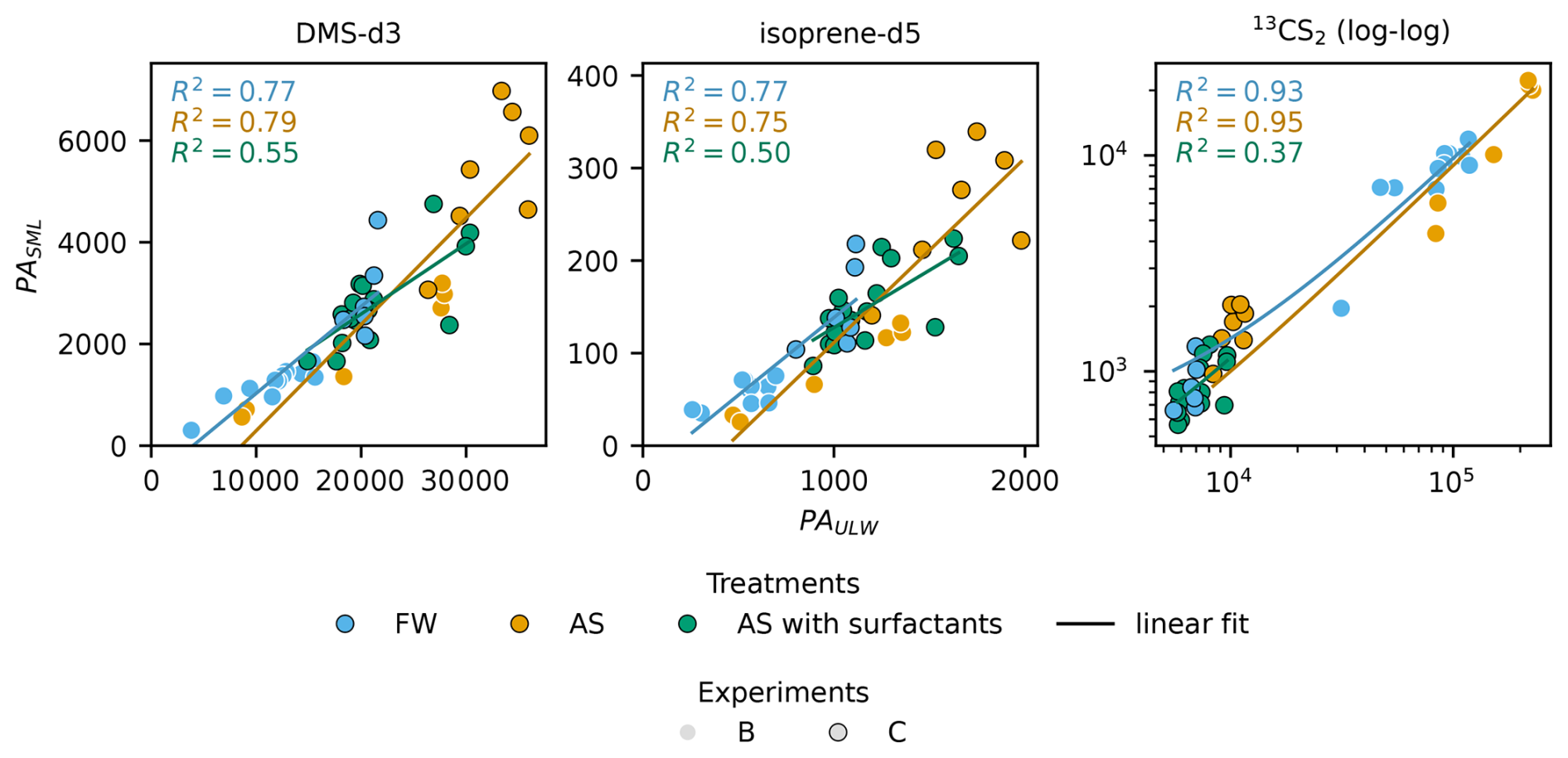
Figure 4 Correlation of SML and ULW PA for DMS-d3 (left), isoprene-d5 (middle) and ¹³CS₂ (right), grouped by treatments fresh water (FW) and artificial seawater (AS) without and with surfactants. Linear fits for ¹³CS₂ were performed on the non-logged data, log-log scale is only used to better visualize the very low values.

Table 3 Linear regression of PA of SML and ULW samples for DMS-d3, isoprene-d5, and ¹³CS₂. All R² show a strong fit, except when marked with ^* (moderate fit).

3.4 Sampling efficiency for fresh water and artificial seawater

The sampling efficiency of the trace gases is calculated using the ratio of measured PA in SML over measured PA in ULW (Eq. 5). Due to mixing in the tank the theoretical maximum value for the sampling efficiency is, thus, 1.0 (or 100 %), i.e., when PA_SML= PA_ULW.

Figure 5 shows sampling efficiency for the studied trace gases in FW and AS treatment, separated by experiment. Overall the three trace gases exhibit similar trends in E, but there are significant differences between the experiments (fails to reject null hypothesis with p < 0.001, Table 5). In experiment B sampling efficiency is lower than in C. For all three trace gases, sampling efficiency decreases in experiment B with the addition of salt, whereas, this reverses for experiment C and sampling efficiency increases with the addition of salt.

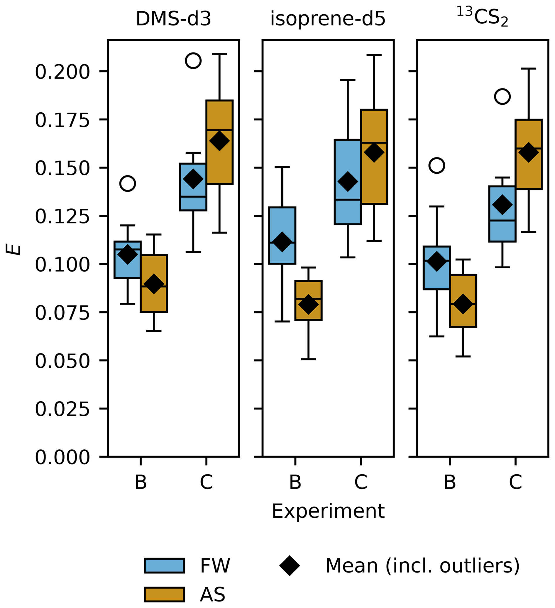
Figure 5 Sampling efficiency (E) for DMS-d3 (left), isoprene-d5 (middle) and ¹³CS₂ (right), separated by experiment, coloured by treatments fresh water (FW, blue) and artificial seawater (AS, orange). Box width shows 25 to 75 percentile, centre line denotes the median, diamonds denote the mean, open circles denote outliers, and whiskers show minimum and maximum. The number of data points in experiment B is n_FW= 11 (n_FW= 10 for isoprene-d5) and n_AS= 6, in experiment C n_FW= 6 and n_AS= 7.

Mean sampling efficiency for DMS-d3 in experiment B is 0.105 ± 0.018 (n= 11) in FW, decreasing to 0.090 ± 0.020 (n= 6) in AS, though the difference is not significant (p= 0.15, outliers in Fig. 5 included). In experiment C, the mean sampling efficiency for DMS-d3 in both treatments is higher than in experiment B, with 0.144 ± 0.034 (n= 6) in FW increasing to 0.164 ± 0.033 (n= 7) in AS. The difference between FW and AS within experiment C is not significant (p= 0.32). This overall picture repeats for isoprene-d5 and ¹³CS₂. In experiment B, mean sampling efficiency for isoprene-d5 is 0.112 ± 0.025 (n= 10) in FW, reducing to 0.079 ± 0.018 (n= 6) in AS, whereas in experiment C sampling efficiency is overall higher, with 0.143 ± 0.035 (n= 6) in FW and then further increasing to 0.158 ± 0.036 (n= 7) in AS. For ¹³CS₂, sampling efficiency in experiment B averages to 0.101 ± 0.025 (n= 11) in FW and lowers to 0.079 ± 0.019 (n= 6) in AS, whereas it is overall higher in experiment C with 0.131 ± 0.032 (n= 6) in FW and rising to 0.158 ± 0.031 (n= 7) in AS. Similar to DMS-d3, the differences within both experiments between treatments are not significant (Table 5), except for isoprene-d5 in experiment B (p= 0.009).

Standard deviations of sampling efficiency are slightly larger in experiment C than in B for all three trace gases and differ significantly between treatments FW and AS (Levene's test for equal variances failed to reject null hypothesis with p 0.045, 0.0497 and 0.033 for DMS-d3, isoprene-d5, and ¹³CS₂, SciPy, levene(…,centre='mean')). Standard errors are almost two times larger in experiment C than in B. Standard error (SE) in FW and AS for DMS-d3 is 0.0074 and 0.013, for isoprene-d5 is 0.0080 and 0.014 and for ¹³CS₂ is 0.0073 and 0.013. SE overall (n= 30) are 0.0070, 0.0074 and 0.007 for DMS-d3, isoprene-d5, and ¹³CS₂.

There is no significant difference between FW in experiment B and C for any of the three trace gases (except for DMS-d3, p= 0.038), but in AS the differences are significant for all three trace gases (p < 0.001), see Table 5. The medium used in FW was ultrapure water, from different devices, but same models. The media used for AS, on the other hand, were different in the composition of the salts and other substances added, though also S_P slightly varied.

Sampling efficiency as a function of water temperature, salinity, spike volume per litre added (i.e., proportional to trace gas concentration) and number of dips was investigated using MLR models (n= 19 complete observations of 30). Note, that 10 of 11 data points in experiment B treatment FW were excluded, because of missing temperature measurements, and one of seven in experiment C treatment AS, because of unrecorded number of dips. The MLR models were significant for all three trace gases (F(4,14) > 5.6, p < 0.01) and explain about 60 % of the variance observed in sampling efficiency (adjusted R² is 0.63, 0.60 and 0.65 for DMS-d3, isoprene-d5, and ¹³CS₂ respectively). The models predicted average (±SE) sampling efficiency of 0.129 ± 0.007, 0.127 ± 0.008 and 0.120 ± 0.007 for DMS-d3, isoprene-d5, and ¹³CS₂, when all predictors were at their mean values (p < 0.001). Spike volume per litre is a significant, positive predictor for sampling efficiency for all three trace gases (p < 0.01, β is 0.0342, 0.0404 and 0.0353 for DMS-d3, isoprene-d5, and ¹³CS₂, s_spike= 1.4 µL L⁻¹). For DMS-d3 and ¹³CS₂ also water temperature is a significant, but negative predictor (p < 0.05, β is −0.0223 and −0.0219, s_Tw= 1.8 °C), whereas, for isoprene-d5 the number of dips is a significant, positive predictor (p= 0.018, β= 0.0213, s_dips= 0.6). Salinity was not a significant predictor for any of the trace gases (p between 0.448 and 0.608). See Sect. S5 for details of MLR, linear regression results and additional plots.

3.5 Sampling efficiency with an artificial surfactant

Since surfactants are often present in natural surface waters, the experiments were extended to include a treatment of AS with surfactants.

When an artificial surfactant (TX-100) was added to AS (Fig. 6), the mean sampling efficiency for all of the three trace gases reduced even below the FW treatment, DMS-d3 to 0.130, isoprene-d5 to 0.127 and ¹³CS₂ to 0.121 (Table 4). Standard deviations are also smaller than in FW and AS treatment (0.025 for DMS-d3, 0.024 for isoprene-d5 and ¹³CS₂). The range (difference from minimum to maximum) is still similar to the range observed in FW and AS for each of the three trace gases.

Table 4 Summary statistics of sampling efficiency for DMS-d3, isoprene-d5, and ¹³CS₂ in experiment B and C in fresh water (FW) and artificial seawater (AS) without and with surfactants treatment, as visualized in Figs. 5 and 6. ^* indicates in which group one data point had to be removed for isoprene-d5 (PA_SML < LOD).

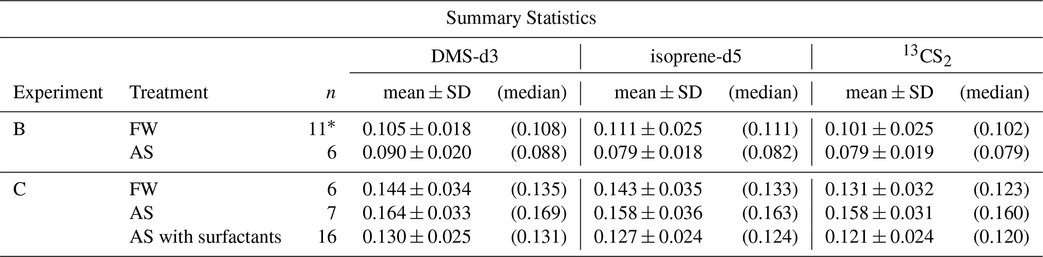
Table 5 Test statistics of sampling efficiency for DMS-d3, isoprene-d5, and ¹³CS₂ in experiment B and C in fresh water (FW) and artificial seawater (AS) treatment, as visualized in Fig. 5. ¹ indicates in which group one data point had to be removed for isoprene-d5 (PA_SML < LOD). ^*, ${}^{**}$ and ${}^{***}$ mark where the null hypothesis was rejected, with p-values < 0.05, < 0.01 and < 0.001 respectively.

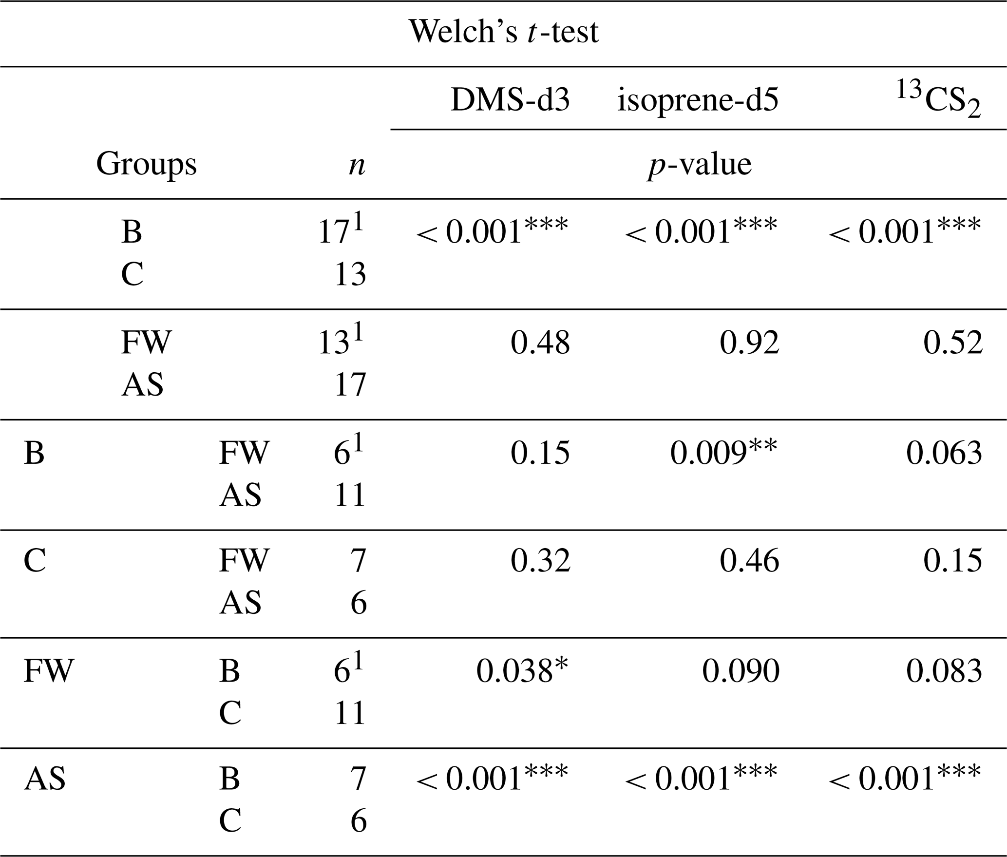
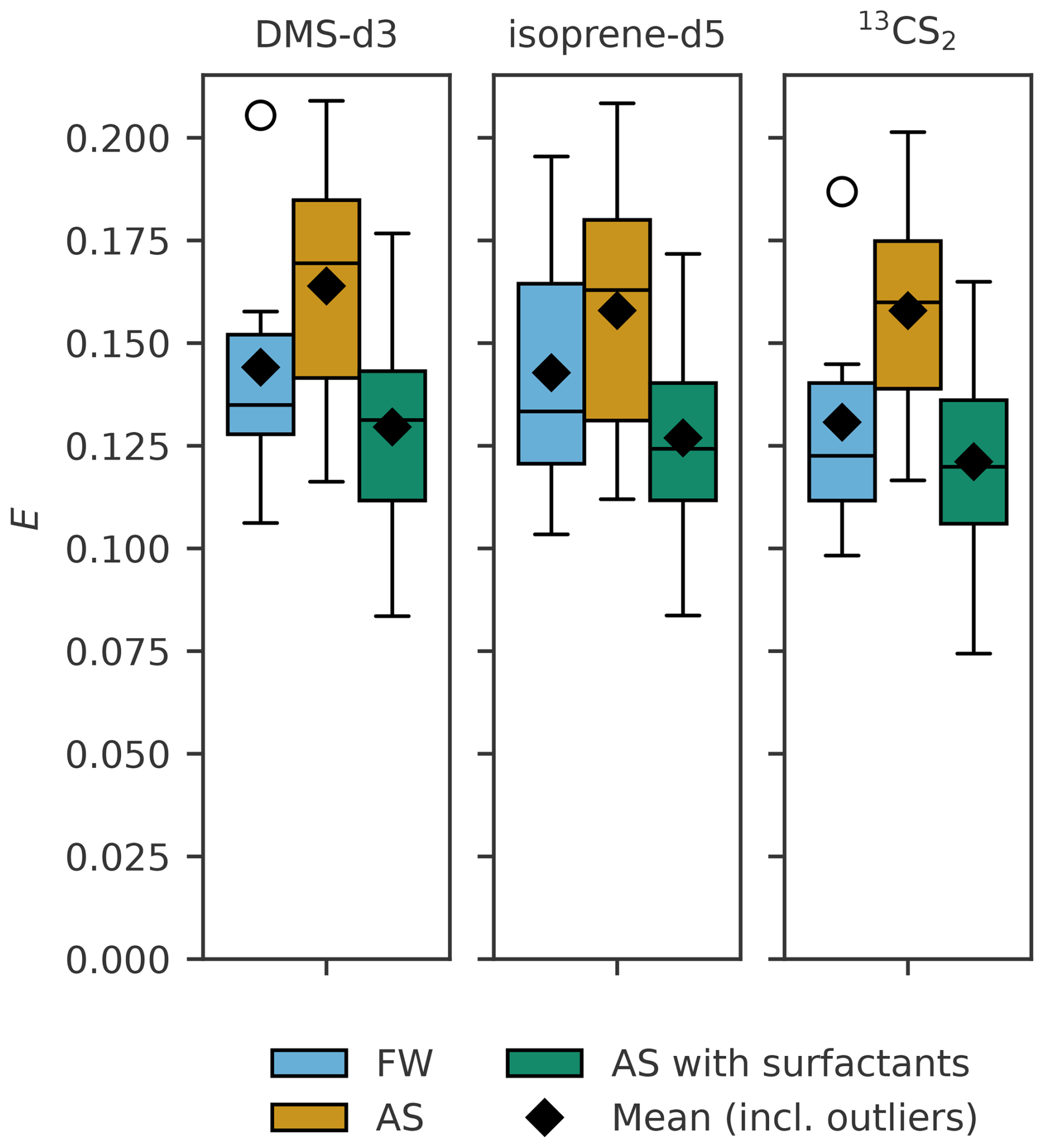
Figure 6 Sampling efficiency (E) for DMS-d3 (left), isoprene-d5 (middle) and ¹³CS₂ (right) when artificial surfactants are added to artificial seawater (AS with surfactants) from experiment C (S_P= 31.1±2.9). Fresh water (FW) and artificial seawater without surfactants (AS) are depicted as well for reference. Box width shows 25 to 75 percentile, centre line denotes the median, diamonds denote the mean, open circles denote outliers, and whiskers show minimum and maximum. The number of data points is n_FW= 6, n_AS= 7 and n_SA= 16.

Sampling efficiency decreases with increasing SA_SML (Fig. 7). It decreases fast from SA = 0 until about SA = 3.0. Above SA = 3.0 the values seem to arrange around a constant value of sampling efficiency. Linear fit is weak (R² between 0.26 and 0.28 for all three trace gases). The slope is negative and small with about −0.005 per mg L⁻¹ TX-100 equiv. and intercepts are between 0.146 to 0.154 for the three trace gases (Table 6). Though small, the slope is significantly different from no slope (p < 0.05 for all three trace gases). An exponential fit was only possible for DMS-d3 and ¹³CS₂, for which it explains slightly more variability than the linear fit (R² between 0.42 and 0.44). When treatment FW was included an exponential fit was only possible for DMS-d3 (not shown). The exponential fit approaches 0.12 and 0.11 for DMS-d3 and ¹³CS₂ with a small amplitude of 0.05 for both at a decay rate of −0.68 and −0.88. The exponential fit is added for visualization in Fig. 7.

Table 6 Curve fitting for sampling efficiency (E) against SA_SML in experiment C, treatments with AS only. ^* marks where the null hypothesis was rejected, with p-value < 0.05.

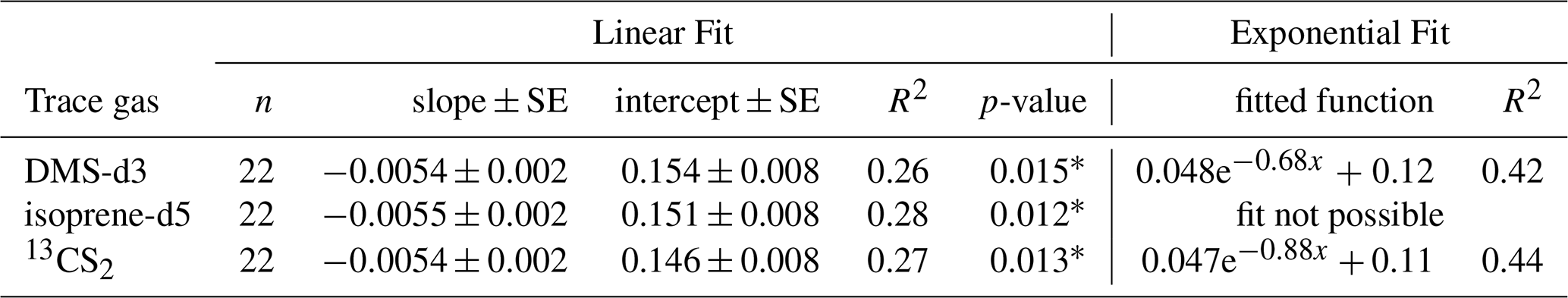
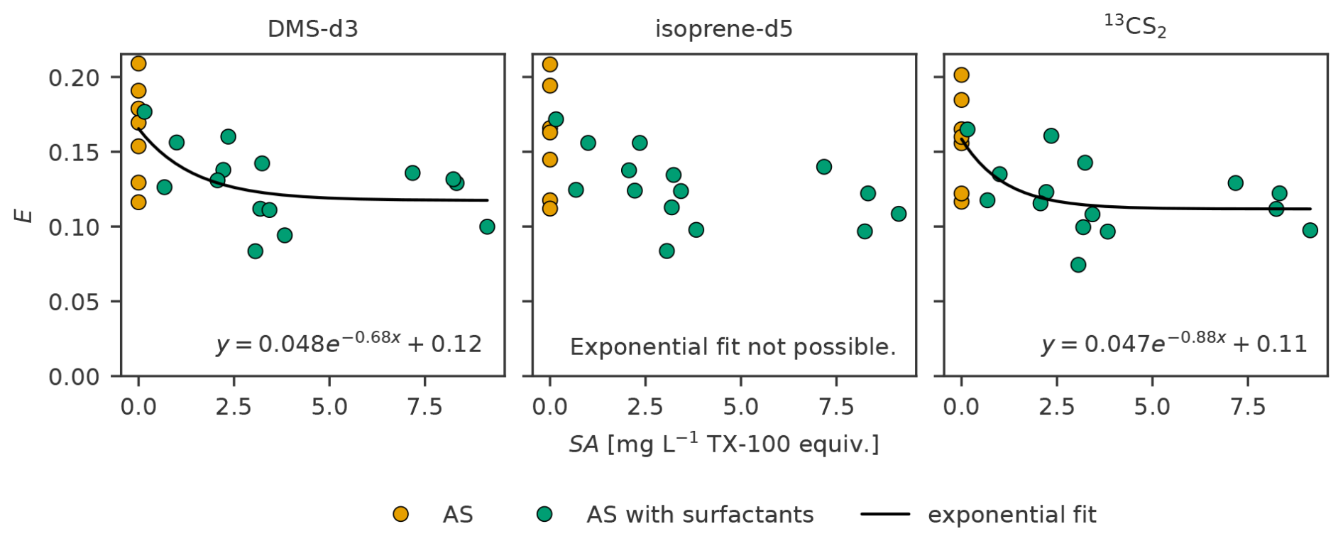
Figure 7 Sampling efficiency for DMS-d3 (left), isoprene-d5 (middle) and ¹³CS₂ (right) against surface activity (SA) in experiment C. Exponential fit is added as aid for visualization.

Sampling efficiency in response to water temperature, salinity, spike volume per litre added (i.e., proportional to trace gas concentration), number of dips and SA in the SML was investigated using MLR models for each trace gas (n= 27 complete observations of 29). The MLR models were not significant for any of the three trace gases (F(5,21) > 1.9, p > 0.09) and explained less than 25 % of the variance observed in sampling efficiency (adjusted R² is 0.25, 0.22 and 0.23 for DMS-d3, isoprene-d5, and ¹³CS₂ respectively). The model predicted average (±SE) sampling efficiency of 0.139 ± 0.006, 0.137 ± 0.006 and 0.131 ± 0.006 for DMS-d3, isoprene-d5, and ¹³CS₂, when all predictors were at their mean values (p < 0.001). Spike volume per litre is a significant, positive predictor for sampling efficiency only for DMS-d3 (p= 0.029, β = 0.0213, s_spike= 0.94 µL L⁻¹). Water temperature is a significant, negative predictor for all three trace gases (p < 0.05, β is −0.0324, −0.0309 and −0.0321 for DMS-d3, isoprene-d5, and ¹³CS₂, s_Tw= 1.4 °C). SA in the SML was a significant, negative predictor for ¹³CS₂ only (p= 0.041, β= −0.0137, $s_{\mathrm{SA},\mathrm{SML}}=$ 2.91 mg L⁻¹ TX-100 equiv.), though DMS-d3 is on the limit (p= 0.05), and isoprene-d5 is non-significant (p= 0.07). Neither number of dips (p > 0.8), nor salinity (p is 0.247 and 0.206 for DMS-d3 and isoprene-d5, but much lower at 0.066 for ¹³CS₂) were a significant predictor for any of the trace gases. See Sect. S6 for details of MLR, linear regression results and additional plots.

4 Discussion

4.1 Experimental setup

Water temperature in this study covered a modest range of ΔT= 5.9 °C. Sea surface temperature in the field encompasses a wider range. At the time-series station Boknis Eck (Western Baltic Sea), for example, the range studied here is only observed during the summer season (Laß et al., 2013). In our treatments, intermediate salinity was excluded, focussing on fresh water and seawater. We do not expect to see any improvement in our results by including intermediate salinity, as salinity was a non-significant predictor for sampling efficiency. Additionally, we did not expect that the type of salt (Tropic Marin^® Pro-Reef Sea Salt vs. ordinary aquarium salt) would have an effect. Differences in the FW treatments between experiments were not statistically significant, while for the AS treatment they were (Table 5). We do not attribute this to the composition of the salt (affecting the solubility differently than ordinary aquarium salt, e.g., Weisenberger and Schumpe (1996)), other substances, or the alkalinity of the water (see Table 1 for details of the salts), as neither are known to affect the isotopically labelled trace gases used in this study. Additionally, they are not expected to alter the physicochemical properties enough to affect sampling efficiency as they are dosed in natural concentrations. As the three trace gases exhibit a similar effect, something more general appeared to change between the AS experiments. It is, therefore, more likely that the differences are attributable to the combined effect of changes in (environmental) parameters between experiments, which were not ideally overlapping across all treatments (see Fig. S6), e.g., changes in number of dips, water temperature, different glass plate size and wiper, mixing in of the trace gases, degree of oversaturation. In that respect, the differences between B and C might also be explained by a smoother sampling routine in C due to the practice gained in B.

The increase in targeted sample volume from 10 mL (FW, AS) to 15 mL (AS with surfactants) did not affect PA_ULW. However, we could not assess whether PA_SML differed between 10 and 15 mL. The increase in volume is achieved by dipping the glass plate more often, potentially affecting the sampling efficiency. Since the number of dips was a non-significant predictor for sampling efficiency in the MLR, the effect on PA_SML and consequently on sampling efficiency, is considered negligible. Finally, a range of saturation states was not investigated. We only performed experiments with oversaturated conditions in the water, but we expect that the concentration gradient (magnitude and direction) has an effect on sampling efficiency.

Each experiment was conducted at a different location (and time of year, Table 1). The tanks were placed indoors (the roof at ICBM in experiment B closes all around), to make sure that results are independent of location (and time of year), and consequently comparable between experiments. Air properties (e.g., temperature, humidity) likely varied (though not measured), but due to the strong concentration gradient we deem their effect negligible. The material of the tanks was either glass or plastic (Table 1). Contamination was ruled out, since we were using isotopically labelled trace gases. Neither of the materials used is known to react with the studied isotopically labelled trace gases or the added artificial surfactant. Adsorption to the surfaces likely differs between glass and plastic, as well as the exchange of heat across the material. These effects are accounted for by measuring water temperature and surface activity.

The above noted differences in setup between experiment B and C make the interpretation of our results more difficult, given that no clear factor driving the differences between the experiments could be identified. The effect of the differences does not seem to overrule the overall trends (as seen in the combined data set of B and C in Fig. S6). Throughout this manuscript we kept information about the source experiment visible (except for Table 7).

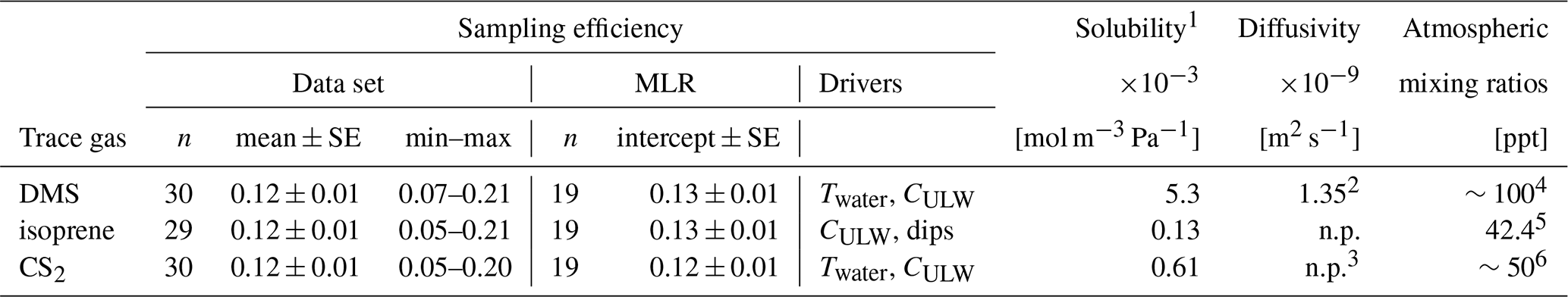
Table 7 Sampling efficiency summarized from treatment FW and AS. Treatment with an artificial surfactant is omitted here, since it remains uncertain whether our premise (well-mixed) was met. All trace gases were oversaturated. Isotopically labelled trace gases were used as analogues for the gases listed here. MLR is multiple linear regression, T_water is the water temperature and C_ULW the concentration of trace gas in the ULW. ¹ Values copied from solubility compilation by Sander (2023). ² Value calculated for T= 25 °C and S_P= 0 from Saltzman et al. (1993). Diffusivity in (sea)water is not published (n.p.) for isoprene or CS₂. ³ Due to their analogous structures, CO₂ diffusivity can be used as an approximation for CS₂, i.e., $D_{{\mathrm{CO}}_{\mathrm{2}}}=$ 1.88 × 10⁻⁹ m² s⁻¹ at T= 25 °C and S_P= 0 (Mazarei and Sandall, 1980). Global estimates of atmospheric mixing ratios are taken from ⁴ Liss et al. (2014), ⁵ Ferracci et al. (2024), Southern Ocean only, and ⁶ Lennartz et al. (2020).

4.1.1 Mixing in the tank

Figure 3 shows that the tank was well-mixed on all days, because almost all the ratios PA $/$ PA_ref are within the acceptable uncertainty range. The four points from 20 April and 8 August, which were not acceptable for isoprene-d5, and the three for ¹³CS₂, are still considered as well-mixed, since the ratios are acceptable for DMS-d3. The mean values of the ratios (excluding grey points) are all close to 1.0 (i.e., PA = PA_ref), supporting that the tank was well-mixed without any physically driven gradients present or forming, as then the mean would likely show an offset. This is further supported by the ratios with surface samples on 20 April, sampled as close as possible to the surface. Due to the oversaturation in the tank and near-zero atmosphere, we hypothesize that PA_surface < PA_ULW should develop as result of the outgassing, causing ratios with surface samples to systematically drop below 1.0. However, in Fig. 3 they distribute equally around 1.0. The increased standard deviation of isoprene-d5 as compared to the other two trace gases, can be attributed to increasing integration error as raw, non-normalized PA of isoprene-d5 were generally close to the LOD, whereas, DMS-d3 and ¹³CS₂ were usually sufficiently above the LOD for the integration error to diminish. Our assumption may not hold for treatment AS with surfactants, see Sect. 4.1.3. Though close to the surface, the samples shown in Fig. 3 might overlook gradients in the SML, especially for the strong oversaturation present and in the absence of wind shear. We can only hypothesize as there are no sensors to measure the trace gas concentration of DMS, isoprene, or CS₂ (or their isotopically labelled forms) in the SML. To assess the strength of a potential gradient forming in the SML in the 2 min waiting time after mixing, we estimated the diffusive boundary layer losses (Sect. 4.1.2). The addition of the artificial surfactant further complicates the hypotheses. The surfactant did not mix well into the SML with the chosen mixing approach (i.e., mostly EF ≠ 1, Table 2), potentially indicating that the mixing was also less effective for the trace gases as compared to treatments without surfactants. As a consequence, the gradients in the SML that have formed during the rest times before mixing (usually > 45 min) are not fully homogenized, causing PA_SML < PA_ULW (and not PA_SML= PA_ULW), decreasing sampling efficiency artificially as a result (as observed in Fig. 6). On the other hand, the presence of surfactants might also cause an accumulation of trace gases in the SML, smoothening the gradients present, by reducing gas exchange, balancing a potential less effective mixing. Furthermore, physicochemical interactions between trace gases and the artificial surfactant are possible, affecting gradients and mixing positively or negatively. Given the uncertainty we interpret the results in the treatments with an artificial surfactant under the assumption that trace gases (but not the artificial surfactant) were as well-mixed as in the treatments without surfactants, and discuss accordingly the limitations.

4.1.2 Dilution by diffusive boundary layer

The concentration gradient between near-zero atmosphere for the studied trace gases and the trace gas concentration in the tank drives diffusive losses through the water surface (i.e., outgassing), creating a gradient in the water towards the surface. As a result, a diffusive boundary layer (DBL) forms at the surface. The gradient defines the thickness of DBL, which dilutes our glass plate sample. After mixing had stopped, the DBL had up to 120 s to develop with a corresponding thickness of up to 2.1 mm. Accordingly, in treatments without surfactants, the dilution by the DBL reduced the PA sampled by the glass plate to about 0.79 of the PA in the ULW in both experiments. In order to calculate the diffusive losses, several conservative assumptions had to be made. We, therefore, expect that the actual diffusive losses are even smaller. The time for the DBL to develop is effectively shorter, since the turbulent motion from mixing took about 1 min to subside to a level when diffusion starts to dominate. This also causes the DBL thickness to stay thinner. Additionally, the geometry of the tank limits the maximum thickness of the DBL, whereas in our calculation we assume a monotonic increase of the thickness over time. For our setup a thickness of 0.5 mm is more reasonable. This is still much larger than the thickness that was sampled by one dip of the glass plate, though with the limited tank surface it might be more appropriate to compare the DBL thickness with the sample volume distributed over the full tank surface, which yields that about 0.1 mm of the surface that is sampled away by one SML sample. Note, that 0.79 of the concentration in the ULW reflects the concentration in the DBL at the instant of time right before the first dip of the glass plate. Our calculations are not valid anymore when the sampling disturbs the tank. The box model used is explained in detail in Sect. S7.

The estimate of the concentration including diffusive losses is much higher than our sampling efficiency, which indicates that the DBL dilution is not dominating our sampling efficiency estimates. This is especially true, since the diffusive losses are overestimated under the assumptions we made in our calculations.

4.1.3 Influence of surfactant addition

The decrease of sampling efficiency with increasing TX-100 concentration (Fig. 7) in our lab experiments is unexpected. It is hypothesized that air-sea gas exchange of trace gases decreases with increasing SA_SML, resulting from (1) the wave dampening effect of surfactants that in turn reduces the turbulence, and, thus, the turbulence driven gas exchange, and (2) the surfactants enriched layer acting as a physicochemical barrier (Garbe et al., 2014, Sect. 2.2.7 Surface Films). The decrease in gas exchange is a net effect of these two factors and proportional to the amount of surfactants present. Although there was no wind in our lab experiments, some turbulence was introduced by mixing and sampling, leading to the hypothesis that sampling efficiency would increase with SA. It should be noted within this discussion that natural slicks have been related to exceeding a threshold of 1 mg L⁻¹ TX-100 equiv. up to and beyond 3 mg L⁻¹ TX-100 equiv. (e.g., Mustaffa et al., 2020). Twelve SML samples were > 1 mg L⁻¹ TX-100 equiv., and nine were > 3 mg L⁻¹ TX-100 equiv. (of 15), indicating that we reached beyond the natural range of SA in the SML. Natural surfactant pools consist of a mixture of substances, which vary greatly depending on the biological and chemical processes on-going in the SML and in their physicochemical effect (Engel et al., 2017). Though TX-100 as a wet surfactant is considered a good choice for a model surfactant, it is not ideal. Adenaya et al. (2021), for example, show that DBL thickness with TX-100 is up to 30 % thicker than with natural surfactants for SA = 2 mg L⁻¹ TX-100 equiv., therefore, diluting the trace gas concentration on the glass plate more strongly. Furthermore, we could not rule out a change in the trace gas solubility or diffusivity in the artificial surfactant instead of (sea)water, which might interact differently with different surfactants (e.g., non-ionic/ionic, soluble/insoluble, lipids/amino acids/gel-like particles), highlighting the need to extend to other surfactants and mixtures in further studies. Insufficient purge time caused by a potential decrease in purge efficiency with increasing SA (i.e., mostly affecting PA_SML) was ruled out as reason for the decrease in sampling efficiency. Also micelle formation was ruled out, as SA_SML was much lower than critical micelle concentration (Mukerjee and Mysels, 1971).

The presence of the artificial surfactant increased the yield per dip significantly from about 3 mL to about 5 mL on average (Fig. 1). A larger yield per dip means less dips to reach the targeted sample volume, consequently reducing the sampling duration. This could lead to an increase in sampling efficiency, since the vial itself is left open for a shorter period. But since with the addition of the artificial surfactant also the targeted sample volume was increased to 15 mL (to satisfy voltammetry requirements), the sampling duration actually increased as compared to the treatments with 10 mL targeted. We, thus, hypothesize that sampling efficiency should decrease in consequence. Though the effect is deemed negligible as sampling duration was not identified as significant in the MLR.

The added artificial surfactant reduces the surface tension of the medium. It is possible that this causes the film on the glass plate to spread thinner and more evenly, thereby increasing the surface area available for exchange (i.e., decreasing sampling efficiency). Note, that we did not obtain any observations to support this hypothesis and we are, therefore, careful to use this mechanism as the sole explanation for the unexpected decrease in sampling efficiency with increasing SA.

We did observe that the artificial surfactant was not well-mixed (EF on average > 1.0, Table 2). At about SA = 1.5 mg L⁻¹ TX-100 equiv. the surface of the water body is covered 100 % with TX-100, beyond which the coverage cannot increase more (Asmussen-Schäfer et al., 2026). Any excess TX-100 mixes further into the ULW, increasing the SML thickness. EF of surfactants for the same level of TX-100 added in our experiments varied strongly, including EF < 1.0 for three cases, indicating that the mixing and re-establishment of a TX-100 gradient was not consistent. There is a slight trend towards lower EF with increasing SA (Table 2), which is related to the fact that with increasing SA_ULW relatively less surfactant molecules go to the surface (Asmussen-Schäfer et al., 2026). Furthermore, sampling during this treatment leads to depletion of the artificial surfactant. The heterogeneous, non-steady SA likely complicates the mixing of the trace gases in the tank, as well as their interaction with the surfactants.

Since we cannot definitively identify the cause(s) for the unexpected decrease in sampling efficiency with SA, we exclude the treatment AS with surfactants from our final sampling efficiency summary (Table 7). Since sampling efficiency only decreases slightly when surfactants are added (Fig. 6) and the mean of sampling efficiency in the treatment with surfactants falls within the range of the sampling efficiencies without surfactants, we conclude that the effect of SA on sampling efficiency is minor, especially in view of natural concentrations. As no other physicochemical properties were measured we cannot say whether other properties (e.g., ionic/non-ionic characteristics, solubility, dominance of lipids/amino acids/gel-like particles) commonly varying in (natural) surfactant mixes influenced sampling efficiency.

4.2 Is a meaningful analysis of glass plate samples possible?

Yang (1999) and Yang et al. (2001) used the glass plate to sample DMS from the SML in the field. The enrichment factors range from 1.21–3.08 and 0.41–1.18 respectively, highlighting that measurements are possible, and not all DMS is lost in the process of sampling. But whether those values and their variations are meaningful or mainly driven randomly has yet to be investigated. To accompany their field data interpretation. Yang et al. (2001) investigate what drives differences in C_SML in the lab, but they do not derive a sampling efficiency. Our results show evidence – against the accepted notion that glass plate sampling is not meaningful for volatile compounds (Engel et al., 2017) – that the glass plate is a reliable sampling method for trace gases, yet associated with high losses (i.e., low sampling efficiency).

Our results for FW and AS are more consistent than expected across the parameter space we investigated. Additionally, sampling efficiency does not vary significantly between the tested trace gases. However, the variance cannot be explained fully by the recorded parameters, therefore, any correction approach of C_SML should be qualitative and not quantitative, i.e., Eq. (7) cannot be used at this state of research. The consistency of the results is less surprising in view of the limited parameter space (i.e., water temperature and trace gas concentration in the ULW always oversaturated) we achieved in this study. For example, Table 2 in Yang et al. (2001) showed in a lab setup that an enrichment of DMS correlates negatively with water temperature (0–28 °C), starting from an enrichment factor of 0.58 and reducing to 0.11. It is, therefore, likely that the effect water temperature would have on sampling efficiency is simply not visible in our study.

There are more parameters, that will affect sampling efficiency, that have not been covered in this study. Wind influence on the glass plate will likely decrease sampling efficiency for the short-lived trace gases with increasing wind speed, until a wind speed U_10,max, when all trace gas content is removed towards the near-zero atmosphere (i.e., E= 0). During 5 weeks of glass plate sampling in the Jade Bay (Southern North Sea, May/June 2023) we found that one of the SML samples was completely stripped of DMS. Personal communication with Theresa Barthelmeß, who had taken the sample, revealed that operation of the glass plate had been at the limit due to the wind pushing the glass plate around. This indicates that the U_10,max might coincide with the limits of glass plate operation. Furthermore, local wind variations in space and time on the scale of the glass plate size and on the order of the sampling duration will likely increase the variability of sampling efficiency.

Extending the study to long-lived trace gases with a non-zero atmospheric background will yield different sampling efficiency, as well. While for short-lived, highly reactive trace gases, as studied here, the sampling efficiency is relatively low, it is probably much higher for long-lived, less reactive trace gases, like N₂O. A small, test data set (data not shown) of N₂O glass plate and ULW samples (12 SML–ULW pairs) that we collected using AS (S_P= 30.2, T_water= 22.9 ± 0.7 °C) in a tank (equilibrated with lab air over more than 24 h), showed mean sampling efficiency of 0.97 ± 0.12, indicating that the ΔC and the corresponding equilibration behaviour of the trace gas play a major role.

The aim of this study was to capture pure sampling error (as sampling efficiency), for which we introduced the premise of a fully homogenized water body (i.e., C_SML= C_ULW). The verification of the premise worked well, but in the absence of alternatives lacked the ability to account for gradients in the SML. In the 2 min waiting time after mixing and during sampling, gradients could have formed due to turbulent or diffusive fluxes through the air-water interface, both enhanced by the strong oversaturation present. As all experiments were performed indoors wind was not present, therefore the only potentially significant source for turbulent fluxes was the sampling itself, which we consider as part of the sampling efficiency. Diffusive losses were negligible. These two aspects are discussed in more detail in Sect. 4.1.2 and 4.1.3. Despite the discussed low contribution of the turbulent and diffusive fluxes, sampling efficiency as determined here remains a combination of pure sampling error and other on-going air-water exchange processes, to which the latter might even contribute as much as the uncertainty (Table 7) associated with sampling efficiency.

4.3 What drives sampling efficiency?

Sampling efficiency in general is driven by turbulence effects, the equilibration between water on the glass plate and the surrounding air, potential adsorption effects (Walker et al., 2016) and photochemical processes (Zemmelink et al., 2005). Note, that chemical and biological reactions are excluded from this study and not considered to be factors for driving sampling efficiency here. The dilution of SML samples by ULW water due to varying sampling thicknesses, is also excluded from our concept of sampling efficiency, because C_SML= C_ULW. Turbulence effects and equilibration can both reduce and increase sampling efficiency, depending on the concentration gradient from the glass plate towards the surrounding air. All trace gases studied here were always oversaturated, i.e. outgassing prevailed. Photochemical processes heavily depend on the trace gas, light intensity and duration of exposure. Sampling efficiency will decrease with degradation and increase with production processes, however, the increase would be artificial (i.e., not due to sampling effects). All experiments were performed indoors and UV light, therefore, was filtered out. Adsorption to the glass plate, the wiper and the funnel always reduces sampling efficiency by removing molecules from the sample, though, the effective amount is hard to quantify. Adsorption losses are deemed negligible in our setup, because of the regular cleaning of all used materials. Furthermore, each trace gas likely would be adsorbed to different degrees. Consequently, sampling efficiency between trace gases would look more dissimilar than actually observed. Turbulence increases the effect of equilibration many times and we kept this at a minimum by omitting wind influence. The presence of substances other than trace gases, e.g., surfactants, can have an enhancing, reversing, or neutral effect on turbulence and equilibration. In this study the concentration gradients were always going towards the near-zero atmosphere concentration, therefore, we hypothesize that the turbulence introduced by the sample handling during glass plate sampling decreases sampling efficiency. Additionally, the sampling efficiency is expected to further decrease, due to fast paced equilibration along the high concentration gradient (from oversaturated water to near-zero atmosphere) and the short-lived, highly reactive species with low solubility that we used.

The MLR (explains about 60 % variance) identifies spike volume per litre (positive) and water temperature (negative) as significant predictors for DMS-d3 and ¹³CS₂ sampling efficiency in FW and AS without surfactants. For isoprene-d5 it is spike volume per litre (positive) and the number of dips (positive). This changes with the addition of an artificial surfactant (MLR explains less than 25 % of variance). Spike volume per litre (positive) and water temperature (negative) are still significant predictors for DMS-d3 sampling efficiency in FW and AS without and with surfactants. SA_SML is almost a significant predictor (negative). The only significant predictor for isoprene-d5 sampling efficiency is water temperature (negative), while spike volume per litre and the number of dips are no longer significant. Water temperature (negative) remains a significant predictor for ¹³CS₂ sampling efficiency, together with SA_SML, while spike volume per litre is no longer significant.

It is reasonable that the spike volume per litre is correlated with sampling efficiency, as it is proportional to the concentration of the trace gases in the tank, which in turn is proportional to the ΔC (as C_air= constant ≈ 0). The identified, negative relationship of sampling efficiency and water temperature matches the expectations and the findings by Yang et al. (2001). Most likely this effect relates to the negative relationship of solubility and water temperature, highlighting that the solubility is a potential candidate to be used to predict sampling efficiency. Furthermore, water temperature increases the speed of molecular diffusion, which in turn would also further reduce sampling efficiency. Although, the trend is captured there is only a weak effect of water temperature on sampling efficiency, despite the statistical significance in the MLR, due to the modest range of water temperature covered in this study. Salinity is not significant for any of the trace gases. Although, salinity has an effect on solubility (Weisenberger and Schumpe, 1996), it is much lower than the effect of temperature.

The differences in water composition in AS without surfactants between B and C might lead to the variability (grey shaded area) depicted in Fig. S6, but are unlikely to explain the differences in sampling efficiency. Clear trends for temperature and spike volume per litre (Fig. S6, statistically significant in MLR) indicate that the differences are more likely contributed to the differences in parameter range covered in experiment B and C, e.g., experiment B (FW ≤ 20.9 °C, AS 21.5 °C) was overall warmer than experiment C (FW 17.6 °C, AS 19.5 °C).

Surprisingly the number of dips was only significant in one case, with a predicted positive relationship, which would imply a larger sampling efficiency with more dips. This is counter to the hypothesis, that the sampling duration (which is a multiple of the number of dips) decreases sampling efficiency, and this result is therefore deemed a mathematical artifact. Although each dip has its individual sampling efficiency, it is to be expected that the number of dips affects the overall variability of our sampling efficiency estimate, but not the mean sampling efficiency. However, the number of dips is closely linked to sampling duration. The sampling duration affects how long the vial is left open, potentially resulting in a change of the mean sampling efficiency. Nonetheless, our lab experience has shown that leaving the vial open has a negligible effect and non-significant results for the number of dips from the MLR supports this.

SA_SML was included in MLR as the factor driving sampling efficiency, though SA_ULW seemed to have an effect on PA as well. We expected a positive relationship with sampling efficiency, since field studies show a decrease in gas exchange for increased SA_SML, i.e., more retained in SML. Instead, the model and linear regressions (see Sect. S6) show negative correlations. Most recent gas exchange reduction publications look into wind-driven effects, which is why those are not directly applicable here, but Schmidt and Schneider (2011) show a decrease in gas exchange for stirring samples with surfactants only, highlighting that a positive correlation is still more likely. The observed negative correlation might be related to the differing sampling thickness (less dips required with an artificial surfactant, i.e., larger thickness sampled), though with the mixing we should have achieved a homogeneous concentration throughout the tank (Fig. 3). Even if there had been a negative gradient towards the SML (e.g., DBL, due to outgassing to the near-zero atmosphere), the increased sampling thickness would have put proportionally more ULW into the sample, i.e., increasing C_SML and causing an (artificial) increase in sampling efficiency (i.e., positive correlation). However, Adenaya et al. (2021) show that the thickness of the DBL increases with the addition of artificial surfactants (as opposed to natural surfactants), which would counteract the effect of the sampling thickness. The final assessment, though, is difficult, as the increase of the DBL cannot be quantified in our setup. Though SA_SML was much higher than natural values, it was still very far from the critical micelle concentration of TX-100, which is why the negative correlation can also not be explained by micelle formation. It is possible that the surfactants affect the homogeneous mixing of the trace gases. If surfactants decrease the trace gas concentration with increasing SA, this would explain the negative correlation and the decrease in mean sampling efficiency. The trace gases would mix less into the SML than in the ULW (as SA_SML > SA_ULW), decreasing sampling efficiency. Furthermore, SA is a good choice to understand how likely (mixes of) substances are to accumulate at the surface, yet, it overlooks other physicochemical processes potentially affecting sampling efficiency, like ionic/non-ionic characteristics. In view of the relatively low effect on sampling efficiency, this highlights that a single and artificial surfactant, though considered a good model surfactant, might not have been enough to represent the complexity of natural (mixed) surfactant pools. Finally, the data is relatively scattered and the linear correlation is weak, which might be an indication that we are not capturing a single, physical relationship, but a net effect of entangled factors.

4.4 How to assess trace gas enrichment in the field?

SML samples from the field retain short-lived trace gases, but lack any correction so far, though volatility usually is addressed as an uncertainty source in respective publications. In order to obtain meaningful (i.e., interpretable) results from SML field studies, a measure of sampling efficiency is required and presented in this study. In view of the experimental constraints, quantitative correction is not advisable using the sampling efficiency derived here. A qualitative approach to account for sampling efficiency is better suited with the current state of research, while due care should be taken, when applying the sampling efficiency in cases where the environmental parameters deviate much from the settings in this experiment. The two major differences encountered in the field for short-lived trace gases are the presence of wind and natural surfactant pools. As in the field we want to sample existing gradients (unlike the experimental premise of this study) it is merely the effect of increased losses on the glass plate due to wind during sampling that matters as compared to this study. It decreases sampling efficiency, though the work boat deployed for glass plate sampling usually operates in low winds, weakening this restriction in practice. In this study we find that the addition of an artificial surfactant decreases sampling efficiency, likely due to a larger surface area of the medium on the glass plate, though this remains speculative. The decrease might also relate to specific physicochemical properties of TX-100 (e.g., non-ionic, soluble) and the usage of a different surfactant might alter the effect on sampling efficiency. Therefore, some uncertainty with respect to the behaviour in the field is expected, though it looks like the presence of surfactants would reduce sampling efficiency. The effect was not very pronounced in this study even though the SA exceeded natural values by far, indicating that the effect on sampling efficiency might also be low even with natural surfactant pools. The studied gases here are usually oversaturated in the oceans. For oversaturated cases, therefore, the sampling efficiency determined here should fit. Yet, when equilibrium is approached sampling efficiency might increase, as the exchange process driven by the concentration gradient slows down. In oversaturated cases (looking at C_ULW) the sampling efficiency E presented here can be used as a threshold to compare with EF. For EF > E then follows that C_SML > C_ULW, though how much is more difficult to obtain, as wind and surfactants might have lowered the actual sampling efficiency in relation to the experimentally determined one. Any samples with EF < E remain inconclusive with the data from this study. The same holds for cases closer to equilibrium, though we can assume that the closer to equilibrium the closer E will be to 1 (i.e., no losses). Thus, EF > 1 would still indicate an enrichment (i.e., C_SML > C_ULW), though how much is difficult to say. For undersaturated cases (C_air > C_water) the presented sampling efficiency cannot be used, as the medium on the glass plate would attain more trace gas, yielding a sampling efficiency above 1.

5 Conclusion and outlook

In this study we set up experiments to determine sampling efficiency of the glass plate technique for the short-lived trace gases DMS, isoprene and CS₂ in the SML. To understand the physicochemical drivers of sampling efficiency we varied water temperature, salinity and trace gas concentration in two treatments (water without surfactants). Since surfactants are often present in natural surface waters, we added three different levels of an artificial surfactant in one additional treatment as a first step to narrow down and classify the range of possible effects on sampling efficiency. Derived sampling efficiency (±SE) is low at about 0.12 ± 0.01, but consistent for all three trace gases, while the drivers only have a low impact in view of the overall uncertainty of the sampling efficiency, though water temperature and trace gas concentration were significant for almost all cases. The low impact might originate from the limitations inherent to the experimental setup (e.g., modest temperature range, oversaturation only, near-zero atmosphere). As a consequence of the differences between experiment B and C and the limited number of data points for some of the treatments, it was not possible to perform a meaningful non-linear assessment of the results. Note, that surfactants in the SML exceeded natural values of SA by far, and had an unexpected negative correlation with sampling efficiency.

Given the consistency we conclude that meaningful analysis of SML trace gas samples in the field is possible for DMS, isoprene, and CS₂ when oversaturated in the water. The complexity of natural surfactant pools was beyond the scope of this study. The approximation with an artificial surfactant (mostly exceeding naturally occurring concentrations) revealed only a mild (negative) effect of SA on sampling efficiency, for which the mechanisms could not finally be identified. The relatively low effect might be different in the field, as not SA itself, but the variety of physicochemical properties present in natural surfactant mixes may also play a role that was neither captured nor studied in this study. In view of the relatively low (negative) effect on sampling efficiency, despite the mostly unnaturally high SA in this study, we propose that the sampling efficiency determined without surfactants can be used as a first approximation for field samples (e.g., independent of the presence of surfactants). However, we do not recommend to apply the sampling efficiency quantitatively to correct concentrations of SML samples, given the uncertainty present in our sampling efficiency estimates added to by the uncertainty of factors in the field that have not been attributed in this study (e.g., wind, natural surfactant pools, undersaturation). Instead we propose to use the intercept from the MLR fit with the SE of the sampling efficiency as a limit to categorize ratios of measured SML over ULW concentrations for enrichment (Table 7) of oversaturated trace gases identifying those above the sampling efficiency as cases of enrichment (i.e., C_SML > C_ULW), while anything below the threshold remains inconclusive. Our results will be applied to samples of DMS, isoprene and CS₂ from a mesocosm study (Bibi et al., 2025) and from two cruises, one in the North Sea (Wurl et al., 2024) and one in the Baltic Sea (Bange et al., 2025), to further investigate the potential to explain SML trace gas processes and link them to air-sea exchange. The mesocosm study showed strong oversaturation and was conducted under a roof, therefore the application of sampling efficiency to identify net production is promising. In the case of the field cruises success is tentative in view of the experimental constraints under which sampling efficiency was derived.

Our findings are a first step towards utilizing glass plate sampling for trace gases, yet, they also highlight the need for further investigation. We studied highly reactive, short-lived trace gases here, for which the concentration gradient usually is large. A preliminary test that we performed at presumably equilibrium conditions for the relatively inert, long-lived trace gas N₂O have shown a contrasting near 100 % sampling efficiency, highlighting the role of the concentration gradient and divergence from equilibrium on sampling efficiency. We, therefore, strongly recommend to extend our experiments to less reactive and long-lived trace gases, like the prominent greenhouse gases N₂O and CH₄ to close this gap. As in field studies of gas exchange wind is an important driver, there is also the need to investigate how sampling efficiency is affected by wind in combination with the trace gas concentration gradient between sample water and air, and whether a threshold of wind speed exists above which glass plate samples do not contain the trace gas anymore. The mesh screen is also widely used due to fewer limitations in deployment. Repeating the study with the mesh screen, could increase the availability of trace gas measurements of the SML. Finally, the relationship between sampling efficiency on the one hand, and water temperature and surfactants on the other hand, needs more in-depth investigation, especially addressing the difficulties in modelling the complexity of natural surfactant pools (e.g., beyond SA, variety of physicochemical properties of individual surfactants, effect of mixes). Classification of natural surfactant pools is one of the goals of a potential continuation of the BASS project (application under review). A thus extended data set should be accompanied by non-linear and more complex data analysis. By unravelling the underlying physical relationships, it might become possible to not only categorize enrichment of trace gases in the SML, but to correct the individual measurements of trace gases in the SML.