Using different radiative transfer schemes for solar-induced chlorophyll fluorescence (SIF) in evergreen coniferous forests with a terrestrial biosphere model

Solar-induced chlorophyll fluorescence (SIF) is a small light signal emitted during the initial steps of photosynthesis and can be observed across scales (from photosystem level to satellite observation footprints). To be able to model SIF, we need to understand the mechanistic processes (including both physical and biological) leading to the observed SIF signal. In this study, we implemented a representation of SIF emission and transmission processes into the terrestrial biosphere model QUINCY (“QUantifying Interactions between terrestrial Nutrient CYcles and the climate system”). We tested the model across three different boreal coniferous forests located in North America and Europe that have eddy covariance derived CO₂ fluxes and tower-based SIF observations. We found that different SIF radiative transfer approaches (one based on mSCOPE, one on two-stream radiative transfer model L2SM, and one empirically based) overestimated the SIF signal, but showed no large differences in the timing of their seasonal and diurnal predictions. The two-stream radiative transfer model approach, L2SM, provided stable performance while being comparatively computationally efficient. Our parameterization for sustained non-photochemical quenching was important for successfully simulating the timing of the SIF seasonal cycle. However, our parameterization did not perform equally well at all three sites, likely because of different temperature regimes at each site. We further evaluated the potential of remote sensing-based SIF from TROPOMI (the TROPOspheric Monitoring Instrument) to provide accurate information on SIF and found that it could potentially be used in model development. This study demonstrated the usefulness of observations at various spatial scales and the linkages between SIF and GPP and their seasonal cycle at three different evergreen forest sites.

1 Introduction

Space-based observations can monitor the entire Earth's surface, and advances in remote sensing methods and satellite technology provide more data streams for carbon cycle studies (Schimel et al., 2019), such as sun-induced chlorophyll fluorescence (SIF) (Mohammed et al., 2019). SIF is linked to the light reactions of photosynthesis and can therefore provide information on terrestrial CO₂ uptake (Porcar-Castell et al., 2021). Early research on SIF showed that the relationship between SIF and photosynthesis (gross primary productivity, GPP) is linear when measured from space (Frankenberg et al., 2011; Guanter et al., 2012; Joiner et al., 2011, 2013; Sun et al., 2017). Subsequent work has challenged this assumption, showing that the relationship between SIF and GPP is more complex (Damm et al., 2015; Magney et al., 2020; Martini et al., 2022; Sun et al., 2023b) even when using space-based observations (Balde et al., 2023). Therefore, process-based approaches are useful for understanding the mechanistic drivers of the SIF-GPP relationship.

Observations of leaf-level chlorophyll fluorescence (ChlF) have been widely used in plant physiological research for decades. Consequently, there is a thorough understanding of the mechanisms governing leaf-level ChlF (Baker, 2008; Maxwell and Johnson, 2000). When photons are absorbed by plant leaves, they have three main non-damage pathways: they can be used for photochemistry, emitted as ChlF, or dissipated as heat. Since these three pathways coexist, the amount of non-photochemical quenching (NPQ) affects the relationship between ChlF and photochemistry. In ChlF, a small fraction of photons are re-emitted after giving up some of their energy at higher wavelengths (SIF spectrum is between 650 and 840 nm, as in Fig. 1) (Porcar-Castell et al., 2021). SIF is ChlF that takes place under natural illumination conditions, and measuring it is referred to as a passive measurement of ChlF.

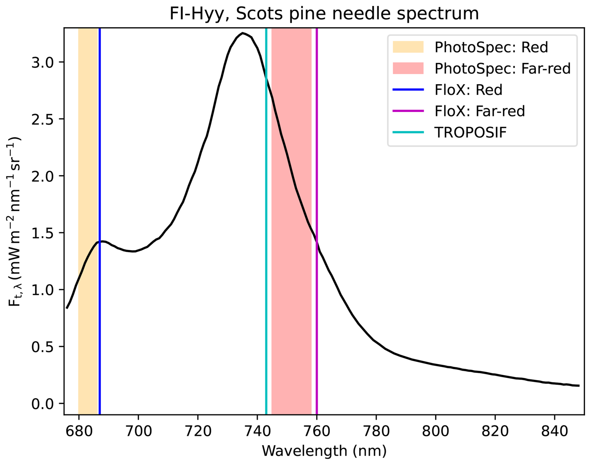
Figure 1 SIF emission spectrum for Scots pine located in the southern boreal zone (from Magney and Frankenberg, 2019) with wavelength regions of the observations. The lines indicate the bands for which the SIF signal was retrieved for the FloX observations and TROPOMI (TROPOSIF) and the shaded regions indicate the wavelength regions for which the SIF with the PhotoSpec was retrieved.

When moving from the leaf level to the canopy level, the interpretation of the measured signal becomes more challenging. Scattering and re-absorption and structural effects influence the SIF signal observed at the top of the canopy (Joiner et al., 2020; Malenovský et al., 2021; Paul-Limoges et al., 2018; van Der Tol et al., 2019) and also soil can contribute to the signal (Yang et al., 2025b). By using radiative transfer and biological modelling, mechanistic drivers of the SIF signal can be disentangled, improving our interpretation of SIF (Damm et al., 2015).

The use of SIF in vegetation modeling has become widespread. The first leaf-level description for ChlF was in FluorModLeaf (Miller et al., 2005). A wide-spread leaf level model that was further developed from FluorModLeaf was the Soil Canopy Observation of Photosynthesis and Energy fluxes (SCOPE) model (van der Tol et al., 2009). SCOPE is a site level model which combines the Farquhar photosynthesis model with a detailed radiative transfer scheme based on SAIL (van der Tol et al., 2009; Verhoef, 1984). Further developments have been done for the leaf level model used in SCOPE (van der Tol et al., 2014; Vilfan et al., 2016, 2018).

Recent model developments also allow the use of SIF to estimate GPP (Gu et al., 2019). These methods utilize the link between measured SIF and light reactions of photosynthesis and how these observations provide a link for actual electron transport from photosystem II to photosystem I. The model by Johnson and Berry (2021) has a tight coupling between photosynthesis and ChlF and allows estimating SIF from GPP and vice versa.

Terrestrial biosphere models (TBMs) are large-scale models used to study the biogeochemical cycles and land–atmosphere interactions. They can be run at a large scale (regional and global), but site-scale simulations are still possible. The modelling community has implemented SIF models in TBMs with varying degrees of complexity (e.g., Bacour et al., 2019; Koffi et al., 2015; Qiu et al., 2019; Thum et al., 2017). Some of these and other modelling studies have used also data assimilation (e.g., Bacour et al., 2019; Koffi et al., 2015; Wang et al., 2021).

These different approaches balance simplifying the complex physical phenomenon of radiative transfer in plant canopies against the length of the simulation time. However, full 1D radiative transfer based on the SCOPE model is too computationally demanding for many large scale applications (Sun et al., 2023a) and some modelling teams have needed to use parameterizations instead of the full model (Miyauchi et al., 2025). The computational burden becomes even more relevant in different data assimilation approaches (Norton et al., 2019). An empirical approach used in some studies would be worth investigating (Liu et al., 2020; Zeng et al., 2019). One way to simplify the calculation of SIF signal’s radiative transfer would be to use a two-stream radiative transfer model (Sun et al., 2023a). A recent two-stream radiative transfer model (Quaife, 2025) describes radiative transfer of emission originating from the canopy and therefore enables calculation of SIF signal’s radiative transfer. The TBM studies mentioned used spaceborne data from Greenhouse gases Observing SATellite (GOSAT) (Kuze et al., 2009),Orbiting Carbon Observatory (OCO)-2 (Frankenberg et al., 2014) and GOME-2 (Global Ozone Monitoring Experiment-2) (Munro et al., 2016).

The northern latitudes are experiencing stronger climatic change than the rest of the globe (Rantanen et al., 2022). Boreal forests located in these regions are an important part of the global carbon cycle (Pan et al., 2024). They are characterized by strong seasonality in environmental conditions, with harsh winter conditions and shoulder seasons when air and soil temperature and light availability drive the spring recovery and autumn drawdown of vegetation (Tanja et al., 2003; Thum et al., 2009; Vesala et al., 2010). The photosynthetic activity of evergreen forests in these ecosystems cannot be easily tracked by reflectance-based remote sensing alone, as the greenness is partially decoupled from the rate of photosynthesis (Walther et al., 2016). SIF observations have proven to be more reliable proxies for tracking photosynthesis in these ecosystems (Pierrat et al., 2024).

Challenging conditions have led evergreen trees to develop different coping mechanisms. Sustained NPQ is one of them and it increases in winter, at the same time as the capacity of photosystem II decreases (Porcar-Castell et al., 2008; Porcar-Castell, 2011; Adams et al., 2014). NPQ is a pH-independent mechanism associated with the retention of the xanthophyll cycle pigments zeaxanthin and antheraxanthin and allows the needles to dissipate the incoming radiation as heat (Demmig-Adams et al., 2014). Sustained NPQ can only be estimated from the active ChlF observations, i.e. when a set of saturating light pulses are delivered to a leaf under dark- and light-adapted conditions. Therefore, it cannot be directly obtained from passive SIF observations, although progress is being made towards optical sensing of NPQ (Van Wittenberghe et al., 2024). Including description of sustained NPQ in large scale TBMs was started by Raczka et al. (2019), who used the state of acclimation, represented by a delayed temperature sum developed by Mäkelä et al. (2004), in the parameterization.

The goal of this work was to improve the ChlF modelling so that a TBM can fully exploit the information provided by the ChlF related observations at different scales to improve our understanding of ecosystem processes related to biogeochemical cycles. Our objectives were (1) to test different radiative transfer approaches for SIF and (2) to assess the role of sustained NPQ in modelling. The research questions of our study are therefore:

• Which radiative transfer model calculation methods were sufficiently robust for reliable SIF model predictions?

• How could we account for the influence of sustained non-photochemical quenching in the modeled SIF signal across different sites?

• What was the benefit of in-situ observations versus satellite observations of SIF in model development?

To answer these questions, we run simulations of TBM QUINCY (“QUantifying Interactions between terrestrial Nutrient CYcles and the climate system”) (Thum et al., 2019) with different radiative transfer approaches and compared them with tower observations of SIF at three coniferous evergreen sites that experience a strong seasonal cycle with harsh winters. In addition, we tested how spaceborn TROPOspheric Monitoring Instrument (TROPOMI) instrument (on board the Sentinel-5 Precursor (S5P) satellite) (Guanter et al., 2021) data capture the seasonal cycle at two of these sites and how its magnitude differs from the simulation results. The novel aspects of this study include using different radiative transfer schemes with one model, analyzing both red and far-red region observations from the tower observations of SIF, having sites in two different continents and having approaches that either include the SIF signal attenuation inside the leaf or not. Including both red and far-red regions in the analysis will help to evaluate potential challenges that the simulations will have in the red region, a fact that will become more relevant with new satellite missions covering whole SIF spectrum, such as The Fluorescence Explorer (FLEX) (Moreno, 2022).

2 Materials and methods

2.1 Site descriptions

The three study sites were Niwot Ridge (US-NR1), USA (Bowling et al., 2018; Burns et al., 2015; Magney et al., 2019a), Saskatchewan (CA-Obs), Canada (Pierrat et al., 2021, 2022a) and Sodankylä (FI-Sod), Finland (Thum et al., 2007; Knorr et al., 2025). All of these sites are evergreen coniferous forests. The Canadian and Finnish sites are in the boreal zone, and Niwot Ridge is a subalpine forest. Further details about the sites are given in Table 1. All sites have eddy covariance flux observations as well as a tower-mounted in-situ SIF instrument. The Sodankylä site is part of the ICOS network (https://www.icos-cp.eu/, last access: 1 September 2025) and the North American sites are part of AmeriFlux (https://ameriflux.lbl.gov/, last access: 1 September 2025).

Although all of these sites exhibit a strong seasonal cycle in vegetation activity, this varies due to differences in latitude and elevation. The forest in CA-Obs exhibit a strong seasonal cycle, characterized by low levels of photosynthetic activity between October and March. Although US-NR1 is located at a lower latitude than the other study sites, high elevation conditions result in a pronounced seasonal cycle, including winter below freezing temperatures. Photosynthesis in the forest at US-NR1 is active from May to September, with the shoulder season to winter occurring in October and November, and the spring recovery occurring in April and May. FI-Sod is located 100 km north of the Arctic Circle. Therefore, the winter radiation drops to zero, and air temperatures are low. Spring recovery occurs in April and May. The photosynthetically active period is from June to August and photosynthesis ceases in September and October.

Table 1 The site characteristics of the three forests. LAI is one-sided and average value over summertime. Air temperature is annual average.

2.2 SIF and CO₂ flux observations at the sites

At the North American sites, SIF was observed with PhotoSpec (Grossmann et al., 2018) in two different spectral regions. The red region of PhotoSpec is between 680 and 686 nm, and the far-red region is between 745 and 758 nm. These observations were made with a 2D scanning telescope. The retrieval method was based on the Fraunhofer line method (Grossmann et al., 2018). The field of view (FOV) was 0.7°. At US-NR1 a typical measurement involved scanning from nadir to the horizon in steps of 0.7° at two different azimuth directions (Magney et al., 2019a). At CA-Obs three vertical scans at three different directions (35° W, 0° N, 35° E) were done in sequence (Pierrat et al., 2021). The PhotoSpec retrievals were filtered using a Normalized Difference Vegetation Index (NDVI) based threshold to ensure that only vegetation observations were used. In this study we averaged over all the three scans. Further details of these observations can be found in Magney et al. (2019a) (US-NR1) and Pierrat et al. (2021) (CA-Obs). At US-NR1, observations were available from June 2017 to June 2018. At CA-Obs we used observations from the whole of 2019 and 2020.

In Sodankylä, the observations were made using a FloX box (JB Hyperspectral Devices, Düsseldorf, Germany) (https://www.jb-hyperspectral.com/products/flox/, last access: 1 September 2025). These observations were used to retrieve the SIF in the O₂B band at 687 nm in the red region and theO₂A band at 760 nm in the far-red region. The retrieval method used to process the data was the improved Fraunhofer line method (Alonso et al., 2008; Cendrero-Mateo et al., 2019). In our study, we used observations close to nadir from June 2021 until the end of the year. The FOV is 25°. The different wavelengths of the retrieved SIF signals by the instruments are shown in Fig. 1, along with the SIF spectrum from observations of Scots pine needles in Hyytiälä, southern Finland (Magney and Frankenberg, 2019; Magney et al., 2019b).

Net ecosystem exchange of CO₂ was measured by the eddy covariance method. At CA-Obs the measurement height was 25 m, and the anemometer was CSAT3 (Campbell Scientific Inc., Logan, UT, USA) and the gas analyzer LiCor LI-7200 (LiCor Inc., Lincoln, NE, USA) (Pierrat et al., 2021). In spring 2019 the eddy covariance observations at CA-Obs were out of commission and until mid-2019 the GPP data was based on gap–filling. At US-NR1 measurements were made at 21.5 m height with the CSAT3 and an LiCor LI-6262 gas analyzer (Magney et al., 2019a). At FI-Sod, measurements were made at 25 m with a Gill HS-50 sonic anemometer (Gill Instruments, Lymington, UK) and a LiCor LI-7200 gas analyzer (Knorr et al., 2025). Flux partitioning and gap–filling at CA-Obs was done as described in Barr et al. (2004) and at US-NR1 using the Reichstein et al. (2005) method with the R package REddyProc (Wutzler et al., 2018). Gap–filling and partitioning of the measured net ecosystem exchange flux to gross primary production (GPP) and total ecosystem respiration was done at FI-Sod following Aurela et al. (2015). In Sodankylä, the fraction of absorbed photosynthetically active radiation (fAPAR) was measured using PQS1 instruments (Kipp & Zonen; Netherlands) (Knorr et al., 2025). Four of these sensors were installed below the canopy. These observations, together with aboveground canopy observations, were used to calculate fAPAR.

2.3 Remote sensing observations of SIF by TROPOMI

The TROPOMI is aboard the Copernicus Sentinel-5P mission and has been providing data since 2018 (Köhler et al., 2018). TROPOMI provides global, continuous spatial sampling with a daily revisit time because it has a nearly sun-synchronous orbit with a 16 d repeat cycle and a 2600 km swath (Köhler et al., 2018). The pixel size at nadir was 3.5×7.5 km² at the beginning of the mission, decreasing to 3.5×5.5 km² after August 2019 (Guanter et al., 2021). We used the TROPOSIF product derived from the 743–758 nm window, at 740 nm (Guanter et al., 2021). The retrieval methodology was based on the Fraunhofer line in-filling principle (Plascyk and Gabriel, 1975) and a data-driven method was used (Guanter et al., 2015).

In this study we used a sampling area of 0.5° × 0.5° around the two study sites, CA-Obs and FI-Sod. This corresponds to an area of approximately 56 km × 33 km at CA-Obs and 56 km × 22 km at FI-Sod. According to the 2019 MODIS MCD12C1 data set (Friedl and Sulla-Menashe, 2022), the land cover for CA-Obs in this region was 65 % woody savannah and 26 % evergreen needleleaf forest, with minor contributions from mixed forests and croplands. For FI-Sod, the land cover was 83 % woody savannah and 17 % savannah. We also tested a smaller sampling area extending 0.25° around the site. In this smaller region, the land cover around CA-Obs was 45 % evergreen forest and 53 % woody savannah, with a small contribution from mixed forests. For the FI-Sod site the smaller region comprised of 92 % woody savannah and 8 % of savannah. We did not use TROPOMI data for US-NR1 because TROPOMI observations only covered part of the in situ observational period. TROPOMI's Level 2 cloud fraction product was applied for a strict cloud filtering, removing all SIF data for which the cloud fraction exceeded 0.2, as recommended by Guanter et al. (2021). For our analysis, we used daily averages that we had calculated from instantaneous values.

2.4 Model description of QUINCY

The QUantifying Interactions between terrestrial Nutrient CYcles and the climate system (QUINCY) model is a terrestrial biosphere model that can be run on a single site or on larger scales, such as regional or global. QUINCY uses plant functional types (PFTs) to describe different ecosystems. In site level simulations, each site is represented by a single PFT. Canopy can have up to ten layers. A brief description of the model is provided here; further details can be found in Thum et al. (2019).

The complete version of QUINCY features fully coupled carbon, energy, nitrogen and phosphorus cycles. The model has a modular structure that allows only some parts of the model to be run. We used the canopy module, which calculates the model's fast biophysical processes, including stomatal conductance, photosynthesis and radiative transfer within the canopy. Influence of the soil is also considered, so that water uptake is constrained by soil moisture given a prescribed, PFT-specific root profile. The leaf area index (LAI) and leaf nitrogen content are prescribed with a constant value in the canopy module (otherwise these would be calculated prognostically inside the model). Leaf stoichiometry, i.e. the nitrogen to carbon ratio, is also fixed in the canopy module. The calculation of leaf chlorophyll from leaf nitrogen is described in Sect. S1.1 in the Supplement.

Photosynthesis is calculated according to Kull and Kruijt (1998). This approach is based on the biochemical model of Farquhar et al. (1980), but instead of the regular implementation of having the minimum of the two branches limiting photosynthesis (light-limited rate of photosynthesis and carboxylation capacity limited rate), the amount of light-saturated region in the leaf is taken into account. In the non-light-saturated part, photosynthesis is calculated using the light-limited rate of photosynthesis based on the maximum electron transport rate parameter J_max,25 (the parameter has been scaled to 25 °C). For the light-saturated part, photosynthesis is calculated as the minimum of electron transport rate-limited photosynthesis and the carboxylation capacity limited photosynthesis (determined by the maximum carboxylation capacity parameter V_c(max),25). Photosynthesis is calculated separately for sunlit and shaded leaves in each canopy layer and coupled to the stomatal conductance (Medlyn et al., 2011), described in Sect. S1.2. Evergreen trees in cold environments adapt their photosynthesis during the shoulder seasons as described in Sect. S1.3.

2.4.1 Radiative transfer in QUINCY

The depth (in terms of LAI) of the canopy layers increases exponentially towards the lower canopy layers. The nitrogen gradient decreases with canopy depth according to observations (Niinemets et al., 1998), but is not connected to the leaf optical properties in the current model formulation. The fraction of sunlit and shaded leaves is calculated using a radiative transfer scheme based on the two-stream approach of Spitters (1986) and extended to include canopy albedo, clumping, and attenuation of the shortwave backscatter from the ground. Radiative transfer is calculated separately for the visible (300–700 nm) and near-infrared (700–3000 nm) bands. Leaf reflectance is calculated based on the PFT-specific single leaf scattering albedo (SSA). Leaf transmissivity is assumed to be equal to reflectivity, and absorptance is defined as one minus SSA. The clumping index (Ω), which describes non-random distribution of leaf elements, is defined according to Campbell and Norman (1998):

$$\begin{array}{}\text{(1)}& \mathrm{\Omega }={\mathrm{\Omega }}_{\mathrm{0}}/({\mathrm{\Omega }}_{\mathrm{0}}+(\mathrm{1}-{\mathrm{\Omega }}_{\mathrm{0}})\times e^{-k_{\mathrm{csf}}\times \mathrm{acos}({\mathit{\gamma }}^{*}{)}^{{\mathit{\varphi }}_{\mathrm{crown}}}}),\end{array}$$

where Ω₀ and ϕ_crown are the PFT-specific clumping factor at nadir (0.5 for conifers) and the crown shape factor (2.19 for conifers), respectively, and k_csf is a correction factor with a value of 2.2. A seasonal cycle of Ω at FI-Sod is shown in Fig. S1 in the Supplement. As all equations for leaf reflection and absorption coefficients are only valid for high solar elevation, the true zenith angle (γ) is constrained to values smaller than 80° (γ^*), i.e. it will receive a value of 80° in the event of a higher zenith angle. Otherwise, the leaves are assumed to be distributed spherically. The soil albedo is set to a literature value for the visible and near infrared regions (Bonan, 2008).

2.5 Models for the radiative transfer of the SIF signal

The leaf chlorophyll fluorescence yield was calculated using the model developed by van der Tol et al. (2014). The equations can be found in Sect. S1.4. We did not change any of the model's default parameter values and these parameters were kept constant across all sites. The only change to the standard implementation of the model was caused by the different Farquhar et al. model formulation adapted for use with QUINCY, which did not require any additional parameters.

The escape fraction describes how much of the emitted SIF signal reaches the top of the canopy. The total canopy SIF can be expressed using the escape fraction f_esc as (Sun et al., 2017):

$$\begin{array}{}\text{(2)}& \mathrm{SIF}=\mathrm{PAR}\cdot \mathrm{fAPAR}\cdot {\mathrm{\Phi }}_{F_t}\cdot f_{\mathrm{esc}}\end{array}$$

where SIF is the observed SIF, PAR is the photosynthetically active radiation, fAPAR is the fraction of absorbed PAR and ${\mathrm{\Phi }}_{F_t}$ is the chlorophyll fluorescence yield. This section introduces the three different approaches to calculating radiative transfer of SIF in the canopy that were used in this study. The first approach uses the mSCOPE model, which has been incorporated into the QUINCY model. This hyperspectral approach considers the attenuation of the SIF signal within the leaf. Rather than being implemented in QUINCY, the L2SM model uses QUINCY's output. In our case, it utilizes two spectral regions (visible below 700 nm regions and near infrared for above 700 nm). This approach considers the attenuation of the SIF signal within the leaf. The final approach is based on an empirical relationship and estimates the escape fraction using the fraction of absorbed PAR and leaf reflectance obtained from QUINCY, which considers the visible and near infrared regions in the same way as L2SM. All approaches treat SIF emission as a diffuse flux.

2.5.1 mSCOPE

The mSCOPE model (Yang et al., 2017) is a further development of the widely used SCOPE model (van der Tol et al., 2009) that has been eventually implemented in SCOPE 2.0 (Yang et al., 2021). In mSCOPE, the canopy structure is permitted to have a heterogeneous vertical canopy structure, whereas in SCOPE it is assumed to be homogeneous. The QUINCY model has a vertically varying canopy structure, as explained in Sect. 2.4. Therefore, the use of mSCOPE was more suitable than SCOPE for coupling with QUINCY.

In mSCOPE, the Fluspect model (Vilfan et al., 2016) calculates leaf reflectance, transmittance and ChlF. The radiative transfer of mSCOPE is described by two SAIL-based models (Verhoef, 1984): one, which calculates the radiative transfer of incident radiation, and another one, which calculates the radiative transfer of emitted ChlF. Homogeneity is assumed in the horizontal direction, but heterogeneity of leaf properties is allowed in the vertical direction. The probability of sunlight on leaves is described by a Poisson model. Shaded leaves are illuminated only by diffuse radiation, so their absorbed radiation does not depend on geometry. For the sunlit leaves, the absorbed radiation is calculated for discrete leaf orientations, including 13 leaf inclinations and 36 leaf azimuth angles relative to the solar azimuth. Soil optical properties are represented by a linear combination of a dry and a saturated soil reflectance factors, weighted as a function of the ratio of soil moisture content to field capacity. The mSCOPE model calculates the top of the canopy (TOC) value for ChlF emission.

The mSCOPE model has been implemented in QUINCY (see the conceptual figure in Fig. S2). This implementation replaces the original QUINCY radiative transfer model (Spitters, 1986). The vertical profile of leaf chlorophyll, which was calculated in QUINCY (S1.1), was used to calculate the radiative properties of each layer. To calculate this, mSCOPE uses the PROSPECT model (Jacquemoud and Baret, 1990). mSCOPE runs over 60 canopy layers, that were grouped to mimic the usual 10 layers in QUINCY as a function of the QUINCY layer LAI. The mSCOPE outputs were then integrated for each layer group to represent each of the 10 QUINCY layers. For stability reasons, we also limited the calculation of the radiative transfer code to solar zenith angles below 80°. To test the implementation, we performed a sensitivity analysis by running simulations with different parameter values in both mSCOPE and QUINCY-mSCOPE. The results were consistent (not shown). We are therefore confident that there are no major technical errors in the implementation. Using QUINCY with mSCOPE instead of QUINCY with the original radiative transfer model caused minor differences in the simulated GPP, but the overall results were similar (for CA-Obs the Pearson correlation coefficient (r²) was 0.99 for half-hourly values throughout the time period and the root mean squared error (RMSE) was 0.77 $\mathrm{\mu }\mathrm{mol}{\mathrm{m}}^{-\mathrm{2}}{\mathrm{s}}^{-\mathrm{1}}$). The viewing angle was set to nadir in these simulations.

2.5.2 Layered two-stream model (L2SM)

The Layered canopy two-Stream Model (L2SM) (Knorr et al., 2025; Quaife, 2025) is a two-stream radiative transfer model based on the solutions provided by Meador and Weaver (1980). It allows the calculation of diffuse emissions originating from plant leaves. A conceptual figure showing how it is used in combination with QUINCY is shown in Fig. S3, and the equations of the model are in Sect. S1.5. The formulation of L2SM is a two-stream model, similar to the original radiative transfer model of QUINCY. Consequently, it calculates the radiative transfer in the visible and near infrared regions separately. Soil reflectance was assumed to be isotropic and leaf angle distribution was assumed spherical. We used L2SM with the leaf reflectance (which also equals transmissivity in QUINCY), the leaf area index for each layer, and the SIF emission per layer (as calculated by Eq. S15) as well as information on soil reflectance. In this implementation a novelty was that internal attenuation of the SIF signal was taken into account. While QUINCY is based on Spitters (1986), the L2SM approach is based on Meador and Weaver (1980). Therefore, the radiative transfer of incoming radiation used to calculate photosynthesis differs slightly from the way SIF is transferred within the canopy. A detailed derivation and description of the L2SM can be found in Quaife (2025).

2.5.3 Liu and Zeng approaches (LZ)

In addition to modelling the transfer of the SIF signal, we have also tested some simpler formulations to estimate the SIF leaving the canopy. A more empirical approach was based on the work of Liu et al. (2020) (for the visible region) and Zeng et al. (2019) (for the near-infrared/far-red region). We used the formulation presented by Hao et al. (2021) for the escape fraction (a conceptual figure is shown in Fig. S4 and see Eq. 2). An empirically based formulation for the escape fraction f_esc is:

$$\begin{array}{}\text{(3)}& f_{\mathrm{esc}}^{\mathrm{reg}}={\displaystyle \frac{{\mathit{\rho }}_{\mathrm{can}}^{\mathrm{reg}}}{\mathrm{fAPAR}\cdot {\mathit{\sigma }}^{\mathrm{reg}}}}\end{array}$$

where reg is either visible (vis) or near-infrared (nir) region, ρ_can is the reflectance of green vegetation and σ is the single leaf scattering albedo (SSA). Therefore, this escape fraction is calculated separately for the visible and the near-infrared regions. The soil was assumed to be black, i.e. non-reflectant. To estimate the escape fraction from QUINCY in this way, we used the modelled vegetation reflectance for the entire canopy, fAPAR and the constants for single-leaf scattering albedo. After calculating the escape fraction, the upscaled SIF emission (calculated as the sum of canopy layer SIF emissions from Eq. (S15) which were multiplied by the canopy LAI) was multiplied by it to obtain the estimated SIF signal.

2.6 Converting the units of SIF from modelled to observed

The output of the radiative transfer approaches in Sect. 2.5.2–2.5.3 is in flux units, i.e. $\mathrm{\mu }\mathrm{mol}{\mathrm{m}}^{-\mathrm{2}}{\mathrm{s}}^{-\mathrm{1}}$. To be able to compare the model output with the observations, which are typically in units of ${\mathrm{Wm}}^{-\mathrm{2}}{\mathrm{s}}^{-\mathrm{1}}{\mathrm{nm}}^{-\mathrm{1}}{\mathrm{sr}}^{-\mathrm{1}}$, we need to convert the units of the model output. This procedure was similar as described in Knorr et al. (2025) and also in Sect. S1.7. The QUINCY run with mSCOPE provides ChlF directly within the observed units, and is therefore independent of this approach.

2.7 Sustained non-photochemical quenching (NPQ_s)

Sustained non-photochemical quenching (NPQ_s) is a process that is relevant to evergreen plants. This is another NPQ mechanism in addition to the reversible NPQ that we introduced in the Sect. S1.4 (Eq. S14). In previous work with the Community Land Model (CLM) model (Raczka et al., 2019), a parameterization for sustained NPQ based on the state of acclimation was developed. We have previously used the concept of the state of acclimation in the QUINCY photosynthesis model (Eq. S5). Following the earlier work and similarly to the state of acclimation, we obtained for $K_{N_{\mathrm{s}}}$:

$$\begin{array}{}\text{(4)}& K_{N_{\mathrm{s}}}={\displaystyle \frac{K_{N_{\mathrm{s},\max }}}{\mathrm{1}+e^{b_{{\mathrm{NPQ}}_{\mathrm{s}}}(S-T_{{\mathrm{NPQ}}_{\mathrm{s}}})}}}\end{array}$$

where $K_{N_{\mathrm{s},\max }}$, ${\mathrm{b}}_{{\mathrm{NPQ}}_{\mathrm{s}}}$ (°C⁻¹) and $T_{{\mathrm{NPQ}}_{\mathrm{s}}}$ (°C) are parameters, set to 8.0, 0.5 °C⁻¹ and 5.0 °C, respectively. The difference between this equation and Eq. (S5) is that it has large values in winter, while Eq. (S5) has large values during the summer. S is obtained from Eq. (S4). To estimate the parameters in the Eq. (4) we used SIF observations from US-NR1 and adjusted the parameter values to achieve the best possible match with our model over the entire observational period. A seasonal cycle of $K_{N_{\mathrm{s}}}$ and S at Sodankylä in 2021 are shown in Fig. S5.

When both reversible and sustained NPQ were taken into account, K_N was then a sum of them, as

$$\begin{array}{}\text{(5)}& K_N=K_{N_{\mathrm{rev}}}+K_{N_{\mathrm{s}}}.\end{array}$$

2.8 Site scale flux simulation protocol

All the sites in the study were classified as a boreal coniferous evergreen forests PFT in QUINCY. For this study we took advantage of the modular structure of QUINCY and only used the canopy model in our simulations. The LAI and leaf nitrogen content were set to ensure that the average summertime GPP level corresponded with the observed values. The meteorological data (air temperature, precipitation, atmospheric pressure, vapor pressure deficit, wind speed, short and longwave radiation) required to run the model were obtained from the site measurements. In addition, we used atmospheric CO₂ concentration and N deposition, although the N cycle was not active in the canopy model simulations. The canopy model does not require any spinup, and the simulations were performed for the years of the observations. The leaf single scattering albedo used to calculate reflectance for conifers was 0.15 in the visible wavelength region and 0.73 in the near infrared (Otto et al., 2014). The soil albedo for all the sites was estimated to be 0.15 in the visible and 0.30 in the near infrared. The LAI values were set to lower than the observed values to better match the observed magnitude of GPP. The LAI was set to 2.5 m² m⁻² in CA-Obs, 3.6 m² m⁻² in US-NR1 and 1.2 m² m⁻² in FI-Sod. When presenting the results in Sect. 3.1, we had used the sustained NPQ presentation for the CA-Obs and US-NR1 sites, but not for the FI-Sod site.

2.9 Evaluation methodology

The metrics to assess the model performance were coefficient of correlation (r²) (Wright, 1921), bias and root mean square error (RMSE) (Hastie et al., 2009) as well as its systematic and random components (Willmott, 1981). These formulas have been shown in Sect. S1.6.

For many of the figures we used averaging window of 15 d to smooth out the daily values, so that the seasonal cycle would be easier to distinguish. We showed for the subdaily time scale separately metrics for the model performance on morning (06:00 to 09:30 a.m., local winter time), midday (10:00 a.m. to 01:30 p.m.) and afternoon (02:00 to 05:30 p.m.). All of these times were local winter time.

As the mSCOPE was run inside QUINCY, while the two other approaches were run outside, the wall time calculation differed. For the mSCOPE version, the wall time was calculated as the time it took for QUINCY to simulate one year at FI-Sod. For the L2SM and the LZ approaches, QUINCY was first run for one year at FI-Sod. Then the calculation performed outside QUINCY in Python was added to this wall time value.

3 Results

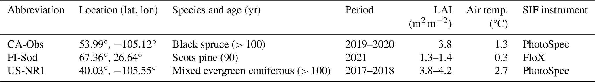
The diurnal monthly cycles and the seasonal cycles of the observed and simulated SIF signals for the years 2019 and 2020 at CA-Obs are shown in Fig. 2. This was the final result we obtained after testing for different radiative transfer schemes and adding the description for sustained NPQ. The following sections describe how we arrived at these results. In the main text, we focus on the results from the CA-Obs site, for which we had the most data. In the Supplement, we present the results for the other two sites.

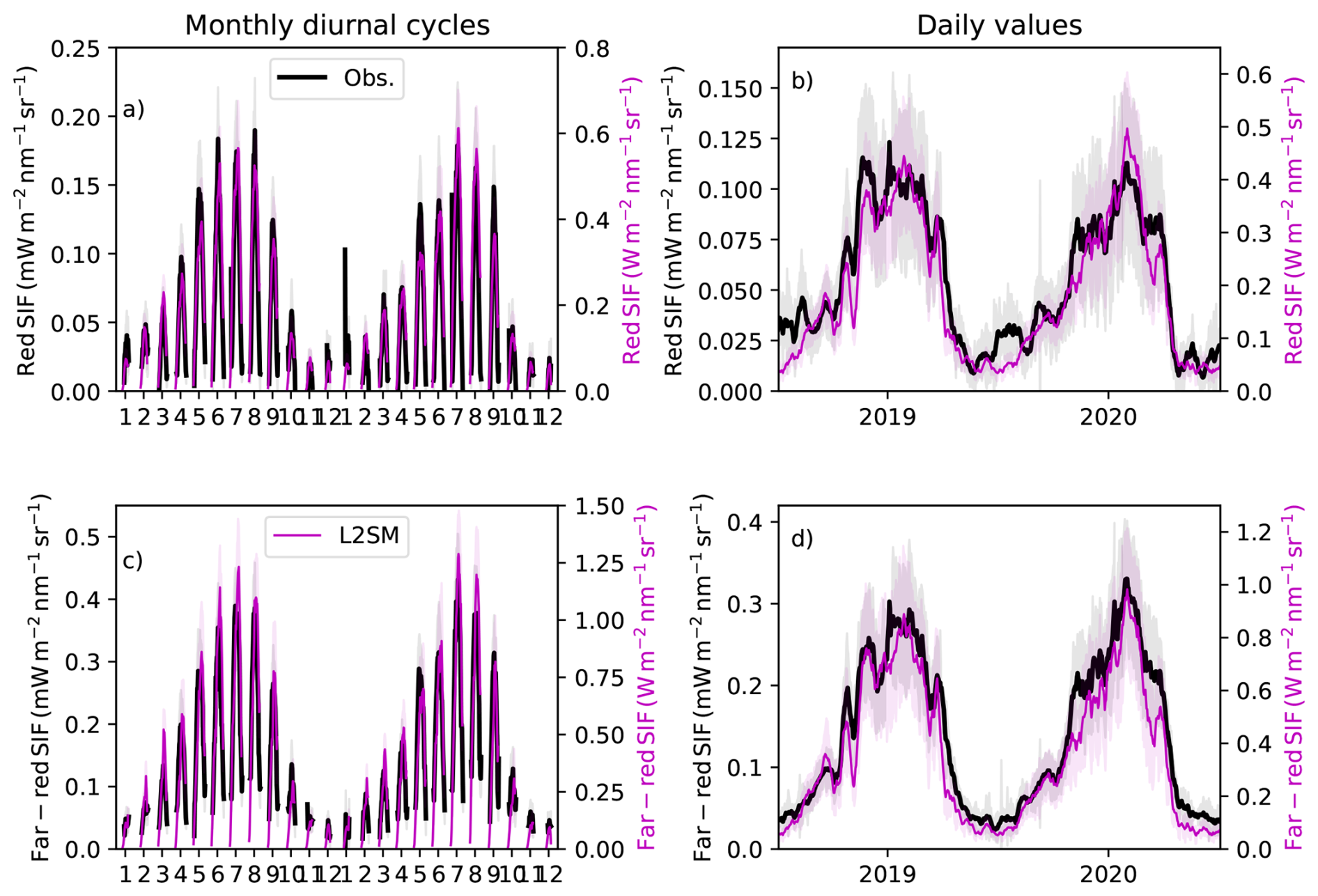
Figure 2 Monthly diurnal cycles for (a) red region SIF and (c) far-red SIF and daily values for (b) red region SIF and (d) far-red SIF at CA-Obs. The black line is the observation for all plots, magenta for the L2SM. All the lines for daily values have been smoothed with a 15 d long window. The shaded regions denote standard deviation.

3.1 Performance of the radiative transfer models

3.1.1 CA-Obs

The monthly diurnal cycles and midday values (10:00 a.m. to 01:30 p.m.) for GPP, red region SIF and far-red SIF at CA-Obs (Fig. 3) showed large overestimation with all the different SIF transfer schemes. The midday values are shown here to give a better insight into how the magnitude of the variables changes, thus removing the strong influence of the change in day length on the results. QUINCY was able to capture the seasonal behaviour at the site. The large overestimation of the SIF simulation results will also be discussed later in this paper.

Figure 3 Monthly diurnal cycles for (a) GPP, (c) red region SIF and(e) far-red SIF and midday values, calculated from winter time between 10:00 a.m. and 01:30 p.m., for (b) GPP, (d) red region SIF and (f) far-red SIF in CA-Obs. The black line is the observation in all plots, the pink line in the GPP plots is the QUINCY simulation. For the SIF plots the red line is the mSCOPE result, cyan the L2SM and blue the LZ approach. All the lines for midday values have been smoothed with a 15 d long window.

The model performance of GPP in CA-Obs was generally good (Table 2). The simulation of GPP was best at midday, and slightly less in morning hours. Since there was a long gap in observed GPP in 2019 and we instead used gap–filled GPP, we also checked the r² of daily GPP values for the two years separately. For 2019 the r² was 0.89 and for 2020 0.86, possibly reflecting the fact that simulations did not capture the turbulent nature of eddy covariance observations, but were potentially closer to gap–filled values that estimate the average behaviour of the ecosystem.

Table 2 The r² and RMSE values of simulated versus observed SIF values in the red and far-red regions in 2019–2020, according to different radiative transfer approaches at CA-Obs. The metrics are also shown for the GPP derived from the standard QUINCY configuration. The morning values are from 06:00 a.m. to 09:30 a.m., the midday values from 10:00 a.m. to 01:30 p.m., and the afternoon values from 02:00 to 05:30 p.m.

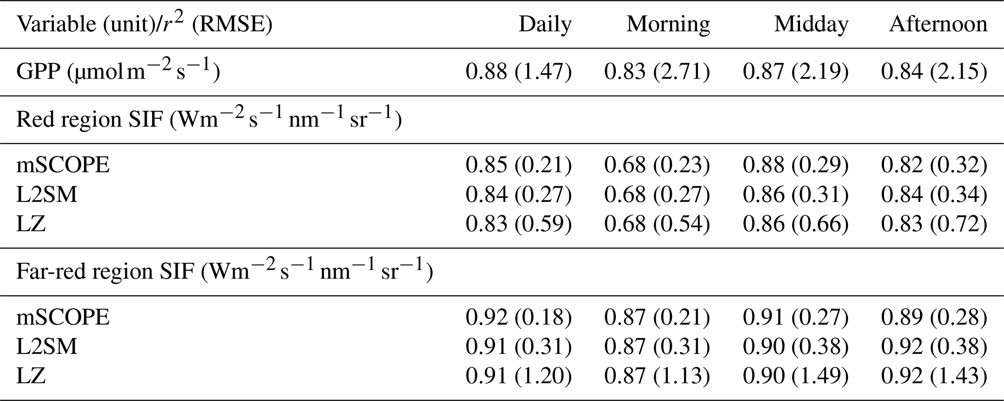
The daily r² values for SIF were close to those of GPP (Table 2). Overall, modelling of SIF was more successful in the far-red region than in the red region. The r² values in both wavelength regions were better in the midday and afternoon than in the morning. When investigating whether the different months showed clearly different patterns in model behaviour (Fig. 4), it was seen that the highest simulated midday values in summer were higher than the linear fit between observations and simulations would imply, suggesting that the model had a tendency to overestimate these values relative to other time periods.

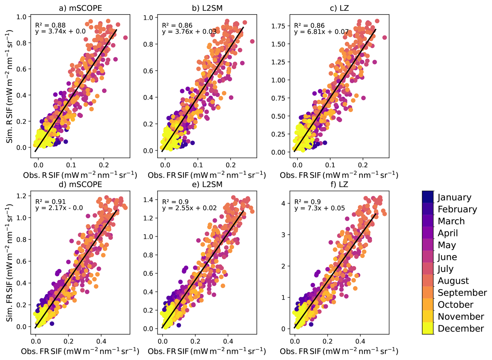
Figure 4 Observed vs. modelled SIF midday values in the red (denoted with R in the figure) region (a: mSCOPE, b: L2SM, c: LZ) and far-red (denoted with FR in the figure) region (d: mSCOPE, e: L2SM: f: LZ) at CA-Obs. Values from different months are color-coded. The black line shows a fit with the corresponding parameters shown in each panel.

The performance of the different modelling approaches was quite comparable when looking at the r² values (Table 2). The RMSE values showed greater variation. Overall, the r² values were quite similar between the approaches, showing that the different approaches did not have a pronounced influence on the temporal patterns of the simulated SIF.

3.1.2 US-NR1 and FI-Sod

Running the same simulations at other sites enabled us to evaluate the model's performance further and to consider the possible influence of instrumentation on the diurnal dynamics. The model performance for simulating GPP and SIF was lower in US-NR1 than in CA-Obs (Table S2 in the Supplement, Fig. S6). For SIF this is clearly seen in the amount of scatter between simulated and observed values in Fig. S7. The model seemed to have difficulty in capturing the variation in midday values during the summer months. The seasonal cycle of SIF in US-NR1 was not as well reproduced as in CA-Obs (Fig. S6b vs. Fig. 5b), although the spring recovery of GPP seemed to be well simulated (Fig. S5b). Similar to CA-Obs, the r² values for SIF were generally higher in the far-red region than in the red region at US-NR1 (Table S2). The model performance was best at midday.

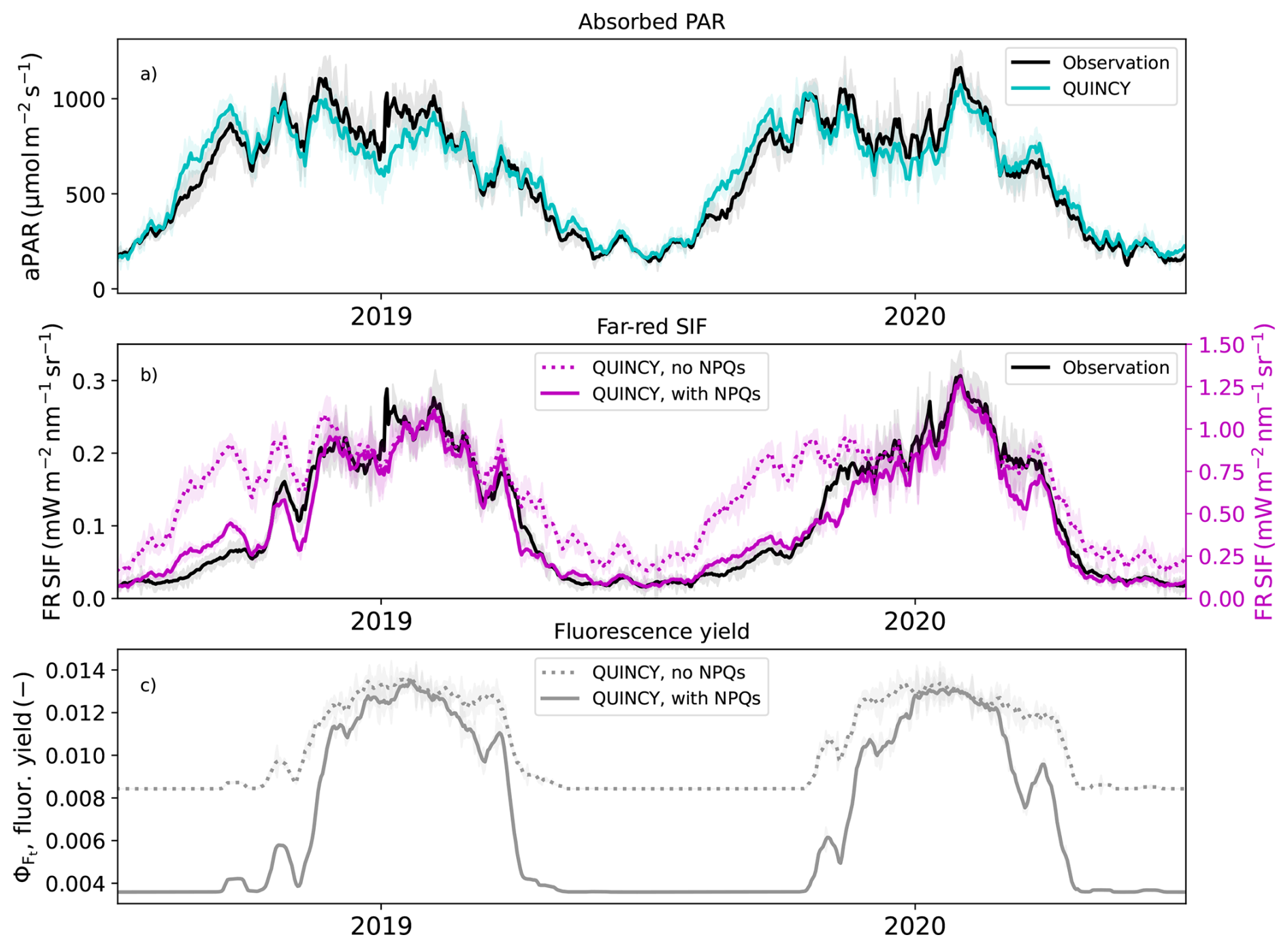
Figure 5 (a) The observed and simulated absorbed photosynthetically active radiation at CA-Obs, (b) far red (FR) region SIF values with and without sustained NPQ simulated with L2SM and (c) simulated chlorophyll fluorescence yields with and without sustained NPQ. Values are averages of midday values (10:00 a.m. to 01:30 p.m.), the standard deviation is shown as shaded areas. All the lines for midday values were smoothed with a 15 d long window.

QUINCY was more successful in simulating GPP at FI-Sod than at the other two sites (Fig. S8, Table S3). Modelling SIF was less successful than modelling of GPP in FI-Sod (Table S3, Fig. S9). In both spectral regions, the model performed best in the morning and midday, and worse in the afternoon. Differences between the radiative transfer approaches were not pronounced.

3.1.3 Performance comparison

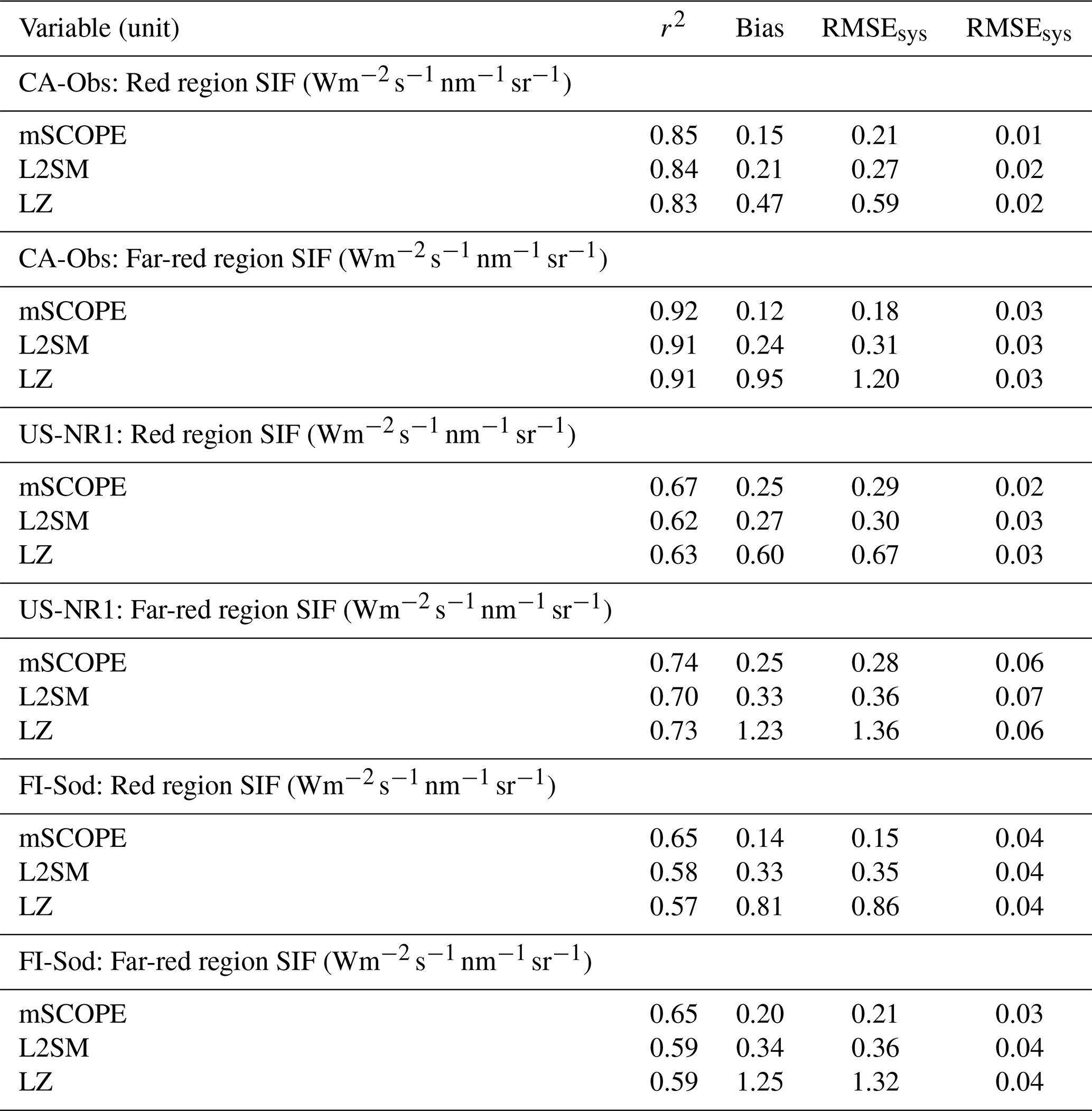
The magnitude of the observed SIF was similar in both the red and far-red regions at the two sites with the PhotoSpec observations (Table S4) for the July–August midday values. Compared to these values, the FI-Sod value observed with FloX was higher in the red region and lower in the far-red region, which was consistent with what we see in the spectral shape of the SIF emission (Fig. 1). In the far-red region this difference was more pronounced and was half of the value observed with PhotoSpec (Table S4). The overestimation of SIF by the different radiative transfer methods was most pronounced for the sites with PhotoSpec observations in the red region. In the far-red region, mSCOPE had the lowest overestimation, while the LZ approach had the highest. The same was true when looking at the metrics for all the sites combined (Table 3). The LZ approach had the highest bias and systematic RMSE across the sites. Otherwise, generally mSCOPE had the best performance metrics, but the other approaches were not much worse.

Table 3 The r², bias, RMSE_sys and RMSE_ran values of simulated versus observed SIF values in the red and far-red regions according to different radiative transfer approaches at the three sites. The metrics are also shown for the GPP derived from the standard QUINCY configuration. The values are calculated on daily values.

As the simulation time is important for large scale applications, we calculated the wall times for the simulations for one year at FI-Sod. LZ (with a wall time of 10 s) was 419 times faster than the mSCOPE approach (with a wall time of 4191 s), while L2SM (with a wall time of 20 s) was 210 times faster than the mSCOPE approach.

3.2 Importance and generality of sustained NPQ modelling

SIF modelled without sustained NPQ showed a strong relationship with the absorbed PAR (aPAR) at CA-Obs (Fig. 5a). A CA-Obs simulation was done to evaluate the performance of the parameterization carried out at US-NR1. QUINCY successfully simulated the aPAR at CA-Obs at midday (Fig. 5a, Table 4). The seasonal cycle was strong, with winter aPAR values around 200 $\mathrm{\mu }\mathrm{mol}\mathrm{photons}{\mathrm{m}}^{-\mathrm{2}}{\mathrm{s}}^{-\mathrm{1}}$. The increase towards summer aPAR values started earlier than the observed GPP increase, as low temperatures prevented the spring recovery of vegetation. The increase in aPAR towards summer values started in the first part of the year, much earlier than the increase in SIF values (Fig. 5). The simulated SIF, without the described NPQ_s, followed the behaviour of the aPAR. The simulated SIF with the NPQ_s was more similar to the observed seasonal behaviour (Fig. 5b, Table 4). While the magnitudes differed between the simulations and observations for SIF, the general timing was better for the simulation with NPQ_s. The NPQ_s had a strong influence on the chlorophyll fluorescence yield (Φ_F) in the model (Fig. 5c).

Table 4 The metrics (r², RMSE and bias) of the simulated absorbed PAR (aPAR) and far-red region (FR) SIF at the three sites for midday values with and without the formulation for NPQ_s. The units of RMSE and bias are ${\mathrm{Wm}}^{-\mathrm{2}}{\mathrm{s}}^{-\mathrm{1}}{\mathrm{nm}}^{-\mathrm{1}}{\mathrm{sr}}^{-\mathrm{1}}$ for far-red region SIF and $\mathrm{\mu }\mathrm{mol}{\mathrm{m}}^{-\mathrm{2}}{\mathrm{s}}^{-\mathrm{1}}$ for APAR.

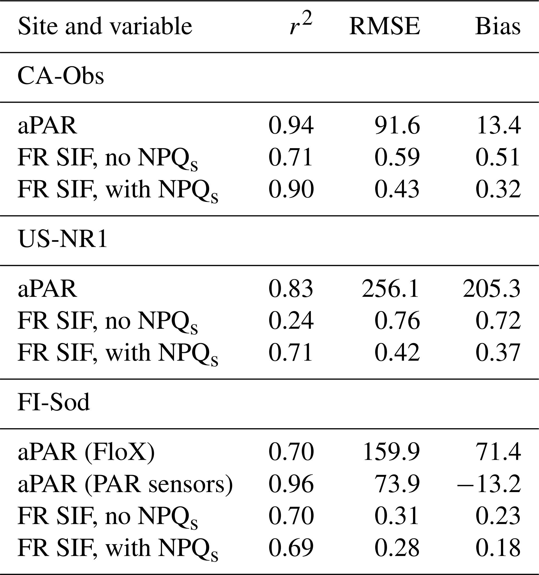
As US-NR1 is located further south than CA-Obs, the aPAR did not exhibit a pronounced seasonal cycle (Fig. S10a). The simulated SIF without NPQ_s followed the seasonal cycle of aPAR. To simulate the seasonal variation observed in SIF, it was necessary to include NPQ_s in the modelling. However, the formulation used for NPQ_s delayed the spring recovery in 2018 by too much. The formulated NPQ_s also slightly affected the summertime values, which is unlikely to happen physiologically in reality. Including the NPQ_s improved the simulation results considerably in terms of r², RMSE and bias (Table 4).

FI-Sod is located north of the Arctic Circle, where the aPAR exhibits a pronounced seasonal cycle (Fig. S11a). The aPAR caused the simulated SIF values to begin increasing in February, which was well before the start of the active vegetation period (Fig. S11). The aPAR observed by the above- and belowground canopy PAR sensors showed much better resemblance to simulations than the aPAR estimated from the FloX measurements (Table 4). The temperature response of the chlorophyll fluorescence yield (Φ_F) showed further the pronounced difference depending on whether the NPQ_s was included or not (Fig. S12). There were no differences between the sites. The temperature response of the ratio of daily far-red SIF to GPP showed that this ratio increased in cold temperatures at the North American sites, as observed and simulated (Fig. S13). The simulated values showed much larger SIF : GPP ratios than the observed values in low temperatures. The range of temperatures covered by the observations at FI-Sod was not wide enough to show such variation.

3.3 Dependencies between far-red SIF, GPP and PAR

Noticeable differences were found comparing the relationship between GPP and far-red SIF in the observations and simulations with L2SM for June and July (Fig. 6). The observations presented equally high far-red SIF values for CA-Obs and US-NR1, although the observed GPP values were higher at CA-Obs (Fig. 6a). Both observed GPP and far-red SIF values were lower at FI-Sod compared to the North American sites (Fig. 6a). The simulated values showed much less scatter for the SIF-GPP relationship than the observations (Fig. 6b). The highest far-red SIF values were obtained at CA-Obs, although the highest GPP values were obtained at US-NR1. When examining the GPP and far-red SIF light responses (Fig. 7e, g), it was observed that the simulated far-red SIF values were closely related to the PAR values, whereas the simulated GPP values exhibited greater variability.

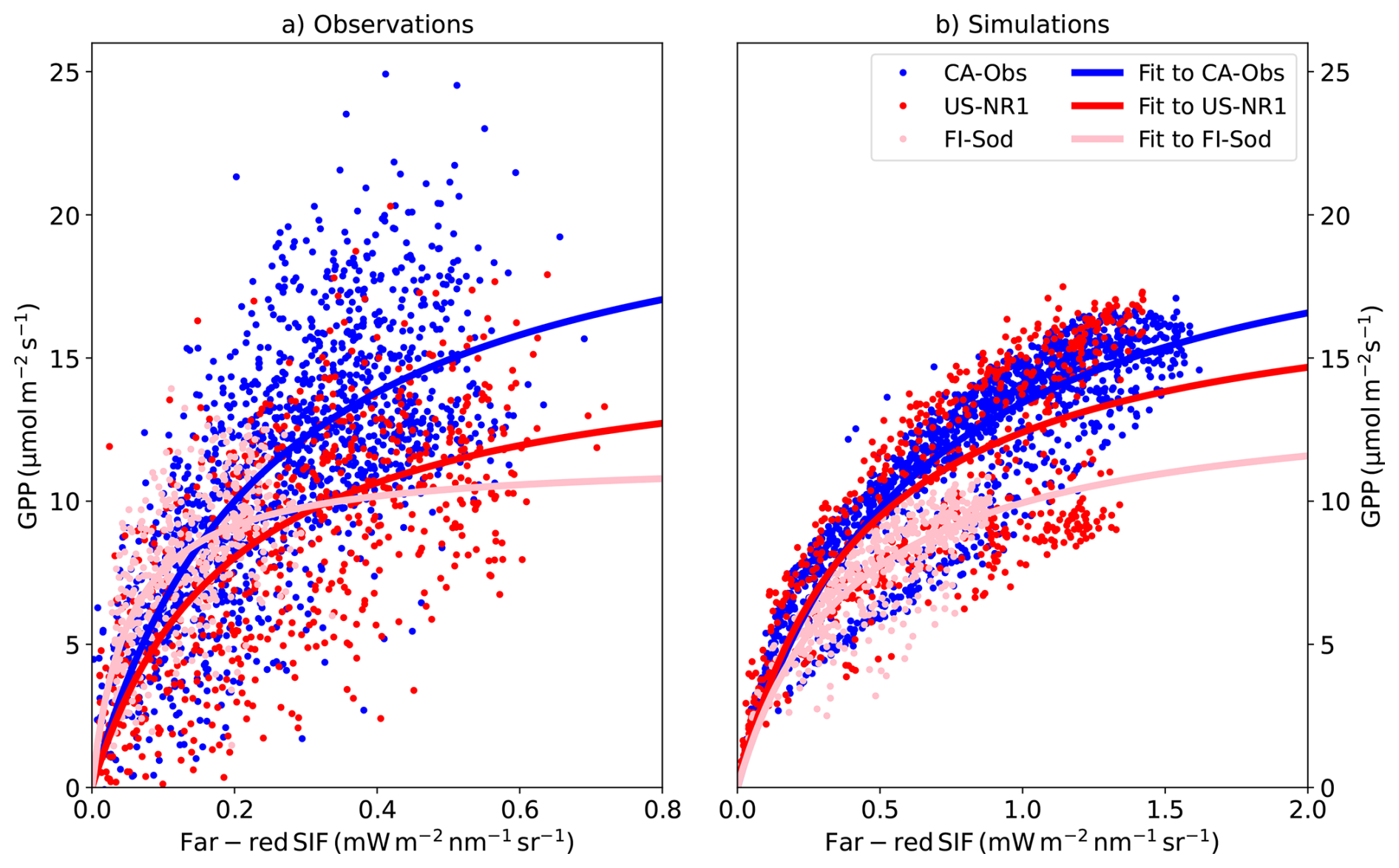
Figure 6 (a) The observed and (b) simulated GPP vs. far-red region SIF relationship at three different sites for half-hourly values for all points in June and July using the L2SM approach in the simulations. CA-Obs has half-hourly values and FI-Sod and US-NR1 hourly values. Hyperbolic fits are shown as solid lines in the figure.

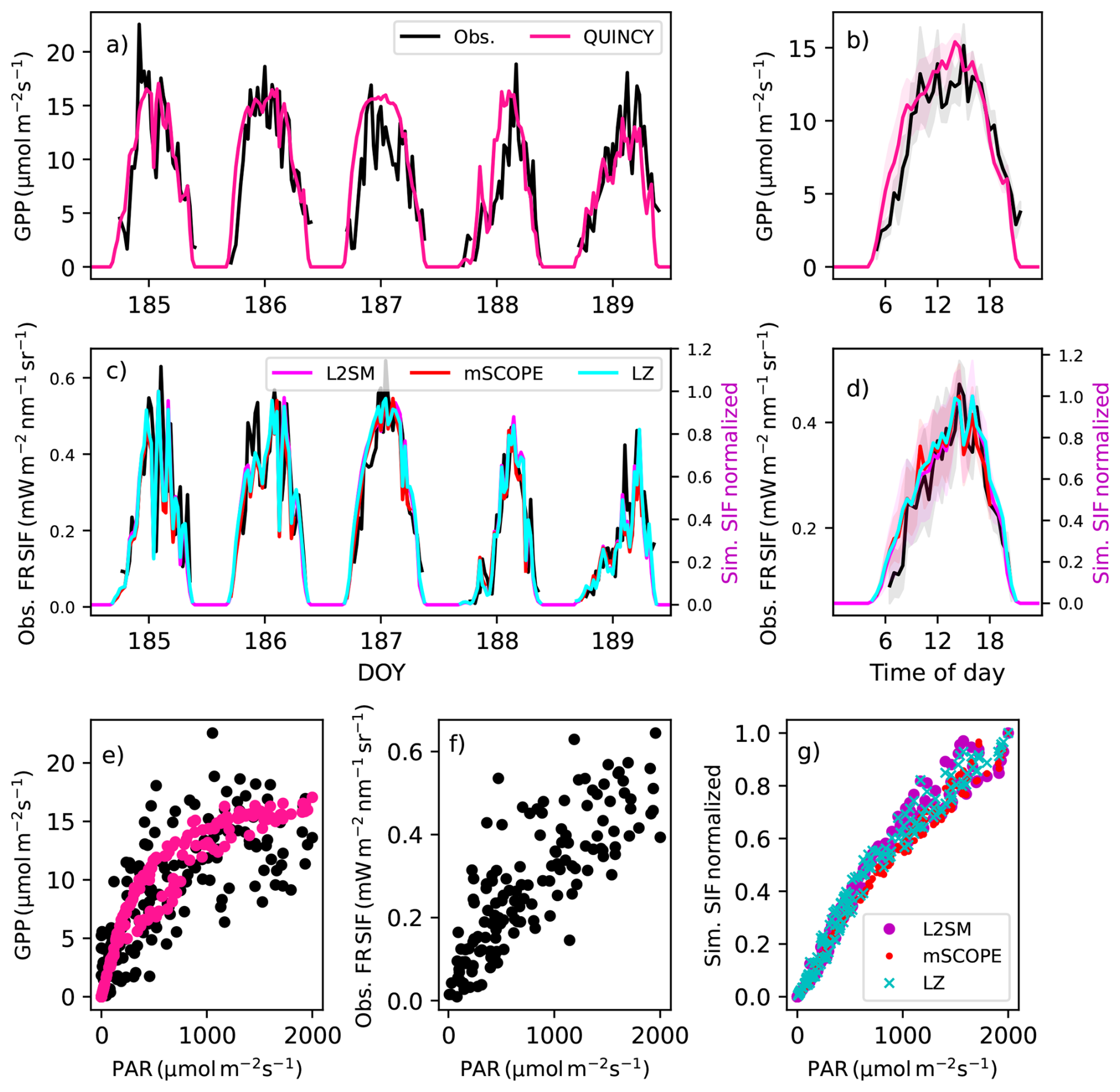
Figure 7 (a) The observed and simulated GPP and (c) far-red (denoted as FR in the figure) region SIF for days 185–189 (5–8 July 2020) and averaged over these five days (b for GPP and d for far-red region SIF) at CA-Obs. The shaded regions in b and d show the standard deviations of the averaged values. (e) The light response of the observed and simulated GPP for these five days, (f) the observed far-red region SIF and the (g) simulated far-red region SIF. The observations are in black, the simulated GPP is in pink and the simulated far-red SIF from L2SM is in magenta, from mSCOPE in red and from LZ approach in cyan. The simulated SIF values have been normalized to one.

We performed a hyperbolic fit on these relationships, determining the parameters a and b of the function $y=ax/(b+x)$ (Damm et al., 2015; Pierrat et al., 2022b). The fitted lines are shown in Fig. 6 and the fitted parameter values with their associated uncertainties are shown in Table S5. The goodness of the hyperbolic fits (Table S5) was better for the simulated GPP vs. SIF relationship than for the observed relationship (averaged over three sites r²=0.73 for the simulated and r²=0.45 for the observed.) Also, the RMSE of the fit was smaller for the simulations than for the observations at all three sites. The worst fit behaviour (in terms of r²) occurred at FI-Sod for the observations, which could reflect the fact that the GPP vs. SIF relationship was fairly linear at that site.

Due to the poorer model performance for SIF at US-NR1, the diurnal cycle during the summer was examined in more detail for all three sites. First, we calculated the r² and RMSE values for the instantaneous values over five days versus the averaged diurnal cycle values over five days. The improvement in the r² and RMSE values when moving from instantaneous to averaged values was considerable (Table 5).

Table 5 Model performance in terms of r² and RMSE for GPP and SIF in the far-red region at three sites for half-hourly values during five summer days and the averaged diurnal cycle over the five days. Calculated for half-hourly values at CA-Obs and hourly values at US-NR1 and FI-Sod. RMSE for GPP is in units $\mathrm{\mu }\mathrm{mol}{\mathrm{m}}^{-\mathrm{2}}{\mathrm{s}}^{-\mathrm{1}}$ and for SIF in ${\mathrm{Wm}}^{-\mathrm{2}}{\mathrm{s}}^{-\mathrm{1}}{\mathrm{nm}}^{-\mathrm{1}}{\mathrm{sr}}^{-\mathrm{1}}$.

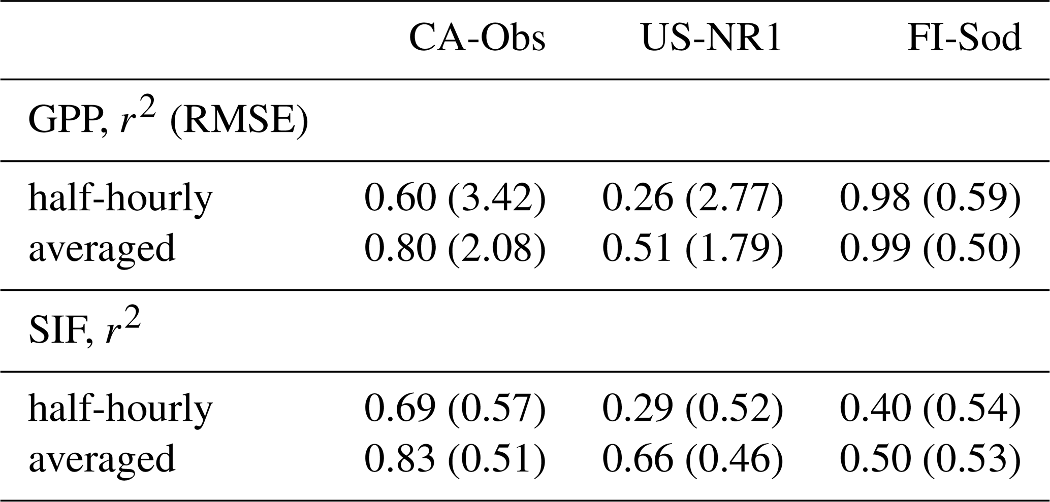
The r² values of the averaged diurnal cycle were comparable for GPP and SIF in the far-red region at CA-Obs (Table 5). On day of year (DOY) 187, the simulated GPP showed an almost sinusoidal diurnal behaviour, resulting from simulation under high irradiance conditions (Fig. 7a). The observed GPP showed more variation than the simulated GPP during the day. The light response of the observed GPP was much more scattered than that of the simulations (Fig. 7e). The simulated far-red SIF values with all the approaches were able to capture variations quite successfully on DOY 189 (Fig. 7c), when variations in radiation occurred.

At US-NR1 the model's performance was significantly lower for GPP than at the other two sites (Table 5). This remained the case even after calculating the average over five days. The light response curves of the observed GPP and SIF in the far-red region were quite scattered at this site (Fig. S14e, f). The model performed very well for GPP at Sodankylä (Table 5, Fig. S15). However, the modelled diurnal cycle of far-red SIF did not capture the observed variation (Fig. S8c, d).

3.4 Comparison of simulated SIF to satellite observations

The magnitude of the simulated SIF was larger than the tower-based observations at the two sites (Figs. 3, S6, S8). A comparison with satellite observations at CA-Obs revealed better agreement between the simulated and observed magnitudes (Fig. 8c) than with proximal sensing (Fig. 8b). In 2019, the seasonal cycle of TROPOSIF was smoother than those of the simulated SIF and PhotoSpec observations at the site. In 2020, the seasonal cycle was smoother in the PhotoSpec observations, with the simulated seasonal cycle becoming more consistent with TROPOSIF. The simulation results and the TROPOSIF are shown on different scales because the magnitude of the winter TROPOSIF observations is below zero due to the retrieval method. However, the minimum of the simulated SIF is zero, so using different scales helps to illustrate the seasonality of the two observations together. The simulations for July-August overestimated the observations by 34 %.

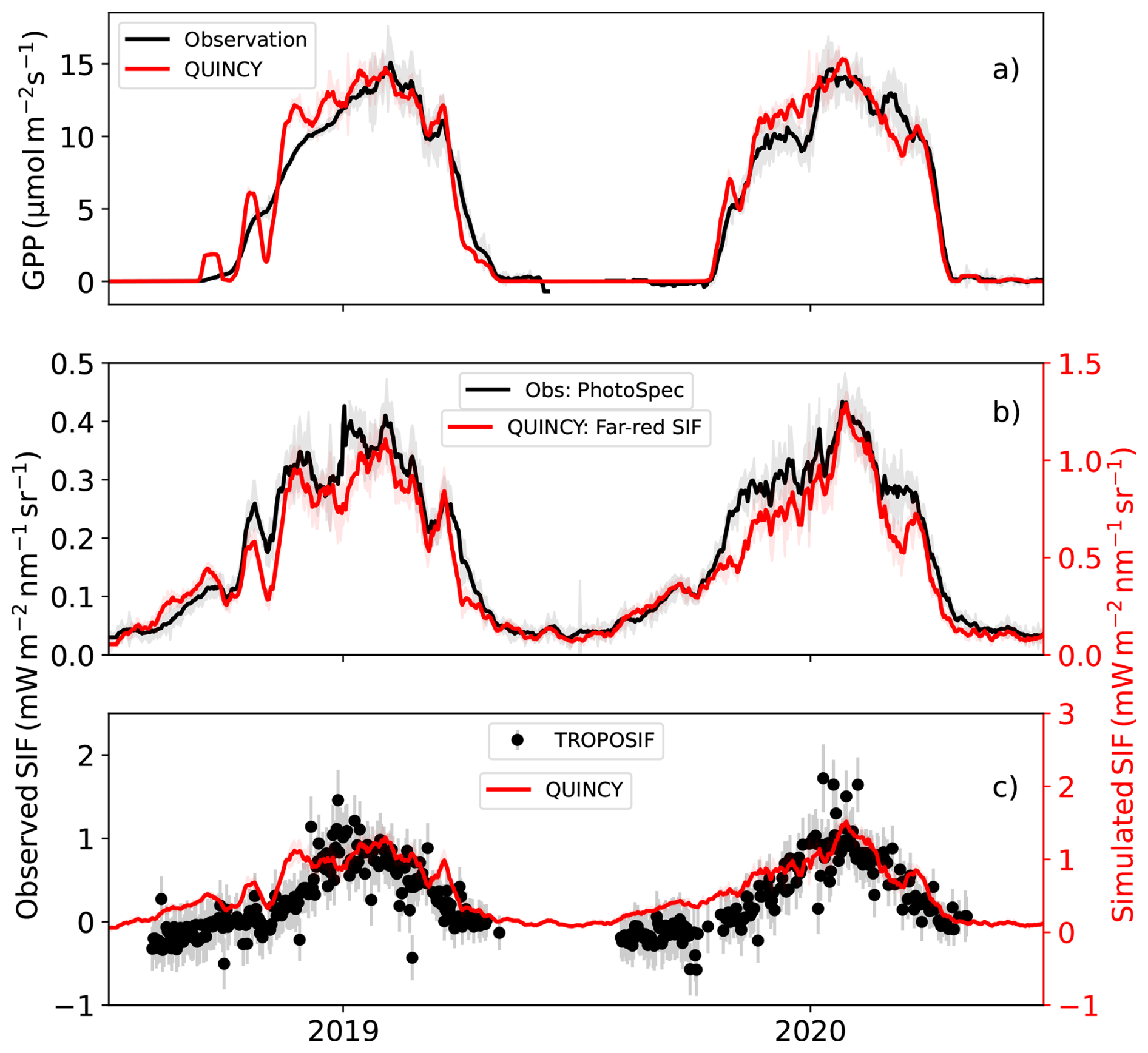
Figure 8 In (a) the observed and simulated GPP at CA-Obs, (b) near-infrared SIF from PhotoSpec observations and simulations with L2SM and (c) TROPOSIF observations and simulations with L2SM at 740 nm. The other values than TROPOSIF are averages of midday (10:00 a.m. to 01:30 p.m.) values, with standard deviation is shown as shaded areas and TROPOSIF uncertainty from the retrievals shown in error bars. TROPOSIF values are daily. All the lines for midday values have been smoothed with a 15 d long window.

At FI-Sod (Fig. S16) the TROPOSIF time series expanded also to spring, thus covering also for the period not available from the FloX observations. There was considerable variation in the TROPOSIF observations during spring (shaded region in Fig. S16, from 9 April to 17 May), and by the time the values increased for the last time in May (the vertical line in Fig. S16 showing 29 May), the observed GPP was already at higher level than in early spring. The variation in TROPOSIF and the simulated SIF followed the same pattern during the summer. Overestimation of the simulations compared to TROPOSIF observations for the July–August period was 41 %.

The performance metrics for the simulated SIF against the TROPOSIF were better at CA-Obs than at FI-Sod (Table S6). This was partly due to the fact that the sustained non-photochemical quenching was not simulated at FI-Sod. The FloX observations alone were not sufficient to assess that, as the spring was missing from them. However, as can be seen from the Fig. S16a, c, the increase in TROPOSIF should have started earlier than it did here. Despite the large differences observed in the springtime at FI-Sod, the RMSE and bias were quite similar at the two sites for the larger region (a 0.50° × 0.50° area surrounding the region). When constrained to a smaller region, the RMSE and bias worsened for both sites, but the r² increased at FI-Sod, albeit still quite small.

4 Discussion

4.1 Magnitude of the simulated SIF

All of the approaches that we tested considerably overestimated the in situ observed SIF (Table S4). The leaf level model was consistent across all our approaches. In that model, we used only the default parameters, which were held constant across all sites. The leaf level model provided the chlorophyll fluorescence yield, which was applied differently by each radiative transfer approach to obtain the top of canopy value.

Therefore, the reason for the overestimation of the SIF could originate from either the leaf level model or the radiative transfer calculation. The leaf level model provided the Ft, which was consistent with values in the literature (e.g., the original model formulation, (van der Tol et al., 2014); another modelling study for US-NR1 (Raczka et al., 2019); and site level observations (Kim et al., 2021)). However, there are other types of estimate for these values, including for some of these sites. For example, Pierrat et al. (2024) provided a higher leaf level chlorophyll fluorescence yield value from MoniPAM observations. However, the magnitude is subject to the choices made during the post-processing of the data, so it is difficult to compare the simulated value with these observations.

It is likely that the overestimation originated in the radiative transfer component of the model. Despite testing different approaches, they all resulted in an overestimation of SIF. Two approaches that included attenuation of the SIF signal inside the leaf (mSCOPE and L2SM) resulted in smaller overestimation than the approach that did not account for attenuation (LZ). Additionally, the LZ approach used here assumed black, or non-reflective, soil. Some recent developments may help to overcome this issue (Yang et al., 2025a). The simulated far-red region SIF showed lower overestimation than the simulated red region SIF. This model behaviour suggests attenuation issues in the red region. Modelling SIF is also related to modelling of absorbed PAR. At US-NR1, the simulations overestimated absorbed PAR; at the other two sites, however, the bias in aPAR was smaller (Table 4). It has been noted, that parameters related to aPAR are important for SIF modelling (Fan et al., 2025).

Overestimation of SIF has also occurred in other modelling studies of evergreen conifer forests (Li et al., 2022), and our results are close to the model average shown in a model comparison study conducted at US-NR1 (Parazoo et al., 2020). Preliminary model tests with QUINCY on other ecosystems did not reveal such significant discrepancies between the magnitude of the simulation results and in situ observations (results not shown). Therefore, it is possible that the characteristics of the in situ sampling in this type of ecosystem result in smaller SIF signals than expected. A comparison with satellite observations did not reveal such a large overestimation of the simulated SIF. It should be noted that other processes may also play a role, such as reversible NPQ. The leaf level model that we used has been parameterized for cotton (van der Tol et al., 2014). (Raczka et al., 2019) used leaf level MoniPAM observations from Hyytiälä to parameterize reversible NPQ, thereby improving the performance of their SIF model. This could be a way to improve modelling for new ecosystems.

4.2 On the choice of radiative transfer approach

First, we tested different ways of describing the radiative transfer of the SIF to determine a robust method for feasible calculations in a large-scale model. When considering the r² metric for the different approaches, we found that the simple LZ method did not perform significantly worse than the more sophisticated approaches (Tables 2, S2, S3). This justifies the rather simple approaches previously used in the radiative transfer of SIF (e.g., Lee et al., 2015; Thum et al., 2017), but it contrasts with some other studies (Li et al., 2022). The mSCOPE model performed similarly to the other approaches at all sites and often provided the most accurate estimates. However, its longer computation time (20 times longer than the other approaches in our comparison) renders it impractical for large scale applications (Li et al., 2022). The radiative transfer model in mSCOPE is based on SAIL, which was originally developed for croplands (van der Tol et al., 2009). As the radiative transfer model in QUINCY was also originally developed for croplands, neither model was designed to consider the unique characteristics of radiative transfer in the conifer forests.

The structure of the vegetation affects the observed SIF signal (Magney et al., 2019b; Sun et al., 2023a). This is something that could be addressed by including vegetation NIRv, a near-infrared reflectance, in the analysis. NIRv interacts with the canopy in a manner that is very similar to that of the far-red region SIF. Including NIRv in the analysis to help interpret the SIF signal would enable the attribution of structural effects observed in the SIF signal (Zeng et al., 2019; Dechant et al., 2022). This analysis could be conducted using in situ or spaceborne observations.

4.3 On the use of optical properties

The single leaf scattering albedo of forest plant functional types in QUINCY is based on a study by Otto et al. (2014). The values commonly used to calculate reflectance and transmittance in terrestrial biosphere models have been criticized, and some new approaches based on more extensive data have been proposed (Majasalmi and Bright, 2019). Since reflectance was also used in the calculation of the LZ approach calculation, it would also influence these results. The assumption of equal reflectance and transmittance in QUINCY is debatable and could be further developed, as discussed in Majasalmi and Bright (2019). Using only two radiative bands (visible and near infrared) may introduce biases in the results at certain wavelengths.

The L2SM and the LZ approaches require SIF spectra for unit conversion from modelled to observed units (see Sect. 2.6). For the LZ approach, we used spectra measured in a Finnish Scots pine forest. To extend this approach to other PFTs, different measured SIF spectra would need to be used. This approach is limited in terms of generalizability because these spectra differ between species (Liu et al., 2025; Magney et al., 2017). Therefore, using a single spectrum for a PFT may introduce uncertainties. Furthermore, the spectral shape of SIF emission changes under stress conditions. For example, photosystems I and II respond differently to stress (Magney et al., 2019a), which will further limit our approach, and require careful investigation of the stress effects. For the L2SM approach we used a theoretical estimate of the in vivo spectrum. Further testing with observed in vivo spectra would also improve this approach. The simulated clumping index at the FI-Sod (Fig. S1) was close to the observed estimates (Chen et al., 2005; Schraik et al., 2023). The seasonal cycle was consistent with the observed increase in the clumping index with increasing solar zenith angle (Chen and Cihlar, 1995).

4.4 Uncertainties in the observations

Using the Fraunhofer line method with PhotoSpec instruments makes the measurement less susceptible to atmospheric attenuation than using the oxygen lines with FloX. At FI-Sod, the distance from the soil to the FloX instrument was around 19–20 m, and the distance to the canopy was shorter. Therefore, the measurement distance was less than 20 m, which is the threshold at which the data must be corrected for atmospheric effects (Sabater et al., 2018; van der Tol et al., 2023). FI-Sod has a sparser canopy than the other sites, meaning the footprint of the observing optical fiber is susceptible to environmental influences other than the canopy, such as the understory. The nearly linear relationship between GPP and SIF in the observations may indicate understory contribution (Fig. 6a).

The measurements that we used have several sources of uncertainty. The tower SIF observations are relatively new observations and are subject to uncertainties relating to instrumentation, the retrieval method, and the spatial matching of the optical and flux footprints (Buman et al., 2022; Cendrero-Mateo et al., 2019; Pacheco-Labrador et al., 2019). Our results showed that averaging could be useful for the model evaluation. The eddy covariance observations are subject to uncertainty due to the measuring equipment, the heterogeneity of the footprint, and the stochastic nature of turbulence (Richardson et al., 2006). Gap-filling introduces further uncertainties to the data (Vekuri et al., 2025).

Comparing the satellite observations to a site level observations introduces several uncertainties. The fact that the TROPOSIF estimates remain close to zero by the end of May at FI-Sod, despite the GPP levels advancing towards summer levels, indicates that these observations must be treated with caution. Clouds make interpreting the signal more challenging, which is why we applied the strict cloud filtering criterion recommended for this type of study. There is a large mismatch in scale between the satellite and flux tower observations. However, constraining the region did not improve the modelling results. This may be because having more data points helps to smooth out the random errors in the satellite observations. When only the pixels where the site was located were selected from the satellite retrievals, there were so few data points that no significant seasonal cycle could be detected (data not shown). Data aggregation for TROPOSIF involves averaging over several viewing geometries because the viewing angle varies due to the wide swath. This introduces additional uncertainty to the data. Using the “daily corrected” values of TROPOSIF would help limit the influence of the uneven number of observations on each day. The land cover classes within the TROPOSIF product that are derived from the MODIS product have issues in the high latitudes, which is a known issue (Liang et al., 2019). However, the land cover class does not affect the retrieved SIF because it is only used to identify water bodies and glaciers. Overall uncertainty in the TROPOSIF product has been found to be ∼ 0.50 ${\mathrm{Wm}}^{-\mathrm{2}}{\mathrm{s}}^{-\mathrm{1}}{\mathrm{nm}}^{-\mathrm{1}}{\mathrm{sr}}^{-\mathrm{1}}$ (Guanter et al., 2021; Du et al., 2023), which emphasizes that the low values during the shoulder seasons for these northern sites are highly uncertain.

4.5 Model uncertainties and limitations

Our model only simulates one plant functional type per site, and it is also horizontally homogeneous. Therefore, the influence of the understory is disregarded, even though it may be relevant. A study by Li et al. (2022) found that including clumping in their model significantly improved SIF modeling in CLM compared to simulations without clumping. Failing to consider clumping can lead to significant errors in SIF modelling (Zeng et al., 2020). QUINCY describes clumping in a relatively simple way. There is potentially room for improvement in SIF modelling if clumping were also included in the radiative transfer of SIF, e.g. in L2SM. In coniferous forests, the challenge is that the clumping of the canopy exposes more ground vegetation visible to optical measurements, affecting the remotely sensed signal (Gopalakrishnan et al., 2023).

Compared to the simulated GPP, the observed GPP showed more variation on a subdaily scale at the sites (Figs. 7, S14, S15). This variation may be due to canopy shading, understorey vegetation and turbulence conditions. The lower performance at CA-Obs in the morning for the simulated SIF may be due to the sun-view geometry and the 3D structure of the canopy, which casts shadows within the spectroradiometer's measurement footprint. These shadows were not reproduced by 1D radiative transfer models. At FI-Sod shadows could also contribute to the discrepancy between FloX observations and simulations (Fig. S15c, d). Designing an observation that excludes the shadow effects would be very challenging at such high latitudes, where the days are very long in the summer. More rigorous modelling tools, such as a 3D description of forest structure, would be required to account for these effects. In reality, directional effects also influence the observed optical signal, but our approach did not account for them (Hilker et al., 2008b, a). A comparison of simulated and observation based estimates of aPAR from the FloX and PAR sensors revealed that the model's inability to capture certain dynamics observed by the FloX box may be due to its small footprint.

The scatter of the observed SIF against the observed GPP values, as well as the fact that model was unable to fully capture this behaviour (Fig. 6), raises questions about the accuracy of the simulated SIF provides reasonable results in water-stressed conditions (an example of dry period shown at FI-Sod in Thum et al., 2007). However, due to the scattered nature of the SIF observations, having a more comprehensive dataset than that used in this study would be helpful.

4.6 Role of sustained NPQ

Our results showed a strong influence of sustained NPQ at these sites, where the plants cannot use the energy of the incoming radiation due to temperature constraints and winter dormancy (see also Pierrat et al., 2024). In general, simulating NPQ has been a challenge to the modelling community, as it is comprises of many processes (Zaks et al., 2013), and active measurements have been required to quantify it. However, recent advances in the use of spectral imaging of xanthophyll cycle pigments potentially enable quantifying NPQ also from the optical observations (Pescador‐Dionisio et al., 2025; Van Wittenberghe et al., 2024), thus making remote sensing of NPQ feasible. Some studies have also combined vegetation indices to assist with the parameterization of NPQ (Jiang et al., 2023). Some new parameterizations for NPQ based on site-level observations have also become available (Martini et al., 2022).

The current results showed that the formulation that was successful at other sites likely caused a too early increase in simulated SIF in spring at FI-Sod, when compared with satellite observations (Fig. S16). The colder temperature and light regime at high latitudes may cause the FI-Sod to exhibit different dormancy levels and coping mechanisms for winter conditions compared to sites in North America. A study of a South Korean evergreen coniferous forest showed that the observed chlorophyll fluorescence yield (Φ_F) was lower at low temperatures than our parameterization allowed (Fig. S12). Therefore, it is likely that the parameterization could be improved for the FI-Sod, while still maintaining realistic values for Φ_F. Although a similar parameterization for GPP based on the state of acclimation was successful across sites, the same could not be said for a parameterization based on similar principles for sustained NPQ. This may be due to the closer link between ChlF and changes in the pigment pool than between GPP and the pigment pool (Kim et al., 2021). The cold protection mechanisms of conifers are complex and include additionally changes in the absorption cross-section of the antenna complexes, as well as downregulation of photosystem II activity, accompanied by the transfer of energy from photosystem II to photosystem I (Bag et al., 2020). Previous studies have demonstrated that the ratio of GPP to SIF fluctuates at low temperatures (Chen et al., 2022, 2025). It is important to model the dynamics of this behaviour in order to understand the coupling between GPP and SIF.

A recent study combining PAM observations worldwide evaluated the photosynthetic capacity of photosystem II (Neri et al., 2024). The study showed that this capacity depends more on the temperature regime of the environment where the vegetation grows than on the species of plant. The study also quantified this dependence. The ultimate goal is to obtain a sufficiently general parameterization for the entire coniferous evergreen forest region, using the results of Neri et al. (2024). Using the same model for photosynthesis and ChlF (Johnson and Berry, 2021) could potentially circumvent this problem. However, the current photosynthesis parameters in QUINCY are directly influenced by nitrogen content and leaf chlorophyll content is also closely coupled to photosynthesis (Thum et al., 2025). Leaf chlorophyll content could be useful as a metric related to nitrogen cycling in model evaluation (Miinalainen et al., 2025). This is a much-needed metric (Kou-Giesbrecht et al., 2023). Additionally, the amount of leaf chlorophyll influences how much of the SIF emitted from leaves that is attenuated in the canopy within the visible spectrum. Therefore, including both leaf chlorophyll and SIF in a model such as QUINCY would be beneficial for understanding Earth system processes and their temporal variations. The amount of chlorophyll in leaves also affects the shape of the SIF spectrum. As we used a fixed SIF spectrum to convert from the total SIF flux to SIF at a given wavelength (Magney et al., 2019b), this topic could benefit from some further investigation.

5 Conclusions

We have implemented chlorophyll fluorescence into the QUINCY model and tested different canopy transfer approaches of the SIF signal. On a seasonal scale, many of the approaches performed similarly, and did not show clear differences in performance when looking at day-to-day variation and the ability to simulate different times of day. The magnitude of the tower-based SIF observations was greatly overestimated in the simulations, but the timing and seasonality were captured successfully. Of the approaches studied, L2SM showed consistent performance across the sites and is computationally feasible to implement in a large-scale model. We hypothesize that the consistent overestimation might arise from the misrepresentation of conifer needles and canopy. The leaf plate-theory-based radiative transfer models does not reproduce the cylindrical structure of needles. At the same time, the 1D canopy radiative models do not incorporate the strong clumping of conifer needles. However, no fluorescence emission has been implemented in needle-like leaf radiative transfer models, and 3D canopy transfer modules are too computationally demanding for TBMs. Thus, simpler modeling solutions should be explored to improve the representation of fluorescence emission in conifer forests, with the help of proximal sensing measurements.

Sustained NPQ was relevant in decoupling the simulated SIF from the observed absorbed PAR and the same parameterization improved model performance at the North American sites but appeared less suitable at the Finnish site. This process is likely linked to the air temperature regime of the sites. The TROPOSIF product was able to capture the low spring values observed at CA-Obs and could therefore probably serve as additional data when implementing the parameterization of sustained NPQ in a global model. However, for more northern site FI-Sod the amount of points in spring was sparse and an increase in TROPOSIF occurred later than for GPP. Use of TROPOSIF observations additionally in model evaluation and development seems feasible, given that the springtime behaviour seems to follow better site level observations of SIF than absorbed PAR.

The next step of this work will be to extend it to other ecosystems, using both in situ and satellite observations as evaluation data. Together with QUINCY's diagnostic leaf chlorophyll content, a variable which can be observed from space, this work brings QUINCY closer to being a tool for comprehensive analysis of biogeochemical cycles.