Data-based estimates of ocean carbon uptake biased high from neglect of submonthly atmospheric pressure variability

Current estimates of the global ocean carbon sink based on measurements of CO₂ fugacity are inconsistent with those obtained from global ocean biogeochemistry models. Here we investigate how this gap might change by more fully accounting for submonthly variability in observation-based estimates, a step closer to the roughly hourly frequencies used in models. While these data-based estimates use hourly to 6-hourly wind speeds to compute the air-sea CO₂ flux, other input variables are available only at monthly resolution. Thus, they neglect high-frequency variability in key variables such as atmospheric pressure associated with synoptic events such as storms. To evaluate this error, we compare flux estimates from observational data sets with different temporal resolutions. Accounting for hourly variations in atmospheric pressure and daily variations in sea surface temperature, a data-based approach reduces the estimated global carbon uptake by 0.12 Pg C yr⁻¹, closing 25 % of the average gap between observation-based and model estimates. This reduction results from proper accounting of the covariance between wind speed and atmospheric pressure, particularly in the southern extratropics.

1 Introduction

The ocean absorbs one-fourth of anthropogenic CO₂ emissions, playing a major role in the global carbon cycle. It is estimated to have absorbed 2.9 Pg C yr⁻¹ of anthropogenic carbon during 2014–2023 based on the Global Carbon Budget (GCB, Friedlingstein et al., 2025). But this average value comes with a spread of more than 1 Pg C yr⁻¹ between the lowest and highest estimates. The GCB is updated annually to reflect the evolution in the data and methods used to obtain the latest estimates of global carbon emissions and carbon storage in different reservoirs (sinks). Its ocean estimate relies on two different approaches.

The first approach uses global ocean biogeochemistry models (GOBMs), each of which couples a global-scale, general ocean circulation model to an ocean carbon cycle component. GOBMs simulate ocean transport of dissolved inorganic carbon (DIC) and total alkalinity (Alk), from which is calculated surface ocean CO₂ fugacity (fCO_2 sea), a variable nearly identical to the ocean partial pressure of CO₂ (pCO_2 sea). From that, the models compute the difference relative to the atmospheric CO₂ fugacity (fCO_2 atm), multiplying that difference by a gas transfer velocity times the solubility to compute the air-sea CO₂ flux. The simulated air-sea CO₂ flux is affected by multiple physical atmospheric variables since the gas transfer velocity is often parameterized as a quadratic function of wind speed and fCO_2 atm depends in part on atmospheric pressure and vapor pressure. GOBMs are typically forced by atmospheric reanalyses having hourly to 6-hourly timesteps. Nonetheless, simulated ocean uptake of anthropogenic carbon in GOBMs is only weakly sensitive to uncertainties in the gas transfer velocity. For example, a doubling of the gas transfer velocity led to only a 9 % increase in simulated ocean uptake of anthropogenic carbon (Sarmiento et al., 1992). The extra CO₂ added to the ocean from enhanced gas exchange is not transported away from the surface quickly enough, thus increasing the simulated fCO_2 sea and reducing the change in the air-sea flux, a key feedback inherent not only in models but also in the real ocean. While models have their own problems, such as biases in simulated circulation fields, they are insensitive to the magnitude of the gas transfer velocity.

The second approach uses observation-based products for fCO_2 sea rather than modeled fields. These data products rely on millions of in situ measurements of fCO_2 sea archived in the Surface Ocean CO₂ Atlas (SOCAT, Bakker et al., 2016). Many groups have used this unevenly spaced data to produce evenly spaced gridded data products, mapping it typically to a 1° × 1° grid with monthly resolution and filling missing grid cells based on a series of global predictors, e.g., sea surface temperature and mixed-layer depth, obtained from satellite products and atmospheric and oceanic reanalyses (Landschützer et al., 2016; Rödenbeck et al., 2022; Chau et al., 2024 Watson et al., 2020; Zeng et al., 2022; Iida et al., 2021; Gregor et al., 2024; Gloege et al., 2022; Gregor et al., 2019). Using observed rather than simulated fCO_2 sea is an advantage since it reflects the real ocean's air-sea interaction. But it comes with a disadvantage: the data-based approach cannot benefit from the previously mentioned feedback between the flux and fCO_2 sea. Thus, compared to the GOBMs, data-based estimates of air-sea CO₂ fluxes are more sensitive to errors in the bulk flux parameterization, with associated uncertainties scaling proportionally to the imposed gas transfer velocity (Gloege and Eisaman, 2025; Jersild and Landschützer, 2024).

It is estimated that the ensemble mean 1σ uncertainty for the 10 models is 0.5 Pg C yr⁻¹ while that for the 8 data products is 0.6–0.7 Pg C yr⁻¹ considering both random and systematic uncertainties (Friedlingstein et al., 2025; Ford et al., 2024). Moreover, there is a systematic discrepancy between the two approaches, where the average sink from data-based products is 0.5 Pg C yr⁻¹ larger than that from GOBMs. Friedlingstein et al. (2025) suggest a possible 10 %–20 % underestimate from the GOBMs for the ocean uptake of anthropogenic carbon owing to several potential problems: an overestimated Revelle factor, salinity biases in the Southern Ocean, an underestimated penetration of carbon into the ocean interior from weak vertical mixing and transport, and a delayed beginning for the anthropogenic perturbation, after the actual start of the industrial era (see Bronselaer et al., 2017; Terhaar et al., 2022, 2024).

Other potential sources of model-data discrepancy come from the data-based approach. First, there is the 0.65 ± 0.15 Pg C yr⁻¹ that must be added to the data-based estimates to back calculate the anthropogenic carbon flux from the total flux by removing the global effect of the net preindustrial outgassing driven by the natural imbalance between riverine input and sediment loss of carbon (Aumont et al., 2001; Regnier et al., 2022), as discussed by DeVries et al. (2023), Pérez et al. (2024) and Planchat et al. (2025). Another important source of uncertainty is the sparsity of SOCAT measurements in some key regions such as the Southern Ocean (Hauck et al., 2020, 2023; Ford et al., 2024). Finally, discrepancies may also stem from the very different temporal resolutions of the two approaches. While GOBMs compute air-sea CO₂ fluxes with a time step on the order of an hour, the data-based products used in GCB 2024 generally rely on monthly averaged variables. Fortunately, the data-based products do account for the effect of submonthly wind-speed variance by using monthly means of the square of observed 1- to 6-hourly wind speed when computing the gas transfer velocity. But they neglect nonlinearities stemming from submonthly variability of other physical drivers, including atmospheric pressure, sea surface temperature, and sea surface salinity.

To address this limitation, Gregor et al. (2024) developed a higher-frequency data product computing the CO₂ flux with 8 d temporal resolution, but they also showed its use had minimal effect on the resulting global sink estimate. Unfortunately, an 8 d frequency still does not resolve intense meteorological events, such as tropical cyclones and extratropical storms, which drive variations in atmospheric and oceanic variables on shorter time scales. Previous case studies have shown that tropical cyclones can cause substantial regional ocean carbon uptake (Gregor et al., 2024) or outgassing (Bates et al., 1998; Huang and Imberger, 2010), depending largely on the initial sign of the CO₂ fugacity difference at the air-sea interface. Yet the resulting global contribution of tropical cyclones to the ocean carbon sink is negligible (Lévy et al., 2012) because they mostly occur in regions with weak air-sea differences in fCO₂ and because they increase CO₂ fluxes both into and out of the ocean, nearly canceling one another. Extratropical studies with data from floats and gliders indicate that storms in the Southern Ocean can provoke outgassing anomalies over 1–3 d, driven by concomitant variations in wind speed, atmospheric pressure, and DIC concentrations (Carranza et al., 2024; Nicholson et al., 2022). The Argo float-based estimates suggest that Southern Ocean storms may reduce the global carbon sink by up to 0.057 Pg C yr⁻¹ (Carranza et al., 2024). But storms represent only a part of the submonthly phenomena. It remains uncertain how high-frequency variability, if it were properly accounted for in data-based approaches, would affect resulting estimates of the air-sea CO₂ flux at the global scale.

Although submonthly and particularly synoptic variability of ocean biogeochemical variables (fCO₂, DIC …) cannot yet be constrained at the global scale due to the scarcity of observations, such is not the case for physical variables including not only wind speed but also atmospheric pressure, sea surface temperature and salinity. Here we ask how much this submonthly variability might affect observation-based estimates of the global ocean carbon sink, particularly in mid-latitudes where storms induce outgassing through simultaneous decreases in atmospheric pressure and increases in wind speed. Our aim is to quantify the importance of this effect, identifying the responsible non-linearities between variables and the regions where they dominate.

2 Methods

2.1 CO₂ flux calculations

Consistent with the GCB, our data-based air-sea CO₂ flux F is computed as

$$\begin{array}{}\text{(1)}& F=k_{\mathrm{660}}\left(u\right)A(T,S)\left(f{\mathrm{CO}}_{\mathrm{2}\mathrm{atm}}-f{\mathrm{CO}}_{\mathrm{2}\mathrm{sea}}\right).\end{array}$$

where k₆₆₀ is the gas transfer (piston) velocity at 20 °C, fCO_2 atm and fCO_2 sea are the fugacities of CO₂ in the atmosphere and the ocean, and $A=K_{\mathrm{0}}(T,S){\left(\frac{Sc\left(T\right)}{\mathrm{660}}\right)}^{\frac{-\mathrm{1}}{\mathrm{2}}}$ with K₀ being the solubility of CO₂ in seawater computed from the sea surface temperature (T) and salinity (S) (Weiss, 1974), and the Schmidt number (Sc) ratio is used to adjust the wind-speed formulation for gases other than CO₂ and for temperatures other than 20 °C (Wanninkhof, 2014). Positive fluxes indicate an air-to-sea CO₂ flux. The k₆₆₀ is calculated using a quadratic function of wind speed k₆₆₀=au² (Wanninkhof, 1992), where u is the wind speed at 10 m. As for a, it is an empirical scaling constant adjusted for each wind dataset so that the corresponding global value of k (i.e., k₆₆₀ normalized to different temperatures with the Schmidt number ratio above) averages 16.5 cm h⁻¹ over the ice-free ocean as derived from the observed global bomb ¹⁴C inventory (Naegler, 2009). Since it is based on the real ocean inventory of bomb ¹⁴C, this scaling approach should inherently account for the effects of submonthly variability of all variables that affect the gas transfer velocity; however there is a 20 % uncertainty associated with the bomb ¹⁴C inventory and thus k.

The CO₂ fugacity in the atmosphere, fCO_2 atm, is the partial pressure of CO₂ corrected for the non-ideal behaviour of the gas. The fCO_2 atm, (in µatm) is computed from the dry-air mixing ratio (or mole fraction) of CO₂ (in ppm), as follows

$$\begin{array}{}\text{(2)}& f{\mathrm{CO}}_{\mathrm{2}\mathrm{atm}}={\mathit{\varphi }}_{{\mathrm{CO}}_{\mathrm{2}}}\left(P_{\mathrm{atm}},T\right)X_{{\mathrm{CO}}_{\mathrm{2}}}\left(P_{\mathrm{atm}}-P_{\mathrm{vap}}\left(T,S\right)\right)\end{array}$$

where ${\mathit{\varphi }}_{{\mathrm{CO}}_{\mathrm{2}}}$ is the fugacity coefficient from Weiss (1974), $X_{{\mathrm{CO}}_{\mathrm{2}}}$ is the CO₂ mole fraction in dry air (ppm), P_atm is the surface atmospheric pressure (atm), and P_vap is the partial pressure of water vapor (atm) from Weiss and Price (1980), an empirical function of T and S assuming that the air is fully saturated (100 % humidity) just above the air-sea interface.

For simplicity, in contrast with GCB data-based product, our oceanic fugacity fCO_2 sea is not from an ocean fCO₂ observation product but is instead computed from gridded products of T, S, DIC, Alk, and total inorganic phosphorus and silicon concentrations ([P] and [Si]) using mocsy (Orr and Epitalon, 2015). This simplification enables us to evaluate the impact of submonthly variability of T and S on fCO_2 sea while maintaining the basic GCB data-based approach.

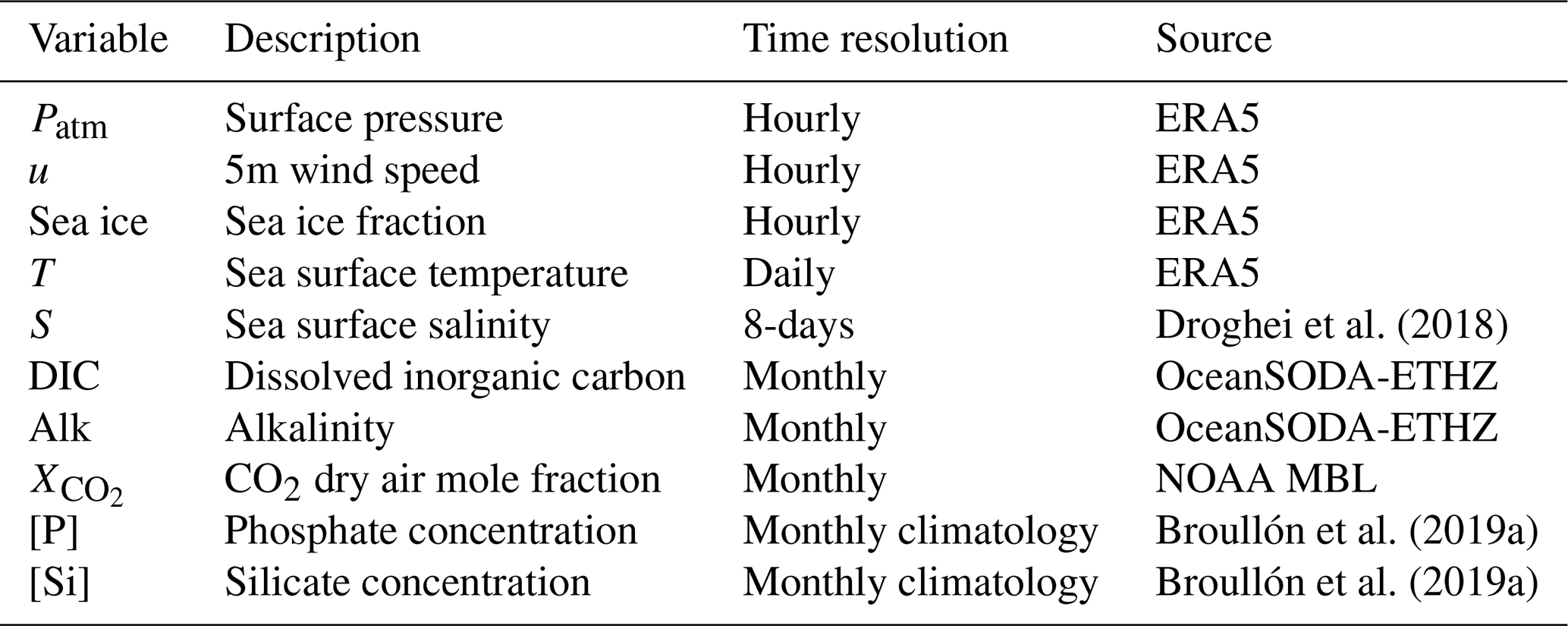
We use hourly fields of wind speed u and surface pressure P_atm, and daily fields of sea surface temperature T and sea ice concentration from the fifth generation ECMWF reanalysis (ERA5, Hersbach et al., 2020) at 0.25° × 0.25° spatial resolution. In the gas transfer velocity formulation, the empirical scaling constant a is taken to be 0.271 as computed for the ERA5 wind speed field by Fay et al. (2021). We also use the bulk daily sea surface temperature rather than the hourly sea-surface skin temperature to be consistent with current GCB data-based estimates. All but one of those estimates use bulk sea surface temperature. Thus, we do not include effects of diurnal warming and cool skin that have been addressed in previous studies (Watson et al., 2020; Dong et al., 2022; Bellenger et al., 2023). Sea-surface salinity S is taken from the Multi Observation Global Ocean Sea Surface Salinity and Sea Surface Density dataset (Droghei et al., 2018) with 0.25° × 0.25° spatial resolution and 8 d temporal resolution. Atmospheric CO₂ dry air mole fraction $X_{{\mathrm{CO}}_{\mathrm{2}}}$ is from the NOAA Greenhouse Gas Marine Boundary Layer Reference (Lan et al., 2023), provided as 4.5° latitudinal bands at a temporal resolution of ∼ 8 d. For $X_{{\mathrm{CO}}_{\mathrm{2}}}$, we computed its monthly means because of the limited observational network used to produce this global data set, thus leaving the impact of its submonthly variability for future studies. Fields of DIC and Alk are from OceanSODA-ETHZ (Gregor and Gruber, 2021), which has 1° × 1° spatial resolution and monthly temporal resolution. Fields of [P] and [Si] are from a monthly climatology (Broullón et al., 2019a) derived from the 2013 World Ocean Atlas dataset (Boyer et al., 2013), also on a 1° × 1° grid. Before computing fluxes, all datasets are regridded to a common 0.25° × 0.25° grid using bilinear interpolation. Air-sea CO₂ fluxes are calculated from 2009 to 2018 and, for simplicity, only for latitudes between 60° S and 60° N, thus avoiding most sea-ice covered areas. Calculations consider only the time steps when grid cells have no ice cover. Regions poleward of 60° contribute only marginally to the global sink (Takahashi et al., 2009). Table 1 summarizes the data used in this study.

Table 1 Sources of all datasets used in this study.

To study the sensitivity of the global ocean carbon sink to the submonthly variability that is neglected in GCB data-based products, we computed two estimates: (1) our reference, using monthly averages for all variables except for wind speed, which as in GCB already accounts for submonthly wind speed variance; and (2) our test case, using instead higher temporal resolution data for atmospheric pressure, sea-surface temperature, and sea surface salinity. Consistent with the temporal resolution of GCB 2024 data products, the reference flux F_ref is calculated using the monthly mean of the squared wind speed computed from hourly data of $\stackrel{\mathrm{‾}}{u^{\mathrm{2}}}$ and monthly means of the other variables:

$$\begin{array}{}\text{(3)}& \begin{array}{rl}{F}_{\mathrm{ref}}& =a\cdot \stackrel{\mathrm{‾}}{u^{\mathrm{2}}}\cdot A\left(\stackrel{\mathrm{‾}}{T},\stackrel{\mathrm{‾}}{S}\right)\\ & \cdot \mathrm{\Delta }f{\mathrm{CO}}_{\mathrm{2}}\left(\stackrel{\mathrm{‾}}{P_{\mathrm{atm}}},\stackrel{\mathrm{‾}}{T},\stackrel{\mathrm{‾}}{S},\stackrel{\mathrm{‾}}{X_{{\mathrm{CO}}_{\mathrm{2}}}},\stackrel{\mathrm{‾}}{\mathrm{DIC}},\stackrel{\mathrm{‾}}{\mathrm{Alk}},{\stackrel{\mathrm{‾}}{\left[\mathrm{P}\right]}}^{\mathrm{c}},{\stackrel{\mathrm{‾}}{\left[\mathrm{Si}\right]}}^{\mathrm{c}}\right)\end{array}\end{array}$$

The overbar denotes a monthly mean, while the appended c superscript indicates a climatological monthly mean. The high-frequency flux F_h is calculated hourly using each variable at its highest available temporal resolution (hourly u and P_atm, daily T, 8-daily S, and monthly for all others). We compare F_ref to $\stackrel{\mathrm{‾}}{F_{\mathrm{h}}}$, the monthly mean of F_h:

$$\begin{array}{}\text{(4)}& \stackrel{\mathrm{‾}}{F_{\mathrm{h}}}=\stackrel{\mathrm{‾}}{a\cdot u^{\mathrm{2}}\cdot A\left(T,S\right)\cdot \mathrm{\Delta }f{\mathrm{CO}}_{\mathrm{2}}\left(P_{\mathrm{atm}},T,S,\stackrel{\mathrm{‾}}{X_{{\mathrm{CO}}_{\mathrm{2}}}},\stackrel{\mathrm{‾}}{\mathrm{DIC}},\stackrel{\mathrm{‾}}{\mathrm{Alk}},{\stackrel{\mathrm{‾}}{\left[\mathrm{P}\right]}}^{\mathrm{c}},{\stackrel{\mathrm{‾}}{\left[\mathrm{Si}\right]}}^{\mathrm{c}}\right)}\end{array}$$

To further assess the causes of differences, we also compare F_ref and $\stackrel{\mathrm{‾}}{F_{\mathrm{h}}}$ to the monthly averages of two intermediate air-sea CO₂ fluxes: (1) $\stackrel{\mathrm{‾}}{F_P}$ which is computed like $\stackrel{\mathrm{‾}}{F_{\mathrm{h}}}$ but using hourly P and monthly T and S and (2) $\stackrel{\mathrm{‾}}{F_{P,T}}$, which is computed using hourly P_atm, daily T, and monthly S. Then the difference $\stackrel{\mathrm{‾}}{F_P}-F_{\mathrm{ref}}$ shows the importance of taking into account high-frequency variability of P_atm. Another difference $\stackrel{\mathrm{‾}}{F_{P,T}}-\stackrel{\mathrm{‾}}{F_P}$ reflects the importance of taking into account daily T, while $\stackrel{\mathrm{‾}}{F_{\mathrm{h}}}-\stackrel{\mathrm{‾}}{F_{P,T}}$ shows the impact of submonthly variations of S.

Finally, the corresponding global ocean sinks of anthropogenic carbon S_h and S_ref are obtained by spatially integrating the air-sea CO₂ flux (between 60° S and 60° N) and correcting for preindustrial outgassing by subtracting the global $S_{\mathrm{river}}=\mathrm{0.65}\pm \mathrm{0.15}$ Pg C yr⁻¹ (Regnier et al., 2022).

We consider that the differences $\stackrel{\mathrm{‾}}{F_{\mathrm{h}}}-F_{\mathrm{ref}}$ and S_h−S_ref are statistically significant only if they differ from 0 at the 99 % level using Student's t-test.

2.2 Reynolds decomposition

To investigate the non-linearities between high-frequency variations of the variables that are responsible for differences between F_ref and $\stackrel{\mathrm{‾}}{F_{\mathrm{h}}}$, a Reynolds decomposition is used with respect to u and $\mathrm{\Delta }=f{\mathrm{CO}}_{\mathrm{2}\mathrm{atm}}-f{\mathrm{CO}}_{\mathrm{2}\mathrm{sea}}$ for each month from 2009 to 2018, assuming that the solubility and Schmidt number variations cancel out to give $A=\stackrel{\mathrm{‾}}{A}$ (Etcheto et Merlivat, 1988), an assumption good to within 5 % locally (Wanninkhof, 2014):

$$\begin{array}{}\text{(5)}& \begin{array}{rl}{F}_{\mathrm{h}}& =aA{\stackrel{\mathrm{‾}}{u}}^{\mathrm{2}}\stackrel{\mathrm{‾}}{\mathrm{\Delta }}+aA{\left(u^{\prime }\right)}^{\mathrm{2}}\stackrel{\mathrm{‾}}{\mathrm{\Delta }}+\mathrm{2}aA\stackrel{\mathrm{‾}}{u}{u}^{\prime }{\mathrm{\Delta }}^{\prime }\\ & +aA{\left(u^{\prime }\right)}^{\mathrm{2}}{\mathrm{\Delta }}^{\prime }+aA{\stackrel{\mathrm{‾}}{u}}^{\mathrm{2}}{\mathrm{\Delta }}^{\prime }+\mathrm{2}aA\stackrel{\mathrm{‾}}{u}{u}^{\prime }\stackrel{\mathrm{‾}}{\mathrm{\Delta }}\end{array}\end{array}$$

whose monthly mean is

$$\begin{array}{}\text{(6)}& \stackrel{\mathrm{‾}}{F_{\mathrm{h}}}=\underset{\mathrm{bulk}\mathrm{term}}{\underbrace{\underset{\mathrm{mean}\mathrm{bulk}}{\underbrace{aA{\stackrel{\mathrm{‾}}{u}}^{\mathrm{2}}\stackrel{\mathrm{‾}}{\mathrm{\Delta }}}}+\underset{\mathrm{variance}}{\underbrace{aA\stackrel{\mathrm{‾}}{(u^{\prime }{)}^{\mathrm{2}}}\stackrel{\mathrm{‾}}{\mathrm{\Delta }}}}}}+\underset{\text{correction terms}}{\underbrace{\underset{\mathrm{covariance}}{\underbrace{\mathrm{2}aA\stackrel{\mathrm{‾}}{u}\stackrel{\mathrm{‾}}{u^{\prime }{\mathrm{\Delta }}^{\prime }}}}+\underset{\text{3rd order moment}}{\underbrace{aA\stackrel{\mathrm{‾}}{(u^{\prime }{)}^{\mathrm{2}}{\mathrm{\Delta }}^{\prime }}}}}}\end{array}$$

The combination of the first term (mean bulk) and 2nd term (variance) is referred to as the bulk term $\left(aA\stackrel{\mathrm{‾}}{u^{\mathrm{2}}}\stackrel{\mathrm{‾}}{\mathrm{\Delta }}=aA{\stackrel{\mathrm{‾}}{u}}^{\mathrm{2}}\stackrel{\mathrm{‾}}{\mathrm{\Delta }}+aA\stackrel{\mathrm{‾}}{{\left(u^{\prime }\right)}^{\mathrm{2}}}\stackrel{\mathrm{‾}}{\mathrm{\Delta }}\right)$. Thus by definition it includes the enhancement from wind speed variance. The bulk term is very close to the reference flux F_ref. This agreement along with the assumption that $A=\stackrel{\mathrm{‾}}{A}$ is illustrated by the mean difference between F_ref and the bulk term $\left(aA\stackrel{\mathrm{‾}}{u^{\mathrm{2}}}\stackrel{\mathrm{‾}}{\mathrm{\Delta }}\right)$, which ranges from 0 to −0.2 g C m⁻² yr⁻¹ (Fig. S1), an order of magnitude smaller than the mean differences between $\stackrel{\mathrm{‾}}{F_{\mathrm{h}}}$ and F_ref (Fig. 1c). This bulk term (mean bulk and variance in Eq. 6) is the same as the GCB flux definition. The GCB and other data-based reconstructions do not take into account the final two terms of Eq. (6), the correction terms. The first of those (u and Δ covariance term) accounts for how the flux is affected by covariation between wind speed anomalies and Δ anomalies (2nd-order moment). The second of the correction terms (3rd-order mixed moment) accounts for nonlinear interactions between wind speed variance and Δ anomalies, thus capturing effects from skewness or asymmetry in fluctuations.

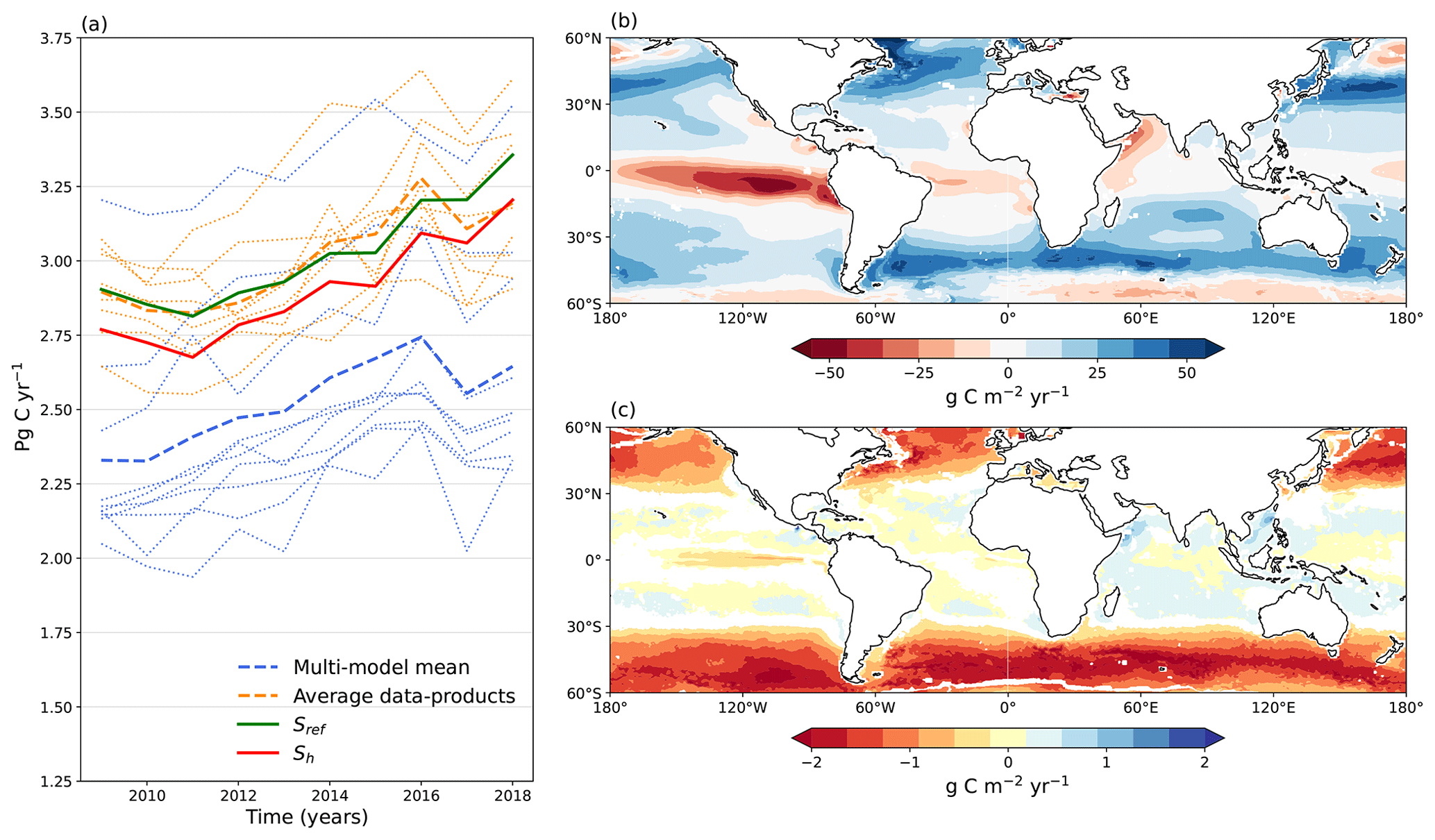
Figure 1 (a) Time series of the global (60° N–60° S) annual mean CO₂ sink (Pg C yr⁻¹) computed from S_ref (thick green line), S_h (thick red line), and the global annual mean from the GCB 2024 data products (thin orange lines) and their mean (thick dashed orange line) as well as the GCB 2024 models (thin blue lines) and their mean (thick dashed blue line). Also shown are maps for the 2009–2018 mean of (b) the air-sea CO₂ reference flux F_ref and (c) the difference between the monthly mean of the high frequency flux ${\stackrel{\mathrm{‾}}{F}}_{\mathrm{h}}$and F_ref, where positive values indicate less outgassing or more uptake with $\stackrel{\mathrm{‾}}{F_{\mathrm{h}}}$ than with F_ref.

3 Results

3.1 Global ocean carbon sink sensitivity to submonthly variability

Our estimate S_ref is comparable in magnitude to the average from the GCB data products although it does not capture the precise interannual evolution, in particular after 2016 (Fig. 1a). This difference stems from the latest version of the DIC and Alk OceanSODA-ETHZ dataset (v2021, Gregor and Gruber, 2021), which does not capture the change in Alk, DIC and fCO_2 sea associated with the slowdown in ocean sink after 2016 (e.g. Friedlingstein et al., 2022). This slowdown indeed only emerged in GCB data-based products after GCB 2023 (e.g. Friedlingstein et al., 2025). Both our S_ref and GCB account for submonthly variability of u. Our sink estimate S_h also accounts for submonthly variability of P_atm, T, and S, and it is 0.12 Pg C yr⁻¹ lower than S_ref. Therefore, the standard approach, which neglects all submonthly variability besides that of u, overestimates the carbon sink by 0.12 Pg C yr⁻¹. On average between 2009 and 2018, this difference corresponds to 5 % of the carbon sink S_ref but 25 % of the discrepancy between models and data products from GCB (∼ 0.5 Pg C yr⁻¹). Our computed difference does not change over 2009 to 2018 and remains statistically significant.

The spatial distribution of F_ref (Fig. 1b) is consistent with the fluxes from the SeaFlux product (Fay et al., 2021, Fig. S2). The 2009–2018 mean difference $\stackrel{\mathrm{‾}}{F_{\mathrm{h}}}-F_{\mathrm{ref}}$ shows that the discrepancy between the two fluxes stems largely from latitudes between 30 and 60° in both hemispheres (Fig. 1c). In these regions relative to F_ref, $\stackrel{\mathrm{‾}}{F_{\mathrm{h}}}$ exhibits either more outgassing (North Atlantic, Southern Ocean) or less uptake (North Pacific, by 1.5 g C m⁻² yr⁻¹ on average). A weaker opposing effect is seen in tropics, where sinks are increased by 0.5 g C m⁻² yr⁻¹ on average, and by up to 1 g C m⁻² yr⁻¹ in the Arabian Sea and South China Sea.

Differences in the mid-latitudes are mainly due to atmospheric pressure variations, whereas differences in the tropics are driven by sea surface temperature variations. The former can be seen in the $\stackrel{\mathrm{‾}}{F_P}-F_{\mathrm{ref}}$ map (Fig. 2a) and the $\stackrel{\mathrm{‾}}{F_{P,T}}-\stackrel{\mathrm{‾}}{F_P}$ map (Fig. 2b). Atmospheric pressure variations reduce the carbon sink estimate by 0.136 Pg C yr⁻¹ on average, an effect that is slightly weakened by sea surface temperature variations which increase the sink by 0.016 Pg C yr⁻¹. On synoptic timescales (2–10 d), low pressure perturbations are associated with stronger winds, so periods of strong CO₂ exchange have lower atmospheric pressure and thus lower atmospheric CO₂ fugacity. Thus wind speed and atmospheric pressure covariance leads to an anomalous outgassing correction term in the midlatitudes. Further separation of $\stackrel{\mathrm{‾}}{F_{P,T}}-\stackrel{\mathrm{‾}}{F_P}$ into atmospheric and oceanic components (Fig. S3b) reveal that temperature variations mainly affect ocean fCO_2 sea, but have negligible effect on vapor pressure. The anomalous ingassing in the Arabian Sea appears to result from an increase in submonthly variability of wind speed, which drives stronger upwelling and hence surface cooling, thus reducing fCO_2 sea. The remaining effect of salinity ($\stackrel{\mathrm{‾}}{F_{\mathrm{h}}}-\stackrel{\mathrm{‾}}{F_{P,T}}$) is negligible.

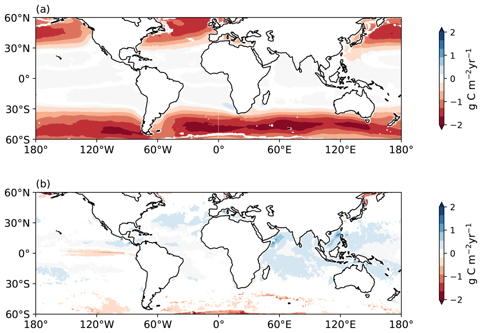
Figure 2 Maps averaged over 2009–2018 for effects on observation-based air-sea CO₂ fluxes from (a) submonthly variability of atmospheric pressure ($\stackrel{\mathrm{‾}}{F_P}-F_{\mathrm{ref}}$) and (b) submonthly variability of temperature ($\stackrel{\mathrm{‾}}{F_{P,T}}-\stackrel{\mathrm{‾}}{F_P}$).

3.2 Relative importance of the correction terms

The relative importance of the different terms is diagnosed by the Reynolds decomposition in Eq. (6). The wind speed variance term, which is already accounted for in the GCB data-based products, is the dominant source of submonthly nonlinearity (Fig. 3a). It results in an increase in the estimated 60° N–60° S ocean carbon sink by 0.36 Pg C yr⁻¹. This increase is situated mainly in the mid-latitudes, peaking at 40° S and 40° N (Figs. 3, S4).

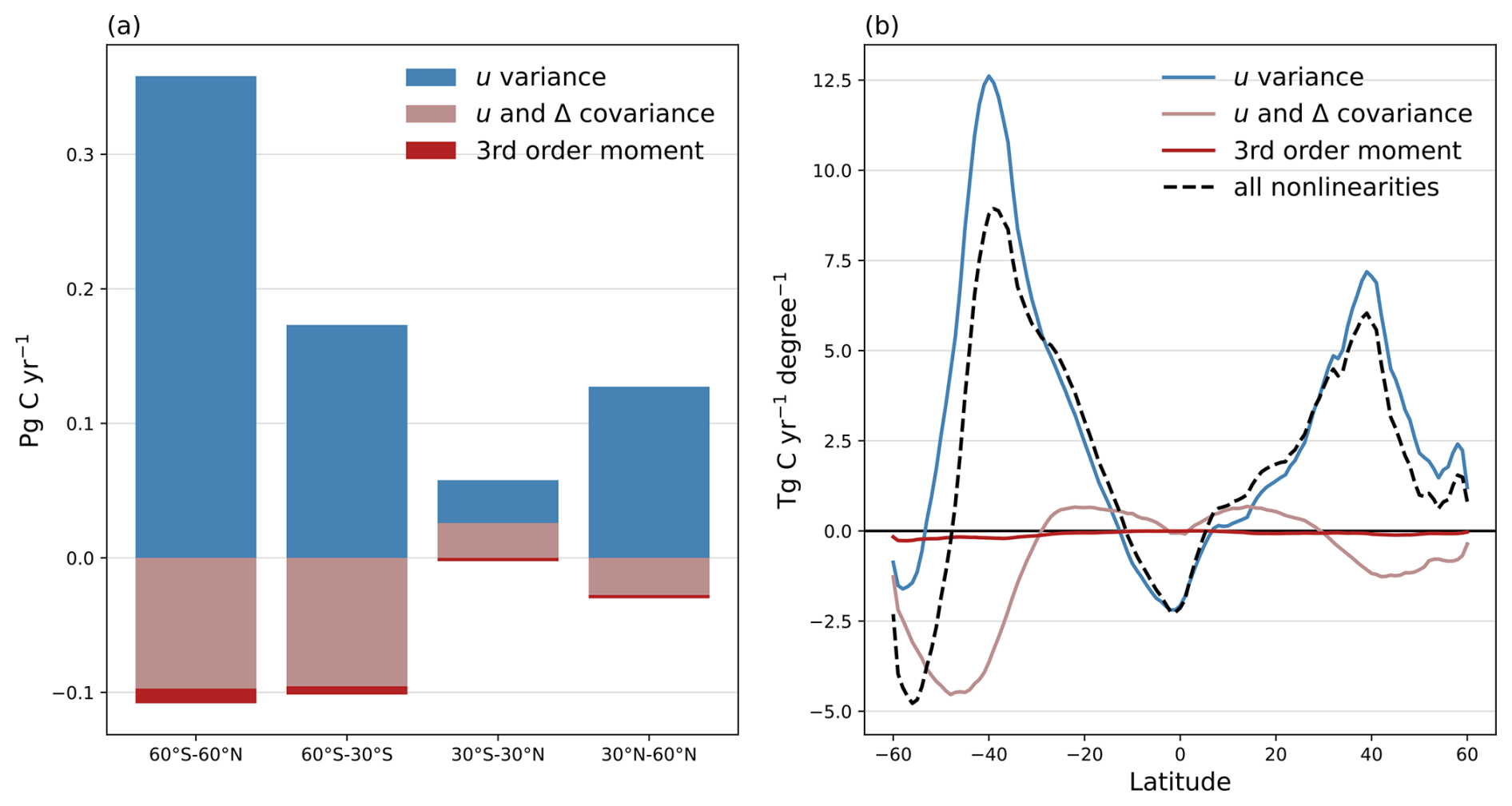
Figure 3 (a) Contribution of the final 3 terms in Eq. (6) to ocean carbon uptake in different latitudinal bands. (b) Zonal integral of the final three terms in Eq. (6) (blue, pink and red lines) and their sum (dashed black line).

Our first correction term (covariance) accounts for 90 % of the correction, whereas the third-order moment is weaker. Together they result in a global outgassing anomaly whose magnitude is one-third of the wind variance term and opposite in sign. About 85 % of this contribution is situated between 60–30° S and amounts to a reduction of 0.1 Pg C yr⁻¹ (Fig. 3a). The other main region where the correction terms reduce the sink is between 30–60° N, but that reduction of 0.03 Pg C yr⁻¹ is largely offset by the 0.026 Pg C yr⁻¹ increase between 30° S–30° N. Although the covariance term is generally weaker than the wind speed variance term, it has a similar magnitude in the tropics and dominates south of 50° S (Fig. 3b).

4 Discussion

This study reveals that accounting for hourly variability in atmospheric pressure and including the small compensation from daily variability in sea surface temperature, reduces data-based estimates of the global ocean carbon sink by 0.12 Pg C yr⁻¹, thereby closing 25 % of the gap between those data products and the GOBMs. While the 8 d product from Gregor et al. (2024) offers higher frequency atmospheric and oceanic CO₂ fugacities than the standard monthly products used in the GCB data-based ocean flux estimates, the resulting computed global flux is essentially unchanged. Thus, it appears that at least synoptic frequency is needed to adequately capture the effect of atmospheric variability. Whether or not 6-hourly or daily atmospheric pressure data would be sufficient in place of our use of hourly data remains a question for future research.

The Reynolds decomposition of the high-resolution CO₂ flux confirms that the submonthly variation in wind speed, already accounted for in the ocean data products, is the most important nonlinearity. It generally increases sink estimates outside the tropics with peaks at 40° S and 40° N. Conversely, our correction due to the submonthly covariance of wind speed and atmospheric pressure leads to outgassing anomalies in the midlatitudes. The reason is that midlatitude synoptic disturbances have strong winds that favor air-sea exchange but also reduce atmospheric pressure, thus lowering atmospheric CO₂ fugacity, which favors outgassing. This correction is particularly large in waters south of 30° S, representing 85 % of its impact on the global ocean carbon sink. South of 50° S, it becomes the main source of nonlinearity.

While the nonlinearities underlined here appear to explain 25 % of the average gap between models and data-based products, their effect seems constant in time. Therefore, they do not seem to explain the temporal evolution of the gap underlined by Friedlingstein et al. (2025). The exact correction will depend on the calculation details and thus will differ between data-based products. For future GCB exercises, we suggest that each group compute independently both directions of the flux k₆₆₀(u)A(T,S)fCO_2 atm and k₆₆₀(u)A(T,S)fCO_2 sea at maximum temporal resolution before computing monthly averages and taking the difference to obtain the flux. We also leave for future studies the question of whether or not accounting for submonthly variations in atmospheric $X_{{\mathrm{CO}}_{\mathrm{2}}}$, particularly those due to covariations with P_atm, may substantially alter data-based estimates of ocean carbon uptake. The gap between data-based products and GOBMs also depends on model resolution and their representation of coastal regions (e.g. Resplandy et al., 2024) as well as on processes not yet commonly included in the flux parameterization, such as the ocean cool skin (+0.3 Pg C yr⁻¹, Dong et al., 2022), rain (+0.14–0.19 Pg C yr⁻¹, Parc et al., 2024) and wave breaking-induced bubbles. While these bubbles may increase modeled CO₂ uptake by only 0.07 Pg C yr⁻¹ (Rustogi et al., 2025), they could increase data-based estimates by up to 0.3–0.4 Pg C yr⁻¹ (Dong et al., 2025). Similarly, Bellenger et al. (2023) showed that the cool skin temperature effect is three times smaller in a model framework because of the feedback process mentioned earlier and because gas exchange is not rate limiting, unlike carbon transfer to the ocean interior. Including the cool skin effect in both data-based products and GOBMs could thus increase the gap by about +0.2 Pg C yr⁻¹. The addition of new processes in the calculation of carbon fluxes may further increase the gap between estimates from data-based products versus GOBMs.

Our results suggest that the previous estimate of the storm-induced outgassing for the Southern Ocean of 0.057 Pg C yr⁻¹ (Carranza et al., 2024) is only a fraction of the total effect of submonthly variability on the ocean sink in this region. Indeed, we found a mean outgassing of about 0.1 Pg C yr⁻¹ in the 60–30° S band mainly driven by atmospheric pressure and wind speed covariance. On the other hand, previous observations in the Southern Ocean from Argo floats (Carranza et al., 2024) and gliders (Nicholson et al., 2022) suggest that submonthly variability of ocean biogeochemical variables have a major impact on storm induced outgassing. Those observations suggest that entrainment of cold, DIC-rich subsurface water into the surface mixed layer is the leading cause of mean storm-driven CO₂ outgassing in the Southern Ocean (Carranza et al., 2024). Monthly fCO₂-products cannot resolve storm induced fCO_2 sea, while GOBMs may underestimate storm-driven vertical transport of DIC (Carranza et al., 2024). Therefore, submonthly variability of biogeochemical variables in the Southern Ocean demands more attention, both for data- and model-based estimates. While our study helps to narrow the data-model gap, its continued growth and the large disparities among data-based products and among models underscore the need for further advances to constrain ocean carbon uptake, advances that are also key to reducing, by difference, much larger uncertainties associated with the terrestrial biosphere.