Resolving distribution and controls of terrigenous and marine particulate organic matter across an energetic shelf

We assess the sources, distribution and controls of particulate organic matter (POM) across the northeastern Taiwan Strait, where monsoonal forcing, water-mass mixing, riverine inputs and sediment resuspension modulate particle dynamics. By integrating lignin biomarkers, bulk geochemistry, and sedimentary constraints within a two-step quantification approach, we demonstrate the influence of river discharge, plume intrusions, and seafloor resuspension on the distribution of terrigenous POM. Terrigenous particulate organic carbon (POC_terr) represents a minor component in most water samples but becomes substantial in resuspension-dominated layers. Combining estimated POC_terr with modeled current velocities yields an export flux of ∼ 243±56 kt C yr⁻¹, consistent with the regional imbalance between riverine input and sedimentary burial. After correction for terrigenous influence, bulk POM parameters reflect nutrient supply, photoacclimation, and temperature-dependent variation in stable carbon isotopic (δ¹³C) composition. Comparisons with co-sampled surface sediments show that biomarker signals are preserved more faithfully than δ¹³C of organic matter, which is strongly modulated by lateral transport. This study provides a practical framework for quantifying terrigenous and marine POM in continental-shelf settings and offers improved constraints for interpreting source-to-sink processes and sedimentary archives.

1 Introduction

Continental shelves are widely recognized as critical interfaces in the global carbon cycle, although they represent only 5 % of the ocean area (Dunne et al., 2007). These environments receive substantial inputs of terrigenous and marine organic matter (OM) and are estimated to account for up to 85 % of global organic carbon (OC) burial (Burdige, 2005, 2007). To constrain the fate and long-term sequestration efficiency of OM in individual shelf systems, quantitative characterization of marine and terrigenous OM sources is essential. Extensive research has focused on characterizing the sources of OM in shelf sediments (e.g., Bao et al., 2018; Tao et al., 2023; Wei et al., 2020), yet the provenance of particulate organic matter (POM) suspended in the water column remains insufficiently resolved. This knowledge gap limits our understanding of modern source-to-sink processes and undermines confidence in paleoenvironmental reconstructions based on sedimentary OM.

Bulk geochemical parameters of OM, such as atomic C $/$ N ratio, the mass ratio of OC to chlorophyll a (OC $/$ Chl), and the stable carbon isotopic ratio of OC (δ¹³C_OC), have been widely used to constrain POM sources (e.g., Gao et al., 2014; Guo et al., 2015; Lee et al., 2023). However, their capacity to distinguish complex POM mixtures in shelf waters is limited. Shelf waters receive terrigenous POM inputs from rivers and from sediment resuspension, and these two sources may differ in bulk properties depending on the extent of OM partitioning during transport and resuspension (Lin et al., 2025a). In addition, marine plankton communities, particularly primary producers, can produce bulk POM signatures that overlap with those of terrigenous OM (e.g., Geider, 1987; Laws et al., 1995; Martiny et al., 2013). This ambiguity is illustrated by the frequent observation of ¹³C-depleted POM in subsurface and bottom shelf waters (e.g., Wu et al., 2003; Huang et al., 2020a; Lee et al., 2023). In contrast to open-ocean settings, where a terrigenous source for the low-δ¹³C POM in the lower euphotic zone can generally be excluded (Close and Henderson, 2020), the proximity of shelf waters to land makes it difficult to determine whether such isotopic signals primarily reflect terrigenous inputs or in situ marine processes. To alleviate these complications, previous studies have focused on sampling layers where a single POM source is expected to dominate, such as the deep Chl maximum (DCM) or the benthic nepheloid layer (e.g., Liu et al., 2018a; Sun et al., 2024). Although informative for process-oriented investigations, these strategies do not provide an integrated view of POM mixing and transport throughout the water column.

Two complementary approaches may help address this limitation. The first involves the use of biomarkers that provide diagnostic information on specific OM sources. Lignin is an abundant and stable biopolymer found exclusively in the cell walls of vascular plants (Benner et al., 1987; Hedges et al., 1997). Because vascular plants are largely restricted to land, lignin serves as unambiguous tracers for terrigenous OM. Lignin has been widely applied to trace terrigenous inputs in marine sediments (e.g., Bianchi et al., 2018), but its use in POM studies remains limited. The second approach involves characterizing surface sediments collected concurrently with POM to constrain the contribution from resuspension. This strategy was implemented by Sun et al. (2024), who quantitatively evaluated how sediment reworking influences the distribution and degradation of terrigenous POM. Together, these constraints offer a way to better distinguish terrigenous contributions to POM and to clarify how bulk geochemical parameters relate to the condition of marine plankton communities.

The overarching goal of this study is to provide a full-water-column assessment of the sources, distribution, and controls of POM in the northeastern Taiwan Strait, a shallow and energetic shelf system (Fig. 1). The properties and spatial distribution of OM in surface sediments collected concurrently with the POM samples were presented in our earlier study (Lin et al., 2025a). The present work builds on this foundation through three objectives. First, we quantify terrigenous particulate organic carbon (POC_terr), defined as the sum of biospheric and petrogenic OC, using lignin and δ¹³C_OC as key tracers within an integrated two-step quantitative approach. The inclusion of lignin provides an additional constraint for identifying the sources of low-δ¹³C POM, which is also observed in our study area. Second, we examine the biogeochemical characteristics of the remaining marine POM and evaluate the associated physiological controls. Finally, we establish source-to-sink coherence by comparing POM characteristics in the water column, which reflect short-term transport processes, with the OM composition recorded in surface sediments. This comparison provides insights into OM transport dynamics and supports more robust interpretations of OM proxies in shelf sediment archives.

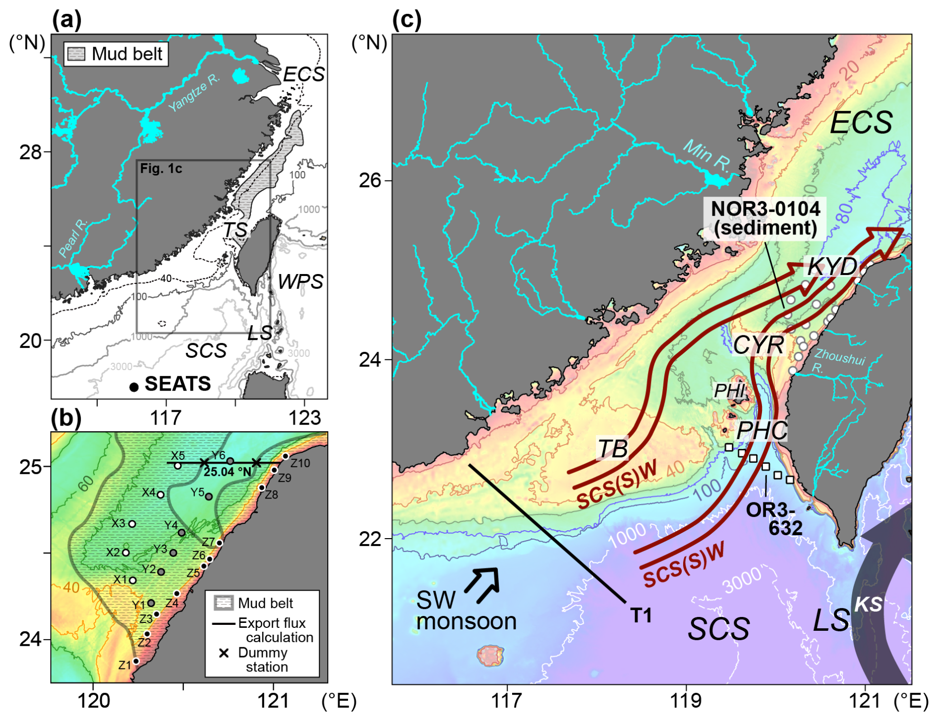
Figure 1 Study area and sampling sites. (a) Study area relative to China and Taiwan. The SEATS station (Liu et al., 2007) is also shown. ECS, East China Sea; LS, Luzon Strait; SCS, South China Sea; TS, Taiwan Strait; WPS, West Philippine Sea. (b) Seawater sampling sites from the cruise NOR3-0104. The extent of mud belts (mean grain size <63 µm) was based on the isosurface map of sediment grain size (Lin et al., 2025a). (c) Bathymetry and summer flow field (redrawn from Jan et al., 2010). Also shown are seabed sediment sampling sites from cruise NOR3-0104 (Lin et al., 2025a), legacy stations from cruise OR3-632 (Ocean Data Bank, 2025), and Transect T1 from Wong et al. (2015). Bathymetric features: Changyun Rise (CYR), Kuanyin Depression (KYD), Penghu Channel (PHC), Penghu Islands (PHI), and Taiwan Bank (TB). Currents or water masses: KS, Kuroshio; SCS(S)W, South China Sea (Surface) Water.

2 Material and Methods

2.1 Study area

The Taiwan Strait is a shallow and energetic conduit linking the South China Sea and East China Sea (Fig. 1). Bounded by the Chinese coast to the west and the island of Taiwan to the east, the strait averages ∼ 60 m in depth, extends ∼ 350 km in length, and spans ∼ 180 km in width (Jan et al., 2002). Its hydrography is highly dynamic, shaped by the interplay of complex bathymetry, monsoonal forcing, and riverine inputs.

Because sampling was conducted in summer, the following description emphasizes the hydrographic conditions of this season. During summer, under the influence of the southwest monsoon, the Taiwan Strait exhibits a net northeastward transport (Jan et al., 2002). Oceanic waters from the northern South China Sea enter the strait either along the shelf off southeastern China or through the funnel-shaped Penghu Channel, which serves as the primary pathway for volume transport during this season (∼ 1.2 × 10⁶ m³ s⁻¹; Jan et al., 2002). The inflow is dominated by the South China Sea Water (SCSW), reflecting the limited intrusion of the Kuroshio into the northern South China Sea through the Luzon Strait during summer (Jan et al., 2006, 2010). The upper water column, typically above 40 m, is characterized by the South China Sea Surface Water (SCSSW), a brackish water mass influenced by Pearl River discharge (Bai et al., 2015; Jan et al., 2006). In the northeastern Taiwan Strait, which is the focus of this study, additional freshwater inputs are supplied by small rivers from Taiwan. Tidal dynamics are dominated by the semidiurnal M2 constituent, which has a period of 12.42 h and produces strong oscillatory currents particularly in the Penghu Channel and Kuanyin Depression. Tidal current amplitudes decreased from ∼ 0.8 m s⁻¹ at the northeast and southeast entrances to ∼ 0.2 m s⁻¹ in the central strait (Wang et al., 2003).

The modern sedimentary regime of the Taiwan Strait has been documented previously (Huh et al., 2011; Liu et al., 2018b). The region receives substantial sediment from both the distal Yangtze River and the proximal small mountainous rivers of Taiwan, supporting a mud-rich deposition system that extends for more than 1000 km. In the northeastern Taiwan Strait, sedimentation is organized into two mud belts that are primarily sourced from Taiwan (Horng and Huh, 2011; Lin et al., 2025a). The Taiwan Along-Shore Mud Belt, referred to here as the nearshore mud belt, forms as fine sediments are deposited near river mouths and subsequently transported northward through resuspension-advection processes. This belt is enriched in fresh terrigenous OM, largely derived from vascular plants. Further offshore, the Cross-Shelf Mud Belt, referred to here as the offshore mud belt, spatially overlaps with a depocenter characterized by high sedimentation rates and contains terrigenous OM predominantly of petrogenic origin. These characteristics suggest that this mud belt is formed through hyperpycnal or other gravity-driven transport processes triggered by typhoons and floods.

Primary production, determined across the Changyun Rise, exhibits pronounced seasonality, with summer productivity reaching 664±270 mg C m⁻² d⁻¹ (Tseng et al., 2020). The summer maximum corresponds to enhanced offshore Chl concentrations integrated over the euphotic zone. The elevated offshore production during summer has been attributed to nutrient supply transported from upwelling zones near the Taiwan Bank and the Penghu Islands.

2.2 Fieldwork

A total of 21 sites in the northeastern Taiwan Strait were surveyed aboard the RV New Ocean Researcher 3 during cruise NOR3-0104 (13–21 June 2022) (Table A1 in Appendix A). These sites were arranged along three SW–NE transects (X, Y, and Z), spanning the nearshore and offshore mud belts (Fig. 1b). At each station, we deployed a conductivity-temperature-depth (CTD) rosette system (SBE911plus, Sea-Bird Scientific) equipped with 12 L Niskin bottles for simultaneous acquisition of hydrographic data and water samples. Dissolved oxygen, fluorescence, beam attenuation, and photosynthetically active radiation were monitored using onboard sensors (SBE43 and C-Star, Sea-Bird Scientific; Aqua Tracka III and PAR sensor, Chelsea Instruments Ltd.). Surface water samples from the air-sea interface were collected using a clean bucket, and their temperature and salinity were immediately measured with a portable conductivity meter (Cond 3110, WTW).

Each water sample was divided into three or four aliquots for different purposes. For bulk and Chl analyses, 1–2 L of water was filtered through pre-combusted glass fiber filters (GF75, Advantec; diameter: 25 mm, pore size: 0.3 µm). For lignin analysis, 3–4 L of water was filtered using the same filter type but with a larger diameter (47 mm). All filters were stored in the dark at −20 °C until analysis. Additional aliquots for carbonate chemistry (n= 28; Table A1) were collected following Huang et al. (2012, 2020b). These samples were transferred into 250 mL borosilicate glass bottles fitted with a drip-free polypropylene pouring ring, poisoned with 60 µL of saturated HgCl₂ solution, sealed with a screw cap, and stored in the dark at room temperature.

2.3 Analytical procedures

Total suspended matter (TSM) concentrations were determined gravimetrically. Filters were first examined under a microscope to remove visible zooplankton and plastic debris. Decalcified filters were analyzed for particulate organic carbon (POC), particulate organic nitrogen (PON), and δ¹³C_OC using an elemental analyzer coupled to an isotope ratio mass spectrometer (Flash 2000 and Delta V Plus; Thermo Fisher Scientific), following procedures detailed in Lin et al. (2020a). The relative analytical error was 3 % for POC and PON, yielding a 4 % relative uncertainty for calculated atomic C $/$ N or N $/$ C ratios. The absolute error for δ¹³C_OC was 0.4 ‰.

For Chl analysis, filter samples were extracted in cold acetone within one month after collection, and Chl concentrations were quantified fluorometrically (10-AU; Turner Designs, Inc.) following Aminot and Rey (2001).

Lignin phenols, recognized biomarkers diagnostic of vascular plant inputs, were extracted using cupric oxide oxidation (Hedges and Ertel, 1982). Filters and reagents were placed into a polytetrafluoroethylene liner, to which 8 mL of argon-purged 2 N NaOH was added. After purging the headspace with argon, the liner was sealed in a stainless-steel vessel and heated at 170 °C for 3 h. The resulting hydrolysate was acidified with HCl and spiked with the internal standard ethyl vanillin, and the target compounds were extracted into ethyl acetate via liquid-liquid extraction. The extracts, condensed passively at 40 °C, were derivatized using a 1:1 mixture of N,O-bis(trimethylsilyl)trifluoroacetamide and pyridine to a final volume of 10 µL, and analyzed by gas chromatography-mass spectrometry (7890A and 5957C; Agilent Technologies, Inc.) using an HP-5MS capillary column (30 m × 0.25 mm, film thickness 0.25 µm; Technologies, Inc.). Method detection limits, calculated as 3.14 times the standard deviation of replicate low-concentration standards (n= 6) following U.S. EPA guidelines, were about 15 ng L⁻¹ for the sum of eight lignin monomers. Replicate analysis of a sediment standard indicated 5 %–20 % variability among individual phenols. We report the sum of eight lignin monomers per unit volume of water (Σ8), OC normalized concentration (Λ8), and the mass ratio of vanillic acid to vanillin ((Ad $/$ Al)_V) (Hedges and Ertel, 1982). A higher (Ad $/$ Al)_V ratio indicates more extensive lignin degradation.

Dissolved inorganic carbon (DIC) was measured using a DIC analyzer (AS-C3, Apollo SciTech, LLC). Samples were acidified with 10 % phosphoric acid, and the released CO₂ was quantified via a CO₂ analyzer (LI-7000, LI-COR, Inc.). Analytical quality was ensured using certified reference materials from Andrew Dickson at the Scripps Institute of Oceanography, yielding precision and accuracy better than 0.1 % (Huang et al., 2012). pH measurements were performed spectrophotometrically (Varian Cary-50, Agilent Technologies, Inc.) in a 10 cm quartz cell at 25±0.5 °C (pH₂₅), following Clayton and Byrne (1993). Measurement precision, assessed using unpurified m-cresol purple, was < 0.003.

3 Data

3.1 Data sources and previously published data

A subset of the hydrographic observations used in this study was previously reported in Lin et al. (2025a), which focused primarily on sediment geochemistry. In that study, Chl, surface-water salinity, bottom-water temperature, and bottom-water TSM were used only to provide environmental context. Lin et al. (2025b), archived in Zenodo, is the companion dataset for the present study and provides the underlying measurements, including POM geochemical data analyzed and discussed here for the first time.

3.2 Processing of hydrographic data

A total of 64 samples were analyzed to calibrate sensor measurements of beam attenuation (Atten) and fluorescence (FL). The resulting calibration equations are:

$$\begin{array}{}\text{(1)}& {\displaystyle }\mathrm{TSM}=\mathrm{2.6427}\times \mathrm{Atten}+\mathrm{0.8053},r^{\mathrm{2}}=\mathrm{0.90}\text{(2)}& {\displaystyle }\mathrm{Chl}=\mathrm{0.7176}\times \mathrm{FL}+\mathrm{0.2523},r^{\mathrm{2}}=\mathrm{0.74}\end{array}$$

where TSM is in mg L⁻¹, Atten in m⁻¹, Chl in µg L⁻¹, and FL in µg L⁻¹.

The euphotic depth (Z_e) was defined as the depth of 1 % surface light penetration. Photosynthetically active radiation measurements were available only for 11 daytime stations (Table A1). For the remaining sites, Z_e was estimated from bottom water depth (Z_bot) using the linear relationship derived from these 11 stations:

$$\begin{array}{}\text{(3)}& Z_{\mathrm{e}}=\mathrm{0.5402}\times Z_{\mathrm{bot}}+\mathrm{3.0745},r^{\mathrm{2}}=\mathrm{0.83}\end{array}$$

where both Z_e and Z_bot are in meters.

To provide regional hydrographic context for our observations, the following summer temperature–salinity (T–S) datasets were incorporated into the analysis. The first consists of typical SCSW and Kuroshio Water compiled by Jan et al. (2010). The second comprises observations from Transect T1, which extends from the continental shelf west of the Taiwan Bank to the open South China Sea (Fig. 1c; Wong et al., 2015).

3.3 Processing of geochemical data

3.3.1 Estimation of POC_terr

We developed a two-step approach to quantify POC_terr (details in Sect. B1 and B2 of Appendix B). Figure 2 summarizes the workflow. This approach combines the complementary strengths of lignin biomarkers and δ¹³C in diagnosing and quantifying terrigenous OM in the water column.

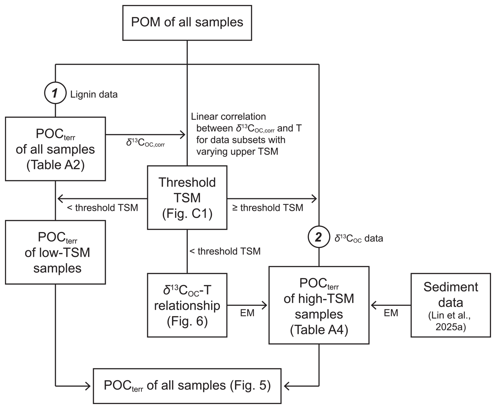
Figure 2 Schematic diagram summarizing the data processing procedure for estimating POC_terr. EM, endmember; T, temperature.

In the first step, lignin concentrations were used primarily to assess the relative abundance of terrigenous OM, particularly in low-δ¹³C samples where source attribution based on isotopic composition alone may be ambiguous. Elevated Λ8 values were expected if low-δ¹³C POM contained a greater terrigenous contribution. The spatial patterns of lignin and its correlation with environmental variables indicated three potential sources (see Sect. 4.3; Table A2): (i) Pearl River TSM for offshore surface waters, (ii) Taiwanese river TSM for nearshore waters, and (iii) seabed sediments for benthic nepheloid layers.

Following source identification, POC_terr was estimated from lignin concentrations assuming characteristic lignin-to-POC_terr ratios (Λ8_terr) in the source material:

$$\begin{array}{}\text{(4)}& {\mathrm{POC}}_{\mathrm{terr}}=\mathrm{\Sigma }{\mathrm{8}}_{\mathrm{m}}/\mathrm{\Lambda }{\mathrm{8}}_{\mathrm{terr},\mathrm{s}}\end{array}$$

where the subscript m denotes measured POM data and s the inferred source. Source-specific Λ8_terr,s values were taken from Zhang et al. (2014) and Lin et al. (2025a) (Table A3). Mixing equations were then applied to derive POC, N $/$ C, and δ¹³C_OC values corrected for terrigenous inputs (POC_corr, N $/$ C_corr, δ¹³C_OC,corr).

However, lignin-based estimates of POC_terr are subject to uncertainty because Λ8_terr,s can vary during particle transport (Wakeham et al., 2009). This limitation motivated the second step, in which a δ¹³C-based mixing model was applied to samples with high TSM. Based on their spatial distribution, these samples can be reasonably attributed to resuspended seabed sediment (cf. Sect. 4.3), allowing more reliable assignment of endmember δ¹³C values. To define high-TSM samples operationally, we ranked the dataset by TSM and evaluated the correlation between δ¹³C_OC,corr (from Step 1) and temperature (cf. Sect. 5.2.3) for subsets with progressively increasing upper TSM limits. The correlation deteriorated when samples with samples with TSM ≥ 4 mg L⁻¹ were included (Fig. C1 in Appendix C). Therefore, this value was adopted as the threshold separating low- and-high TSM samples.

The δ¹³C-based binary mixing model treats POC as a mixture of sedimentary and marine OC. Sedimentary endmembers were site-specific, whereas marine endmembers were derived from the δ¹³C_OC-temperature relationship of low-TSM samples (cf. Sect. 5.2.3). POC_terr was calculated as:

$$\begin{array}{}\text{(5)}& {\mathrm{POC}}_{\mathrm{terr}}={\mathrm{POC}}_{\mathrm{m}}\times f_{\mathrm{sed}}\times f_{\mathrm{terr},\mathrm{sed}}\end{array}$$

where POC_m is measured POC, f_sed the sedimentary fraction of POC derived from the binary mixing model, and f_terr,sed the terrigenous fraction of sedimentary OC (Table A4). In this step, δ¹³C_OC,corr could not be obtained because δ¹³C_OC was prescribed from the δ¹³C_OC-temperature relationship. Therefore, only POC_corr and N $/$ C_corr were computed for high-TSM samples. The estimated f_sed values were further used to calculate the source signature of Λ8 (Λ8_cal) required to account for the measured Λ8 (Λ8_m) in high-TSM samples:

$$\begin{array}{}\text{(6)}& \mathrm{\Lambda }{\mathrm{8}}_{\mathrm{cal}}=\mathrm{\Lambda }{\mathrm{8}}_{\mathrm{m}}/\left(f_{\mathrm{sed}}\times f_{\mathrm{terr},\mathrm{sed}}\right)\end{array}$$

Comparison of Λ8_m and the corresponding Λ8_terr,s used in Step 1 helps evaluate the limitations and uncertainties of lignin-based POC_terr quantification.

3.3.2 Estimation of POC_terr export flux

To compare with the riverine flux from Taiwan, the advective export flux of POC_terr was estimated by combining POC_terr concentrations with flow data from the Hybrid Coordinate Ocean Model (HYCOM). The applicability of HYCOM for reconstructing water flux through the strait has been validated by Huang et al. (2019). A latitudinal transect between 120.40 and 121.04° E at 25.04° N was defined as the northern boundary of the study area (Fig. 1b), and export flux was calculated as the rate of material crossing this transect.

POC_terr estimates from Step 1 were used for low-TSM samples and those from Step 2 for high-TSM samples. POC_terr in offshore surface waters, attributable to remote Pearl River inputs (see Sect. 5.1.1), was excluded. The bottommost 5 m of the water column was also omitted due to (i) the lack of CTD data, and (ii) the higher likelihood of particle re-deposition near the seafloor. Calculation details are provided in Sect. B3.

3.3.3 Calculation of dissolved CO₂ concentration

For samples with carbonate chemistry measurements, we used CO2SYS Version 3 (Pierrot et al., 2021) to compute dissolved CO₂ (CO₂(aq)) concentrations from measured DIC and pH₂₅ (Table A5). Due to the lack of concurrent nutrient data, we incorporated historical records from Sites A to F, which were visited during the cruise OR3-632 of RV Ocean Researcher III in June 2000 (Fig. 1c). These sites exhibit similar water mass characteristics to those in our study area (Fig. C2). These data were accessed from the Ocean Data Bank (2025). Salinity-based empirical relationships for silica and phosphate were derived from these records (Fig. C3) and then applied to provide the nutrient inputs required for CO2SYS calculations for NOR3-0104 samples.

3.4 Statistical analysis and visualization

Statistical analyses were conducted using Excel^® add-ons XLSTAT (Lumivero). The non-parametric Mann-Whitney test was used for comparing two datasets, and the Kruskal-Wallis test followed by Dunn's test was used for comparisons among three datasets. Differences between slopes of two linear regressions were tested using Student's t-test following Andrade and Estévez-Pérez (2014). Statistical significance was set at α= 0.05. Bathymetric maps and topographic profiles were generated in QGIS (version 3.34.11) using digital elevation models from the Ocean Data Bank (2025) referenced to WGS 84. Transects with isopleths were created using Ocean Data View (version 5.6.3; Schlitzer, 2025).

4 Results

4.1 Hydrographic data

Hydrographic data are available in Lin et al. (2025b), and their vertical distributions are shown in Fig. 3. Temperature ranged from 23.4 to 30.0 °C (Fig. 3a), highest along the Taiwanese coast and lowest in the bottom water at Site X5. Salinity showed the opposite pattern, increasing from 32.8 nearshore to 34.3 offshore (Fig. 3b). In the T–S diagram (Fig. C2), most samples clustered near the typical SCSW curve, while two subsets exhibited lower salinity. One subset, with higher potential density (σ_θ) values (21.7–22.5 kg m⁻³), comprised upper-water-column samples from Transects X and Y and overlapped with middle-shelf waters in Transect T1. This subset is therefore attributed to the SCSSW. The other subset, having lower σ_θ values (< 21.7 kg m⁻³), occupied nearly the entire water column in Transect Z. Given its proximity to the Taiwanese coast, this subset is hereafter referred to as Taiwan Coastal Water (TCW).

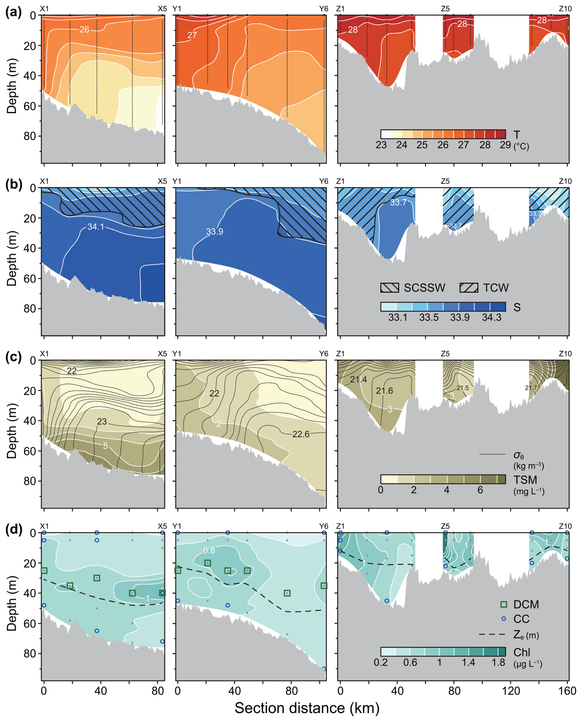
Figure 3 Hydrographic conditions along three transects in the northeastern Taiwan Strait during summer 2022. (a) Temperature, with black dots marking CTD measurement points. (b) Salinity and distribution of South China Sea Surface Water (SCSSW) and Taiwan Coastal Water (TCW). (c) TSM and σ_θ. (d) Chl concentrations and Z_e. Grey dots indicate depths for discrete water sampling.

After calibration (Eq. 1), sensor-derived TSM ranged from 0.7 to 36.4 mg L⁻¹ (Fig. 3c). High TSM occurred in bottom waters (> 40 m) of Sites X1–X5 and Y1–Y4, and throughout Transect Z. At weakly stratified sites (X1, Y1, and Z10), bottom-enriched TSM reached the surface.

Calibrated Chl (Eq. 2) ranged from 0.2 to 2.5 µg L⁻¹ (Fig. 3d). Chl-rich waters (exceeding ∼ 1 µg L⁻¹) occurred at 10–40 m depths in Transects X and Y and throughout Transect Z, particularly near river mouths (Z1, Z2, Z5, Z8, and Z9).

4.2 POM data

POM data are available in Lin et al. (2025b) and displayed in Fig. 4. POC ranged from 63 to 578 µg L⁻¹ (Fig. 4a), higher in nearshore than offshore waters. Surface POC (0–5 m) exceeded subsurface values (p= 0.006). Elevated bottom-water POC at Sites X1–X3, Z9, and Z10 coincided with high TSM concentrations (Fig. 3c).

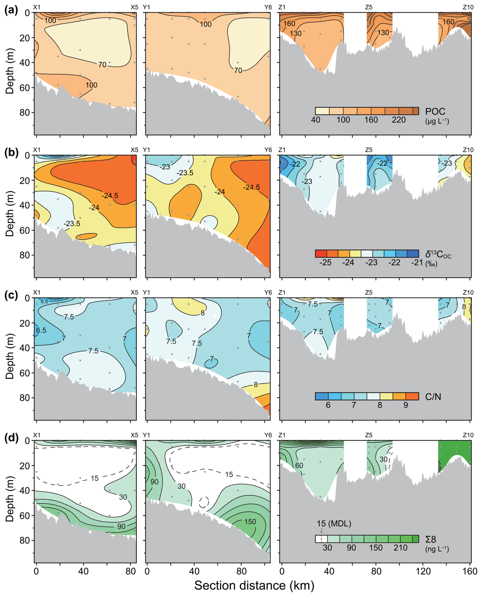
Figure 4 POM characteristics along the three transects in the northeastern Taiwan Strait during summer 2022. (a) POC concentrations. (b) δ¹³C_OC values. (c) Atomic C $/$ N ratios. (d) Σ8 concentrations. Grey dots indicate depths for discrete water sampling. MDL, method detection limit.

δ¹³C_OC values ranged from −25.1 ‰ to −21.0 ‰, with heavier values nearshore than offshore (Fig. 4b). Most high-POC samples, except turbid samples at Sites Z9 and Z10, had δ¹³C_OC values above −23 ‰. Low-δ¹³C (<−24 ‰) POM occurred in subsurface and bottom waters of Transects X and Y. C $/$ N ratios (6.4–10.0) lacked clear spatial or vertical patterns (Fig. 4c). C $/$ N ratios >8 occurred in surface waters of Y1–Y3 and Z2–Z4, in bottom waters of Y6, and throughout Z10.

Σ8 ranged from below detection to 2,753 ng L⁻¹ (Fig. 4d). Where measurable, Λ8 ranged from 0.12 to 8.6 mg lignin g⁻¹ OC. In offshore Transects X and Y, Σ8 were elevated in surface and bottom waters but remained below detection in subsurface waters. Λ8 showed no significant difference between samples with δ¹³C_OC values below and above −24 ‰ (p= 0.489). Transect Z exhibited higher Σ8 than the offshore transects (p≤ 0.001), particularly at high-TSM sites (Z1–Z2, Z5, Z8–Z10). Most (Ad $/$ Al)_V values ranged from 0.1 to 2; four anomalously high values (2.5–5) likely resulted from incomplete oxygen sparging during sample pretreatment. After excluding these samples, Transect Z ((Ad $/$ Al${)}_V=\mathrm{0.54}\pm \mathrm{0.28}$) had lower degradation state than the other transects (mean = 1.10; p≤ 0.004).

4.3 Estimated POC_terr concentrations

Applying Eq. (4) requires defining terrigenous POM sources (Tables A2 and A3). Σ8 correlated strongly with TSM (r= 0.79, p<0.0001) and moderately with salinity ($r=-\mathrm{0.42}$, p<0.0001) (Figs. 5a–b), indicating sediment resuspension as the dominant lignin source. Muddy sediments, richer in lignin than sand (Lin et al., 2025a; Fig. C4), likely supplied most lignin. Enrichment of lignin also occurred in surface waters. Surface lignin in Transect Z likely originated from Taiwanese rivers, whereas that in Transects X and Y is attributed to long-distance transport from the Pearl River, consistent with summer circulation (Fig. 1c).

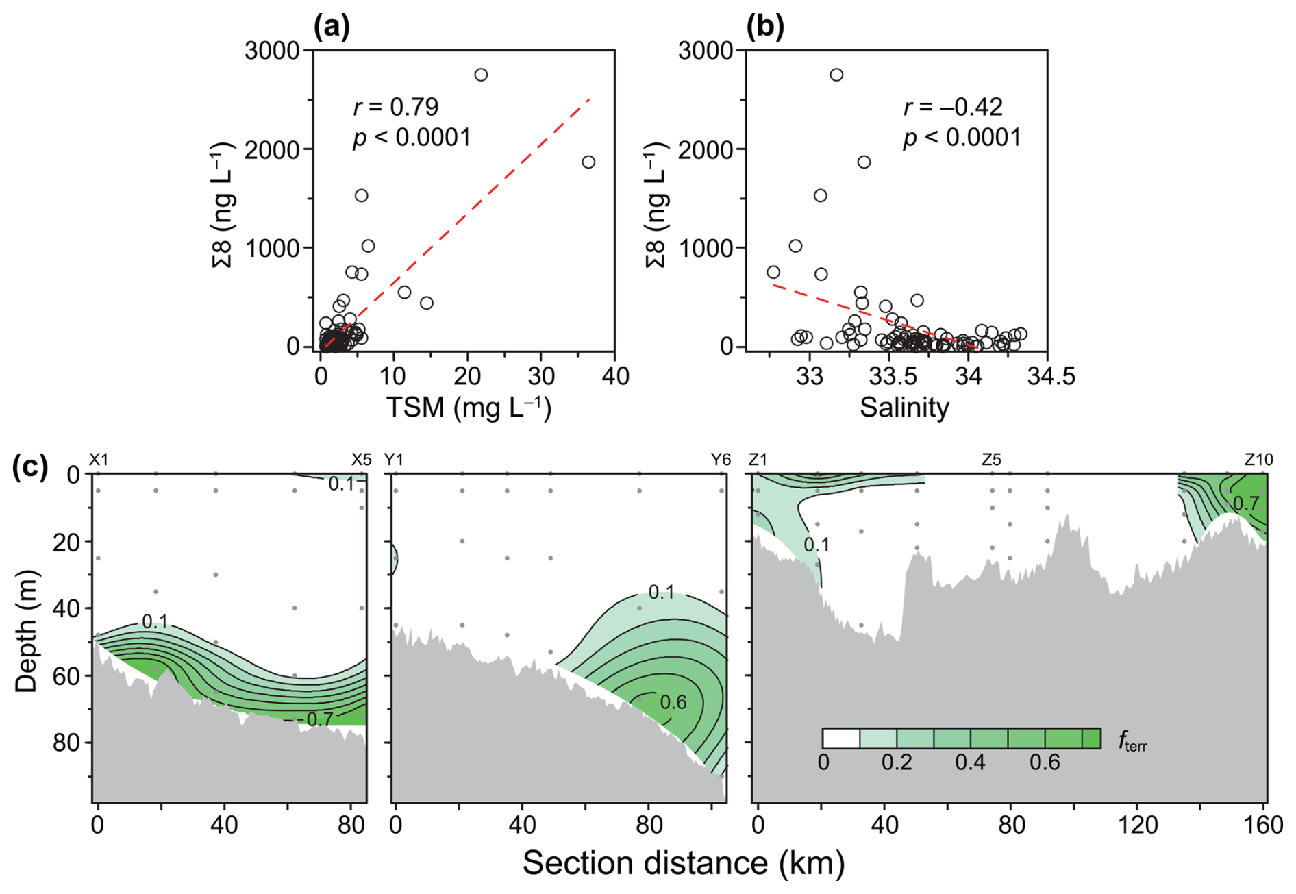
Figure 5 Characteristics of terrigenous POM. (a) Relationship between Σ8 and TSM. (b) Relationship between Σ8 and salinity. (c) Spatial distribution of f_terr along the three transects in the northeastern Taiwan Strait during summer 2022. Grey dots indicate depths for discrete water sampling.

Lignin-based POC_terr values and corrected POM parameters (POC_corr, N $/$ C_corr, and δ¹³C_OC,corr) after Step 1 are listed in Table A2. POC_terr concentrations did not exceed 63 µg L⁻¹ and were below 10 µg L⁻¹ for most samples. The terrigenous fraction of POC (f_terr), calculated as POC_terr/POC_m, averaged 0.06±0.07 for all samples. Relative differences between measured and corrected values averaged 6.4 % for POC and < 1 % for C $/$ N and δ¹³C_OC.

The δ¹³C_OC-based mixing model of the second step yielded POC_terr= 47–332 µg L⁻¹ and f_terr= 0.47–0.92 for high-TSM samples (Table A4). For comparison, lignin-based f_terr values were 0.03–0.69 for the same set of samples. Λ8_cal averaged only 17±10 % of Λ8_terr,s (Table A4). Combined results (Steps 1 and 2) show f_terr > 0.5 in offshore bottom waters along Transect X, at Site Y5, and in nearshore waters at Z9–Z10 (Fig. 5c).

4.4 Estimated POC_terr export flux

POC_terr concentrations derived from the combined approach, i.e. lignin-based estimates for low-TSM samples and δ¹³C-based estimates for high-TSM samples, were used to calculate the POC_terr export flux. Along 25.04° N, POC_terr concentrations were elevated in nearshore and offshore bottom waters (Fig. C5a). The annually averaged flow was northeastward, but highest velocities occurred where POC_terr was low (Fig. C5b). Thus, POC_terr export was controlled mainly by concentration rather than current speed (Fig. C5c). The total export flux was 243±56 kt C yr⁻¹.

4.5 Carbonate chemistry

Carbonate chemistry data are available in Lin et al. (2025b). DIC ranged from 1807 to 2007 µmol kg⁻¹, lowest at 0 m of Site X3 and highest at 72 m of Site X5. pH₂₅ ranged from 7.96 (72 m of Site X5) to 8.13 (0 m of Site Z5). Computed CO₂(aq) concentrations ranged from 8.7 to 13.9 µmol kg⁻¹ (equivalent to 8.9 to 14.2 µmol L⁻¹), with minimum and maximum values occurring at Sites Z5 and X5, respectively (Table A6).

5 Discussion

5.1 Distribution and budget of terrigenous POM

5.1.1 Persistence of lignin and POC_terr at low abundance during advective transport

The fate of terrigenous OM in the ocean has long intrigued geochemists (Bianchi, 2011; Hedges et al., 1997; Talling et al., 2024). Globally, rivers deliver ∼ 200 Mt yr⁻¹ of POC to the ocean, ∼ 80 % biospheric and ∼ 20 % petrogenic (Galy et al., 2015), yet only 62–90 Mt yr⁻¹ is ultimately buried (Talling et al., 2024). One explanation for this imbalance is repeated settling-resuspension cycles in estuarine and coastal waters, which weaken organo-mineral associations and enhance OM bioavailability (Bao et al., 2018; Burdige, 2007; Sun et al., 2024). What remains uncertain is whether the terrigenous OM released from disrupted aggregates is quickly degraded or can persist long enough to disperse across continental shelves.

Because of the overlapping bulk signatures of terrigenous and marine POM (Geider, 1987; Hedges et al., 1997; Laws et al., 1995; Martiny et al., 2013), we used lignin as a tracer of POC_terr. Our Σ8 concentrations (≤ 1789 ng L⁻¹; Fig. 4d) agree well with literature values: lower than estuaries (1–40 µg L⁻¹; Reeves and Preston, 1989), comparable to shelf waters (10–1000 ng L⁻¹; calculated from Bianchi et al., 1997), and higher the Pacific Ocean (< 10 ng L⁻¹; Hernes and Benner, 2006).

Σ8 correlated more strongly with TSM than salinity (Fig. 5), indicating resuspended sediment as the primary source, consistent with estuarine patterns (Reeves and Preston, 1989). Lignin was also detected in low-TSM waters, occurring in nearshore TCW as a result of Taiwanese river discharge and along-shore hypopycnal transport (Lin et al., 2025a), and in offshore SCSSW, in line with the inferred cross-shelf contribution from the Pearl River plume (Bai et al., 2015; Jan et al., 2006). This interpretation is supported by higher (Ad $/$ Al)_V ratios offshore, implying longer exposure of lignin to photochemical or biological degradation in SCSSW than in TCW. The offshore-nearshore difference in (Ad $/$ Al)_V ratios is consistent with longer water transit times from the Pearl River mouth to the northeast Taiwan Strait (∼ 15 d; Bai et al., 2015) than from the outlets of Taiwanese rivers to the northern end of our transects (∼ 5 d; estimated from Wang et al., 2003). In both cases, however, the transport times remain short relative to the slow degradation kinetics of lignin (Benner et al., 1987). Together, these observations indicate that lignin, and thus a fraction of terrigenous POM, can persists during both along-shore and cross-shelf transport.

By contrast, lignin concentrations were minimal to negligible in most offshore subsurface waters. Although seemingly counterintuitive given their proximity to land, this pattern can be explained by water-mass origin, limited lignin supply, and weak hydrodynamic forcing during sampling. Offshore subsurface and bottom waters are derived from SCSW (Fig. C2), which is likely lignin-poor due to a greater contribution from Pacific-origin waters (Nan et al., 2015; You et al., 2005). The more frequent detection of lignin in bottom than subsurface waters suggests that resuspension was insufficient to transport sediment higher into the water column, consistent with the calm sea state during the cruise. Offshore subsurface waters may also receive lignin from overlying river plumes, but low river discharge prior to and during sampling confined plume influence to a narrow coastal band (Lin et al., 2025a), limiting lignin supply offshore. This lignin-poor subsurface layer would likely contract under rougher conditions, which are common in summer. Notably, these waters also correspond to where low-δ¹³C POM is most frequently observed (Fig. 4). Their low lignin concentrations indicate that this isotopic signature is unlikely to reflect terrigenous inputs.

5.1.2 Uncertainty in POC_terr estimation

Lignin-based estimates yielded low POC_terr concentrations, with f_terr averaging 0.14±0.08 and 0.06±0.09 for high- and low-TSM samples, respectively (Table A2). In contrast, f_terr values of high-TSM samples were revised to 0.68±0.14 using the δ¹³C_OC-based mixing model (Table A4). The higher f_terr values from the δ¹³C-based approach are considered more reliable for high-TSM samples, as these are primarily sourced from seabed sediments known to contain a high proportion of terrigenous OM (Lin et al., 2025a). To investigate the discrepancy between the two approaches, we back-calculated Λ8_cal that would reconcile the measured POM Λ8 with the mixing-model results (Eq. 6). Λ8_cal averaged only 17±10 % of Λ8_terr,s (Table A4), implying either lignin degradation in the water column and/or a greater contribution from lignin-depleted source material. Elevated (Ad $/$ Al)_V ratios in offshore surface waters, relative to those of Pearl River POM ((Ad $/$ Al)_V<0.75; Zhang et al., 2014), support lignin degradation. However, samples that do not exhibit marked changes in (Ad $/$ Al)_V ratios, such as Transect Z POM compared with underlying sediments or riverine TSM (p= 0.80 to 0.81), indicate that additional processes are also involved.

One possibility is the mixed contribution of lignin-rich and lignin-poor source materials. In estimating POC_terr (Table A2), we adopted Λ8_terr,s values from either riverine TSM (4.6–11.2 mg lignin g⁻¹ OC) or seabed sediments (5.3–72.4 mg lignin g⁻¹ OC). If the actual source is a mixture of both, POC_terr would be overestimated in surface waters but underestimated in subsurface and bottom waters. Given the larger volume of the latter, our estimates are likely biased low overall. Another possibility is preferential resuspension of lignin-poor OM. This is supported by density-fractionation experiments (Wakeham et al., 2009), which showed that although lignin concentrations (normalized to sediment dry weight) increased in low-density fractions, Λ8 decreased because OC was enriched more strongly than lignin. The magnitude of Λ8 reduction relative to bulk sediments was highly variable, precluding a robust correction.

Given these uncertainties, we did not attempt a detailed correction of the POC_terr estimates for low-TSM samples, but instead provide a first-order assessment of the potential bias. If the average Λ8${}_{\mathrm{cal}}/\mathrm{\Lambda }$8_terr,s ratio were applied to low-TSM samples, f_terr would increase by approximately sixfold ($\mathrm{1}/\mathrm{0.17}$). Even under this scenario, terrigenous OM would remain a secondary component for low-TSM samples. Therefore, our results support previous findings that terrigenous POM makes only a limited contribution to shelf waters above the benthic nepheloid layer (e.g., Ho et al., 2021; Liu et al., 2018a, 2022).

5.1.3 Closing the regional POC_terr budget

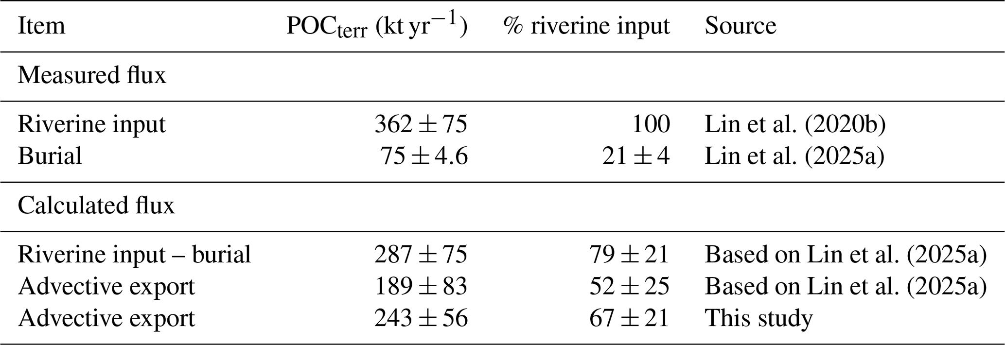
Combining POC_terr concentrations with simulated flow data (Fig. C5), we estimated an advective flux of 243±56 kt yr⁻¹ from the northeastern Taiwan Strait, providing a first-order approximation for the magnitude of POC_terr export. This value is broadly consistent with the regional imbalance between riverine input and burial (Table 1) and may help close the POC_terr budget. It is higher than our previous estimate that accounted for benthic oxidation (Lin et al., 2025a), although the two values likely overlap within uncertainties.

Table 1 POC_terr budget of the northeastern Taiwan Strait.

Notably, 48 % of exported POC_terr exited via waters above the narrow (< 10 km) nearshore mud belt, underscoring its dual role as both a temporary sink of fluvial inputs and a source fuelling long-distance transport. An additional 36 % was exported via the nepheloid layer above the offshore mud belt, whereas only 17 % was carried by clear shelf waters. However, as discussed above, POC_terr concentrations in low-TSM samples are likely underestimated by the lignin-based approach. If the sixfold correction derived from the average Λ8${}_{\mathrm{cal}}/\mathrm{\Lambda }$8_terr,s ratio is applied, the contribution of clear shelf waters would increase to 43 %. This suggests that low-TSM shelf waters, though having a minor fraction of terrigenous OM, may play a non-negligible role in its advective transport.

5.2 Controlling factors of marine POM properties

We first compared POM characteristics before and after correction for terrigenous input. Here, “overall characteristics” refer to slopes derived from linear regressions of variables. The measured and corrected overall atomic C $/$ N ratios were 7.67±0.16 and 6.56±0.15, respectively, and differed significantly (p<0.0001). Excluding high-TSM samples yielded comparable values (6.87±0.15 and 6.61±0.16; p= 0.08; Fig. 6a). After correction, overall POC $/$ Chl ratios decreased from 92.7±18.4 to 79.6±10.9 g C g⁻¹ Chl, and for low-TSM samples from 91.8±9.8 to 83.0±9.1 g C g⁻¹ Chl (Fig. 6b). These differences were not significant (p= 0.15 to 0.16). Neither did the correction alter the δ¹³C_OC-temperature relationship for low-TSM samples.

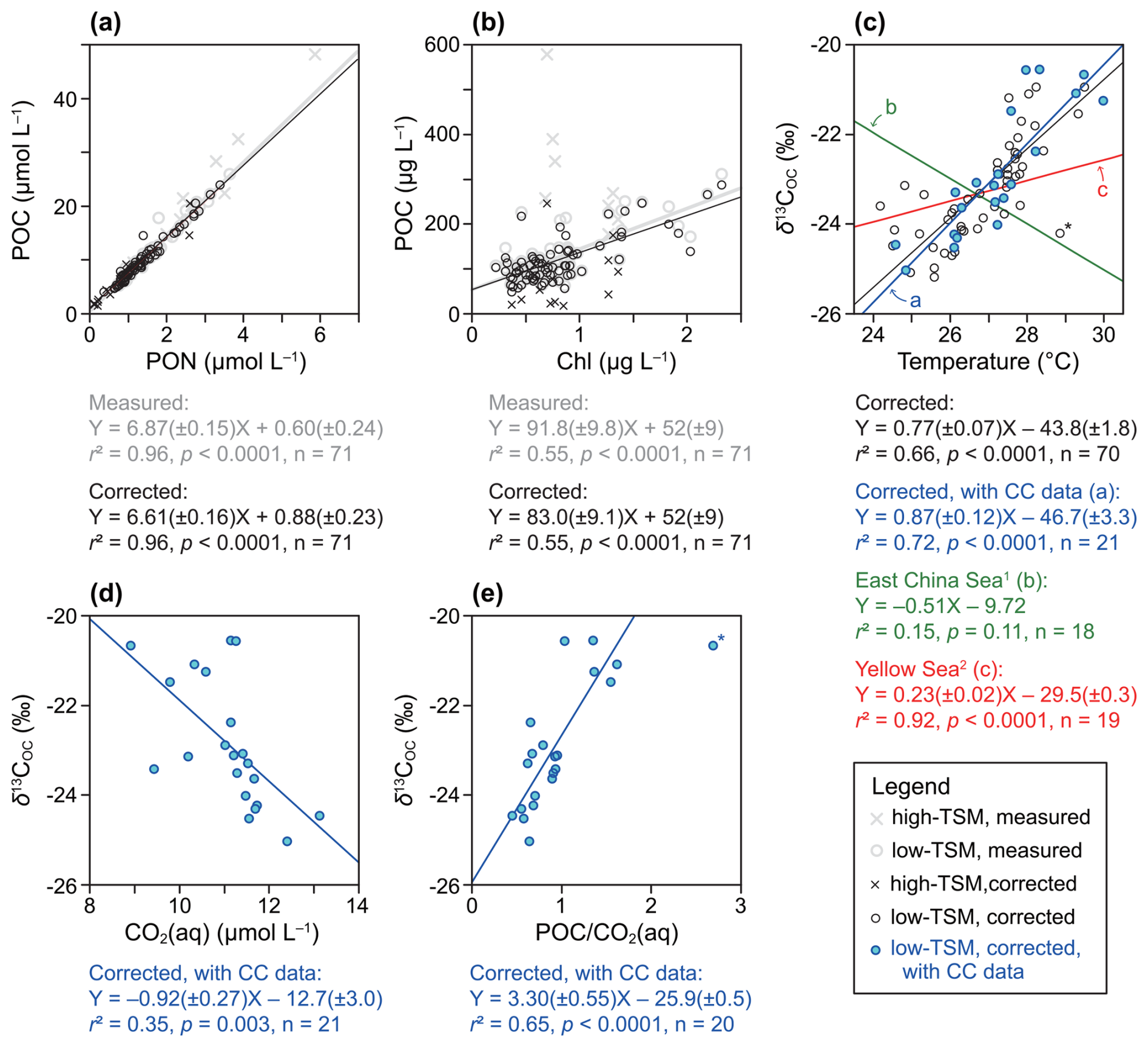
Figure 6 Characteristics of marine POM. (a) Relationship between POC and PON. (b) Relationship between POC and Chl. (c) Relationship between δ¹³C_OC and temperature. (d) Relationship between δ¹³C_OC and CO₂(aq). (e) Relationship between δ¹³C_OC and POC $/$ CO₂(aq) (both in µmol L⁻¹). Linear regressions are based on low-TSM samples only. ^* denotes data excluded from the regression. References: 1 = Liu et al. (2018a); 2 = Liu et al. (2022).

As discussed in Sect. 5.1.2, the lignin-based approach likely underestimates POC_terr, which may partly contribute to the limited differences observed after correction. However, even when accounting for the potential magnitude of this underestimation, terrigenous POM remains a secondary component in low-TSM samples. The weak correlations between POC and Σ8 (r= 0.14, p= 0.27) and between δ¹³C_OC and Λ8 ($r=-\mathrm{0.04}$, p= 0.76) in these samples further indicates that additional upward revision of lignin-based POC_terr estimates is unlikely to substantially alter the slopes of linear regressions used to assess overall characteristics. In the following discussion, we therefore focus on the corrected low-TSM dataset, while noting that the conclusions are insensitive to whether the correction is applied.

5.2.1 C $/$ N ratios reflect nutrient supply ratios

The overall C $/$ N ratio of 6.61±0.16 (Fig. 6a) agrees with the global median of 6.5 (Martiny et al., 2013) and canonical Redfield ratio of 6.63, with no offshore-nearshore difference (p= 0.09). Regionally, our values resemble those from summer POM in the upper 200 m at SEATS in the South China Sea (6.44±0.28; p= 0.48; Liu et al., 2007; Fig. 1a), but exceed those of the DCM in the East China Sea (5.76±0.14; p<0.0001; Liu et al., 2018a). Further north, the Yellow Sea DCM values (6.31±0.53; Liu et al., 2022) are indistinguishable from our results (p= 0.12). Although phytoplankton C $/$ N ratios are influenced by nutrients, irradiance, temperature, growth rate, and community structure, nutrient supply remains the dominant control in the global surface ocean (Moreno and Martiny, 2018; Tanioka and Matsumoto, 2020). Marine primary production is commonly N-limited in the world ocean, but N stress is alleviated in large plume-affected regions (Huang et al., 2019). This mechanism was invoked to explain lower POM C $/$ N ratios in the western North Atlantic (Martiny et al., 2013). Across the Pan-China Sea (cf. Bianchi et al., 2018), C $/$ N variation is consistent with this pattern. Near Redfield ratios prevail in the South China Sea, Taiwan Strait, and Yellow Sea, where nutrient supply is relatively balanced (Huang et al., 2019; Liu et al., 2022; Wong et al., 2015), whereas lower ratios occur in the East China Sea owing to nitrogen enrichment from the Yangtze River (Zhong et al., 2025).

5.2.2 POC $/$ Chl ratios track photoacclimation

Cellular OC $/$ Chl ratio is a physiological indicator of phytoplankton growth constraints (Arteage et al., 2014; Gui and Sun, 2024). It responds to light, nutrients, and temperature, although temperature effects are minor at regional scales (Wang et al., 2009). When light intensity is strong, phytoplankton down-regulates Chl synthesis to prevent damage from excess light and reallocates resources towards carbon fixation, elevating the ratio. With increasing water depth, the ratio decreases as cells invest nitrogen in light harvesting (Brown et al., 2003; Li et al., 2010). Under high nitrogen availability, more nitrogen is allocated to light harvesting, lowering the ratio; under nitrogen limitation, nitrogen is diverted to enzymes needed for nutrient acquisition, increasing the ratio (Arteage et al., 2014). The ratio also underpins conversions from satellite Chl to phytoplankton carbon biomass (Carr et al., 2006). Microscopy and flow cytometry, along with assumptions of cell geometry and empirical equations for cellular carbon content, are the standard approaches to estimate phytoplankton carbon biomass required to compute OC $/$ Chl ratio (e.g., Li et al., 2010). Here, we explore whether overall POC $/$ Chl ratios can approximate phytoplankton OC $/$ Chl ratios in shelf waters by comparing our values with cell-based estimates and model predictions.

The regression between POC and Chl shows a non-zero intercept (Fig. 6b), indicating contributions from detritus or heterotrophs. The overall POC $/$ Chl ratio of 83.0±9.1 g C g⁻¹ Chl is close to the OC $/$ Chl value of nutrient-depleted surface waters (∼ 90 g C g⁻¹ Chl; Eppley, 1968) and lies with the modeled range of 50–100 g C g⁻¹ Chl for the nitrogen-limited subtropical western North Pacific (Arteage et al., 2014).

Two sample subsets showed elevated Chl concentrations and merit further examination: nearshore waters and offshore DCM layers (Fig. 3d). Nearshore waters, enriched by riverine nitrogen input in summer (1–3 µmol L⁻¹ nitrate plus nitrite; Huang, 2022), had a ratio of 75.0±12.5 g C g⁻¹ Chl (Fig. C6a). Offshore DCM layers, which are nitrogen-depleted (< 1 µmol L⁻¹ nitrate; Tseng et al., 2020), showed a lower ratio of 43.0±29.1 g C g⁻¹ Chl, although the POC-Chl relationship was not significant (Fig. C6b). This contrast is further supported by comparisons of measured POC $/$ Chl ratios, which are higher in nearshore waters than in offshore DCM layers (p<0.001). Overall POC $/$ Chl ratios as low as 28–38 g C g⁻¹ Chl have been reported for DCM layers in the East China Sea and Yellow Sea (Liu et al., 2018a, 2022). The pattern observed in our samples indicates that photoacclimation exerts a stronger control on the POC $/$ Chl ratio than nutrient stress, based on the physiological considerations described above. Alternative explanations include shifts in phytoplankton community composition, as suggested by Li et al. (2010), or covariation between bacterial biomass and Chl, as demonstrated by Brown et al. (2003). Given the highly dynamic nature of planktonic communities in shelf waters, we refrain from relate our POC $/$ Chl data to reported variability in community composition in the Taiwan Strait (e.g., Tong et al., 2024; Zhong et al., 2020). Concurrent measurements of POM properties and planktonic community structure are therefore required to robustly resolve the mechanisms underlying POC $/$ Chl ratio.

5.2.3 Temperature control on δ¹³C_OC

δ¹³C of marine phytoplankton reflects the balance between growth demand and DIC supply in seawater (Fry, 1996). Under diffusive CO₂ transport, isotopic fractionation between CO₂ and cellular carbon increases when growth slows or CO₂(aq) concentration rises (i.e., a lower μ $/$ CO₂(aq) ratio, where μ is growth rate), producing more negative δ¹³C (Laws et al., 1995). Biological parameters influencing fractionation include growth rate (Laws et al., 1995), cell geometry (Popp et al., 1998) and taxonomic physiology (Burkhardt et al., 1999), whereas relevant environmental factors include CO₂(aq), nutrients (Riebesell et al., 2000), and temperature (Rau et al., 1989). When CO₂(aq) is low, many phytoplankton activate carbon concentrating mechanisms (CCMs; Giordano et al., 2005), which reduce fractionation (Fielding et al., 1998; Sharkey and Berry, 1985) and weaken the predictability of δ¹³C based on μ $/$ CO₂(aq) ratios (Burkhardt et al., 1999; Rau et al., 2001). A critical CO₂(aq) concentration of ∼ 10 µmol L⁻¹ to induce CCMs has been suggested as the threshold for CCM induction, although CCMs may operate at concentrations above this level (Burkhardt et al., 1999).

Because δ¹³C of DIC varies little in the global euphotic zone (Kroopnick, 1985) and the temperature effect on the variation of bicarbonate-CO₂(aq) isotopic equilibrium is small (0.12 ‰ K⁻¹; Mook et al., 1974), δ¹³C_OC of POM largely reflects biological fractionation. Globally, δ¹³C_OC decreases toward higher latitudes, a trend attributed to increased CO₂ solubility in colder waters (Rau et al., 1989). Recent work by Liu et al. (2022) showed that temperature is a better predictor of POM δ¹³C_OC than either CO₂(aq) or POC $/$ CO₂(aq) ratio, a proxy for the μ $/$ CO₂(aq) ratio, in both shelf and open ocean environments. This is possibly because temperature integrates multiple biological and environmental controls on isotopic fractionation, irrespective of carbon acquisition modes (Liu et al., 2022).

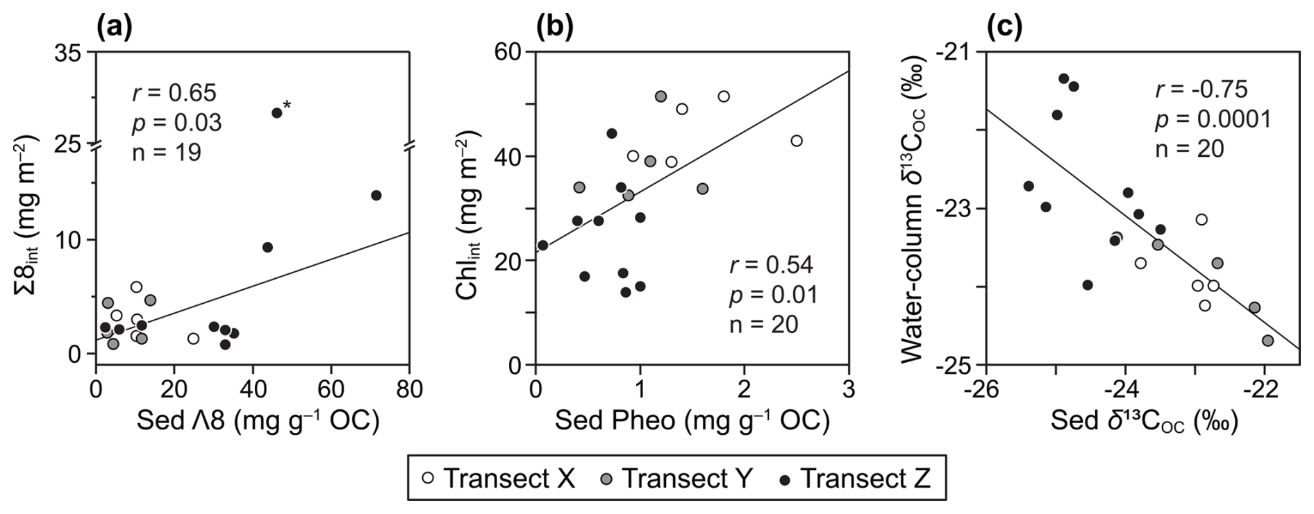
Figure 7 Comparison of POM and sedimentary OM. (a) Water-column integrated Σ8 (Σ8_int) versus OC-normalized lignin concentration (Λ8) of the sediments (Sed). (b) Water-column integrated Chl (Chl_int) versus sedimentary OC-normalized pheopigments a (Pheo) concentration. (c) POC-weighted water-column δ¹³C_OC versus sedimentary δ¹³C_OC.

Our dataset corroborates this view. Across all samples, δ¹³C_OC correlates strongly with temperature (Fig. 6c). For samples with carbonate chemistry data, the r² values follow the order temperature (0.72), POC $/$ CO₂(aq) ratio (0.65), and CO₂(aq) (0.35) (Fig. 6c to e), confirming temperature as the strongest predictor. The weak CO₂(aq) relationship likely reflects widespread CCM activity in the warm, high-light conditions of our study area. Comparisons with the East China and Yellow Seas show no clear regional trend in slope (Fig. 6c), limiting broader extrapolation. Even so, for regional POM studies, this relationship provides a practical constraint on the isotopic composition of marine POM (Fig. 2) and improves estimates of terrigenous POC in the water column (Sect. 3.3.2).

5.3 Comparison of POM and sedimentary OM

Differences between water-column POM and underlying sedimentary OM have long interested researchers studying particle transport, carbon preservation, and paleoenvironmental reconstruction (Hayes et al., 1999; Wakeham and McNichol, 2014; Wang et al., 2017). Concomitant measurements of POM and surface sediment OM from the Taiwan Strait (Lin et al., 2025a) allow us to assess how short-term hydrogeochemical signals in POM compare with the sedimentary archive of this shelf environment. We examined three categories of parameter pairs: (i) water-column integrated Σ8 versus sedimentary lignin, (ii) water-column integrated Chl versus sedimentary photosynthetic pigments, and (iii) POC-weighted water-column δ¹³C_OC versus sedimentary δ¹³C_OC. Sediment data represent the upper 1 cm, reflecting recent deposition. For categories (i) and (ii), all relevant variants of sedimentary parameters reported in Lin et al. (2025a), including dry-weight concentration, OC-normalized concentration, and burial flux, were included. Sedimentary pigments comprise Chl and pheopigments a, derivatives of Chl formed during biological degradation (Stephens et al., 1997; Sun et al., 1993).

Correlation coefficients for all parameter pairs are listed in Table A7, and the best-correlated pair in each category is shown in Fig. 7. Water-column integrated stocks showed the strongest correlations with OC-normalized sedimentary biomarker concentrations. For lignin (Fig. 7a), the correlation reflects the role of seabed sediment as a major lignin source to the water column (Sect. 5.1.1) and indicates that lignin-rich sedimentary OM likely contains easily resuspended wood microdetritus. For photosynthetic pigments (Fig. 7b), Lin et al. (2025a) attributed the relationship to the biological pump. Notably, nearshore “hot spots” of photosynthetic activity, characterized by high POC, heavy δ¹³C_OC and low CO₂(aq) (Fig. 4), did not dominate the correlation; instead, sedimentary patterns were primarily controlled by euphotic-zone thickness, which also governs depth-integrated primary production in the region (Tseng et al., 2020).

By contrast, δ¹³C_OC in POM and sedimentary OM shows a puzzling negative correlation (Fig. 7c). Because δ¹³C_OC integrates OM from sources with distinct isotopic signatures, the result points to the competing influences of lateral and vertical transport in shaping sedimentary δ¹³C_OC on shallow shelves. The absence of a positive relationship between sedimentary and water-column δ¹³C_OC, together with the temperature dependence of marine POM δ¹³C_OC, raises a fundamental question: Is it appropriate to assign a single marine δ¹³C_OC endmember in isotope mixing models? Previous work suggests that incorporation of marine POM into sediments largely occurs during episodic, high-POC pulses (Berger and Wefer, 1990) with minimal isotopic fractionation (Kukert and Riebesell, 1998). Yet in environments where blooms are rare, as is likely the case in parts of the northeastern Taiwan Strait, the isotopic signatures of marine OM ultimately buried on the seafloor remain poorly constrained. Revisiting published datasets containing δ¹³C_OC of co-sampled suspended, sinking and deposited particles, along with hydrographic context, may help address this issue.

6 Conclusions

This study provides an integrated, full-water-column assessment of terrigenous and marine POM in the northeastern Taiwan Strait. The results demonstrate how hydrodynamics, water-mass structure, resuspension, and primary production jointly regulate POM sources, distribution, and export on this energetic shelf. The main findings are:

Lignin tracers reveal contributions from both Taiwanese rivers and the Pearl River plume. POC_terr was estimated using a two-step approach that incorporated both lignin and δ¹³C_OC data. Terrigenous fractions are low in low-TSM waters but rise sharply in high-TSM layers due to sediment resuspension.

Combining POC_terr with HYCOM velocities yields an export flux of ∼ 243±56 kt C yr⁻¹, comparable to the mismatch between riverine supply and sedimentary burial. This flux helps close the regional POC_terr budget.

After correction for terrigenous contributions, C $/$ N ratios reflect balanced nutrient supply, POC $/$ Chl ratios respond to photoacclimation, and δ¹³C_OC is better explained by temperature than CO₂(aq)-related variables, implying widespread CCM activity.

Sedimentary lignin and pigment concentrations correspond to their water-column stocks, but the negative POM-sediment δ¹³C_OC correlation shows that lateral transport overprints vertical delivery in determining sedimentary isotopic composition.

Overall, this work refines the quantification of terrigenous and marine POM, clarifies source-to-sink connectivity, and strengthens the modern framework needed to interpret sedimentary OM proxies in shelf environments.

Appendix A

Table A1 List of sampling sites from the cruise NOR3-0104.

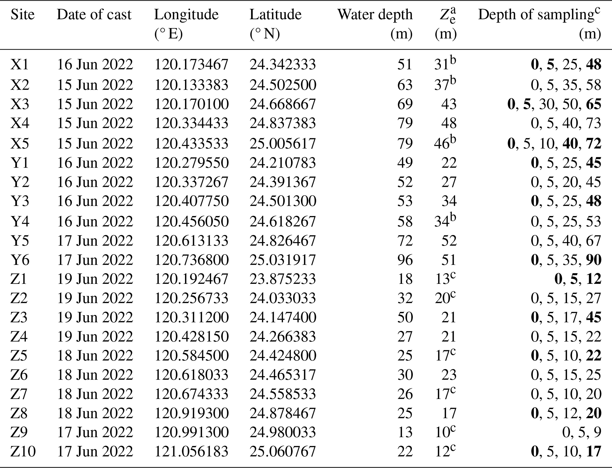
^a Z_e is the euphotic zone depth, defined as the depth of 1 % of surface photosynthetically active radiation. ^b denotes values derived from the linear regression between measured Z_e and bottom-water depth (Eq. 3). ^c Bold depths indicate subsampling depths for carbonate chemistry analysis.

Table A2 Inferred sources of terrigenous OM and results of the lignin-based estimation.

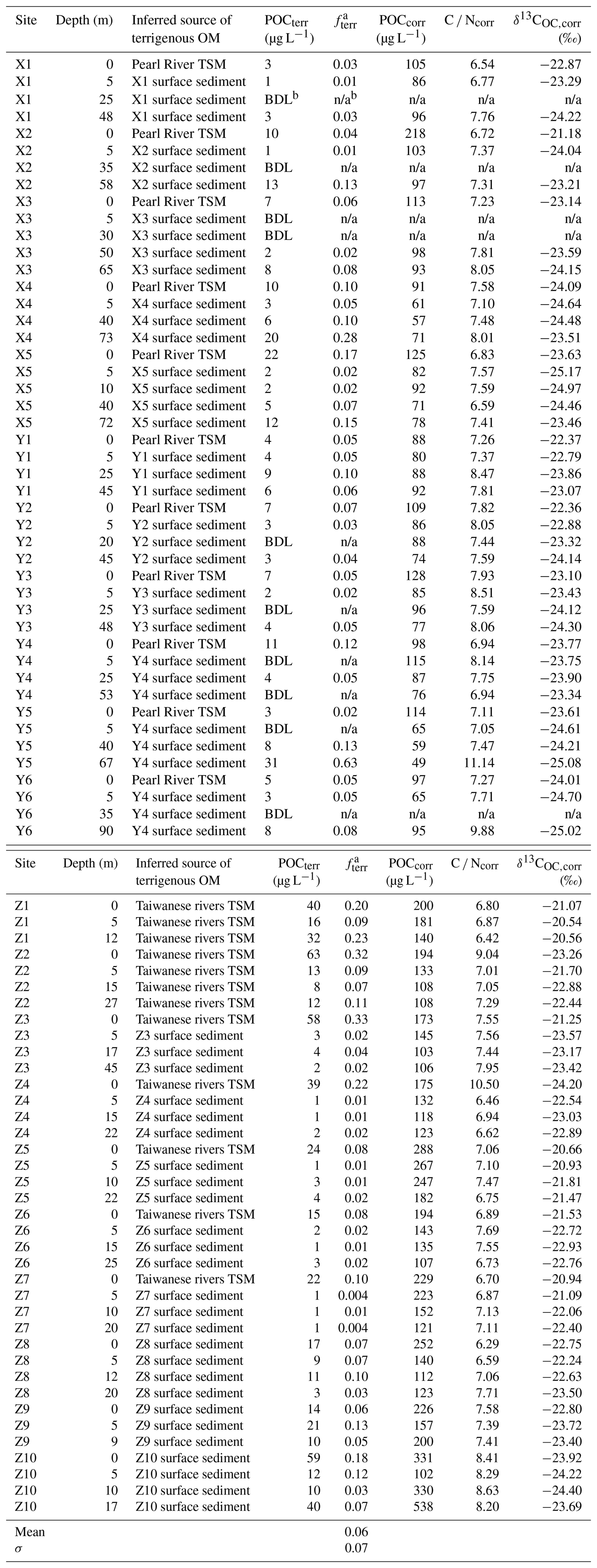
^a Fractional contribution of POC_terr to measured POC. ^b BDL, below detection limit of lignin; n/a, not applicable.

Table A3 Geochemical properties of potential terrigenous OM sources. Unless otherwise noted, data are from Lin et al. (2025a). n/a – not applicable.

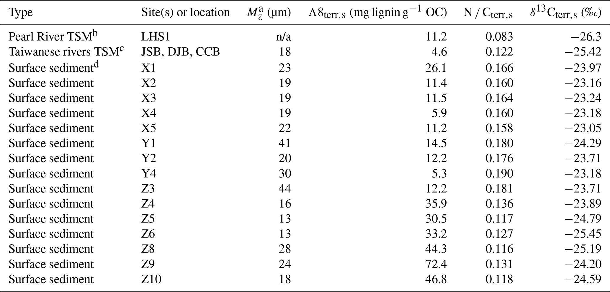
^a Mean grain size. ^b For Pearl River TSM, Λ8_terr,s, N $/$ C_terr,s, and δ¹³C_terr,s are equal to the measured values (Zhang et al., 2014). ^c For Taiwanese rivers TSM, Λ8_terr,s was calculated using Λ8 = 0.0490 × $Q_{\mathrm{w}}^{\mathrm{0.9847}}$ (r²= 0.94, n= 7; derived from Lin et al., 2025a), where Q_w is the fluvial water discharge (∼ 100 m³ s⁻¹ prior to and during the cruise NOR3-0104). N $/$ C_terr,s and δ¹³C_terr,s are taken from measured values. ^d For seabed sediments of the northeastern Taiwan Strait, these parameters were derived from the output of the mixing models presented in Lin et al. (2025a).

Table A4 Endmember values and results of the binary mixing model for high-TSM (≥ 4 mg L⁻¹) samples.

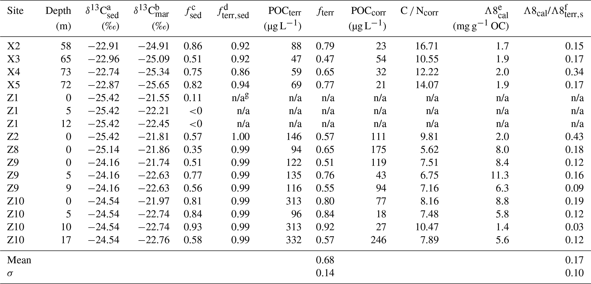
^a Site-specific endmember δ¹³C values of sedimentary OC, taken from measured values reported in Lin et al. (2024). ^b Temperature-dependent endmember δ¹³C values of marine OC (cf. Sect. 5.2.3). ^c Sedimentary fraction of POC. ^d Terrigenous fraction of sedimentary OC, taken from the mixing model outputs presented in Lin et al. (2025a). ^e Calculated source Λ8 signatures (Eq. 6) that account for the measured Λ8 of the high-TSM samples. ^f Λ8_terr,s values are taken from Table A3. ^g n/a, not applicable.

Table A5 Data sources and parameter settings used for the CO2SYS computations.

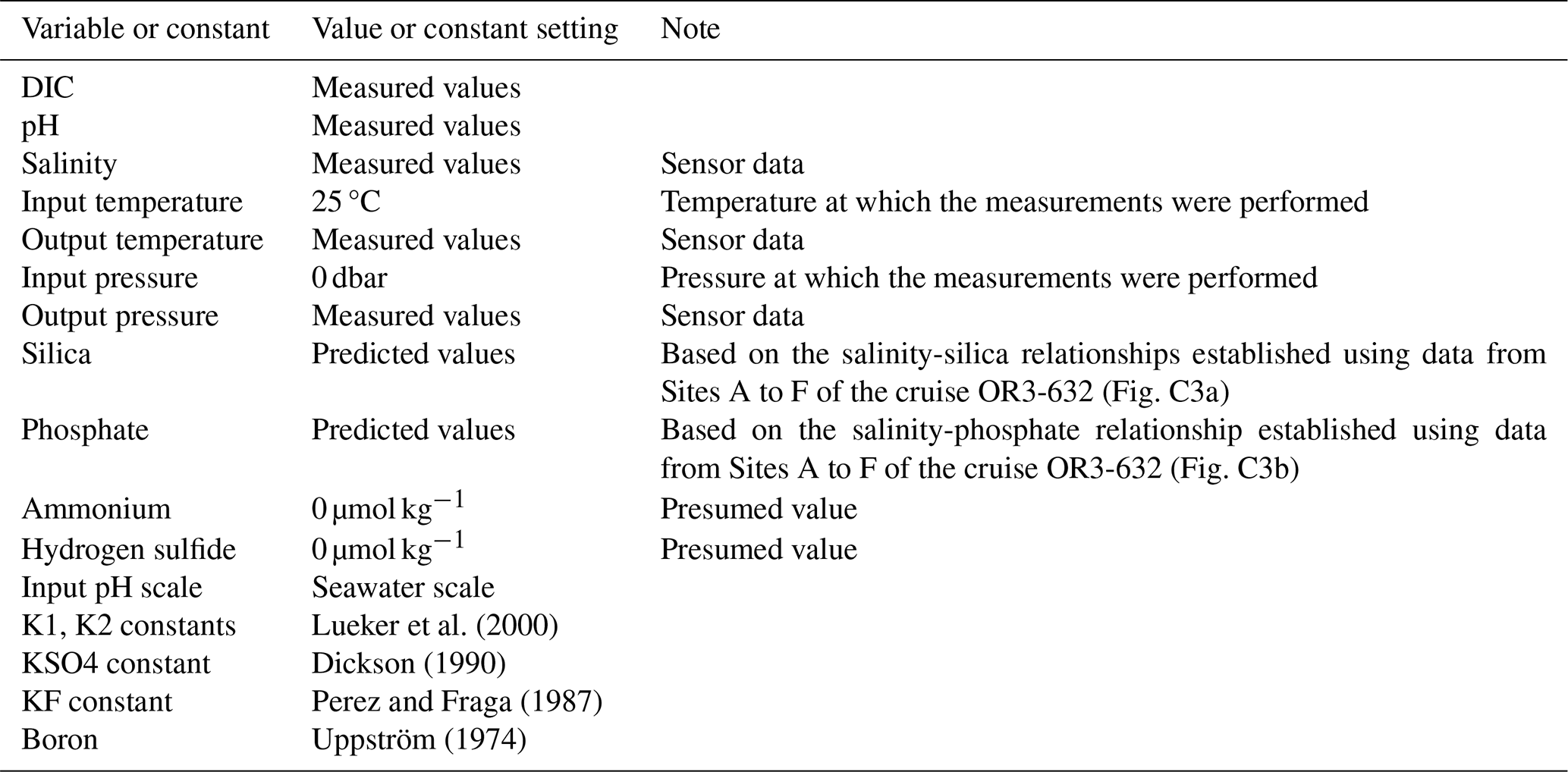
Table A6 CO₂(aq) concentrations computed using the CO2SYS program.

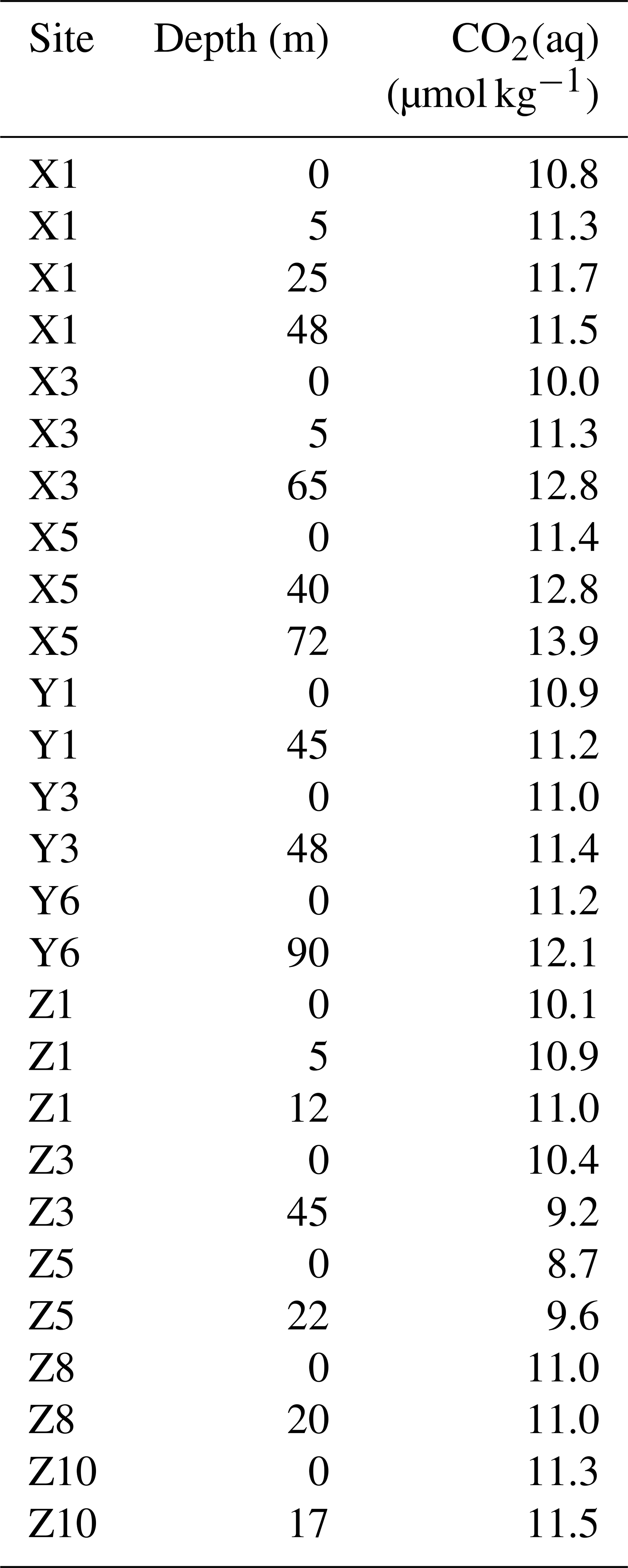
Table A7 Correlation^a between water-column and sedimentary OM parameters.

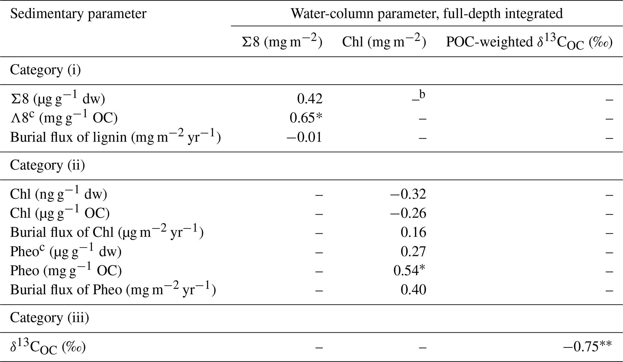
^a Values in bold indicate strong correlations (r≥0.7 or $\le -\mathrm{0.7}$). ${}^{**}$ and ^* denote significance at the 0.01 and 0.05 levels, respectively. ^b Not applicable. ^cΛ8, OC-normalized concentration of eight lignin monomers; Pheo, pheopigments a.

Appendix B

B1 Lignin-based estimation of POC_terr

Lignin is a powerful biomarker for diagnosing the relative abundance of terrigenous OM. Its use for quantifying POC_terr, however, is not straightforward and relies on two assumptions: (i) Λ8_terr remains constant during transport and sorting from source regions to shelf waters, and (ii) particulate lignin experiences negligible alteration (e.g., dissolution or oxidation). Observations in our samples that may challenge these assumptions, and their implications for POC_terr quantification, are discussed in Sect. 5.1.2.

After deriving POC_terr with Eq. (4), we calculated POC, N $/$ C, and δ¹³C_OC corrected for terrigenous inputs using following mixing equations:

$$\begin{array}{}\text{(B1)}& {\displaystyle }{\mathrm{POC}}_{\mathrm{corr}}={\mathrm{POC}}_{\mathrm{m}}-{\mathrm{POC}}_{\mathrm{terr}}\text{(B2)}& {\displaystyle }\begin{array}{rl}& {\left(\mathrm{N}/\mathrm{C}\right)}_{\mathrm{corr}}\\ & =\left[{\mathrm{POC}}_{\mathrm{m}}\times {\left(\mathrm{N}/\mathrm{C}\right)}_{\mathrm{m}}-{\mathrm{POC}}_{\mathrm{terr}}\times {\left(\mathrm{N}/\mathrm{C}\right)}_{\mathrm{terr},\mathrm{s}}\right]/{\mathrm{POC}}_{\mathrm{corr}}\end{array}\text{(B3)}& {\displaystyle }\begin{array}{rl}& {\mathit{\delta }}^{\mathrm{13}}{\mathrm{C}}_{\mathrm{OC},\mathrm{corr}}\\ & =\left({\mathrm{POC}}_{\mathrm{m}}\times {\mathit{\delta }}^{\mathrm{13}}{\mathrm{C}}_{\mathrm{OC},\mathrm{m}}-{\mathrm{POC}}_{\mathrm{terr}}\times {\mathit{\delta }}^{\mathrm{13}}{\mathrm{C}}_{\mathrm{terr},\mathrm{s}}\right)/{\mathrm{POC}}_{\mathrm{corr}}\end{array}\end{array}$$

where subscripts m and corr denote measured and corrected values for POM, respectively, and s refers to the inferred source material.

B2 Binary mixing model with floating endmembers for estimating POC_terr of high-TSM samples

We applied a δ¹³C-based binary mixing model that treats POC as a mixture of sedimentary (sed) and marine (mar) sources:

$$\begin{array}{}\text{(B4)}& {\displaystyle }{f}_{\mathrm{sed}}+f_{\mathrm{mar}}=\mathrm{1}\text{(B5)}& {\displaystyle }{f}_{\mathrm{sed}}\times {\mathit{\delta }}^{\mathrm{13}}{\mathrm{C}}_{\mathrm{sed}}+f_{\mathrm{mar}}\times {\mathit{\delta }}^{\mathrm{13}}{\mathrm{C}}_{\mathrm{mar}}={\mathit{\delta }}^{\mathrm{13}}{\mathrm{C}}_{\mathrm{OC},\mathrm{m}}\end{array}$$

where f is the fractional contribution of each OC component to bulk POC. Endmember δ¹³C values (Table A4) vary spatially for δ¹³C_sed and with temperature for δ¹³C_mar. Some samples produced negative f_sed values (Table A4), likely reflecting uncertainties in the δ¹³C_OC-temperature relationship. Samples with f_sed near or below zero were grouped with low-TSM samples for evaluation of marine POM. f_sed values above 0.3 were used to calculate POC_terr (Eq. 5), which was further used to derive POC_corr, N $/$ C_corr, and Λ8_cal (Eqs. B1, B2, and 6; Table A4).

B3 Estimating the advective POC_terr flux out of the northeastern Taiwan Strait

We defined a latitudinal transect at 25.04° N (120.40–121.04° E; Fig. 1b) as the northern boundary of the study area and quantified the export flux as the rate of material crossing this transect.

A previous study of nutrient fluxes through the Taiwan Strait (Huang et al., 2019) used polynomial regressions linking measured concentrations to observed temperature and salinity, which were then related to HYCOM outputs of temperature and salinity. This approach was not suitable for POC_terr because of sparse data coverage and weak regression performance (r²<0.3; data not shown). Instead, we used POC_terr concentrations derived from summer samples to calculate the annual flux. Interpolation along the transect used measurements from Sites X5, Y6, Z9, and Z10. To restrict sediment resuspension to the known offshore and nearshore mud belts, dummy stations were added at the belt margins (Fig. 1b) and assigned the POC_terr value of Site Y6. Because our sampling took place under calm sea states, resuspension was likely mild, making the flux estimate conservative. Although simplified, the approach is sufficient for comparing the export flux with riverine inputs from Taiwan.

Flow rates along the transect were obtained from HYCOM, which provides $\mathrm{1}/\mathrm{12}$° horizontal resolution and 41 vertical layers. Daily east-west (u) and north-south (v) velocity data for 2022 were averaged to derive the annual mean velocity ($\stackrel{\mathrm{‾}}{u}$,  $\stackrel{\mathrm{‾}}{v}$) used in flux estimation.

Interpolation of POC_terr and flow speed was carried out using the Data Interpolating Variational Analysis (DIVA) function in Ocean Data View (Fig. C5). Outputs were exported as 1 km × 1 m grid cells using the 2-D estimation function. The export flux (F) of each grid cell was calculated as:

$$\begin{array}{}\text{(B6)}& F={\mathrm{POC}}_{\mathrm{terr}}\times A\times \sqrt{{\stackrel{\mathrm{‾}}{u}}^{\mathrm{2}}+}{\stackrel{\mathrm{‾}}{v}}^{\mathrm{2}}\end{array}$$

A is the area of the grid cell. Figure C5c shows the resulting cross section of POC_terr export flux. The total flux was obtained by summing across all grid cells. The uncertainty was propagated from known sources, including analytical errors in POC (3 %) and lignin (20 %), as well as uncertainty in the δ¹³C_OC-temperature relationship (11 %).

Appendix C

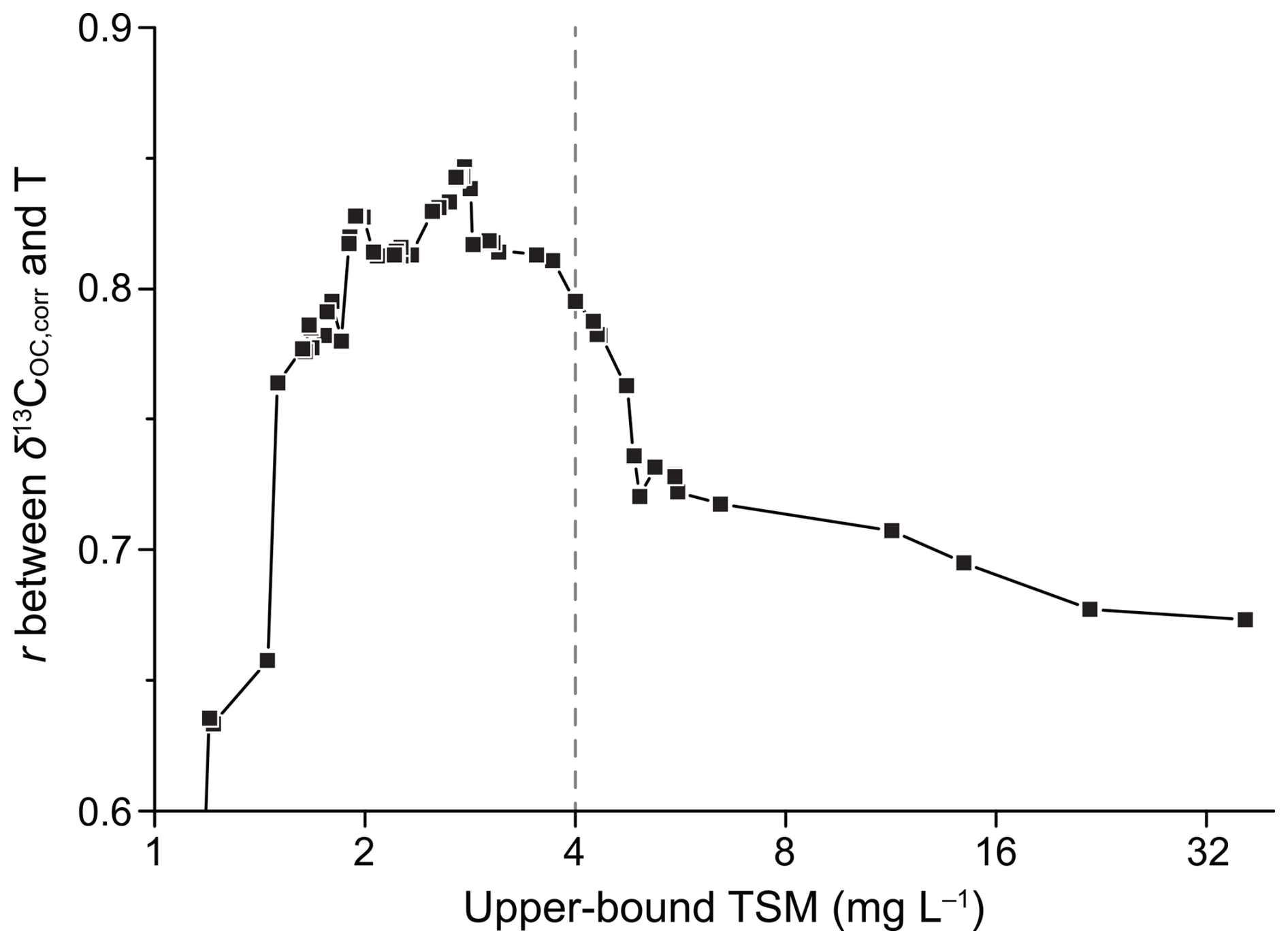
Figure C1 Correlation between δ¹³C_OC,corr (from Step 1) and temperature (T) versus the upper-bound TSM in each data subset. The correlation coefficient declined sharply when TSM exceeded 4 mg L⁻¹, so this value (dashed gray line) was used to separate low- and high-TSM samples.

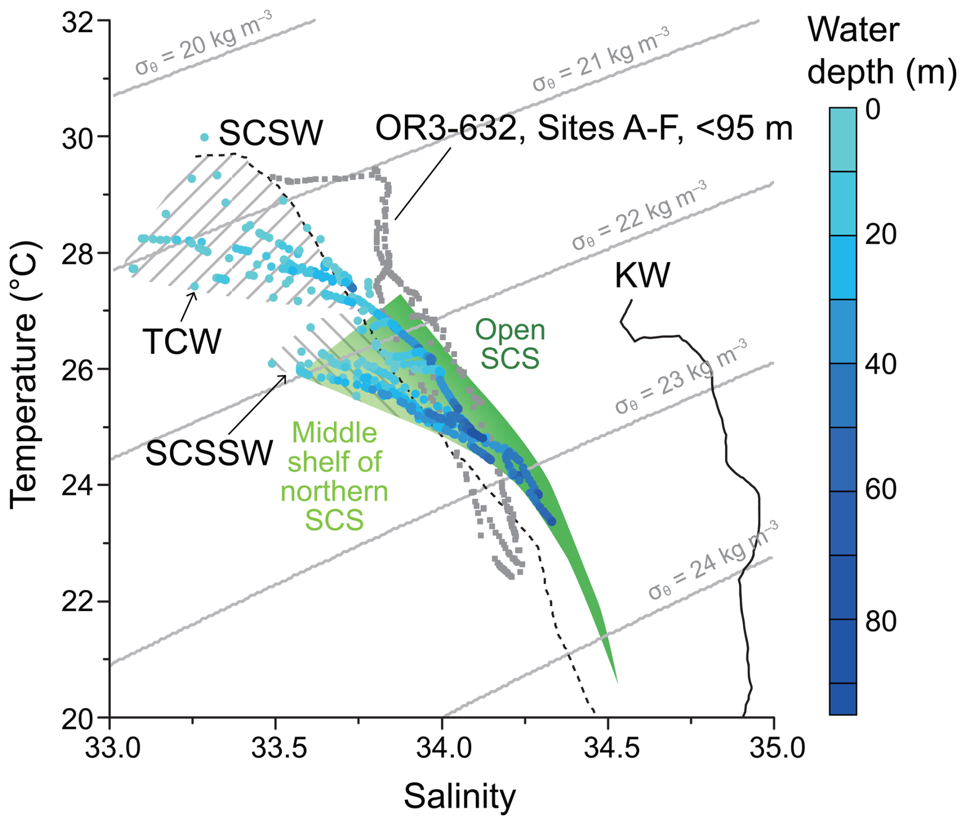
Figure C2 Depth-referenced T–S diagram for the NOR3-0104 sampling sites in the northeastern Taiwan Strait. Characteristic summer T–S properties of South China Sea Water (SCSW) and Kuroshio Water (KW) were digitized from Jan et al. (2010). For comparison, T–S properties from Sites A to F of cruise OR3-632 and from Transect T1 (green shade; Wong et al., 2015) are also shown. Light green indicates water properties characteristic of middle-shelf stations in the northern South China Sea (SCS), whereas dark green represents those of open SCS. Samples with salinity lower than typical SCSW values were divided into two groups, one referred to as the Taiwan Coastal Water (TCW) and the other associated with the characteristics of South China Sea Surface Water (SCSSW).

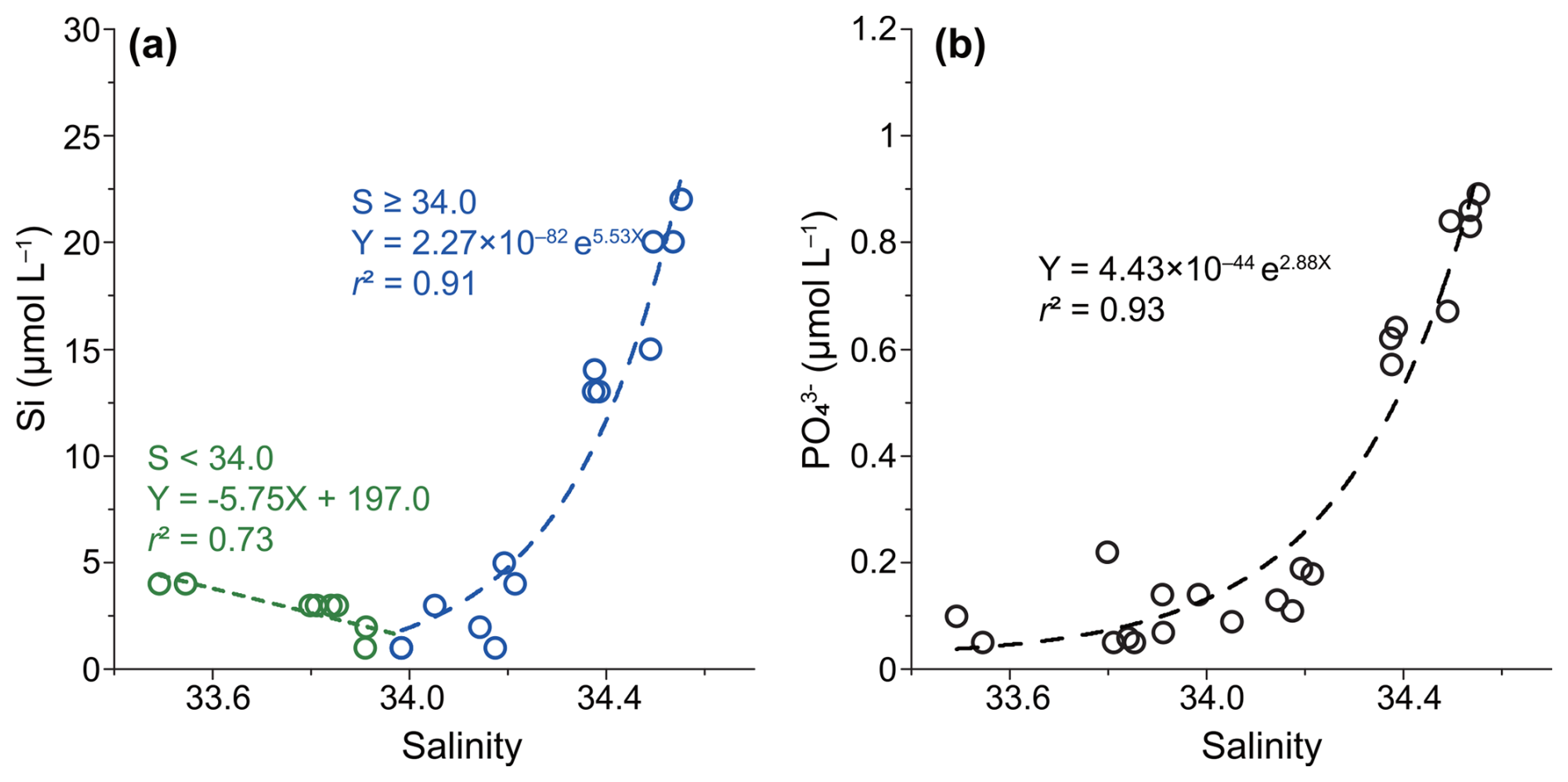
Figure C3 Salinity-based empirical relationships used to predict silica and phosphate concentrations. (a) Salinity-silica relationships. (b) Salinity-phosphate relationship. Data from Sites A to F of the cruise OR3-632.

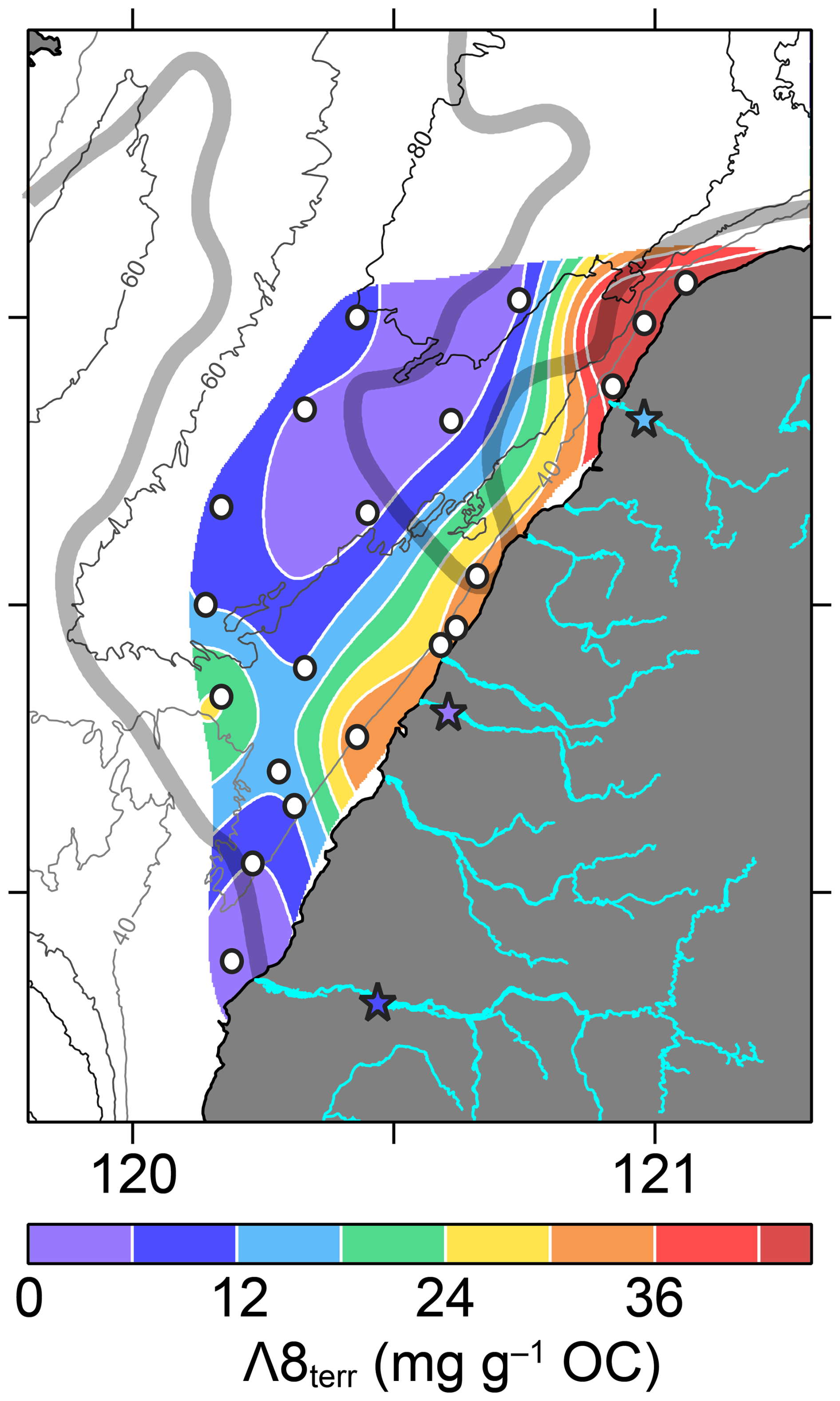
Figure C4 Spatial distribution of Λ8_terr in seabed sediments of the northeastern Taiwan Strait. White dots mark marine sediment sampling sites, and riverine TSM data (stars) are also shown with colors matching the legend. The thick gray line denotes the boundary (mean grain size = 63 µm; Fig. 1b) of mud belts. Data from Lin et al. (2025a).

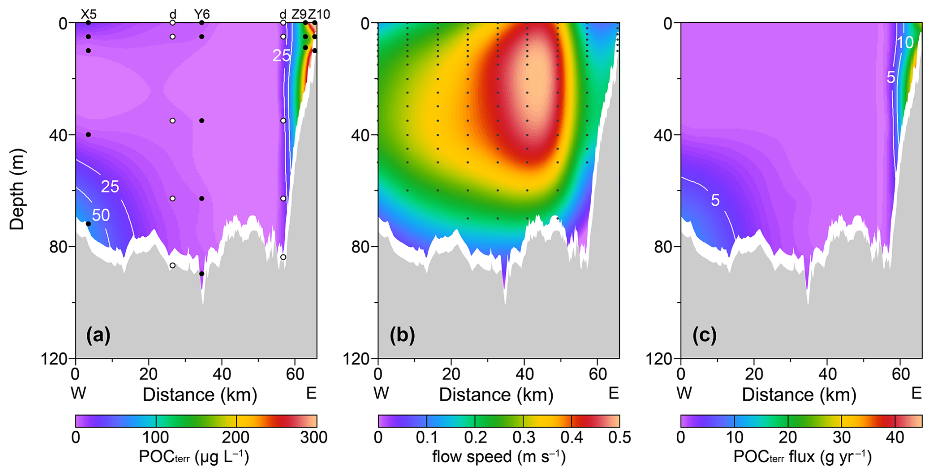
Figure C5 Data used for estimating the POC_terr export flux. (a) POC_terr concentration. Black and white dots are CTD samples and dummy (labeled with d above the frame) stations, respectively. (b) Annual mean flow speed, with black dots marking HYCOM grid points. (c) Calculated POC_terr export flux from the northeastern Taiwan Strait. The bottommost 5 m of the water column were excluded from the calculation.

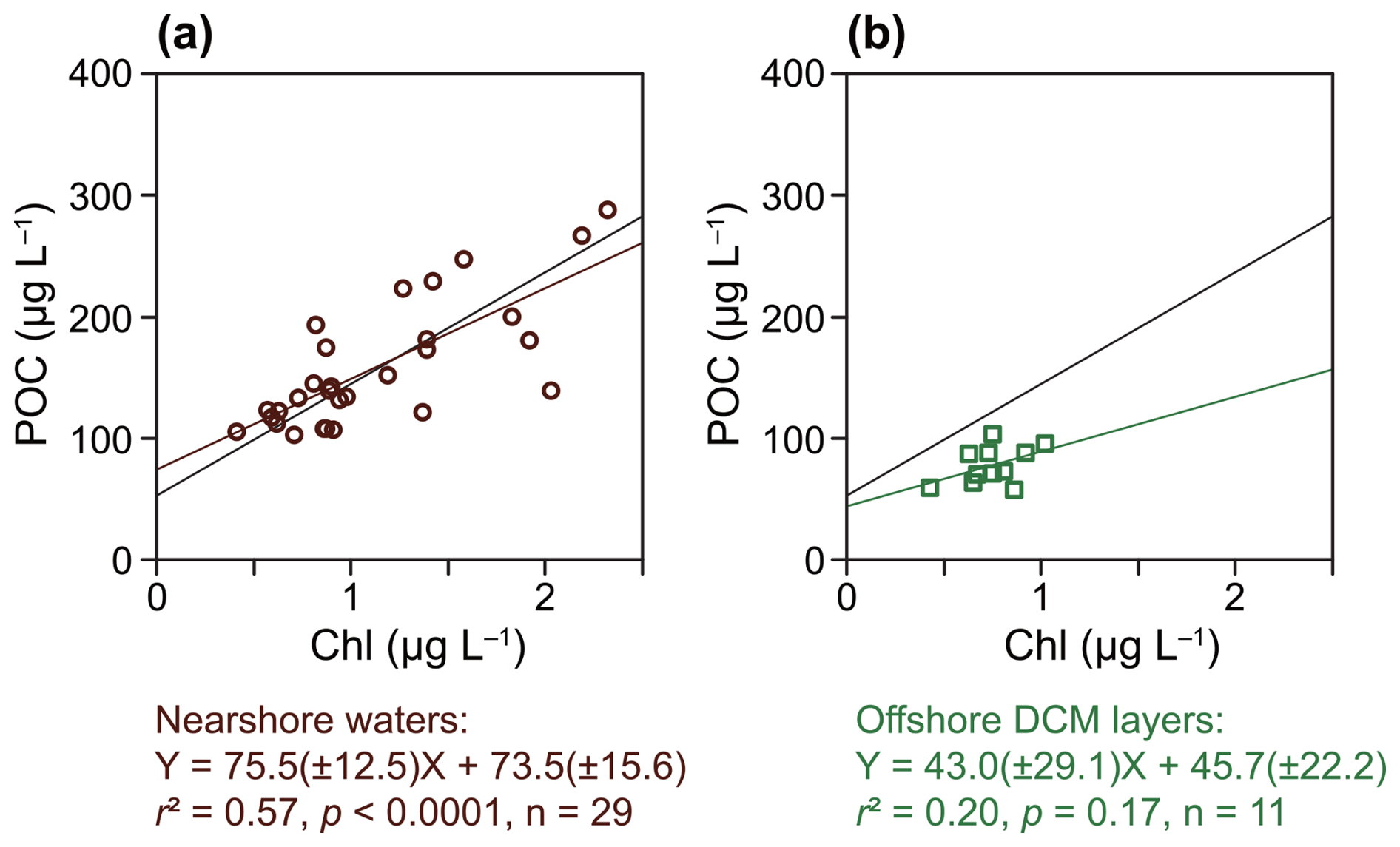
Figure C6 POC-Chl relationships for different sample subsets. (a) Nearshore samples. (b) Offshore samples from the DCM layers. The black line denotes the POC-Chl relationship of low-TSM samples, as shown in Fig. 6b.