Evaluating a multispectral miniaturised fluorometer with three excitation channels for predicting phytoplankton community structure indices from BGC-Argo float observations

Phytoplankton community composition is a key determinant of ocean biogeochemical cycles, yet its observation from autonomous platforms remains challenging. In this study, we assessed the potential of in situ multispectral excitation fluorescence (MXF) to predict phytoplankton community structure indices in the Northwestern Mediterranean Sea. With a view toward applications on Biogeochemical-Argo (BGC-Argo) profiling floats, we evaluated a miniaturised, three-excitation-channel fluorometer. Laboratory measurements on ten phytoplankton strains confirmed that MXF ratios at 440, 470, and 532 nm provide taxon-specific signatures, especially for picocyanobacteria and green algae. Field observations of phytoplankton pigments were clustered into four ecologically distinct phytoplankton communities across the seasonal cycle, which defined the targeted phytoplankton community structure indices. A machine learning model was then trained to classify these clusters using MXF and additional bio-optical indices. Results show that existing BGC-Argo configurations (single-wavelength fluorescence, particulate backscattering, and beam attenuation coefficients) reliably distinguish broad community structures, such as pico- versus microphytoplankton dominance, but resolving finer pigment-based differences requires the additional spectral information provided by MXF. The different excitation channels contributed unequally: 440 and 470 nm provided robust pigment sensitivity across communities, while 532 nm was particularly informative for detecting phycoerythrin-rich taxa. Overall, combining MXF with bio-optical proxies improved classification performance by integrating pigment-specific and size-structure information, demonstrating the potential of MXF to enhance autonomous monitoring of phytoplankton community dynamics and their role in ocean biogeochemical cycles.

1 Introduction

Phytoplankton play a key role in global biogeochemical cycles, particularly in the carbon cycle. They fix dissolved inorganic carbon through photosynthesis and transfer a portion of it to higher trophic levels, initiating the biological carbon pump. This mechanism is pivotal in regulating the ocean's carbon storage. However, primary production, i.e., the rate at which phytoplankton produce organic carbon, varies significantly across different time and space scales. This variation is attributed to environmental changes that induce changes in phytoplankton community structure and biomass (Rousseaux and Gregg, 2014). Therefore, in the current context of climate change, monitoring phytoplankton dynamics on a global scale is crucial.

The emergence of new observation platforms, such as Biogeochemical-Argo (BGC-Argo) profiling floats equipped with miniaturised bio-optical sensors, offers the possibility to collect continuous vertical profiles of optical measurements that serve as proxies of biogeochemical variables (Biogeochemical-Argo Planning Group, 2016; Claustre et al., 2020). Fluorescence is a widely used proxy of chlorophyll a (Chl a) concentration, a ubiquitous pigment in phytoplankton organisms, which is in turn used as an indicator of phytoplankton biomass. Equipped with (single channel) fluorometers, autonomous platforms thus allow the observation of phytoplankton biomass variability across a wide range of spatial and temporal scales (e.g. Boss et al., 2008; Barbieux et al., 2019; Cornec et al., 2021; Bock et al., 2022).

Information on phytoplankton biomass only, however, is insufficient to understand the links between phytoplankton and the carbon cycle. Indeed, the composition of phytoplankton communities is known to be a critical determinant of the carbon cycle since several key processes largely vary between phytoplankton size classes or phylogenetic groups, such as CO₂ fixation through photosynthesis (Cermeño et al., 2005; Uitz et al., 2008), trophic interactions (Cushing, 1989; Finkel, 2007), elemental cycling (Morel 2008, Litchman et al., 2015), or carbon transfer to the deep ocean (Buesseler et al., 1998; Guidi et al., 2009; Henson et al., 2012; Bonnet et al., 2023).

Yet, the composition of phytoplankton communities cannot be measured directly from the sensors currently implemented on BGC-Argo floats. Only a few methods have been proposed so far to overcome this challenge and go beyond the mere estimation of Chl a biomass from bio-optical measurements of BGC-Argo floats. Specifically, Sauzède et al. (2015) developed a neural network algorithm using the vertical shape of the in situ fluorescence profile as input to retrieve the relative contribution to the Chl a of the three phytoplankton size classes (pico-, nano- and microphytoplankton). Cetinić et al. (2015) proposed a simple community index based on the ratio of the fluorescence signal to the particulate backscattering coefficient. Similarly, Terrats et al. (2020) used this ratio to detect coccolithophore blooms. Finally, Rembauville et al. (2017) developed a regional approach to estimate the stock of particulate organic carbon (POC) of bacteria and three phytoplankton size classes. This approach has been developed for applications to BGC-Argo floats that measure not only the fluorescence and particulate backscattering coefficient, but also the beam attenuation coefficient. More recently, Brewin et al. (2022) proposed an analytical framework to partition vertical chlorophyll profiles measured by BGC-Argo floats into contributions from two phytoplankton communities associated with the mixed layer and the deep chlorophyll maximum, combining chlorophyll and particulate backscattering observations. This model was later extended to three communities in an oxygen minimum zone context (Cox et al., 2023). Yet, while those methods provide useful information about phytoplankton community composition, they mostly rely on regional empirical relationships between phytoplankton community composition and bio-optical indices.

Multispectral excitation fluorescence (MXF) is an alternative approach to retrieve information on the relative pigment composition of the phytoplankton assemblage, from which major taxa can be discriminated. MXF consists in measuring in situ fluorescence signals in response to excitation at different wavelengths, corresponding to the absorption peaks of different accessory pigments used as biomarkers of specific taxa in the phytoplankton community (e.g. Yentsch and Phinney, 1985; Bricaud et al., 2004; Brewin et al., 2014). A combination of three wavebands centred around 440, 470 and 532 nm was previously investigated in freshwater environments (Proctor and Roesler, 2010) and in the Arabian Sea (Thibodeau et al., 2014), providing promising results and paving the way for use in open ocean waters. Multi-channel instruments such as the FluoroProbe (bbe Moldaenke, 5 excitation wavelengths) have also been widely used for in situ taxonomic discrimination in freshwater and coastal environments (Beutler et al., 2002; Catherine et al., 2012). More recently, multi-wavelength excitation fluorometer applications have extended to open ocean discrimination of phytoplankton assemblages, demonstrating their capacity to resolve major taxonomic groups including diatoms, dinoflagellates, as well as phycoerythrin-containing (Synechococcus, Trichodesmium, etc.) or lacking (Prochlorococcus) cyanobacteria (Xu et al., 2022; Kodama et al., 2022). Concurrently, laboratory-based studies have demonstrated that portable, low-cost multi-excitation devices combined with machine learning classifiers can achieve high-accuracy taxonomic discrimination across a wide range of phyla (Magalhães et al., 2025; Zhang et al., 2025), further highlighting the potential of this approach for scalable, cost-effective phytoplankton monitoring.

The present study aims at extending the approach of Proctor and Roesler (2010) and assessing the potential of in situ three-excitation-channel MXF as a proxy of phytoplankton taxonomic composition in view of future applications to BGC-Argo floats. Higher-resolution multispectral fluorometers, such as the FluoroProbe and MultiExciter (9 channels), offer enhanced taxonomic discrimination (e.g., Garrido et al., 2019; Kodama et al., 2022; Xu et al., 2022). However, their significant weight, large physical footprint, and high-power consumption limit their use primarily to shipboard or short-term logging applications. In contrast, the SeaBird ECO sensor used in the present study is miniaturised and optimised for the stringent power and payload constraints of the global BGC-Argo fleet (Bittig et al., 2019). Our study therefore evaluates whether a reduced 3-channel spectral subset sensor, ready for integration on profiling floats, can provide sufficient biological resolution for global-scale autonomous observations.

Although standard BGC-Argo floats are all equipped with a single-channel fluorometer (with excitation at 470 nm) and a backscattering sensor (e.g., Bittig et al., 2019), part of the BGC-Argo fleet is also instrumented with additional sensors that may provide useful information on phytoplankton composition indicators, such as a beam transmissometer (Rembauville et al., 2017) or a dual-channel fluorometer with excitation around 440 and 470 nm. Of note, the nominal wavelength of the blue excitation channel is sometimes referred to as 435 nm in instrument metadata (see https://vocab.nerc.ac.uk/collection/R27/current/, last access: 2 July 2026) but both values correspond to the same blue excitation band used in these fluorometers.

In this context, the present study aims to evaluate the potential of bio-optical measurements from the sensors currently implemented on BGC-Argo profiling floats, either alone or in combination with MXF, for retrieving information on phytoplankton community composition. Hence, we designed a predictive machine learning model to assess the ability of MXF combined with other bio-optical observations to infer taxonomic information. For this purpose, we combined laboratory experiments and fieldwork conducted in the Northwestern (NW) Mediterranean Sea. The NW Mediterranean Sea provides a good case study because its pronounced seasonal phytoplankton biomass cycle (e.g., D'Ortenzio et al., 2005; Lavigne et al., 2015) and ecological succession (Marty et al., 2002; Mayot et al., 2017) are comparable to those observed in the temperate regions of the open ocean.

For the laboratory work, we selected ten phytoplankton strains representative of the various taxa observed along the seasonal succession of the NW Mediterranean Sea. We measured the MXF response of each strain under controlled conditions and measured the variability among taxa and strains. This allowed us to characterise the MXF sensor and validate the analysis of the field data. During our fieldwork, we collected concomitant pigment concentrations and bio-optical parameters using a sensor package comprising a MXF sensor, a single-channel fluorometer, a backscatterometer and a transmissometer over an annual cycle in the NW Mediterranean Sea. This in situ dataset was then used to develop and test a phytoplankton community composition discrimination model. Ultimately, we provide recommendations for the use of MXF, alone or in combination with other bio-optical indicators, to infer the taxonomic composition of phytoplankton communities from BGC-Argo profiling float observations.

2 Material and methods

2.1 Laboratory work

2.1.1 Phytoplankton strains and culture conditions

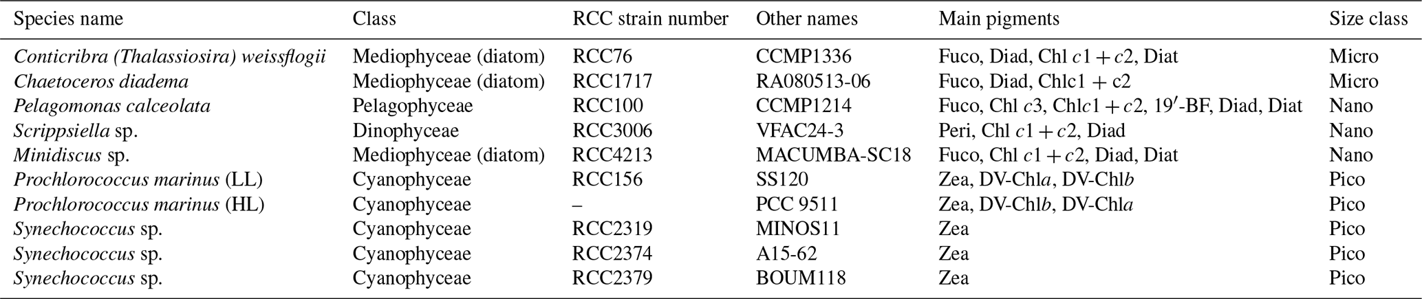
For laboratory experiments, we selected ten phytoplankton strains provided by the Roscoff Culture Collection (RCC; https://roscoff-culture-collection.org/, last access: 2 July 2026). These strains were selected as being representative of the taxonomic diversity of the main eukaryotic and prokaryotic phytoplankton organisms encountered in open-ocean waters, and particularly at the BOUSSOLE site in the NW Mediterranean Sea, based on previous pigment-based studies in the region (Marty et al., 2002; Mayot et al., 2017). The selected strains include three diatom species, one Pelagophyceae, one dinoflagellate and five photosynthetic prokaryotes (three Synechococcus and two Prochlorococcus strains; Table 1).

Table 1 Name, taxonomy, pigment composition as detected by High Performance Liquid Chromatography (HPLC) pigment analysis, and size class of the ten phytoplankton strains used for the laboratory experiments. Pico for picophytoplankton (0.2–2 µm), Nano for nanophytoplankton (2–20 µm) and Micro for microphytoplankton (20–200 µm); HL stands for high-light adapted; LL stands for low-light adapted. The pigments measured are chlorophyll a (Chl a), fucoxanthin (Fuco), diadinoxanthin (Diad), diatoxanthin (Diat), 19^′-hexanoyloxyfucoxanthin (19^′-HF), 19^′-butanoyloxyfucoxanthin (19^′-BF), peridinin (Peri), zeaxanthin (Zea), divinyl-chlorophyll a and b (DV-Chla, DV-Chlb), chlorophyll c1 and c2 or c3 (Chlc1 + c2, Chlc3).

All strains were grown at a constant temperature of 21 °C, under 50 µmol photons m⁻² s⁻¹ continuous white light provided by a white-blue-green LED system (Alpheus, France), and in either K + Si (Keller et al., 1987) or PCR-S11 culture medium (Rippka et al., 2000) for eukaryotes and prokaryotes, respectively. As fluorescence is significantly influenced by the physiology of phytoplankton cells, we used cultures in stable physiological status as assessed by a high PSII quantum yield (F_v $/$ F_M) using a Phyto-PAM-II fluorometer (Walz, Effeltrich, Germany). The F_v $/$ F_M parameter was calculated as (F_M− F₀) $/$ F_M (Pittera et al., 2014), where F₀ is the dark-adapted basal fluorescence, F_M is the maximal fluorescence associated with the closing of photosynthetic reaction centres, and F_v is the variable fluorescence. F_M was measured after exposure to saturating light pulses and addition of 100 µM of the photosystem II inhibitor 3^′-(3,4-dichlorophenyl)-1^′,1^′-dimethylurea (DCMU; Parkhill et al., 2001). The F_v $/$ F_M parameter was measured concomitantly to cell counts made using a Guava EasyCyte flow cytometer (Luminex Corporation, USA) all over the growth of each phytoplankton culture (Marie et al., 2001). The MXF protocol (see Sect. 2.1.2) was applied to each culture in the middle to late exponential growth phase, before the drop of the F_v $/$ F_M index. The MXF protocol was repeated three times on distinct replicate culture vessels for each strain (biological triplicates).

2.1.2 Multispectral fluorescence measurements

All MXF measurements were performed using an ECO 3X1M fluorometer (Sea-Bird electronics, USA), with three excitation wavebands centred onto 440, 470, and 532 nm, and emission onto 695 nm, with a 10 nm bandwidth. This three-channel design has been chosen for its immediate capacity to be integrated on a BGC-Argo float, or equivalent autonomy asset, due to its miniaturisation and low power consumption, the ECO series sensor already being part of the BGC-Argo payload. To determine the fluorescence to Chl a slope factor (here expressed in fluorescence per Chl a unit), the MXF measurements were collected for each culture over a 5-point dilution series ranging from 0.1 to 10 mg Chl a m⁻³. Each culture was dark acclimated for 2 h before dilution and MXF measurements. The MXF measurements were performed immediately after dilution to avoid any dilution-induced physiological stress. The ECO 3X1M sensor outputs were recorded with the TeraTerm^® software. Each culture was diluted in a 1 L glass beaker that was then placed under constant slow stirring. The multispectral fluorometer was placed at the centre of the beaker, and the optical window was immersed 5 mm below the surface. Blank measurements were performed with culture media and were then subtracted from the culture measurements to remove any possible fluorescence signal from coloured dissolved organic matter. Blank values were within a few counts of the dark reading, indicating that the measurements were not subject to optical interferences from the beaker edge or benchtop scattering. For each culture triplicate, on each dilution, we measured the fluorescence response during three series of one minute of continuous acquisition at 1 Hz, each separated by two minutes of darkness. The signal did not decrease significantly during acquisition, indicating that there was no quenching during the protocol application. The ECO 3X1M was used with factory calibration coefficients. Temperature effects on the sensor were considered negligible as only the optical window was immersed in the culture medium, and never for more than one minute continuously. The stability of the signal over each one-minute acquisition period confirmed the absence of any thermal drift.

2.1.3 Laboratory data processing

For each of the ten selected phytoplankton strains grown in culture, the MXF measurements were processed as follows. First, for each dilution series, a blank value was recorded by measuring the average response of the culture medium alone and was then subtracted from the raw sensor output acquired for the culture as described above. The MXF measurements collected over the three consecutive acquisition periods were averaged to obtain a single fluorescence value, expressed in digital counts (DC). Finally, the dilution series was used to define a Chl a-specific calibration value, expressed in units of DC (mg Chl a m⁻³)⁻¹, for each of the three excitation wavelengths and each of the ten selected strains. This calibration value represents the coefficient of a linear regression between the fluorescence response at a given wavelength expressed in DC and the Chl a concentration in mg m⁻³ for the entire dilution range and for each replicate of a given phytoplankton strain. For the sake of simplicity, the raw fluorescence signal, in DC, at an excitation wavelength λ, will be noted as F_λ (i.e., F₄₄₀, F₄₇₀, and F₅₃₂ for the excitation wavelengths 440, 470, and 532 nm, respectively) and the Chl a-specific calibration value will be noted as F${{}^{\ast }}_{\mathit{\lambda }}$ (i.e., F${{}^{\ast }}_{\mathrm{440}}$, F${{}^{\ast }}_{\mathrm{470}}$, and F${{}^{\ast }}_{\mathrm{532}})$.

2.2 Field measurements of bio-optical and biogeochemical variables

2.2.1 Sampling strategies

Concomitant phytoplankton pigment determinations and bio-optical measurements were performed at sea every month, from December 2020 to October 2021 at the BOUSSOLE station (Buoy for the acquisition of long-term optical time series), a long-term monitoring site located at 7°54^′E, 43°22^′N in the Ligurian (NW Mediterranean) Sea (Antoine et al., 2008). On each monthly cruise (Golbol et al., 2000), a CTD-rosette equipped with an optical sensor package was used to perform casts from the surface down to 400 m depth. The optical package included an MXF sensor (the same ECO 3X1M as used for the laboratory experiments), an ECO FLBB sensor, and a C-Rover beam transmissometer (both Sea-Bird Scientific). The ECO FLBB measures the Chl a fluorescence at one excitation (470 nm) and one emission (695 nm) wavelengths, as well as the particulate backscattering coefficient at 700 nm (b_bp; see Sect. 2.2.2). It is worth noting that among the three excitation channels of the ECO 3X1M (440, 470, and 532 nm), the first two (440 and 470 nm) are shared with the two types of dual-channel fluorometers (Sea-Bird Scientific ECO FLBBFL or RBR Tridente) currently implemented on some BGC-Argo floats. This correspondence allows us to also test the potential of dual-channel fluorometers for inferring phytoplankton composition indicators in our analysis. The C-Rover transmissometer measures the light beam transmitted between the emitter and receptor (at 650 nm and over an optical path length of 25 cm), allowing the calculation of the attenuation coefficient. From this, the particulate beam attenuation coefficient (c_p) is calculated by removing the attenuation of pure seawater. Both sensors have already been mounted on several BGC-Argo floats for different biogeochemical applications (e.g., Mignot et al., 2014; Rembauville et al., 2017; Barbieux et al., 2022). Concomitantly, seawater was sampled from the Niskin bottles attached to the CTD-rosette at ten discrete depths for pigment identification and quantification by HPLC.

2.2.2 In situ data processing

The factory-determined dark value of the ECO FLBB sensor was validated in the laboratory using black tape to cover the optical window, then subtracted from the raw DC following BGC-Argo data management recommendations (Schmechtig et al., 2018a). The optical backscattering coefficient was measured during the CTD-rosette upcast, which was used for seawater sampling. The angular scattering coefficient (β) was recorded every second at a central angle of 124° and a wavelength of 700 nm. To obtain the particulate angular scattering coefficient (β_p), the contribution of pure water, dependent on temperature and salinity (Zhang et al., 2009), was subtracted from β. The β_p coefficient was then converted into b_bp following standard conversion guidelines and applying a χ factor of 1.076 (Schmechtig et al., 2018b).

The ECO 3X1M sensor was mounted on the CTD-rosette frame, providing simultaneous MXF measurements. The same black tape procedure was used to subtract dark values. The raw fluorescence values, expressed as counts, were directly used as the fluorescence signal. The particulate attenuation coefficient was corrected for sensor drift and calculated from total beam transmittance as in Barnes and Antoine (2014). The outliers in fluorescence, c_p and b_bp datasets were detected and removed using a threshold of 1.5 simple moving average (Δ depth =3 m). Each profile was then smoothed using a simple moving average (Δ depth =3 m).

2.3 Determination of phytoplankton pigments

For both laboratory and field samples, Chl a and accessory pigments were identified and quantified by HPLC analysis. Briefly, seawater from discrete field samples (∼ 2 L) or cultures (0.1 to 0.5 L, depending on culture biomass concentration) was filtered onto glass fibre filters (GF/F Whatman 25 mm), stored in liquid nitrogen during cruises and then transferred at −80 °C in the laboratory until further analysis at the SAPIGH HPLC analytical facility of the Institut de la Mer de Villefranche (IMEV). Phytoplankton pigments were extracted by sonication in 3 mL methanol (100 %) at −20 °C for 2 h clarified by vacuum filtration (GF/F Whatman 25 mm), and finally analysed within 24 h by HPLC using an Agilent Technologies 1200 Series system. More details about the analytical protocol can be found in Ras et al. (2008). The total chlorophyll a concentration, [Chl a], is defined as the sum of chlorophyll a, divinyl-chlorophyll a , and chlorophyllid a concentration.

For in situ samples, we specifically investigated the distribution of seven diagnostic pigments (DP): peridinin (Peri), 19^′-butanoyloxyfucoxanthin (19^′-BF), fucoxanthin (Fuco), 19^′-hexanoyloxyfucoxanthin (19^′-HF), alloxanthin (Allo), zeaxanthin (Zea), divinyl-chlorophyll a (DV-Chla), divinyl-chlorophyll b (DV-Chlb), and chlorophyll b (Chl b), with total chlorophyll b (TChlb) defined as the sum of DV-Chlb and Chl b. These pigments are defined as biomarkers of major phytoplankton taxa and were further grouped into three phytoplankton size classes, i.e. micro- (> 20 µm), nano- (2–20 µm) and picophytoplankton (< 2 µm), according to the approach of Claustre (1994) and Vidussi et al. (2001). Following the equations given in Uitz et al. (2006), the DP-based method allowed the estimation of the relative contribution to the [Chl a] of the three size classes. Because it relies on biomarker pigment concentrations, this approach yields an average, synthetic estimate of both the taxonomic and size composition of the phytoplankton communities. Although it has limits because some phytoplankton taxa may occasionally span over several size classes and some DP may be found in several taxa (e.g. Vidussi et al., 2001; Chase et al., 2020), this approach provides a widely used information about the phytoplankton community structure at large spatial and temporal scales (e.g., Vidussi et al., 2001; Bricaud et al., 2004; Uitz et al., 2006; Brewin et al., 2014). Moreover, the BOUSSOLE site and the NW Mediterranean Sea have been the subject of extensive prior characterisation of phytoplankton seasonal dynamics (e.g., Marty et al., 2002; Organelli et al., 2013; Latasa et al., 2022), providing a well-documented ecological context against which the outputs of this method can be interpreted.

2.4 Statistical analyses

To explore the potential of deriving phytoplankton community composition from MXF and other bio-optical measurements, we employed a two-step analytical approach.

First, we derived phytoplankton community indices, defined as clusters with similar pigment composition. Phytoplankton pigment data were analysed using Correspondence Analysis (CA) to identify similarities in pigment composition among samples. The first three dimensions of the CA were then subjected to a Hierarchical Ascending Classification (HAC) to define distinct clusters, corresponding to typical phytoplankton assemblages observed in the NW Mediterranean at the BOUSSOLE site (following Kramer and Siegel, 2019; Uitz et al., 2023).

Then, these clusters were used as categorical targets to evaluate the ability of MXF and bio-optical descriptors to infer phytoplankton composition through a Histogram Gradient Boosting (HGB) classification model.

This clustering-based strategy offers three key advantages: (1) it reduces the number of target variables, effectively adapting to the reduced number of degrees of freedom imposed by the limited number of excitation channels; (2) it transforms the prediction task from a regression to a classification problem, reduces the direct influence of biomass magnitude and allows the model to focus solely on taxonomic composition indices; and (3) it ensures that the model captures the most significant source of taxonomic variability in the dataset, thereby reducing the influence of minor variance components and mitigating the risk of overfitting. All analyses were carried out in R (v4.3.1; R Core Team) and Python (v3.14). Data processing, quality control, and the correspondence-analysis clustering were performed in R using the tidyverse, vegan, and FactoMineR packages, with figures produced via ggplot2, patchwork, and ggpubr. The machine-learning classification was implemented in Python with scikit-learn (v1.8.0) and imbalanced-learn (v0.14.1), supported by pandas, NumPy, Matplotlib, and seaborn.

2.4.1 Correspondence analysis

We used CA to visualise the main similarities among samples based on their relative pigment concentrations. This method generates linear combinations of relative pigment contributions, creating a new multidimensional space where sample projections reflect their resemblance in pigment composition.

In this transformed space, samples with similar pigment signatures are located close to each other, while those with distinct compositions are further apart. The first dimensions of the analysis capture the most significant variance in the dataset, effectively summarising the dominant patterns in pigment distribution. By reducing data complexity, this approach provides a clearer interpretation of how different phytoplankton communities are structured based on their pigment signatures.

We applied this statistical method for two key objectives. First, we used it to compare the pigment composition of cultured phytoplankton strains with that of field samples, assessing whether the selected strains accurately represent the seasonal phytoplankton succession at the sampled location in the NW Mediterranean Sea. This CA was performed using the seven DP concentrations from the experiment samples. Field samples were then projected in the transformed CA projection space, and the distance between field and laboratory samples will be discussed. Second, we conducted a CA exclusively on field samples, using the same set of pigments, and extracted the first three components as inputs for our clustering method described hereafter.

2.4.2 Clustering of phytoplankton pigment data

The pigment data from NW Mediterranean field samples, consisting of the set of pigment concentrations detailed in the previous section, were clustered to identify major phytoplankton assemblages along the seasonal cycle using the CA (cf. Sect. 2.4.1). The first three dimensions of the CA were used to quantify the resemblance in pigment composition across samples. A Hierarchical Ascending Classification (HAC) was then applied to these three dimensions, grouping samples based on their relative pigment composition rather than absolute pigment concentrations. The resulting cluster dendrogram was cut at a height of 20, minimising the intra-cluster variance, and yielding three initial clusters.

Given the distinct pigment composition of prokaryotic picophytoplankton versus micro-/nanophytoplankton communities, we repeated the clustering after excluding picophytoplankton-dominated samples to refine the classification within the micro-/nanophytoplankton group. This second clustering step divided the micro-/nanophytoplankton samples into two additional clusters. In total, four distinct phytoplankton communities were identified.

2.4.3 Classification of phytoplankton groups based on MXF and additional bio-optical proxies

Here we evaluated the possibility of using MXF measurements alone or in combination with other bio-optical proxies measured by BGC-Argo floats to retrieve information on phytoplankton community composition. For this purpose, measurements of F₄₄₀, F₄₇₀, F₅₃₂, b_bp and c_p were used as inputs of a model aiming at predicting the four different clusters identified with the method described in the previous section (cf. Sect. 2.4.2). We tested its performance using different sets of inputs, corresponding to either already deployed or feasible BGC-Argo sensor combinations, and varying levels of prediction task complexity (i.e., different number of clusters to predict).

The classification of in situ phytoplankton communities (i.e., the prediction of a categorical target variable) based on MXF and additional bio-optical measurements was performed using a Histogram Gradient Boosting (HGB) algorithm. This type of machine learning model is particularly well-suited for tabular data, where each sample (row) is characterised by a consistent set of features (columns), and the dataset contains a relatively low number of observations (Chen and Guestrin, 2016; Shwartz-Ziv and Armon, 2022).

The model's performance depends not only on the total number of observations but also on the distribution of observations across target classes (here, phytoplankton community clusters). An imbalance in class representation can bias the model toward the dominant class, leading to an artificial overestimation of its performance for that group while reducing accuracy for underrepresented classes. To mitigate this imbalance, we applied the Synthetic Minority Oversampling Technique (SMOTE) (Chawla et al., 2002), which generates synthetic samples for minority classes to improve classification fairness and overall model performance. In the end, each cluster was represented by 32 samples.

Because the dataset consists of a time series of a single year of phytoplankton community succession, the phytoplankton biomass was strongly correlated with the community composition. Since the five different measured variables (i.e., F₄₄₀, F₄₇₀, F₅₃₂, b_bp, c_p) are significantly correlated with phytoplankton biomass, we used biomass-specific ratios to avoid overfitting and highlight intrinsic optical properties. First, F₄₄₀ and F₅₃₂ were normalised to F₄₇₀, which is the channel typically used to estimate Chl a concentration from single-channel fluorometers. Second, each of the three fluorescence signals (F₄₄₀, F₄₇₀ and F₅₃₂) was normalised to b_bp and c_p, used as particulate biomass proxies. The refractive index, representative of the composition of the particulate pool and estimated as a function of b_bp $/$ c_p, was also used (Twardowski et al., 2001; Boss et al., 2004).

The hyperparameters of the model, i.e. the parameters influencing the learning process, were defined using a cross-validation grid search. In brief, the model has a learning rate of 0.1 to ensure stable convergence and 500 estimators to capture non-linear relationships without overfitting, constrained by a maximum depth of 4 to maintain model interpretability and generalisability. The model was validated with 20 cross-validations, using a stratified shuffle split method with a test size of 20 %, which allows one to obtain the same proportion of the four clusters in each learning and testing dataset with random sampling.

The classification results can be categorised into four different categories: True Positive (TP) corresponding to the accurate prediction of the presence of a class of a given phytoplankton assemblage, True Negative (TN) to the accurate prediction of the absence of a class, False Positive (FP) to the wrong prediction of the presence of a class, and False Negative (FN) to the wrong prediction of the absence of a class. The performance of the classification method was assessed through two different parameters, precision and recall, defined as follows:

$$\begin{array}{}\text{(1)}& {\displaystyle }\mathrm{Precision}={\displaystyle \frac{\mathrm{TP}}{\mathrm{TP}+\mathrm{FP}}}\text{(2)}& {\displaystyle }\mathrm{Recall}={\displaystyle \frac{\mathrm{TP}}{\mathrm{TP}+\mathrm{FN}}}\end{array}$$

The precision can be interpreted as the fraction of positive predictions of the model that were accurate, while the recall can be interpreted as the fraction of positive samples that have been correctly predicted by the model. A precision or recall value of 1 indicates perfect classification, meaning no false positives (for precision) or false negatives (for recall). Conversely, a low precision value suggests a high number of false positives, whereas a low recall value indicates that many actual positive cases were missed by the model.

The performance of the HGB classification model was tested for six different combinations of optical properties (e.g. F₄₄₀, F₄₇₀, F₅₃₂, c_p, and b_bp), each consistent with potential future applications to BGC-Argo profiling floats (Table 2). Ultimately, we tested the performance of the model in predicting different numbers of clusters, ranging from 4 down to 2, each reflecting a different level of predictive complexity.

Table 2 List of sensor configurations tested in this study for retrieving phytoplankton community composition. For each configuration labelled A to F, we provide the measured variables along with examples of sensors that are available for integration, or already integrated, on BGC-Argo profiling floats.

The influence of the different descriptors was inspected through the mean impurity index, which reflects the importance of each descriptor in the succession of the decision trees. Here, impurity is quantified by the Gini index (Eq. 3), where p_k is the proportion of samples of class k at node t. At each split (i.e., branch separation), the decrease in impurity (weighted by the fraction of samples reaching the node) is attributed to the descriptor used. The importance of each descriptor is then obtained by averaging these decreases over all trees in the ensemble, so that larger values indicate more influential descriptors.

$$\begin{array}{}\text{(3)}& G\left(t\right)=\mathrm{1}-\sum _{k=\mathrm{1}}^K{p}_k^{\mathrm{2}}\end{array}$$

To assess the robustness of this ranking, the mean decrease in impurity of each descriptor was computed independently for each of the 20 cross-validation iterations (i.e., the same stratified shuffle splits, with a test size of 20 %, used to evaluate the precision and recall scores), the SMOTE oversampling being applied to the training partition of each split only. The values reported in Fig. 5 thus correspond to the mean decrease in impurity averaged over the 20 cross-validation runs, and the associated error bars to ±1 standard deviation across these runs, providing a measure of the stability of each descriptor's contribution under resampling of the training set.

3 Results and discussion

3.1 MXF signal in laboratory-controlled conditions

After quantifying the calibrated fluorescence for each of the ten phytoplankton strains and for each excitation wavelength, we considered two Chl a-specific fluorescence ratios F${{}^{\ast }}_{\mathrm{532}}$ $/$ F${{}^{\ast }}_{\mathrm{470}}$ and F${{}^{\ast }}_{\mathrm{440}}$ $/$ F${{}^{\ast }}_{\mathrm{470}}$, as described in Proctor and Roesler (2010). Both ratios varied by a factor of approximately 2 when all taxa were considered (Fig. 1). The three Synechococcus strains consistently showed high F${{}^{\ast }}_{\mathrm{532}}$ $/$ F${{}^{\ast }}_{\mathrm{470}}$ ratios (1.37 ± 0.1) and low F${{}^{\ast }}_{\mathrm{440}}$ $/$ F${{}^{\ast }}_{\mathrm{470}}$ ratios (0.91 ± 0.06). By contrast, Prochlorococcus strains exhibited intermediate F${{}^{\ast }}_{\mathrm{532}}$ $/$ F${{}^{\ast }}_{\mathrm{440}}$ and high F${{}^{\ast }}_{\mathrm{440}}$ $/$ F${{}^{\ast }}_{\mathrm{470}}$ ratios (1.27 ± 0.08 and 1.22 ± 0.07 respectively). The diatom strains showed low to intermediate values (1 ± 0.05 for both ratios). The dinoflagellates strain had similar average ratios as the diatoms, but replicates were a bit more variable. Finally, the Pelagophyceae strains had the lowest F${{}^{\ast }}_{\mathrm{532}}$ $/$ F${{}^{\ast }}_{\mathrm{470}}$ and F${{}^{\ast }}_{\mathrm{440}}$ $/$ F${{}^{\ast }}_{\mathrm{470}}$ ratios (0.71 ± 0.02 and 0.95 ± 0.12, respectively) of all taxa.

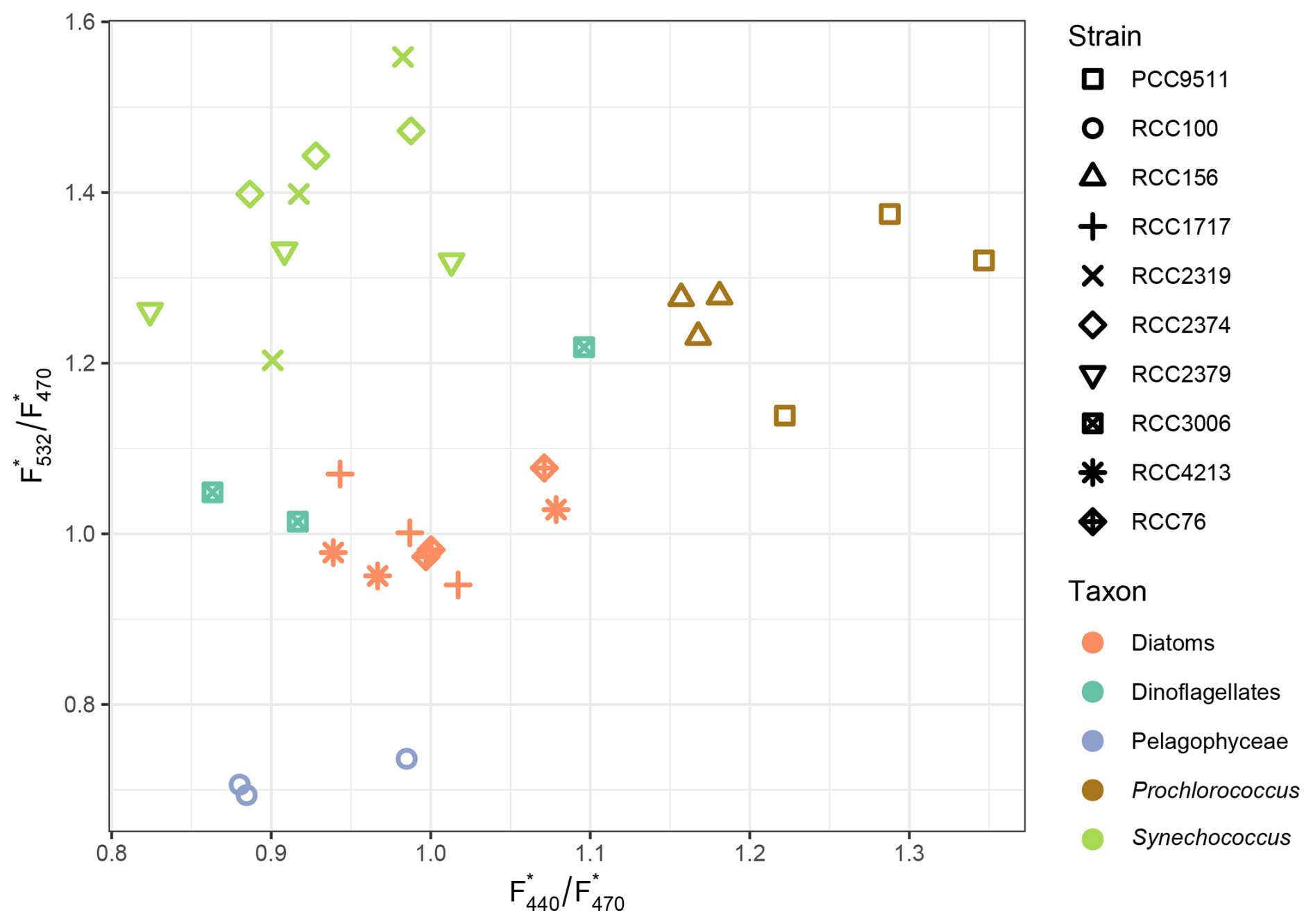
Figure 1 Scatterplot of F${{}^{\ast }}_{\mathrm{440}}$ $/$ F${{}^{\ast }}_{\mathrm{470}}$ vs. F${{}^{\ast }}_{\mathrm{532}}$ $/$ F${{}^{\ast }}_{\mathrm{470}}$ ratios for each phytoplankton strain grown in culture. The colour code indicates the taxon to which each strain belongs; the symbols indicate the strains, using the Roscoff Culture Collection code, when available (see Table 1).

The higher F${{}^{\ast }}_{\mathrm{532}}$ $/$ F${{}^{\ast }}_{\mathrm{470}}$ values observed for the Synechococcus taxon may be explained by their higher fluorescence at 532 nm, induced by the presence of phycoerythrin. Indeed, this phycobiliprotein is systematically found in open ocean Synechococcus and binds two chromophores, phycourobilin (λ_max ∼ 495 nm) and phycoerythrobilin (λ_max ∼ 545 nm), the latter thus being the most excited at 532 nm (Six et al., 2007; Grébert et al., 2018). It should be noted, however, that the phycoerythrobilin-to-phycourobilin ratio can vary in response to ambient light quality in some open-ocean Synechococcus strains through chromatic acclimation (Palenik, 2001; Humily et al., 2013), a capacity which may modulate the F₅₃₂ response of individual strains and introduce variability in the signal beyond what is captured by our laboratory measurements under fixed white light conditions. Consequently, the phycourobilin-rich strain RCC2379 expectedly exhibited a lower average F${{}^{\ast }}_{\mathrm{532}}$ $/$ F${{}^{\ast }}_{\mathrm{470}}$ ratio than the two other Synechococcus strains both being chromatic acclimaters which, in white light, exhibit a low phycourobilin to-phycoerythrobilin ratio (Palenik, 2001; Six et al., 2004; Humily et al., 2013). The fairly high F${{}^{\ast }}_{\mathrm{532}}$ $/$ F${{}^{\ast }}_{\mathrm{470}}$ ratio observed in Prochlorococcus strains are harder to explain, given their very low phycoerythrin content (Steglich et al. 2003, 2005). In contrast, the higher F${{}^{\ast }}_{\mathrm{440}}$ $/$ F${{}^{\ast }}_{\mathrm{470}}$ ratio of the HL-adapted PCC 9511 compared to the LL-adapted RCC156 may be explained by the much higher DV-Chla (λ_max ∼ 450 nm) to DV-Chlb (λ_max ∼ 475 nm) ratio of the former strain (Moore et al., 1995). The differences in fluorescence responses among diatoms, dinoflagellates, and Pelagophyceae are also likely related to their distinct content in accessory chlorophylls and carotenoids. In particular Fuco in diatoms and Pelagophyceae, and Peri in dinoflagellates, absorb light in the 440–532 nm range and transfer energy to Chl a via fluorescence resonance energy transfer, potentially contributing to the fluorescence signal measured at these excitation wavelengths (e.g., Bidigare et al., 1989; Bricaud et al., 2004; Ras et al., 2008; Meneghin et al., 2018). However, the efficiency of this energy transfer varies across taxa and physiological states, making the contributions of these carotenoids more challenging to interpret quantitatively than those of chlorophylls.

Our results are in line with numerous previous studies that demonstrated that pigment composition influences both light absorption and fluorescence emission spectra in phytoplankton, leading to taxon-specific fluorescence signatures (Yentsch and Menzel, 1963; Johnsen and Sakshaug, 2007; Hu et al., 2010; MacIntyre et al., 2010; Proctor and Roesler, 2010). More specifically, some laboratory studies using monospecific cultures demonstrated that fluorescence spectra vary significantly across taxa when multiple excitation and emission wavelengths are used (Yentsch and Menzel, 1963; Johnsen and Sakshaug, 2007; Poryvkina et al., 1994). More recent work has expanded on these findings by incorporating mixed communities, showing potential for determination of natural assemblages of phytoplankton (Hu et al., 2010; Escoffier et al., 2015). While Hu et al. (2010) included both monospecific and mixed cultures, as well as coastal marine samples, most of these studies were conducted under controlled laboratory conditions rather than in open-ocean environments.

Only a few studies have investigated fluorescence responses in natural, mixed phytoplankton communities (Seppälä and Balode, 1998; Hu et al, 2010; Proctor and Roesler, 2010; Thibodeau et al., 2014). Some of these studies benefited from conditions that enhanced pigment-specific fluorescence signals, such as reversed filtration to increase pigment concentration (Seppälä and Balode, 1998), high resolution of fluorescence excitation/emission spectra (Seppälä and Balode, 1998; Hu et al, 2010) or naturally high chlorophyll concentrations in bloom conditions (Proctor and Roesler, 2010). These conditions contrast sharply with those of the open ocean, where phytoplankton communities are more diverse, pigment concentrations are lower, and taxonomic differentiation based on MXF alone is more challenging.

Despite this complexity, our MXF measurements on mono-specific cultures are promising and coherent with Proctor and Roesler (2010), who further demonstrated that intra-taxon variance in specific fluorescence ratios was lower than inter-taxon variance. Both their study and the present one suggest that a multispectral MXF sensor with three excitation channels (440, 470, and 532 nm) can provide sufficient sensitivity to distinguish taxa in controlled conditions even though natural communities consist of mixed assemblages of taxa with complex pigment signatures, leading to less contrasted fluorescence response than for laboratory cultures. Therefore, in the following section, we investigate whether it is possible to resolve taxonomic composition from in situ phytoplankton fluorescence signals by analysing a year-long dataset from the NW Mediterranean Sea. Additionally, we assess whether combining MXF measurements with other bio-optical proxies could improve classification performance, in anticipation of future deployment of multispectral fluorometers on BGC-Argo profiling floats.

3.2 Phytoplankton communities in the NW Mediterranean Sea

Surface chlorophyll concentrations at the BOUSSOLE site can reach values up to 5 mg Chl a m⁻³ during the spring bloom and drop below 0.1 mg Chl a m⁻³ in summer, along with seasonal changes of the phytoplankton community composition (Marty et al., 2002; Antoine et al., 2020). In winter, pigment indicators of prymnesiophyte, namely 19^′-HF and 19^′-BF, are observed alongside Fuco, a marker of diatoms, and Allo, a marker of cryptophytes (Marty et al., 2002; Mayot et al., 2017). During the spring phytoplankton bloom, Fuco concentrations increase (Marty et al., 2002), which is likely related to an increase in diatoms. In summer, the mixed layer is phosphate-limited and phytoplankton communities are representative of stratified oligotrophic regions, with a prevalence of pigments specific to picophytoplankton, DV-Chla and Zea (Marty et al., 2008). This phytoplankton diversity is comparable to what is observed in temperate open-ocean regions (Vidussi et al., 2001; Marty et al., 2002; Lavigne et al., 2015; Mayot et al., 2017).

The composition of the phytoplankton communities in the field samples was analysed using a pigment-based clustering approach (see Sect. 2.4.2). The clustering allowed grouping samples with similar pigment composition and led to the discrimination of four distinct phytoplankton assemblages (clusters) over the year (Fig. 2a–d). All clusters are dominated by nanophytoplankton but vary significantly in the partitioning between micro- and picophytoplankton (Fig. 2e–h). The first cluster corresponds to winter communities as well as deep autumn communities, with a large proportion of picophytoplankton and a significant contribution of Chl b, a pigment typical of green microalgae, mostly flagellates (Bustillos-Guzmán et al., 1995). The second cluster coincides with the bloom community with a shared contribution of micro- and nanophytoplankton. This assemblage is characterised by a high Fuco contribution, typically associated with diatoms. The third cluster is associated with summer communities located at and below the level of the deep chlorophyll maximum and also exhibits a mixed composition of micro- and nanophytoplankton. Finally, the fourth cluster is characteristic of picophytoplankton communities in surface waters from summer to autumn, typically dominated by picocyanobacteria (Barlow et al., 1997).

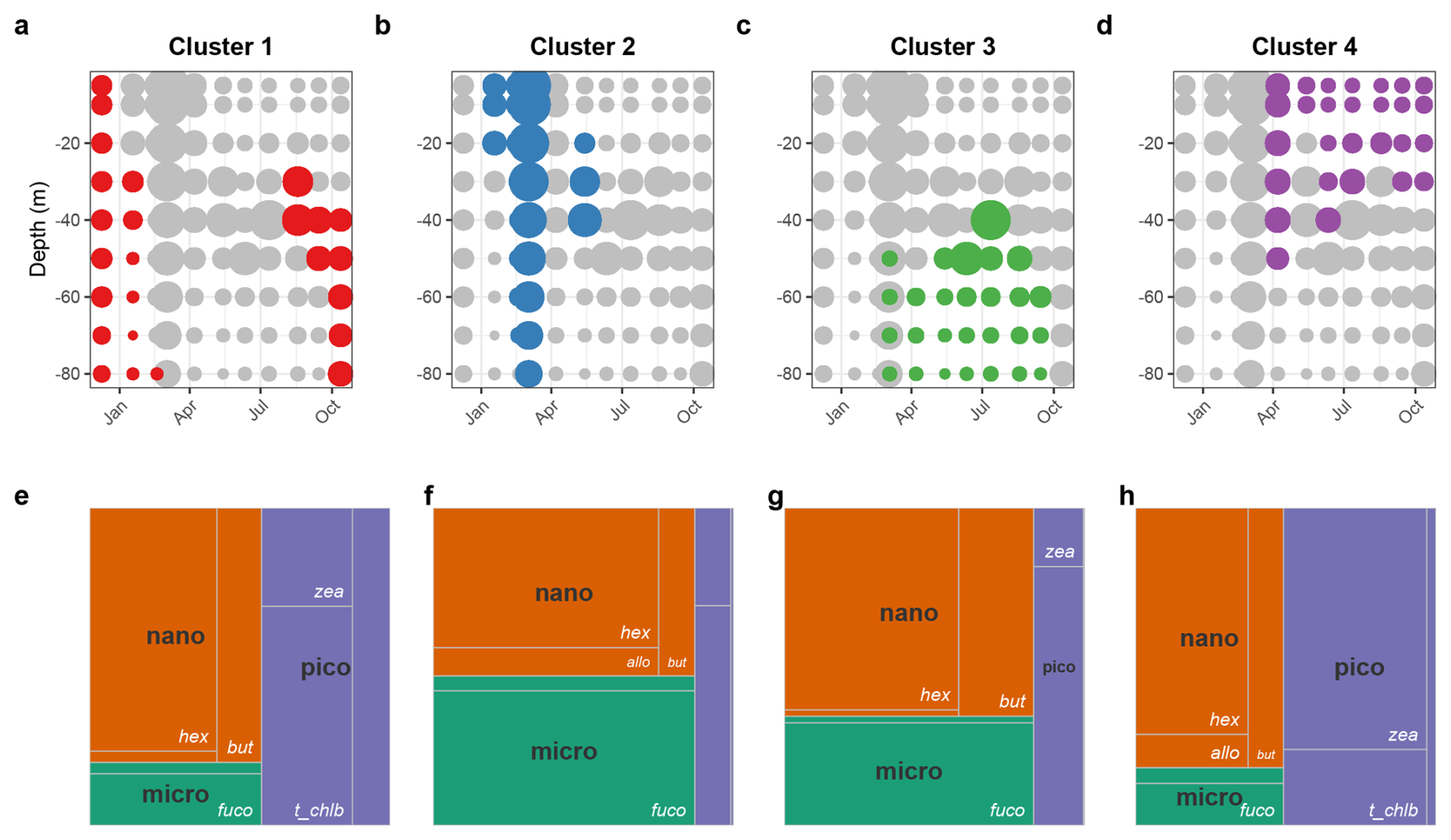
Figure 2 Distribution of the phytoplankton communities as determined from the cluster analysis applied to the field pigment data: (a–d) Vertical distribution of the four pigment-determined clusters indicative of the main phytoplankton communities encountered over an annual cycle in the NW Mediterranean Sea (BOUSSOLE site). The size of the dots indicates the Chl a concentration, used as a proxy of the phytoplankton biomass. (e–h) Tree map of the relative pigment concentration of each cluster (areas delimited by the grey lines), with the size class corresponding to the pigment taxa affiliation (colored).

The culture experiments demonstrated that phytoplankton taxa can exhibit distinct MXF fluorescence ratios under controlled conditions (Fig. 1). So, we compared the relative accessory pigment composition of the in situ clusters to that of the five laboratory characterised taxa. This analysis seeks to determine whether the field samples fall in the range of variability of accessory pigment composition of the culture samples.

Similar to the field samples, a CA (see Sect. 2.4.1) was applied to the pigment composition of the ten phytoplankton strains grown in the laboratory. This method allows a visualisation of the different strains in a space where the distance between two samples reflects their relative pigment composition similarity (Fig. 3). We observe three distinct groups corresponding to the different taxa represented by the ten selected strains. One is composed of diatoms and Pelagophyceae, while the two others correspond to Synechococcus and Prochlorococcus, respectively. This highlights a strong contrast in pigment composition between Synechococcus which has Zea, Prochlorococcus which has DV-Chla, DV-Chlb and Zea, and the nano- and microphytoplankton taxa that share many different pigments (Jeffrey et al., 1997; Veldhuis et al., 2005).

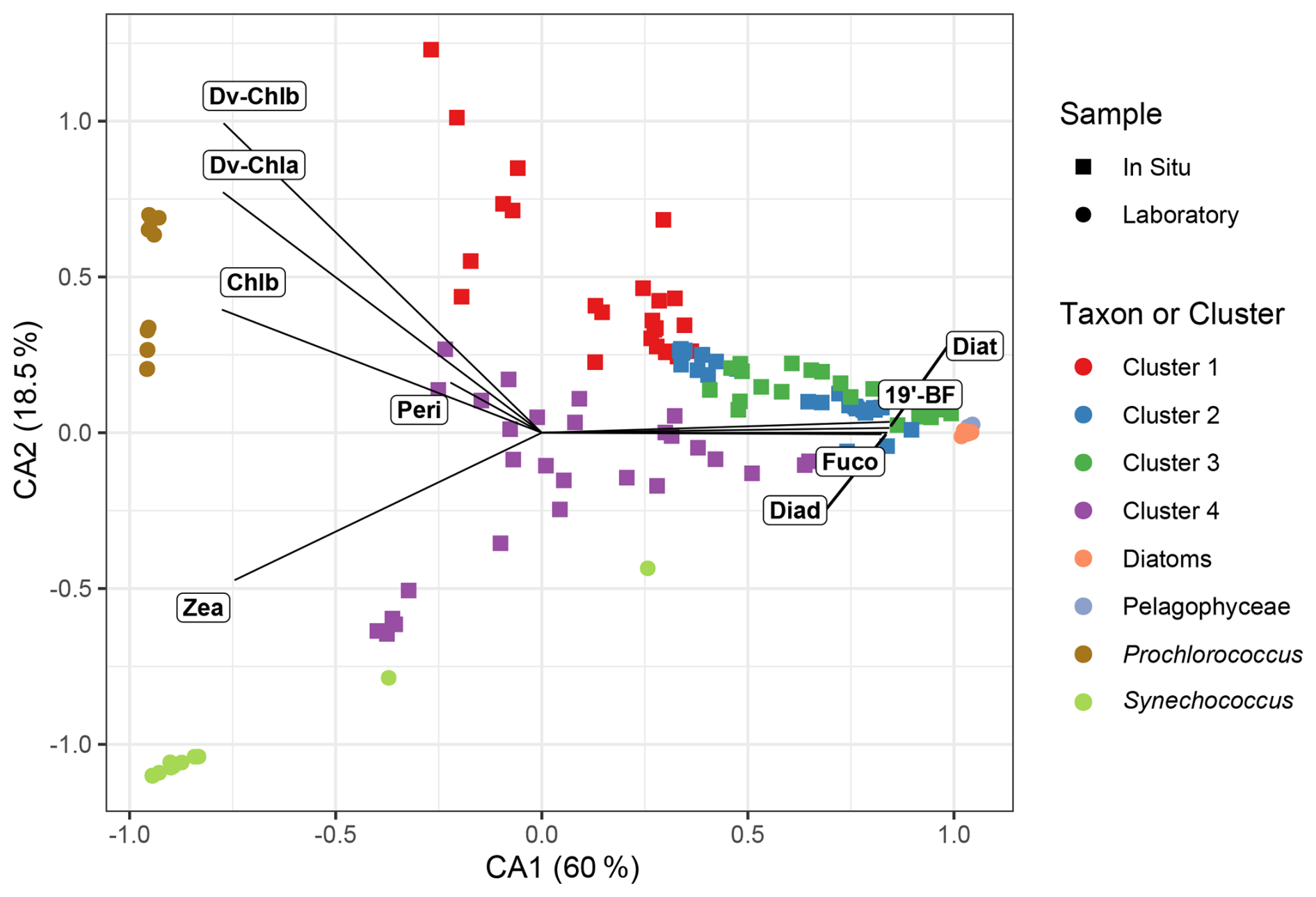
Figure 3 Correspondence analysis of the pigment concentrations of the strains grown in culture. The pigment concentrations measured in the NW Mediterranean (BOUSSOLE site) seawater samples are projected as supplementary observations and represented using the same colour code as in Fig. 2. 

The laboratory results provide a reference from which the projection space is computed, on which the field samples are projected (Fig. 3). The field data are evenly spread in the centre of the plan, indicating that the variability in the pigment composition of the field samples is similar to that observed in the laboratory cultures. Moreover, the four field-based clusters are fairly well distinguished in the CA, except for a few samples of cluster 1 with high CA2 values, due to the presence of 19^′-HF, a pigment absent from our reference strains. However, this pigment has a very similar absorption signature to other carotenoids like 19^′-BF or peridinin. We thus expect that the MXF sensor is sensitive enough to discriminate between different phytoplankton groups (clusters) characterised by distinct pigment composition in field samples.

In addition, we note that the in situ samples have lower eigenvalues (i.e., absolute values on CA axes) than the laboratory samples indicating that the pigment variability is less contrasted in the field than in laboratory samples. This is not surprising because of the complexity of the pigment composition in natural samples associated with mixed phytoplankton assemblages, instead of single taxa in monospecific cultures. This characteristic of open-ocean samples could somewhat hamper the possibilities of inferring information on phytoplankton community composition from MXF measurements, a hypothesis that is tested in the next section.

3.3 Discrimination of phytoplankton taxa from in situ MXF and additional bio-optical variables

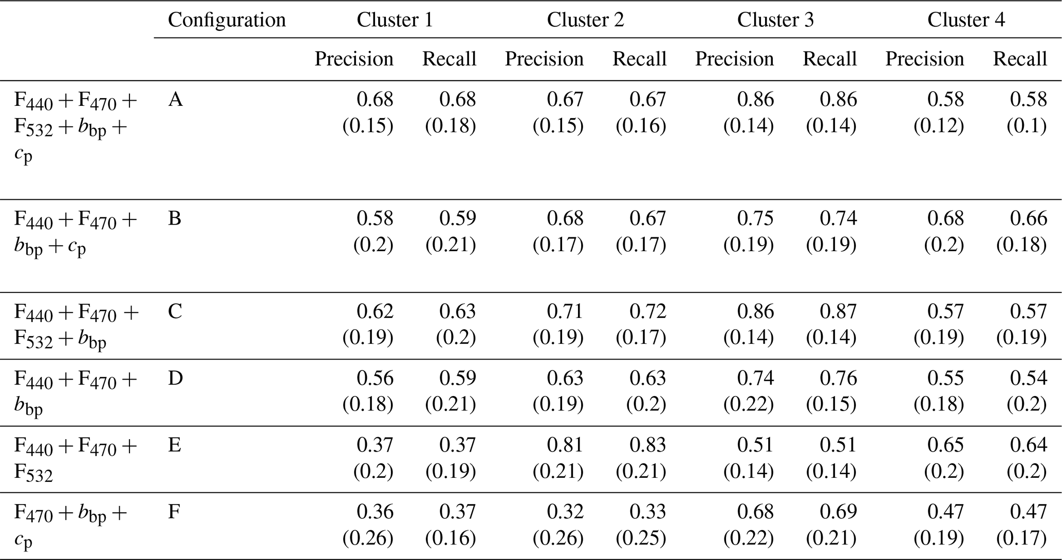
The predictive model (see Sect. 2.4.3) was tested using as inputs measurements from the MXF sensor alone (F₄₄₀, F₄₇₀, F₅₃₂), or in combination with measurements from a backscatterometer (F₄₄₀, F₄₇₀, F₅₃₂, b_bp) and a transmissometer (F₄₄₀, F₄₇₀, F₅₃₂, b_bp, c_p). Additionally, the model was also tested using measurements from a dual excitation channel fluorometer and backscatterometer (F₄₄₀, F₄₇₀, b_bp), or combined with a transmissometer (F₄₄₀, F₄₇₀, b_bp, c_p) (Fig. 4 and Table A1 in the Appendix). These two configurations are of particular interest as many BGC-Argo floats have been deployed with this specific set of sensors.

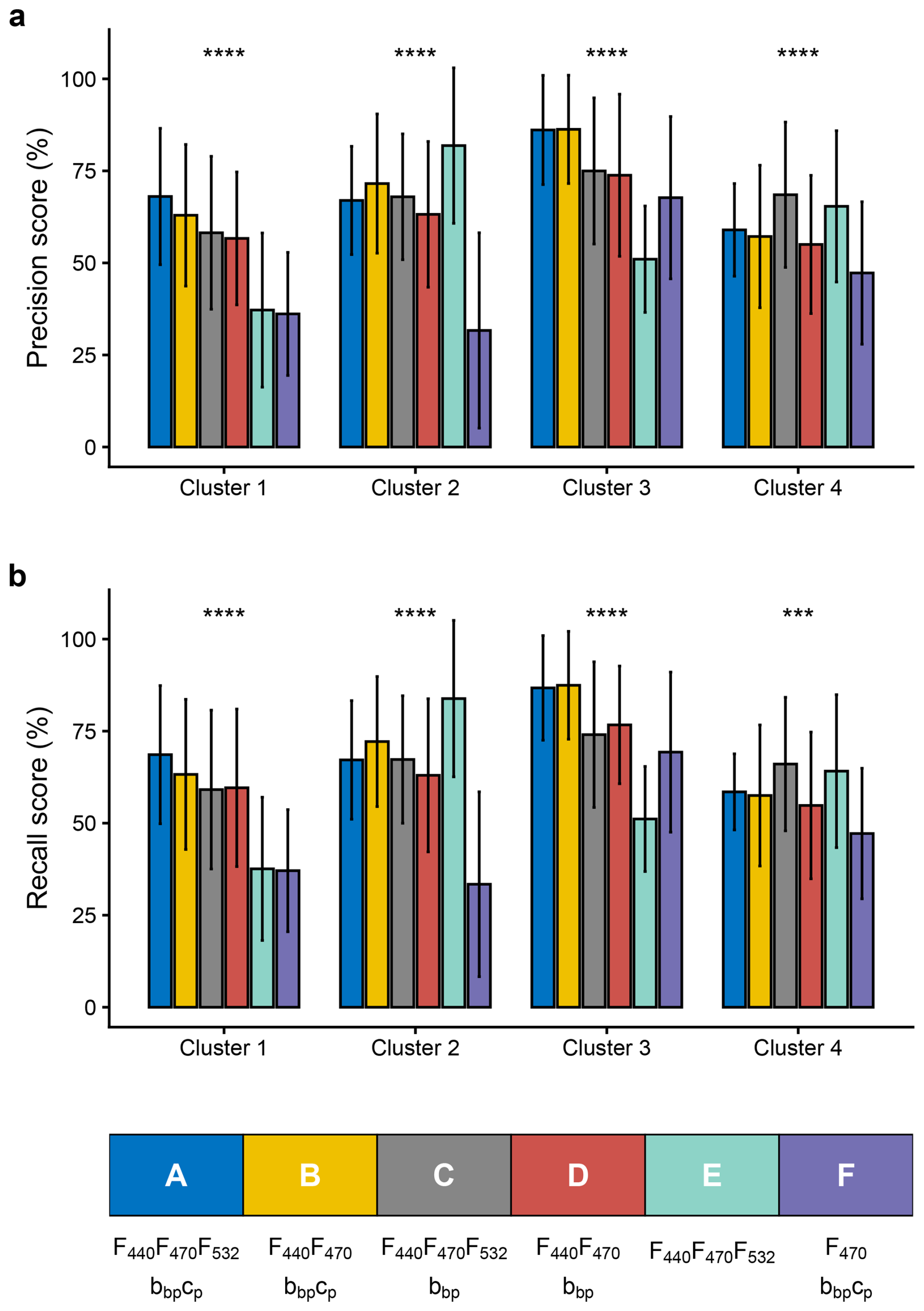
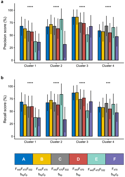
Figure 4 Precision and recall scores for phytoplankton community classification using different sensor package configurations. (a) Precision and (b) recall scores for predicting four phytoplankton clusters using various sensor combinations, either currently equipped on BGC-Argo profiling floats or suitable for future installations: full configuration (A: F₄₄₀, F₄₇₀, F₅₃₂, b_bp, c_p); dual channel fluorescence with backscatterometer and transmissometer (B: F₄₄₀, F₄₇₀, b_bp, c_p); MXF with b_bp (F₄₄₀, F₄₇₀, F₅₃₂, b_bp); dual channel fluorometer with backscatterometer (D: F₄₄₀, F₄₇₀, b_bp); MXF only (E: F₄₄₀, F₄₇₀, F₅₃₂) and single channel fluorescence with backscatterometer and transmissometer (F: F₄₇₀, b_bp, c_p). Precision represents the fraction of positive predictions that were correct, while recall indicates the fraction of true positives correctly identified. Error bars reflect variability across cross-validation runs. Within each cluster, differences among the six sensor configurations were assessed with a Kruskal–Wallis test, with significance indicated by stars (ns: p > 0.05; ^∗: p ≤ 0.05; ${}^{\ast \ast }$: p ≤ 0.01; ${}^{\ast \ast \ast }$: p ≤ 0.001; ${}^{\ast \ast \ast \ast }$: p ≤ 0.0001).

Considering the most comprehensive configuration, A (i.e., F₄₄₀, F₄₇₀, F₅₃₂, b_bp, c_p), the precision and recall scores of the HGB model are homogeneous among all four clusters with values between 60 % and 85 % (±15 %) (Fig. 4 and Table A1). These results based on annual sampling in the NW Mediterranean are quite robust, showing sufficient precision to demonstrate that MXF, when used in combination with a backscatterometer and a transmissometer, effectively allow four phytoplankton taxonomic groups to be distinguished. If we remove either the MXF sensor or the transmissometer, leading to measurements of F₄₄₀, F₄₇₀, b_bp and c_p, or F₄₄₀, F₄₇₀, F₅₃₂ and b_bp (i.e., configurations B and C, respectively), we observe similar precision and recall scores, and a marked variability between the clusters (Fig. 4 and Table A1). However, all four clusters displayed a mean precision of 67.25 % (±6.9 %) and 69 % (±12 %) for configurations B and C, respectively. When considering configuration D, which corresponds to a sensor load with a dual-channel fluorometer and a backscatterometer (i.e., F₄₄₀, F₄₇₀ and b_bp), the scores are significantly lower with a mean precision of 62 % (±8.7 %). The use of the MXF sensor only (configuration E, i.e. F₄₄₀, F₄₇₀and F₅₃₂) led to variable performances depending on the cluster. Thus, removing the transmissometer (c_p) or the 532 nm excitation fluorescence channel (F₅₃₂) seemingly induces a significant decrease in the general accuracy and recall scores of the model (Fig. 4). Finally, the configuration with only single-channel fluorescence measurements and two bio-optical indices (configuration F, i.e. F₄₇₀, b_bp, c_p) led to lower performance for every cluster, except for the picophytoplankton dominated one (i.e., cluster 4; see Fig. 2). This suggests that a configuration without MXF performs better when the phytoplankton communities have contrasted size structures.

Based on configuration A, which combines MXF and all bio-optical indicators, we can evaluate the predictive power of each descriptor. The mean importance of the descriptors in the discrimination of distinct phytoplankton clusters, as indicated by the impurity metrics (Fig. 5), highlights a significant role of all selected descriptors (b_bp $/$ c_p, F₄₄₀ $/$ F₄₇₀, F₄₄₀ $/$ c_p, F₅₃₂ $/$ F₄₇₀, F₅₃₂ $/$ b_bp, F₄₇₀ $/$ c_p, F₄₇₀ $/$ b_bp, F₄₄₀ $/$ b_bp), and particularly of b_bp $/$ c_p, F₄₄₀ $/$ F₄₇₀ and F₅₃₂ $/$ F₄₄₀ ratios. The high importance of the b_bp $/$ c_p ratio was expected as it has been already used as an indicator of the particle size distribution (Dall'Olmo et al., 2009; Slade and Boss, 2015; Organelli et al., 2020). Interestingly, the second and third strongest predictive descriptors correspond to the fluorescence ratios from the MXF sensor (F₄₄₀ $/$ F₄₇₀ and F₅₃₂ $/$ F₄₇₀). This indicates the strong added value of the MXF descriptors in the predictive model, in line with our laboratory results. These results also support the findings of both Proctor and Roesler (2010) and Thibodeau et al. (2014) who showed that the F₄₄₀ $/$ F₄₇₀ and F₅₃₂ $/$ F₄₇₀ fluorescence ratios are related to the taxonomic composition of phytoplankton communities. Finally, we note that the commonly used phytoplankton community index, F₄₇₀ $/$ b_bp ratio (Cetinić et al., 2015; Lacour et al., 2019; Terrats et al., 2020), has a notably lower predictive robustness in our analysis than all other ratios except F₄₄₀ $/$ b_bp. Therefore, the use of new sensor configurations, including a multiple excitation channel fluorometer and a beam attenuation transmissometer implemented on BGC-Argo floats, may have a stronger potential than previously described methods to detect seasonal succession of phytoplankton groups, with markedly different pigment composition or cell sizes (here picophytoplankton-dominated vs. microphytoplankton-dominated communities).

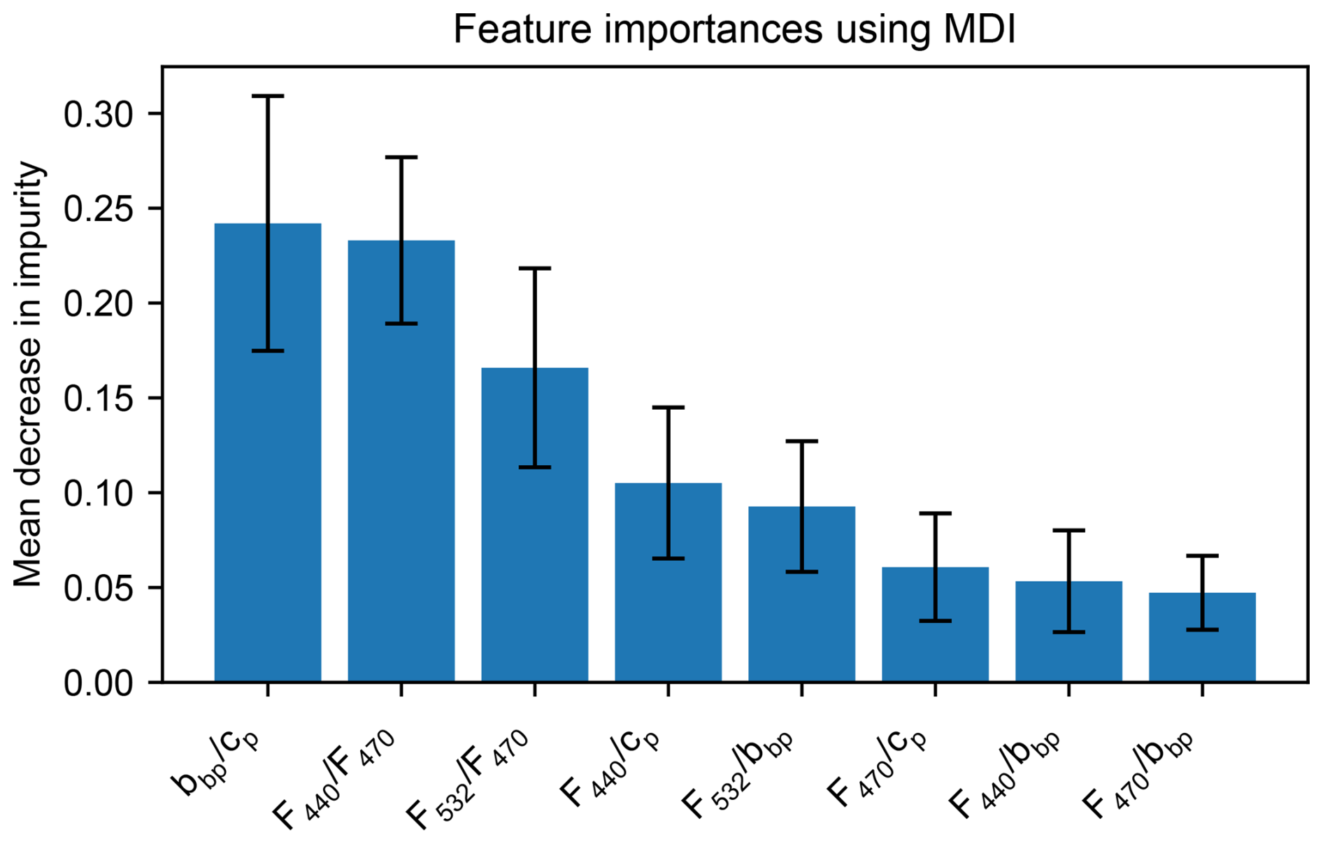
Figure 5 Importance of the different descriptors in the classification model, expressed as the mean decrease in impurity. The mean decrease in impurity reflects how much each descriptor contributes to improving the purity of the splits in the decision tree. A higher value indicates that the descriptor plays a more significant role in distinguishing (i.e., pigment-based clusters) in the model. Error bars indicate standard deviation of the mean decrease impurity across the 20 cross-validations.

3.4 Model tuning to predict phytoplankton communities

In the previous section, the classification model was evaluated for the prediction of four phytoplankton clusters representing the main communities observed over the annual cycle. Here, we further explore the sensitivity of the model to the predictive complexity by progressively reducing the number of clusters from four to three and two. This allows us to assess how model performance varies under simpler ecological scenari. First, we reduced the number of clusters from four to three by merging Clusters 2 and 3, the two clusters with the smallest distance, representing mixed nano- and microphytoplankton-dominated communities. The main distinction between these two clusters lies in their dominant pigments. Cluster 2 is indeed characterised by a higher relative contribution of Allo, while Cluster 3 is dominated by 19^′-HF. The three resulting clusters correspond to the surface summer picophytoplankton community associated with large concentrations of Zea (Cluster 4), the winter and deep summer picophytoplankton community with Chl b and DV-Chlb (Cluster 1), and the mixed micro- and nanophytoplankton community (Clusters 2 and 3 grouped together). Second, we reduced the initial number of four clusters to two, by merging Cluster 1 (dominated by Chl b-containing picophytoplankton) and Cluster 4 (dominated by Zea-containing picophytoplankton) to a picophytoplankton-dominated cluster, essentially grouping Synechococcus, Prochlorococcus and chlorophytes. The second cluster consists of the previously merged cluster (initially Clusters 2 and 3) composed of micro- and nanophytoplankton.

As presented in Sect. 3.3, we evaluated the classification model performances for different sensor configurations using the mean balanced recall metrics, which reflects the percentage of correctly classified samples. The same cross-validation method was applied to ensure consistency (Fig. 6). We first observed that a decrease in prediction complexity (specifically, a reduction in the number of clusters) does not consistently lead to an improvement in the classification model performance, and that the effect of such a reduction depends on the sensor configuration. When all sensors are included (configuration A), the model performs best in predicting 2 or 3 clusters than 4 clusters, achieving above 75 % recall. Similarly, the model using as inputs two fluorescence wavelengths, as well as the b_bp and c_p coefficients (i.e., configuration B) achieves above 75 % recall when predicting 2 or 3 clusters.

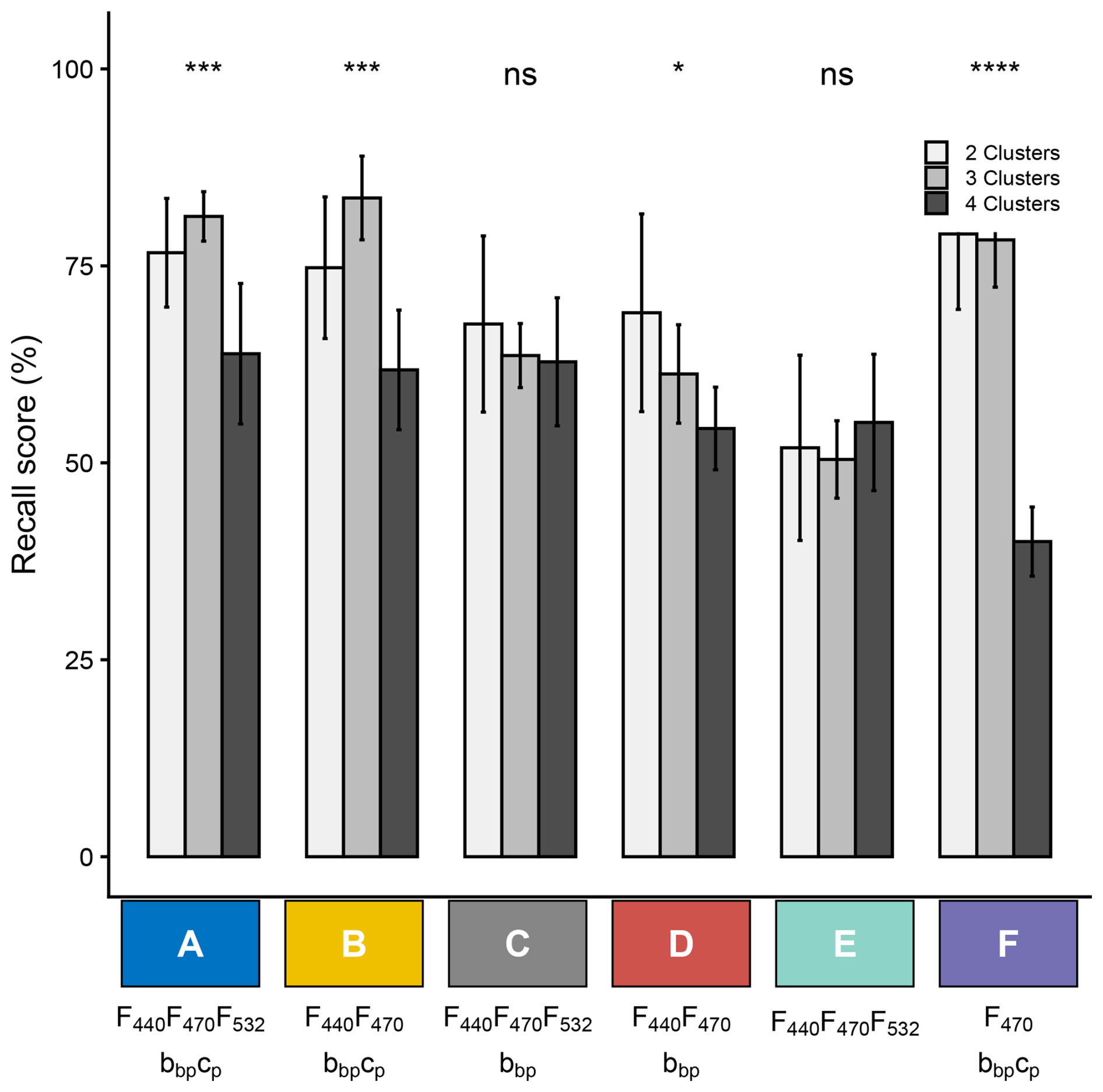
Figure 6 Values of the mean weighted recall resulting from cross-validation with different numbers of clusters and different sensor combinations, either currently equipped on BGC-Argo profiling floats or feasible for future deployments:  full configuration – A (F₄₄₀, F₄₇₀, F₅₃₂, b_bp, c_p); dual-channel fluorescence with backscatterometer and transmissometer - configuration B (F₄₄₀, F₄₇₀, b_bp, c_p); MXF with b_bp – configuration C (F₄₄₀, F₄₇₀, F₅₃₂, b_bp); dual-channel fluorometer with backscatterometer – configuration D (F₄₄₀, F₄₇₀, bbp); MXF only – configuration E (F₄₄₀, F₄₇₀, F₅₃₂); and single-channel fluorescence with backscatterometer and transmissometer – configuration F (F₄₇₀, b_bp, c_p). Error bars reflect variability across cross-validation runs. Within each configuration, differences among the six cluster configurations were assessed with a Kruskal–Wallis test, with significance indicated by stars (ns: p > 0.05; ^∗: p ≤ 0.05; ${}^{\ast \ast }$: p ≤ 0.01; ${}^{\ast \ast \ast }$: p ≤ 0.001; ${}^{\ast \ast \ast \ast }$: p ≤ 0.0001).

It is worth noting that the model using as inputs bio-optical measurements from sensors already implemented on some BGC-Argo floats (i.e, configuration F with single-channel fluorescence, b_bp and c_p) demonstrates strong predictive capabilities for 2 or 3 clusters, achieving recall values of 72 % and 74 %, respectively. In the two-cluster prediction scenario, one cluster predominantly comprises picophytoplankton, such as Synechococcus and Prochlorococcus, while the other includes a mix of nano- and microphytoplankton. Interestingly, previous studies have shown that the combination of F₄₇₀, b_bp, and c_p effectively correlate with phytoplankton community size structure (Veldhuis et al., 2005; Brewin et al., 2011; Cetinić et al., 2015; Sauzède et al., 2015; Rembauville et al., 2017; Terrats et al., 2023) supporting our findings. In the three-cluster scenario, the model must distinguish between two different types of picophytoplankton communities rather than one. These communities exhibit markedly different photoacclimation profiles, with deep-water communities displaying a F₄₇₀ $/$ b_bp ratio significantly distinct from that of surface communities (Bellacicco et al., 2016; Graff et al., 2016). Thus, the model successfully discriminates phytoplankton communities according to their average size and photoacclimation status. However, when the nano- and microphytoplankton-dominated cluster is further divided into two distinct communities based on varying carotenoid composition, the model performance declines markedly, resulting in a recall score of only 40 %. This low score, compared to the high predictive performance of the other models, that all include multiple fluorescence with at least two wavelengths (i.e., configurations A to E), highlights the importance of MXF for pigment-based remote classification of phytoplankton communities.

When using MXF data only (i.e., configuration E), the model recall performance drops to approximately 50 %, whatever the number of predicted clusters. In comparison, models with the MXF sensor and a transmissometer (i.e., configuration C) reach around 65 % recall, regardless of the number of clusters to be predicted. Adding the particulate backscattering coefficient (b_bp, configuration A) slightly increases the recall score to around 75 % when predicting 2 or 3 clusters. This highlights the importance of incorporating additional bio-optical indices with MXF, such as b_bp and c_p, to enhance the phytoplankton group classification model. Furthermore, when the backscatterometer and transmissometer are present, the MXF 532 nm fluorescence channel does not improve the model performance (configuration A and B). This indicates that, overall, when bio-optical sensors measuring b_bp and c_p can be used as inputs, only two fluorescence wavelengths are needed to achieve an optimal classification of phytoplankton communities.

These findings demonstrate that meaningful phytoplankton taxonomic information can be retrieved from MXF signals. If the standard BGC-Argo configuration (i.e., configuration F) with one single-channel fluorescence and two optical indices (b_bp and c_p) shows good prediction performances for predicting two and three clusters, adding one more fluorescence wavelength (i.e., configurations A to E) significantly improves the performance when predicting four clusters. Thus, our results demonstrate that MXF is a promising avenue for remote classification of phytoplankton community composition.

Our results also highlight that the predictive skill of individual descriptors, particularly the 532 nm fluorescence channel, depends on both the way clusters are defined and the ecological context in which communities occur. When clusters retain a strong contribution of Chl b-containing taxa (e.g., chlorophytes) or phycoerythrin-rich picocyanobacteria (Synechococcus), the F₅₃₂ $/$ F₄₇₀ ratio provides valuable information on community composition. However, when such groups are merged into broader assemblages, the influence of F₅₃₂ diminishes and the model relies more heavily on size- or biomass-sensitive proxies such as c_p and b_bp. Ecologically, this reflects the fact that pigment-based contrasts are strongest when communities differ in accessory pigment composition, while size-structure proxies dominate when communities are merged across pigment gradients. From a broader perspective, this sensitivity also explains why the usefulness of F₅₃₂ will vary geographically: in regions where Synechococcus or green flagellates are recurrent and occasionally abundant (e.g., coastal upwelling systems), the inclusion of a 532 nm excitation channel may improve the discrimination of these specific groups by enhancing the excitation of accessory pigments that are less efficiently excited at shorter wavelengths, as discussed in previous studies (Morel, 1997; Saito et al., 2005). In contrast, in persistently oligotrophic waters such as the subtropical gyres, where the picophytoplankton pool is largely dominated by Prochlorococcus, the added value of F₅₃₂ may be reduced, although this hypothesis remains to be tested with dedicated multi-region datasets.

More broadly, our results allow us to draw a general framework linking sensor configuration to achievable phytoplankton classification performance in the context of BGC-Argo observations. The level of community discrimination that can realistically be achieved depends on two interacting factors: the ecological contrast between the communities to be distinguished (e.g., differences in pigmentation, size, or photoacclimation status), and the spectral and optical information available from the sensor suite. When communities differ primarily in size structure, such as pico- versus microphytoplankton dominance, bio-optical proxies alone (i.e., b_bp and c_p) provide sufficient discriminatory power, while the MXF contributes only limited additional value. In this regime, the standard BGC-Argo configuration (configuration F) already achieves recall scores above 70 %. MXF becomes essential when communities share similar size structures but differ in pigment composition, for instance, when distinguishing between nano- and microphytoplankton assemblages characterised by contrasting carotenoid signatures, or between distinct picophytoplankton communities dominated by Prochlorococcus vs. Synechococcus. In these cases, adding even a single fluorescence channel (440 or 470 nm) to the standard configuration provides a statistically significant improvement in classification performance. The 532 nm channel provides additional value specifically in environments where phycoerythrin-rich taxa such as Synechococcus or Chl b-containing organisms are recurrent and abundant, but its contribution diminishes when such groups are absent or merged into broader assemblages. In terms of minimum sensor requirements, our results suggest that combining two fluorescence channels (440 and 47 nm) with b_bp and c_p represents an optimal and achievable configuration for BGC-Argo platforms. This configuration achieves over 75 % recall in scenarios distinguishing (1) two phytoplankton clusters (i.e. picophytoplankton vs mixed nano- plus microphytoplankton assemblages) or (2) three clusters (i.e. a mixed nano- plus microphytoplankton, a Synechococcus-like and a Prochlorococcus-like assemblages). This configuration corresponds to dual-channel fluorometers already implemented on part of the BGC-Argo fleet, suggesting that meaningful phytoplankton community information could be extracted from existing deployments without requiring new instrumentation. Adding a third fluorescence channel at 532 nm provides incremental benefit specifically for pigment-based discrimination at finer taxonomic resolution, and would be the recommended configuration for regions or seasons where Synechococcus or green flagellates are ecologically important.

4 Conclusion and perspectives

Monitoring phytoplankton community composition is essential for understanding marine biogeochemical cycles, particularly those related to oceanic carbon dynamics. However, this remains challenging in open-ocean environments due to the limitations of current autonomous sensor technologies and the complex bio-optical signature of mixed phytoplankton assemblages. This study specifically evaluated whether multispectral fluorescence (MXF), using three excitation channels (440, 470, and 532 nm), alone or in combination with other bio-optical measurements readily available on BGC-Argo platforms, can provide meaningful taxonomic discrimination of phytoplankton assemblages. We used a gradient boosting model, chosen for its high performance and good explainability, to assess the potential of MXF for autonomous, in situ monitoring of phytoplankton community structure. We assessed the model's performance across different sensor configurations, reflecting realistic BGC-Argo float payloads, and across varying levels of classification complexity (i.e., number of predicted pigment-based clusters). While lab conditions confirmed MXF sensitivity across five groups, field predictions required combining MXF with bio-optical indices to extract meaningful information from complex, mixed phytoplankton assemblages. Sensor configurations already implemented on BGC-Argo, such as single-wavelength fluorescence with b_bp and c_p, performed well for simple phytoplankton communities (two or three clusters, i.e. strong size contrast between predicted assemblages). However, MXF becomes essential when communities share similar size distributions but differ in pigment composition, such as when distinguishing nano- from microphytoplankton assemblages or contrasting picophytoplankton communities. In these cases, combining two fluorescence channels (440 and 470 nm) with b_bp and c_p represents an optimal and realistic configuration, achieving over 75 % recall across multiple community scenarios and corresponding to dual-channel fluorometers already deployed on part of the BGC-Argo fleet.

Overall, our results suggest that integrating MXF into BGC-Argo platforms could significantly enhance our ability to monitor shifts in phytoplankton communities, particularly among groups with overlapping size distributions. This advancement would provide valuable insights into ecosystem dynamics and the role of phytoplankton taxonomic composition across broad spatial and temporal scales, enabled by the autonomous sampling capabilities of BGC-Argo floats, in open-ocean biogeochemical cycles.

Future work should aim to generalise these findings across diverse oceanic regions and refine the predictive model to account for a broader variety of phytoplankton taxa. Building a standardised dataset linking phytoplankton community composition, from pico- to micro-size classes, to MXF and bio-optical measurements will be crucial for improving our understanding of phytoplankton dynamics through autonomous observations.

Appendix A

Table A1 Mean and standard deviation of precision and recall scores from the cross validation (repeated prediction of clusters from the machine learning model using randomly picked samples for training and testing). The standard deviation is indicated in parentheses. Each line corresponds to a specific combination of sensors, either currently deployed on BGC-Argo profiling floats or suitable for future deployments:  full configuration (A: F₄₄₀, F₄₇₀, F₅₃₂, b_bp, c_p); dual channel fluorescence with backscatterometer and transmissometer (B: F₄₄₀, F₄₇₀, b_bp, c_p); MXF with backscatterometer (C: F₄₄₀, F₄₇₀, F₅₃₂, b_bp); dual channel fluorometer with backscatterometer (D: F₄₄₀, F₄₇₀, b_bp); MXF only (E: F₄₄₀, F₄₇₀, F₅₃₂) and single channel fluorescence with backscatterometer and transmissometer (F: F₄₇₀, b_bp, c_p).