Modelling the impacts of marine heatwaves on plankton in the Salish Sea

Marine heatwaves are discrete events of prolonged anomalously warm ocean temperatures caused by a combination of atmospheric forcing and ocean processes. The Northeast Pacific Marine Heatwave (NEP-MHW) was first detected in the Salish Sea in 2014 and persisted in the region until 2017. Here, we used a three-dimensional coupled biophysical model, SalishSeaCast, to examine the impacts of the NEP-MHW on the physics and the plankton in the Salish Sea. Sixteen years (2007–2022) of model results were used to follow the trajectory of the NEP-MHW into key regions of the Salish Sea. Model results were compared to observation data collected over the same period. We resolved the specific impacts of the NEP-MHW versus the impacts of warming via other large-scale climate indices operating on longer time scales. Model results showed that the strongest physical signatures of the NEP-MHW were evident in the Juan de Fuca region wherein warming was favourable for the growth of both diatoms and nanoflagellates. In comparison, the direct warming from the NEP-MHW impacted the Strait of Georgia (SoG) to a lesser degree but warm water anomalies persisted in this region until the end of our study period in 2022. Both temperature and nitrate in the upper layer of the SoG were strongly linked to the North Pacific Gyre Oscillation and diatom biomass decreased during this prolonged warming period. Our results highlight the need to recognize that multiple types of marine heatwaves associated with different large-scale climate indices can occur simultaneously, even within a single waterbody such as the Salish Sea, each with distinct impacts on the local food web.

1 Introduction

Marine heatwaves (MHWs) are discrete events of prolonged (i.e., longer than 5 d) and anomalously warm ocean temperatures in a given region (Pearce et al., 2011; Hobday et al., 2016) often caused by a combination of atmospheric forcing and/or ocean processes (Oliver et al., 2021). Large-scale climate patterns have been shown to influence the likelihood that a MHW event will occur (Scannell et al., 2016; Holbrook et al., 2019). For example, the El Niño Southern Oscillation (ENSO) is the dominant mode of interannual climate variability worldwide and the leading cause of MHW occurrences (Oliver et al., 2018). Globally, MHW events have increased in frequency and duration (Oliver et al., 2018) and are expected to further increase as a result of long-term ocean warming (Frölicher et al., 2018).

The Northeast Pacific Marine Heatwave (NEP-MHW), initially called “The Blob” (Bond et al., 2015), developed in the Gulf of Alaska during the boreal winter of 2013 and was the largest MHW on record in the region (Di Lorenzo and Mantua, 2016). The development of the NEP-MHW was attributed to strong positive anomalies in sea level pressure, which reduced winds and ultimately suppressed the heat flux from the ocean to the atmosphere (Bond et al., 2015). Later, the cause of this MHW was attributed to ocean heat transport, as opposed to anomalous air-sea heat fluxes into the ocean (Oliver et al., 2021), and thus linked to tropical-extratropical teleconnections (Bond et al., 2015; Di Lorenzo and Mantua, 2016; Oliver et al., 2021). More recently, Chen et al. (2023) showed that warm air temperatures played the most significant role in the development of the NEP-MHW. Although there is no clear consensus on how the NEP-MHW was formed, the North Pacific Gyre Oscillation (NPGO) and the Pacific Decadal Oscillation (PDO) were shown to reflect temperature and sea level pressure changes during this time period (Di Lorenzo and Mantua, 2016). Overall, the likelihood of a MHW occurring in the NE Pacific is elevated by about 17 % during years that are in a positive PDO phase, yet ENSO and NPGO are also known to play significant roles in the occurrences of MHW in this region (Holbrook et al., 2019).

The NEP-MHW had widespread ecosystem impacts in the North Pacific. For example, lower chlorophyll a concentration (a proxy for phytoplankton biomass) and a shift to a higher relative abundance of picoplankton as a result of temperature-induced changes to biological processes were observed near Ocean Station Papa (Yang et al., 2018). Similarly, high sea surface temperature (SST) anomalies, fresher nearshore water, and anomalous periods of downwelling were associated with a decrease in chlorophyll a in the Southern California Current System (Zaba and Rudnick, 2016). With respect to zooplankton, the copepod community off of the coast of Oregon shifted to smaller, lipid-poor taxa, which decreased the quality of food available to higher trophic levels (Peterson et al., 2017). Similarly, the abundance of the smaller copepod Calanus pacificus, which is typically most abundant off the coasts of California and southern Oregon, increased throughout the Northeast Pacific (Fisher et al., 2020). The NEP-MHW also significantly impacted many commercially important shellfish and finfish fisheries because of a widespread coastal toxic bloom of the diatom Pseudo-nitzschia (McCabe et al., 2016). A mass mortality event of common murres (Uria aalge) as well as other fish, bird, and mammal species was observed throughout the region from 2014–2017 (Piatt et al., 2020).

The Salish Sea is a large coastal waterbody in the southwest portion of British Columbia, Canada, and northwest portion of Washington, USA. The strongest reported impacts of the NEP-MHW within the Salish Sea appeared in autumn 2014 and persisted through the 2015–2016 El Niño wherein anomalous water column warming was observed (Chandler et al., 2017; Khangaonkar et al., 2021). Khangaonkar et al. (2021) used a modelled simulation of the NEP-MHW period and found a small decrease in both phytoplankton and zooplankton biomass relative to reference conditions in the Salish Sea. Observed zooplankton biomass was anomalously high in all regions within the U.S. waters of the Salish Sea during 2015, remaining high until 2017 in Admiralty Inlet and Central Basin (Winans et al., 2023). Biomass of some of the dominant zooplankton taxa (e.g., copepods, euphausiids, and gelatinous groups) showed variable and basin-specific responses during NEP-MHW years, but these patterns may have been related more to local drivers rather than due to warming from NEP-MHW (Winans et al., 2023). In contrast, zooplankton biomass was below average in 2014 in the Strait of Georgia (Canadian waters; Perry et al., 2021). Further, the increased water temperatures during the NEP-MHW in Haro Strait were associated with decreased body condition of age-0 Pacific sand lance (Ammodytes personatus), an important forage species for piscivorous seabirds (Robinson et al., 2023).

Here, we used a three-dimensional coupled biophysical model, SalishSeaCast, to examine the impacts of the NEP-MHW on the physics and the plankton in the Salish Sea. Sixteen years (2007–2022) of model results were used to follow the trajectory of the NEP-MHW into key regions of the Salish Sea to determine the extent to which this event impacted lower trophic level dynamics. Given that other warming phenomena (e.g., negative phase of the NPGO and El Niño events) were co-occurring over the study period, we aimed to resolve the specific impacts of the NEP-MHW versus the impacts associated with other large-scale climate indices often operating on longer time scales in the region. Temperature and nitrate were analyzed over the full water column as well as averaged over the relevant depth layers associated with estuarine circulation in the Salish Sea to track incoming water. In order to examine the cascading effects of warming throughout the food web, we then focused our analysis on two main regions: (i) the Juan de Fuca (JdF) region, which is directly connected to the Pacific Ocean, and (ii) the Central Strait of Georgia (SoG), which is a deep, semi-enclosed basin within the Salish Sea. The JdF region is generally well-mixed to depths of 50+ m, and has strong flow exchange meaning low residence time (Ianson et al., 2016). Phytoplankton in this region are light-limited and temperature controlled (Mackas and Harrison, 1997). Diatoms dominate throughout the year and productivity follows the light cycle rather than having a clear spring bloom, resulting in high depth-integrated productivity during the summer (Jarníková et al., 2022). In comparison, the Central SoG is well-stratified, particularly through the summer due to high river flows and being semi-enclosed (Suchy et al., 2023). Residence times are longer in the SoG and surface temperatures are high in the summer (Ianson et al., 2016). Phytoplankton in the Central SoG are light-limited in the spring, but nutrient-limited in the summer, leading to a classic spring bloom followed by a nanoflagellate-dominated summer (Jarníková et al., 2022, Nemcek et al., 2023). Phytoplankton and zooplankton were then examined over the upper water column of these two regions. Model results were ground-truthed with observation data collected over the same period. Results from this study were interpreted and discussed in the context of the multiple warming phenomena operating during the same time in the Salish Sea. Since MHWs are projected to increase in frequency, there is a need to understand their complex impacts on marine ecosystems.

2 Methods

2.1 Study Site

The Salish Sea is a waterbody comprised of four major areas: the Strait of Georgia (SoG), Puget Sound (PS), Haro Strait, and Juan de Fuca Strait (JdF) which connects the region to open ocean waters (Fig. 1). The main source of freshwater into the region is the Fraser River, resulting in an estuarine-like circulation with surface waters leaving the SoG via the JdF (Pawlowicz et al., 2007). The roughly 100 km long JdF simultaneously brings in estuarine inflow waters at depth (100–200 m) carrying offshore waters which are high in nutrients and low in oxygen (Pawlowicz et al., 2007). Average flushing time, a measurement of water exchange (typically one third of the residence time), in the SoG is 125 d compared to 47 d in PS (MacCready et al., 2021). Water entering the SoG at depth during estuarine exchange is comprised of a combination of the intermediate water being brought into the JdF and surface SoG water that has been mixed extensively in the Haro Strait region (Ianson et al., 2016). During the summer months, 70 % of the water entering the Salish Sea via the JdF comes from north and offshore Pacific sources (Beutel and Allen, 2024). However, in winter a combination of southern shelf water and, to a lesser extent, Columbia River plume water, makes up over 80 % of the inflow (Beutel and Allen, 2024). Our study focused on five main regions of interest: JdF, Haro Strait, Central Basin in Puget Sound, Central SoG, and Northern SoG (Fig. 1) in order to follow the trajectory of the NEP-MHW of 2014–2017 and its potential impacts on plankton in the Salish Sea.

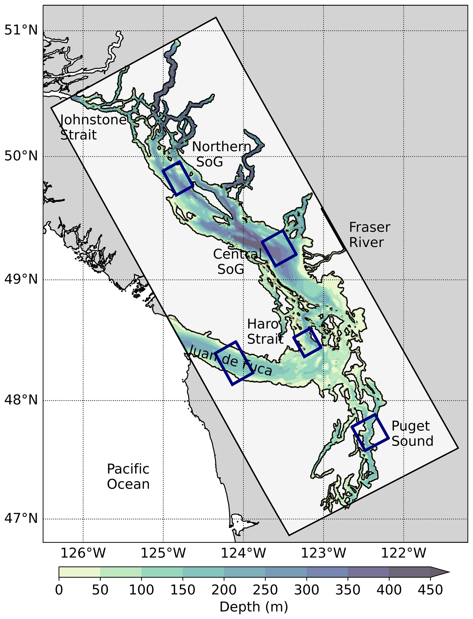
Figure 1 Map of the Salish Sea study area. Model domain is indicated with the light grey box. Selected sub-regions for analysis are shown in blue boxes. Bathymetry is overlain to highlight regional differences.

2.2 Study Period

Our modelled study period was from 2007 to 2022 (Fig. 2). The NEP-MHW formed during winter 2013 into 2014 (Bond et al., 2015) and persisted through to 2017, yet several other warming signals were present during this same period. In this paper we consider two additional large-scale climate signals: the North Pacific Gyre Oscillation (NPGO), which fluctuates on approximately decadal timescales, and the Southern Oscillation Index (SOI) operating on shorter (2–7 years) time scales. Negative values of both NPGO and SOI have previously been associated with positive SST anomalies (Masson and Cummins, 2007), coupled with high Fraser River discharge and weak winds in the SoG (Suchy et al., 2019). Hereafter, negative values of NPGO (post-2013) will be referred to as warm-phase NPGO years and sustained negative SOI values will be referred to as El Niño events. Further, strong relationships have been shown between the NPGO and SOI and plankton dynamics within the Salish Sea (Li et al., 2013; Suchy et al., 2022, 2025a). The NPGO represents the second empirical orthogonal function (EOF) of monthly residual SST anomalies in the North Pacific (Di Lorenzo et al., 2008). The SOI is calculated as pressure differences between the tropical eastern and western Pacific, providing a traditional measure of El Niño and La Niña events in the Pacific Ocean (Wallace et al., 1998). Monthly NPGO Index data were downloaded from (http://www.o3d.org/npgo/npgo.php, last access: 1 December 2025) and monthly SOI Index data were downloaded from (https://www.bom.gov.au/climate/enso/soi/, last access: 2 July 2026). In addition, a resurgence of positive SST anomalies referred to as the Blob 2.0 appeared in the summer of 2019 in the Northeast Pacific (Amaya et al., 2020). Our results for the NEP-MHW of 2014 to 2017 are considered within the context of these other climate signals which were also operating over the modelled period.

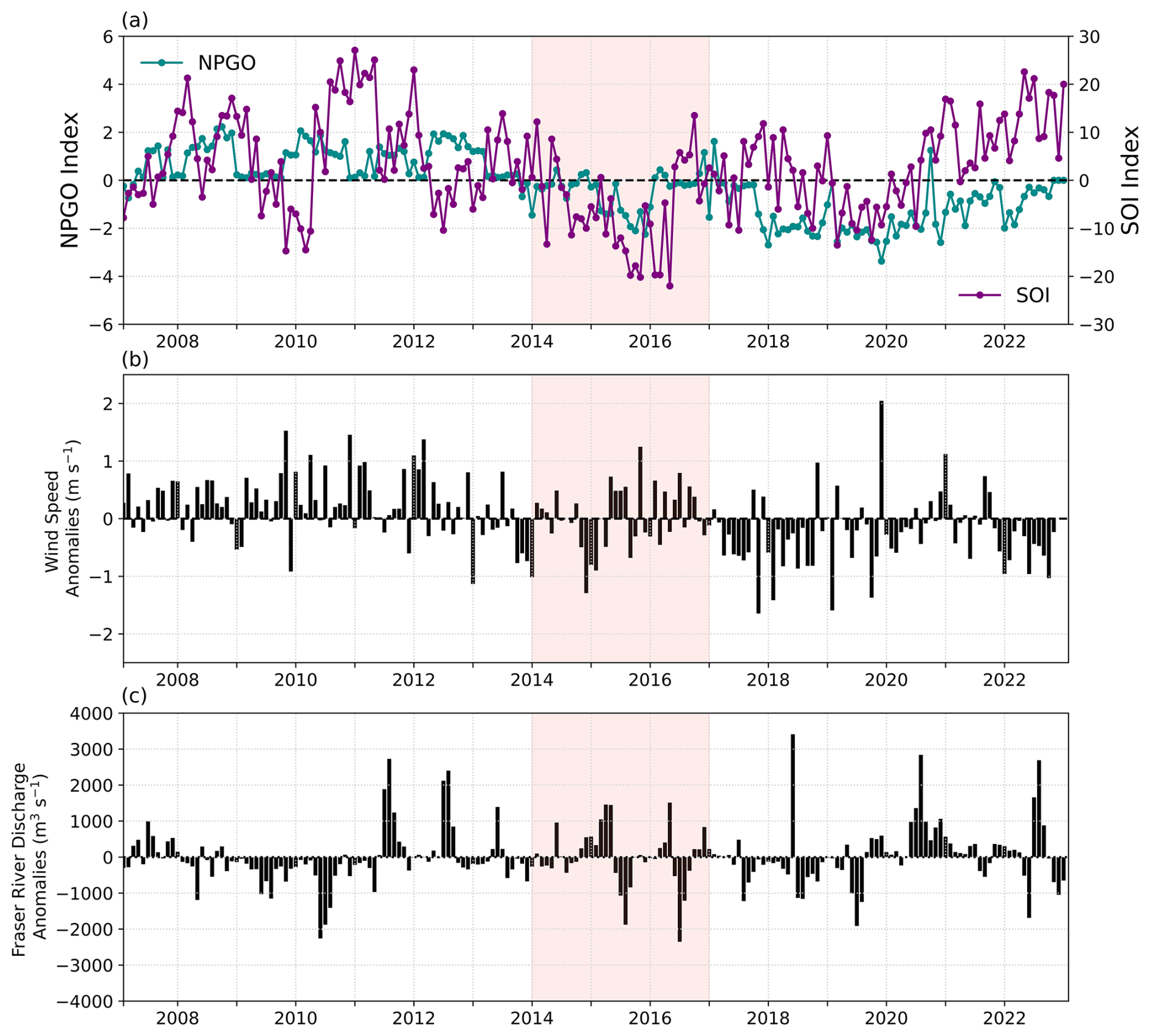
Figure 2 (a) Monthly North Pacific Gyre Oscillation (NPGO) index and Southern Oscillation Index (SOI) values during the modelled study period of 2007 to 2022, (b) monthly wind speed anomalies calculated over the Central Strait of Georgia, and (c) monthly anomalies in Fraser River Discharge. The NEP-MHW of 2014–2017 is indicated with pink shading.

2.3 SalishSeaCast Model

The SalishSeaCast model domain covers the entire Salish Sea (Fig. 1) with a horizontal resolution of approximately 500 m and a vertical resolution ranging from 1 at the surface to 27 m at 400 m depth. The physical component of SalishSeaCast is an implementation of Nucleus for European Modelling of the Ocean (NEMO Version 3.6; Madec et al., 2017) and is described in detail in Soontiens et al. (2016) and Soontiens and Allen (2017) with subsequent relevant changes outlined in Olson et al. (2020); Jarníková et al. (2022); and Stang and Allen (2025). Comprehensive evaluations of SalishSeaCast model have already been completed for nitrate (Olson et al., 2020), chlorophyll a (Olson et al., 2020; Jarníková et al., 2022), and zooplankton (Suchy et al., 2023). This study was based on v202111 of SalishSeaCast. The initial conditions for v202111 are from the previous model version v201905 (Jarníková et al., 2022). The model was spun up for five years prior to the first model year of 2007 to allow variables to reach equilibrium.

The model uses real-time data from Environment and Climate Change Canada (ECCC) as input for the Fraser River discharge (Soontiens and Allen, 2017) in addition to daily river flows for over 150 other rivers in the region (Stang and Allen, 2025). Atmospheric forcing (winds, solar radiation) is derived from High Resolution Deterministic Prediction System (HRDPS) atmospheric model output (Milbrandt et al., 2016). SalishSeaCast has two open boundaries for temperature, salinity, and nutrients: a northern boundary at Johnstone Strait and a western boundary at the mouth of Juan de Fuca Strait. Prior to 2013, western boundary conditions were based on fields from NEP 3.6 (Lu et al., 2017). After 2013, open boundary conditions were based on fields from the LiveOcean model (Davis et al., 2014; Siedlecki et al., 2015). Northern boundary conditions are based on temperature and salinity climatologies (Dosser et al., 2021).

The biological component of the model, SMELT (Salish Sea Model Ecosystem-Lower Trophic), follows the transfer of the model's currency (nitrogen) between nutrients, primary producers, grazers, and detrital pools with coupled silicon and oxygen cycling (Olson et al., 2020). The nutrients in the model are nitrate, ammonium, and silicon. Differences between v202111 and the previous model version (v201905; Jarníková et al., 2022) are provided in the Supplement (Tables S1–S9). The ciliate group (M. rubrum) was removed due to its consistently low contribution to overall phytoplankton biomass and the lack of improvement in model performance when previously included. Therefore, two groups of primary producers are present in the current version of the model: diatoms and nanoflagellates. Functional light dependence was switched to a potential energy curve with constants chosen to match the old response closely. The sinking calculation for biological tracers switched from upstream to incorporation in the Total Variation Diminishing (TVD) advection. Lastly, the nitrogen to oxygen coupling for various processes was updated and a parameter for sediment oxygen demand, proportional to the amount of organic matter sinking out of the model domain, was added to effectively allow an oxygen flux into the sediments uncoupled to outgoing nitrate flux. Dissolved silica was set to a concentration of 120 µm Si in Puget Sound rivers based on data provided by the Washington Department of Ecology and was kept at 59.57 µm Si in all other rivers (Olson et al., 2020).

Diatoms in the model have the highest maximum growth rates, the highest optimal light requirements, and are the only class to take up silicon (Olson et al., 2020). Nanoflagellates have the lowest maximum growth rate but compete better at low nitrogen concentrations and high temperatures (Olson et al., 2020; Jarníková et al., 2022). A previous evaluation of the model phytoplankton classes against high performance liquid chromatography (HPLC) data from the Canadian waters of the Salish Sea (Nemcek et al., 2023) showed that larger, centric diatoms are well represented by the model diatom class, whereas the model nanoflagellate class showed the strongest relationships with cryptophytes, prasinophytes, and haptophytes (Suchy et al., 2025a).

The temperature response for each phytoplankton group is set so that the optimal temperature for growth for diatoms (12 °C) and nanoflagellates (18 °C) match those of diatoms and dinoflagellates in Khangaonkar et al. (2012), after model experiments with these settings showed improved summer chlorophyll bias. Diatoms become nitrate-limited at a half-saturation constant of 2.0 µM N, whereas the half-saturation constant prescribed for nanoflagellates is 0.1 µm N. Additionally, the model includes biogenic silica, detrital particulate organic nitrogen (PON), and dissolved organic nitrogen (DON). Phytoplankton growth in the model may be limited by temperature, light, or nutrients (nitrate/ammonium, silicon).

Heterotrophs in SalishSeaCast are represented by two zooplankton classes: zooplankton class 1 (Z1) and zooplankton class 2 (Z2). Identification of which zooplankton taxa are represented by Z1 or Z2 was determined by evaluations against observation data (Suchy et al., 2023). The Z1 class freely evolves based on model dynamics (Olson et al., 2020) and represents taxa with traits such as relatively small body size, short life cycles, or high grazing rates, and whose growth rates respond quickly to local conditions (e.g., non-overwintering copepods, copepod nauplii, larvaceans; Suchy et al., 2023). Z2 are the highest trophic level whose grazing impact is included in the model and represents taxa with larger body size, longer life cycles, and slower grazing rates (e.g., overwintering copepods, euphausiids, amphipods; Suchy et al., 2023). The domain-mean Z2 biomass is constrained due to a seasonal climatology imposed as part of the model closure (see Suchy et al., 2023).

Given the strong constraint of Z2 as the model's closure term, Z2 biomass may respond differently compared to Z1 within the model framework. The Z2 biomass is distributed spatially throughout the model domain in proportion to food availability. Thus, spatial variability in the distribution of Z2 throughout the domain will directly reflect differences in the spatial distribution of Z2 prey items. Both Z1 and Z2 feed on diatoms, nanoflagellates, Z1, and PON, with each zooplankton class having different prey preferences set in the model. Z1 has the highest grazing preference for nanoflagellates (30 %), followed by diatoms (26 %), whereas Z2 has the highest preference for diatoms and Z1 (29 % each). However, the actual proportion of grazing depends on both preference and the relative abundance of each prey item. Olson et al. (2020) provides a full description of the biological model for version 201812 of SalishSeaCast. Subsequent changes, including those affecting zooplankton rates, were made for v201905 (Jarníková et al., 2022; Suchy et al., 2023). Adjustments made to the biology for the current version of the model (v202111) are provided in Tables S2–S4.

2.4 Model Data

We analyzed 16 years (2007–2022) of monthly model output from SalishSeaCast. Model data were averaged across each of the five study regions (blue boxes in Fig. 1). All model data are presented as monthly anomalies, which were calculated by subtracting the climatological mean (i.e., the mean for each month averaged over all 16 years) from the value for each month within a given year. Excluding the NEP-MHW years (2014–2017) in the mean did not significantly change the anomalies. Model output for Conservative Temperature (Θ; hereafter referred to as temperature in °C) and nitrate (mmol N m⁻³) are shown with time versus depth plots, as well as being averaged over specific depth ranges (0–50, 50–150, 150 m to bottom). Model results are discussed primarily for the surface (0–50 m) as this depth layer is most relevant to both phytoplankton and zooplankton. A depth range of 0–50 m was chosen in order to balance where we know the phytoplankton are growing (i.e., the euphotic zone) and where we know the model Z1 and Z2 are concentrated. For our two regions of focus, JdF and Central SoG, zooplankton in the SalishSeaCast model are concentrated mainly in the upper 50 m of the water column (see Suchy et al., 2023). Furthermore, previous studies in the region commonly define the surface layer as the 0–50 m depth layer in order to clearly delineate between this layer and the underlying intermediate waters (e.g., Pawlowicz et al., 2007; Ianson et al., 2016). When comparing model output against observations, however, depth layers are defined by the available observational data and are described for each comparison accordingly in Sect. 2.5. Information for deeper layers is provided in the Supplement. Halocline strength, a proxy for water column stratification, was calculated as the difference in salinity divided by the difference in depth of the two model grid cells wherein the maximum salinity gradient was observed and provides an indication of how much energy is required to mix the water column. Hourly wind data from HRDPS were interpolated onto the model grid and then calculated as mean monthly wind speed values for the Central SoG region only. Daily Fraser River discharge data from 2007–2022 were obtained from Environment and Climate Change Canada (https://wateroffice.ec.gc.ca/search/historical_e.html, last access: 2 July 2026) from Station 08MF005 at Hope, BC, and then used to calculate monthly anomalies. Model output for phytoplankton (diatoms and nanoflagellates) and zooplankton (Z1 and Z2) biomass were depth-averaged over the 0–50 m depth range to capture the full extent of the euphotic zone across regions (mmol N m⁻³). In addition, we calculated the extent to which temperature dependence and nitrate limitation was limiting to phytoplankton growth based on phototrophic growth rate equations and parameters set in the model. Detailed equations, first described in Olson et al. (2020) and Suchy et al. (2025a) but modified for v202111 are provided in the Supplement. Climatologies (2007–2022) for nitrate limitation coefficients and temperature dependence were calculated. Limitation coefficients range from 0 to 1, with higher values reflecting more nitrate limitation on growth. In contrast, higher values for temperature dependence mean that temperatures were more favourable for growth. Time series data are presented as monthly anomalies to highlight seasonal and interannual variability. Positive anomalies indicate less limitation/temperature dependence on growth, whereas negative anomalies mean growth was more limited/temperature dependent compared to the climatology. We focus our discussion on diatoms, which is the most variable prey item for Z1 and Z2 in the model. Limitation plots for nanoflagellates, which are less limited by nitrate and temperature compared to diatoms, are provided in the Supplement. Pearson Product-Moment Correlations were used to analyze the relationships between temperature and nitrate anomalies versus the NPGO and SOI in the JdF and Central SoG regions.

2.5 Observation Data

Nitrate, chlorophyll a (Chl a), and zooplankton data were obtained from numerous sources to compare our model results with observations in the JdF and Central SoG regions. Nitrate and Chl a data were initially compiled by Parker MacCready (University of Washington; https://github.com/parkermac/LO/tree/main/obs, last access: 1 December 2025). Zooplankton observation data were provided by the Institute of Ocean Sciences, Fisheries and Oceans Canada, and are described in detail for the model evaluations presented in Suchy et al. (2023). The zooplankton data used in this study can be downloaded from (https://data.cioospacific.ca, last access: 1 December 2025). Model and observation data were averaged over the same approximate regions. To maximize the number of model-observation comparisons, nitrate and Chl a were averaged over the 0–10 and 0–50 m depth ranges, respectively, whereas zooplankton were averaged over the full water column for both model and observations. Mean annual values for nitrate, Chl a, and zooplankton were then calculated over pre-MHW (2007–2013), MHW (2014–2019 to capture the NEP-MHW and the Blob 2.0), and post-MHW (2020–2022) years for comparison with model data across the same time periods. Model units (mmol N m⁻³) were converted to biomass units using a Chl : N ratio of 2 for phytoplankton (mg m⁻³) and a C : N ratio of 4.9 for zooplankton (mg C m⁻³; see Suchy et al., 2023). One-way ANOVA was used to test for statistically significant differences between pre-MHW, MHW, and post-MHW years. F-statistics (F) and p-values are reported with a significance threshold of α=0.05. If the one-way ANOVA detected significant differences, post hoc Tukey Honestly Significant Difference (HSD) tests were performed to identify which of the three groups of means were significantly different.

3 Results

3.1 Physical Drivers

3.1.1 Temperature

Overall, the strongest positive temperature anomalies occurred during two time periods across all regions: during the 2009–2010 El Niño event and during the NEP-MHW years; however, regional variability in the strength of these anomalies was evident (Figs. 3, 4). Positive temperature anomalies of up to 1.0 °C were observed in the 0–50 m (surface) depth layer in JdF from the end of 2009 through to the end of 2010 (El Niño event; Figs. 3a, 4a). The 2010 El Niño event was also evident in the SoG with positive temperature anomalies occurring mid-2009 and throughout 2010 in the Central and Northern SoG. Unlike the JdF region, positive anomalies in the 0–50 m layer in the SoG were periodically interrupted with intrusions of cooler water at the end of 2009 (Fig. 4). A period of negative temperature anomalies then followed the 2010 El Niño event in all regions, persisting until the end of 2013 (Fig. 4).

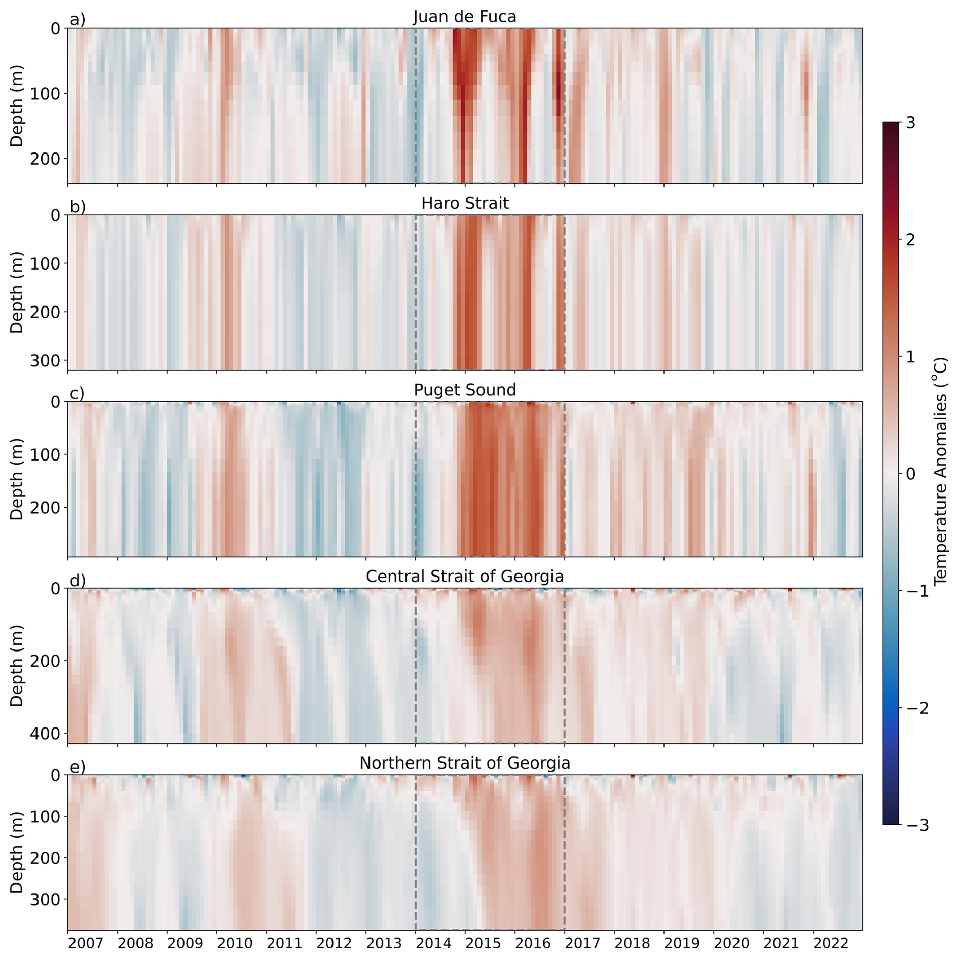
Figure 3 Model-based temperature anomalies versus depth in the different sub-regions of the Salish Sea from 2007 to 2022. Red indicates positive temperature anomalies and blue represents negative temperature anomalies. The NEP-MHW of 2014–2017 is outlined with dashed grey lines. Note that the vertical (depth) scales vary, reflecting the maximum depth of each region.

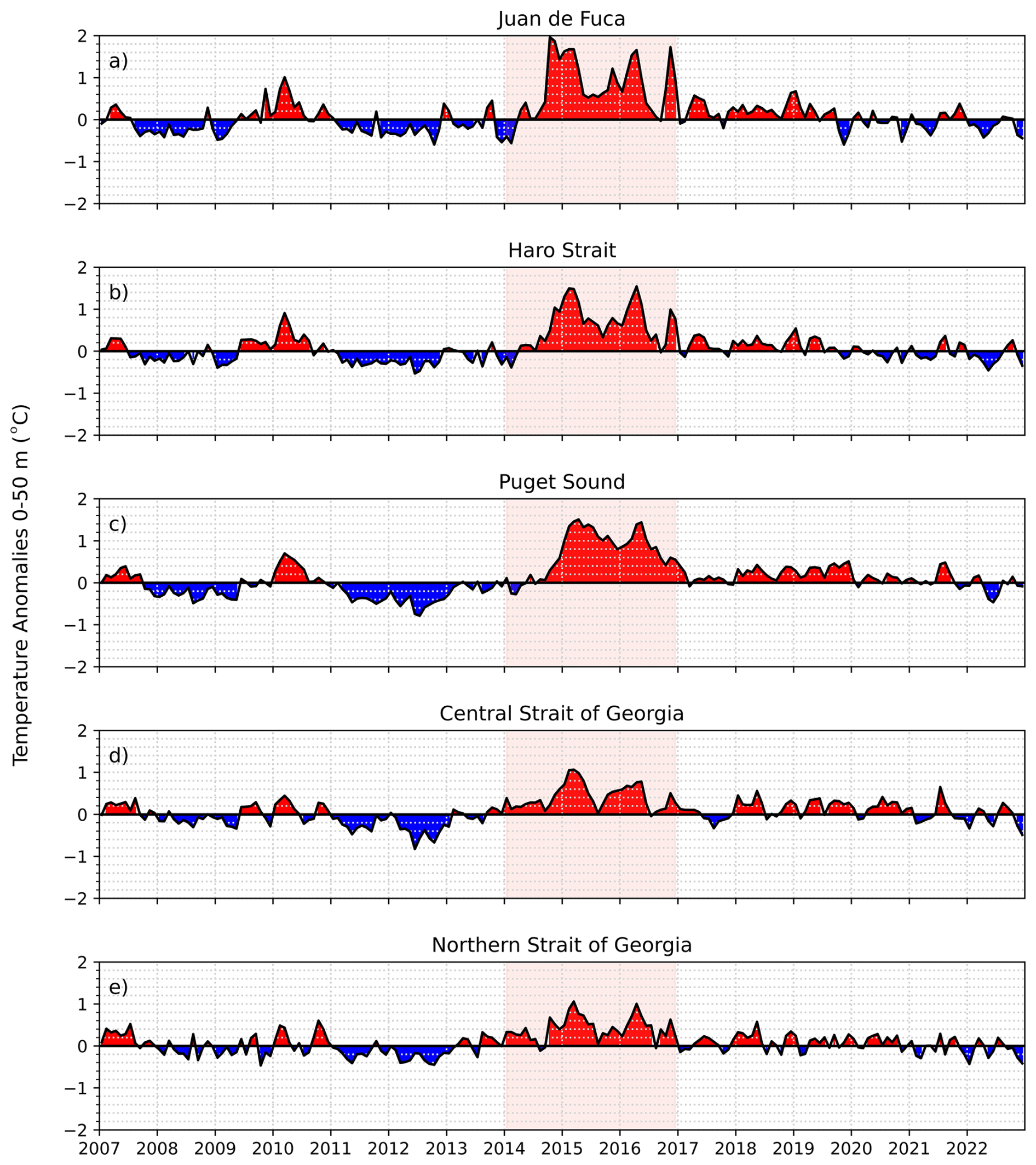
Figure 4 Mean model-based 0–50 m temperature anomalies in the different sub-regions of the Salish Sea from 2007 to 2022. Temperature anomalies for the 50–150 and 150 m to bottom depth ranges are provided in the Supplement(Figs. S1–S2).

Strong positive temperature anomalies appeared in the surface waters of the JdF region in mid-2014, reaching 2.0 °C above the mean by the end of the year and persisting through 2017, consistent with the NEP-MHW years (Figs. 3a, 4a). After mid-2019, negative temperature anomalies in the JdF region returned until the end of our time series in 2022. Temperature anomalies in the 50–100 m (intermediate) and 150 m to bottom (deep) depth layers were similar to those observed for the upper water column except that the warm anomalies in these layers arrived in pulses during the winter months from 2014–2017, and then again in the winter of 2019 (Figs. S1, S2). Temperature anomalies in Haro Strait and Puget Sound were similar to those observed in JdF at all depth layers; however, the surface (0–50 m) layer reached maxima of 1.5 °C above the mean in Haro Strait and Puget Sound, respectively, suggesting this region exhibited slightly less warming compared to JdF (Figs. 3, 4, S1–S2).

Positive temperature anomalies in the 0–50 m depth layer reached maximum values of 1.1 °C in early 2015 in the Central and Northern SoG, respectively, which were the lowest warming anomalies out of any of our study regions during NEP-MHW years (Fig. 4). Most notably, the Central SoG remained warm until the end of 2022, indicating a longer-term warming signal that cannot be explained solely by the NEP-MHW.

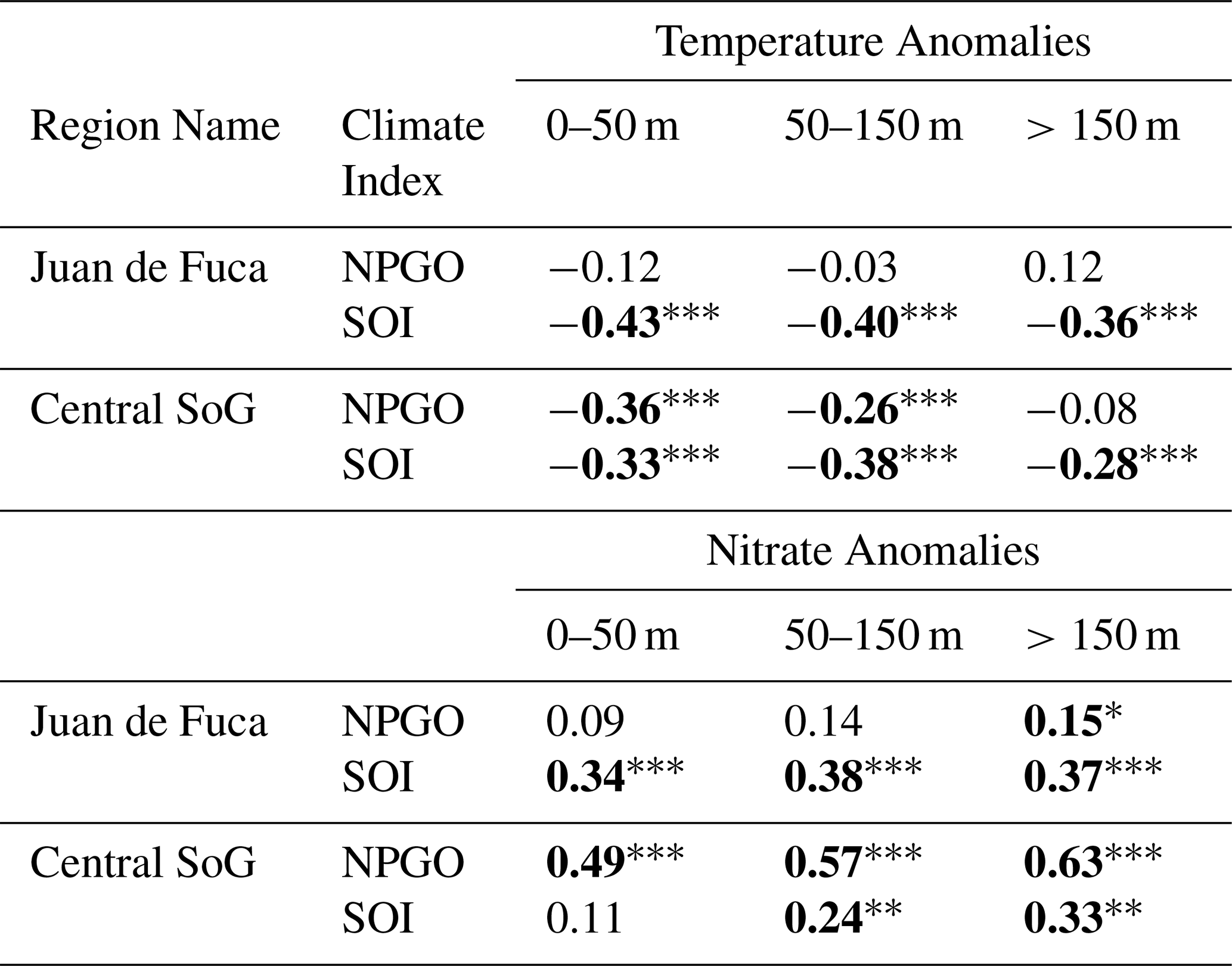
Significant relationships were found between surface temperature anomalies in the Central SoG and the NPGO ($r=-\mathrm{0.36}$, p<0.001) and between surface temperature anomalies and the SOI ($r=-\mathrm{0.33}$, p<0.001). In contrast, surface temperature anomalies in the JdF region were significantly correlated to the SOI ($r=-\mathrm{0.43}$, p<0.001), but not to the NPGO ($r=-\mathrm{0.12}$, p=0.09; Table 1).

Table 1 Pearson Product-Moment Correlations used to assess the relationship between temperature and nitrate anomalies versus large-scale climate indices (North Pacific Gyre Oscillation; NPGO and Southern Oscillation Index; SOI) for the Juan de Fuca and Central Strait of Georgia regions. Statistically significant relationships are indicated in bold with the following annotations: ${}^{*}=p<\mathrm{0.05}$, ${}^{**}=p<\mathrm{0.01}$, ${}^{***}=p<\mathrm{0.001}$.

We note here that the intermediate (50–150 m) and deep (>150 m) layers in the Central and Northern SoG showed extended warming after both the 2010 El Niño and the 2015 El Niño/NEP-MHW (Figs. S1–S2). Positive temperature anomalies were evident in these depth layers until early 2011, followed by a cooler period until the end of 2014. After the arrival of the NEP-MHW in 2014, these layers stayed warm until 2020 when negative temperature anomalies returned until the end of 2022.

3.1.2 Halocline Strength

The Central SoG and PS regions had the strongest haloclines (i.e., more stratification) whereas haloclines in the JdF and Haro Strait regions were weak (almost constantly mixed; Fig. 5). From 2007–2014 halocline strength periodically showed positive anomalies during spring and summer months in the Central SoG (Fig. 5d), which corresponded to periods of low winds in the Central SoG region and high Fraser River discharge (Fig. 2b, c). Negative anomalies in halocline strength during this time corresponded to negative anomalies in Fraser River discharge and positive wind anomalies in the Central SoG (Fig. 2b, c). Although negative halocline anomalies occurred throughout 2019 in Puget Sound, (Fig. 4c) strong stratification signals persisted in the Central SoG until the end of 2022 (Fig. 5d) most likely a result of the weak winds that were prevalent from 2013 until the end of our study period (Fig. 2b).

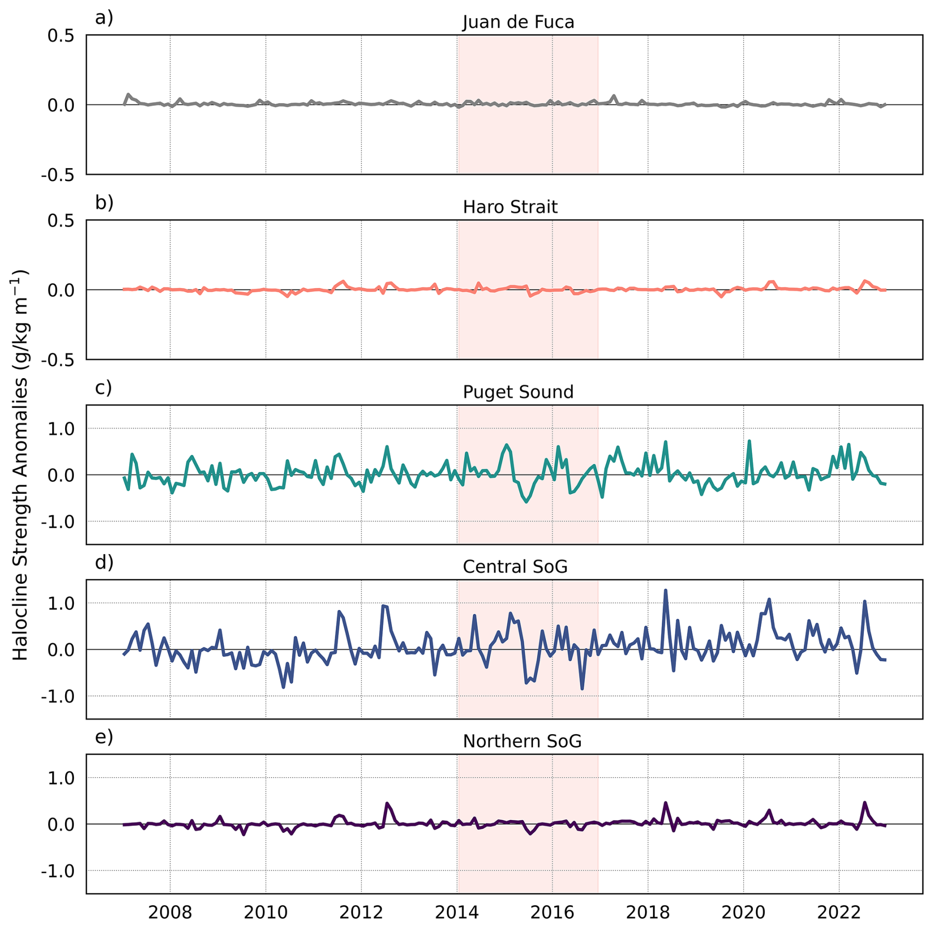
Figure 5 Anomalies in mean model-based halocline strength (a proxy for stratification) in the different sub-regions of the Salish Sea from 2007 to 2022. Note the different y-axis range for JdF (a) and Haro Strait (b).

3.1.3 Nitrate

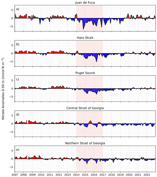
Nitrate anomalies were mostly consistent across all depth layers (0–50, 50–150 and >150 m; Figs. 6–7, S3–S4). Positive nitrate anomalies were observed in all regions from 2007 until approximately mid-2013 with the exception of a slight decrease in nitrate during the winter/early spring of the 2010 El Niño in JdF, Haro Strait, and Puget Sound (Fig. 6). The strongest negative nitrate anomalies occurred in the JdF region during the NEP-MHW years (Figs. 6–7). In comparison, the Central SoG had the weakest negative nitrate anomalies during the NEP-MHW years wherein nitrate was periodically replenished into the surface waters (Figs. 6d, 7d). Periodic increases in nitrate were also observed at depth in the Central SoG in 2017. Following the NEP-MHW years of 2014–2017, two distinct patterns were observed: nitrate anomalies returned to predominantly positive values in early 2020 in the JdF, Haro Strait, and PS regions; in contrast, nitrate anomalies in the Central and Northern SoG remained predominantly negative until end of 2022. Surface nitrate anomalies were significantly correlated with the NPGO in the Central SoG (r=0.49, p<0.001), but not the SOI (r=0.11, p=0.12; Table 1), whereas surface nitrate anomalies in the JdF region were correlated with the SOI (r=0.34, p<0.001), but not the NPGO (r=0.09, p=0.21).

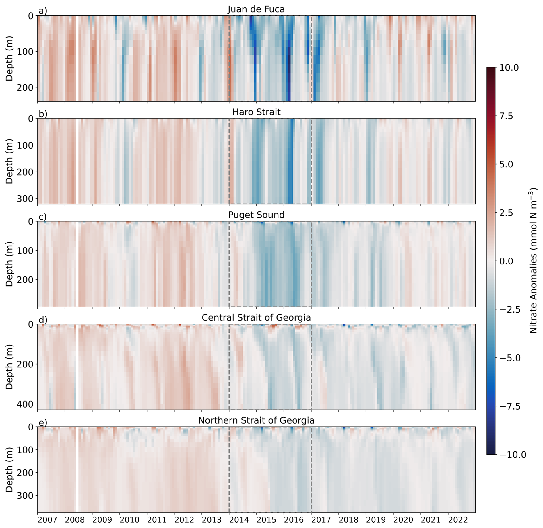
Figure 6 Model-based nitrate anomalies versus depth in the different sub-regions of the Salish Sea from 2007 to 2022. Red indicates positive nitrate anomalies and blue represents negative nitrate anomalies. The NEP-MHW of 2014–2017 is outlined with dashed grey lines. Note that the vertical (depth) scales vary, reflecting the maximum depth of each region. White line is missing data from June 2008.

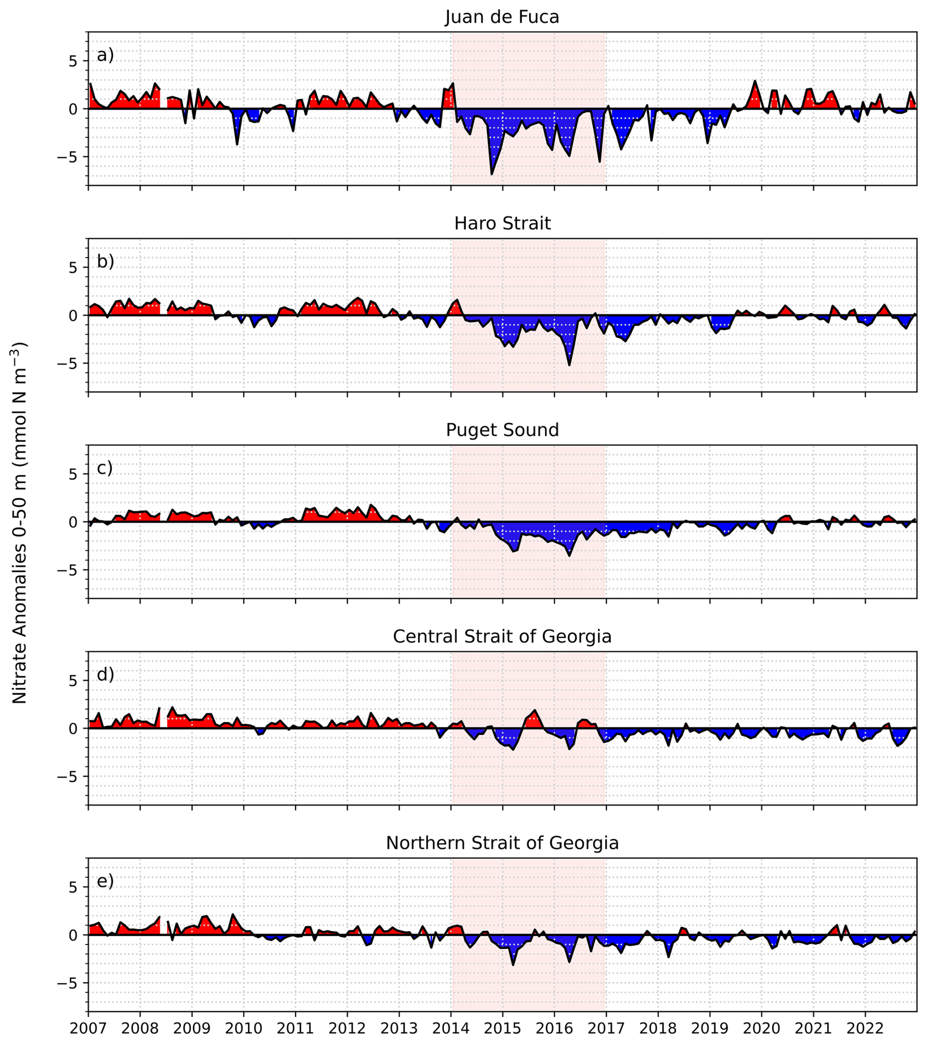
Figure 7 Mean model-based 0–50 m nitrate anomalies in the different sub-regions of the Salish Sea from 2007 to 2022. Nitrate anomalies for the 50–150 and 150 m to bottom depth ranges are provided in the Supplement (Figs. S3–S4).

3.1.4 Phytoplankton

During the NEP-MHW, prolonged positive anomalies in diatom concentration were seen at the beginning of 2015 in the JdF region; however stronger positive anomalies in diatoms persisted from 2018 to 2020 (Figs. 8a, S5a). In addition, a strong positive anomaly (50 % increase compared to the mean) in nanoflagellates, the concentration of which is typically relatively low in JdF, was observed in 2015 (Figs. 8b, S5b). Diatom growth in the JdF region was less limited by temperature during the 2010 El Niño event and the NEP-MHW years of 2014–2017 (positive values for the purple lines; Fig. 9a). In addition, while the JdF region is generally nutrient replete year round, the decrease in nitrate associated with the NEP-MHW years resulted in a slight increase in nitrate limitation on diatom growth compared to the climatology (negative values for blue and green lines; Fig. 9b), but this limitation was not strong enough to inhibit photosynthetic growth of diatoms at any point during the study period in the JdF region.

In contrast, diatom concentrations decreased while nanoflagellates increased in the Central SoG during the NEP-MHW years with negative diatom anomalies continuing to persist for longer durations each year until the end of 2022 (Figs. 8b, d; S6a, b). Also evident was that diatoms during warm-phase NPGO years peaked earlier in the season, and for shorter durations, relative to the pre-MHW period (Figs. 8b, S6a). Our limitation plots indicated that diatom growth in this region was occasionally limited by temperature (Fig. 9a); however, the Central SoG periodically experienced negative temperature anomalies in the 0–50 m depth layer during the NEP-MHW of 2014–2017 (Fig. 4d), thus temporarily alleviating any temperature limitation during the main NEP-MHW years. Overall, nitrate was the most limiting to diatom growth during the summer months in the Central SoG (Fig. 9b).

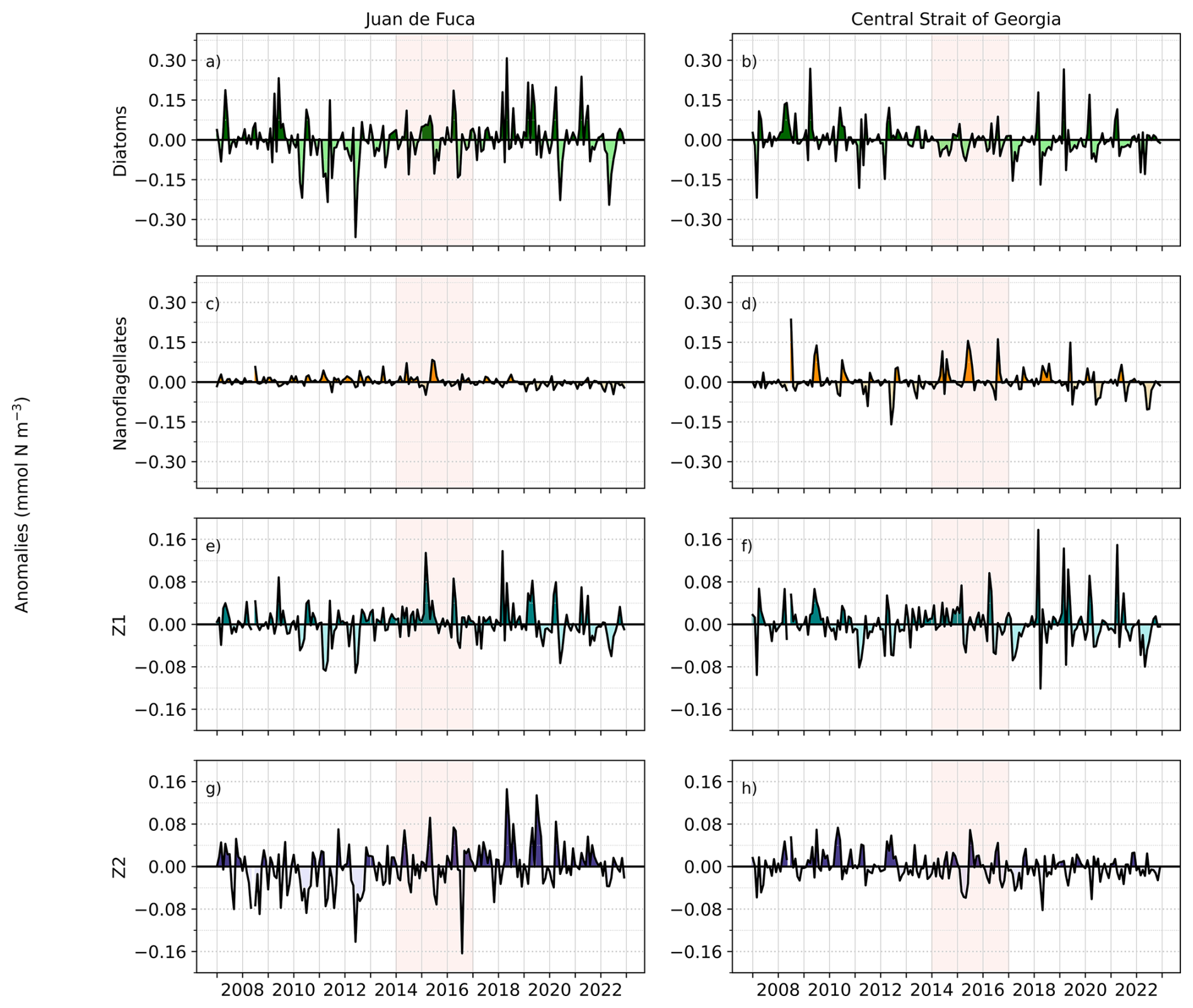
Figure 8 Anomalies in mean model-based 0–50 m biological parameters (diatoms, nanoflagellates, Z1, and Z2 zooplankton in the Juan de Fuca and Central Strait of Georgia regions from 2007 to 2022. For anomalies including the seasonal cycle see Figs. S5–S6.

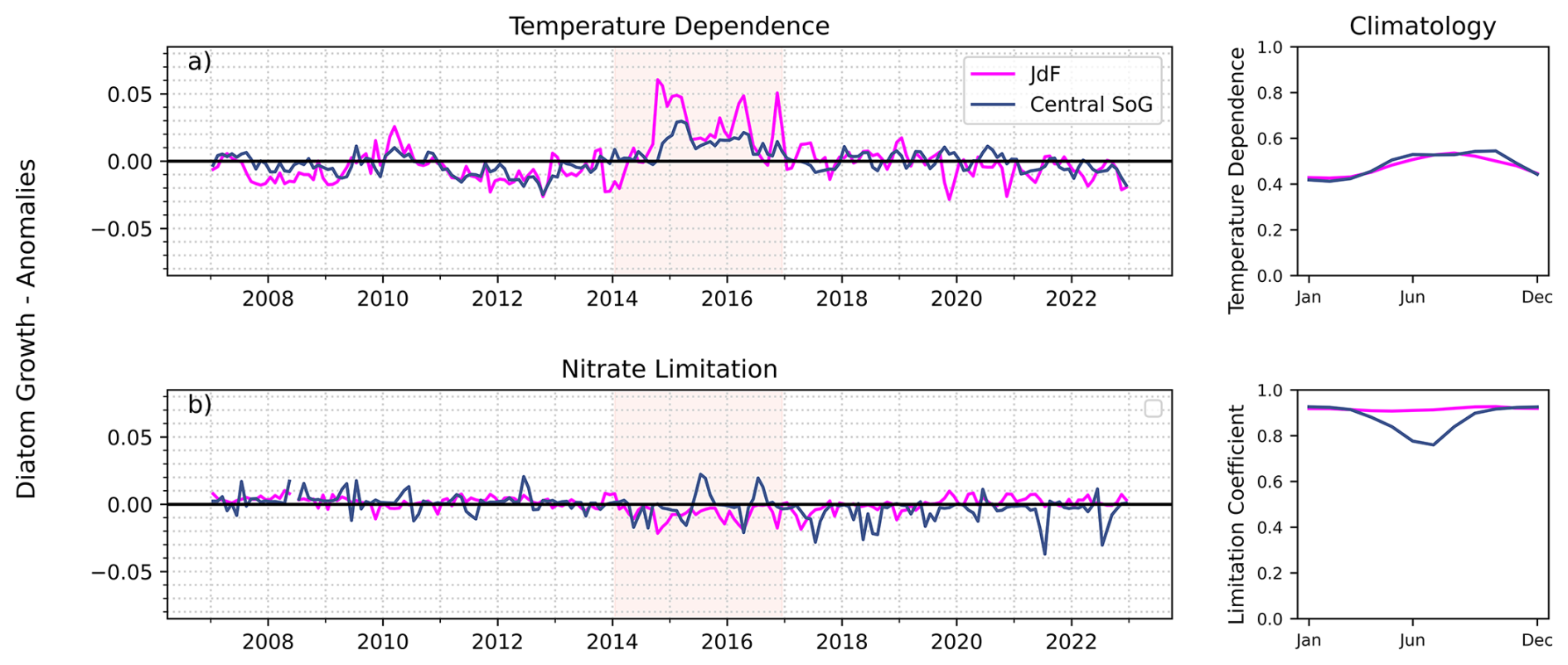
Figure 9 Left panels: anomalies in (a) temperature dependence, and (b) nitrate limitation on diatom growth in the 0–50 m depth layer compared to the 16 year climatology (2007–2022; right panels) in the Juan de Fuca and Central Strait of Georgia regions. Positive anomalies mean less limitation or temperature dependence compared to climatology; negative anomalies reflect more limitation or temperature dependence.

3.1.5 Zooplankton

Anomalies in Z1 and Z2 zooplankton concentrations followed patterns like those observed for diatom anomalies in the JdF region (Figs. 8, S5). No clear variations in either of the zooplankton classes were observed in relation to the NEP-MHW years; however, stronger positive anomalies of Z1 zooplankton occurred from about 2014 to 2020. This pattern was also evident for Z2 zooplankton in the JdF where mostly negative anomalies persisted from 2007 to 2014 and then switched to mostly positive anomalies for the remainder of the study period (Fig. 8g). Z1 anomalies closely followed the diatom pattern in the Central SoG, but negative anomalies in Z2 concentration predominated from 2014 to 2022 (Figs. 8f, h; S6), coinciding with warm-phase NPGO years. Given that spatial variability in Z2 biomass in the model reflects differences in the spatial distribution of their prey, our results suggest that zooplankton experienced better feeding conditions in the JdF region compared to the Central SoG during the latter half of our study period.

3.2 Model and Observation Comparisons

In JdF, our results showed that the model did not capture the range of observed 0–10 m nitrate concentrations; however, the seasonal cycles of model versus observations were comparable (Fig. 10a). The range of nitrate concentrations in the model was 12–26 µM whereas observation values ranged from 5–30 muM, including very low observation values during the NEP-MHW years. Seasonal peaks in Chl a in the observations were generally captured by the model (Fig. 10b). Observed Chl a ranged between 0.2 and 12 mg m⁻³ but model Chl a had a smaller range of 0.6 to 3 mg m⁻³. Unfortunately, few zooplankton observation samples were available in the JdF region prior to 2014, which limited our comparison (Fig. 10c). That said, model zooplankton (Z1 and Z2 combined) values were always within the range of observed values although the model failed to capture some of the extreme values that can be expected in observation data due to the patchiness of zooplankton sampling.

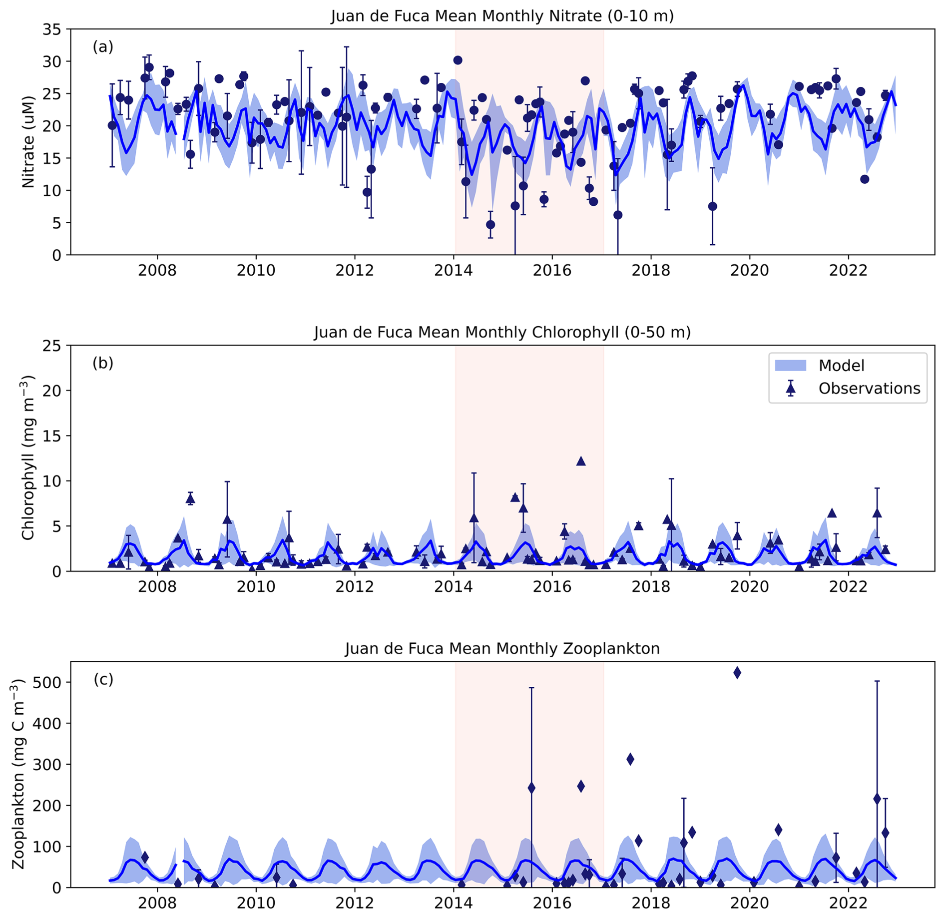
Figure 10 SalishSeaCast Model comparison with observation data for the Juan de Fuca region for (a) 0–10 m nitrate, (b) 0–50 m chlorophyll a and (c) full water column zooplankton. Chlorophyll a observation data were compared to the sum of model diatoms and nanoflagellates multiplied by a Chl : N of 2. Zooplankton observation data were compared to the sum of model Z1 and Z2 zooplankton biomass. Dark blue lines indicate mean model values with combined spatial (grid point) and temporal (daily) standard deviations in light blue shading. Symbols for observation data are the mean monthly value with whiskers showing standard deviations.

In the Central SoG, model nitrate showed better agreement with observed values; however, the model failed to capture the high Chl a peaks that occurred throughout the observation time series (Fig. 11a, b). Observation zooplankton data were more comprehensive in this region, thus allowing for more accurate ground truthing. Our results showed that model zooplankton biomass was higher than observations over the course of our study period (Fig. 11c). Better agreement between model and observations was evident after 2015 corresponding to increased temporal resolution of observation sampling (Fig. 11c).

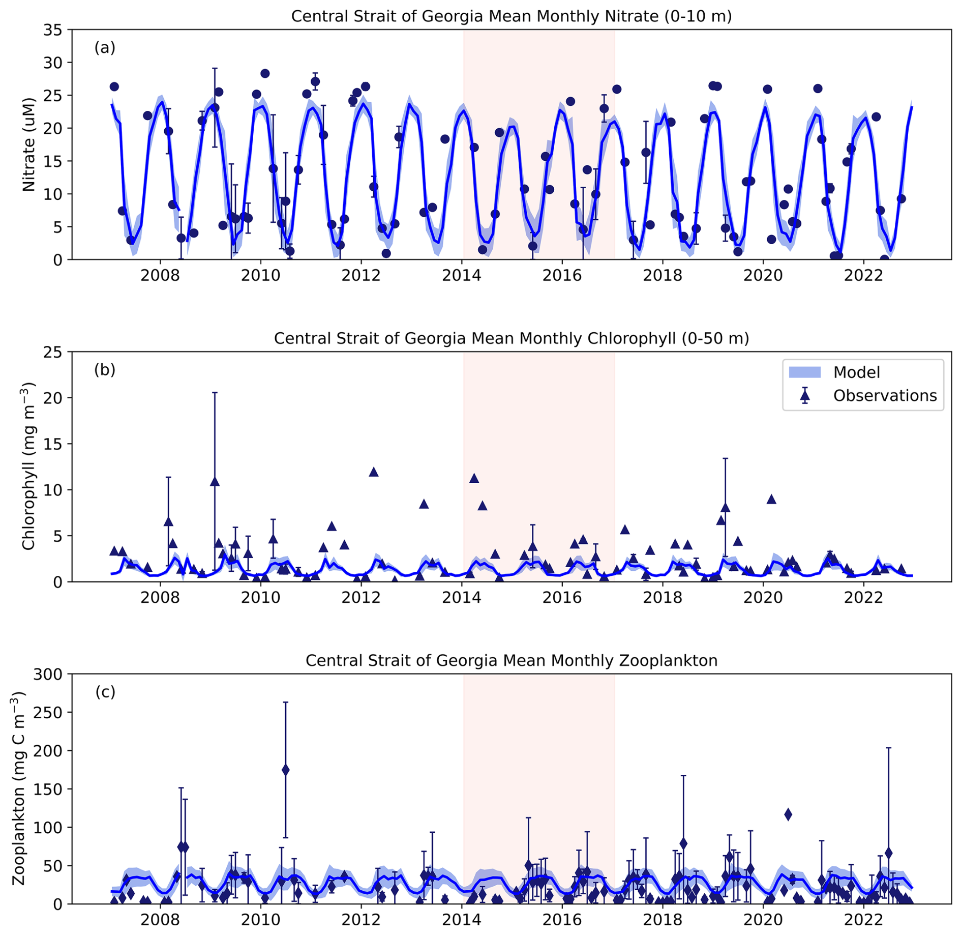
Figure 11 SalishSeaCast Model comparison with observation data for the Central SoG region for (a) 0–10 m nitrate, (b) 0–50 m chlorophyll a and (c) full water column zooplankton. Note that the y-axis range for zooplankton differs from the zooplankton range presented in Fig. 10c for JdF. Chlorophyll a observation data were compared to the sum of model diatoms and nanoflagellates multiplied by a Chl : N of 2. Zooplankton observation data were compared to the sum of model Z1 and Z2 zooplankton biomass. Dark blue lines indicate mean model values with combined spatial (grid point) and temporal (daily) standard deviations in light blue shading. Symbols for observation data are the mean monthly value with whiskers showing standard deviations.

Significant differences in the JdF region were found between pre-MHW, MHW, and post-MHW years for model nitrate (F(2, 13)=4.59, p<0.05; Fig. 12a). Tukey's HSD indicated significant differences between pre-MHW and MHW (p<0.05) with higher model nitrate during the pre-MHW period. No significant differences were found for observation nitrate (F(2, 13)=3.36, p<0.07; Fig. 12b); however, model and observation data showed similar patterns with a decrease in nitrate occurring during MHW years. In comparison, significant differences were found for observation Chl a (F(2, 13)=5.18, p<0.05) with Tukey's HSD showing significant differences between pre-MHW and MHW (p<0.05) and between pre-MHW and post-MHW (p<0.05) with pre-MHW Chl a being lower (Fig. 12c). No significant differences were found for model Chl a (F(2, 13)=2.18, p=0.16) and model and observation results showed slightly different patterns in response during MHW and post-MHW years (Fig. 12c, d). Specifically, both datasets showed an increase in Chl a from pre-MHW to MHW years; however, Chl a biomass remained high in observations whereas model Chl a decreased post-MHW. Although model zooplankton showed a significant difference in JdF region between pre-MHW, MHW, and post-MHW years (F(2, 13)=4.23, p<0.05), no significant differences were found for observed zooplankton (F(2, 10)=1.53, p=0.26; Fig. 12e, f). Tukey's HSD indicated a significant increase in model zooplankton from pre-MHW to MHW years (p<0.05). We note that the limited availability of zooplankton observations prior to 2015 hindered our ability to adequately assess the effects of the NEP-MHW on in situ zooplankton in this region.

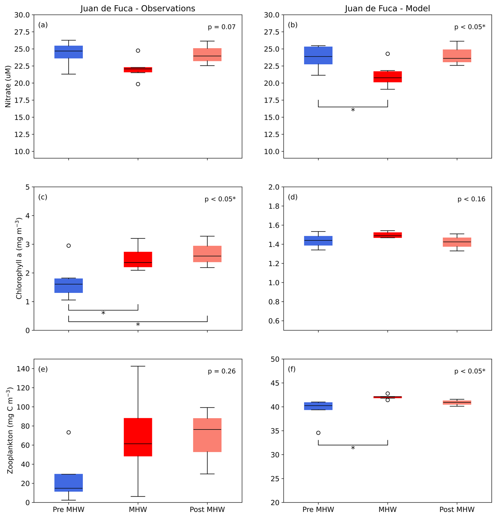
Figure 12 Mean 0–10 m nitrate concentration, 0–50 m chlorophyll a biomass, and full water column zooplankton biomass pre-marine heatwave years (Pre MHW; 2007–2013), marine heatwave years (MHW; 2014–2019), and post-marine heatwave years (Post MHW; 2020–2022) for observation and data in the Juan de Fuca Strait region. Vertical scales differ between observed and modelled chlorophyll a and zooplankton to account for the higher and more variable observations, as shown in previous model evaluations (Olson et al., 2020; Suchy et al., 2023). ^*significant at p<0.05; ${}^{**}$ significant at p<0.01; ${}^{***}$ significant at p<0.001.

In the Central SoG, model nitrate was significantly different between pre-MHW, MHW, and post-MHW years (F(2, 13)=18.57, p<0.001; Fig. 13a, b). Tukey's HSD showed lower nitrate values were observed in pre-MHW years compared to both the MHW (p<0.001) and post-MHW (p<0.01) periods. No other significant effects of the marine heatwave were seen in either model or observation data. We suspect that these results are mainly due to the timescales over which our comparisons were made. For example, while the monthly model results showed a notable decrease in diatom biomass during the NEP-MHW years and earlier peaks in diatom biomass post-MHW (Figs. 8, S6), this variability tended to occur within seasonal timescales.

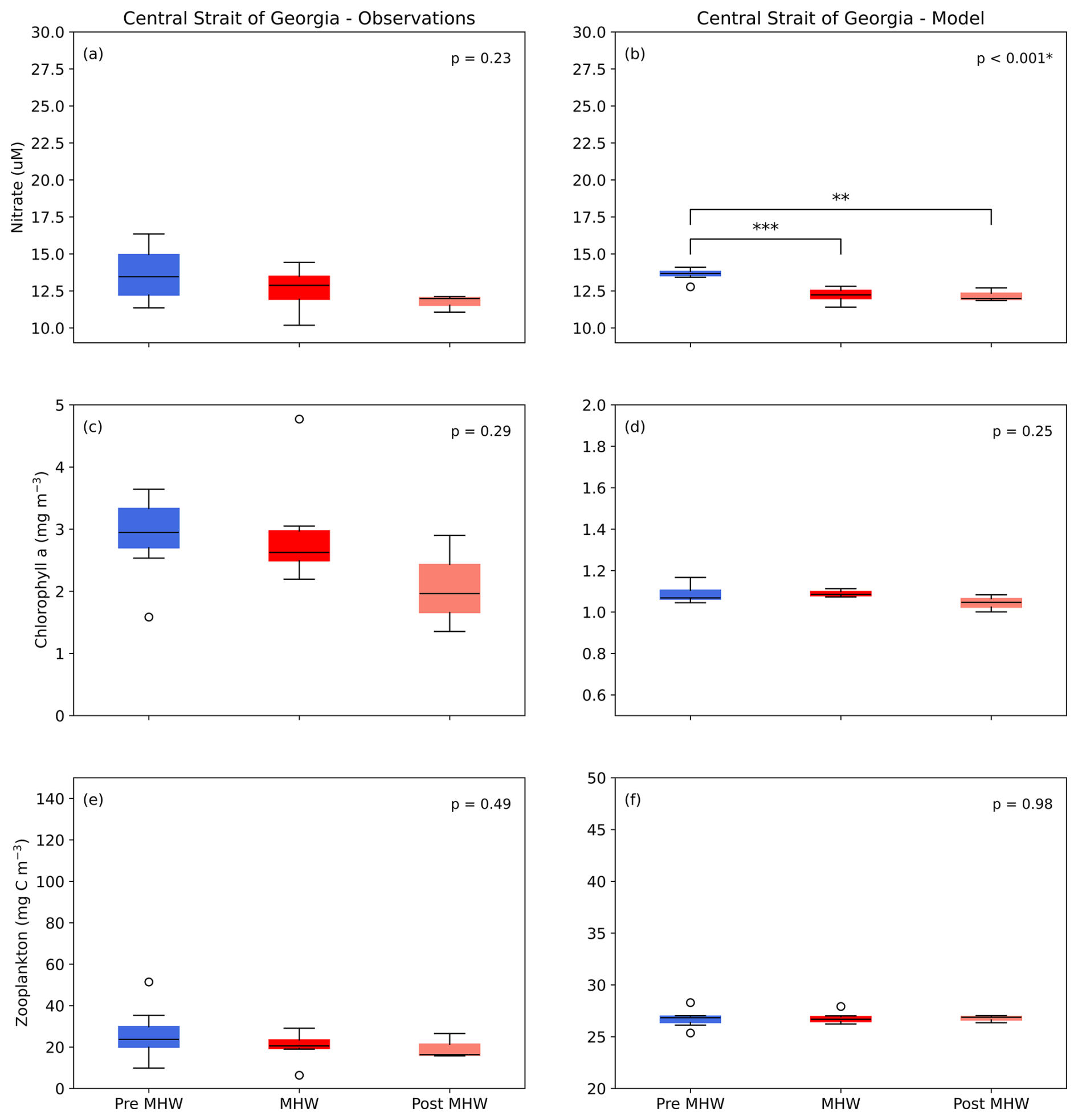
Figure 13 Mean 0–10 m nitrate concentration, 0–50 m chlorophyll a biomass, and full water column zooplankton biomass pre-marine heatwave years (Pre MHW; 2007–2013), marine heatwave years (MHW; 2014–2019), and post-marine heatwave years (Post MHW; 2020–2022) for observation and data in Central SoG region. Vertical scales differ between observed and modelled chlorophyll a and zooplankton to account for the higher and more variable observations, as shown in previous model evaluations (Olson et al., 2020; Suchy et al., 2023). ^* significant at p<0.05; ${}^{**}$ significant at p<0.01; ${}^{***}$ significant at p<0.001.

4 Discussion

4.1 Physical and chemical responses to the NEP-MHW

4.1.1 Temperature

Modelled results from this study suggest that different types of warming events existed simultaneously within the Salish Sea during the NEP-MHW years and beyond. The strongest temperature signals of the NEP-MHW were found in the surface (0–50 m) layer of the JdF, Haro Strait, and PS regions (maximum anomalies of 2.0 °C for JdF and 1.5 °C for both Haro Strait and PS; Fig. 4. Temperature anomalies in the surface layer of these regions remained predominately positive into 2019 when a second MHW occurred in the Northeast Pacific (Amaya et al., 2020; Chen et al., 2021). Warming in the intermediate (50–150 m) and deep (150 m to bottom) layers in the JdF region exhibited patterns similar to those in the upper water column; however, warm anomalies in these deeper layers arrived in pulses during the winter months from 2014–2017 and again in winter 2019 (Figs. S1a, S2a). This inflow of warmer water into the Salish Sea during the NEP-MHW years was primarily driven by shallow source waters entering the JdF (Beutel et al., 2025). Cooler waters (negative temperature anomalies) were introduced into the JdF region in the intermediate and deep layers during spring and summer throughout the NEP-MHW period, likely partially driven by seasonally stronger estuarine circulation.

In contrast, the warming response in the SoG during the NEP-MHW years was muted, with maximum anomalies of only 1.1 °C in both the Central and Northern SoG (Fig. 4d, e). Positive temperature anomalies appeared at the end of 2013 in the surface layer of the SoG, which was earlier than the NEP-MHW reported for coastal regions but consistent with the initiation of the NEP-MHW in the Gulf of Alaska (Bond et al., 2015). Most notably, warming persisted in the surface waters of the Central SoG until the end of our study period in 2022, suggesting that warming in the SoG likely originated from sources other than the NEP-MHW (e.g., atmospheric heating). Prolonged warming was also observed in the deeper waters of the SoG beyond the NEP-MHW years with no evidence of cooler water intrusions as was seen in the JdF region (Figs. S1d, S2d). The prolonged deep water warming was previously shown in a modelling study of the Salish Sea (Khangaonkar et al., 2021) as well an observation study from Rivers Inlet, BC (Jackson et al., 2018). Jackson et al. (2018) suggested that warm water anomalies may be removed from deep fjords either through mixing with overlying colder waters or via renewal events when colder water enters over the sill. In the present study, our model results indicated that warm water persisted in the 0–50 m layer following the NEP-MHW in the Central SoG with cooling of the deep basin waters occurring only after negative temperature anomalies appeared in the intermediate layer of the JdF (Fig. S1), which subsequently flow into the SoG (Pawlowicz et al., 2007; Allen et al., 2025).

4.1.2 Nitrate

Similar to the temperature signal, the strongest negative nitrate anomalies during the NEP-MHW years occurred in the JdF region followed by Haro Strait and PS (Figs. 6, 7). While positive nitrate anomalies returned to the JdF, Haro Strait, and PS regions after 2019, the SoG exhibited lower nitrate concentrations until the end of our study period in 2022, especially in the intermediate and deep layers. Furthermore, weaker nitrate anomalies were seen in the surface layer (0–50 m) of the Central SoG wherein nitrate was periodically replenished (Fig. 7d), likely due to wind-induced upwelling events (Moore-Maley and Allen, 2022). An increase in nitrate was also observed at depth in the Central SoG in 2017 (Figs. 6, S4). This contrasting pattern in the nitrate signal can be partly explained by the unique ways in which nitrate is entrained back into and/or recycled in the deep basin of the strait. Specifically, due to the intense mixing in the Haro Strait region, a large portion of the water leaving the SoG eventually gets mixed back into the region (Pawlowicz et al., 2007; Ianson et al., 2016; Allen et al., 2025). In addition, nitrate is constantly being regenerated within the SoG due to high biological productivity (Ianson et al., 2016; Sutton et al., 2013).

Overall, the largest source of nutrients into the Salish Sea is from the Pacific via estuarine inflow into the Juan de Fuca Strait with direct inputs via rivers and streams contributing a relatively small amount of dissolved nutrients into the system (Mackas and Harrison, 1997; Sutton et al., 2013). The aforementioned modelling study of the Salish Sea by Khangaonkar et al. (2021) found that increased freshwater flow during the NEP-MHW years resulted in higher nutrient concentrations due to increased exchange flows relative to their pre-MHW reference year (2013). Here, an increase in Fraser River discharge was not seen during the NEP-MHW years relative to our climatology (Fig. 2). In fact, the highest Fraser River discharge occurred in 2011, 2012, and 2020, years wherein there were no substantial increases in nitrate. This discrepancy between modelling studies of the same region can be explained by the different reference periods, i.e., a single year in Khangaonkar et al. (2021) versus the climatology of 2007–2022 used in this study. We note that in the SoG estuarine flow is a function of river flow (primarily the Fraser River), offshore upwelling, and the characteristics of the water currently sitting in the surface and intermediate layers within the SoG (Allen et al., 2025). Instead, our results suggest that the nitrate anomalies throughout the water column are linked to larger-scale, basin-wide processes with periodic influences of other local methods of nutrient delivery.

4.2 Regional connections to large-scale climate indices

Results from this study revealed that warming in the Salish Sea may be driven by atmospheric changes and large-scale climate patterns acting either simultaneously (e.g., El Niño events corresponding with the NEP-MHW years in the JdF region) or operating somewhat independently of the NEP-MHW (e.g., the NPGO exerting the strongest influence on local conditions in the Central SoG). Temperature anomalies for all depth layers in the JdF region were significantly and negatively correlated to the SOI but not to the NPGO (Table 1). In the Central SoG, temperature anomalies throughout the water column were also correlated with the SOI, but the surface and intermediate waters showed stronger negative correlations to the NPGO. We hypothesize that the JdF region, with its direct connection to the open ocean and high mixing is more strongly influenced by the shorter term variability of the SOI. In contrast, the deep basin of the Central SoG is semi-enclosed and is more likely to retain physical and chemical signals longer than areas with stronger mixing and is affected by regional scale forcing from multiple sources (atmospheric, open ocean, and rivers). Previous work in the Central SoG and, in particular, the surface waters, have shown that this region may be affected by both direct effects of large-scale climate indices as well as by indirect effects through variability in local conditions, e.g., river discharge (Suchy et al., 2019), winds (Suchy et al., 2025a), SST and winds (Perry and Masson, 2013), river discharge and winds (St. John et al., 1993).

El Niño events off of the west coast of Vancouver Island have been associated with a reduction in north-westerly winds and thus in upwelling strength (Harris et al., 2009). Upwelling-favourable winds (equatorward) are typically present along the west coast of Vancouver Island from late March to September bringing cold, nutrient-rich water to the surface (Thomson, 1981). During winter (October through early March) an abrupt reversal of the prevailing winds produces downwelling-favourable conditions. While winds directly relevant to upwelling on the west coast of Vancouver Island are outside of our SalishSeaCast model domain, the effects of downwelling-induced mixing were noted by Khangaonkar et al., (2021) for the continental shelf from 2014 to 2016, wherein temperature anomalies were seen throughout the water column.

Nitrate concentrations in the JdF, Haro Strait, and PS regions were typically lower during El Niño years. Globally, marine heatwaves (in the form of El Niño events) have been shown to suppress nutrients in some regions by weakening the upwelling of nutrient-rich waters (Hayashida et al., 2020). The association of El Niño events with anomalously weak upwelling and a subsequent reduction in nutrients has been observed in both the California Current System (Jacox et al., 2015) and off the west coast of Vancouver Island (Harris et al., 2009). Since upwelling fluxes are the largest offshore source of nutrients near the mouth of Juan de Fuca Strait (Peña et al., 2019), we expect the effects of variability in upwelling to propagate into the Salish Sea via the source of water entering through the intermediate depth layer (Beutel and Allen, 2024). The Northeast Pacific was found to be warmer and less nutrient-rich during El Niño events (Whitney et al., 1998), which supports our findings of winter intrusions of warm, lower-nitrate waters in the JdF, Haro Strait, and PS regions during the stronger El Niño events (negative SOI) of 2009–2010 and 2015–2016 (Fig. 2). Indeed, the lower nitrate concentrations observed during NEP-MHW years have been attributed to the increased inflow of shallow, nutrient-poor source waters into the region, the volume of which is directly impacted by the seasonal wind forcing resulting in upwelling/downwelling events (Beutel et al., 2025).

While we suspect that temperature and nitrate patterns propagating into the JdF, Haro Strait, and PS regions resulted from the combined effects El Niño and the NEP-MHW, given their proximity to the open ocean boundary and sensitivity to changes in source waters, nitrate concentrations at all depth layers in the Central SoG were tightly coupled with the NPGO (Table 1). The NPGO is associated with basin-wide fluctuations in salinity, nutrients, and chlorophyll a concentrations in the Northeast Pacific (Di Lorenzo et al., 2008). Previously, negative nitrate anomalies in the Central SoG were linked to weaker winds during warm-phase NPGO years which prevented nutrients from being mixed into the surface waters during warm-phase years (Suchy et al., 2025a). In the present study, the shift to negative nitrate anomalies in the SoG (Figs. 6–7) was associated with a shift in the NPGO index to its negative (warm) phase in October 2013 (Fig. 2a) and with weaker winds (Fig. 2b).

4.3 Cascading food web processes in response to the NEP-MHW

We discuss the cascading processes by which variability in temperature and nitrate propagated through the food web by focussing on the two main regions representing the different types of heatwaves observed: (i) the JdF region, which was strongly influenced by the co-occurrence of the 2014–2017 NEP-MHW and El Niño-related warming events, and (ii) the Central SoG wherein temperature anomalies were weaker and nitrate was strongly coupled to the NPGO, thus masking the effects of the 2014–2017 NEP-MHW.

4.3.1 Juan de Fuca

Anomalies of phytoplankton can be positive or negative in response to marine heatwaves depending on which resource (e.g., light, nutrients) is the most strongly limiting (Hayashida et al., 2020). In general, the JdF region is cooler relative to the rest of the Salish Sea (Thomson, 1981) and diatoms tend to dominate the phytoplankton community year-round (Nemcek et al., 2023). The climatological mean water temperature in the 0–50 m layer of the JdF region in this study was 7.1 °C and the maximum water column temperature was 12.3 °C. Since the optimal temperatures for diatoms and nanoflagellates are set in the model at 12 and 18 °C, respectively, the warming of up to 2.0 °C during the NEP-MHW in this region was favourable for the growth of both phytoplankton groups (Fig. 8). Indeed, we observed a larger effect on the temperature dependence of diatom and nanoflagellate growth (positive anomalies; Figs. 9a, S7) during the NEP-MHW compared to nitrate limitation (negative anomalies, Fig. 9b). Although phytoplankton biomass was slightly elevated during NEP-MHW years, even higher diatom biomass occurred during the second MHW in 2018 and 2019 (Fig. 8).

It is important to note that the negative nitrate anomalies in the JdF region during the NEP-MHW were not associated with increased stratification as this region is almost constantly mixed relative to the SoG (Fig. 5a; Thomson, 1981). Furthermore, the decrease in nitrate during NEP-MHW years was not a result of increased phytoplankton consumption due to higher primary productivity. The maximum primary productivity anomaly in the model during the NEP-MHW years in the 0–50 m layer in the JdF region was in May and was 0.03 mmol N m⁻³ d⁻¹; the nitrate anomaly over the same depth and time period was −2.1 mmol N m⁻³. Assuming a transit time of approximately 2.3 d in this region (Thomson et al., 2007), maximum excess nitrate drawdown in the NEP-MHW years from primary productivity was <5 % of the observed nitrate anomaly and thus insufficient to explain the nitrate decrease. Despite the lower than average nitrate concentrations seen during the NEP-MHW, nitrate concentrations for both the model and observation data were always >5 µM (Fig. 10a), thus indicating that nitrate was always replete in the JdF region.

During the NEP-MHW years and thereafter, variability in temperature and nitrate affected modelled zooplankton primarily through changes in Z1 and Z2 prey (Fig. 8). For example, Z1 biomass followed closely the diatom and nanoflagellate patterns, as expected given that this zooplankton class represents smaller zooplankton taxa with high grazing rates (e.g., nauplii, small copepods). Z1 increased during the NEP-MHW years and again during the second MHW due to its feeding preference for both nanoflagellates and diatoms, which both responded favourably to the surface warming. In comparison, Z2 is more constrained by model settings as it represents the model closure term, which is more nuanced than in other biogeochemical models in the region (see Suchy et al., 2023). Specifically, at any given time, the Z2 concentration is distributed throughout the model domain in proportion to its prey; however, the temporal variability of Z2 is also constrained by a prescribed seasonal cycle. Therefore, in contrast to Z1, Z2 dynamics are not driven solely by local conditions. Nevertheless, the highest Z2 biomass was seen immediately following the NEP-MHW, in response to the increased availability of both diatoms and Z1 which are the preferred prey of this class representing larger-bodied taxa with longer life cycles (e.g., overwinter copepods, euphausiids).

4.3.2 Central Strait of Georgia

The Central SoG is one of the warmest regions of the Salish Sea with mean and maximum climatological temperatures in the 0–50 m layer of 9.9 and 19.5 °C, respectively, in this study. The largest decrease in diatom biomass occurred during the NEP-MHW, corresponding to an increase in nanoflagellates (Fig. 8). The Central SoG region typically exhibits a strong spring bloom of diatoms, followed by a shift to a mixed flagellate community when nitrate becomes limiting in the summer (Nemcek et al., 2023). Our modelled results showed weak diatom blooms and a predominance of nanoflagellates earlier in the year during the NEP-MHW. Although nitrate limitation anomalies on diatom growth were similar between the Central SoG and the JdF regions during the NEP-MHW years, the impact is different due to the base nitrate limitation shown in the climatology (Fig. 9b). As the Central SoG is generally nitrate limited in summer, a negative anomaly has a direct impact on growth. However, in the JdF region, nitrate is not limiting and a negative anomaly has no direct impact on diatom growth. Unlike the well-mixed JdF region, negative nitrate anomalies persisted in the Central SoG during the NEP-MHW years coinciding with higher stratification (Fig. 5d) and sustained weak winds (Fig. 2b), which likely prevented nutrient-replenishment into the surface waters (Moore-Maley and Allen, 2022; Suchy et al., 2025a).

Both warming and low nitrate persisted in the 0–50 m layer in the Central SoG from the late 2013 until the end of our study period (2022) correlating with warm-phase NPGO years. In addition, nitrate was consistently limiting to diatom growth in the upper 50 m from ∼ 2017 to 2022 (blue line negative values; Fig. 9b), which resulted in changes in the seasonal succession of phytoplankton in the model. Specifically, diatoms peaked earlier and for shorter durations after 2017. Earlier bloom timing in the Central SoG (Suchy et al., 2022) and a shift to smaller phytoplankton in the California Current System (Barth et al., 2020; Fischer et al. 2020), have previously been linked to warm-phase NPGO years.

The timing of the spring diatom bloom, in turn, has significant effects on zooplankton biomass in the region (Perry et al., 2021; Suchy et al., 2022). The biomass of the zooplankton community in the Central SoG is typically dominated (>75 %) by medium and large copepods (e.g., Metridia and Calanus spp., Neocalanus plumchrus), euphausiids (Euphausia pacifica), and amphipods (e.g., Themisto pacifica; Perry et al., 2021), which are mainly represented by our Z2 model class. Our results showed lower Z2 biomass after the NEP-MHW (Fig. 8h) and higher biomass of the Z1 model class (Fig. 8f), which represents smaller-sized zooplankton taxa. Comparable results have also been shown in recent observation studies wherein lower crustacean zooplankton biomass was associated with warm years with early chlorophyll a blooms (Suchy et al., 2022). Similarly, Perry et al. (2021) reported low zooplankton biomass in 2014 in the Central SoG but not for the other NEP-MHW years. The contrasting results we observed in the modelled zooplankton response between the Central SoG and the JdF regions suggest that post-NEP-MHW conditions were more favourable for Z2 in the JdF region, where nitrate-replete waters supported diatom growth. In the Central SoG, persistently low nitrate favoured the nanoflagellate-Z1 pathway instead. Together, these differences highlight the need for comprehensive, long-term regional analyses of lower trophic level dynamics throughout the Salish Sea.

4.4 Model-observation comparisons

Our attempts to determine if the marine heatwave-related patterns found for the model were also evident in the observation data were met with some challenges. For example, to compare with observation data we needed to compromise on both spatial and temporal scales due to differences in sampling resolution. Spatially, we expanded the extent of the JdF and Central SoG observations beyond the initial model boxes provided in Fig. 1 to ensure an adequate number of observations were available for comparison with model results (Fig. S8). Temporally, since observation data were not consistently available at the monthly spatial resolution used for model output, particularly in the JdF region, we used annual mean values for comparisons between the observation and model datasets prior to grouping into pre-MHW, MHW, and post-MHW years, which smoothed out the important finer-scale seasonal or monthly patterns shown in the modelled plankton results discussed above.

Nevertheless, significant differences were seen in modelled nitrate concentrations between pre-MHW, MHW, and post-MHW years in the JdF region with the lowest nitrate concentrations occurring during the MHW years (Fig. 12b). Observation data showed a similar pattern but the results were not significantly different (Fig. 12a). The model failed to capture the low observation nitrate values during the NEP-MHW years (Fig. 10), likely due to spatial differences in our comparisons. For example, observation sampling locations during the NEP-MHW years were mainly limited to the deepest part of the JdF region, whereas the model values were averaged over the entire JdF box (Fig. 1). In comparison, although the seasonal cycle of model and observation nitrate showed better agreement in the Central SoG (Fig. 11), significant differences in nitrate concentrations between pre-MHW, MHW, and post-MHW years were seen only in the model results (Fig. 13b).

Comparisons of modelled and observed chlorophyll a and zooplankton between pre-MHW, MHW, and post-MHW years were more variable. Lower biomass of both groups was observed pre-MHW, but not post-MHW (Fig. 12c, e). Phytoplankton biomass is notoriously patchy, which is not reflected in the model (see Olson et al., 2020). As a result, sampling location and timing may skew observation results considerably compared to modelled results based on hourly outputs. Although modelled zooplankton biomass in the JdF region was significantly higher during the MHW compared to the pre-MHW period (Fig. 12e, f), the lack of zooplankton observations prior to 2015 severely affected our ability to interpret the in situ response of the NEP-MHW in the JdF. In comparison, more observation data were available in the Central SoG (Fig. 11) where no significant differences in chlorophyll a or zooplankton were detected between pre-MHW, MHW, and post-MHW years in either the model or the observations (Fig. 13). These results support our hypothesis that the NEP-MHW was not the main warming signal causing cascading food web changes in the Central SoG.

5 Conclusions

Our model results showed that the strongest physical signatures of the NEP-MHW were evident in the JdF region, followed by Haro Strait and Puget Sound. The positive temperature anomalies and negative nitrate anomalies characteristic of the NEP-MHW years were also present in these regions during the El Niño of 2009–2010. Given that the waters in the JdF region are nutrient replete and, on average, cooler compared to other regions, the increased temperatures associated with the NEP-MHW favoured phytoplankton growth and a resulted in a subsequent increase in zooplankton biomass. In contrast, nitrate had little to no effect on the phytoplankton growth as nitrate was never limiting in this region. The JdF region experienced intrusions of cooler water at depths >50 m both during and after the NEP-MWH. In contrast, warming associated with the NEP-MHW had less of an impact on plankton in the Central SoG. Although positive temperature anomalies were prevalent during the NEP-MHW years in this region, they were weaker compared to other regions and remained anomalous in the surface until the end of our study period. Colder water only entered the deep layers of the SoG after consistent negative temperature anomalies were observed in the intermediate waters of the JdF region. In contrast to the JdF region, both temperature and nitrate were strongly linked to the NPGO index in the Central SoG. A decrease in diatom concentration was observed during warm-phase NPGO years, including the NEP-MHW years, likely due to the nitrate limitation associated with weaker wind-driven resupply of nutrients to the surface waters. Future studies using model sensitivity analyses to tease apart the effects of MHWs on biogeochemical responses relative to natural variability are warranted but were beyond the scope of this study. Comparison of model and observation data highlighted a common challenge faced by researchers attempting to use a combined model-observation approach: mismatches in spatial and temporal scales led to limitation in our analyses. Nevertheless, the findings presented here also highlight the need for comprehensive in situ sampling programs as model tuning improves with increased observation data availability. The regional analysis presented in this study revealed that multiple types of marine heatwaves can impact different sub-regions within the same coastal water body and, as a result, have unique repercussions throughout the food web.