Are ghost forest trees a substantial source of methane from reservoirs?

Methane (CH₄) is a potent greenhouse gas that is increasing in the atmosphere, driving climate change. Tree stem CH₄ emissions are a rapidly advancing research field, however emissions from dead trees remain poorly studied. This is of particular concern in reservoir “ghost forests”, where large areas of standing dead trees can form, and remain submerged in CH₄-enriched waters, providing a potential CH₄-flux pathway along the soil-tree-atmosphere continuum, for many decades. This study quantified the drivers of CH₄ emissions from ghost forest trees within a subtropical reservoir alongside diffusive and ebullition fluxes, across two seasons. We compared the influence of sediment organic carbon, water level and temperature fluctuations on all three CH₄ flux pathways, at three sites within the reservoir (North, Mid and South). The highest average ghost forest tree CH₄ fluxes occurred near the reservoir inflow site (South) during summer (1173±338 µmol m⁻² stem d⁻¹). At the same location, average CH₄ fluxes from ghost forest trees and ebullition were significantly higher in summer than in winter, by 5.8 and 2.7-fold, respectfully. Ghost forest tree CH₄ fluxes contributed an additional ∼ 15 % to the overall reservoir greenhouse gas budget, beyond conventional methods – which generally only consider ebullition and diffusive flux pathways. Our findings reveal the need to recognise ghost forest tree CH₄ emissions from reservoirs and encourage management strategies to balance CH₄ mitigation with other ecological benefits of standing ghost forest trees.

1 Introduction

Methane (CH₄) concentration in the atmosphere has been increasing rapidly since the industrial revolution (Saunois et al., 2020), contributing to increased radiative forcing driving climate change. CH₄ has a warming potential ∼ 28 times higher than CO₂ over a 100-year time scale (Boucher et al., 2009) accounting for about one third of the rise in global temperatures. Within the global CH₄ budget, freshwaters and inland waters are identified as major sources of CH₄ (Saunois et al., 2020). Overall, inland waters globally emit between 197 to 396 Tg of CH₄ per year, with approximately half originating from wetlands and roughly a third by lakes and reservoirs (Rosentreter et al., 2021). However, large uncertainty still exists around CH₄ emissions related to these systems (Rosentreter et al., 2024; Saunois et al., 2020; Saunois et al., 2025).

Within freshwater ecosystems, CH₄ is primarily produced in anaerobic sediments by methanogenesis (Rudd and Hamilton, 1978). Methanogens are influenced by different environmental factors that enhance or limit CH₄ production, including temperature, organic substrate, nutrients, and oxygen supply (Megonigal et al., 2003). CH₄ produced within anaerobic sediments can be emitted to the atmosphere via ebullition and diffusive pathways. However, vegetation-mediated CH₄ fluxes have gained recognition as an important CH₄ flux pathway in freshwater wetlands (Bastviken et al., 2023; Vroom et al., 2022; Desrosiers et al., 2022). During the growing season, herbaceous plant-mediated fluxes can be the major source of CH₄ in some wetlands (e.g., Jeffrey et al., 2019a; Whiting and Chanton, 1992; Carmichael et al., 2014). More recently, wetland tree stems have also been shown to act as an active conduit for soil-produced CH₄ and the atmosphere (Barba et al., 2024; Barba et al., 2019). Dead forest trees or ghost forest trees, can also emit CH₄ via their stems (Carmichael et al., 2018; Carmichael and Smith, 2016).

The formation of ghost forests can occur naturally during dieback events, natural disasters, sea level rise, mismanagement or through the effects of climate change (Carmichael and Smith, 2016; Smart et al., 2020). They can also form after flooding of catchments during reservoir and dam construction (Romero-Uribe et al., 2022). The number of dam and reservoirs for hydro-power is expected to double by the end of this decade (Zarfl et al., 2015). Within reservoirs, ghost forest trees provide a unique situation as standing dead trees provide a passive soil-CH₄ gas-transport conduit, due to the hollowing out of the tree internal cavities and hydraulic system after forest mortality, while the saturated timber substrate also supports carbon degradation and CH₄ production by fungal and methanogenic microbes (Carmichael et al., 2018; Jeffrey et al., 2019b).

The precise drivers and sources of CH₄ are complex. Coastal ghost forest trees, caused by water table rise and seawater inundation, were found to emit CH₄ primarily originating from the soil (Martinez et al., 2022). In the same study, only ∼ 10 % of anaerobic wood core incubations showed evidence for CH₄ production, suggesting that CH₄-produced by wood decomposition processes were less important than soil derived CH₄. Furthermore, methanogen communities were detected in only ∼ 20 % of ghost forest wood samples of the same location, with 10 % of wood incubations producing CH₄ (Carmichael et al., 2024). In dead trees, internal CH₄ production by microbial and fungal wood decay have been suggested as a more important source of CH₄ (Covey and Megonigal, 2019). This is especially important in the years following tree mortality (Covey et al., 2016) as fungal and microbial community composition shift, during the decomposition stages, as different forms of carbon become available (Hu et al., 2017). Ghost forest tree stem CH₄ emissions may be modulated by a combination of soil CH₄ transportation, in situ methanogenesis, and/or microbial CH₄ oxidation.

Ghost forest tree stems can be a significant CH₄ source, exceeding the rates of living trees. For instance, dead mangrove trees were shown to emit eight times more CH₄ than nearby living mangrove trees (Jeffrey et al., 2019b). Similarly, dead cypress trees in Japan had higher CH₄ emissions than living trees (Sakabe et al., 2025). Furthermore, CH₄ emissions from dead woody debris in temperate forests (Covey et al., 2016; Kipping et al., 2022) and tropical forests (Kumar et al., 2021) suggests that CH₄ emissions from dead trees may be an overlooked process in all forest types. Overall research on ghost forest tree stem CH₄ emissions is currently limited, with the majority of research conducted in North America (Carmichael et al., 2018; Martinez et al., 2022; Martinez and Ardón, 2021).

Although it is recognized that ghost forests tree stems emit CH₄, to the best of our knowledge, no study has determined the significance of ghost forest tree CH₄ emissions within a reservoir CH₄ budget. The idea was originally proposed by Abril et al. (2013) suggesting wood decomposition from reservoir ghost forest trees will eventually release carbon, representing 26 %–45 % of the total reservoir emissions, over 100-year time scale. However, the relative importance of CH₄ as the final respiration product of this organic matter decomposition remains unclear, as does the role of ghost trees in mediating the flux of CH₄ from the sediments to the atmosphere. Here, we determine the significance of ghost forest tree CH₄ emissions measuring in situ fluxes, and compared them to conventionally studied diffusive and ebullition CH₄ flux pathways. We assessed the significance of these fluxes across three different locations within a reservoir, and between two distinct seasons to estimate the importance of this previously unquantified CH₄ source. We addressed the following research questions:

1. What are the drivers and magnitude of ghost forest tree stem CH₄ fluxes and how do they compare with previous studies?

2. Do reservoir CH₄ emissions increase along an organic matter deposition gradient?

3. What is the contribution of ghost forest trees to the overall ecosystem CH₄ flux?

2 Methodology

2.1 Study site

The study took place at Hinze Dam (28.05056° S, 153.28389° E) located near the Gold Coast, Australia (Fig. 1). The reservoir was built across the Nerang River in 1976, creating a large artificial lake with a maximum capacity of 310 730 megalitres. The reservoir wall height was raised in 1989, then again in 2011, increasing the water level by 15 m and doubling its capacity. The increase in water level in 2011 led to the death of trees around the lake perimeter, now covering ∼ 20 % of the reservoir surface area, creating the existing ghost forest. The western part of the reservoir is connected to the Nerang River and Waterfall Creek, while the eastern part is connected to Little Nerang Creek, with the Little Nerang Dam upstream. There is a small dam that reduces the amount of fresh organic material coming into the eastern side of the lake.

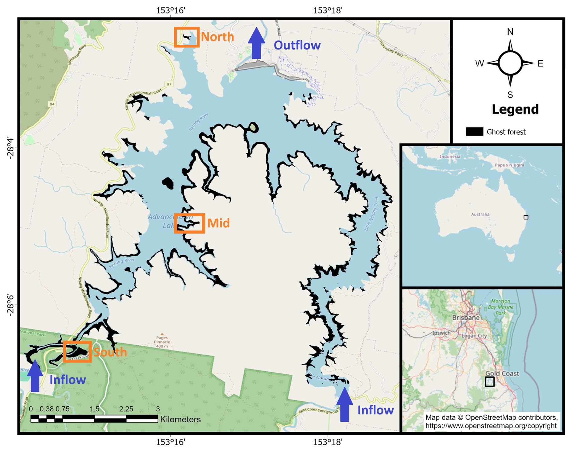
Figure 1 Map of Hinze Dam, showing the extent of the ghost forest (black) covering approximately 20 % of the reservoir surface area. The three study sites (North, Mid, and South) are marked in orange (OpenStreetMap).

2.2 Field campaigns

Two field campaigns were conducted in the winter (mid-August) and early summer (late November) of 2023 to capture seasonal variability in temperature and water level. All sampling was conducted from boats to minimize benthic disturbances within each plot. The three plots were located to the South, Mid and North of the reservoir western arm, which accounts for an inflow depositional gradient from South to North (Fig. 1). In the South, the Nerang River stream feeds the reservoir and deposits sediment and organic material. Ghost forest trees were sampled in belt transects perpendicular to the shoreline (Fig. 2a–c), which allowed us to measure trees along a water depth gradient. All trees sampled were in standing water during both field campaigns (Fig. 2d). The same trees were re-sampled in both seasons, keeping the stem height above the water surface consistent between campaigns, as the water table dropped.

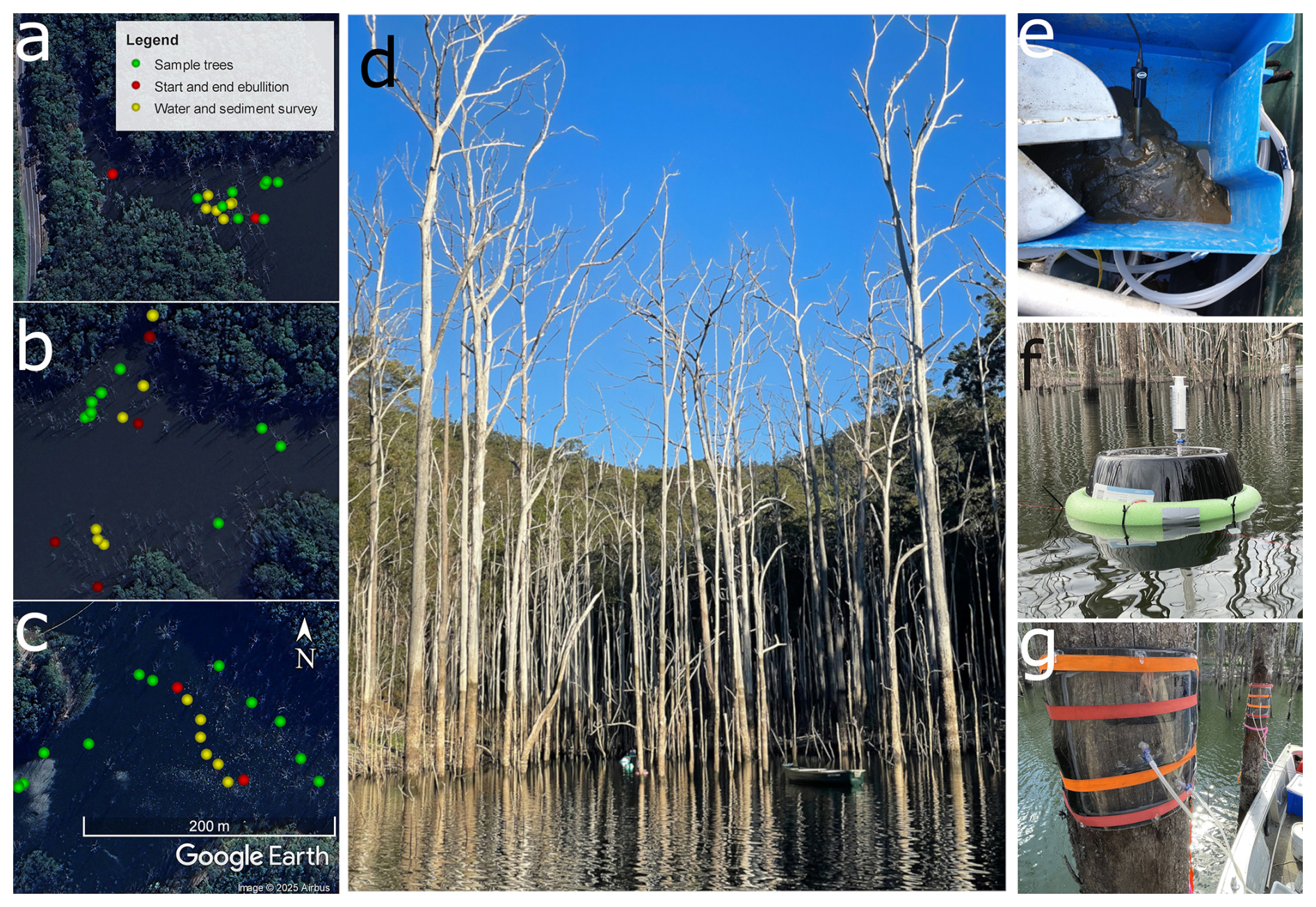
Figure 2 Layout of the three study sites in Hinze Dam during the summer campaign, showing the North (a), Mid (b), and South (c) sites. The panels show the sample trees, the start and end points of the ebullition transects, and the sediment and water survey sampling locations. Further panels show: A ghost forest embayment (d), sediment sampling (e), a floating chamber to collect ebullition (f), and a tree chamber (g).

2.3 Sediment sampling

A Van Veen grab was used to collect benthic sediments from six locations per site (Fig. 2e). The pH and redox potential of the sediments were measured in situ using a pre-calibrated multiprobe (Hach PHC101 and MTC301). During the first campaign, three soil samples were also taken at each site and analysed for total nitrogen, phosphorus and % C_org with samples oven dried at 40 °C and then homogenised before analysis. Total nitrogen was determined using a LECO TruMac CNS analyser. Soil samples for phosphorus determination were first treated with a 1:3 Nitric $/$ HCl and then run on APHA 3125 ICPMS. Carbon content samples were pre-treated with acid to remove inorganic carbon before analyses on an Elemental Analyser (EA). During the second campaign, the depth of the organic-rich layer was estimated by gently tapping a 10 cm ø PVC pipe through the softer sediments until the hard clay layer was reached, and measuring the depth change. This was replicated at three locations per site. The sediment oxygen demand (SOD) was determined by adding 10 g of freshly collected sediment (Van Veen grab) into a 250 mL borosilicate glass bottle, filling it with surface water and noting the start and stop concentrations of dissolved oxygen at 0 and 48 h using a luminescent/optical dissolved oxygen sensor (Hach, LDO101).

2.4 Aquatic CH₄ concentrations

To determine aquatic CH₄ concentrations, 150 mL water samples were collected into borosilicate bottles at six locations within each site along a water depth gradient. Surface (10 cm) and bottom water samples (30 cm above the benthic surface) were collected using a peristaltic pump, overflowing > 3 times the bottle volume before capping ensuring no headspace. The samples were initially kept on ice until later being treated with mercuric chloride (HgCl₂) at the end of the sampling day. Water temperature and dissolved oxygen levels were also measured at the same locations using a hand-held probe (Hach, LDO101). Additionally, a spatial transect collecting water samples in borosilicate bottles (as described above) at ∼ 1 km intervals along the reservoir was performed on each trip, spanning from the southern to northern plot (Winter n=16 and summer n=23 locations). The coordinates, windspeed and water depth were also noted at each sample location. All water samples in borosilicate bottles were analysed as followed: the dissolved partial pressure of pCH₄ was determined using the headspace method with a 90 mL water sample and 60 mL of ambient air added into a 150 mL syringe and shaken vigorously for 2 min (Jeffrey et al., 2019a). The headspace gas was then analysed using a CH₄ isotope cavity ringdown spectrometer (Picarro CRDS, G2201-i) and then corrected for the dilution with ambient air according to Eq. (1) (de la Paz et al., 2021):

$$\begin{array}{}\text{(1)}& {\mathrm{CH}}_{\mathrm{4},\mathrm{w}\mathrm{sample}}={\displaystyle \frac{{\mathrm{CH}}_{\mathrm{4}p}}{V_{\mathrm{w}}}}\left(K{V}_{\mathrm{w}}+{\displaystyle \frac{\mathrm{1}}{RT}}{V}_{\mathrm{V}}\right)\end{array}$$

where V_w is the volume of the water used, K is the solubility coefficient, R is the universal gas constant ($\mathrm{8.205}\times {\mathrm{10}}^{-\mathrm{5}}$ m³ atm ⁻¹ K⁻¹ mol⁻¹), T is the air temperature (K), V_V the volume of the headspace, CH_4 p is the CH₄ concentration (ppmV) measured with the SSIM CRDS.

2.5 Ebullition fluxes

To quantify ebullition at each site, ten floating chambers were established along a perpendicular transect from the shoreline within the ghost forest (n=30) (Fig. 2a–c and f). The chamber diameter was 41 and 12.5 cm height, with a total volume of 12.9 L and surface area of 0.132 m². Gas within the headspace of each chamber was collected every ∼ 24 h. Each chamber had a 30 mL syringe pre-attached to the chamber outlet, which was extracted carefully to minimize disturbance to the chamber. The 30 mL gas sample was then transferred into duplicate evacuated 12 mL exetainer vials. The gas samples were later analysed for CH₄ concentration using the CRDS and a small sample induction module (Picarro SSIM, A0314).

2.6 Tree stem and diffusive CH₄ fluxes

The ghost forest tree stem CH₄ fluxes were measured by attaching semi-rigid foam-lined airtight chambers onto the tree stems (Siegenthaler et al., 2016) (Fig. 2g). Each tree stem CH₄ flux was measured at three different heights between 10 and 220 cm above the water level to account for variability of fluxes along stem height (Pangala et al., 2013). Chambers that were attached above algae, bark or over cracks were noted (Fig. S1 in the Supplement). To prevent potential chamber leaks due to small cracks, fissures or rough bark surfaces, white pottery clay was applied to seal these areas (Jeffrey et al., 2020b). Individual gas fluxes were measured for 3 to 7 min, with longer measurements required for lower fluxing tree stem surfaces. Diffusive CH₄ fluxes were measured adjacent to ghost forest trees by placing a smaller 28 cm diameter circular floating chamber onto the water surface. The tree stem and diffusive flux chambers were connected to a portable cavity ring-down spectrometer CO₂ and CH₄ analyser (CRDS Picarro, G4301) and CO₂ and CH₄ flux rates were measured in situ. Here we only present the CH₄ data, the CO₂ results are available in the Supplement (Fig. S4–S6) and dataset (Dittmann, 2025). The CRDS precision was factory calibrated ± 0.3 ppb with a lower detection limit of 0.9 ppb. The stem circumference and flux chamber height above the water level were noted for each sample tree, along with the water depth.

2.7 Ghost forest tree stem internal gas concentrations

Ghost forest internal tree stem gas concentrations were collected from 11 trees spread across each site, similar to Carmichael and Smith (2016). Multiple 12 cm deep (13 mm internal diameter) holes were drilled horizontally into each tree stem at lower stem heights, using a cordless electric drill, with the hole immediately sealed using a sterilized rubber septum stopper. Gases were allowed to accumulate in the stem cavity for 24 h, at which time ∼ 12 mL of stem gas were removed and injected into a pre-evacuated exetainer, with the precise volume of gas sample noted. The CH₄ concentration was determined using the CRDS SSIM (as described above).

2.8 Flux calculations and upscaling

The stem and diffusive CH₄ flux (s) rate was processed using a modified gas flux R script “GasFluxes” (Fuss et al., 2020). The results of the linear regression for each flux measurement (Fig. S2) were added into the following Eq. (2) (Jeffrey et al., 2019b):

$$\begin{array}{}\text{(2)}& F=\left(s\left({\displaystyle \frac{V}{R{T}_{\mathrm{air}}A}}\right)\right)t\end{array}$$

where s is the regression slope in ppm s⁻¹ for each flux measurement, V is the chamber volume (m³) (which includes the CRDS volume, chamber and tubing volume), A is the chamber surface area (m²) and t is the conversion factor from s to d, and to µmol of CH₄. Linear regression of CH₄ fluxes of r²>0.7 were used in the calculation and linear regression with lower r² were analysed and used in the calculations when a clear increase was visible. In lower CH₄ fluxing trees, the CO₂ flux linear regression r² values were used as a proxy for assessing air-tight chamber seals, as all tree stems emitted CO₂. The ebullition CH₄ flux rates E were calculated according to Eq. (3):

$$\begin{array}{}\text{(3)}& E=\left(\left({\displaystyle \frac{{\mathrm{CH}}_{\mathrm{4}\mathrm{end}}-{\mathrm{CH}}_{\mathrm{4}\mathrm{start}}}{T_{\mathrm{d}}}}\right)\cdot \left({\displaystyle \frac{V}{R{T}_{\mathrm{air}}A}}\right)\cdot t\right)-F_w\end{array}$$

where T_d is the duration of the deployment time, CH_4 end is final headspace concentration (ppm), CH_4 start is assumed 1.9 ppm and F_w is the average diffusive CH₄ flux at each site (as determined in Eq. (1) using portable GHG analyser). As our chambers (Sect. 2.5) measured total flux (i.e. diffusive + ebullitive), the average diffusive flux was subtracted from each ebullition chamber to estimate the ebullitive flux, similar to prior studies using the same approach (Hoffmann et al., 2017; Sø et al., 2024).

To upscale the axial tree stem CH₄ fluxes to individual tree emissions, the diameter at breast height (DBH in cm) was used and trees were assumed as a cylinder with no branching. To conservatively estimate total stem gas fluxes, we only up-scaled to a height of 2.5 m above the water level (even though trees were in excess of 30 m in height). This was the highest tree stem location we measured, so we did not extrapolate beyond this point. The upscaled tree stem CH₄ fluxes were used in comparison between sites and in total reservoir upscaling. The tree was divided into three radial bands and calculated as follows (Eq. 4) similar to Jeffrey et al. (2023):

$$\begin{array}{}\text{(4)}& F_{\mathrm{t}}={\int }_{\mathrm{0}}^{\mathrm{2.5}}(c\cdot h\cdot F)\end{array}$$

where F_t is the flux per tree up to 2.5 m (µmol d⁻¹), c is the tree circumference (m), F is the in situ measured gas flux rate for that height (µmol m⁻² d⁻¹) and h is the height of each band (m). The height per band was the same as the height of the chamber plus half the distance to the next chamber, or the distance to either end of 2.5 m.

The density of ghost forest trees (trees ha⁻¹) was estimated from duplicate 100 m² plots in the Northern site and four 100 m² plots in the South and Mid sites. Tree heights were measured during May 2025 using a laser range finder (Nikon, Forestry Pro). The overall ecosystem CH₄ flux from trees for each site was calculated using Eq. (5):

$$\begin{array}{}\text{(5)}& F_{\mathrm{tol}}=x{F}_{\mathrm{t}}\cdot d\cdot c\end{array}$$

where F_tol is the total tree flux per ha (mol d⁻¹), xF_t is the average tree flux per site, d is the tree density (trees ha⁻¹) and c is the conversion factor from µmol d⁻¹ to mol d⁻¹. To upscale the diffusive and ebullition flux inside the ghost forest area, the sum of the tree basal surface areas was subtracted from the total aquatic surface area. The remaining aquatic surface area was multiplied by the average areal diffusive and ebullition CH₄ flux rates per site. (Note: tree basal areas only accounted for $\mathrm{1.6}\pm \mathrm{0.4},\mathrm{1.6}\pm \mathrm{0.5}$ and 2.5±1.0 % of the ghost forested area within South, Mid and North sites, respectively).

The total surface area of the reservoir, the ghost forested areas and the shallow zones around the edges (8 m water depth) were estimated using ArcGIS Pro (version 3.4.0), using a bathymetry map provided by Seqwater. Ebullition was assumed to only occur in all areas < 8 m in depth (Bastviken et al., 2004). For the open water areas of the reservoir (not containing trees), the diffusive CH₄ flux was estimated using spatially collected dissolved CH₄ concentrations (from the transect grab samples above) and the CH₄ flux rate numerically modelled using k estimated from windspeed (Wannikhof, 1992). We separated the reservoir surface area into three zones, the southern zone (with the inflow), the middle zone (spanning most of the open water reservoir including the eastern part) and the northern zone (which combines the far north and eastern embayment). The average flux per site for each of the three CH₄ pathways (trees, diffusive and ebullition) for each trip was used in the calculation. The sum of the three pathways represents the total zone emissions.

For better comparison we normalized the tree CH₄ flux relative to the water surface area (m²) (Amaral et al., 2025). The average tree stem CH₄ flux per site were converted to a flat surface equivalent (F_surface), tree heights were upscaled to 2.5 m and only here we also upscaled to 10 m to compare to a less conservative approach. Equation (6):

$$\begin{array}{}\text{(6)}& F_{\mathrm{surface}}=\left({\displaystyle \frac{d}{\mathrm{100}}}\right)\cdot (c\cdot h)\cdot x{F}_{\mathrm{t}}\end{array}$$

2.9 Statistical analyses

All reported errors represent standard errors of the mean. All analyses were undertaken using R (4.3.2), figures and graphs were modified using Gimp (v. 2.10.36). The Shapiro-Wilk normality test and Q-Q visualisation were used to test for normality. For normally distributed data, t-tests were applied to compared differences between groups. Otherwise, Wilcoxon rank-sum tests were used when data did not conform to normality. Differences between stem height measurements and between fluxes from the three plots were tested using Kruskal-Wallis One Way Analysis of Variance on Ranks, followed by the Dunn post hoc test for pairwise comparisons. Relationships between water depth and aquatic gas concentrations were assessed using linear models, where regression lines were fitted to log-transformed water depth.

3 Results

3.1 Site conditions

Reservoir water capacity declined during the two campaigns from 86 % in winter to 80 % in summer, resulting in a water level drop of ∼ 1.5 m (Fig. 3). This was among the lowest levels since the dam wall was raised in 2011. Average water temperatures increased from 17.2±0.1 °C in winter to 24.6±0.7 °C during summer. Water temperature was similar between the top and bottom waters inside the ghost forest areas indicating no thermal stratification. The average maximum and minimum air temperature (including 14 d prior and after the fieldwork campaign) increased from 23.9 and 5.4 °C in winter, to 29.2 and 16.0 °C in summer. During the winter campaign, the reservoir received 1.5 mm of rain, while during the summer campaign 29 mm of precipitation occurred on the first two days and 4 mm over the rest of the week.

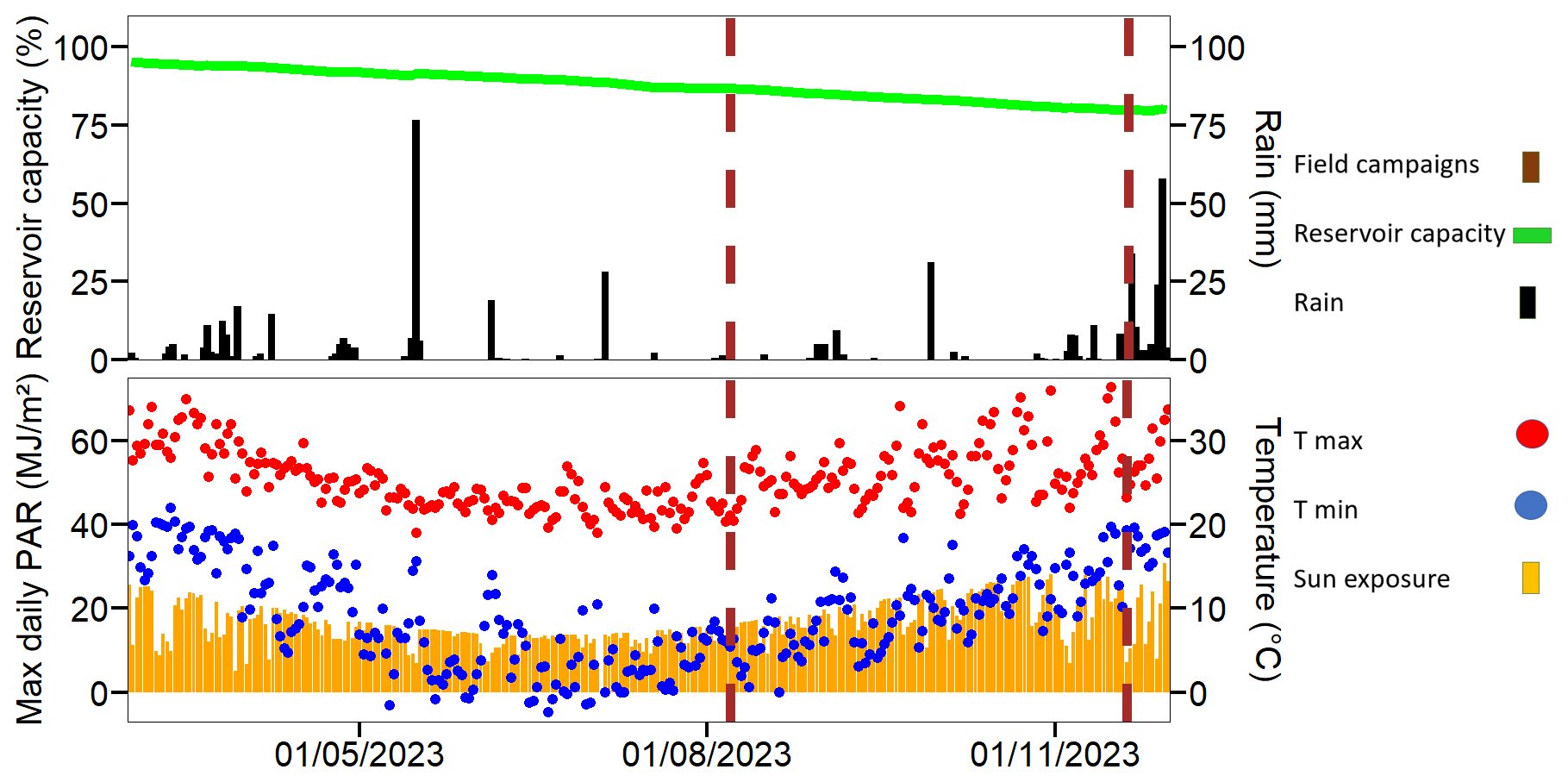
Figure 3 Climate and water level in Hinze Dam before and after sampling campaigns. Sun exposure (orange bars in MJ m⁻²) and rainfall (black bars in mm) were measured at the Hinze Dam weather station (ID 40847), while minimum (blue dots) and maximum (red dots) air temperature data (°C) were sourced from the Canungra weather station (ID 140008). Reservoir capacity (%) data were obtained from Seqwater. The timing of the two sampling campaigns is marked by red triangles.

3.2 Water physicochemistry

Dissolved oxygen (DO%) in the water column of the reservoir was lower overall during winter than in summer (Table 1). The biggest change was observed at the southern site, where bottom DO increased from 60 % to 90 % saturation between the two campaigns. The DO concentrations were 4 %, 3 % and 11 % lower at the bottom of the water column compared to surface, in the North, Mid and South sites, respectively. During the summer campaign, the difference was 11 %, 21 % and 27 % in the North, Mid and South sites, respectively. Surface water pH increased between campaigns, from 7.3 to 7.6, 7.3 to 7.9 and 7.2 to 8.3 for the North, Mid and South sites, respectively.

Table 1 Water physicochemical parameters at Hinze Dam for each of the three study sites (North, Mid, and South) for both surface and bottom water layers, during winter (South and North n=7, Mid n=6) and summer (n=6). All averages are shown with ± standard errors (SE).

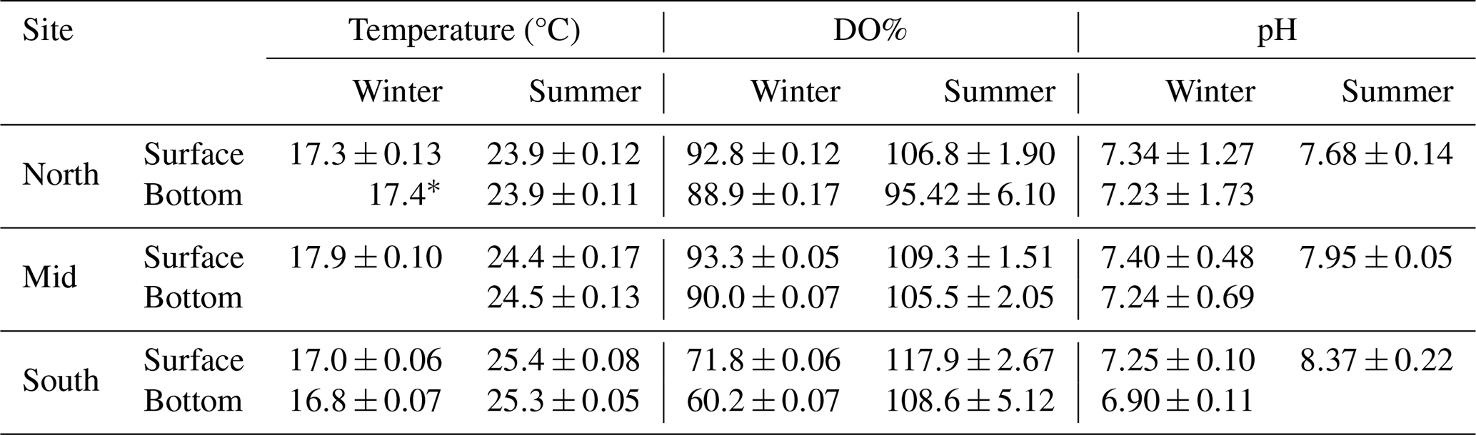
^* Only one measurement.

3.3 Benthic sediment parameters

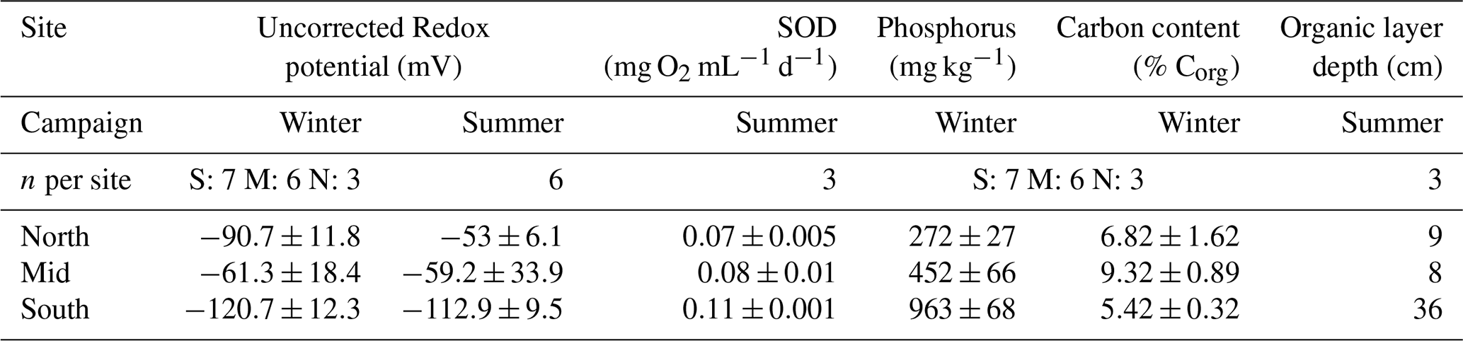
Benthic sediment organic carbon varied between sites, it was lowest at the South site (5.42 %) and highest at the Mid site (9.32 %) (Table 2). Phosphorus concentrations were the highest at the South site (963.3 mg kg⁻¹), more than double the other sites. The average uncorrected redox potential at the southern site ranged from $-\mathrm{120}\pm \mathrm{12}$ to $-\mathrm{113}\pm \mathrm{10}$ mV during the two campaigns, respectively. For the North site the average uncorrected redox potential shifted from $-\mathrm{90}\pm \mathrm{12}$ to $-\mathrm{53}\pm \mathrm{6}$ mV during summer. The Mid site had a larger variance in its uncorrected redox values during both campaigns, ranging from −121 to −85 mV on one shore to −17 to −1 mV on the opposite shore, inside the embayment. Similarly, during summer the redox potential ranged from −132 to −123 mV on one side to −62 and 53 mV on the other side of the bay. The sediments in the South site had the highest average sediment oxygen demand (SOD) with 0.11±0.001 mg O₂ mL⁻¹ d⁻¹ followed by the Mid site 0.08±0.017 mg O₂ mL⁻¹ d⁻¹ and the North site 0.07±0.009 mg O₂ mL⁻¹ d⁻¹.

Table 2 Benthic sediment characteristics at Hinze Dam at the North, Mid, and South study site locations. All averages are shown with ± SE.

3.4 Tree density, size and water surface area

Measured tree DBH ranged from 17.0 to 37.5 cm, 19.7 to 60.0 cm and 18.0 to 41.8 cm for the North, Mid and Southern site, respectively. The average tree DBH per site was 30.2±3.6 cm, 28.7±3.5 and 23.5±2.5 cm for the North, Mid and Southern site, respectively. The ghost forest tree density was 2200, 1350 and 1975 trees ha⁻¹ for the North, Mid and South sites, respectively. The tree basal areas covered between 1.5 % and 2.5 % of the water surfaces in the ghost forest areas. Tree height ranged from 10.0 to 28.8 m above the water surface and averaged 22.0±2.7 m.

3.5 Aquatic CH₄ concentrations

Dissolved CH₄ concentrations in the surface water declined at our sample locations as the water depth increased during both winter (R²=0.28, p<0.005) and summer (R²=0.43, p<0.001) (Fig. 4). Aquatic CH₄ concentrations were highest during the summer campaign.

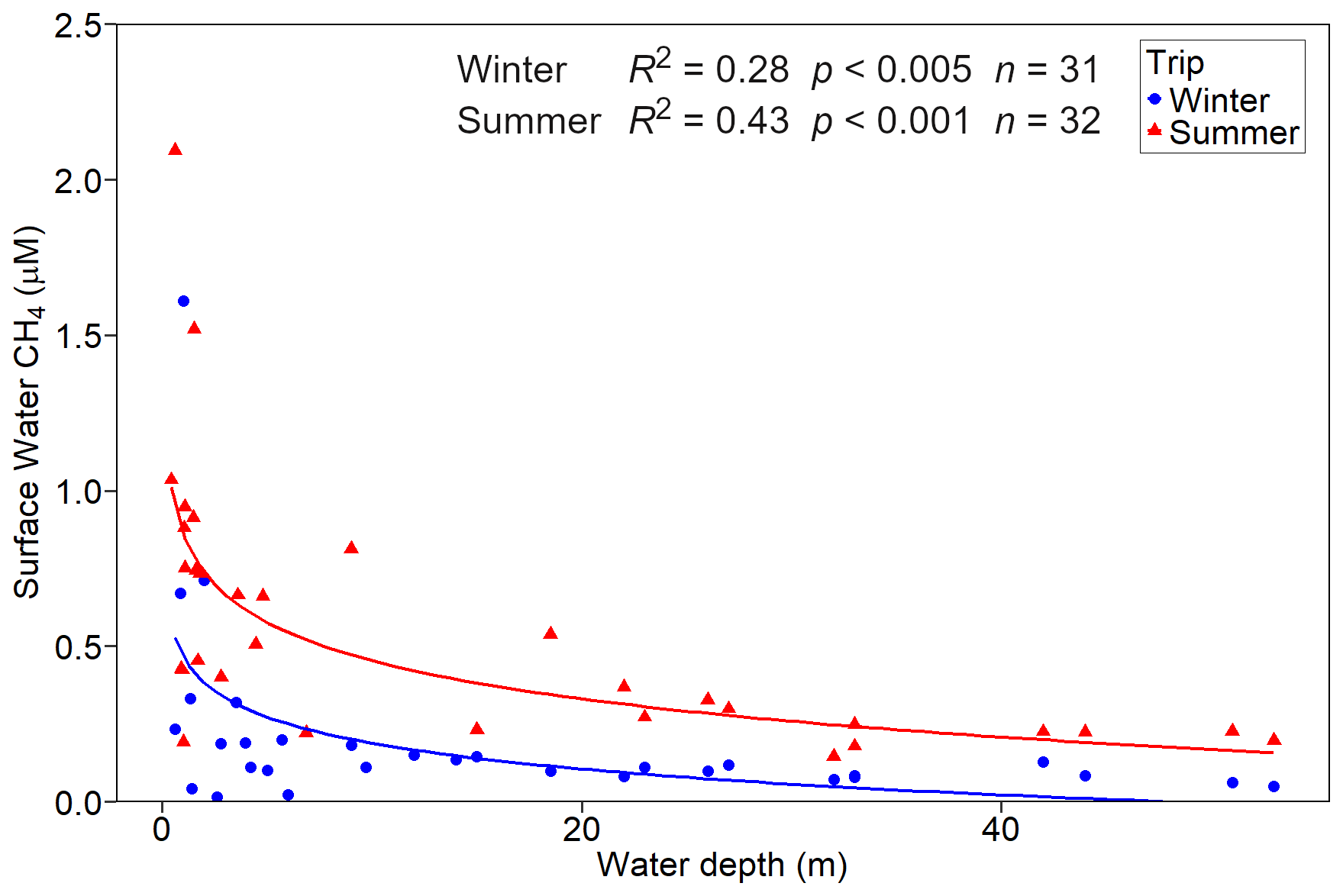
Figure 4 Surface water concentrations of dissolved CH₄ in Hinze Dam during the winter and summer campaigns. Data include samples from the three study sites and a south-to-north transect. Trend lines for significant relationships are shown.

3.6 Ebullition

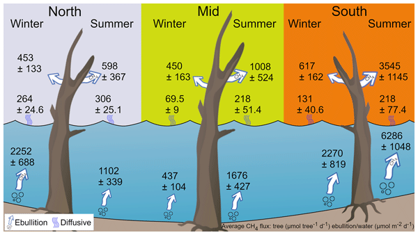
There was considerable spatial and temporal heterogeneity in the ebullition CH₄ fluxes between and within sites. In winter, the average ebullition fluxes were 2253±688, 437±104 and 2270±819 µmol m⁻² d⁻¹ for the North, Mid and South sites, respectively (Fig. 5, Table 3). During the summer, average ebullition CH₄ fluxes were 1103±339, 1677±427 and 6286±1048 µmol m⁻² d⁻¹ for the North, Mid and South sites, respectively. There was a significant increase in ebullition flux between the winter and summer campaigns for the Mid (p<0.05) and South site (p<0.005). The decreased ebullition flux at the North site between winter and summer was not significant. For the winter campaign, the ebullition fluxes showed significant difference between the Mid and North site (p<0.05), as well as the Mid and South site (p<0.05). During the summer campaign we found significant differences in the ebullition fluxes between the South and North site (p<0.005), as well as South and Mid site (p<0.001).

3.7 Diffusive CH₄ flux

Diffusive CH₄ flux rates differed between the three sites within the reservoir. During winter, the highest average diffusive CH₄ fluxes were measured at the North site (264±25 µmol m⁻² d⁻¹), followed by the South site (131±41 µmol m⁻² d⁻¹) and lowest at the Mid (69.5±7.0 µmol m⁻² d⁻¹) site (Fig. 6, Table 3). The North site showed significantly higher fluxes compared to the Mid site (p<0.001) and to the South site (p<0.005). During summer, the North had the highest average diffusive flux (306±25 µmol m⁻² d⁻¹) and Mid and South sites had similar fluxes (218±51 and 218±77 µmol m⁻² d⁻¹). Significant differences were only observed between the North and South site (p<0.01). Only the Mid site showed a significant increase in diffusive CH₄ fluxes between campaigns (p<0.001).

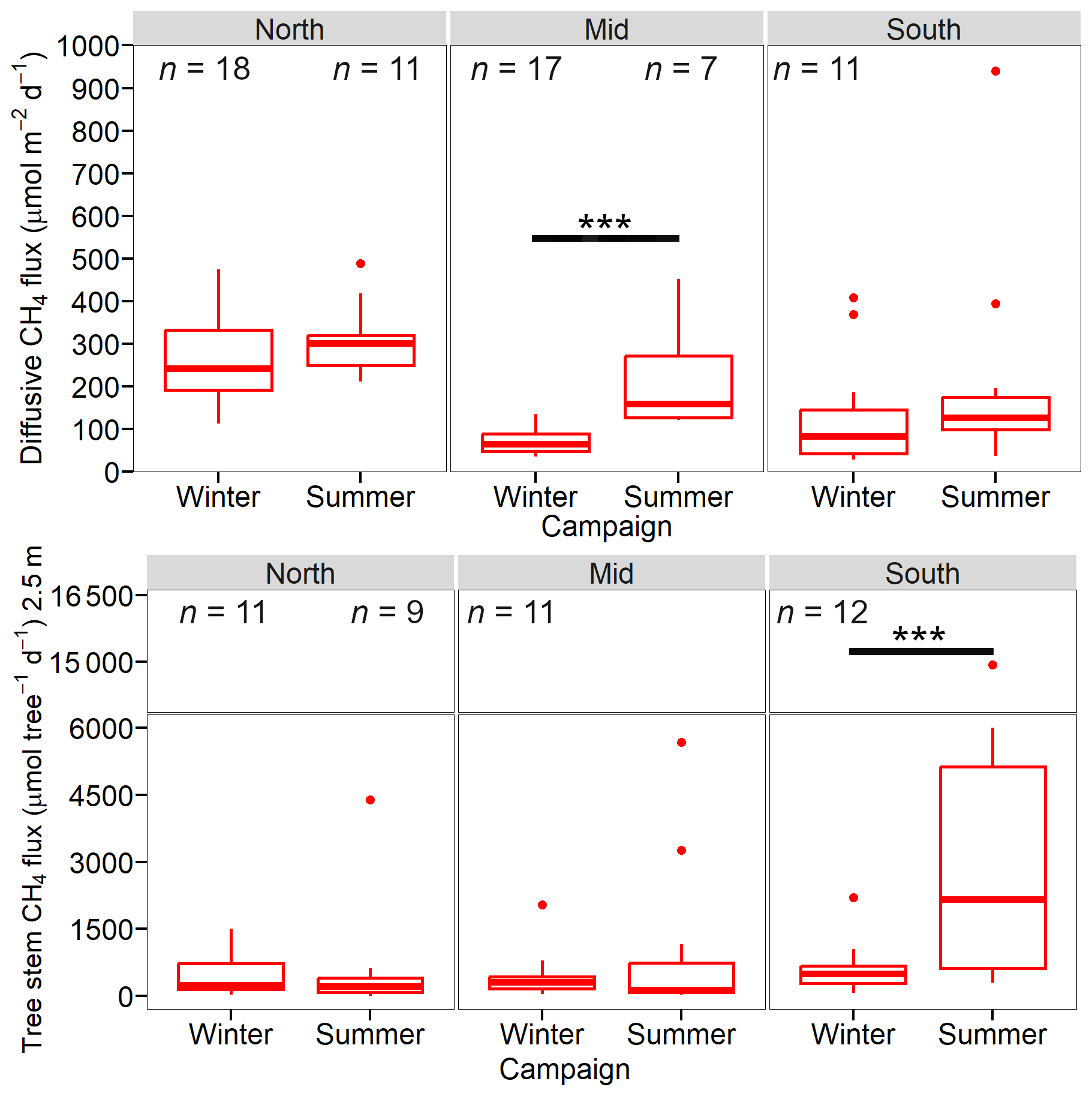
Figure 5 Diffusive CH₄ flux (top) and tree stem CH₄ fluxes (µmol per tree d⁻¹) (bottom) Tree stem fluxes were scaled to 2.5 m stem height. Significant differences are shown with the solid horizontal line.

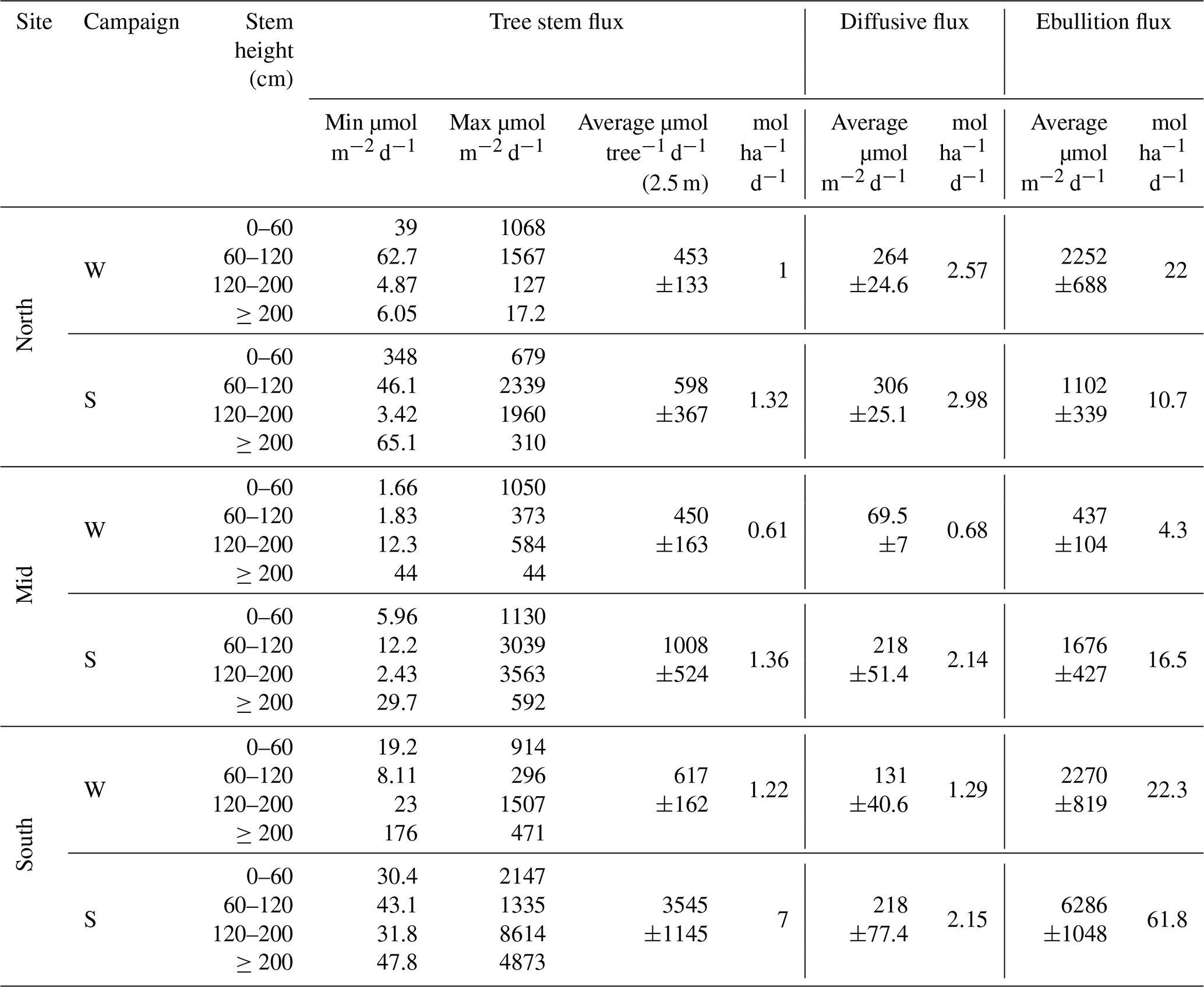
Table 3 Summary of CH₄ fluxes from ghost forest tree stems (n= winter: North: 31 Mid: 32 South: 35, summer: North: 23 Mid: 31 South: 36), diffusive (n= winter: North: 18 Mid: 17 South: 11, summer: North: 11 Mid: 7 South: 11), and ebullition pathways (n= North: 10, Mid: 9, and South: 10) during the winter (W) and summer (S) campaigns. For tree stems, the range of single measurements by stem height are included, along with the average flux and total flux per ha. For the diffusive and ebullition flux, the average and total flux per ha are reported. All averages are shown with ±SE.

3.8 Ghost forest tree stem CH₄ fluxes

All trees at all stem heights (total n=192) emitted CH₄ during both campaigns. There was a high variability in the amount of CH₄ emitted per tree at all three sites. The CH₄ stem flux measurements ranged from 1.66 to 1584 µmol m⁻² d⁻¹ and 2.43 to 8614 µmol m⁻² d⁻¹ for the winter and summer campaigns, respectively (Fig. 6, Table 3).

Average stem CH₄ fluxes per tree (upscaled to 2.5 m) were 510±90 and 1770±508 µmol per tree d⁻¹ for the winter and summer campaign, respectively. The tree CH₄ fluxes ranged from 26.8 to 2196 µmol per tree d⁻¹ during the winter campaign and from 5.34 to 14,944 µmol per tree d⁻¹ in summer.

Average tree stem CH₄ fluxes were the highest in the South site during both campaigns (Fig. 4), winter 617±162 and summer 3545±1145 µmol per tree d⁻¹ (Table 3), but only significantly different during the summer campaign (Mid-South p<0.01 and North-South p<0.005). The second highest tree fluxes were from the North site (453±133 µmol per tree d⁻¹) during the winter and the Mid site (1008±524 µmol per tree d⁻¹) during summer. Average tree stem CH₄ fluxes increased during the summer campaign, but were only significantly higher at the South site (p<0.005).

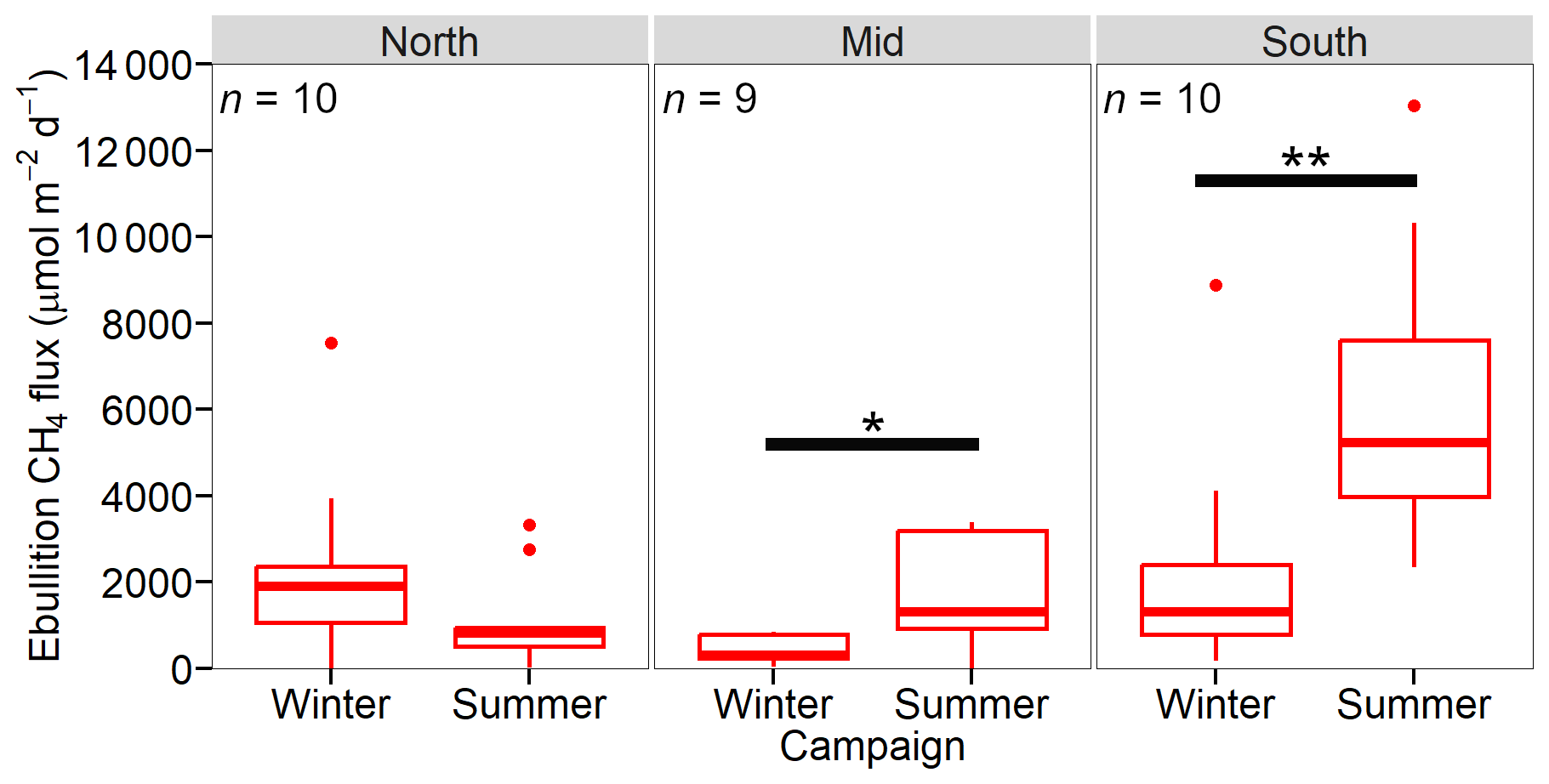
Figure 6 Average ebullition CH₄ fluxes (µmol m⁻² d⁻¹) with SE from Hinze Dam, presented for the three sites (North, Mid, and South) during both winter and summer campaigns. Significant differences are indicated with the solid black bar.

3.9 Flux versus stem height

In winter, the ghost forest stem CH₄ fluxes decreased with stem height. The average flux rates were 318±55.8, 251±57.0 and 153±54 µmol m⁻² d⁻¹ for the lower, middle and upper measurements (Fig. 7), with the lower and upper stem height fluxes being significantly different (p<0.005). One tree at the South site showed the highest flux of the campaign (1507 µmol m⁻² d⁻¹), however, the flux chamber was located over a stem fissure.

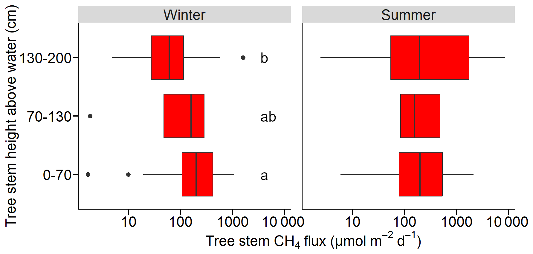
Figure 7 Tree stem CH₄ (in µmol m⁻² d⁻¹) fluxes measured at three heights (cm) above water level at Hinze Dam (n= bottom to top: winter: 31, 32 and 31, summer: 22, 27 and 29). Data includes all three study sites during both winter and summer campaigns. Letters indicate significant differences. Note: log scale for x-axis.

In summer, no significant differences between stem heights were found (Fig. 7), however the highest average CH₄ flux observed was at the uppermost measurement (1224±409 µmol m⁻² d⁻¹), especially at the South site. The internal tree stem gas samples (n=14) contained an average CH₄ concentration of 51 086±10 126 ppm (or 5.1 % saturation), being four orders of magnitude higher than the atmosphere.

3.10 Upscaling CH₄ emission pathways within the total reservoir

The surface water CH₄ concentrations decreased from south to north, during both campaigns (Fig. 8). Up scaling CH₄ fluxes to the whole reservoir showed that total CH₄ emissions tripled between the winter and summer campaigns, from 1418 to 4604 mol d⁻¹ (Table 4). Tree stem CH₄ emissions tripled between the two campaigns, from 207 to 628 mol d⁻¹ and contributed 14 % and 15 % in winter and summer emissions respectively. Overall, ebullition was the dominant CH₄ emission source (67 % in winter and 58 % in summer), while diffusive fluxes from the deeper open water contributed only 2 % and 14 % for winter and summer, with diffusive fluxes of the shallow ghost forested areas contributed 16 % and 14 % respectively.

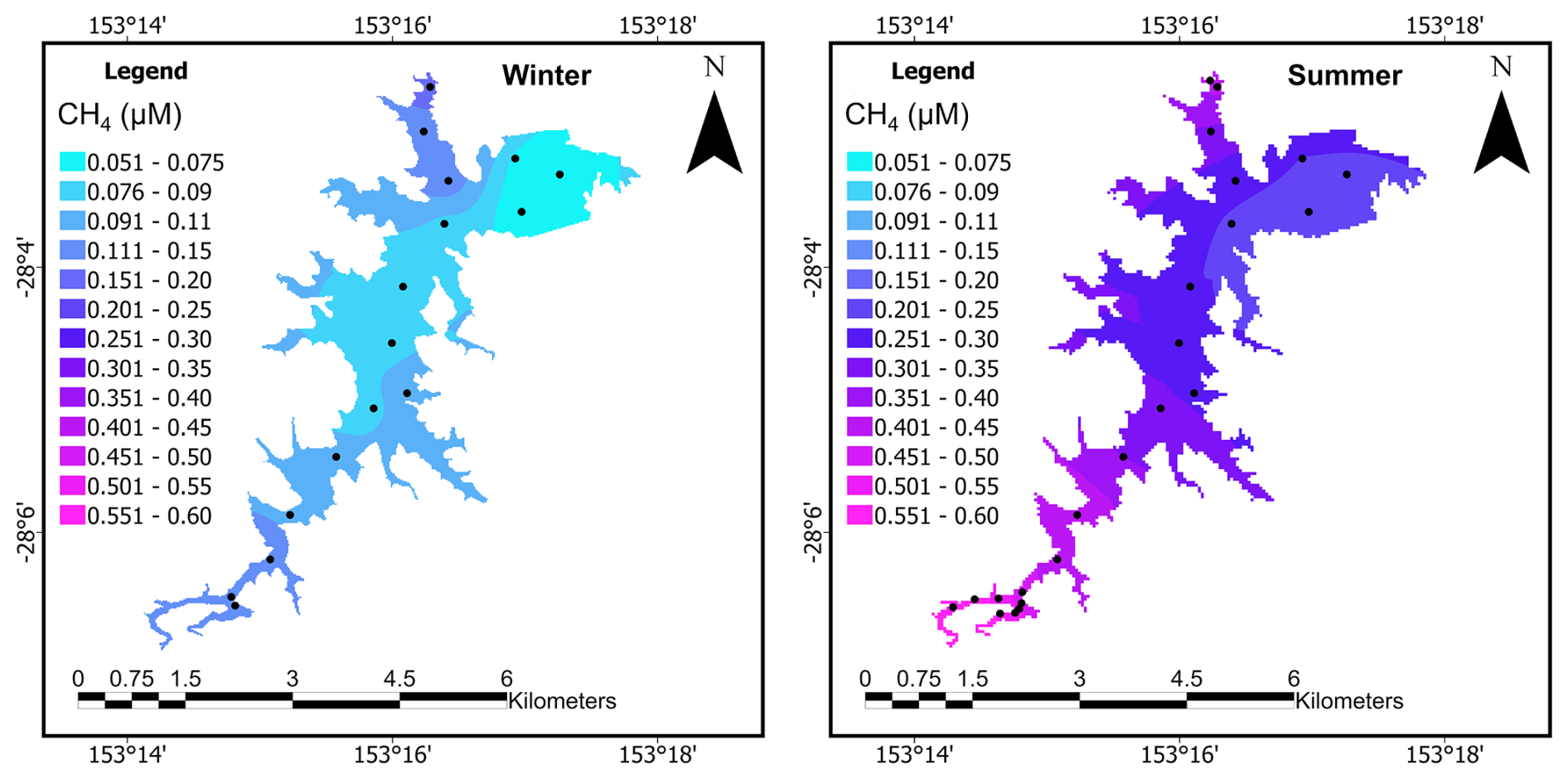
Figure 8 Surface water CH₄ (µM) concentrations in the western part of Hinze Dam, Australia (Winter n=16, summer n=23). Samples were taken along a transect from south to north in 1 km intervals (black dots), during the winter (left) and summer (right) campaigns.

Table 4 Upscaled CH₄ flux estimates for the total area of Hinze Dam, incorporating all three emission pathways.

At the flux per water surface area within the ghost forest, tree fluxes were between 56.4 and 428 µmol m⁻² surface d⁻¹, ebullition between 437 and 6286 µmol m⁻² surface d⁻¹ and diffusive flux between 69.5 and 306 µmol m⁻² surface d⁻¹. If tree stem emissions were upscaled to 10 m of stem height this increased their relative contribution at a per water surface area to between 225 and 1711 µmol m⁻² surface d⁻¹.

4 Discussion

4.1 Drivers of ghost forest tree stem CH₄ fluxes

All trees emitted CH₄ during both campaigns and from all three measured stem heights, addressing research question one. We observed high variation between the fluxes of the different trees undergoing different stages of decomposition, and due to the influence of the stem fissures and bark remnants (Jeffrey et al., 2020b). Cracks result from the decomposition and drying of the dead trees (Oltean et al., 2007). All sampled trees died at around the same time in 2011 as the water levels rose due to the raising of the dam wall. Due to their state of decomposition, we could not identify the tree species, but different species can have different decomposition rates (Freschet et al., 2012; Kahl et al., 2017). Many of large trees were likely Eucalyptus sp. based on the species in the adjacent areas located above the dam maximum water level. Eucalyptus sp. are classified as hardwoods (FAO, 2002) and therefore are somewhat more resistant to decomposition. Previous studies have found high variance in tree CH₄ fluxes even of the same species, in living (Jeffrey et al., 2023) and dead trees (Warner et al., 2017; Kipping et al., 2022). Decomposition stage is known to influence tree stem CH₄ fluxes, with recently dead trees exhibiting both elevated internal CH₄ concentrations (Covey et al., 2016) and higher CH₄ fluxes (Sakabe et al., 2025). In this study, all trees died simultaneously following reservoir inundation, meaning decomposition stage is unlikely to introduce meaningful variability among individual flux measurements. However, this dynamic may be relevant in other reservoirs where water levels rise gradually, producing ghost forests of mixed decomposition stages.

During the winter campaign, CH₄ fluxes declined with stem height, consistent with gas diffusion observations from living wetland trees, which are ecosystems featuring a clear soil CH₄ source (Jeffrey et al., 2023; Jeffrey et al., 2020a; Pangala et al., 2017; Sjogersten et al., 2020). Previous studies focused on dead tree axial trends, found that CH₄ also decreased in stem concentration, and with increasing stem height (Carmichael and Smith, 2016; Carmichael et al., 2018; Jeffrey et al., 2020b). δ¹³C–CH₄ measurements in dead trees suggest that CH₄ may be oxidized while moving upwards within tree stems, suggesting a soil source (Martinez et al., 2022). This soil source of CH₄ is further supported by research that showed wood samples produced little CH₄ during anaerobic incubations (Martinez et al., 2022).

In our study, the dead trees were in several metres of standing freshwater, featuring low-oxgyen and high SOD soil conditions. It is therefore possible that the majority of CH₄ originates from the sediments (with the trees acting as passive gas conduits) and diffuses outwards with increasing stem height. Nevertheless, due to the different decomposition states, we cannot rule out that internal microbial production of CH₄ may contribute to some of the observed CH₄ flux. The opposite trend was detected during summer, with the highest CH₄ fluxes occurring at the highest stem height. The water level had dropped ∼ 1.5 m between the two campaigns, thus potentially changing the preferential pathway of CH₄ emissions higher up the tree stems. We acknowledge that further factors, like wood water content or changing internal CH₄ production and oxidation likely also played a role. These factors complicate our system and lead us to the conclusion, that our summer results do not necessarily point to a wood source.

In living trees, it has recently been shown that CH₄ (gas phase) can travel rapidly through the bark of some wetland species, separate to the transport within the transpiration stream (liquid phase) (Jeffrey et al., 2024). Because dead trees no longer have bark and lack an active transpiration stream, this suggests that diffusion through cracks and open spaces through the dead wood may have been a more important pathway for CH₄ egress (gas phase) to be released from the reservoir sediments. However, the wood below the water line was saturated and thus reduced CH₄ diffusion rates (dissolved phase), being several orders of magnitude slower than gas. This may have led to a lag time between CH₄ production changes within the soil, and stem CH₄ gas emissions above the waterline. Further research is required to confirm both the CH₄ source(s), the transport rates and preferential pathway(s) for ghost forests.

We found no correlation between surface water depth and tree stem CH₄ flux (Fig. S3). This was similar to riparian living tree studies in the Amazon (Gauci et al., 2022) and Australian wetland forests (Jeffrey et al., 2023) which found that as the below-ground water table rose, it promoted anaerobic conditions in the soil, leading to increased CH₄ production and, consequently, higher tree fluxes. However, once surface inundation occurred, further increases in surface water depth did not significantly alter soil conditions, and therefore tree CH₄ fluxes remained similar. For the flooded ghost forest, as stem CH₄ fluxes were decoupled from variation in surface water depth, this likely reflected the dominance of soil CH₄ production, stem wood properties and decomposition state, over hydrological controls.

4.2 Seasonal variability of diffusive and ebullition fluxes

Overall, there were three-fold higher CH₄ fluxes observed during the summer campaign, along with elevated dissolved CH₄ concentrations and ∼ 7 °C increase in surface water temperature, particularly in the south site. This temperature change likely increased microbial metabolism, including methanogenesis and, therefore resulted in higher rates of CH₄ production. This was further evidenced as ebullition rates also increased in both the Mid and South sites, during summer. Temperature has been shown to enhance CH₄ flux rates (Yvon-Durocher et al., 2014) and increased ebullition in summer across multiple lake systems (Sanches et al., 2019; Aben et al., 2017). Sediments from boreal and temperate lakes have shown that CH₄ production and release increase exponentially with rising temperature (Liikanen et al., 2002; Duc et al., 2010). Previous studies have found higher ebullition fluxes above 30 °C compared to below 20 °C (Xun et al., 2024). In contrast, other studies have found that ebullition has no significant positive correlation with water temperature (Grinham et al., 2018b), suggesting organic matter content and water level changes as more important drivers. Ebullition release can also be influenced by sudden atmospheric pressure changes and wind driven turbulence (Kellner et al., 2006; Tokida et al., 2007). Aside from seasonal variability, ebullition bubble release events are highly heterogeneous (Anthony and Anthony, 2013) and temporally variable (Linkhorst et al., 2020) making them a difficult CH₄ flux term to accurately constrain (Rosentreter et al., 2021).

The aquatic surface CH₄ concentration was lower in the deep reservoir central basin, compared to the shallower ghost forested embayments. Deeper water results in a longer residence time of CH₄ within the water column, allowing for greater oxidation of CH₄. Up to 80 % of CH₄ being produced in deep water sediments can be oxidized, while CH₄ produced in shallower zones undergoes less oxidation prior to being emitted to the atmosphere (Bastviken et al., 2008).

4.3 Spatial variability of CH₄ fluxes

Methane dynamics showed notable differences among the three investigated sites, suggesting site specific factors driving CH₄ fluxes. Although temperature is a key factor, it is not the only factor influencing CH₄ concentration and fluxes. The South site consistently showed the highest ebullition and tree stem fluxes between all three sites, confirming research question two. The South site is located at the inflow into the reservoir through the Nerang River, resulting in fresh organic matter being deposited into this section of the reservoir. Even though the organic carbon concentration in the sediment was similar between the three sites, the depth of the organic layer in the South site was ∼ 3-fold deeper (< 30 cm compared to > 10 cm), leading to greater substrate availability for methanogenesis, likely explaining the higher tree and ebullition CH₄ fluxes observed. Similar to our findings, a study at nearby Little Nerang Dam, Australia (upstream from the eastern inflow), found that the ebullition fluxes were driven by sediment organic matter content, especially at the inflow site (Grinham et al., 2018b). Other studies have reported organic matter availability influencing ebullition CH₄ fluxes (Casper et al., 2000; Sobek et al., 2012) and have shown higher ebullition at inflow sites in reservoirs (Tušer et al., 2017; Shi et al., 2025; DelSontro et al., 2011). A previous study at Hinze Dam, before the dam was raised, also found the highest fluxes in the south-west of the reservoir at the same inflow site (Sherman and Ford, 2011).

The lability of the carbon in the organic material and the microbial community in the sediments should also be considered. Studies have found that CH₄ production is closely linked to the degradability of the organic material (Praetzel et al., 2020; Grasset et al., 2018; Zhou et al., 2025; Berberich et al., 2020). Phosphorus is also an important nutrient for microbial growth. The South site sediment had the highest phosphorus concentrations, which has been linked to increased primary and higher CH₄ production (Bastviken et al., 2004). In addition, another proxy for microbial activity and organic matter lability is the sediment oxygen demand (SOD). During the summer SOD was highest at the South site, further confirming the assumption that there is more easily degradable organic material and higher microbial activity within the sediment. Our findings also show lower aquatic dissolved oxygen concentration at the bottom of the water column and the lowest dissolved oxygen concentration at the South site. Oxygen consumption and the resulting depletion in the water column is usually driven more by SOD in shallow aquatic ecosystems, than water column oxygen consumption (MacPherson et al., 2007; Caldwell and Doyle, 1994).

4.4 Comparison with other studies

This is the first study measuring CH₄ fluxes from ghost forest trees inside a reservoir. Ghost forests can originate from diverse forest types and due to different causes. Due to this heterogeneity, ghost forest tree CH₄ fluxes are still relatively unexplored. Therefore, further measurements across different environments are needed to compare with our reservoir observations and better constrain the potential range of CH₄ emissions from ghost forest tree stems. Compared to those previous ghost forest tree CH₄ studies, our average CH₄ stem fluxes were within the reported range addressing research question one. However, it should be noted that each study considered a different amount of stem height measurements (Table 5). As CH₄ fluxes can change with stem height, the height and number of heights measured can strongly influence estimated fluxes. One tree in our study emitted the highest single flux from a dead tree, almost twice that of previous maxima (Table 5), highlighting potential for extreme heterogeneity. One reason our higher CH₄ fluxes may occur is because our study was located within a subtropical region, featuring higher CH₄ production and fluxes, compared to temperate climates. Although Jeffrey et al. (2019b) studied mangroves in tropical regions, seawater-derived sulphate in mangrove ecosystems likely lowered soil CH₄ production. Sulphate and iron reducers can outcompete methanogens for H₂ or acetate when sulphate and iron are available (Roden and Wetzel, 2002). Similarly, salinity and sulphate on coastal forests can influence soil CH₄ production (Martinez and Ardón, 2021) and reduce tree CH₄ fluxes. Our study showed that the site conditions in a freshwater reservoir ghost forest were favourable for high CH₄ production.

Table 5 Comparison of average and maximum CH₄ from dead tree stems and stem debris between this study and previous studies. For Jeffrey et al. (2019) only fluxes from dead mangroves are included. The highest reported average stem CH₄ concentration per study is presented here.

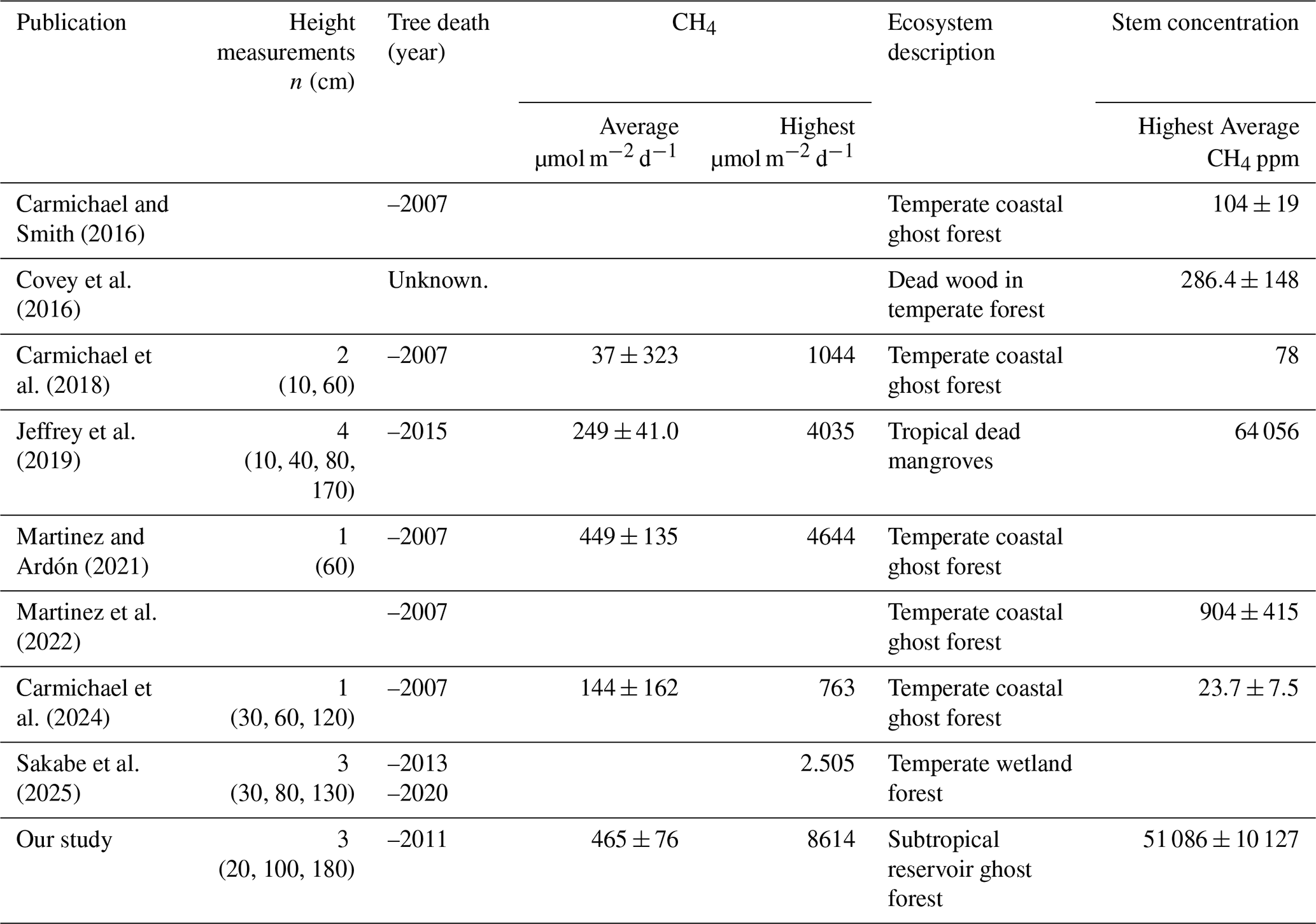
Internal stem CH₄ gas concentrations were similar to that of subtropical dead mangroves, but higher than the other studies. This may be attributed to the longer incubation period (24 h) used in our study, compared to others, which typically have incubation times under one hour. Additionally, our stem gas concentrations were collected during the summer campaign, when higher tree fluxes and potentially elevated stem gas concentrations were observed likely due to increased microbial activity. Importantly, we did not observe any uptake of CH₄ which had previously been observed in ghost forest trees (Martinez and Ardón, 2021). Previous studies measured net CH₄ uptake in 38 % and 20 % of their measurements, respectively (Carmichael et al., 2024; Carmichael et al., 2018). Carmichael et al. (2024) found sequencing based evidence for methanotroph communities inside dead trees, showing the potential oxidation capacity, whilst our results suggest that net CH₄ emissions exceeded any CH₄ oxidation.

4.5 Importance of ghost forest tree stem CH₄ emissions

Our study reveals that reservoir ghost forest trees can emit a substantial amount of CH₄ to the atmosphere. Our subtropical ebullition rates were the largest contributor to overall reservoir CH₄ fluxes at 58 % and 67 %. Studies have found herbaceous (non-woody) plant-mediated diffusion can dominate shallow aquatic CH₄ fluxes, with ebullition only playing a minor role (Jeffrey et al., 2019a; Whiting and Chanton, 1992; Chanton et al., 1992; Bastviken et al., 2023). However, in small and shallower lakes in Europe, and ponds in Australia, ebullition was determined to be the primary CH₄ source to the atmosphere (Schmiedeskamp et al., 2021; Grinham et al., 2018a). Indeed, ebullitive fluxes have been estimated to account for 80 % of the total reservoir flux globally (Johnson et al., 2021), especially within (sub)tropical regions (Harrison et al., 2021). Despite our deployment strategy (and daily sampling) of ∼ 60 ebullition chambers, spanning three sites and various water depth gradients – our sampling approach is still seasonally limited, and it therefore remains challenging to draw a definitive conclusion. Greater temporal and spatial sampling approaches would reduce these uncertainties and better constrain this CH₄ flux term. Degassing downstream of the dam wall has been found to emit significant amount of CH₄ (Harrison et al., 2021). This is particularly important in hydropower dams. However, Hinze Dam is a drinking water reservoir and water outflow of surface water is restricted (none during 2023) resulting in minimal degassing. Although we could not quantify that pathway, we argue that it is not a significant contributor in our system.

Ghost forest tree stem CH₄ contributions of 15 % and 14 % during winter and summer, respectively, suggest a persistent, and substantial CH₄ source, addressing research question three. We acknowledge that extrapolating reservoir-wide emissions from only three sites should be considered with caution, particularly given the absence of data from the eastern part of the reservoir. Also, our approach to collect ebullition likely underestimates this term, as CH₄ saturation within the headspace of the floating chambers may limit the continued diffusion of the gas. However, tree stem upscaling was done conservatively to only 2.5 m of stem height, therefore ghost forest tree CH₄ flux contribution may well be underestimated. Future studies should therefore consider ghost forest tree stem emissions, when ghost forests are present, to improve the accuracy of reservoir greenhouse gas budgets. Furthermore, because we used the Mid site – which exhibited lower emissions compared to the other sites – to scale up for large areas of the reservoir, our approach likely results in a conservative estimate of ebullition and total emission. Previous estimation of CH₄ emissions of wood decay in a reservoir represented 26 %–45 % integrated over 100-year time scale (Abril et al., 2013). Here we measured the CH₄ flux emitted by the trees, including CH₄ originating from the sediments. Based on our findings, emissions based on total carbon biomass are underestimating overall emissions, and it is crucial to measure the actual CH₄ flux from the trees. Although this pathway will eventually cease as trees decompose and disappear, the high moisture content of the timber slows decay and likely prolongs emissions.

Comparing the three CH₄ pathways at a per water surface area, ghost forest trees (upscaled to 2.5 m) contribute up to 428 µmol m⁻² water-surface d⁻¹. This is greater than the average diffusive flux (306 µmol m⁻² surface d⁻¹), but ebullition (6286 µmol m⁻² surface d⁻¹) is still the main contributor on water-surface areal basis. Comparing the fluxes on a per surface area has its limits, due to the three dimensions of trees, but it can help show the differences and directly compare between the fluxes. When upscaled to 10 m stem height (or about half way to the canopy), the contribution of ghost forest tree fluxes would increase to 1711 µmol m⁻² surface d⁻¹, demonstrating the sensitivity of upscaling total flux estimates to other stem heights.

Pre-impoundment vegetation clearing is a recognized management strategy and can been implemented prior to dam construction. This harvesting of timber would prevent emissions of CH₄ from ghost forest trees. Dams are sometimes constructed in rugged, hilly terrain to maximize storage capacity, making large-scale timber removal logistically difficult and cost-prohibitive. Trees were cleared during the initial construction of the Hinze Dam, but once the reservoir was filled and the dam level increased, it was difficult to reach the trees at the then edges of the reservoir.

5 Conclusions

This study advances our understanding of seasonal changes influencing reservoir CH₄ fluxes, and provide the first estimates of ghost forest tree stem CH₄ emissions and their contribution to the total reservoir CH₄ budget. Our findings reveal high system variability and potential CH₄ local hotspots inside reservoirs at inflow zones, where higher organic matter availability and temperature-driven microbial activity likely enhance CH₄ production (Fig. 9). These results emphasize the contribution of ghost forest trees fluxes in reservoir greenhouse gas budgets and can help guide future management decisions around ghost forest creation.

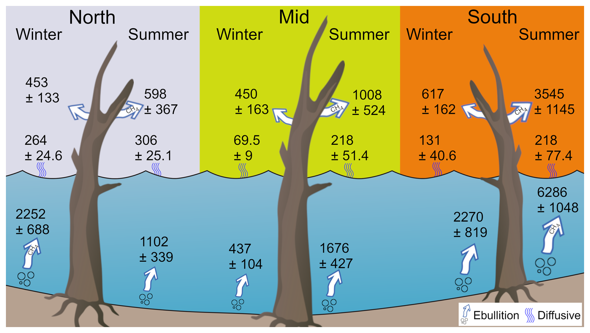
Figure 9 Conceptual figure summarising the three pathways for CH₄ (tree in µmol tree⁻¹ d⁻¹ and ebullition/diffusive in µmol m⁻² d⁻¹ and ± is SE) between the three sites and for the winter and summer campaigns. Graphics: Tracey Saxby, Integration and Application Network (https://ian.umces.edu/media-library/, last access: 26 March 2026).

We demonstrated that ghost forest trees can play a substantial role in reservoir greenhouse gas emissions and where present, they should be accounted for in reservoir greenhouse gas budgets. We suggest that the major source of tree stem CH₄ emissions likely come from the soil, but further research incorporating microbial genetic sequencing, stable isotope tracing and wood and soil incubations would be necessary to confirm this. Additional research is required to further understand changing CH₄ hotspots on stems during the seasons.

Aside from greenhouse gas emissions, ghost forest trees also provide other important ecosystem functions. They serve as habitat for birds and fish for hunting and nesting. However, quantifying these benefits against potential greenhouse gas emissions is challenging. Future management decisions should carefully assess the costs, feasibility and benefits associated with removing the trees during reservoir construction stages.

Despite the increasing body of research on tree CH₄ fluxes, substantial knowledge gaps remain, particularly concerning ghost forest trees. These unique ecosystems are expected to become more prevalent due to climate change and other anthropogenic modifications of ecosystems, underscoring the critical importance of further investigations and baseline information.